Energy Management Strategy for a Hybrid Commercial Vehicle Considering Road Gradient

Abstract

To improve the energy efficiency of hybrid commercial vehicles under varying road gradients, this study develops a road-gradient-aware hierarchical energy management framework. An interactive multiple-model Kalman filter (IMM-KF) is employed to estimate the current road gradient by fusing information from vehicle dynamics and onboard measurements. At the vehicle level, an MPC-based strategy uses future route-gradient information extracted from a pre-reconstructed road profile, rather than predicted by the IMM-KF, to plan an energy-efficient speed trajectory and reduce vehicle energy demand. At the powertrain level, a particle swarm optimization (PSO)-calibrated adaptive equivalent consumption minimization strategy (PA-ECMS) allocates the resulting power demand between the engine and motor, with the SOC-feedback PI parameters calibrated offline. The framework is evaluated in MATLAB R2024a/Simulink using standard driving-cycle and real-road data-based simulation scenarios. The IMM-KF achieves an RMSE of 0.04461° under constant-gradient conditions and 0.47587° under variable-gradient conditions. The upper-layer MPC reduces wheel-end energy consumption by 10.98% compared with PID-based speed control, while PA-ECMS reduces the comprehensive operating cost by 15.3% relative to A-ECMS under the prescribed CHTC-LT cycle. In the integrated real-road simulation, MPC + PA-ECMS reduces fuel consumption and comprehensive operating cost by approximately 4.0% and 4.7%, respectively, compared with PID + A-ECMS. These results demonstrate the effectiveness of coordinating road-gradient estimation, economic speed planning, and hybrid power allocation within the proposed hierarchical framework.

1. Introduction

Hybrid power technology, as an efficient energy management solution, has become the key to promoting the green transformation of commercial vehicles. Through the coordinated operation of engines and motors, hybrid commercial vehicles can achieve optimized energy management under different working conditions, thereby significantly reducing fuel consumption and carbon emissions, and providing strong support for promoting a low-carbon economy and sustainable development.

Road information is an important factor affecting vehicle power demand and energy consumption. Accurate and fast estimation of road surface information such as road slope can reduce fuel consumption [1]. Accurate road information and slope estimation play a crucial role in vehicle control and economy [2,3,4,5,6]. Jia et al. [7] reported that, using high-precision maps and GPS signals, vehicle position can be accurately determined, enabling advanced acquisition of detailed road information, but using the vehicle high-precision map will increase the cost. Lin et al. [8] proposed a road slope and distance estimation method based on visual–LiDAR fusion, where lane lines are detected and road slope is estimated from vanishing point coordinates. Although the model can achieve accurate identification, it depends on the lane detection method, and the problem of inaccurate identification may occur in road sections without lane lines. Kalman filter algorithm [9] and its derivative algorithm [10,11,12] combined with gated recurrent neural network [13], nonlinear prediction filter [14], and recursive least squares method [15] are also commonly used to estimate road slope. These methods usually need to establish a vehicle dynamics model and estimate the slope with acceleration and speed data. However, this kind of method cannot solve the decoupling of vehicle parameters and external resistance changes, and the change in road slope also increases the complexity of estimation, which may lead to inaccurate estimation results. The predictive energy management strategy based on full-factor information proposed by Yue et al. [16] takes into account vehicle speed, slip ratio, and slope, providing an information foundation for energy management. At the same time, it also increases the difficulty of data processing. In the work of Tao et al. [17], in structuring a stratified energy management strategy, the terrain information is predicted based on multi-long short-term memory network, which improves the economy compared with the traditional method based on TD3, but the computational complexity is high and the accuracy decays rapidly with the increase in the forecast period. Chai et al. [18] proposed an adaptive equivalent fuel consumption minimization strategy considering road section information. By analyzing the boundary of the optimal equivalent factor and its sensitivity to road slope, the strategy is classified into SOC-based and estimation-based adaptation. The results show that the proposed strategy has good robustness and feasibility.

Secondly, the economic speed-planning method mainly focuses on traffic signal information, preceding vehicle information, and road slope characteristics. The strategy based on road slope information mainly reduces additional energy consumption on slopes by optimizing vehicle speed. The dynamic programming algorithm improves the energy utilization by optimizing the vehicle energy consumption and the vehicle speed trajectory [19]. Wang et al. [20] proposed a predictive cruise control algorithm for commercial vehicles. The method predicts upcoming road slopes using map information and determines the optimal economic speed via dynamic programming. On the basis of studying the economic cruising speed change mode of vehicles under ramp road conditions, Qu et al. [21] proposed the on-trend speed adjustment method of minimum equivalent energy consumption, which could effectively improve the energy efficiency utilization of vehicles. The enhanced equivalent fuel minimization strategy integrates kinetic energy management into the equivalent fuel consumption minimization framework to improve fuel efficiency [22]. The speed-planning methods based on road slope can accurately adjust the vehicle’s driving speed on the slope, avoid unreasonable acceleration or braking when driving on the slope, and improve the fuel economy. The vehicle speed management algorithm proposed by Polverino et al. [23] can provide real-time recommended speeds for drivers, and this method has good universality for vehicles.

Hybrid electric vehicle (HEV) energy management aims to improve overall energy utilization by optimally allocating power between the internal combustion engine and the electric motor. In this field, rule-based, optimization-based, and learning-based strategies have become major research directions [24]. Li et al. [25] proposed a deep-learning-based energy management strategy that incorporates terrain information, enabling accurate perception and adaptation to complex and varying road conditions. However, this approach still suffers from several limitations, such as low training efficiency and limited generalization capability. Rule-based energy management strategies rely heavily on expert knowledge and extensive engineering experience to design control logic. Optimization-based methods, including adaptive energy management approaches [26], equivalent consumption minimization strategy (ECMS) [27], and model predictive control (MPC) [28,29], determine the optimal power split between the engine and the motor through online or offline optimization frameworks. Reinforcement-learning-based energy management strategies have attracted increasing attention due to their ability to overcome the limitations of fixed rule structures and dynamically adapt to complex driving conditions, thereby reducing energy consumption and improving system efficiency. However, these methods depend strongly on high-quality driving data and require extensive training, leading to high computational and data acquisition costs [30]. In addition, deep- and reinforcement-learning-based energy management methods are often criticized for their “black-box” nature, resulting in poor interpretability. Their performance may also degrade significantly under distribution shifts or system parameter variations, which further limits their generalization ability and transfer performance in real-world applications [31].

Road and preview information have been increasingly considered in energy-efficient vehicle control. Tota et al. [32] investigated the influence of road inclination on hybrid powertrain energy management, He et al. [33] incorporated predicted road grade into MPC-based HEV energy management, and Ciravegna et al. [34] demonstrated the potential of preview-based predictive longitudinal control for energy saving. Building on these studies, the present work focuses on the hierarchical coordination of road gradient estimation, vehicle level economic speed planning, and lower-layer power allocation rather than on the novelty of the individual control algorithms. Specifically, the IMM-KF estimates the current road gradient, the upper-layer MPC performs economic speed planning using route gradient information, and the lower-layer PA-ECMS allocates the resulting power demand, with its SOC-feedback PI parameters calibrated offline by PSO.

The main contributions of this paper are as follows:

(1)

An IMM-KF-based road-gradient estimation module is established and validated under constant- and variable-gradient conditions to provide reliable gradient information for the hierarchical framework.

(2)

A spatial-domain MPC-based upper layer is formulated to perform economic speed planning using route-gradient information, thereby reducing vehicle-level energy demand.

(3)

A PA-ECMS lower layer is developed by using PSO to calibrate the SOC-feedback PI parameters of A-ECMS offline, improving engine–motor power allocation under the investigated operating conditions.

(4)

These modules are coordinated within a hierarchical framework for a plug-in hybrid commercial vehicle and evaluated progressively through gradient-estimation, upper-layer, lower-layer, and integrated simulations using standard-cycle and real-road data.

The structure of this paper is organized as follows. Section 2 provides a detailed description of the battery modeling and longitudinal vehicle dynamics modeling. In Section 3, the energy management strategy considering road gradient is introduced. Section 4 presents the measurement-based validation of the road-gradient estimator and the simulation-based evaluation of the proposed control strategies. Finally, Section 5 summarizes the main contributions and findings of this study and outlines directions for future research.

2. Model

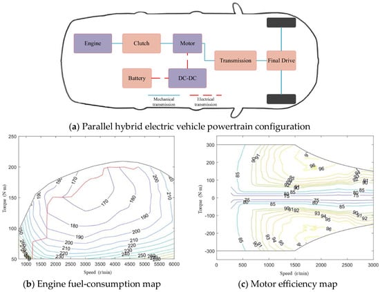
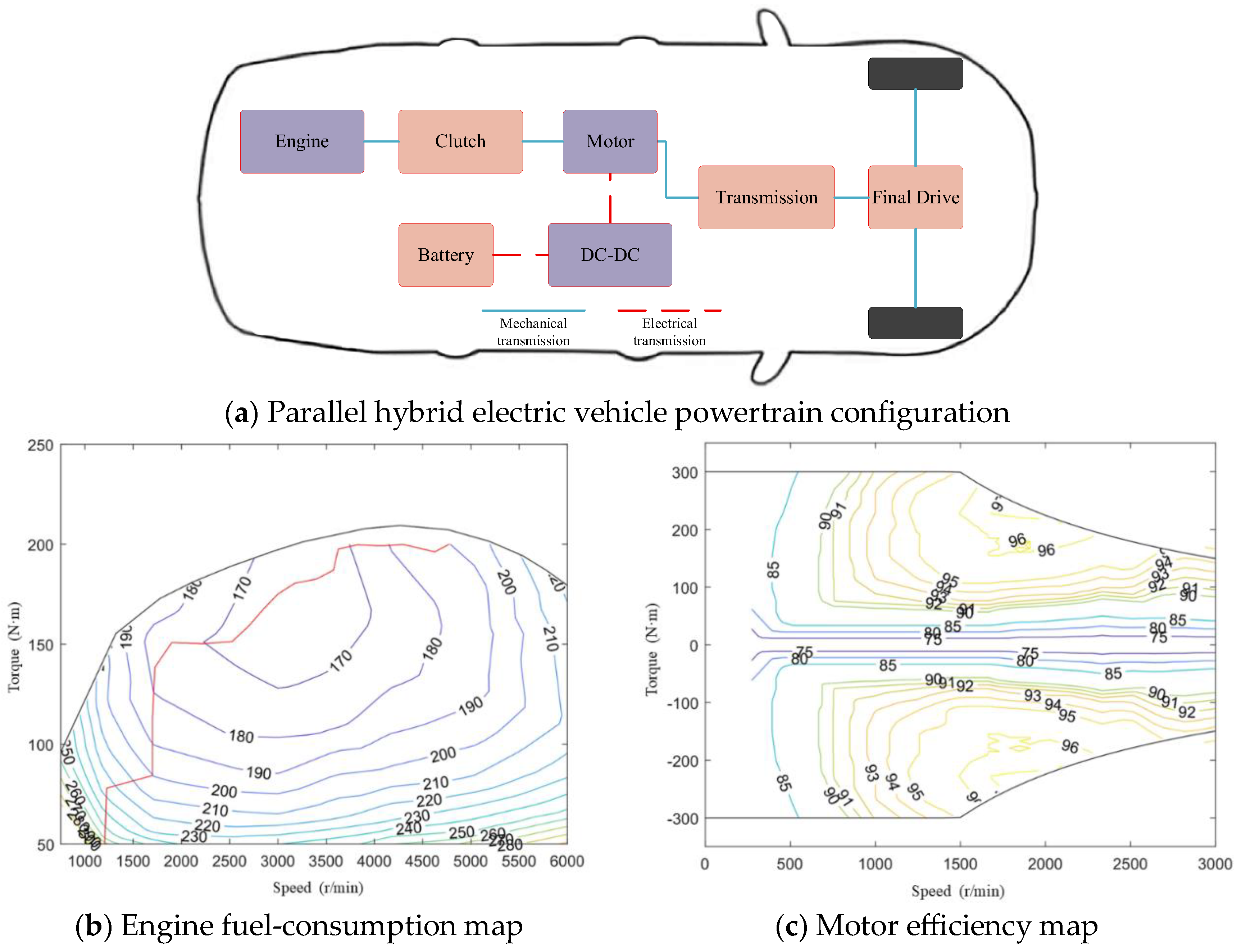
Plug-in hybrid vehicles feature dual power sources and can flexibly switch between different operating modes according to driving conditions. This study focuses on a plug-in hybrid vehicle with a parallel P2 configuration, whose powertrain consists of an internal combustion engine, an electric motor, a battery, and a transmission system. The P2 powertrain architecture and the characteristic maps used for engine and motor modeling are shown in Figure 1. The engine fuel consumption is determined by two-dimensional interpolation of the speed–torque fuel-consumption map in Figure 1b, while the motor efficiency is obtained from the speed–torque efficiency map in Figure 1c. The main performance parameters of the plug-in hybrid electric vehicle are summarized in Table 1.

Figure 1. Powertrain model and component characteristic maps. Note: In (a), background colors distinguish the powertrain components, blue solid lines indicate mechanical power transmission, and red dashed lines indicate electrical energy transmission. In (b) and (c), the colored contour lines represent different levels of engine fuel consumption and motor efficiency, respectively.

Table 1. Performance parameters of plug-in hybrid electric vehicles.

Part Name	Parameter Name/Unit	Parameter Values
Engine	Maximum power (kW)	92
	Peak torque (N·m)	350
Motor	Maximum power (kW)	60
	Peak torque (N·m)	400
Battery	Rated voltage (V)	499.2
	Battery capacity (Ah)	12
Full vehicle	Kerb weight (kg)	3600
	Gross mass (kg)	4495
	Frontal area (m2)	6.38
	Tire rolling radius (m)	0.388
Transmission system	Coefficient of air resistance	0.5
	Transmission gear ratio	5.67/2.97/1.67/1/0.76
	Final drive ratio	4.33

The engine fuel consumption is determined by two-dimensional interpolation of the engine speed–torque fuel-consumption map, while the motor efficiency is obtained by two-dimensional interpolation of the motor speed–torque efficiency map. In the energy management model, the initial battery SOC is set to 50%, and the battery SOC is constrained within [40%, 60%]. Considering the focus of this study, the transmission losses are represented using a constant mechanical transmission efficiency of 95% throughout the simulation.

The investigated plug-in hybrid vehicle is capable of both electric-only driving and cooperative operation of the engine and the electric motor, thereby supporting multiple operating modes, including pure electric mode, engine-driven mode, and hybrid driving mode. The vehicle can switch among these operating modes according to the driving conditions and battery SOC. The operating states of each component under different driving modes are summarized in Table 2.

Table 2. Operating modes of the parallel plug-in hybrid electric vehicle.

Operating Mode	Engine State	Motor State	Power Source
Engine drive mode	On	Off	Engine
Motor drive mode	Off	Motoring	Motor
Hybrid drive mode	On	Motoring	Engine and Motor
Vehicle charging mode	On	Generating	Engine
Regenerative braking mode	Off	Generating	Vehicle kinetic energy

2.1. Battery Model

An internal-resistance equivalent circuit model is adopted to characterize the battery behavior. To avoid ambiguity, the sign convention of the battery variables is defined as follows. The positive direction of battery current is defined as the discharge direction. Therefore, $I_{bat}>0$ and $P_{bat}>0$ indicate battery discharge, whereas $I_{bat}<0$ and $P_{bat}<0$ indicate battery charging.

The battery current is calculated as follows:

$$I_{bat}(k)={\displaystyle \frac{E_{bat}(k)-\sqrt{E_{bat}{(k)}^2-4R_{bat}(k)\cdot P_{bat}(k)}}{2R_{bat}(k)}}$$

(1)

where $I_{bat}$ denotes the battery current, $E_{bat}$ is the battery open-circuit voltage, $R_{bat}$ is the equivalent internal resistance, and $P_{bat}$ is the battery power. The battery terminal voltage $U_{bat}$ is related to the open-circuit voltage and battery current by $U_{bat}=E_{bat}-R_{bat}{I}_{bat}$.

Accordingly, when $I_{bat}=0$, the battery terminal voltage is equal to the open-circuit voltage, i.e., $U_{bat} = E_{bat}$. During discharge, $I_{bat}>0$, and therefore $U_{bat} < E_{bat}$, whereas during charging, $I_{bat}<0$ and $U_{bat}> E_{bat}$. The open-circuit voltage $E_{bat}$ and internal resistance $R_{bat}$ are parameterized as functions of SOC using lookup tables, with separate characteristic data for charging and discharging conditions.

The battery power is calculated as follows:

$$P_{bat}=U_{bat}{I}_{bat}$$

(2)

where $U_{bat}$ denotes the battery terminal voltage and $I_{bat}$ denotes the battery current. According to the adopted sign convention, $P_{bat}>0$ represents power delivered by the battery to the powertrain during discharge, whereas $P_{bat}<0$ represents power absorbed by the battery during charging. Therefore, the signs of $P_{bat}$ and $I_{bat}$ are consistent under the adopted convention.

The battery state of charge (SOC) is estimated using the ampere-hour integration method, as follows:

$$SOC(k+1)=SOC(k)-{\displaystyle \frac{E_{bat}(k)-\sqrt{E_{bat}{(k)}^2-4R_{bat}(k)\cdot P_{bat}(k)}}{2R_{bat}(k)Q_{max}}}T$$

(3)

where $SOC(k)$ and $SOC(k+1)$ denote the battery SOC at the k-th and (k + 1)-th sampling instants, respectively; $Q_{\max }$ represents the battery capacity; and T is the sampling period. Under the adopted sign convention, a positive $I_{bat}$ decreases SOC during discharge, whereas a negative $I_{bat}$ increases SOC during charging.

2.2. Vehicle Dynamic Model

The road slope can have a great impact on the longitudinal acceleration, speed, and traction characteristics of the vehicle, and the lateral and vertical motion play a relatively small role in the speed planning and energy management. In order to focus on the characteristics of vehicle dynamics, on the premise of ensuring the accuracy of the model, the following assumptions are made regarding the longitudinal dynamics characteristics:

(1)

The lateral and vertical motion of the vehicle are ignored; the focus is only on its longitudinal motion;

(2)

For the ideal road surface and common driving environment, the tire slip and the deformation of the drive shaft are ignored;

(3)

The left and right sides of the car are completely symmetrical;

(4)

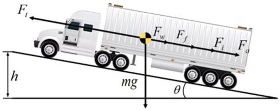
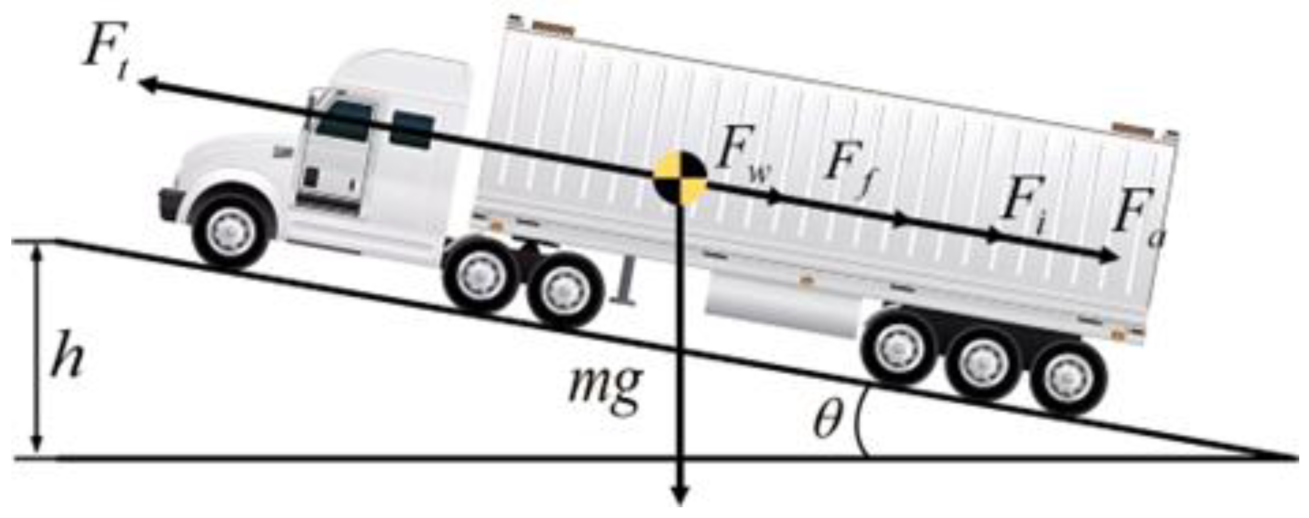
Finally, a single-degree-of-freedom vehicle dynamics model including only longitudinal movement is obtained, as shown in Figure 2.

Figure 2. Longitudinal force analysis of the vehicle. Note: The yellow-and-black circular marker in the figure indicates the center of gravity of the vehicle. The different colors are used only to visually highlight the location of the center of gravity and do not represent any additional physical meaning.

The above assumptions are mainly applicable to normal longitudinal driving conditions with limited tire slip and driveline dynamics. Under low-adhesion or rapid acceleration/braking conditions, tire slip and drive shaft deformation may cause deviations between the actual and modeled vehicle response, introducing errors into the kinematics-based road-gradient estimation and MPC state prediction. Although the GPS-based branch and IMM fusion can partially reduce the effect of model mismatch, these unmodeled dynamics cannot be completely eliminated.

According to Newton’s second law, the longitudinal acceleration of the vehicle can be expressed as follows:

$$m\cdot \ddot{s}(t)=F_t(t)-F_{air}(v(t))-F_{roll}(s(t))-F_g(s(t))$$

(4)

where $s$ is the distance when the vehicle is driving; $F_t(t)$ is the driving force; $F_{\mathrm{air}}=C_d\cdot A\cdot {\displaystyle \frac{1}{2}}\cdot \rho \cdot v^2$ is the air resistance, where $C_d$ is the air resistance coefficient, A is the area of the front end of the vehicle, $\rho$ is the air density, and v is the speed of the vehicle; $F_{\mathrm{roll}}=C_r\cdot m\cdot g$ is the rolling resistance, where $C_r$ is the rolling resistance coefficient, m is the mass of the vehicle, and g is the gravitational acceleration; and $F_{\mathrm{g}}(t)=m\cdot g\cdot \sin (\theta (t))$ is the gravitational resistance caused by the road slope, where $\theta (t)$ denotes the signed road-slope angle. The corresponding dimensionless road grade ratio is defined as $i=\tan \theta$. Under the small-slope assumption, with $\theta$ expressed in radians, $\sin \theta \approx \tan \theta =i$, and therefore $F_g\approx mgi$. For presentation, road-slope values are reported in degrees.

3. Energy Management Strategy Considering Road Gradient

3.1. Road Slope Estimation Based on IMM-KF

The longitudinal acceleration measured by the onboard sensor contains the actual longitudinal acceleration and the gravitational component induced by the road slope. In this study, $\theta$ denotes the signed road slope angle, while the dimensionless road grade ratio used in the estimator is defined as $i=\tan \theta$, where $i>0$, $i<0$, and $i=0$ correspond to uphill, downhill, and level roads, respectively. Under the small-slope assumption, with $\theta$ expressed in radians, $\sin \theta \approx \tan \theta =i$. Therefore, the measured longitudinal acceleration can be expressed as:

$$a_{senx}=a_x+gi$$

(5)

where $a_{senx}$ is the longitudinal acceleration measured by the onboard sensor, $a_x$ is the actual longitudinal acceleration, g is the local gravitational acceleration, and i is the dimensionless signed road grade ratio.

Differentiating Equation (5) gives the road grade variation rate as:

$$i^{\prime }=(a_{senx}^{\prime }-a_x^{\prime })/g$$

(6)

In the present implementation, the acceleration signals are first synchronized and preprocessed using an exponentially weighted moving average (EWMA) filter to suppress measurement noise and vibration-induced fluctuations. The road grade variation rate in Equation (6) is then calculated from the filtered acceleration signals before the Kalman filter prediction and measurement update steps. The calculated road grade rate signal is subsequently used as the input of the kinematics-based filtering branch. It is not obtained from the filtered road grade estimate and fed back into the same filter; therefore, no circular dependence is involved.

In the GPS-based estimation branch, the dimensionless road grade ratio at time k is calculated as:

$$i_{GPS}=\tan {\theta }_{GPS}={\displaystyle \frac{\Delta h}{\Delta s}}$$

(7)

where horizontal displacement $\Delta s=v\Delta t$, elevation change $\Delta h=h_k-h_{k-1}$, and $h_k$ denotes the elevation at time k.

The kinematics-based and GPS-based estimation methods are formulated within a unified state-space framework. The two filtering branches share the same state vector, state transition matrix, and measurement matrix, while the road grade information from the two estimation methods is introduced through the corresponding input terms. The state vector is defined as $x_k^{(j)}={[v_x(k),a_x(k),i{(k)}^{(j)}]}^T$, where $v_x$, $a_x$, and i denote the longitudinal vehicle speed, longitudinal acceleration, and dimensionless signed road grade ratio, respectively; and j = 1 and j = 2 denote the kinematics-based and GPS-based branches, respectively. The discrete state-space model is expressed as:

$$\left\{\begin{array}{l}{x}_k^{(j)}=A{x}_{k-1}^{(j)}+B_j{u}_{j,k}+{\omega }_k^{(j)},\\ z_k=H{x}_k+v_k,\end{array}\right. j=1,2$$

(8)

where the state-transition and measurement matrices are $A=\left[\begin{array}{ccc}1& \Delta t& 0\\ 0& 1-\delta \Delta t& g\\ 0& 0& 1\end{array}\right]$ and $H=[0,1,g]$, and the input matrices are explicitly specified as $B_1=B_2=I_3$, where $I_3$ denotes the 3 × 3 identity matrix. Here, $\Delta t=0.2 \mathrm{s}$ is the sampling interval, g = 9.81 m/s² is the gravitational acceleration, and $\delta =0.9$ is a fixed model parameter associated with the longitudinal-acceleration state transition. Specifically, $\delta$ appears through the coefficient $1-\delta \Delta t$, which determines the contribution of the previous acceleration state to the current state prediction. The parameter $\delta$ is independent of the IMM model probabilities and remains fixed throughout the estimation process.

For the kinematics-based branch, the road grade variation rate is obtained from Equation (6), and the corresponding input vector is $u_{1,k}={\left[0,0,{i^{\prime }}_{1,k}\Delta t\right]}^T$. For the GPS-based branch, the road grade ratio is calculated from the elevation change and horizontal displacement according to Equation (7), i.e., $i_{2,k}=\Delta h_k/\Delta s_k=\tan {\theta }_k$. The corresponding input vector is $u_{2,k}={\left[0,0,(\Delta h_k/\Delta s_k)\Delta t\right]}^T$. The two vectors therefore represent the respective input terms used by the kinematics-based and GPS-based Kalman filtering branches.

The measured longitudinal acceleration is used as the common observation for both filtering branches, i.e., $z_k=a_{senx,k}$. According to the small slope relationship in Equation (5), the measurement equation is:

$$a_{\mathrm{sen}x,k}=\left[\begin{array}{ccc}0& 1& g\end{array}\right]\left[\begin{array}{c}{v}_x(k)\\ a_x(k)\\ i(k)\end{array}\right]+v_k^{(j)}$$

(9)

The process and measurement noises satisfy $w_k^{(j)}~(0,Q_j)$ and $v_k^{(j)}~(0,R_j)$. The covariance parameters are set as $Q_1=\left[\begin{array}{ccc}2.5\times {10}^{-3}& 0& 0\\ 0& 1.0\times {10}^{-2}& 0\\ 0& 0& 9.0\times {10}^{-6}\end{array}\right]$, $Q_2=\left[\begin{array}{ccc}2.5\times {10}^{-3}& 0& 0\\ 0& 1.0\times {10}^{-2}& 0\\ 0& 0& 3.6\times {10}^{-5}\end{array}\right]$, and $R_1=R_2=1.0\times {10}^{-2}$. The initial covariance matrices are $P_1(0|0)=P_2(0|0)=\mathrm{diag}\left(0.25,0.04,4.0\times {10}^{-4}\right)$.

The IMM algorithm adaptively combines the two filtering branches according to their model probabilities. The Markov transition matrix and initial model probabilities are specified as $G=\left[\begin{array}{cc}0.95& 0.05\\ 0.05& 0.95\end{array}\right]$ and $\mu (0)=\left[\begin{array}{c}0.5\\ 0.5\end{array}\right]$, where $p_{ij}=P(M_k=j|M_{k-1}=i)$ denotes the transition probability from Model i to Model j. The predicted probability of Model j is calculated as:

$$c_j(k-1)={\displaystyle \sum _{i=1}^2{p}_{ij}}{\mu }_i(k-1)$$

(10)

The corresponding conditional mixing probability is

$${\mu }_{i|j}(k-1|k-1)={\displaystyle \frac{p_{ij}{\mu }_i(k-1)}{c_j(k-1)}}$$

(11)

After the Kalman update, the innovation is $r_j(k)=z_k-H{\widehat{x}}_j(k|k-1)$, and its covariance is $S_j(k)=H{P}_j(k|k-1)H^T+R_j$. Accordingly, the likelihood function is ${\Lambda }_j(k)={\displaystyle \frac{1}{\sqrt{2\pi S_j(k)}}}\exp \left[-{\displaystyle \frac{r_j^2(k)}{2S_j(k)}}\right]$.

The posterior model probability is updated as

$${\mu }_j(k)={\displaystyle \frac{{\Lambda }_j(k)c_j(k-1)}{\eta (k)}},\hspace{1em}\eta (k)={\displaystyle \sum _{j=1}^2{\Lambda }_j}(k)c_j(k-1)$$

(12)

Finally, the fused state estimate is obtained by probability-weighted averaging of the two filtering results:

$$\widehat{x}(k|k)={\displaystyle \sum _{j=1}^2{\mu }_j}(k){\widehat{x}}_j(k|k)$$

(13)

When GPS measurements become unreliable, the IMM likelihood update reduces the probability of the GPS-based branch, thereby increasing the contribution of the kinematics-based estimate. In practical implementation, complete GPS dropout can be handled by suspending the GPS measurement update and temporarily relying on the kinematics-based branch until valid GPS data are restored. This prevents unavailable GPS information from directly affecting the fused estimate; however, prolonged GPS outages may still increase estimation uncertainty due to sensor bias and model errors.

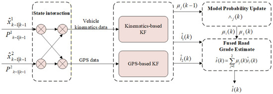
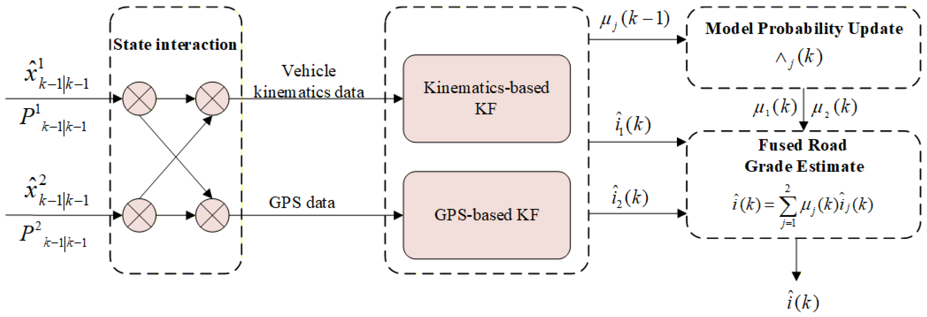
The architecture of the road slope estimation algorithm obtained is shown in Figure 3.

Figure 3. Simplified architecture of the IMM-KF road grade estimation framework. Note: The Arrows indicate information flow, dashed boxes denote functional modules, and background colors are used only for visual distinction. The symbols are defined in the corresponding equations and text.

As shown in Figure 3, the IMM-KF road grade estimation framework consists of state interaction, two parallel Kalman filtering branches, model probability update, and road grade fusion. The kinematics-based KF estimates the road grade using vehicle kinematics data, while the GPS-based KF provides an independent estimate using GPS data. Based on the model likelihood $\Lambda j\left(k\right)$ and the prior model probability ${\mu }_j\left(k-1\right)$, the model probabilities are updated to ${\mu }_1\left(k\right)$ and ${\mu }_2\left(k\right)$. The two road grade estimates, ${\widehat{i}}_1\left(k\right)$ and ${\widehat{i}}_2\left(k\right)$, are then weighted by their corresponding model probabilities to obtain the final fused road grade estimate. The state estimates obtained at the current sampling step are subsequently used in the state interaction process for the next estimation cycle. It should be emphasized that the IMM-KF developed in this section estimates the road grade at the current vehicle position from available onboard measurements. It does not independently predict the future road gradient sequence required over the MPC prediction horizon.

3.2. Economic Vehicle Speed Planning Based on Model Predictive Control

The longitudinal motion of the vehicle is governed by the balance between the driving force and the resistance forces. The standard longitudinal dynamics equation is first written as:

$$m\dot{v}(t)=F_t(t)-F_r(t)-F_a(t)-F_g(t)$$

(14)

where m is the vehicle mass and Ft is the longitudinal driving force. The rolling resistance, aerodynamic drag, and grade resistance are respectively defined as $F_r(t)=mgf\cos \theta (s(t))$, $F_a(t)={\displaystyle \frac{1}{2}}\rho C_{D}A{v}^2(t)$, and $F_g(t)=mg\sin \theta (s(t))$, where f is the rolling resistance coefficient, g is the gravitational acceleration, $\rho$ is the air density, C_D is the aerodynamic drag coefficient, A is the frontal area of the vehicle, and $\theta (s)$ is the road gradient angle at position s.

For the MPC formulation, the vehicle position and longitudinal speed are selected as the state variables, i.e., $x(t)={\left[\begin{array}{cc}s(t)& v(t)\end{array}\right]}^T$, and the driving force $F_t(t)$ is selected as the control input. Substituting the resistance forces into the longitudinal dynamics equation gives the nonlinear state-space model

$$\dot{x}(t)=\left[\begin{array}{l}\dot{s}(t)\\ \dot{v}(t)\end{array}\right]=\left[\begin{array}{l}v(t)\\ {\displaystyle \frac{F_t(t)}{m}}-gf\cos \theta (s(t))-{\displaystyle \frac{C_D\rho A{v}^2(t)}{2}}-g\sin \theta (s(t))\end{array}\right]$$

(15)

This state-space model is subsequently used as the prediction model in the MPC framework for vehicle state prediction and driving force optimization.

Therefore, the state-space model of the system can be expressed as follows:

$$\dot{x}(t)=f(x(t),u(t),t)$$

(16)

where $u(t)=F_t(t)$ denotes the control input.

Conventional model predictive control (MPC) generally performs state prediction in the time domain, while road slope is a spatially varying parameter closely related to vehicle position. Time-domain prediction models cannot accurately reflect the influence of future road grade on vehicle dynamics. Therefore, the vehicle dynamic model is transformed from the time domain into the spatial domain to improve the adaptability of vehicle speed planning to road conditions.

The relationship between vehicle position and velocity is expressed as:

$${\displaystyle \frac{ds}{dt}}=v$$

(17)

Using the chain rule, the vehicle acceleration can be transformed into the spatial domain as:

$${\displaystyle \frac{dv}{ds}}={\displaystyle \frac{a}{v}}$$

(18)

Combining the longitudinal vehicle dynamics equation, the spatial-domain vehicle model can be obtained as:

$$m\cdot {\displaystyle \frac{dv}{ds}}\cdot v=F_{\mathrm{total}}-F_{\mathrm{r}}$$

(19)

In the formula: m represents the mass of the vehicle, v represents the speed of the vehicle, s represents the position of the vehicle, $F_{\mathrm{total}}$ represents the resultant external force acting on the vehicle, and $F_{\mathrm{r}}$ represents the resultant resistance force.

Through the above transformation, the MPC can incorporate road gradient information over its spatial prediction horizon. In the present simulation study, however, the future gradient sequence is not predicted online by the IMM-KF. Instead, the complete real road gradient profile is reconstructed beforehand from the recorded road data, transformed into the spatial domain, interpolated at equal spatial intervals, and stored as route-based gradient data. At each MPC update, the gradient sequence corresponding to the upcoming prediction horizon is extracted from this stored profile. Therefore, the present MPC simulations assume ideal availability of route gradient preview information.

The longitudinal dynamics model contains nonlinear terms, particularly the quadratic aerodynamic drag term. To reduce the computational burden of the MPC, the longitudinal force balance equation is transformed into an energy-based model in the spatial domain. Considering the rotational inertia of the vehicle components, the equivalent vehicle mass is represented by $\delta m$, where $\delta$ is the rotational mass conversion coefficient. Using the spatial relationship $a=vdv/ds$ and multiplying the force balance equation by the traveling distance $\Delta s$, the change in vehicle kinetic energy over one spatial interval can be expressed as

$${\displaystyle \frac{\delta m{v}^2(s+\Delta s)}{2}}={\displaystyle \frac{\delta m{v}^2(s)}{2}}-{\displaystyle \frac{C_D\rho A{v}^2(s)\Delta s}{2}}+\left(F_t(s)-mgf\cos \theta (s)-mg\sin \theta (s)\right)\Delta s$$

(20)

Defining the equivalent kinetic energy as $E(s)={\displaystyle \frac{1}{2}}\delta m{v}^2(s)$, the quadratic velocity term in Equation (19) can be replaced by $v^2(s)={\displaystyle \frac{2E(s)}{\delta m}}$. The road is then divided into equally spaced segments of length $\Delta s$, with $s_k=k\Delta s$. Assuming that the driving force and road gradient remain constant within each short spatial interval, Equation (19) can be discretized as

$$E(k+1)=\left(1-{\displaystyle \frac{C_D\rho A}{\delta m}}\Delta s\right)E(k)+\Delta s{F}_t(k)-\Delta s\left[\begin{array}{cc}mgf& mg\end{array}\right]\left[\begin{array}{c}\cos \theta (k)\\ sin\theta (k)\end{array}\right]$$

(21)

Therefore, the spatial-domain energy model can be written in the standard state-space form as

$$x\left(k+1\right)=Ax\left(k\right)+B_{u}u\left(k\right)+B_{d}d\left(k\right)$$

(22)

For the MPC formulation, the kinetic energy is selected as the state variable, the driving force as the control variable, and the road gradient terms as measurable disturbances:

$$\left\{\begin{array}{l}x(k)=E(k)\hfill \\ u(k)=F_t(k)\hfill \\ d(k)=\left[\begin{array}{c}\cos \theta (k)\\ \sin \theta (k)\end{array}\right]\hfill \end{array}\right.$$

(23)

Accordingly, the matrices in Equation (21) are

$$\left\{\begin{array}{l}A=1-{\displaystyle \frac{C_D\rho A}{\delta m}}\Delta s\hfill \\ B_u=\Delta s\hfill \\ B_d=-\Delta s\left[mgf\hspace{1em}mg\right]\hfill \end{array}\right.$$

(24)

This energy-domain formulation eliminates the quadratic speed term from the prediction model and is therefore more suitable for repeated optimization in the MPC. The reference kinetic energy is calculated from the reference vehicle speed as $E_{\mathrm{ref}}(k)={\displaystyle \frac{1}{2}}\delta m{v}_{\mathrm{ref}}^2(k)$. The MPC objective function is defined as

$$J={\displaystyle \sum _{k=1}^p\left[{\beta }_1{\left(E(k)-E_{\mathrm{ref}}(k)\right)}^2+{\beta }_2{\left(F_t(k)\Delta s\right)}^2\right]}$$

(25)

where p is the prediction horizon, and ${\beta }_1$ and ${\beta }_2$ are weighting coefficients. The first term penalizes the deviation of the vehicle kinetic energy from that corresponding to the reference speed, thereby maintaining the desired traffic efficiency. In the second term, $F_t(k)\Delta s$ represents the longitudinal driving work required over the k-th spatial interval. Therefore, this term penalizes excessive driving-energy demand and control effort. The two terms jointly balance reference speed tracking and energy demand during the MPC optimization. Here, the driving work term is used as an energy-oriented surrogate for fuel consumption to maintain computational tractability; therefore, some fuel optimality loss may exist compared with a nonlinear fuel-map-based MPC, although this loss cannot be quantitatively isolated without a direct benchmark.

To ensure the feasibility of the MPC optimization and maintain the vehicle within its allowable operating range, constraints are imposed on the vehicle speed, longitudinal acceleration, and driving force as follows:

$$\left\{\begin{array}{c}{v}_{\min }\le v\le v_{\max }\\ a_{\min }\le a\le a_{\max }\\ F_{\min }\le F_t\le F_{\max }\end{array}\right.$$

(26)

The constraint bounds used in this study are $v_{\min }=0 \mathrm{m}/\mathrm{s}$, $v_{\max }=30 \mathrm{m}/\mathrm{s}$, $a_{\min }=-3 {\mathrm{m}/\mathrm{s}}^2$, $a_{\max }=2 {\mathrm{m}/\mathrm{s}}^2$, $F_{\min }=-4000 \mathrm{N}$, and $F_{\max }=4000 \mathrm{N}$. The speed and acceleration constraints maintain the vehicle within the prescribed operating range, while the driving-force constraint limits the control input to the admissible longitudinal force range.

3.3. Optimization of Adaptive Energy Management Strategy Based on Particle Swarm

The energy consumption model converts battery energy consumption into equivalent fuel consumption by using an equivalent factor. The objective of the strategy is to minimize the total equivalent energy consumption of all power sources over a given time or distance. It also ensures that the battery SOC remains within a reasonable range.

The cost function J, based on the equivalent fuel consumption model, can be expressed as follows:

$$J={\displaystyle {\int }_{t_0}^{t_f}({\dot{m}}_{eng}(T_e,n_e)+{\dot{m}}_{mot}(T_m,n_m))}dt+f(so{c}_{(t_f)})$$

(27)

In the equation, t₀ and t_f represent the initial and terminal moments of the driving cycle, respectively; ${\dot{m}}_{eng}(T_e,n_e)$ denotes the instantaneous fuel consumption of the engine, which is determined by the engine torque $T_e$ and rotational speed $n_e$; ${\dot{m}}_{mot}(T_m,n_m)$ signifies the equivalent fuel consumption of the electric motor, dependent on the motor torque $T_m$ and rotational speed $n_m$; and $f(so{c}_{(t_f)})$ is a penalty function associated with the battery state of charge (SOC), designed to penalize deviations from the target SOC at the cycle’s conclusion, thereby ensuring the SOC remains within the predefined range.

To ensure that the control and state variables satisfy operational requirements and maintain system feasibility, the parameters of the vehicle dynamics model are constrained as follows:

$$\left\{\begin{array}{l}{T}_{e\text{\_}\min }(n_e(t))\le T_e(t)\le T_{e\text{\_}\max }(n_e(t))\\ n_{e\text{\_}\min }\le n_e(t)\le n_{e\text{\_}\max }\\ T_{m\text{\_}\min }(n_m(t))\le T_m(t)\le T_{m\text{\_}\max }(n_m(t))\\ n_{m\text{\_}\min }\le n_m(t)\le n_{m\text{\_}\max }\\ SO{C}_l\le SOC(t)\le SO{C}_h\end{array}\right.$$

(28)

In Equation (28), $T_e(t)$ represents the engine torque; $T_{e\text{\_}\min }(n_e(t))$ and $T_{e\text{\_}\max }(n_e(t))$ denote the minimum and maximum output torque of the engine at speed $n_e(t)$, respectively; $n_{e\text{\_}\min }$ and $n_{e\text{\_}\max }$ indicate the lower and upper limits of the engine speed; $T_m(t)$ signifies the motor torque; $T_{m\text{\_}\min }(n_m(t))$ and $T_{m\text{\_}\max }(n_m(t))$ represent the minimum and maximum output torque of the motor at speed $n_m(t)$, respectively; $n_{m\text{\_}\min }$ and $n_{m\text{\_}\max }$ denote the lower and upper limits of the motor speed; $SOC(t)$ represents the SOC of the battery; and $SO{C}_l$ and $SO{C}_h$ indicate the minimum and maximum SOC limits of the battery, respectively.

The battery SOC is selected as the state variable. For a given vehicle power demand, the engine torque $T_e$ is treated as the independent control decision, while the corresponding motor torque $T_m$ is determined according to the power-balance relationship. Thus, $T_e$ and $T_m$ constitute the engine motor power split pair, but only one independent control degree of freedom remains after enforcing the instantaneous power-balance constraint. The Hamiltonian function based on Pontryagin’s Minimum Principle (PMP) is expressed as follows:

$$H={\dot{m}}_{eqv}(t)+\lambda (t)\cdot S\dot{O}C(t)$$

(29)

In Equation (29), ${\dot{m}}_{eqv}(t)$ represents the instantaneous equivalent fuel consumption; $\lambda (t)$ denotes the co-state variable, indicating the influence of SOC on the objective function; and $S\dot{O}C(t)$ signifies the rate of change in battery SOC, typically determined by motor power and battery characteristics. The Hamiltonian function can be further expressed as:

$$H={\dot{m}}_{eqv}(t)+s{\displaystyle \frac{P_{bat}(t)}{H_{LHV}}}$$

(30)

where s is the equivalence factor, $P_{bat}(t)$ is the battery power, and $H_{LHV}$ is the lower heating value of the fuel.

According to PMP, at each control step, the feasible engine torque $T_e$ is discretely searched within its allowable range. For each candidate $T_e$, the corresponding motor torque $T_m$ is determined from the instantaneous vehicle power-balance relationship. Candidate engine motor torque pairs that violate the component or battery constraints are excluded. The Hamiltonian is then evaluated for each feasible torque pair, and the pair yielding the minimum Hamiltonian is selected as the optimal control action.

$$\left[{T^{\ast }}_{e,opt}(t),{T^{\ast }}_{m,opt}(t)\right]=\arg \min H$$

(31)

After obtaining the optimal control inputs, the battery SOC is updated according to the battery power, thereby realizing the online energy management of the A-ECMS.

The feasible engine motor torque pair corresponding to the minimum Hamiltonian is selected as the optimal power-split solution.

$$SOC(t+1)=SOC(t)+S\dot{O}C(t)\cdot \Delta t$$

(32)

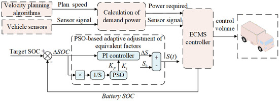
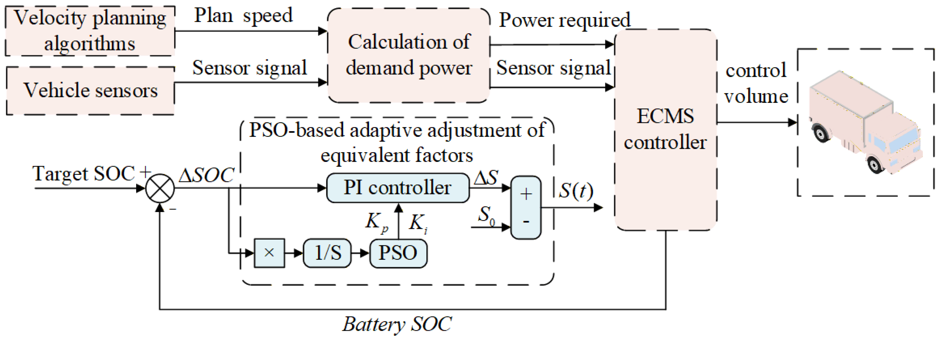
At present, the adaptive equivalent consumption minimization strategy (A-ECMS) is mostly based on the PI controller and adjusts the equivalent factor through battery SOC feedback [35]. Its control framework is shown in Figure 4.

Figure 4. A-ECMS vehicle control strategy architecture. Note: Arrows indicate signal flow, colored backgrounds distinguish different functional modules, dotted boxes group the corresponding modules, and the summation symbol represents the calculation of the SOC deviation between the target and actual SOC.

The conventional A-ECMS adjusts the equivalence factor through SOC feedback using a PI controller. Because the PI gains are usually selected empirically, PSO is employed offline in this study to calibrate these gains. The resulting strategy is referred to as PA-ECMS, as shown in Figure 5. In this strategy, the PI controller parameters $[K_p,K_i]$ in A-ECMS are optimized offline using the PSO algorithm.

Figure 5. PA-ECMS architecture diagram based on particle swarm optimization. Note: Arrows indicate signal flow, colored backgrounds distinguish different functional modules, dotted boxes group the corresponding modules, and the summation symbol represents the calculation of the SOC deviation between the target and actual SOC.

The online equivalent factor adjustment follows the SOC feedback PI formulation:

$$s(t)=s_0+K_p[SO{C}_{t\arg et}-SOC(t)]+K_i{\displaystyle {\int }_0^t(}SO{C}_{t\arg et}-SOC(t))dt$$

(33)

where $s_0$ denotes the initial equivalent factor, and $K_p$ and $K_i$ are the proportional and integral gains optimized by PSO. During online operation, the vehicle power demand is considered in the ECMS Hamiltonian optimization to determine the engine–motor power split, rather than directly modifying the equivalent factor.

During the PSO process, each particle position represents a set of PI controller parameters. The search range of $K_p$ is set to [1, 20], while the search range of $K_i$ is set to [0.1, 1]. First, the particle positions and velocities are randomly initialized. Then, the A-ECMS is executed under the given driving cycle, and the equivalent fuel consumption of the vehicle is used as the fitness function for evaluation. Subsequently, the particle velocities and positions are iteratively updated according to both the individual best solution and the global best solution. Meanwhile, the parameter boundaries and velocity ranges are constrained to ensure the stability and feasibility of the optimization process. After multiple iterations, the optimal PI parameter combination is obtained when the fitness function converges. In this study, the population size is set to 10, and the maximum number of iterations is set to 100.

The optimized PI parameters are then applied to the online adaptive adjustment of the equivalent factor in A-ECMS. Compared with conventional A-ECMS, the proposed strategy reduces the dependence on empirical PI parameter selection through PSO-based offline calibration. During online operation, the equivalent factor is adjusted according to SOC deviation, while the instantaneous power demand is considered in the ECMS optimization to determine the optimal engine motor power distribution.

The equivalent factor is adaptively adjusted based on the deviation between the current and target SOC, while vehicle power demand is considered during the ECMS power allocation process. Since the PSO-optimized PI parameters remain fixed during online operation, variations in payload or driving profiles may affect the optimal calibration. The robustness under these conditions has not been explicitly evaluated in the present study.

The main implementation parameters of the MPC and PA-ECMS strategies are summarized in Table 3. For the spatial-domain MPC, a prediction horizon of p = 40 and a spatial discretization step of $\Delta s = 10$ m correspond to a physical road-gradient preview distance of 400 m.

Table 3. Main implementation parameters of the MPC and PA-ECMS strategies.

Category	Parameter	Value
MPC	Prediction horizon, p	40
	Spatial discretization step, Δs	10 m
	Physical preview distance, Lp = pΔs	400 m
	Kinetic-energy tracking weight, Q	0.1
	Control-input weight, R	1
	Optimization solver	MATLAB quadprog
PSO	Population size	10
	Maximum iterations	100
	Cognitive coefficient, c1	1.49445
	Social coefficient, c2	1.49445
	Search range of Kp	[1, 20]
	Search range of Ki	[0.1, 1]
	Velocity range of Kp	[−1, 1]
	Velocity range of Ki	[−0.1, 0.1]
	Optimized Kp	18.3990
	Optimized Ki	0.8130

3.4. Computational Complexity and Simulation-Based Feasibility Analysis

In the proposed framework, the IMM-KF-based road gradient estimator mainly involves state interaction and Kalman filtering with a relatively low dimensional state vector, resulting in a relatively low computational complexity. For the upper-layer controller, the MPC-based economic speed-planning strategy adopts a finite prediction horizon of 40 to balance optimization performance and computational complexity. The optimization variables are limited to the longitudinal vehicle states, and a constrained optimization problem is solved at each control step. In the lower-layer energy management strategy, PSO is only used offline to optimize the PI controller parameters and therefore does not introduce additional online computational burden. During online operation, the PA-ECMS mainly performs equivalent factor adjustment and Hamiltonian minimization over a discretized control set. These characteristics indicate the computational feasibility of the proposed framework in the present MATLAB/Simulink simulations. However, no hardware-level timing evaluation is conducted in this study. Therefore, actual execution time, communication delay, actuator dynamics, and embedded real-time performance should be further evaluated through hardware-in-the-loop and real vehicle experiments.

4. Validation and Results

4.1. Verification of Road Slope Estimation

To evaluate the accuracy and adaptability of the road slope estimation model, real-road vehicle operation data were collected using an XTOOL H6Pro (Shenzhen XTOOLTECH Co., Ltd., Shenzhen, China) and a VK162-GPS device. The XTOOL H6Pro was connected to the vehicle OBD interface to acquire longitudinal acceleration signals, while the VK162-GPS was used to record vehicle position, speed, and altitude information. Both devices operated at a sampling frequency of 10 Hz, and all signals were synchronized according to a unified time reference to ensure data consistency.

The reference road gradient profile was constructed from GPS-based elevation and traveled distance information. After removing abnormal measurements and reducing noise, the elevation variation between adjacent GPS points was converted into gradient values. Since the original gradient samples were discrete in the spatial domain, interpolation was performed according to traveled distance to obtain a continuous reference profile for evaluating the proposed slope estimation method.

To quantitatively assess the performance of different algorithms, two commonly used metrics, mean absolute error (MAE) and root mean square error (RMSE), were adopted. MAE represents the average deviation between the estimated and reference values, while RMSE gives greater weight to larger estimation errors.

(1)

Constant-gradient condition

The constant-gradient condition corresponds to a relatively stable road segment with a length of approximately 1500 m and only minor slope variations. This experiment can effectively eliminate the influence of complex external factors on model accuracy, thereby enabling validation of the fundamental performance of the proposed model under relatively ideal conditions.

To verify the accuracy of the proposed road grade estimation model, the longitudinal road gradient was measured at intervals of 10 m using a SNDWAY SW-LR180 (Sndway Technology (Guangdong) Co., Ltd., Dongguan, China) digital level with an angular measurement accuracy of ±0.1° within the measurement range considered in this study. The discrete measurements were subsequently interpolated to obtain the reference road-gradient profile of the experimental road section.

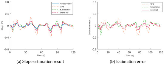
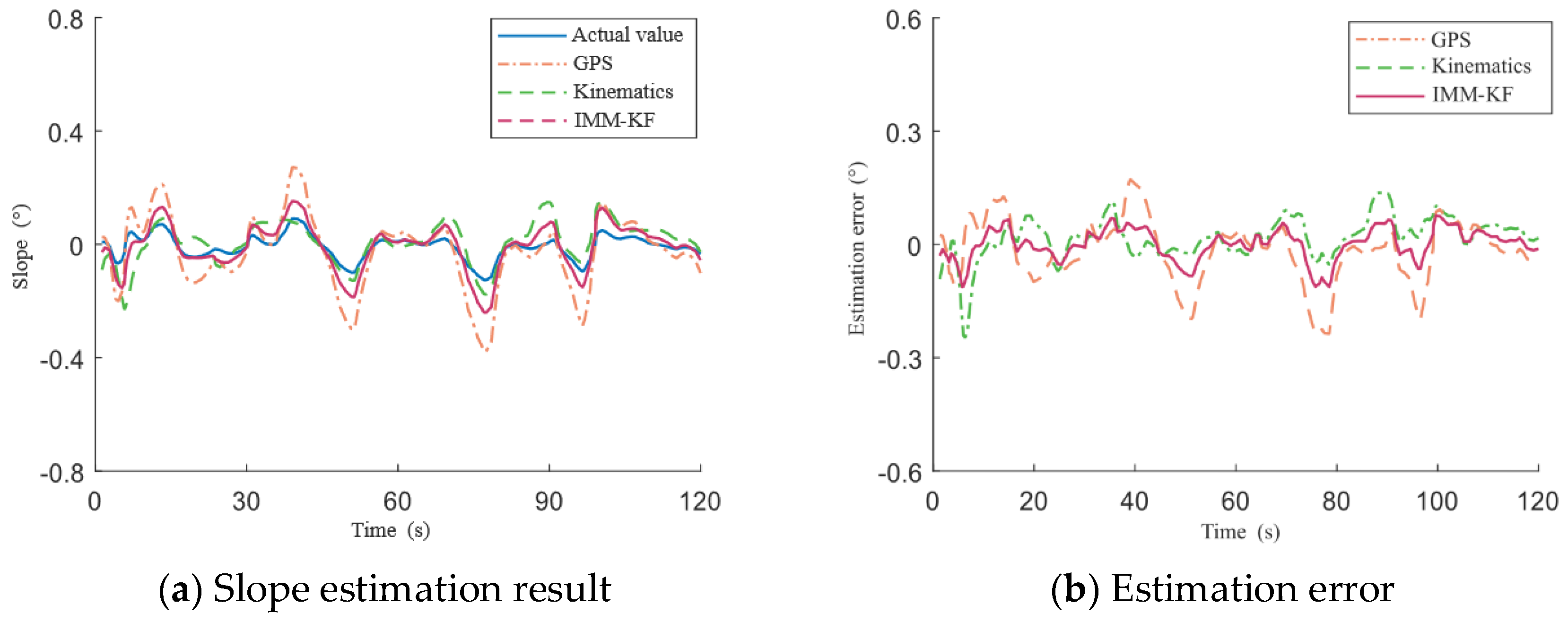
Figure 6 illustrates the estimation results and error variations of the kinematics-based road grade estimation model, the GPS-based road grade estimation model, and the proposed IMM-KF model under the constant-gradient condition. As shown in Figure 6a, the road grade curve estimated by the IMM-KF model is generally more consistent with the actual road grade profile. Compared with the kinematics-based and GPS-based estimation methods, the proposed model can more accurately capture the variation trend of the road grade.

Figure 6. Slope estimation results and errors under constant-gradient conditions.

Furthermore, the estimation error curves shown in Figure 6b indicate that the IMM-KF model exhibits smaller overall fluctuations and remains closer to zero compared with the other two models. This demonstrates that the proposed model achieves higher estimation accuracy and stronger robustness, effectively reducing error accumulation while stably tracking the actual road grade.

The calculated error metrics of different models under the constant-gradient condition are presented in Table 4. It can be observed that the MAE and RMSE values of all three models are relatively small under stable road conditions, indicating that the three road grade estimation models can accurately estimate road grade when the slope variation is small or nearly constant. Among them, the IMM-KF-based estimation method achieves lower MAE and RMSE values than the kinematics-based and GPS-based estimation methods, demonstrating the superiority of the proposed model in terms of estimation accuracy and robustness.

Table 4. Error metric results of slope estimation under constant-gradient conditions.

Slope Estimation Methods	MAE (°)	RMSE (°)
Slope estimation based on GPS	0.06815	0.08977
Slope estimation based on kinematic model	0.04623	0.06405
Slope estimation based on IMM-KF	0.03492	0.04461

(2)

Variable-Gradient Slope Estimation Performance

The experimental road has a total length of approximately 4 km and includes multiple typical driving conditions, including flat roads, continuous uphill sections, continuous downhill sections, and multi-stage slope transition regions. The overall road mainly consists of mild slopes while containing several local sections with relatively large slope variations, which can effectively reflect realistic longitudinal road load characteristics and validate the robustness and adaptability of the proposed energy management strategy under complex road conditions. According to the road grade estimation results, the road slope angle ranges approximately from −8° to +8°, covering flat, uphill, and downhill driving conditions.

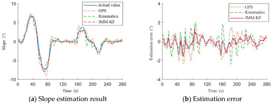
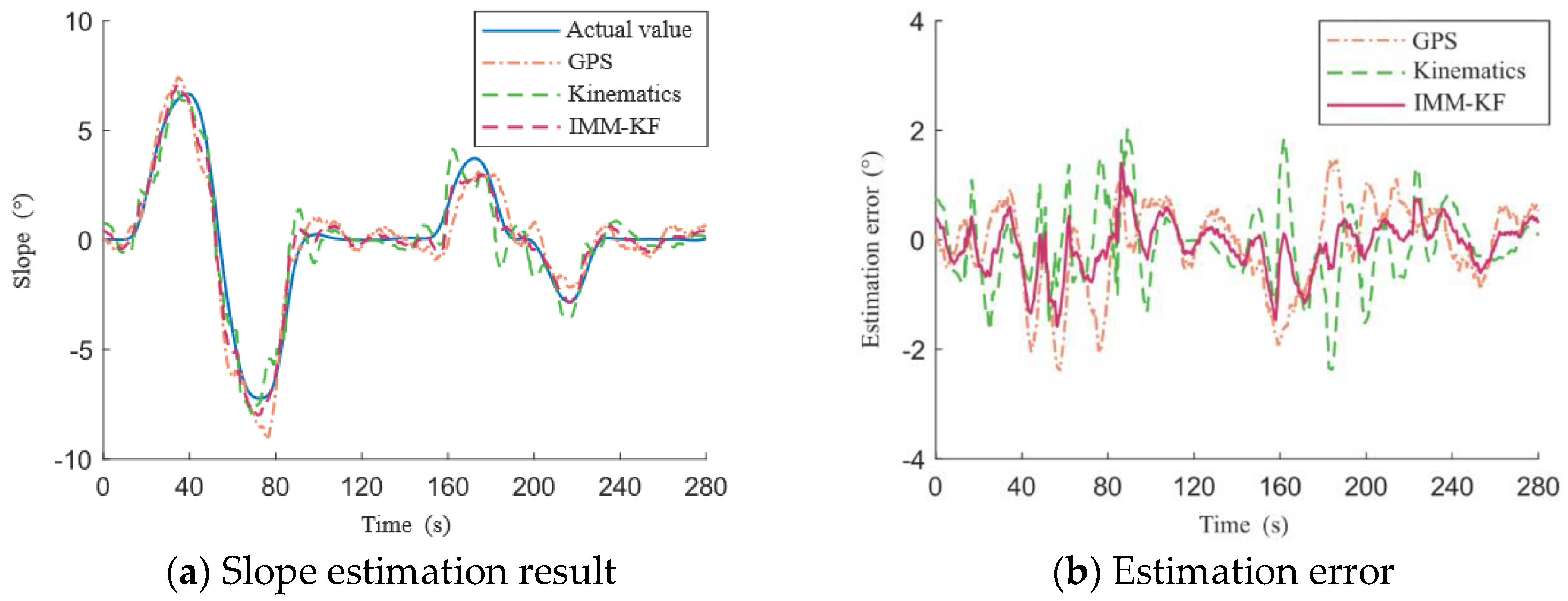
Figure 7 illustrates the estimation performance and error variations of the kinematics-based gradient estimation model, the GPS-based gradient estimation model, and the proposed IMM-KF model under actual variable gradient driving conditions.

Figure 7. Slope estimation results and errors under actual working conditions.

As shown by the estimation curves in Figure 7a, when the road gradient varies significantly, the GPS-based estimation model exhibits a noticeable response delay, while the kinematics-based model shows certain oscillations. In contrast, the IMM-KF model achieves rapid convergence to the true gradient, indicating strong adaptability and robustness. Moreover, it yields smoother transitions and reduced estimation errors at uphill–flat transition regions compared with the other models.

As shown by the estimation error curves in Figure 7b, the estimation errors of all three models are generally maintained within 2°, satisfying the accuracy requirements. Compared with the GPS-based and kinematics-based models, the IMM-KF model exhibits reduced fluctuation frequency and amplitude, further demonstrating its effectiveness in improving gradient estimation accuracy.

The calculated error metrics under variable-gradient driving conditions are summarized in Table 5. In terms of mean absolute error (MAE), the IMM-KF model achieves a value of 0.35592, which is lower than those of the kinematics-based model (0.54779) and the GPS-based model (0.62483), indicating reduced estimation error and improved accuracy. Similarly, with respect to the root mean square error (RMSE), the IMM-KF model also exhibits a lower value than the other two estimation methods, further demonstrating its superior overall performance.

Table 5. The calculation results of error indicators under actual operating conditions.

Slope Estimation Methods	MAE (°)	RMSE (°)
Slope estimation based on GPS	0.62483	0.78919
Slope estimation based on kinematic model	0.54779	0.71522
Slope estimation based on IMM-KF	0.35592	0.47587

These results indicate that the IMM-KF method exhibits stronger robustness in handling dynamically varying road gradient information. It effectively reduces the occurrence of large estimation errors and improves overall estimation accuracy. Consequently, the IMM-KF model can stably track actual road gradient variations under complex and time-varying driving conditions, further confirming its enhanced adaptability and estimation precision.

4.2. Validation of Economic Speed Planning

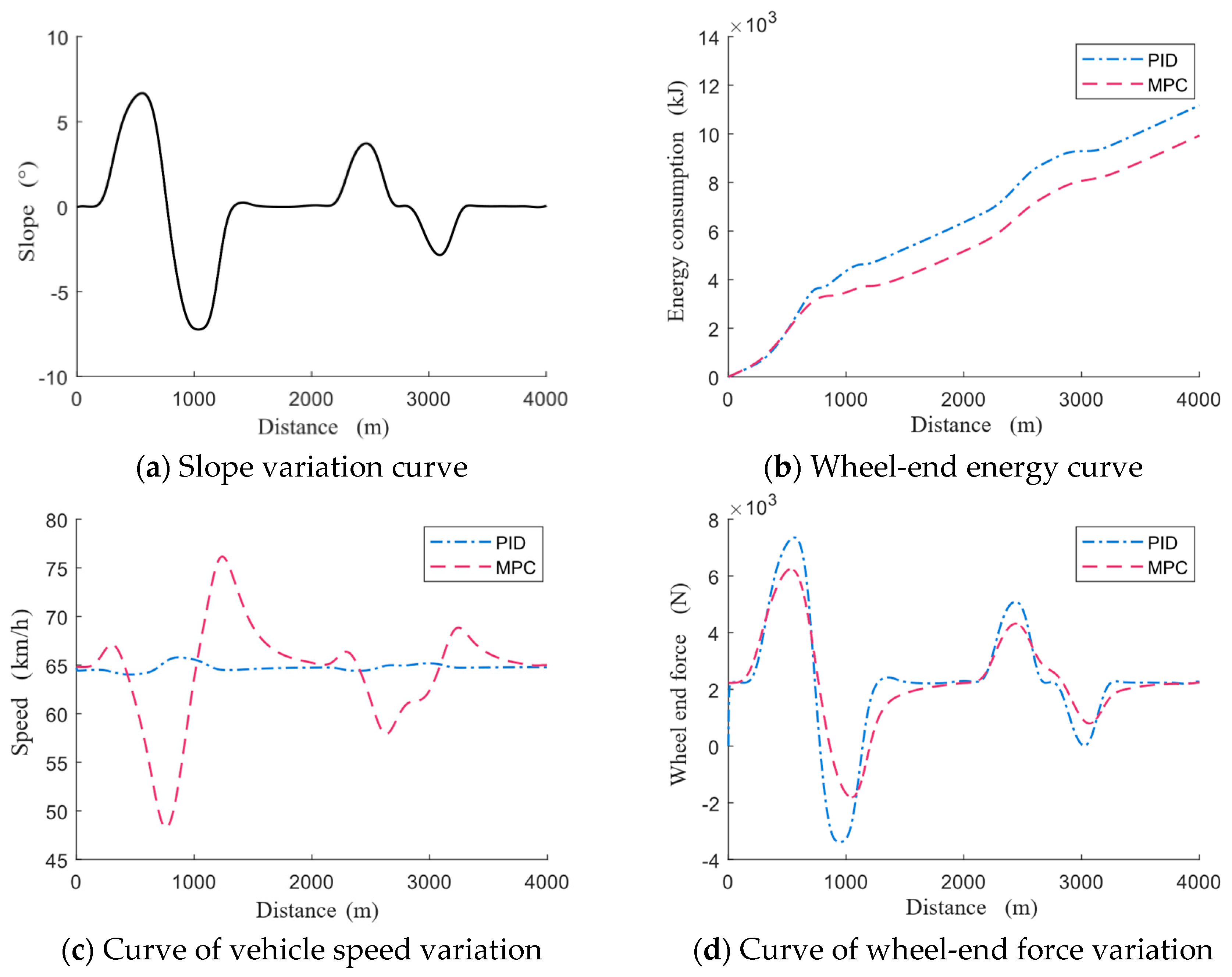
To evaluate the proposed economic speed-planning algorithm under real road conditions, the recorded road data are first processed using the road gradient estimation framework and converted into a spatial domain road gradient profile. For the MPC simulation, this complete profile is stored in advance and the gradient sequence over each prediction horizon is extracted according to the current vehicle position. Thus, the simulation assumes ideal availability of the route gradient preview rather than online prediction of future road grade by the IMM KF. The proposed MPC-based speed-planning algorithm is tested and compared with a conventional PID-based cruise control strategy. This comparison is used to isolate the contribution of the upper-layer economic speed-planning strategy before considering differences in lower-layer power-split control.

The real road segment has a total length of approximately 4 km, and the target cruising speed is set to 65 km/h. The vehicle speed is constrained within 0–30 m/s, and the longitudinal acceleration is limited to −3–2 m/s². The MPC prediction horizon is set to p = 40. Accordingly, at each optimization step, 40 successive road gradient samples are obtained from the pre-stored spatial road profile and supplied to the MPC as preview disturbances.

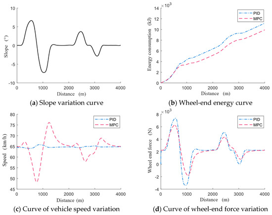
Figure 8 presents the simulation results of different control algorithms under real-road driving conditions. As observed from Figure 8a,c, the PID-based cruise control system continuously tracks the preset cruising speed without considering road gradient variations. As a result, during uphill driving, the vehicle passively decelerates due to gravitational resistance and subsequently increases power output to recover the target speed, leading to additional energy consumption. During downhill driving, the vehicle speed tends to increase as potential energy is converted into kinetic energy, and braking is required to regulate the speed, which results in energy dissipation.

Figure 8. Simulation results of the speed-planning algorithm for actual road conditions.

In contrast, the proposed MPC-based algorithm dynamically adjusts the vehicle speed according to road gradient information. The vehicle performs pre-acceleration before uphill sections to mitigate gradient-induced resistance. This strategy helps avoid unnecessary traction energy demand associated with subsequent speed recovery. Similarly, the vehicle decelerates in advance before downhill sections to limit excessive speed increases, thereby reducing energy losses associated with frequent braking. Consequently, the vehicle speed profile exhibits moderate fluctuations. As shown by the wheel-end energy curves in Figure 8b, compared with the PID-based cruise control strategy, the proposed algorithm reduces the total wheel-end energy demand, indicating improved energy efficiency at the vehicle level.

To further quantitatively analyze the differences between the two algorithms, the detailed simulation results under real-road driving conditions are summarized in Table 6. It can be observed that the vehicle equipped with the PID-based cruise control system achieves an average speed of 64.79 km/h, while the vehicle using the proposed algorithm attains an average speed of 64.50 km/h. Both average speeds are close to the preset cruising speed of 65 km/h, indicating that the proposed strategy satisfies the requirements for transportation efficiency.

Table 6. Simulation comparison results of two algorithms under actual road conditions.

Strategy	PID	MPC
Average vehicle speed (km/h)	64.79	64.50
Average wheel end force (N)	2272.93	2277.24
Total wheel end energy (kJ)	11,139.38	9916.13
Wheel-end energy reduction (%)	/	10.98

However, in terms of wheel-end energy consumption, under the condition of similar average wheel-end force values, the proposed MPC-based speed-planning algorithm demonstrates superior energy-saving performance. The wheel-end energy consumption of the proposed method is 9916.13 kJ, which is significantly lower than the 11,139.38 kJ consumed by the PID-based strategy, corresponding to a reduction of up to 10.98%. These results demonstrate that the proposed MPC-based algorithm effectively reduces wheel-end energy demand through rational speed adjustment during uphill and downhill driving while maintaining similar transportation efficiency. The 10.98% reduction reported here refers specifically to wheel-end energy consumption and should not be interpreted as an equivalent reduction in fuel consumption.

4.3. Validation of Energy Management Strategy

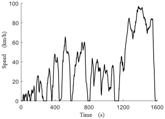
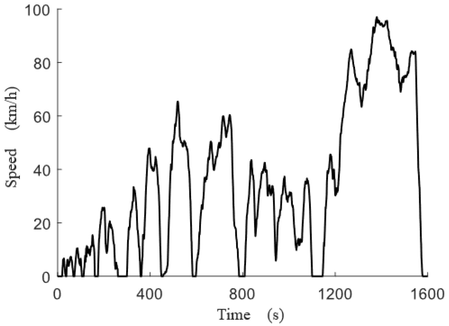
To evaluate lower-layer energy management, PA-ECMS, A-ECMS, and offline DP are tested under the same prescribed CHTC-LT speed trajectory shown in Figure 9. The PI parameters of PA-ECMS are calibrated offline by PSO on this same cycle. In DP, SOC is the state variable, engine power is the control variable, and motor power follows the power balance; thus, DP optimizes only the lower-layer power split rather than vehicle speed. SOC variation and comprehensive operating cost are used as performance metrics. No road gradient preview is introduced in this lower-layer comparison. For the DP benchmark, the initial and reference SOC are both set to 0.50, the SOC is constrained within [0.40, 0.60], and charge sustenance is encouraged through a terminal SOC penalty rather than by enforcing an identical terminal SOC value.

Figure 9. Speed profile of the CHTC-LT driving cycle.

(1)

Vehicle Speed Tracking Performance

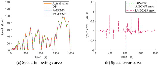
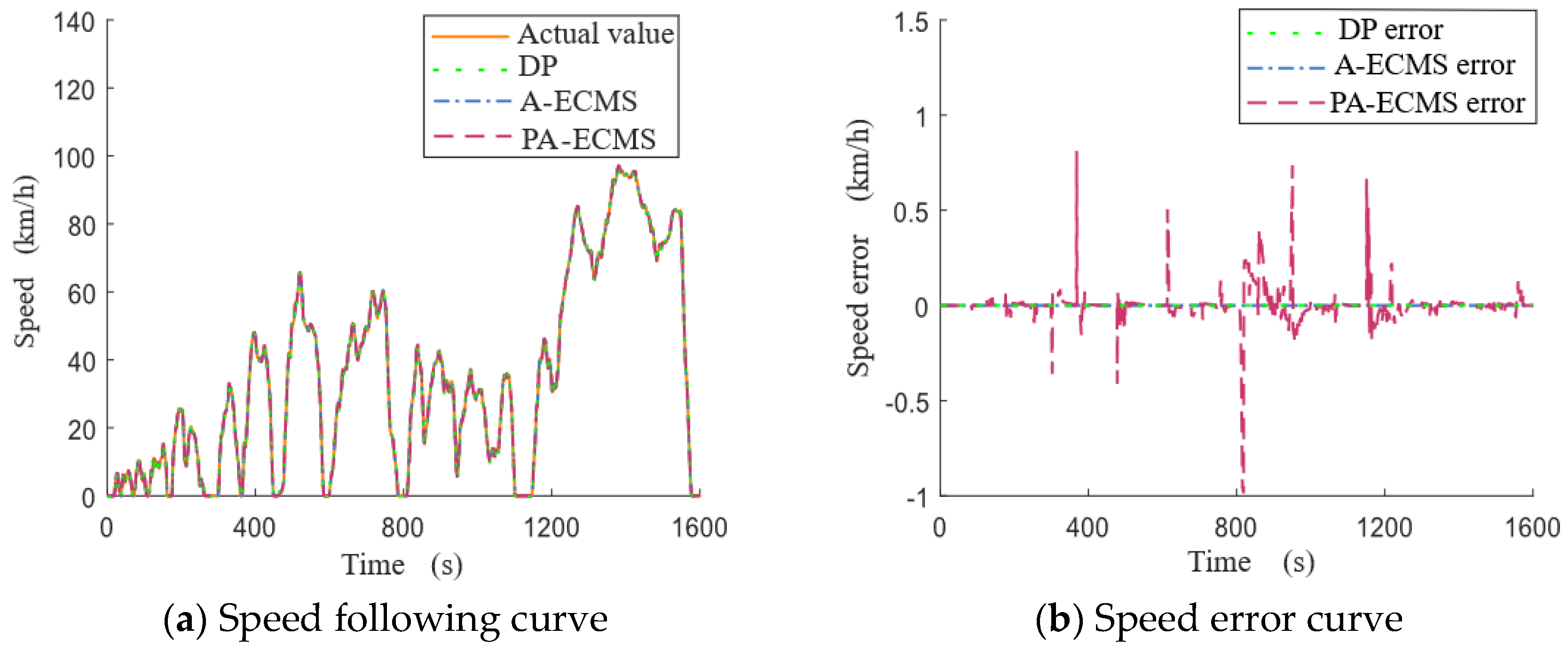
Figure 10 presents the vehicle speed trajectories used in the lower-layer comparison and the corresponding tracking errors. The A-ECMS and PA-ECMS cases follow the prescribed CHTC-LT reference trajectory with acceptable tracking accuracy. For the DP case, the CHTC-LT speed trajectory is prescribed directly rather than optimized by DP; therefore, the DP speed curve is included only to demonstrate that the lower-layer strategies are evaluated under the same driving cycle condition.

Figure 10. Comparison of vehicle speed tracking and speed errors under three strategies.

(2)

Battery SOC Variation

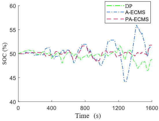
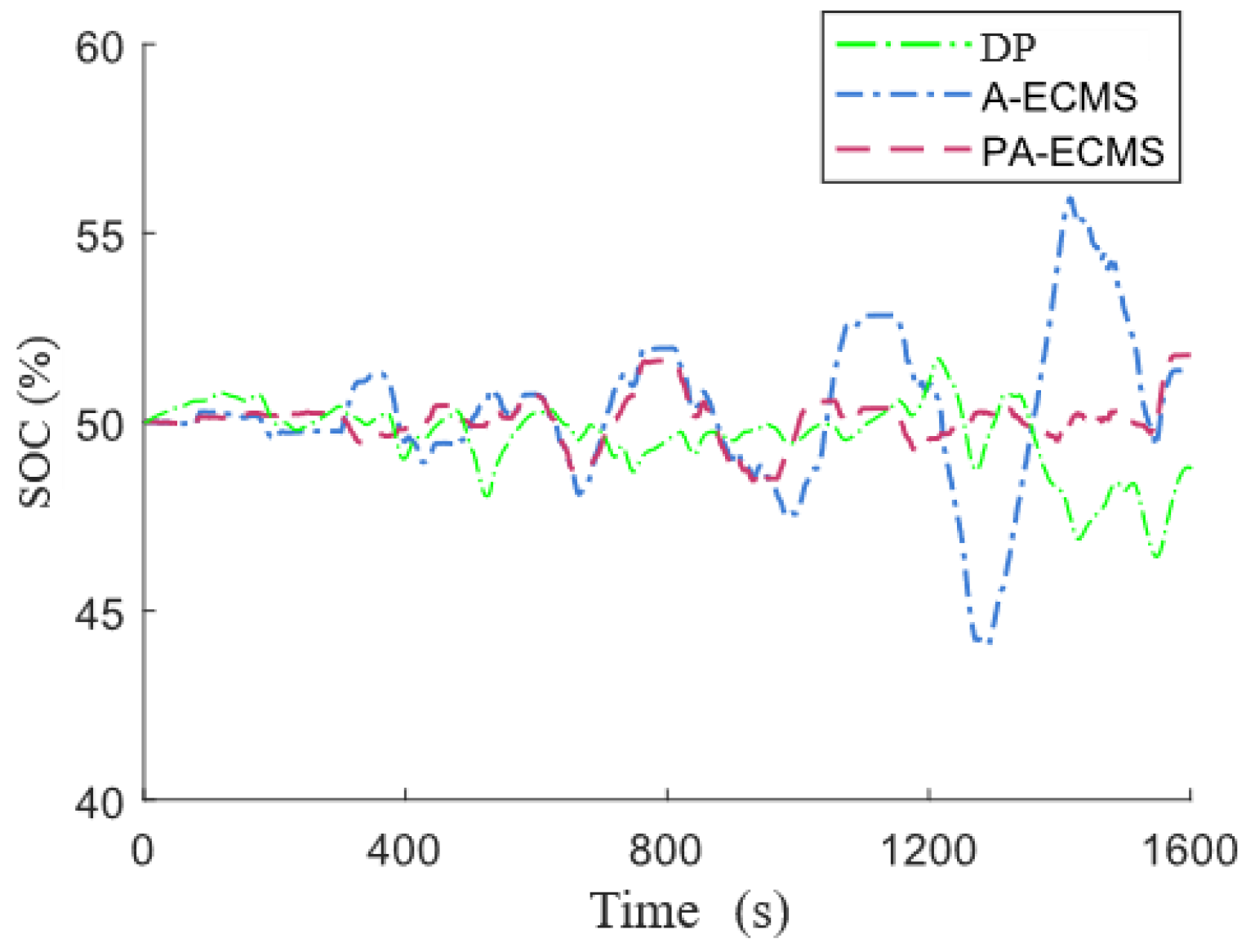
Figure 11 compares the SOC trajectories of A-ECMS, PA-ECMS, and DP. Compared with A-ECMS and DP, PA-ECMS exhibits a smoother SOC trajectory while maintaining the final SOC close to its initial value, indicating improved SOC regulation under the investigated cycle. Nevertheless, this smoother SOC behavior should not be interpreted as evidence of improved battery lifetime, since battery aging, current-rate effects, and temperature effects are not considered in the present model.

Figure 11. Comparison of battery SOC trajectories under three strategies.

(3)

Fuel and Electricity Consumption

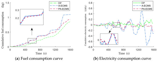
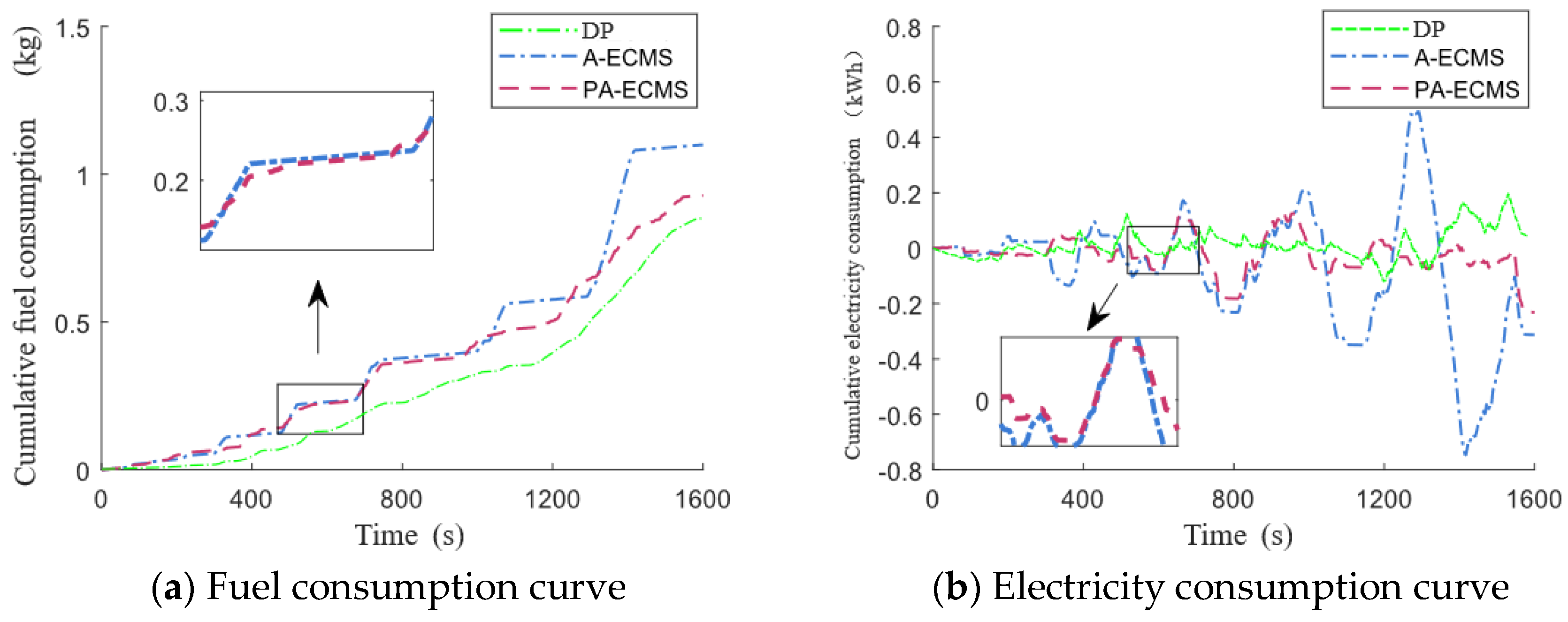
Figure 12 presents the cumulative fuel consumption and electrical energy consumption obtained under the three control strategies. As shown in Figure 12a, the PA-ECMS achieves lower cumulative fuel consumption than the conventional A-ECMS, whereas the DP strategy yields the lowest cumulative fuel consumption among the three strategies. Therefore, the fuel-consumption improvement of PA-ECMS is observed relative to A-ECMS rather than DP. Although the fuel consumption of A-ECMS and PA-ECMS shows a similar increasing trend in the early stage, the PA-ECMS curve demonstrates a more stable growth pattern in the later phase, whereas the A-ECMS curve exhibits more pronounced fluctuations. This indicates that the proposed PA-ECMS method provides improved stability in energy management and better fuel economy performance.

Figure 12. Comparison of cumulative fuel and electricity consumption under three strategies.

As seen in Figure 12b, the three strategies exhibit different battery energy trajectories and net battery energy changes, which are also reflected in their different terminal SOC values. These differences result from the combined effects of power allocation, battery charging, and motor energy consumption over the driving cycle. Therefore, the signed battery energy consumption should not be interpreted as a direct measure of regenerative braking efficiency. Fuel consumption and battery energy change are instead considered jointly through the comprehensive operating cost when evaluating the overall economic performance.

To more intuitively evaluate the advantages of the PA-ECMS, Table 7 presents the key operational performance indicators of the DP, A-ECMS, and PA-ECMS strategies obtained from simulation. The results show that PA-ECMS outperforms the conventional A-ECMS in fuel economy while exhibiting smoother SOC variation under the investigated cycle. Specifically, the fuel consumption of PA-ECMS is 0.9286 kg, which is reduced by 15.6%, compared with 1.0997 kg for A-ECMS. Meanwhile, its final SOC is maintained at 51.77%, and the electricity consumption is −0.2316 kWh, indicating that the proposed strategy can achieve a more balanced energy distribution while ensuring stable battery SOC.

Table 7. Simulation results of three strategies under the CHTC-LT cycle conditions.

Strategy	DP	A-ECMS	PA-ECMS
Final SOC (%)	48.96	51.37	51.77
Accumulated fuel consumption (kg)	0.8593	1.0997	0.9286
Net battery electricity consumption (kWh)	0.0394	−0.3129	−0.2316
Comprehensive cost (RMB)	8.1109	10.0712	8.5320

Note: Positive values indicate net battery-energy consumption, whereas negative values indicate net battery charging.

The raw fuel consumption results show that PA-ECMS consumes 0.9286 kg of fuel, representing a reduction of approximately 15.6% relative to A-ECMS (1.0997 kg). However, its fuel consumption is approximately 8.1% higher than that of DP (0.8593 kg), and DP therefore remains the lowest fuel consumption strategy among the three cases. Because the final SOC values are not identical, these raw fuel consumption values are not used alone to determine the overall economic ranking. Instead, the comprehensive operating cost defined above is used to account jointly for fuel consumption and the signed net battery electricity consumption.

To further evaluate the economic performance of different strategies, the comprehensive operating cost is calculated based on a fuel price of RMB 9.4/kg (approximately USD 1.30/kg) and an electricity price of RMB 0.85/kWh (approximately USD 0.12/kWh). To further evaluate the economic performance of the three strategies in practical operation, the comprehensive operating cost is calculated as:

$$C=9.4Q_f+0.85Q_e$$

(34)

In the equation, C represents the comprehensive cost in yuan; $Q_f$ denotes the cumulative fuel consumption in kilograms; and $Q_e$ denotes the signed net battery electricity consumption in kilowatt-hours, where positive values increase the operating cost and negative values are treated as an electricity credit, allowing fuel consumption and terminal battery energy differences to be evaluated within a unified cost framework.

The results indicate that the comprehensive cost of PA-ECMS is RMB 8.5320, which is 15.3% lower than that of A-ECMS (RMB 10.0712). Compared with the DP strategy (RMB 8.1109), it is only 5.2% higher. These results demonstrate that the PSO-calibrated PA-ECMS improves lower-layer power allocation and economic performance relative to the conventional A-ECMS under the investigated CHTC-LT cycle.

4.4. Validation of the Energy Management Strategy Considering Road Gradient

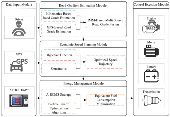
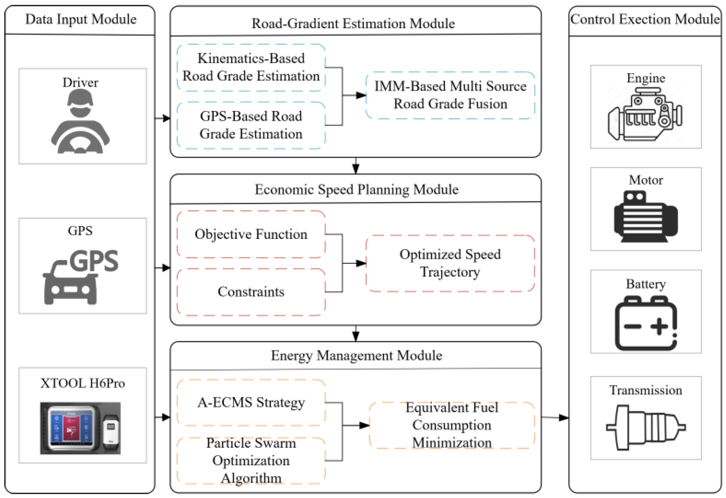
To evaluate the complete hierarchical control framework under real road conditions, a MATLAB/Simulink-based simulation platform is established, as shown in Figure 13. The primary integrated comparison is conducted between the conventional PID + A-ECMS framework and the proposed MPC + PA-ECMS framework. The DP result is retained as an offline lower-layer power split reference for additional performance comparison. Since the present DP implementation follows a prescribed vehicle speed trajectory and does not perform upper-layer speed planning, it is not treated as a directly matched integrated benchmark.

Figure 13. Simulation platform. Note: The IMM-KF estimates the current road gradient, whereas the future gradient sequence required by the MPC is extracted from a pre-reconstructed route-gradient profile. Arrows indicate information and signal flow, while the blue, red, and orange dashed boxes distinguish the functional units of the road-gradient estimation, economic speed-planning, and energy management modules, respectively.

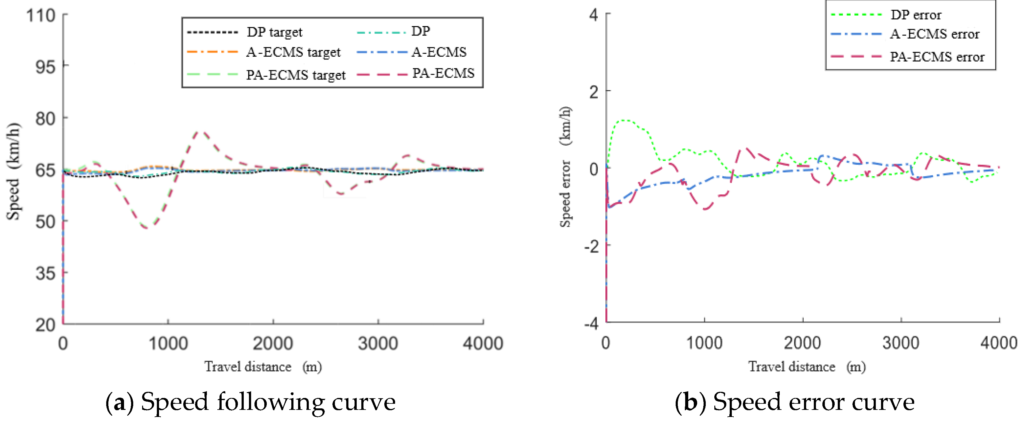
From Figure 14, it can be observed that all three strategies maintain acceptable tracking of the prescribed speed profile, and the corresponding speed errors remain within approximately ±2 km/h during the tested cycle. Therefore, the different energy management strategies exhibit comparable speed tracking performance. The main difference among these strategies lies in their energy management behaviors. In the proposed hierarchical framework, the IMM-KF provides an estimate of the current road gradient, whereas the upper-layer MPC obtains the future gradient sequence over its prediction horizon from the pre-reconstructed route-gradient profile.

Figure 14. Comparison results of three strategies under actual road conditions.

In the present comparison, the benchmark and DP cases do not include the gradient-aware upper-layer speed-planning function of the proposed framework. However, their roles are different: A-ECMS represents the conventional online lower-layer energy management strategy, whereas DP serves as an offline reference for lower-layer power split optimization. On uphill segments, the engine operates at high load for extended periods to maintain the cruising speed, resulting in increased fuel consumption. On downhill segments, due to the lack of effective control over deceleration and energy recovery processes, part of the braking energy cannot be fully utilized, leading to reduced energy recovery efficiency.

To more intuitively evaluate the performance of the proposed strategy, Table 8 compares the key operational indicators of DP, PID + A-ECMS, and MPC + PA-ECMS. The proposed MPC + PA-ECMS framework achieves a total fuel consumption of 0.4613 kg, representing a reduction of approximately 4.0% compared with 0.4803 kg for PID + A-ECMS.

Table 8. Simulation comparison results of three strategies under actual road conditions.

Strategy	Total Fuel Consumption (kg)	Total Electricity Consumption (kWh)	Final SOC (%)	Cost (RMB)
DP	0.4212	0.0103	49.53	3.9680
PID + A-ECMS	0.4803	0.0189	49.76	4.5309
MPC + PA-ECMS	0.4613	−0.0238	50.17	4.3160

Note: The DP strategy is an offline lower-layer power-split benchmark evaluated under a prescribed vehicle speed trajectory and does not include the upper-layer speed-planning function; therefore, it should not be regarded as a fully equivalent integrated strategy to PID + A-ECMS or MPC + PA-ECMS.

In terms of state of charge (SOC), the final SOC of the proposed strategy is 50.17%, compared with 49.53% for DP and 49.76% for PID + A-ECMS. Thus, the proposed strategy maintains the terminal SOC closer to its initial value of 50% under the investigated real-road simulation.

Regarding battery energy usage, DP and PID + A-ECMS exhibit positive net electricity consumption of 0.0103 and 0.0189 kWh, respectively, whereas MPC + PA-ECMS exhibits a net value of −0.0238 kWh, indicating a small net battery-energy gain over the evaluated route. Because the terminal SOC values differ among the strategies, fuel consumption and battery-energy change are considered jointly through the comprehensive operating cost. The comprehensive cost of MPC + PA-ECMS is RMB 4.3160, which is approximately 4.7% lower than that of PID + A-ECMS (RMB 4.5309), although it remains higher than that of the offline DP reference (RMB 3.9680). Overall, compared with PID + A-ECMS, the proposed framework reduces both fuel consumption and comprehensive operating cost while maintaining the terminal SOC close to its initial value.

The improvement levels in the CHTC-LT and real-road cases are not directly comparable because they are obtained from different comparisons. The 15.3% reduction in Section 4.3 reflects the lower-layer PA-ECMS improvement under a fixed CHTC-LT speed profile, whereas the 4.7% reduction in Section 4.4 reflects the complete MPC + PA-ECMS framework under real-road conditions. The smaller real-road improvement is mainly associated with more variable grade-induced power demand and constraints, while the larger CHTC-LT benefit may also include cycle-specific PSO calibration effects.

The two control layers contribute through different mechanisms: the upper-layer MPC reduces vehicle-level energy demand through economic speed planning, whereas the lower-layer PA-ECMS improves engine–motor power allocation. Therefore, the improvement of the complete framework results from their coordinated effects rather than from a single control block.

5. Conclusions

This study proposes an energy management strategy for a hybrid commercial vehicle considering road gradient, and the main conclusions can be summarized as follows:

(1)

An IMM-KF-based road gradient estimation module is established and validated under constant and variable gradient conditions to improve current road gradient perception.

(2)

The MPC-based speed-planning strategy reduces vehicle level energy demand by optimizing the vehicle speed trajectory using route gradient preview information.

(3)

The PSO-based adaptive energy management strategy enhances power distribution between the engine and motor while maintaining battery SOC stability.

(4)

Comparative simulations show that the proposed method reduces fuel consumption and comprehensive operating cost relative to the conventional A-ECMS, while the offline DP strategy retains the lowest fuel consumption and operating cost. The proposed method therefore demonstrates improved economic performance and simulation-based computational feasibility within the present MATLAB/Simulink framework. However, embedded real-time feasibility has not been demonstrated because controller execution time, solver timing, processor information, and hardware-in-the-loop performance have not been evaluated.

Although the present study has achieved the above contributions, it also has the following limitations.

(1)

The road gradient estimation module is validated using real road measurement data, whereas the upper-layer speed-planning, lower-layer energy management, and integrated hierarchical control strategies are evaluated through MATLAB/Simulink simulations under simplified vehicle dynamics and idealized assumptions.

(2)

The current framework focuses on road gradient effects and does not explicitly consider traffic flow or driver behavior. In congested conditions, traffic-dominated speed profiles and frequent stop-and-go operation may reduce the benefit of grade-based speed planning and increase power-demand fluctuations, potentially affecting fuel economy and SOC regulation. These effects have not been quantitatively evaluated in the present study.

(3)

Future work will be carried out based on the current data-driven simulation framework. Hardware-in-the-loop (HIL) experiments and real-vehicle road tests will be conducted to evaluate controller execution time, solver performance, communication delay, and embedded real-time feasibility, and to further verify the robustness of the proposed method in real vehicle systems.

References

- Zeng, X.; Qian, Q.; Song, D.; Gu, J.; Yuan, W. Slope estimation algorithm and its implementation based on acceleration correction. Qiche Gongcheng/Automot. Eng. 2020, 42, 1369–1377. [Google Scholar] [CrossRef]
- Mutta, S.; Subramanian, S.C.; Gunti, S.; Shankar, V.; Parag, D. Model based road slope and mass estimation of road vehicles. In Proceedings of the 2021 IEEE Transportation Electrification Conference (ITEC-India), Gurugram, India, 16–19 December 2021; pp. 1–6. [Google Scholar] [CrossRef] [Scilit]
- Feng, Z.; Du, W.; Chng, C.-B.; Chui, C.-K.; Zhao, S. Meta-learning-based predictive energy management for 4WD battery electric vehicles. IEEE Trans. Veh. Technol. 2024, 73, 6395–6408. [Google Scholar] [CrossRef] [Scilit]
- Li, E.; He, W.; Yu, H.; Xi, J. Model-based embedded road grade estimation using quaternion unscented kalman filter. IEEE Trans. Veh. Technol. 2022, 71, 3704–3714. [Google Scholar] [CrossRef] [Scilit]
- Zhu, Z.; He, C.; Li, J.; Liu, X.; Ma, R. The prediction model for road slope of electric vehicles based on stacking framework of deep learning. IEEE Access 2023, 11, 22880–22888. [Google Scholar] [CrossRef] [Scilit]
- Tian, D.; Jin, L.; Zhang, Z.; Li, H. Vehicle state estimation based on multidimensional information fusion. IEEE Access 2022, 10, 76220–76232. [Google Scholar] [CrossRef] [Scilit]
- Jia, C.; Zhou, J.; He, H.; Li, J.; Wei, Z.; Li, K. Health-conscious deep reinforcement learning energy management for fuel cell buses integrating environmental and look-ahead road information. Energy 2024, 290, 130146. [Google Scholar] [CrossRef] [Scilit]
- Linfeng, Z.; Manling, Z.; Bixin, C.; Yuan, Q.; Jinfang, H. One estimation method of road slope and vehicle distance. Measurement 2023, 208, 112481. [Google Scholar] [CrossRef] [Scilit]
- Guo, J.; He, C.; Li, J.; Wei, H. Slope estimation method of electric vehicles based on improved sage–husa adaptive kalman filter. Energies 2022, 15, 4126. [Google Scholar] [CrossRef] [Scilit]
- Huang, Z.; Fan, X.; Yu, X.; Wang, L. Joint estimation method of vehicle mass and road slope based on unscented kalman filter. Sens. Rev. 2025, 45, 625–635. [Google Scholar] [CrossRef] [Scilit]
- Liu, Y.; Wei, L.; Fan, Z.; Wang, X.; Li, L. Road slope estimation based on acceleration adaptive interactive multiple model algorithm for commercial vehicles. Mech. Syst. Signal Process 2023, 184, 109733. [Google Scholar] [CrossRef] [Scilit]
- Ma, M.; Hu, J.; Xiao, R. Energy management strategy with model prediction for fuel cell hybrid trucks considering vehicle mass and road slope. Energy Convers. Manag. 2025, 333, 119791. [Google Scholar] [CrossRef] [Scilit]
- Qin, D.; Wang, K.; Feng, J.; Liu, Y.; Cheng, K.; Xia, Y. Road slope estimation based on unscented kalman filtering and gated recurrent unit. Qiche Gongcheng/Automot. Eng. 2022, 44, 1547–1555+1580. [Google Scholar] [CrossRef]
- Gao, L.; Wu, Q.; He, Y. Road slope estimation for heavy-duty vehicles under the influence of multiple source factors in real complex road environments. Mech. Syst. Signal Process 2024, 208, 110973. [Google Scholar] [CrossRef] [Scilit]
- Liu, Z.; Cheng, S.; Liu, J.; Wu, Q.; Li, L.; Liang, H. A novel braking control strategy for hybrid electric buses based on vehicle mass and road slope estimation. Chin. J. Mech. Eng. 2022, 35, 150. [Google Scholar] [CrossRef] [Scilit]
- Yue, F.; Liu, Q.; Kong, Y.; Zhang, J.; Xu, N. A predictive energy management strategy for multi-energy source vehicles based on full-factor trip information. Sensors 2022, 22, 23. [Google Scholar] [CrossRef] [Scilit]
- Tao, F.; Fu, Z.; Gong, H.; Ji, B.; Zhou, Y. Twin delayed deep deterministic policy gradient based energy management strategy for fuel cell/battery/ultracapacitor hybrid electric vehicles considering predicted terrain information. Energy 2023, 283, 129173. [Google Scholar] [CrossRef] [Scilit]
- Chai, H.; Zhao, X.; Yu, Q.; Wang, S.; Han, Q.; Zheng, Z. Adaptive equivalent consumption minimization strategy based on road grade estimation for a plug-in hybrid electric truck. J. Energy Storage 2023, 70, 108035. [Google Scholar] [CrossRef] [Scilit]
- Zhang, Y.; You, X.; Song, Y.; Zhao, Y.; Wei, Z.; Jiao, X. Hierarchical eco-driving of connected hybrid electric vehicles: Integrating predictive cruise control and cost-to-go approximation-guided energy management. Energy 2025, 319, 134579. [Google Scholar] [CrossRef] [Scilit]
- Wang, Y.; Li, X.; Zhang, P.; Zheng, X. Real-time optimization algorithm for truck predictive cruise based on ADAS map. Qiche Gongcheng/Automot. Eng. 2020, 42, 1335–1339+1411. [Google Scholar] [CrossRef]
- Qu, L.; Zhuang, W.; Chen, N. Instantaneous velocity optimization strategy of electric vehicle considering varying road slopes. In Proceedings of the 2019 Chinese Control and Decision Conference (CCDC), Nanchang, China, 3–5 June 2019; pp. 5483–5488. [Google Scholar] [CrossRef] [Scilit]
- Ju, F.; Zhuang, W.-C.; Wang, L.-M.; Liu, J.-X.; Wang, Q. Velocity planning strategy for economic cruise of hybrid electric vehicles. Zhejiang Daxue Xuebao (Gongxue Ban)/J. Zhejiang Univ. (Eng. Sci.) 2021, 55, 1538–1547. [Google Scholar] [CrossRef]
- Polverino, P.; Adinolfi, E.A.; Pianese, C. Target speed computation through predictive cruise control for vehicles energy consumption reduction. Energy Convers. Manag. 2023, 298, 117757. [Google Scholar] [CrossRef] [Scilit]
- Wang, F.; Hong, Y.; Zhao, X. Research and comparative analysis of energy management strategies for hybrid electric vehicles: A review. Energies 2025, 18, 2873. [Google Scholar] [CrossRef] [Scilit]
- Li, Y.; He, H.; Khajepour, A.; Wang, H.; Peng, J. Energy management for a power-split hybrid electric bus via deep reinforcement learning with terrain information. Appl. Energy 2019, 255, 113762. [Google Scholar] [CrossRef] [Scilit]
- Shi, D.; Rong, X.; Wang, S.; Chen, L. Fuzzy adaptive equivalent consumption minimization strategy for hybrid electric vehicle based on power ratio. Hsi-Chiao Tung Ta Hsueh/J. Xi’an Jiaotong Univ. 2022, 56, 12–21. [Google Scholar] [CrossRef]
- Liu, X.; Qin, D.; Wang, S. Minimum energy management strategy of equivalent fuel consumption of hybrid electric vehicle based on improved global optimization equivalent factor. Energies 2019, 12, 2076. [Google Scholar] [CrossRef] [Scilit]
- Zhou, L.; Yang, D.; Zeng, X.; Zhang, X.; Song, D. Multi-objective real-time energy management for series–parallel hybrid electric vehicles considering battery life. Energy Convers. Manag. 2023, 290, 117234. [Google Scholar] [CrossRef] [Scilit]
- Gomozov, O.; Trovao, J.P.F.; Kestelyn, X.; Dubois, M.R. Adaptive energy management system based on a real-time model predictive control with nonuniform sampling time for multiple energy storage electric vehicle. IEEE Trans. Veh. Technol. 2017, 66, 5520–5530. [Google Scholar] [CrossRef] [Scilit]
- Boukoberine, M.N.; Zia, M.F.; Berghout, T.; Benbouzid, M. Reinforcement learning-based energy management for hybrid electric vehicles: A comprehensive up-to-date review on methods, challenges, and research gaps. Energy AI 2025, 21, 100514. [Google Scholar] [CrossRef] [Scilit]
- Li, Z.; Long, W.; Tian, H. Current applications and future prospects of deep reinforcement learning in energy management for hybrid power systems. Energies 2026, 19, 2216. [Google Scholar] [CrossRef] [Scilit]
- Tota, A.; Galvagno, E.; Dimauro, L.; Vigliani, A.; Velardocchia, M. Energy management strategy for hybrid multimode powertrains: Influence of inertial properties and road inclination. Appl. Sci. 2021, 11, 11752. [Google Scholar] [CrossRef] [Scilit]
- He, H.; Guo, J.; Sun, C. Road grade prediction for predictive energy management in hybrid electric vehicles. Energy Procedia 2017, 105, 2438–2444. [Google Scholar] [CrossRef] [Scilit]
- Ciravegna, L.; Dimauro, L.; Frison, G.; Alberti, F.; Galvagno, E.; Sorniotti, A. Energy-efficient eco-driving for human-driven electric vehicles via adaptive drivability maps with predictive driver modeling. Appl. Energy 2026, 420, 128077. [Google Scholar] [CrossRef] [Scilit]
- Zhang, P.; Wu, X.; Du, C.; Xu, H.; Wang, H. Adaptive equivalent consumption minimization strategy for hybrid heavy-duty truck based on driving condition recognition and parameter optimization. Energies 2020, 13, 5407. [Google Scholar] [CrossRef] [Scilit]
Disclaimer/Publisher’s Note: The statements, opinions and data contained in all publications are solely those of the individual author(s) and contributor(s) and not of MDPI and/or the editor(s). MDPI and/or the editor(s) disclaim responsibility for any injury to people or property resulting from any ideas, methods, instructions or products referred to in the content. |
© 2026 by the authors. Licensee MDPI, Basel, Switzerland. This article is an open access article distributed under the terms and conditions of the Creative Commons Attribution (CC BY) license.