


Abstract
This study examines the agricultural energy transition in 25 European Union Member States over 2005–2024, focusing on energy intensity, fossil-fuel dependence, and carbon intensity. It integrates multi-regional Kaya–LMDI decomposition, Tapio decoupling analysis, and σ- and conditional β-convergence models to identify the components associated with changes in direct energy-related agricultural CO2 emissions, assess their relationship with real agricultural gross value added, and determine whether national performance gaps are narrowing. The results show that declining energy intensity and fossil dependence were the main emissions-reducing components, while changes in country structure and carbon intensity partly offset these gains. Within the EU-25 analytical sample, the baseline comparison indicates a shift from recessive decoupling before 2020 to strong decoupling over 2020–2024. Sensitivity tests confirm the robustness of post-2020 strong decoupling, although the characterization of the pre-2020 period is sensitive to sample composition. Conditional β-convergence is observed for all three indicators, whereas σ-convergence is found only for energy intensity; fossil dependence and carbon intensity continue to exhibit substantial cross-country dispersion. Bias-corrected estimates preserve the direction of conditional catch-up but indicate slower adjustment, particularly for fossil dependence. The study’s novelty lies in jointly evaluating emissions decomposition, decoupling, and distributional change while distinguishing relative catch-up towards country-specific trajectories from convergence towards a common EU level. The findings identify energy efficiency, fossil-energy substitution, and differentiated national conditions as relevant areas for CAP-related monitoring and policy consideration. The conclusions concern specifically the energy-related component of agricultural decarbonization.
1. Introduction
The agricultural sector is increasingly relevant to the European Union’s energy transition. Although agriculture accounts for a relatively small share of final energy consumption, energy availability and prices substantially affect production costs, farm income, and resilience. Energy is directly required for machinery, transport, irrigation, drying, cooling, storage, and greenhouse operation. Agriculture also indirectly consumes energy embodied in fertilizers, pesticides, machinery, and other manufactured inputs. Consequently, the food system can be viewed as a complex energy chain with important implications for greenhouse gas emissions and climate change [1,2].
Improving agricultural energy performance requires a combination of energy-efficiency measures, renewable-energy adoption, fossil-fuel substitution, and investment in more resilient production systems. Available technological options include precision farming, drones, tractor-mounted equipment, efficient irrigation, electrification, and the production of alternative fuels from agricultural and organic waste. However, their adoption depends on financial viability, grid access, stable legislation, administrative capacity, and effective advisory services [3].
A clear definition of the emissions boundary is essential when assessing the environmental consequences of agricultural energy use. Carbon accounting depends on the activities included, data quality, and the application of appropriate emission factors [1,2,3,4]. The present study focuses exclusively on direct energy-related CO2 emissions from agricultural fuel consumption. It therefore does not provide a complete assessment of agriculture’s climate impact, which would also include methane and nitrous oxide emissions from livestock, agricultural soils, manure management, and land-use change.
The Common Agricultural Policy provides the main institutional framework for supporting the agricultural energy transition. The CAP Strategic Plans allow Member States to design interventions that address their specific agricultural, environmental, and socioeconomic conditions [5,6,7,8,9,10]. The indicators developed for the 2023–2027 programming period also provide a basis for monitoring differences among national agricultural systems [7,8,9,10]. Such differentiation is important because the effects of energy prices, input costs, infrastructure, climate, and technological capacity vary considerably across Member States.
This study combines three complementary analytical approaches. First, index decomposition analysis identifies the factors driving changes in energy use and emissions. The logarithmic mean Divisia index within the Kaya framework has been widely applied to the decomposition of energy consumption and greenhouse gas emissions [11,12,13,14,15]. Applications to agriculture include the studies of Robaina-Alves and Moutinho [16], Li et al. [17], Andrei et al. [18], and Peng et al. [19].
Second, Tapio decoupling analysis evaluates whether changes in agricultural emissions are becoming less closely associated with changes in agricultural production [20]. Although decoupling methods have been applied to agriculture and related environmental outcomes, previous studies have generally examined individual countries, regions, or specific policy instruments [18]. Cross-country evidence on the decoupling of direct energy-related agricultural CO2 emissions remains comparatively limited.
Third, convergence analysis investigates whether EU agricultural systems are becoming more similar in terms of energy intensity, fossil-fuel dependence, and carbon intensity. The joint use of β- and σ-convergence makes it possible to distinguish relative catch-up by initially high-intensity countries from an actual reduction in cross-country dispersion.
The novelty of this study lies in integrating Kaya–LMDI decomposition, Tapio decoupling, and convergence analysis within a single framework for 25 EU Member States over the period 2005–2024. This combination provides a multidimensional assessment of changes in direct energy-related agricultural emissions, their underlying drivers, their relationship with agricultural production, and the distribution of energy and carbon performance across countries.
More specifically, the study addresses four research questions:
H1.
Which factors drive changes in direct energy-related agricultural CO2 emissions?
H2.
How has the relationship between agricultural emissions and agricultural production evolved over time?
H3.
Do Member States converge in terms of energy intensity, fossil-fuel dependence, and carbon intensity?
H4.
Does the observed EU-level progress reflect broad-based improvement or improvements concentrated in specific national agricultural systems?
Scientifically, the study connects decomposition, decoupling, and convergence approaches that are usually applied separately. Practically, it provides evidence relevant to the design and monitoring of CAP intervention, aimed at increasing energy efficiency, reducing fossil-fuel dependence, promoting alternative energy sources, and strengthening the resilience of national agricultural systems.
The remainder of the paper is organized as follows. The next section reviews the relevant literature, followed by the data and methods. The empirical results are then presented and discussed, while the final section summarizes the conclusions and policy implications.
2. Literature Review
2.1. Agricultural Energy Use, Emissions Boundaries, and Mitigation Pathways
Modern Agriculture is an energy intensive system not only for the energy required directly for agricultural crops, livestock and their products (for field work, irrigation, etc., including in storage in refrigeration) but also for the indirect energy embedded in the various inputs bought by farmers such as fertilizers, crop protection products, tractors and other machines for field work and storage facilities (barns, cold stores, and others.). The increased agricultural production over the last decades has been made possible to a large extent by the increased use of fossil energy [1,2,3]. However, the relationship between energy inputs and agricultural production is not always straightforward as very low levels of energy can lead to low levels of production and even to high levels of energy use per unit of production. As long as levels of inputs are increased, production will increase with decreasing increments of production efficiency. Hence, increased energy efficiency does not automatically lead to reduced energy use.
The system boundaries for assessment of energy use and for calculation of greenhouse gas emissions of agriculture can be restricted to the farm or the whole food system. Within the farm system the direct energy use for agricultural production in terms of fuels and electricity is calculated. The whole food system includes processing, distribution, retail, preparation, storage in cold, other storage and waste management. For assessment of the whole food system the energy use is calculated for different stages of the food supply chain for different commodities and for different type of energy. Tang [4] stresses the importance of clear system boundaries for carbon accounting. Besides the direct fuel-combustion CO2-emissions also methane and nitrous oxide emissions from animals, manure, fertilized soils and from land use changes have to be taken into account for agriculture. For agricultural mitigation of climate change, a portfolio of energy, biological, land use and carbon sink options is developed. Sokal and Kachel [21] and Küfeoğlu [22] discuss options for agricultural mitigation of climate change. Source-oriented mitigation of greenhouse gas emissions can be supported by ecosystem services and even carbon sinks can be created by agriculture, as in Li et al. [23].
Energy used in agriculture is not always visible because it is largely used for mechanization of farming. Production of power for tractors and other self-propelled machines and for other machinery used in the field constitutes by far the greatest amount of energy used in agriculture. For many of the different tasks that are carried out in the field, a high amount of power is required for a long period of time. The majority of this energy is produced by burning liquid fuels. There are many different management options that can be used to reduce the energy use for agriculture without having to decrease production levels. Some of the examples are to match the power of tractors and other machines to the implements that are used, to make the best use of the different gears and engine speeds, to keep filters in good working order and to make sure that the correct tire pressure is maintained.
In addition to these examples, minimizing wheel slip, improvement of field traffic and reduction in the number of turns that are made are other ways in which energy use for agriculture can be reduced. Many of these options can be supported by precision agriculture using techniques such as precision guidance, intelligent transmission management, controlled traffic farming and the use of lighter machinery, including autonomous machines. However, the potential for these options will vary depending on a number of factors, including the size of the farm, the knowledge, skills and experience of the farmer and his or her staff, the times of the year when work in the field can be carried out, the field conditions and the age and compatibility of the farmer’s machinery. Agriculture can also be supplied with alternative energy solutions that can be evaluated by a life cycle assessment (LCA). For example, Özer et al. [24] investigated a common-rail tractor engine fueled with a bioalcohol blend containing nanoparticles. The bioalcohol was produced from fig waste and the experiments showed that the used fuel mixture could reduce the share of the fossil fuel in the fuel and also can valorize the fig waste produced. The results of the study need to be evaluated by the assessment of the feedstock supply, the energy required for production, the incompatibility of the fuel with the engine, the storage requirements and costs as well as the life cycle greenhouse gas emissions including the emissions from production. The main thrust of precision agriculture is to increase the efficiency of production and save energy.
At the field level, a number of practices can increase production while reducing the negative impacts of inputs. For example, tillage could be reduced by using precision agriculture to optimize field operations, and by using sensors and precision agriculture to apply exact amounts of fertilizers, pesticides, and seed to specific sections of the field. In addition, the use of digital farm planning, and variable rate applications of seed, fertilizers, and pesticides, could save energy and reduce negative impacts. There are also many examples where drones are used for precision spraying, and where they save a large amount of energy compared with conventional methods of spraying using tractors equipped with sprayers. According to Safaeinejad et al. [25], for example, drone spraying saved 85% of energy and 79% of global warming potential compared with conventional spraying methods. However, drone spraying also has a number of limitations, including very high production costs, battery weight, low flying time and range, lack of trained pilots, and very low scalability [25]. In general, precision agriculture requires a combination of efficient machinery, information, and management.
Another strategy to generate energy from agricultural production is to use it for the generation of solar energy, biogas, biomethane or bioenergy, etc., on the farm. Thereby, the farmers can generate new income possibilities and be supplied with energy in a self-sufficient manner. For the implementation of these strategies, stable incentives, facilitating administrative procedures, access to the grid, funds for investments and appropriate advisory services are needed. A large variety of strategies for the agricultural mitigation of climate change are available. The effectiveness, however, strongly depends on the national and farm-specific framework conditions such as specialization, farm size, age of machinery, fuels used, generation of electricity, energy generating infrastructure on the farm and the institutional framework.
2.2. Decomposition of Energy-Related Emissions and the Role of Country Structure
Decomposition analysis provides an accounting framework for identifying the factors underlying changes in energy use and emissions. The Kaya identity expresses emissions as the product of socioeconomic and energy-system components and can be adapted to the sector and geographical scale under investigation [26,27]. Index decomposition analysis then allocates the observed change in an aggregate indicator among a defined set of activity, structural, intensity, and energy-composition effects. Unlike econometric determinants models, decomposition does not estimate causal parameters; it provides an exact or near-exact attribution of an observed change to the factors embedded in the identity [11,12,14]. Structural decomposition analysis offers an input–output-based alternative for embodied emissions, but IDA is less data-intensive and is readily applied to annual sectoral panels [28].
The logarithmic mean Divisia index has become one of the most widely used IDA methods because it can achieve perfect decomposition and consistency in aggregation. Earlier decomposition procedures often generated an unexplained residual, preventing the full observed change from being assigned to the selected drivers. The development of logarithmic-mean weighting addressed this weakness and established a framework in which subgroup effects add consistently to the aggregate result [29,30,31]. This property is particularly important in multi-country analysis because country contributions must reproduce the regional total.
LMDI can accommodate multiple drivers and can be implemented in additive or multiplicative form. Additive decomposition expresses effects in the physical unit of the dependent variable, making it suitable for identifying the number of tonnes of CO2 added or avoided by each factor. Multiplicative decomposition expresses effects as ratios and facilitates relative interpretation. Ang et al. [32] discuss the relationships among decomposition approaches, while Ang [11,12] provides guidance on factor design, logarithmic-mean weights, zero-value treatment, and implementation. LMDI also supports fixed-base and chained analyses. Fixed-base results summarize the cumulative change between two endpoints, whereas annual chained effects reveal how drivers change during crises, recoveries, and policy periods. This temporal flexibility has made LMDI useful for energy-efficiency accounting and policy evaluation [33,34].
Cross-country applications require a spatial or multi-regional extension because aggregate emissions can change even when total activity is stable if the geographical distribution of production changes. Zhang and Ang [35] emphasize comparability and structural definition in cross-country decomposition, and Lee and Oh [36] demonstrate that logarithmic-mean methods can support both time-series and cross-sectional comparisons. Fernández González et al. [34] use a multilevel LMDI approach to separate inter-country and within-group changes in EU energy consumption, illustrating the policy value of distinguishing aggregate activity from regional structure.
For an integrated agricultural area, aggregate direct energy-related emissions can be represented as:
where Y is aggregate real agricultural GVA, Si is country i’s share of aggregate GVA, EIi is energy use per unit of real GVA, FSi is the fossil share of selected energy use, and CIi is CO2 emissions per unit of fossil energy. The corresponding additive decomposition is:
Ct = Σi Yt × Sit × EIit × FSit × CIit
ΔC = ΔC(Activity) + ΔC(Structure) + ΔC(Energy intensity) + ΔC(Fossil share) + ΔC(Carbon intensity)
The activity effect measures the emissions consequence of aggregate expansion or contraction in real agricultural GVA. The country-structure effect captures changes in the geographical distribution of agricultural activity. It is positive when activity shifts towards countries with relatively high combined energy intensity, fossil dependence, and carbon intensity, and negative when activity shifts towards countries with cleaner profiles. This term does not measure embodied emissions in intra-EU trade and does not imply that production relocation is intrinsically undesirable. Rather, it identifies how the spatial allocation of directly measured production influences the aggregate outcome.
Country structure is particularly relevant in the integrated EU agricultural market. Member States operate within common market and CAP frameworks but differ in climate, irrigation requirements, greenhouse production, crop and livestock specialization, farm scale, machinery age, energy infrastructure, and fuel mixes. Changes in productivity, prices, investment, comparative advantage, and demand can alter each country’s share of aggregate agricultural GVA. A shift towards countries with more energy- or carbon-intensive production profiles can raise EU-wide emissions even if total agricultural activity remains unchanged, whereas a shift towards cleaner systems can reduce them. The structural effect therefore connects market integration with the geographical dimension of the energy transition [37].
The remaining factors distinguish three mechanisms that are often conflated. The energy-intensity effect reflects changes in energy required per unit of real agricultural value and is influenced by technology, machinery, farm organization, irrigation, heating, and output composition. The fossil-share effect isolates changes caused by electrification, renewable energy, bioenergy, or other forms of fuel substitution. The carbon-intensity effect captures emissions per unit of fossil energy and may reflect changes in fossil-fuel composition, emission factors, fuel quality, combustion conditions, and equipment performance. Separating these terms is important because fossil dependence can decline while the remaining fossil mix becomes more carbon intensive, or carbon intensity can improve without a substantial reduction in the fossil share.
Agricultural applications confirm the usefulness of this distinction. Robaina-Alves and Moutinho [16] decomposed energy-related agricultural GHG emissions in European countries and identified heterogeneous national drivers. Li et al. [17] combined decomposition and environmental-efficiency analysis for 18 EU countries and found energy-intensity improvement to be a major mitigation opportunity. Peng et al. [19] likewise distinguish agricultural structure, energy intensity, fossil dependence, and the carbon factor of fossil energy. The present study builds on this literature through a five-factor multi-regional model covering 25 Member States and by linking the decomposition results to decoupling and convergence analysis.
2.3. Decoupling of Agricultural Output and Emissions
Decoupling analysis evaluates whether economic activity can expand without generating a proportional increase in environmental pressure. Relative decoupling occurs when emissions increase more slowly than output, while absolute or strong decoupling occurs when output increases and emissions decline. Tapio’s [20] elasticity framework combines the relative rates and directions of change to distinguish strong and weak decoupling, coupling, recessive decoupling, and different forms of negative decoupling. The method offers an intuitive classification without imposing a predetermined econometric relationship between environmental pressure and economic activity.
Tapio analysis complements rather than competes with LMDI. Decomposition attributes emissions change to activity, structure, energy intensity, fossil share, and carbon intensity, whereas Tapio classifies the resulting relationship between emissions and agricultural activity. LMDI therefore explains why emissions changed, while Tapio indicates whether the final outcome is compatible with economic expansion or contraction. Identical decoupling states can arise from different mechanisms: strong decoupling may result from efficiency gains, fuel substitution, cleaner combustion, or structural change, while weak or negative decoupling may persist if activity grows rapidly or shifts towards more energy-intensive systems despite technical improvement [12,14].
European studies demonstrate substantial heterogeneity in agricultural emissions trajectories. Robaina-Alves and Moutinho [16] and Li et al. [17] identify major cross-country differences in the drivers and mitigation potential of agricultural energy-related emissions. Peng et al. [19] similarly shows that structural shifts and energy-system characteristics influence agricultural GHG-emission intensity. Direct decoupling evidence is more limited. Andrei et al. [18] apply the Tapio framework to CO2, CH4, and N2O emissions and agricultural output in EU countries and find that classifications vary across countries and time horizons. Memo [38] identifies multiple long-run pathways in Central and Eastern European transition economies, including growth with declining emissions, joint growth of output and emissions, and simultaneous contraction.
Research both within and outside Europe supports the complementary use of decomposition and decoupling approaches. Xie et al. [39] jointly apply LMDI and Tapio analysis to distinguish observed decoupling patterns from their underlying emissions drivers, while Xu and Shi [40] similarly combine decomposition and decoupling to link changes in emissions–activity relationships to their structural determinants. Chun et al. [41] apply both approaches to multi-sector CO2 emissions, further demonstrating their usefulness for interpreting decoupling patterns alongside underlying drivers. Evidence from outside Europe further reinforces this complementarity. Han et al. [42] relate heterogeneous provincial decoupling patterns in China to differences in their underlying drivers; Jiang et al. [43] combine decoupling classification with scenario analysis; Jia et al. [44] integrate LMDI and Tapio methods in the analysis of agricultural emissions and carbon sinks; and Meng et al. [45] associate agricultural decoupling with technology, investment, employment, and emissions intensity. Collectively, these studies show that decomposition and decoupling provide related but distinct information and that their findings are sensitive to geographical scale, emissions boundaries, activity measures, and the period examined.
However, these studies largely integrate decomposition and decoupling without examining whether the resulting transition patterns are accompanied by cross-country convergence. The present study extends this literature by jointly applying multi-regional Kaya–LMDI decomposition, Tapio decoupling, and σ- and conditional β-convergence to EU-25 agriculture, thereby linking aggregate emissions drivers, decoupling dynamics, and the evolution of cross-country heterogeneity within a single analytical framework.
2.4. Convergence in Energy and Environmental Performance
This paper examines whether countries converge over time. From a cross-country perspective, sigma (σ) convergence occurs when differences among countries decline, as reflected in a reduction in cross-sectional dispersion. Beta (β) convergence occurs when countries with initially higher values of a sustainable-energy indicator experience faster subsequent improvement than countries with lower initial values. However, this does not necessarily imply convergence towards a common long-run equilibrium. Countries may instead approach different steady states, as recognized by conditional β-convergence. This concept accounts for persistent differences in technology, production structures, natural resources, institutions, and national energy systems [46,47].
Beta convergence does not necessarily lead to sigma convergence. Statistically significant catch-up may coexist with stable or increasing cross-country dispersion because of changes in country rankings, asymmetric shocks, or differences in national adjustment paths. Thus, although β-convergence is generally necessary for σ-convergence, it is not sufficient to demonstrate that the overall distribution is narrowing [48].
Energy convergence has been examined across different periods, sectors, and country groups. In manufacturing, less energy-productive countries often improve more rapidly, although transition paths differ across countries and sectors. De Groot and Mulder [49] identify both convergence and divergence in electricity and industrial energy productivity, suggesting that countries may move towards different steady states. Liddle [50] finds convergence in electricity intensity among IEA/OECD countries but not in overall energy intensity, with substantial sectoral differences. At the global level, Liddle [51] identifies regional groups converging at different rates. Parker and Liddle [52] similarly find several convergence clubs rather than a single transition path towards cleaner energy systems.
European evidence also indicates persistent heterogeneity. Energy-intensity disparities among the EU-25 declined during the early part of 2003–2014, but convergence subsequently slowed as spatial effects and country re-ranking became more important [53]. Carbon-emissions convergence is more likely among integrated economies at similar stages of development than across highly heterogeneous countries. Common regulation, market integration, technology diffusion, and the exchange of best practices may promote convergence, while differences in economic structures and energy systems may preserve national disparities [54].
Although convergence has been examined for several agricultural indicators, evidence concerning direct energy-related agricultural emissions remains limited. This study therefore analyses three indicators separately: energy intensity, fossil-energy share, and carbon intensity. Convergence in energy intensity does not necessarily imply convergence in the energy mix or in emissions per unit of fossil energy. Accordingly, both σ-convergence and conditional β-convergence are assessed for each indicator.
2.5. CAP, the Agricultural Energy Transition, and Resilience
The CAP 2023–2027 provides the principal policy setting for the agricultural energy transition in the EU. Regulation (EU) 2021/2115 establishes common economic, environmental, and social objectives but delegates the selection and design of interventions to nationally tailored Strategic Plans. The resulting plans combine income support, eco-schemes, rural-development measures, investment instruments, and knowledge services, and are monitored through annual performance reports and a common evaluation framework [5,6,7,8]. This decentralized architecture makes cross-country heterogeneity a core policy issue rather than a statistical complication.
Energy performance is closely connected to farm resilience because fuel, electricity, fertilizers, machinery, irrigation, heating, and storage affect both production capacity and operating costs. Exposure to volatile energy and input prices can reduce farm income, postpone investment, and increase vulnerability to climatic or market shocks. The European Environment Agency [9] and European Parliament [10] therefore frame resource efficiency and reduced dependence on purchased inputs as components of economic resilience as well as climate policy. The European Court of Auditors [55] also highlights the importance of preventive risk-management capacity rather than reliance exclusively on ex-post compensation.
The relationship between CAP instruments and agricultural energy performance is still incompletely developed. Pimenow et al. [56] argue that eco-schemes and related interventions can reduce energy intensity and fossil-input dependence, but energy use is often addressed indirectly through broader environmental practices rather than through explicit performance indicators. Jensen et al. [57] identify machinery optimization, precision guidance, controlled traffic, and operator management as immediate efficiency opportunities, while Hahn et al. [58] demonstrate the potential and institutional constraints of on-farm renewable-energy investment. These studies suggest that CAP support should combine capital investment, advice, training, digital monitoring, and enabling energy infrastructure.
The indicator framework presented in Table 1 illustrates why no single policy instrument can adequately address all dimensions of the transition. Energy-efficiency support can reduce operating costs and narrow technological gaps [56,59], but it does not automatically change the fuel mix. Electrification and renewable energy can lower fossil dependence, but their effectiveness depends on grid capacity, renewable resources, storage, farm size, and production profile. Carbon intensity requires additional attention to fuel composition, machinery standards, combustion conditions, and maintenance. The country-structure effect provides a territorial perspective by showing whether changes in the location of agricultural activity reinforce or offset aggregate emissions reduction [34,35].
Table 1.
Potential links between key agricultural energy indicators and CAP- and energy-policy instruments.
This policy setting provides the final rationale for the integrated empirical design. LMDI identifies the mechanisms of driving emissions, Tapio determines whether environmental improvement is compatible with agricultural economic performance, and convergence analysis evaluates whether national gaps are narrowing. Together, these indicators can support provide a differentiated framework for monitoring energy and emissions performance in the context of CAP Strategic Plans and related policies securing a cohesive transition rather than merely an improvement in the EU aggregate.
3. Materials and Methods
The present section outlines the methodology employed within our effort to achieve the manuscript objectives. Figure 1 summarizes the empirical sequence starting from sample construction and variable definition to decomposition, decoupling, diagnostics, convergence analysis, robustness assessment, and policy interpretation.
Figure 1.
Empirical strategy used in the manuscript. Source; Authors own evolution.
3.1. Sample, Exclusions, and Data Sources
The empirical analysis is based on a balanced panel of 25 EU Member States over 2005–2024, excluding Germany and Greece. These two countries were omitted from the preferred five-factor specification because discontinuities in their reported agricultural fossil-energy series prevented the construction of internally consistent fossil-share (F/E) and carbon-intensity (C/F) indicators. Since these terms enter directly into the Kaya–LMDI identity, retaining the affected observations could generate artificial variation in the decomposition results. The exclusion is economically relevant, as Germany and Greece together account for approximately 15.7% of EU-27 real agricultural GVA and 12.3% of direct energy-related CO2 emissions on average over the study period. To assess the sensitivity of the aggregate findings to this restriction, two complementary EU-27 robustness tests were conducted using variables unaffected by the fossil-energy discontinuities. First, Tapio decoupling was recalculated for all 27 Member States using direct CO2 emissions and real agricultural GVA. Second, an exact reduced-form LMDI decomposition based on (C=Y(C/Y)) was estimated for both the EU-25 and EU-27 samples, separating the activity effect from the aggregate CO2/GVA intensity effect. The five-factor EU-25 model remains the preferred specification because it is the only sample that permits reliable separate identification of energy intensity, fossil share, and carbon intensity.
Real agricultural activity is measured using gross value added in chain-linked 2020 prices from the Economic Accounts for Agriculture. Real agricultural output is used as an alternative activity measure in the robustness analysis. Direct energy-related emissions refer to CO2 and, in a complementary specification, greenhouse gases from fuel combustion in agriculture, forestry, and fishing under inventory category 1.A.4.c. The energy panel contains the five consistently available agricultural energy components used in the prepared dataset. Because heat and other energy products are not included, the energy variable is described throughout as a five-component energy-use measure rather than total agricultural energy consumption.
The emissions boundary is deliberately narrower than the complete agricultural greenhouse gas inventory. It captures direct fuel-combustion emissions and does not include methane from enteric fermentation and manure management, nitrous oxide from managed soils, rice cultivation, or land-use and land-use-change emissions. The results therefore concern the direct energy component of agricultural decarbonization.
3.2. Variables and Analytical Scope
For country i and year t, the analysis uses direct energy-related CO2 emissions ), real agricultural GVA , selected energy use , and fossil-energy use ). Three derived indicators describe the efficiency and composition of agricultural energy use:
Energy intensity (EI) measures selected energy use per unit of real agricultural GVA; the fossil share (FS) measures the proportion of the selected energy mix supplied by fossil fuels; and carbon intensity (CI) measures direct CO2 emissions per unit of fossil-energy consumption. The country-structure share is defined as . All variables, their definitions, and the corresponding analytical boundaries are presented in Table 2.
Table 2.
Variable definitions and analytical boundaries.
3.3. Multi-Regional Kaya–LMDI Decomposition
Aggregate direct CO2 emissions are expressed through a sector-specific, multi-regional Kaya identity. Let denote total real agricultural GVA in the EU-25 sample and S_it the share of country i in that aggregate. The identity is:
Changes in emissions are decomposed with the additive logarithmic mean Divisia index. The logarithmic mean is For any factor x, its additive contribution is calculated as the logarithmic-mean emissions weight multiplied by the logarithmic change in that factor. The exact additive decomposition is:
The activity effect captures changes in total real agricultural GVA. The country-structure effect captures changes in national shares of EU-25 agricultural GVA. The energy-intensity effect measures changes in energy use per unit of activity, the fossil-share effect identifies changes in the contribution of fossil fuels to the selected energy mix, and the carbon-intensity effect captures changes in direct CO2 emissions per unit of fossil energy. Both fixed-base cumulative effects for 2005–2024 and annual chained effects are reported. Exact consistency is checked by verifying that the five effects sum to the observed emissions change with a residual that is effectively zero.
The LMDI decomposition should be interpreted as an accounting rather than an econometric exercise. The decomposition factors are components of the underlying multiplicative identity, and the resulting effects quantify their contributions to the observed finite change in emissions; they are not regression coefficients or estimates of independent causal effects [12,13,14].
3.4. Tapio Decoupling Analysis
Tapio decoupling is used as a complementary accounting indicator. Whereas LMDI explains the drivers of emissions change, Tapio evaluates the relationship between emissions and agricultural economic activity. The elasticity is:
The conventional thresholds of 0.8 and 1.2 are used to distinguish strong and weak decoupling, coupling, recessive states, and negative decoupling. Classifications are calculated for the full period (2005–2024), the pre-2020 period (2005–2019), and the post-2020 period (2020–2024), both for the EU-25 aggregate and for each country.
The Tapio elasticity is descriptive rather than causal: it measures the relative percentage change in emissions against the corresponding percentage change in activity and assigns the resulting relationship to a decoupling category. It therefore does not require the explanatory-variable assumptions associated with an econometric regression model [20].
3.5. Data Audit and Cross-Sectional Dependence
Prior to logarithmic transformation, the panel was tested for zero and negative values, boundary observations, and unusually large annual changes. All observations of , , , , , and are strictly positive. Nine observations satisfy : Malta in 2005–2008 and Slovenia in 2005–2009. Because the logit transformation
is undefined at the upper boundary, no arbitrary adjustment constant was introduced. The balanced fossil-share convergence analysis therefore covers 2010–2024, during which all countries satisfy .
Potentially influential changes in real agricultural GVA were identified using annual logarithmic differences and a robust threshold based on 1.4826 times the median absolute deviation. These observations were retained because they may reflect genuine agricultural volatility, although they were checked against the original statistical series.
Cross-sectional dependence was examined using the CD test developed by Pesaran [60]. The test is based on the average pairwise correlations among the cross-sectional units and evaluates the null hypothesis of cross-sectional independence to the employed time series. Evidence of cross-sectional dependence is expected in the EU context because Member States are exposed to common policies, market conditions, technological developments, and macroeconomic shocks. Rejection of cross-sectional independence motivates the use of second-generation panel unit-root tests and cross-sectionally robust inference.
3.6. Second-Generation Panel Unit-Root Tests
The integration properties of the variables were examined using the cross-sectionally augmented IPS, or CIPS, test proposed by Pesaran [61]. Unlike first-generation panel unit-root tests, the CIPS procedure accommodates cross-sectional dependence by augmenting each country-specific augmented Dickey–Fuller regression with cross-sectional averages of the lagged levels and first differences in the series. The CIPS statistic is the simple average of the individual cross-sectionally augmented Dickey–Fuller statistics:
A common lag order of one was used because of the relatively short time dimension. Both intercept-only and intercept-plus-trend specifications were estimated. Finite-sample inference was based on 5000 Monte Carlo replications matched to the dimensions of the panel.
3.7. Sigma and Conditional Beta Convergence
Conditional beta convergence was estimated separately for energy intensity, fossil dependence, and carbon intensity using country and year fixed effects:
where denotes , , or . Convergence requires a statistically significant coefficient satisfying . The implied annual adjustment speed and half-life are calculated as:
Country-clustered standard errors are reported as a benchmark. Driscoll–Kraay standard errors are used for the preferred inference because they are robust to general forms of heteroskedasticity, serial correlation, and cross-sectional dependence under appropriate asymptotic conditions [62]. Given the moderate time dimension of the present panel, the results are also compared with country-clustered inference as a sensitivity check.
To assess whether the convergence rate changed after 2020, the full-sample model includes an interaction between the lagged indicator and a post-2020 dummy:
Here, represents the pre-2020 adjustment coefficient, whereas represents the post-2020 coefficient. Because the model includes year fixed effects, the standalone term is absorbed by the time effects and is not estimated separately. The interaction coefficient is interpreted as a difference between periods rather than as the causal effect of any shock or policy.
Unlike LMDI and Tapio analysis, conditional β-convergence is an econometric framework. Its interpretation therefore depends on the specification and statistical assumptions of the estimated panel model, including the treatment of country-specific heterogeneity and the stochastic error process. σ-convergence, in contrast, describes changes in cross-sectional dispersion over time [46,47].
3.8. Robustness and Sensitivity Analysis
Robustness is assessed along several complementary dimensions. First, direct fuel-combustion GHG emissions replace direct CO2 emissions while maintaining the same emissions boundary. Second, real agricultural output replaces real GVA as the activity measure. Third, cumulative fixed-base LMDI results are compared with annual chained decompositions. Fourth, convergence inference is compared using country-clustered and Driscoll–Kraay standard errors, while the sensitivity of the CIPS results to deterministic specification is examined by comparing intercept-only with intercept-and-trend models. The influence of Malta and other small Member States is additionally assessed through their individual contributions to the country-structure effect.
Because the dynamic fixed-effects convergence models include a lagged dependent variable, the within estimator may be affected by finite bias [63]. The baseline models are therefore re-estimated using a half-panel jackknife (HPJ) bias correction, based on the split-panel jackknife approach [64]. This procedure provides a direct sensitivity check on the magnitude of the estimated adjustment coefficients while retaining the fixed-effects structure. The bias-corrected estimates are used to evaluate the robustness of the direction and implied speed of convergence rather than as a replacement for the baseline specification.
The bias correction is applied to the full-period convergence models. Separate dynamic regressions for the post-2020 period are not estimated because 2020–2024 contains only four annual transitions, providing insufficient time-series information for reliable dynamic-panel estimation. Changes in convergence dynamics after 2020 are therefore examined using the full-sample interaction specification described above.
Finally, year fixed effects absorb shocks that are common across Member States, while Driscoll–Kraay standard errors provide inference robust to general forms of cross-sectional dependence. These procedures, however, do not fully address coefficient bias that may arise when unobserved common factors affect countries with heterogeneous loadings. The estimated convergence coefficients are therefore interpreted as conditional associations rather than causal parameters. Common Correlated Effects-type dynamic estimators provide a relevant extension for future research [65].
3.9. Methodological Integration and Compatibility of Assumptions
The three analytical approaches employed in this study are complementary rather than alternative estimators of the same relationship and therefore are not required to satisfy an identical set of assumptions. The multi-regional Kaya–LMDI analysis is an accounting decomposition that attributes the observed change in CO2 emissions to changes in the factors constituting the underlying multiplicative identity [12,13,14]. The resulting decomposition effects represent exact contributions to the observed finite change and should not be interpreted as econometric marginal or causal effects. In particular, the multiplicative Kaya identity does not imply that the decomposition factors are statistically independent or that emissions respond proportionally to them in the econometric sense. Rather, logarithmic-mean weighting permits the observed change to be allocated among the constituent factors without an unexplained residual term [12,13].
Tapio decoupling analysis addresses a different question by characterizing the relative evolution of emissions and agricultural activity through an elasticity measure based on their percentage changes [20]. It identifies whether the observed relationship corresponds to coupling, decoupling, or negative decoupling but, by itself, does not identify the factors responsible for that outcome. The combination of LMDI decomposition and Tapio decoupling is therefore analytically complementary: the latter identifies the observed emissions–activity relationship, whereas the former helps identify the accounting contributions underlying changes in emissions. Similar joint applications of decomposition and decoupling analysis have been employed in previous carbon-emissions research.
Finally, σ- and conditional β-convergence examine a third dimension of the analysis: the evolution of cross-country differences. σ-convergence evaluates whether cross-sectional dispersion decreases over time, whereas β-convergence examines whether initially different country positions exhibit systematic catch-up dynamics, conditional on the factors included in the model [46,47]. In contrast to LMDI and Tapio analysis, conditional β-convergence is an econometric procedure and is therefore subject to the statistical assumptions of the specified panel model, including the treatment of unobserved country heterogeneity and the stochastic error process [47].
Accordingly, the three approaches are integrated at the level of the research questions rather than through a common statistical model: LMDI identifies what contributed to the observed change in emissions, Tapio evaluates whether emissions became decoupled from agricultural activity, and convergence analysis determines whether national trajectories became more similar over time. The assumptions of one method are therefore not transferred to the others, and the results are not interpreted as mutually validating causal estimates. Instead, they provide complementary evidence on the drivers, relative dynamics, and cross-country distribution of agricultural emissions.
4. Results
4.1. Cumulative Multi-Regional Kaya–LMDI Results
The results of the first step of the analysis are summarized in Table 3, which reports the fixed-base additive decomposition for the EU-25 analytical sample. In the main CO2–GVA specification, direct energy-related emissions declined by 10,351.59 kt CO2 between 2005 and 2024. The decomposition residual is effectively zero, confirming exact additive consistency.
Table 3.
Fixed-base multi-regional additive Kaya–LMDI decomposition, EU-25, 2005–2024.
Figure 2 illustrates the Fixed-base multi-regional additive Kaya–LMDI effects on direct energy-related CO2 emissions. Evidently, energy-intensity improvement was the dominant emissions-reducing mechanism, lowering direct CO2 emissions by 13,406.87 kt. The fossil-share effect contributed a further reduction of 7682.47 kt. These gains were partly offset by a positive country-structure effect of 4421.65 kt and a positive carbon-intensity effect of 5502.41 kt. The aggregate activity effect was comparatively small, adding 813.69 kt CO2.
Figure 2.
Fixed-base multi-regional additive Kaya–LMDI effects on direct energy-related CO2 emissions in the EU-25, 2005–2024.
4.2. Annual Decomposition Dynamics
The annual chained decomposition reveals substantial variation in both the direction and magnitude of the five effects (Figure 3). The largest annual declines occurred in 2005–2006 and 2021–2022, when direct CO2 emissions fell by 4215.82 and 4160.78 kt, respectively. In 2005–2006, reductions in activity, energy intensity, and fossil dependence were partly offset by positive structural and carbon-intensity effects.
Figure 3.
Annual chained multi-regional additive Kaya–LMDI effects on direct energy-related CO2 emissions in the EU-25. The line represents the observed annual change.
The 2021–2022 reduction was dominated by the energy-intensity effect, which lowered emissions by 10,579.16 kt CO2. This more than offset the positive activity and structure effects of 5193.76 and 1348.35 kt. By contrast, emissions increased by 2366.70 kt in 2009–2010 because the combined expansionary activity and structural effects exceeded the energy-intensity improvement (Figure 3).
4.3. Robustness of the Cumulative Decomposition
The principal conclusions are robust to the use of direct GHG emissions and real agricultural output. Across all four specifications, the energy-intensity and fossil-share effects reduce emissions, whereas the country-structure and carbon-intensity effects increase them. Under the GHG–GVA specification, energy intensity and fossil dependence reduce emissions by 14,417.08 and 8221.06 kt CO2e, while the structural and carbon-intensity effects add 4805.45 and 7162.44 kt CO2e. The resulting cumulative change is −9798.61 kt CO2e.
Replacing GVA with output changes the allocation between the activity and energy-intensity effects, as expected from the accounting identity. Under the CO2–output specification, the activity effect rises to 6268.77 kt and the energy-intensity effect becomes more negative at −17,841.45 kt. The observed emissions change, fossil-share effect, and carbon-intensity effect remain unchanged.
4.4. Country Contributions to the Structural Effect
The positive aggregate structural effect is concentrated in a limited number of Member States as illustrated in Figure 4. Poland makes the largest positive contribution, adding 3741.55 kt CO2, followed by the Netherlands (1711.76 kt) and Spain (859.85 kt). These contributions indicate that the distribution of agricultural GVA has shifted towards countries with relatively more emission-intensive combinations of energy intensity, fossil dependence, and carbon intensity.
Figure 4.
Largest absolute country contributions to the EU-25 country-structure effect. Note: The figure reports the 12 EU-25 countries with the largest country-level contributions to the country-structure effect in absolute value. The contributions are derived from the country-level decomposition underlying the aggregate country-structure effect reported in Table 3. All 25 countries are included in the aggregate decomposition.
France generates the largest negative structural contribution (−2679.04 kt CO2), while Romania, Bulgaria, and Finland also contribute negatively. Finland and Estonia warrant attention because their structural contributions are relatively large compared with their small average shares of agricultural GVA. Malta, however, does not materially influence the aggregate result: its average GVA share is 0.044%, and its contribution accounts for approximately 0.17% of total absolute structural effects (Figure 4).
4.5. Tapio Decoupling Results
The EU-25 aggregate, as shown in Table 4, exhibits strong decoupling over the full period. Real agricultural GVA increased by 1.3%, while direct CO2 emissions declined by 15.1%. The elasticity is large in absolute value because cumulative GVA growth is close to zero; however, the classification is unambiguous because activity increased and emissions declined.
Table 4.
EU-25 aggregate Tapio decoupling classifications.
The period comparison shows a qualitative shift after 2020 as provided in Table 5. During 2005–2019, emissions fell more rapidly than agricultural GVA, producing recessive decoupling. During 2020–2024, real agricultural GVA increased by 7.5% while emissions fell by 7.0%, indicating strong decoupling during the recovery period.
Table 5.
Country-level Tapio classifications for the EU-25 analytical sample.
Growth-compatible decoupling increased from eight countries before 2020 to twelve after 2020. Austria, the Netherlands, and Poland maintained strong decoupling in both periods. Cyprus, Finland, and Italy moved into strong decoupling, while Belgium, Croatia, Portugal, and Spain improved to weak decoupling. At the same time, strong negative decoupling increased from two to five countries, showing that the aggregate improvement was uneven. Bulgaria, Latvia, and Lithuania moved to strong negative decoupling, while Malta and Romania remained in that category.
Timing Sensitivity of Decoupling Results
This section reports the sensitivity analyses and provides the basis for the subsequent assessment of changes around the 2020 breakpoint, presented in the following subsections. The results are summarized in Table 6.
Table 6.
Timing sensitivity of EU-25 aggregate Tapio decoupling results.
Additional timing sensitivity tests indicate that the GVA-based change in the decoupling regime is not driven solely by the choice of 2020 as the breakpoint. Moving the breakpoint one year earlier yields recessive decoupling in 2005–2018 (ε = 4.85) and strong decoupling in 2019–2024 (ε = −1.37). Moving it one year later, thereby excluding 2020 from the post-period, similarly produces recessive decoupling in 2005–2020 (ε = 1.53) and strong decoupling in 2021–2024 (ε = −4.44). The latter result is particularly important because it shows that the post-2020 strong-decoupling classification is not mechanically driven by the COVID-19 year. However, the narrower 2022–2024 period is classified as weak negative decoupling (ε = 0.35), as both real agricultural GVA and emissions declined. The post-2020 result should therefore be interpreted as a cumulative recovery-period pattern rather than as evidence of a uniform or permanent structural decoupling regime.
4.6. Sample-Composition Robustness
The exclusion of the two countries namely Germany and Greece from the preferred five-factor specification owing to discontinuities in their fossil-energy series, additional sensitivity tests were conducted to assess whether this restriction materially affects the aggregate findings.
First, Tapio decoupling was recalculated for all 27 Member States using the unaffected CO2 and real-GVA series. Strong decoupling is retained for both the full 2005–2024 period ) and 2020–2024 ), compared with −11.59 and −0.93, respectively, for the EU-25. The post-2020 strong-decoupling result is therefore robust to the inclusion of Germany and Greece. However, the pre-2020 classification is sample-sensitive: 2005–2019 is classified as recessive decoupling for the EU-25 ) but strong decoupling for the EU-27 ). The characterization of a discrete regime shift should therefore be interpreted specifically as an EU-25 result rather than as a sample-invariant EU-wide finding.
Second, an exact reduced-form LMDI based on (C=Y(C/Y)) was estimated for both samples. For 2005–2024, EU-27 direct CO2 emissions declined by 12,788.60 kt. Agricultural activity contributed +3975.44 kt, whereas the CO2/GVA intensity effect contributed −16,764.04 kt, more than offsetting the expansionary activity effect. The corresponding EU-25 effects are +818.69 and −11,170.28 kt. Thus, inclusion of Germany and Greece does not alter the broad conclusion that improvement in emissions intensity was the principal source of aggregate emissions reduction. The full five-factor EU-25 decomposition is nevertheless retained as the preferred specification because the discontinuities in the German and Greek fossil-energy series prevent reliable separation of the fossil-share and carbon-intensity effects for the EU-27.
4.7. Data Diagnostics, Cross-Sectional Dependence, and Stationarity
The data audit identified no zero or negative values for the variables transformed into logarithms. The only transformation issue concerns nine observations with FS = 1 for Malta and Slovenia. Rather than adding an arbitrary constant before logarithmic transformation, the analysis uses the balanced 2010–2024 sample for LFS. Large annual changes in agricultural GVA were retained but flagged for verification, including the 2009 contraction in Slovakia, the 2016–2017 changes in Estonia, the 2009–2010 changes in Ireland, and the 2023 contractions in Estonia, Latvia, and Lithuania.
As shown in Table 7, cross-sectional independence is rejected for six of the seven variables. Although lnCI has an insignificant CD statistic, its mean absolute correlation (0.380) remains substantial, supporting second-generation unit-root tests and Driscoll–Kraay inference.
Table 7.
Pesaran CD tests for cross-sectional dependence.
Table 8 shows that lnC, lnY, lnE, lnF, and lnEI are I(1), as they become stationary after first differencing. LFS and lnCI are trend-stationary in levels, while all first-differenced series are stationary.
Table 8.
Summary of Pesaran CIPS unit-root tests.
4.8. Sigma and Beta Convergence
Energy intensity provides the strongest evidence of σ-convergence. The cross-sectional standard deviation of declined from 0.7484 in 2005 to 0.5140 in 2024, corresponding to a reduction of 31.3%. The full-period trend is negative and statistically significant (p = 0.001), indicating a systematic narrowing of cross-country dispersion. The decline is particularly pronounced after 2020, when dispersion falls by a further 14.4% and the corresponding trend remains statistically significant (p = 0.0012).
Fossil dependence and carbon intensity display a different pattern. The dispersion of LFS increases by 8.2% over 2010–2024, with a positive and statistically significant full-period trend, indicating σ-divergence. Similarly, the dispersion of rises by 30.2% between 2005 and 2024. Although carbon-intensity dispersion declines by 6.8% between 2020 and 2024, the corresponding trend is statistically insignificant (p = 0.902); this short-period decline therefore does not constitute robust evidence of σ-convergence. Overall, the results indicate that cross-country convergence is evident primarily in energy intensity, whereas differences in fossil dependence and carbon intensity remain persistent or have widened. All the aforementioned results are synopsized in Table 9.
Table 9.
Sigma-convergence results.
The conditional β-convergence estimates provide complementary evidence on relative catch-up. As reported in Table 10, the coefficients are negative and statistically significant for all three indicators. This indicates that countries starting from relatively high levels of energy intensity, fossil dependence, or carbon intensity tended to adjust more rapidly, conditional on country- and year-specific effects. The estimates should therefore be interpreted as convergence towards country-specific trajectories or steady states, rather than towards a single common EU-25 equilibrium.
Table 10.
Full-period conditional beta-convergence estimates.
More specifically, countries with initially high energy intensity, fossil dependence, or carbon intensity therefore tend to improve more rapidly. Energy intensity has an estimated half-life of 2.15 years, fossil dependence of 1.74 years, and carbon intensity of 1.36 years. These short adjustment periods should be interpreted cautiously because the models are dynamic fixed-effects specifications. Table 10 provides a comparison of the conventional fixed-effects estimates with the HPJ-corrected coefficients.
The HPJ correction preserves the negative sign of all three β coefficients but reduces their magnitude. For energy intensity, the coefficient changes from −0.2757 to −0.1072, implying a corrected convergence speed of approximately 11.3% per year and a half-life of 6.11 years. The attenuation is substantially stronger for fossil dependence, where the coefficient changes from −0.3289 to −0.0533, corresponding to a convergence speed of approximately 5.5% per year and a half-life of 12.66 years. Carbon intensity is less affected: its coefficient changes from −0.3987 to −0.3044, implying a corrected convergence speed of 36.3% and a half-life of 1.91 years.
These results indicate that the conventional fixed-effects estimates tend to overstate the speed of conditional convergence, particularly for fossil dependence. Importantly, the HPJ exercise provides a bias correction to the point estimates; the baseline Driscoll–Kraay p-values reported in Table 10 should not be interpreted as significance tests for the HPJ-corrected coefficients. The robustness result therefore concerns the preservation of the direction of adjustment and the sensitivity of its estimated magnitude (Table 11).
Table 11.
Robustness of dynamic β-convergence estimates to finite-(T) bias.
The possibility that convergence dynamics changed after 2020 is examined separately using the full-sample interaction specification the results of which are provided in Table 12. This approach is preferred to separate post-2020 dynamic regressions because the 2020–2024 period contains only four annual transitions. The interaction coefficient is negative and statistically significant for energy intensity, indicating faster conditional adjustment after 2020, whereas the corresponding interaction terms for fossil dependence and carbon intensity are statistically insignificant.
Table 12.
Changes in beta convergence after 2020.
For energy intensity, the estimated β coefficient becomes more negative, changing from −0.2661 before 2020 to −0.3683 after 2020, while the implied half-life declines from 2.24 to 1.51 years. This provides evidence of faster energy-intensity adjustment during the post-2020 period. In contrast, the estimated coefficients and half-lives for fossil dependence and carbon intensity change only marginally, and their interaction terms are statistically insignificant. Their conditional rates of adjustment therefore appear broadly stable across the two periods.
The post-2020 interaction estimates should be distinguished from the HPJ results. The HPJ correction evaluates finite bias in the overall baseline convergence coefficient, whereas the interaction model examines whether the rate of adjustment differs after 2020. Taken together, the results suggest that conditional catch-up remains evident across all three indicators, but its speed is substantially slower after bias correction than implied by the conventional fixed-effects estimates, especially for fossil dependence. Evidence of a post-2020 acceleration is confined to energy intensity.
5. Discussion
5.1. Comparison with Previous Studies
The results of the decomposition of agricultural energy-related greenhouse gas emissions (hereafter referred to as agricultural energy-related emissions) for a group of EU countries are in line with several European agricultural decomposition studies. First, energy intensity has the largest potential to reduce energy-related CO2 emissions [17]. Second, the differences between countries regarding the drivers of agricultural energy-related emissions have also been investigated for several European countries [16]. Recent evidence indicates that agricultural energy-related emissions intensity in the EU has declined substantially, with improvements in energy intensity playing an important role [19]. The present study extends this evidence by separating aggregate activity from country-structure effects and by jointly examining decomposition, decoupling, and convergence. Previous studies have also documented considerable heterogeneity among Member States in the decoupling of agricultural CO2, CH4, and N2O emissions [18]. In contrast, the present analysis focuses specifically on the relationship between agricultural economic activity and direct fuel-combustion CO2 emissions.
Over 2005–2024, the results indicate a clear improvement in agricultural energy intensity across the EU-25. Energy intensity declined and its cross-country dispersion narrowed, while the β-convergence results show that countries starting from relatively high energy-intensity levels tended to improve more rapidly. This combination of declining average intensity, σ-convergence, and conditional β-convergence provides the strongest evidence of broad-based improvement among the three indicators considered. However, the transition remains heterogeneous across Member States. Fossil dependence and carbon intensity display conditional β-convergence but not σ-convergence, indicating relative catch-up by initially less favourable countries without a corresponding narrowing of the overall cross-country distribution. The results therefore suggest that convergence has been stronger in energy-use efficiency than in the transformation of national energy mixes or in the emissions characteristics of remaining fossil-energy use. Accordingly, the EU-25 evidence points to multiple national energy-transition pathways rather than convergence towards a single common agricultural energy profile.
5.2. Integrated Interpretation of LMDI, Tapio, and Convergence
The agricultural energy transition can be examined from three complementary perspectives. First, changes in cumulative agricultural CO2 emissions can be decomposed into their underlying accounting contributions using the Logarithmic Mean Divisia Index (LMDI) method [13]. Second, Tapio analysis can be used to assess the degree of decoupling between agricultural CO2 emissions and agricultural GVA [20]. Third, convergence analysis evaluates whether differences in the relevant energy and emissions indicators across countries narrow, persist, or widen over time. In this study, these three approaches are combined within a complementary analytical framework to capture different dimensions of the agricultural energy transition in the EU-25. Their joint application provides information on the drivers of aggregate emissions change, the evolution of the emissions–activity relationship, and the cross-country distribution of transition indicators. The findings should therefore be interpreted as complementary rather than as mutually validating estimates, since aggregate change, decoupling, and convergence represent distinct analytical dimensions.
From a long-term perspective, improvements in energy efficiency emerge as the most consistent component of the agricultural energy transition. The LMDI decomposition shows that declining agricultural energy intensity made the largest negative contribution to the cumulative change in emissions. Consistently, the Tapio results indicate a shift towards stronger decoupling of agricultural CO2 emissions from agricultural GVA around 2020. Energy intensity is also the only indicator for which both σ- and β-convergence are observed. This combination indicates that countries with initially higher energy intensity tended, on average, to improve more rapidly, while the decline in σ-dispersion shows that cross-country differences in agricultural energy intensity narrowed over time. Thus, efficiency improvements were accompanied by a measurable process of cross-country catch-up.
The results for fossil-energy dependence and carbon intensity are less uniform. The LMDI decomposition identifies a negative contribution from changes in the fossil-energy share, indicating that shifts away from fossil-energy dependence contributed to lower aggregate EU-25 emissions. By contrast, the carbon-intensity effect is positive, partially offsetting the emissions reductions associated with improvements in energy intensity and declining fossil dependence. These aggregate developments coexist with β-convergence but σ-divergence in both fossil dependence and carbon intensity. This combination indicates that countries with less favourable initial positions tended, on average, to improve relatively faster, while cross-country dispersion nevertheless increased. β-convergence should therefore not be interpreted as convergence towards a single common level.
Taken together, these findings do not support the existence of a uniform EU-25 agricultural energy-transition trajectory. Instead, they point to heterogeneous national adjustment paths, with convergence in energy efficiency occurring alongside persistent or increasing heterogeneity in fossil dependence and carbon intensity. Similar heterogeneity in national energy-transition trajectories has also been documented in previous studies [49,52]. The positive LMDI contribution of carbon intensity further indicates that differences in energy and fuel composition, technology, machinery, and agricultural production structures may continue to constrain the extent to which efficiency gains and declining fossil dependence translate into comparable emissions outcomes across countries.
At the same time, β-convergence in carbon intensity indicates that countries with initially higher carbon intensity tended to record larger subsequent improvements. However, this catch-up process is conditional and does not imply convergence towards a common absolute level. The simultaneous presence of σ-divergence shows that national differences remained substantial and, in distributional terms, widened over the period examined. The decomposition and convergence findings are therefore not contradictory. Rather, they capture different dimensions of the same transition: LMDI identifies the accounting contributions underlying aggregate emissions change, Tapio evaluates changes in the emissions–activity relationship, and convergence analysis assesses the evolution of cross-country differences.
Accordingly, consistency across the three approaches should not be interpreted as statistical cross-validation or evidence of causality. Estimates from one method are not imposed as parameters or restrictions in another, and the different assumptions underlying the methods are not transferred mechanically across approaches. Instead, their joint interpretation provides a more comprehensive picture of the EU-25 agricultural energy transition, characterized by aggregate emissions improvements, stronger decoupling, relative catch-up in selected indicators, and continuing cross-country heterogeneity.
5.3. Why Beta Convergence Does Not Imply Sigma Convergence
The coexistence of β-convergence and σ-divergence is therefore economically consistent. β-convergence captures relative catch-up—countries starting from less favourable positions improve more rapidly—whereas σ-convergence captures whether cross-country disparities actually narrow. Thus, faster improvement among initially carbon- or fossil-intensive countries does not necessarily reduce overall dispersion. Differences in transition speeds, asymmetric shocks, changing country rankings, and distinct convergence clubs can preserve or even widen cross-country gaps [48,54,66,67]. Similar heterogeneous convergence patterns have been reported for carbon emissions and sectoral environmental performance across European countries [54,68]. The results therefore indicate partial catch-up within the EU-25, but not the emergence of a uniform agricultural energy-transition pathway.
Country fixed effects explicitly allow the steady state to differ across Member States by controlling for time-invariant national characteristics. A negative β coefficient should therefore be interpreted as evidence of conditional catch-up around country-specific trajectories, rather than convergence towards a single European equilibrium [47]. Differences in climate, irrigation and greenhouse requirements, farm structure, renewable-resource availability, electricity infrastructure, agricultural specialization, technology, and capital stock may preserve substantial cross-country dispersion even when countries with initially high fossil dependence or carbon intensity improve relatively rapidly. This interpretation is consistent with evidence that European agricultural and sectoral emission patterns are characterized by multiple convergence paths rather than uniform movement towards a common steady state [54,68].
The bias-corrected estimates reinforce this interpretation while qualifying the estimated speed of adjustment. The HPJ correction preserves the negative β coefficient for all three indicators but substantially reduces its magnitude for energy intensity (from −0.2757 to −0.1072) and especially fossil dependence (from −0.3289 to −0.0533). Carbon intensity is less affected, with the coefficient changing from −0.3987 to −0.3044. Thus, the evidence of conditional catch-up remains, but the conventional fixed-effects estimates appear to overstate its speed, particularly for fossil dependence. The corrected estimates therefore strengthen the interpretation of convergence as gradual and heterogeneous adjustment towards country-specific trajectories rather than rapid movement towards a common EU-25 equilibrium.
5.4. Post-2020 Developments
During the post-2020 period, the aggregate emissions–activity relationship improved, while energy-intensity convergence accelerated. In the baseline GVA specification, the EU-25 shifted from recessive decoupling in 2005–2019 to strong decoupling in 2020–2024. This result is robust to moving the breakpoint one year earlier or later and, importantly, strong decoupling is retained when 2020 is excluded from the post-period. However, annual classifications vary considerably, and the narrower 2022–2024 period exhibits weak negative decoupling. The evidence therefore points to an improvement in the cumulative emissions–activity relationship over the broader recovery period rather than to a uniform structural regime change after 2020.
Within the full-sample interaction specification, the implied half-life of energy intensity declined from 2.24 years before 2020 to 1.51 years after 2020, consistent with the negative and statistically significant post-2020 interaction term ((), ()). The LMDI results likewise identify a substantial emissions-reducing energy-intensity effect in 2021–2022. These interaction-model half-lives should be distinguished from the HPJ-corrected baseline estimate reported above, which addresses finite-(T) bias in the overall convergence coefficient rather than the change in adjustment after 2020.
These findings should be interpreted cautiously rather than causally. The post-2020 period coincided with COVID-19-related disruptions to agricultural supply chains [69,70], pronounced volatility in energy and agricultural prices, and other concurrent economic and technological changes. The 2023–2027 CAP Strategic Plans form part of the subsequent policy context, particularly from 2023 onward, but cannot explain the energy-intensity effect observed in 2021–2022. The interaction model identifies a difference in adjustment rates after 2020, but it cannot isolate the contribution of individual shocks, policies, or technological developments [69,70,71].
Moreover, the 2020–2024 period contains only four annual transitions, making separate post-2020 dynamic regressions imprecise. The full-sample interaction specification therefore provides a more reliable basis for comparing pre- and post-2020 convergence dynamics. Consistent with the results of the robustness, evidence of faster post-2020 adjustment is confined to energy intensity; the corresponding interaction terms for fossil dependence and carbon intensity are not statistically significant.
6. Policy Implications
The results identify agricultural energy efficiency as the clearest common area for policy attention. Energy intensity generated the largest emissions-reducing contribution in the LMDI decomposition and was the only indicator displaying both σ- and β-convergence. Taken together, these findings suggest that improvements in energy efficiency have been associated with both lower aggregate emissions and narrowing cross-country performance gaps. They do not, however, establish the causal effect of particular policy instruments. Measures that are consistent with these observed patterns include support for efficient tractors and machinery, precision guidance, controlled traffic farming, reduced unnecessary field operations, efficient irrigation, greenhouse climate control, improved storage and drying systems, farm energy audits, and digital energy-management tools. These options are also supported by the technological and managerial evidence reviewed by Jensen et al. [57].
Within this policy context, investment support could place greater emphasis on measurable changes in energy use per unit of real agricultural output or GVA rather than equipment acquisition alone. Advisory services and training may complement capital investment because realized energy savings depend on machinery sizing, engine loading, maintenance, operator behaviour, and the organization of field operations.
Changes in the fossil-energy share also made an emissions-reducing contribution in the LMDI accounting framework. At the same time, σ-divergence indicates that national energy mixes have not become more homogeneous. This suggests that energy-transition measures may need to reflect national infrastructure, renewable-resource availability, and production systems. Depending on national circumstances, relevant options may include electrification of suitable farm operations, on-farm photovoltaics, renewable heating, biogas and biomethane, sustainable biofuels, energy communities, and supporting electricity-grid infrastructure.
The positive carbon-intensity effect further indicates that reductions in fossil dependence were partly offset by changes in emissions per unit of the remaining fossil-energy use. This finding suggests that policy attention should extend beyond the fossil-energy share to the characteristics of residual fossil-energy consumption. Potential areas include machinery and boiler standards, preventive maintenance, replacement of obsolete equipment, fuel-quality monitoring, and substitution away from more carbon-intensive fuels. Experimental alternatives such as bioalcohol blends may also merit consideration in specific applications, although their life cycle emissions, technical compatibility, costs, and scalability require separate evaluation before broader policy support can be justified.
The nationally differentiated architecture of the 2023–2027 CAP Strategic Plans provides a relevant institutional setting for such targeted interventions. The positive country-structure effect and heterogeneous Tapio classifications indicate substantial differences among national agricultural systems and therefore caution against interpreting the EU-25 transition as a uniform process. Countries combining agricultural growth with declining emissions may provide evidence of comparatively favourable decoupling patterns, whereas countries exhibiting weak decoupling may warrant closer attention to the energy and emissions implications of output growth. Strong negative decoupling, in turn, identifies cases in which declining agricultural GVA coincides with rising emissions and may signal the need to consider environmental performance together with modernization, competitiveness, and economic resilience.
Country-level differentiation should not be interpreted as evidence in favour of relocating agricultural production. The structural effect is an accounting measure showing how changes in national shares of EU-25 agricultural activity contribute to aggregate emissions. The positive contributions observed for Poland, the Netherlands, and Spain and the negative contributions observed for France and several other countries can therefore be used as diagnostic information for identifying where efficiency, electrification, or fuel-substitution measures may deserve greater attention, rather than as evidence that production in particular locations is inherently more or less desirable.
Farm resilience may also be considered alongside energy-transition objectives. Hahn et al. [58] emphasize the potential role of farmers as both energy consumers and producers while identifying constraints related to regulation, grid access, financing, and fragmented support. Against this background, lower purchased-energy requirements and reliable on-farm generation may contribute to reduced exposure to energy-price volatility while also supporting decarbonization objectives. This interpretation is consistent with the CAP-related resilience considerations discussed by Pimenow et al. [56], but the present analysis does not estimate the causal effects of these interventions.
Finally, monitoring total direct emissions alone cannot distinguish whether observed changes reflect agricultural activity, energy productivity, fossil dependence, or the emissions characteristics of residual fossil-energy use. Energy intensity, fossil share, and carbon intensity could therefore be monitored separately and interpreted alongside decoupling and country-structure indicators. Table 13 outlines the proposed monitoring framework based on our findings.
Table 13.
Proposed monitoring framework for agricultural energy-transition policy.
These indicators could form a complementary monitoring dashboard within national CAP Strategic Plans. Energy intensity would track operational energy performance, fossil share would describe changes in the energy mix, carbon intensity would capture the emissions profile of residual fossil-energy use, and Tapio classifications would show how emissions evolve relative to agricultural economic activity. The country-structure effect would add a territorial dimension by indicating whether changes in the geographical distribution of agricultural activity reinforce or offset aggregate emissions changes. Such a dashboard should be interpreted as a diagnostic and monitoring framework rather than as evidence that particular CAP interventions caused the observed changes.
7. Conclusions
This study combines multi-regional Kaya–LMDI decomposition, Tapio decoupling, and convergence analysis to examine the energy-related component of agricultural decarbonization, focusing specifically on direct fuel-combustion CO2 emissions in 25 EU Member States over 2005–2024. Declining energy intensity and fossil dependence are the principal emissions-reducing components, while changes in country structure and carbon intensity partly offset these gains. Within the EU-25 analytical sample, the baseline comparison indicates a transition from recessive decoupling before 2020 to strong decoupling over 2020–2024, although country-level patterns remain heterogeneous. Sensitivity analysis confirms strong post-2020 decoupling when Germany and Greece are included, but shows that the characterization of the pre-2020 period is sensitive to sample composition. Energy intensity is the only indicator displaying both σ- and β-convergence, whereas fossil dependence and carbon intensity exhibit conditional catch-up without a corresponding reduction in cross-country dispersion.
The results identify energy efficiency as the clearest area for policy attention within this specific emissions domain. Measures such as energy-efficient machinery, precision farming, efficient irrigation, and farm-energy management are consistent with the observed importance of energy-intensity improvements and with the technological options identified in the literature [72,73,74]. At the same time, divergence in fossil dependence and carbon intensity suggests that nationally differentiated approaches may be more appropriate than uniform measures. CAP Strategic Plans can provide an institutional setting for country-specific support for electrification, on-farm renewable energy, fuel substitution, cleaner machinery, and enabling infrastructure [5]. Energy intensity, fossil-energy share, and carbon intensity should also be monitored separately because they capture distinct dimensions of the energy-related agricultural transition. These implications should not be interpreted as estimates of the causal effects of specific CAP interventions.
Several limitations qualify these conclusions. Germany and Greece were excluded from the preferred five-factor specification because discontinuities in fossil-energy data prevented consistent construction of the fossil-share and carbon-intensity indicators, although EU-27 sensitivity tests support the main aggregate findings. The energy measure includes five selected components, while the emissions boundary covers only direct fuel-combustion CO2, excluding CH4 and N2O emissions [4,21,22,75]. The findings therefore concern the energy-related component of agricultural decarbonization, not the full agricultural greenhouse-gas footprint. Country-level data may also mask regional and farm-level heterogeneity.
Methodologically, LMDI, Tapio, and convergence analysis address different questions and should be interpreted as complementary rather than as estimates from a unified structural model. LMDI effects are accounting contributions, Tapio elasticities are descriptive, and conditional β-convergence estimates are econometric associations. Finally, dynamic fixed-effects estimates may be affected by finite-(T) bias [63,64], while the short post-2020 period requires the interaction results to be interpreted cautiously and not causally.
Future research should extend the analysis to a fully comparable EU-27 five-factor dataset, broaden energy coverage, and incorporate major non-energy agricultural greenhouse gases, particularly CH4 and N2O. Further work could also link energy and emissions indicators explicitly to CAP interventions, energy prices, renewable-energy support, mechanization, and digital-agriculture adoption using research designs capable of identifying causal relationships. Regional and farm-level evidence would further clarify whether aggregate improvements and convergence reflect broad technological diffusion or remain concentrated in particular production systems and territories.
Author Contributions
Conceptualization, E.Z. and S.S.; methodology, E.Z. and S.S.; software, S.S.; validation, E.Z. and S.S.; formal analysis, E.Z. and S.S.; investigation, E.Z. and S.S.; data curation, S.S.; writing—original draft preparation, E.Z. and S.S.; writing—review and editing, E.Z. and S.S.; visualization, S.S.; supervision, E.Z.; project administration, E.Z. All authors have read and agreed to the published version of the manuscript.
Funding
This research received no external funding.
Data Availability Statement
All the data are provided upon authors request.
Acknowledgments
During the preparation of this manuscript, the authors used ChatGPT 5.1 (OpenAI) to assist with language and grammar improvement and with the ordering and formatting of in-text citations and references according to the journal’s requirements. The tool was not used for data analysis, interpretation of results, or the generation of scientific conclusions. The authors reviewed and edited all outputs and take full responsibility for the content of the publication.
Conflicts of Interest
The authors declare no conflicts of interest.
References
- Popescu, C.; Panait, M.; Palazzo, M.; Siano, A. Energy transition in European Union—Challenges and opportunities. In Energy Transition: Economic, Social and Environmental Dimensions; Khan, S.A.R., Panait, M., Puime Guillén, F., Raimi, L., Eds.; Springer: Singapore, 2022; pp. 289–312. [Google Scholar]
- Woods, J.; Williams, A.; Hughes, J.K.; Black, M.; Murphy, R. Energy and the food system. Philos. Trans. R. Soc. B Biol. Sci. 2010, 365, 2991–3006. [Google Scholar] [CrossRef] [Scilit]
- Pal, A.; Nandy, A.; Dey, S.; Singh, P.K. Optimizing energy use efficiency for agricultural sustainability. In Energy and Environmental Security in Developing Countries; Asif, M., Ed.; Springer International Publishing: Cham, Switzerland, 2021; pp. 609–632. [Google Scholar]
- Tang, Q. Quantification of greenhouse gas emissions. In Carbon Accounting and Sustainability, Volume I: Carbon Accounting and Climate Disclosure; Palgrave Macmillan: Cham, Switzerland, 2025; pp. 67–117. [Google Scholar]
- European Parliament. Council of the European Union. Regulation (EU) 2021/2115 establishing rules on support for strategic plans to be drawn up by Member States under the Common Agricultural Policy. Off. J. Eur. Union 2021, L 435, 1–186. [Google Scholar]
- European Commission. Summary of CAP Strategic Plans for 2023–2027: Joint Effort and Collective Ambition; COM(2023) 707 Final; European Commission: Brussels, Belgium, 2023.
- European Commission. The 28 CAP Strategic Plans Underway: Summary of Implementation in 2023–2024; Directorate-General for Agriculture and Rural Development: Brussels, Belgium, 2025. [Google Scholar]
- European Commission. Performance Monitoring and Evaluation Framework for the CAP 2023–2027; Directorate-General for Agriculture and Rural Development: Brussels, Belgium, 2026. [Google Scholar]
- European Environment Agency. Building Climate-Resilient Agriculture in Europe: An Economic Perspective; EEA Briefing 03/2026; European Environment Agency: Copenhagen, Denmark, 2026. [Google Scholar]
- European Parliament. Support Measures for Farmers’ Income in Different Member States in the Context of Inflation and Rising Production Costs; Directorate-General for Internal Policies: Brussels, Belgium, 2026. [Google Scholar]
- Ang, B.W.; Zhang, F.Q. A survey of index decomposition analysis in energy and environmental studies. Energy 2000, 25, 1149–1176. [Google Scholar] [CrossRef] [Scilit]
- Ang, B.W. Decomposition analysis for policymaking in energy: Which is the preferred method? Energy Policy 2004, 32, 1131–1139. [Google Scholar]
- Ang, B.W. The LMDI approach to decomposition analysis: A practical guide. Energy Policy 2005, 33, 867–871. [Google Scholar] [CrossRef] [Scilit]
- Ang, B.W. LMDI decomposition approach: A guide for implementation. Energy Policy 2015, 86, 233–238. [Google Scholar] [CrossRef] [Scilit]
- Xu, X.Y.; Ang, B.W. Index decomposition analysis applied to CO2 emission studies. Ecol. Econ. 2013, 93, 313–329. [Google Scholar] [CrossRef] [Scilit]
- Robaina-Alves, M.; Moutinho, V. Decomposition of energy-related GHG emissions in agriculture over 1995–2008 for European countries. Appl. Energy 2014, 114, 949–957. [Google Scholar] [CrossRef] [Scilit]
- Li, T.; Baležentis, T.; Makutėnienė, D.; Streimikienė, D.; Kriščiukaitienė, I. Energy-related CO2 emission in European Union agriculture: Driving forces and possibilities for reduction. Appl. Energy 2016, 180, 682–694. [Google Scholar] [CrossRef] [Scilit]
- Andrei, J.V.; Avram, S.; Băncescu, I.; Gâf-Deac, I.I.; Gheorghe, C.A.; Diaconu, A.I. Decoupling of CO2, CH4, and N2O agriculture emissions in the EU. Front. Environ. Sci. 2022, 10, 920458. [Google Scholar] [CrossRef] [Scilit]
- Peng, B.; Streimikiene, D.; Agnusdei, G.P.; Balezentis, T. Is sustainable energy development ensured in EU agriculture? Structural shifts and energy-related greenhouse gas emission intensity. J. Clean. Prod. 2024, 445, 141325. [Google Scholar] [CrossRef] [Scilit]
- Tapio, P. Towards a theory of decoupling: Degrees of decoupling in the EU and the case of road traffic in Finland between 1970 and 2001. Transp. Policy 2005, 12, 137–151. [Google Scholar] [CrossRef] [Scilit]
- Sokal, K.; Kachel, M. Impact of agriculture on greenhouse gas emissions—A review. Energies 2025, 18, 2272. [Google Scholar] [CrossRef] [Scilit]
- Küfeoğlu, S. Agriculture, forestry, and other land use sector emissions. In Net Zero: Decarbonizing the Global Economies; Springer Nature Switzerland: Cham, Switzerland, 2024; pp. 157–209. [Google Scholar]
- Li, Q.; Zhang, L.; Zhao, L.; Peng, J. A critical review of carbon emission mitigation, carbon sink expansion, and leveraging ecosystem services. J. Air Waste Manag. Assoc. 2026, 76, 513–535. [Google Scholar] [CrossRef] [Scilit]
- Ozer, S.; Vural, E.; Demircioglu, P.; Bogrekci, I. Assessment of emissions and environmental impact of using fig waste bioalcohol/nanoparticle fuel in a tractor with a common rail system direct injection. Therm. Sci. 2025, 29, 3033–3043. [Google Scholar] [CrossRef] [Scilit]
- Safaeinejad, M.; Ghasemi-Nejad-Raeini, M.; Taki, M. Reducing energy and environmental footprint in agriculture: A study on drone spraying vs. conventional methods. PLoS ONE 2025, 20, e0323779. [Google Scholar] [CrossRef] [Scilit]
- Kaya, Y.; Yokobori, K. (Eds.) Environment, Energy, and Economy: Strategies for Sustainability; United Nations University Press: Tokyo, Japan, 1997. [Google Scholar]
- Lima, F.; Nunes, M.L.; Cunha, J.; Lucena, A.F.P. A cross-country assessment of energy-related CO2 emissions: An extended Kaya index decomposition approach. Energy 2016, 115, 1361–1374. [Google Scholar] [CrossRef] [Scilit]
- Su, B.; Ang, B.W. Structural decomposition analysis applied to energy and emissions: Some methodological developments. Energy Econ. 2012, 34, 177–188. [Google Scholar] [CrossRef] [Scilit]
- Ang, B.W.; Zhang, F.Q.; Choi, K.-H. Factorizing changes in energy and environmental indicators through decomposition. Energy 1998, 23, 489–495. [Google Scholar] [CrossRef] [Scilit]
- Ang, B.W.; Liu, F.L. A new energy decomposition method: Perfect in decomposition and consistent in aggregation. Energy 2001, 26, 537–548. [Google Scholar] [CrossRef] [Scilit]
- Ang, B.W.; Liu, F.L.; Chew, E.P. Perfect decomposition techniques in energy and environmental analysis. Energy Policy 2003, 31, 1561–1566. [Google Scholar] [CrossRef] [Scilit]
- Ang, B.W.; Huang, H.C.; Mu, A.R. Properties and linkages of some index decomposition analysis methods. Energy Policy 2009, 37, 4624–4632. [Google Scholar] [CrossRef] [Scilit]
- Ang, B.W. Accounting frameworks for tracking energy efficiency trends. Energy Econ. 2010, 32, 1209–1219. [Google Scholar] [CrossRef] [Scilit]
- Fernández González, P.; Landajo, M.; Presno, M.J. Multilevel LMDI decomposition of changes in aggregate energy consumption: A cross-country analysis in the EU-27. Energy Policy 2014, 68, 576–584. [Google Scholar] [CrossRef] [Scilit]
- Zhang, F.Q.; Ang, B.W. Methodological issues in cross-country/region decomposition of energy and environment indicators. Energy Econ. 2001, 23, 179–190. [Google Scholar] [CrossRef] [Scilit]
- Lee, K.; Oh, W. Analysis of CO2 emissions in APEC countries: A time-series and a cross-sectional decomposition using the log mean Divisia method. Energy Policy 2006, 34, 2779–2787. [Google Scholar] [CrossRef] [Scilit]
- Shobande, O.A.; Ogbeifun, L.; Tiwari, A.K. Do structural transformation and energy transition cause growth? Rev. Dev. Econ. 2025, 29, 2710–2735. [Google Scholar] [CrossRef] [Scilit]
- Memo, U. Agricultural decoupling in EU transition economies: Evidence from Tapio elasticity analysis. J. Agribus. Rural Dev. 2026, 80, 144–159. [Google Scholar] [CrossRef] [Scilit]
- Xie, Q.; Guo, S.; Cao, F. Exploring the decoupling of carbon emissions and economic growth and its influencing factors: A comparative study of the EU and BRICS countries. Sustainability 2025, 17, 10637. [Google Scholar] [CrossRef] [Scilit]
- Xu, M.; Shi, B. Decoupling elasticity and driving factors of carbon emissions in China’s mining industry—An analysis based on Tapio decoupling model and LMDI. Sustainability 2026, 18, 3017. [Google Scholar] [CrossRef] [Scilit]
- Chun, T.; Wang, S.; Xue, X.; Xin, H.; Gao, G.; Wang, N.; Tian, X.; Zhang, R. Decomposition and decoupling analysis of multi-sector CO2 emissions based on LMDI and Tapio models: Case study of Henan Province, China. Environ. Sci. Pollut. Res. 2023, 30, 88508–88523. [Google Scholar] [CrossRef] [Scilit]
- Han, H.; Zhong, Z.; Guo, Y.; Xi, F.; Liu, S. Coupling and decoupling effects of agricultural carbon emissions in China and their driving factors. Environ. Sci. Pollut. Res. 2018, 25, 25280–25293. [Google Scholar] [CrossRef] [Scilit]
- Jiang, J.; Zhao, T.; Wang, J. Decoupling analysis and scenario prediction of agricultural CO2 emissions: An empirical analysis of 30 provinces in China. J. Clean. Prod. 2021, 320, 128798. [Google Scholar] [CrossRef] [Scilit]
- Jia, L.; Wang, M.; Yang, S.; Zhang, F.; Wang, Y.; Li, P.; Ma, W.; Sui, S.; Liu, T.; Wang, M. Analysis of agricultural carbon emissions and carbon sinks in the Yellow River Basin based on LMDI and Tapio decoupling models. Sustainability 2024, 16, 468. [Google Scholar] [CrossRef] [Scilit]
- Meng, Y.; Shen, Y.; Wang, W.; Liu, Y.; Wang, F.; Wang, H. Who affects carbon emissions? Drivers and decoupling effects of agricultural carbon emissions—Evidence from Sichuan, China. Front. Sustain. Food Syst. 2024, 8, 1441118. [Google Scholar] [CrossRef] [Scilit]
- Barro, R.J.; Sala-i-Martin, X. Convergence. J. Polit. Econ. 1992, 100, 223–251. [Google Scholar] [CrossRef] [Scilit]
- Islam, N. Growth empirics: A panel data approach. Q. J. Econ. 1995, 110, 1127–1170. [Google Scholar] [CrossRef] [Scilit]
- Young, A.T.; Higgins, M.J.; Levy, D. Sigma convergence versus beta convergence: Evidence from U.S. county-level data. J. Money Credit Bank. 2008, 40, 1083–1093. [Google Scholar] [CrossRef] [Scilit]
- de Groot, H.L.F.; Mulder, P. Sectoral energy- and labour-productivity convergence. Environ. Resour. Econ. 2006, 36, 85–112. [Google Scholar] [CrossRef] [Scilit]
- Liddle, B. Electricity intensity convergence in IEA/OECD countries: Aggregate and sectoral analysis. Energy Policy 2009, 37, 1470–1478. [Google Scholar] [CrossRef] [Scilit]
- Liddle, B. Revisiting world energy intensity convergence for regional differences. Appl. Energy 2010, 87, 3218–3225. [Google Scholar] [CrossRef] [Scilit]
- Parker, S.; Liddle, B. Economy-wide and manufacturing energy productivity transition paths and club convergence for OECD and non-OECD countries. Energy Econ. 2017, 62, 338–346. [Google Scholar] [CrossRef] [Scilit]
- Mussini, M. Inequality and convergence in energy intensity in the European Union. Appl. Energy 2020, 261, 114371. [Google Scholar] [CrossRef] [Scilit]
- Morales-Lage, R.; Bengochea-Morancho, A.; Camarero, M.; Martínez-Zarzoso, I. Club convergence of sectoral CO2 emissions in the European Union. Energy Policy 2019, 135, 111019. [Google Scholar] [CrossRef] [Scilit]
- European Court of Auditors. Farmers’ Income Stabilisation: Comprehensive Set of Tools, But Low Uptake of Instruments and Overcompensation Need to Be Tackled; Special Report No. 23/2019; European Court of Auditors: Luxembourg, 2019.
- Pimenow, S.; Pimenowa, O.; Sitnicki, M.W.; Dluhopolskyi, O.; Zieliński, M. Energy use, costs and economic resilience of EU agriculture: The role and potential of CAP eco-schemes in reducing energy intensity. Energies 2026, 19, 1016. [Google Scholar] [CrossRef] [Scilit]
- Jensen, T.A.; Antille, D.L.; Tullberg, J.N. Improving on-farm energy use efficiency by optimizing machinery operations and management: A review. Agric. Res. 2025, 14, 15–33. [Google Scholar] [CrossRef] [Scilit]
- Hahn, C.; Lindkvist, E.; Magnusson, D.; Johansson, M. The role of agriculture in a sustainable energy system: The farmers’ perspective. Renew. Sustain. Energy Rev. 2025, 213, 115437. [Google Scholar] [CrossRef] [Scilit]
- Kułyk, P.; Sługocki, W. The impact of the common agricultural policy on energy efficiency in agriculture: Between farmer support and sustainable development in the Visegrad Group. Energies 2025, 18, 5578. [Google Scholar] [CrossRef] [Scilit]
- Pesaran, M.H. General diagnostic tests for cross-sectional dependence in panels. Empir. Econ. 2021, 60, 13–50. [Google Scholar] [CrossRef] [Scilit]
- Pesaran, M.H. A simple panel unit root test in the presence of cross-section dependence. J. Appl. Econom. 2007, 22, 265–312. [Google Scholar] [CrossRef] [Scilit]
- Driscoll, J.C.; Kraay, A.C. Consistent covariance matrix estimation with spatially dependent panel data. Rev. Econ. Stat. 1998, 80, 549–560. [Google Scholar] [CrossRef] [Scilit]
- Nickell, S. Biases in dynamic models with fixed effects. Econometrica 1981, 49, 1417–1426. [Google Scholar] [CrossRef] [Scilit]
- Dhaene, G.; Jochmans, K. Split-panel jackknife estimation of fixed-effect models. Rev. Econ. Stud. 2015, 82, 991–1030. [Google Scholar] [CrossRef] [Scilit]
- Chen, L.; Zhang, M. Common correlated effects estimation of nonlinear panel data models. Econom. J. 2025, 28, 295–317. [Google Scholar] [CrossRef] [Scilit]
- Quah, D.T. Twin peaks: Growth and convergence in models of distribution dynamics. Econ. J. 1996, 106, 1045–1055. [Google Scholar] [CrossRef] [Scilit]
- Phillips, P.C.B.; Sul, D. Transition modeling and econometric convergence tests. Econometrica 2007, 75, 1771–1855. [Google Scholar] [CrossRef] [Scilit]
- Baležentis, T.; Butkus, M.; Štreimikienė, D. Energy productivity and GHG emission in European agriculture: The club convergence approach. J. Environ. Manag. 2023, 342, 118238. [Google Scholar] [CrossRef] [Scilit]
- Di Marcantonio, F.; Solano-Hermosilla, G.; Ciaian, P. The COVID-19 Pandemic in the Agri-Food Supply Chain: Impacts and Responses—Evidence from an EU Survey; Publications Office of the European Union: Luxembourg, 2022. [Google Scholar]
- OECD. Keep Calm and Carry on Feeding: Agriculture and Food Policy Responses to the COVID-19 Crisis; OECD Publishing: Paris, France, 2021. [Google Scholar]
- Eurostat. Agricultural Annual Prices in 2022—First Estimates. Available online: https://ec.europa.eu/eurostat/web/products-eurostat-news/w/ddn-20230112-1 (accessed on 17 August 2026).
- Finger, R.; Swinton, S.M.; El Benni, N.; Walter, A. Precision farming at the nexus of agricultural production and the environment. Annu. Rev. Resour. Econ. 2019, 11, 313–335. [Google Scholar] [CrossRef] [Scilit]
- Belaud, G.; Mateos, L.; Aliod, R.; Buisson, M.-C.; Faci, E.; Ghinassi, G.; Playán, E.; Zapata, N. Irrigation and energy: Issues and challenges. Irrig. Drain. 2020, 69, 177–185. [Google Scholar] [CrossRef] [Scilit]
- Paris, B.; Vandorou, F.; Balafoutis, A.T.; Vaiopoulos, K.; Kyriakarakos, G.; Manolakos, D.; Papadakis, G. Energy use in open-field agriculture in the EU: A critical review recommending energy-efficiency measures and renewable-energy-source adoption. Renew. Sustain. Energy Rev. 2022, 158, 112098. [Google Scholar] [CrossRef] [Scilit]
- European Environment Agency. EU GHG Emissions from Agriculture per Sector and per Gas, 1990–2008. Available online: https://www.eea.europa.eu/en/analysis/maps-and-charts/eu-ghg-emissions-from-agriculture (accessed on 17 August 2026).
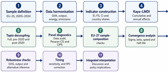
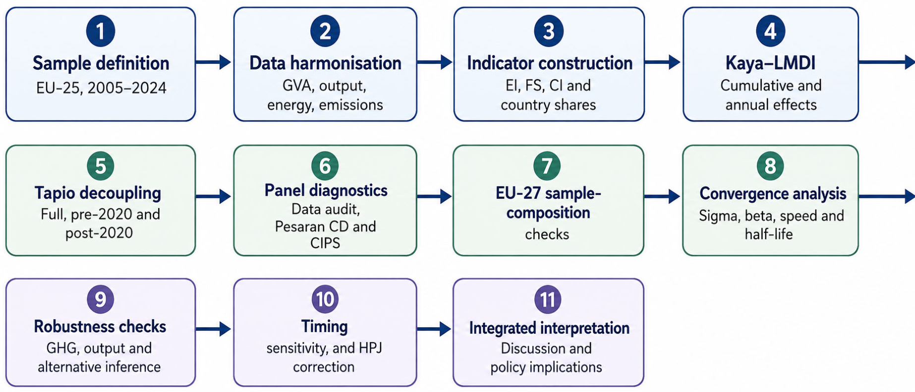
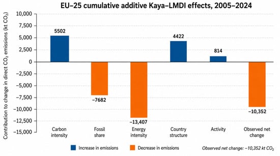
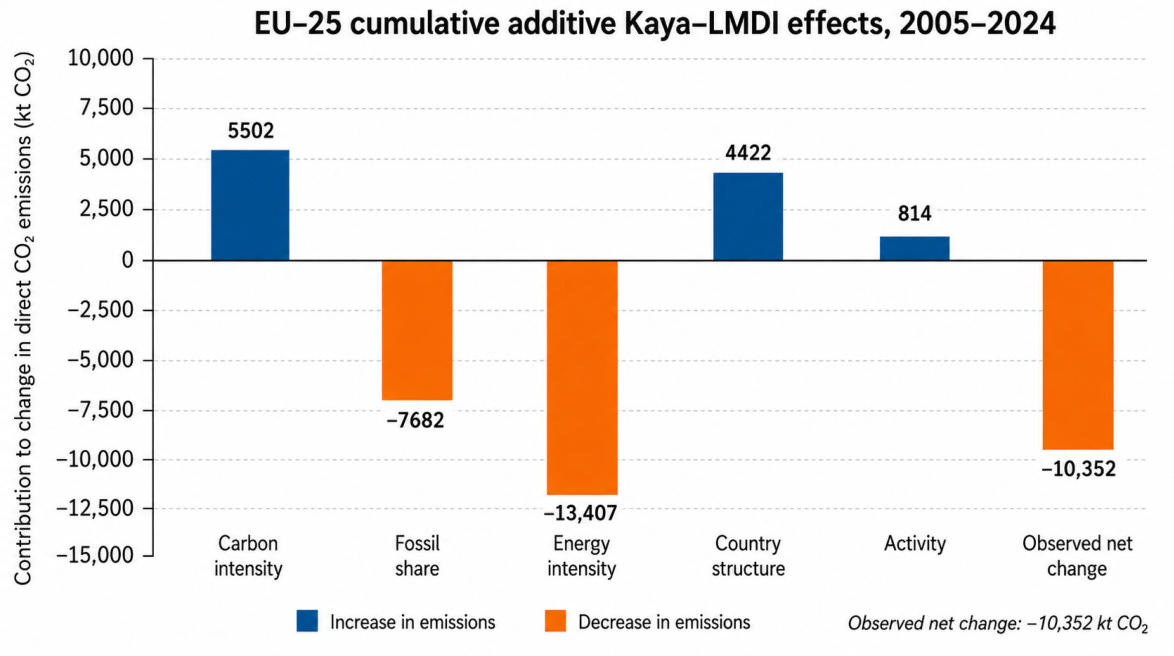
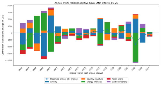
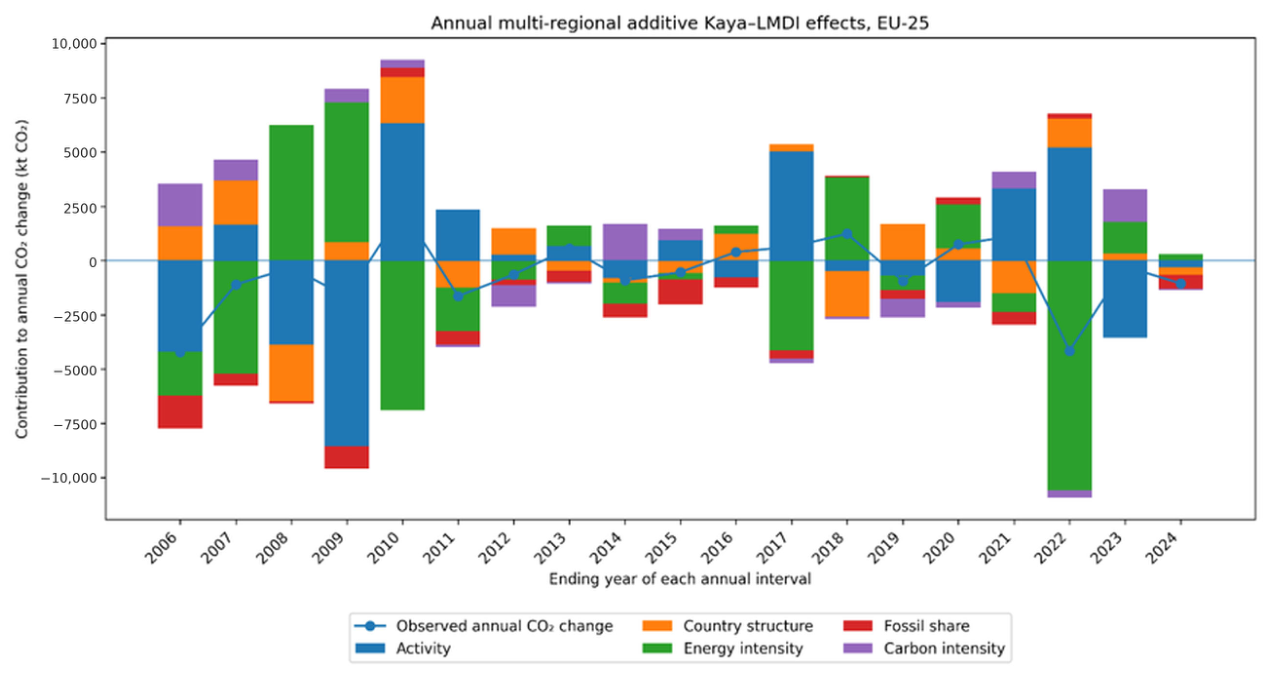
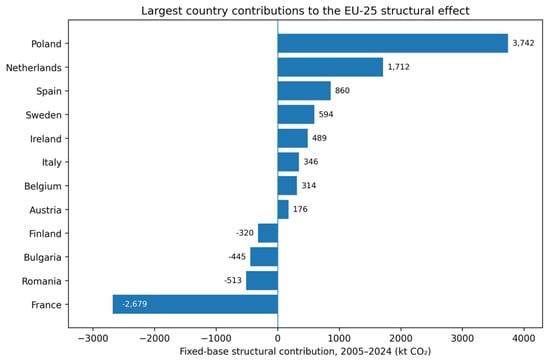
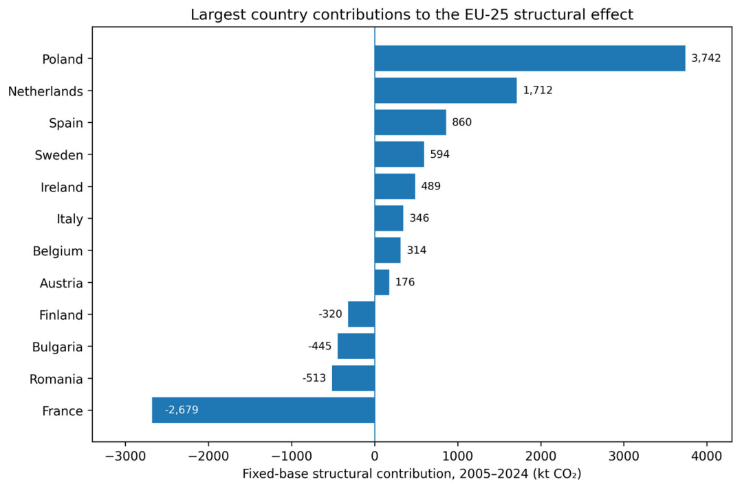

Disclaimer/Publisher’s Note: The statements, opinions and data contained in all publications are solely those of the individual author(s) and contributor(s) and not of MDPI and/or the editor(s). MDPI and/or the editor(s) disclaim responsibility for any injury to people or property resulting from any ideas, methods, instructions or products referred to in the content. |
© 2026 by the authors. Licensee MDPI, Basel, Switzerland. This article is an open access article distributed under the terms and conditions of the Creative Commons Attribution (CC BY) license.