Mean Shift Test-Based Identification of Severe Missing Events in Low-Voltage Distribution Networks

Abstract

To identify severe missing events in low-voltage distribution network (LVDN) measurements under coexisting errors and asynchrony, a label-free severe missing event detection method based on the mean shift test is proposed. First, mathematical models for the error rate, asynchrony rate, and missing rate are established to describe typical gray measurement data scenarios in LVDNs, where errors and asynchrony are treated as background disturbances. Second, a phase-specific current regression model for severe missing-event detection is constructed based on the multiple linear relationship between the phase-line head-end current and the customer-side currents. Then, the mean shift test is introduced to detect abnormal time snapshots caused by severe missing events through statistical hypothesis testing. Simulation results show that the proposed method achieves a high TPR while maintaining a low FPR in the main comparative experiments, and it achieves the best overall TPR–FPR trade-off among the evaluated methods. The results demonstrate that the proposed method provides an effective means for label-free detection of severe missing events in LVDNs under background measurement disturbances and the operating conditions considered in this study.

1. Introduction

With the continuous advancement of new-type power system construction, a massive number of terminal devices, such as distributed photovoltaics and electric vehicle charging piles, have been widely connected to LVDNs. The quality of measurement data from these devices has thus become critical to ensuring that the operating states of LVDNs are observable, measurable, controllable, and adjustable. However, in actual operation, limited by factors such as sensor accuracy, communication interference, and environmental noise, LVDN measurement data exhibit typical “gray data” characteristics [1]; that is, the data are contaminated with various quality defects, including errors, asynchrony, and missing. Such complex data issues significantly increase the difficulty of performing LVDN topology identification, state estimation, and source–grid–load coordinated control, and they have become a major bottleneck restricting the refined perception and intelligent operation of LVDNs.

Recent studies on gray measurement data in distribution networks have shown that incomplete, distorted, and abnormal measurements can be modeled, identified, and recovered by combining statistical learning, physical constraints, and intelligent algorithms. For measurement modeling, pseudo-measurement construction and physics-informed data compensation have been widely used to improve distribution network observability and alleviate the impact of insufficient measurements [2,3]. Data-driven generative models have also been introduced to characterize uncertain data distributions and enrich scarce or imbalanced samples, thereby providing useful support for gray-data feature representation [4]. In terms of gray-data identification, existing studies mainly focus on detecting bad measurements, erroneous active power data, abnormal operating conditions, and anomalous electricity usage. Representative methods include Bayesian-network-based error detection, compressive-sensing-based online bad data identification, robust state estimation considering both measurement and topology errors, and LVDN-oriented fault or bad-data diagnosis methods [5,6,7,8,9,10]. More recently, deep learning and spatiotemporal modeling techniques, such as Transformer-based anomaly detection, graph neural networks, LSTM, GANs, and hybrid models, have further improved the ability to identify complex abnormal patterns in smart-meter and distribution network data [11,12,13]. For gray-data cleaning, missing-data imputation, distorted-data recovery, and anomalous-data reconstruction have been investigated through matrix completion, time snapshots forecasting, generative adversarial learning, 3D-CNN-based completion, gated adversarial interpolation, and denoising autoencoders [3,14,15,16,17,18]. These studies provide an important foundation for enhancing the availability and reliability of distribution network measurement data. However, their main objective is usually to compensate missing values, detect general bad data, or reconstruct corrupted measurements, rather than to identify severe missing events that may fundamentally destroy the statistical relationship between transformer-side, phase-line, and customer-side measurements. In practical LVDNs, missing, errors, asynchrony, and abnormal fluctuations may coexist, causing current-based topology identification or state awareness models to draw unreliable conclusions. Therefore, before applying topology identification, phase identification, or other measurement-driven state awareness methods, it is necessary to diagnose severe missing events hidden in the measurement data.

Recent studies on LVDN topology identification have shown that smart-meter measurements can be used to infer customer–branch connections, customer phase relationships, and confidence-aware topology information. Data-driven methods have been developed for customer–branch connectivity identification [19], phase identification under incomplete data conditions [20], and weakly supervised multi-source fusion for confidence-aware topology identification [21]. These studies provide an important basis for exploiting the statistical relationship between transformer-side or phase-line measurements and customer-side measurements. However, their main objective is topology identification rather than data-quality diagnosis. In practical LVDNs, errors, asynchrony, and missing may coexist and distort the current-based relationship used by these topology identification methods. Therefore, before applying topology identification or state awareness models, it is necessary to identify severe missing events hidden in the measurement data.

Overall, existing studies have made progress in pseudo-measurement modeling, bad-data detection, anomaly identification, missing-data imputation, and topology identification. However, most of these methods are designed for generic bad-data detection, data reconstruction, or topology inference, rather than for identifying hidden severe missing events in LVDN measurement systems. In practical LVDNs, small errors and asynchrony usually coexist with more severe missing events caused by electricity theft or communication anomalies. These background disturbances may weaken the regression relationship between the phase-line head-end current and customer-side currents, making missing detection more difficult. Meanwhile, learning-based methods often require a large number of labeled abnormal samples, while many residual- or influence-based diagnostic methods lack a direct physical interpretation for LVDN current measurements. Therefore, there remains a need for an interpretable and label-free statistical method for detecting severe missing events in LVDNs under coexisting errors and asynchrony.

To this end, this paper proposes a severe missing-event detection method for LVDNs based on the mean shift test. First, mathematical models for the error rate, asynchrony rate, and missing rate in LVDN gray measurement data are established. Second, a phase-specific current regression model for severe missing-event detection for LVDNs is constructed based on multiple linear regression. Finally, the mean shift test algorithm is introduced to achieve statistical identification of time snapshots through hypothesis testing. In this paper, errors and asynchrony are treated as background disturbances, and the focus is on detecting time snapshots affected by severe missing events induced by electricity theft or communication anomalies, rather than classifying the exact anomaly cause. The main contributions of this paper are as follows:

(a)

A scenario-oriented gray measurement model is established to distinguish background disturbances from severe missing mechanisms in LVDNs.

(b)

An interpretable current regression representation is developed to link missing events with mean shifts in the relationship between phase-line head-end current and customer-side currents.

(c)

A standard mean shift test is adapted into a label-free diagnostic procedure for detecting severe missing events in LVDNs without requiring abnormal training samples.

2. Materials and Methods

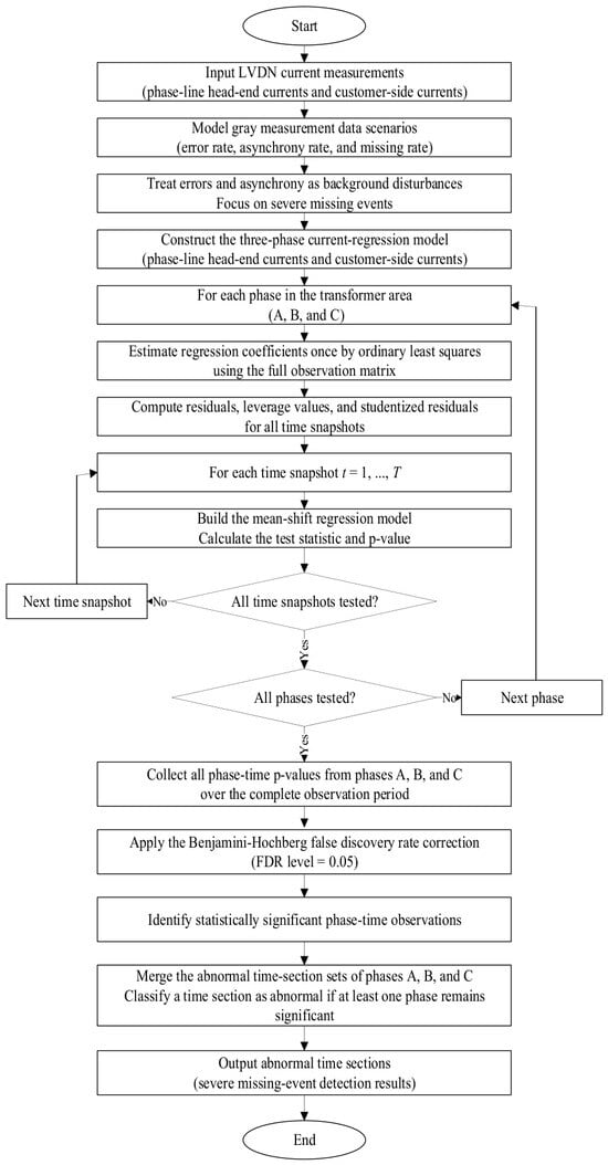
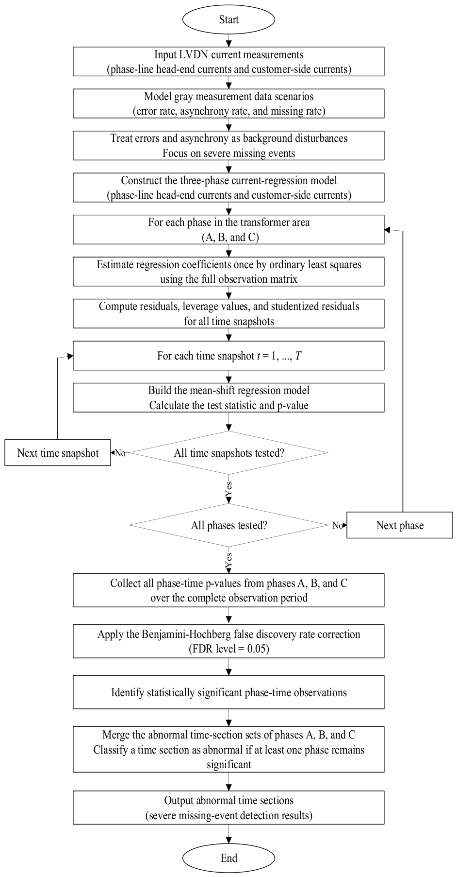
To improve the readability of the proposed methodology, Figure 1 presents the overall workflow of the proposed mean shift test-based severe missing-event detection method under background measurement disturbances.

Figure 1. Overall workflow of the proposed mean shift test-based identification method for severe missing events in LVDNs.

2.1. Problem Description

The gray measurement data in LVDNs mainly manifest as errors, asynchrony, and missing. To facilitate subsequent modeling and identification, this paper adopts the error rate, asynchrony rate, and missing rate to quantitatively characterize the above three types of gray data features.

Before modeling the measurement error rate and asynchrony rate, the distributional assumptions are clarified. Following previous smart-meter-data-based topology and phase identification studies [1,22], random metering errors and synchronization errors are modeled as zero-mean Gaussian disturbances in the baseline case. This assumption provides a tractable approximation for small random deviations around calibrated meter readings and reference sampling instants. The zero mean indicates no persistent directional bias after calibration or synchronization correction, while the variance reflects the disturbance level related to meter accuracy or clock deviation. Nevertheless, this is an idealized baseline assumption, and practical LVDNs may still involve metering bias, clock drift, communication delay, data aggregation effects, and non-Gaussian disturbances. Their influence is further examined in the robustness analysis.

2.1.1. Error Rate

The error rate of load measurement data is defined as the relative deviation between the measured load value and the true value at a given time instant, caused by the metering error of the customer meter or measurement terminal. It can be represented by the variable ${\epsilon }_{\mathrm{e}}$, and its calculation formula is given as follows:

$${\epsilon }_{\mathrm{e}}={\displaystyle \frac{X_{\mathrm{me}\left(\mathrm{e}\right)}-X_{\mathrm{tu}\left(\mathrm{e}\right)}}{X_{\mathrm{tu}\left(\mathrm{e}\right)}}}={\displaystyle \frac{\Delta X_{(\mathrm{e})}}{X_{\mathrm{tu}\left(\mathrm{e}\right)}}},$$

(1)

where $X_{\mathrm{m}\mathrm{e}(\mathrm{e})}$ represents the load measurement value of the customer meter or measurement terminal; $X_{\mathrm{tu}(\mathrm{e})}$ represents the true load value at the given time instant; and $\Delta X_{(\mathrm{e})}$ represents the metering error resulting from the insufficient metering accuracy of the customer meter or measurement terminal.

The metering deviation is objective and its magnitude is related to the accuracy class of the meter and measurement terminal. It can generally be assumed that ${\epsilon }_{\mathrm{e}}$ follows a normal distribution with an expected value of zero, and its standard deviation ${\sigma }_{\mathrm{e}}$ is related to the accuracy class of the meter or measurement terminal.

$${\epsilon }_{\mathrm{e}}~N(0,{\sigma }_{\mathrm{e}}^2),$$

(2)

$${\sigma }_{\mathrm{e}}=\omega /3,$$

(3)

where $\omega$ denotes the accuracy class of the meter or measurement terminal, typically classes 0.2, 1, 2, and 5. Different classes indicate the maximum error range of the metering data; for example, class 0.2 provides the highest accuracy with an error range of ±0.2%, while class 5 has the lowest accuracy with an error range of ±5%. Accordingly, the numerical range of ${\sigma }_{\mathrm{e}}$ is approximately 0.1% to 1.7%.

The factor 1/3 is adopted according to the three-sigma approximation, where the meter accuracy class is treated as an approximate maximum relative error bound and the standard deviation is set so that most random deviations fall within this bound under the baseline Gaussian assumption.

From the above, the error rate of load measurement data is a random variable that follows a normal distribution. Therefore, the error level of the data is generally judged by the standard deviation of the error rate of the measurement data; that is, a larger standard deviation of the error rate implies a greater possible magnitude of deviation of the measured value from the true value and a larger measurement data error, and vice versa.

In the simulation experiments of this paper, biased and non-Gaussian perturbations are additionally examined in separate sensitivity experiments, thereby ensuring that the evaluation is not restricted to zero-mean Gaussian perturbations.

2.1.2. Asynchrony-Induced Equivalent Disturbance

Smart-meter data used in this study are interval measurements that have been preliminarily aligned to common nominal sampling instants. Therefore, the temporal asynchrony considered here refers to the small residual clock deviation remaining after routine time alignment, rather than an arbitrary displacement of the complete load curve. Previous data-driven LVDN studies have constructed topology-related statistical relationships using aligned smart-meter time snapshot measurements [19,22]. In addition, asynchronous timestamps have been considered as a source of measurement uncertainty in distribution-grid estimation [23].

Let $\Delta t_j(t)$ denote the residual clock offset of customer j relative to the nominal sampling instant t. The recorded value is physically associated with the current at the shifted time $t+\Delta t_j(t)$. Therefore, the relative deviation induced by temporal asynchrony is expressed as

$${\eta }_{a,j}(t)={\displaystyle \frac{X_{\mathrm{true},j}(t+\Delta t_j(t))-X_{\mathrm{true},j}(t)}{X_{\mathrm{true},j}(t)}},$$

(4)

When the residual clock offset is sufficiently small and the load trajectory is locally smooth within the sampling interval, a first-order approximation gives

$${\eta }_{a,j}(t)\approx {\kappa }_j(t){\displaystyle \frac{\Delta t_j(t)}{t_{\mathrm{interval}}}},\hspace{1em}{\kappa }_j(t)={\displaystyle \frac{t_{\mathrm{interval}}}{X_{\mathrm{true},j}(t)}}{\displaystyle \frac{\mathrm{d}{X}_{\mathrm{true},j}(t)}{\mathrm{d}t}},$$

(5)

where $t_{\mathrm{interval}}$ is the nominal sampling interval and ${\kappa }_j(t)$ is a dimensionless coefficient characterizing the local variation in the customer load. Equation (5) shows that the ratio between the clock offset and the sampling interval is only a normalized temporal-displacement index; the resulting relative current deviation also depends on the local load-variation rate.

In the simulation, the detailed variation of ${\kappa }_j(t)$ is absorbed into an equivalent disturbance parameter. The asynchrony-induced disturbance in the baseline case is modeled as

$${\eta }_{a,j}(t)~N(0,{\sigma }_a^2),\hspace{1em}0\le {\sigma }_a\le {\kappa }_a{\displaystyle \frac{\Delta t_{\max }}{t_{\mathrm{interval}}}},$$

(6)

where ${\kappa }_a$ is the equivalent load-variation sensitivity coefficient and $\Delta t_{\max }$ is the maximum residual clock offset considered. A normalized conservative setting of ${\kappa }_a=1$ is adopted in the baseline simulation. With a sampling interval of 15 min and a residual clock offset not exceeding 1 min, the equivalent disturbance level is set within 0–6.7%.

It should be emphasized that 6.7% represents the upper level of the normalized equivalent disturbance used in the robustness experiment, rather than an exact conversion from a 1 min clock offset to a relative current error. This approximation applies to interval measurements with small residual clock offsets and locally smooth load variations. Large clock shifts, switching transients, and abrupt load changes are outside the scope of the baseline model. The specific baseline disturbance standard deviation used in the simulations is given in Section 3.2 and is lower than this upper bound.

2.1.3. Missing Rate

To distinguish the complete measurement from the measurement actually retained in the dataset, $X_{\mathrm{ref}}(t,j)$ denotes the reference current measurement of customer j at time t in the absence of the considered severe missing event. The reference measurement may still contain the background errors and asynchrony considered in this study. Therefore, the missing amount represents only the additional data loss caused by the corresponding severe missing mechanism.

Let $\Delta X_f(t,j), \Delta X_d(t,j), \mathrm{and} \Delta X_c(t,j)$ denote the missing amounts of customer j at time t caused by electricity theft, file omission, and communication anomalies, respectively. The overall missing rate is defined as

$${\delta }_m={\displaystyle \frac{{\displaystyle \sum _{t\in \mathcal{T}}{\displaystyle \sum _{j\in \mathcal{C}}\left[\Delta X_f(t,j)+\Delta X_d(t,j)+\Delta X_c(t,j)\right]}}}{{\displaystyle \sum _{t\in \mathcal{T}}{\displaystyle \sum _{j\in \mathcal{C}}{X}_{\mathrm{ref}}}}(t,j)}},$$

(7)

where C is the set of all customers in the transformer area and T is the set of all sampling instants. When the three missing mechanisms act on mutually exclusive customer–time observations, as assumed in the simulation scenarios of this study, the overall missing rate can be decomposed as

$${\delta }_m={\delta }_f+{\delta }_d+{\delta }_c,$$

(8)

(1) Electricity-Theft-Induced Missing Rate

The missing rate caused by electricity theft is defined as

$${\delta }_f={\displaystyle \frac{{\displaystyle \sum _{t\in \mathcal{T}}{\displaystyle \sum _{j\in \mathcal{C}}\Delta }}{X}_f(t,j)}{{\displaystyle \sum _{t\in \mathcal{T}}{\displaystyle \sum _{j\in \mathcal{C}}{X}_{\mathrm{ref}}}}(t,j)}},$$

(9)

where

$$\Delta X_f(t,j)={\varphi }_f(t,j)\left(1-{\epsilon }_f\right)X_{\mathrm{ref}}(t,j),$$

(10)

Here, ${\varphi }_f(t,j)\in \{0,1\}$ is the electricity-theft indicator. A value of 1 indicates that customer j is affected by electricity theft at time t, whereas 0 indicates normal operation. ${\epsilon }_f\in [0,1]$ is the electricity-retention ratio. Therefore, when ${\varphi }_f(t,j)=1$, the retained measurement is ${\epsilon }_f{X}_{\mathrm{ref}}(t,j)$.

(2) File-Omission-Induced Missing Rate

The missing rate caused by file omission is defined as

$${\delta }_d={\displaystyle \frac{{\displaystyle \sum _{t\in \mathcal{T}}{\displaystyle \sum _{j\in \mathcal{C}}\Delta }}{X}_d(t,j)}{{\displaystyle \sum _{t\in \mathcal{T}}{\displaystyle \sum _{j\in \mathcal{C}}{X}_{\mathrm{ref}}}}(t,j)}},$$

(11)

where

$$\Delta X_d(t,j)={\varphi }_d(j)X_{\mathrm{ref}}(t,j),$$

(12)

Here, ${\varphi }_d(j)\in \{0,1\}$ indicates whether customer j is omitted from the customer archive of the transformer area. When ${\varphi }_d(j)=1$, the measurement of that customer is excluded from the transformer-area dataset throughout the considered period.

(3) Communication-Anomaly-Induced Missing Rate

The missing rate caused by communication anomalies is defined as

$${\delta }_c={\displaystyle \frac{{\displaystyle \sum _{t\in \mathcal{T}}{\displaystyle \sum _{j\in \mathcal{C}}\Delta }}{X}_c(t,j)}{{\displaystyle \sum _{t\in \mathcal{T}}{\displaystyle \sum _{j\in \mathcal{C}}{X}_{\mathrm{ref}}}}(t,j)}},$$

(13)

where

$$\Delta X_c(t,j)={\varphi }_c(t,j)X_{\mathrm{ref}}(t,j),$$

(14)

Here, ${\varphi }_c(t,j)\in \{0,1\}$ is the communication-anomaly indicator. A value of 1 indicates that the measurement of customer j is unavailable at time t because of a communication anomaly, whereas 0 indicates normal communication. In the data-acquisition system considered in this study, an unavailable communication record is represented by zero filling.

Equation (8) applies to the mutually exclusive missing-event scenarios considered in this study. If several mechanisms overlap at the same customer–time observation, the overall missing rate should be calculated directly from Equation (7) using the actually retained measurement, rather than by summing the three mechanism-specific rates, to avoid double counting. The reference measurements and mechanism indicators are used only for constructing and quantifying the simulation scenarios and are not required as inputs to the proposed detection method.

2.2. Phase-Specific Current Regression Model for Severe Missing-Event Detection

In a three-phase four-wire LVDN, measurement data mainly come from smart meters, which typically cannot provide phase angle information directly. Therefore, in practical applications, the root-mean-square value of current is usually used to approximately represent the active current component. This approximation inevitably introduces a modeling discrepancy, denoted as e(t). Consequently, the relationship between the phase-line head-end current and the currents of the customer nodes it supplies can be expressed as:

$$I_0(t)=\sum _{j\in C}{I}_j(t)+e(t),$$

(15)

where C represents the set of customer nodes; I₀(t) denotes the measured current at the phase-line head-end; I_j(t) denotes the measured current of the j-th customer node; and e(t) is the regression error term that aggregates the RMS-current approximation error and other unmodeled disturbances. It can be seen from the above equation that a significant multiple linear correlation exists between the phase-line head-end current and the currents of the downstream customer nodes, which provides a theoretical basis for severe missing-event detection based on regression analysis.

It should be noted that Equation (15) is a statistical approximation based on routinely available RMS-current measurements rather than an exact phasor-current equation. Its applicability is limited to operating periods with relatively stable voltage magnitudes, relatively high and slowly varying customer power factors, limited current-angle dispersion within each phase, phase imbalance within the range represented by the considered test systems, and no frequent or substantial PV-induced reverse power flow. Strongly time-varying power factors, large angle dispersion, or current-direction reversals may alter the conditional mean relationship rather than merely increasing the residual variance. Such operating conditions are outside the validated scope of the present study.

For ease of illustration, phase A is taken as an example for modeling below; phase B and phase C can be handled in the same way. Let the phase-A line head-end current be the dependent variable I_YA, and the currents of the N_A customer nodes connected to phase A be the independent variables $I_{\mathrm{X}\mathrm{A}1},\cdots ,I_{\mathrm{X}\mathrm{A}N}$. Then, the relationship between them is as follows:

$$I_{\mathrm{Y}\mathrm{A}}={\alpha }_{\mathrm{A}1}{I}_{\mathrm{X}\mathrm{A}1}+{\alpha }_{\mathrm{A}2}{I}_{\mathrm{X}\mathrm{A}2}+\dots +{\alpha }_{\mathrm{A}{N}_{\mathrm{A}}}{I}_{\mathrm{X}\mathrm{A}{N}_{\mathrm{A}}}+e_{\mathrm{A}},$$

(16)

Equation (16) is a multiple linear regression model, where ${\alpha }_{\mathrm{A}1},{\alpha }_{\mathrm{A}2},\cdots {\alpha }_{\mathrm{A}{N}_{\mathrm{A}}}$ represents the regression model parameters, also known as regression coefficients. The fitted regression relationship provides the baseline against which residual mean shifts are evaluated.

If T_A observations are made on $I_{\mathrm{YA}},I_{\mathrm{XA}1},\cdots ,I_{\mathrm{XA}{N}_{\mathrm{A}}}$, yielding T_A sets of observed values:

$$I_{\mathrm{XA}t1},\dots ,I_{\mathrm{XA}t{N}_{\mathrm{A}}},I_{\mathrm{YA}t},t=1,\dots ,T_{\mathrm{A}},$$

(17)

They satisfy the relationship:

$$I_{\mathrm{YA}t}={\alpha }_{\mathrm{A}1}{I}_{\mathrm{X}\mathrm{A}t1}+{\alpha }_{\mathrm{A}2}{I}_{\mathrm{X}\mathrm{A}t2}+\dots +{\alpha }_{\mathrm{A}{N}_{\mathrm{A}}}{I}_{\mathrm{X}\mathrm{A}t{N}_{\mathrm{A}}}+e_{\mathrm{A}t},t=1,\dots ,T_{\mathrm{A}},$$

(18)

Here, e_At denotes the model error at time t. Introducing matrix notation:

$${\mathit{I}}_{\mathbf{Y}\mathbf{A}}=\left[\begin{array}{c}{I}_{\mathrm{Y}\mathrm{A}1}\\ I_{\mathrm{Y}\mathrm{A}2}\\ ⋮\\ I_{\mathrm{Y}\mathrm{A}{T}_{\mathrm{A}}}\end{array}\right],{\mathit{I}}_{\mathbf{X}\mathbf{A}}=\left[\begin{array}{ccc}{I}_{\mathrm{X}\mathrm{A}11}& \cdots & I_{\mathrm{X}\mathrm{A}1N_{\mathrm{A}}}\\ ⋮& \ddots & ⋮\\ I_{\mathrm{X}\mathrm{A}{T}_{\mathrm{A}}1}& \cdots & I_{\mathrm{X}\mathrm{A}{T}_{\mathrm{A}}{N}_{\mathrm{A}}}\end{array}\right],{\mathit{\alpha }}_{\mathbf{A}}=\left[\begin{array}{c}{\alpha }_{\mathrm{A}1}\\ {\alpha }_{\mathrm{A}2}\\ ⋮\\ {\alpha }_{\mathrm{A}{N}_{\mathrm{A}}}\end{array}\right],{\mathbf{e}}_{\mathrm{A}}=\left[\begin{array}{c}{e}_{\mathrm{A}1}\\ e_{\mathrm{A}2}\\ ⋮\\ e_{\mathrm{A}{T}_{\mathrm{A}}}\end{array}\right],$$

(19)

Then Equation (18) can be written in the following compact form:

$${\mathit{I}}_{\mathbf{Y}\mathbf{A}}={\mathit{I}}_{\mathbf{X}\mathbf{A}}{\mathit{\alpha }}_{\mathbf{A}}+{\mathit{e}}_{\mathbf{A}},$$

(20)

where ${\mathit{I}}_{\mathbf{Y}\mathbf{A}}$ is the T_A times 1 observation vector of the phase-line head-end current, ${\mathit{I}}_{\mathbf{X}\mathbf{A}}$ is the T_A times N_A observation matrix of the currents of customer nodes connected to phase A, ${\mathit{\alpha }}_{\mathbf{A}}$ is the N_A times 1 vector of unknown regression coefficients, and ${\mathit{e}}_{\mathbf{A}}$ is the T_A times 1 model error vector.

For a complete three-phase LVDN, this paper assumes that the numbers of customer nodes connected to phases A, B, and C are N_A, N_B, and N_C respectively. It is also assumed that T_A, T_B, and T_C observations are made on the three-phase current quantities respectively. Then, introducing matrix notation:

$${\mathit{I}}_{\mathbf{Y}}=\left[\begin{array}{ccc}{I}_{\mathrm{Y}\mathrm{A}1}& 0& 0\\ ⋮& ⋮& ⋮\\ I_{{\mathrm{Y}\mathrm{A}T}_{\mathrm{A}}}& 0& 0\\ 0& I_{\mathrm{Y}\mathrm{B}1}& 0\\ ⋮& ⋮& ⋮\\ 0& I_{\mathrm{Y}\mathrm{B}{T}_{\mathrm{B}}}& 0\\ 0& 0& I_{\mathrm{Y}\mathrm{C}1}\\ ⋮& ⋮& ⋮\\ 0& 0& I_{\mathrm{Y}\mathrm{C}{T}_{\mathrm{C}}}\end{array}\right],$$

(21)

$${\mathit{I}}_{\mathbf{X}}=\left[\begin{array}{ccccccccc}{I}_{\mathrm{X}\mathrm{A}11}& \cdots & I_{\mathrm{X}\mathrm{A}1N_{\mathrm{A}}}& 0& \cdots & 0& 0& \cdots & 0\\ ⋮& \ddots & ⋮& ⋮& \ddots & ⋮& ⋮& \ddots & ⋮\\ I_{\mathrm{X}\mathrm{A}{T}_{\mathrm{A}}1}& \cdots & I_{\mathrm{X}\mathrm{A}{T}_{\mathrm{A}}{N}_{\mathrm{A}}}& 0& \cdots & 0& 0& \cdots & 0\\ 0& \cdots & 0& I_{\mathrm{X}\mathrm{B}11}& \cdots & I_{\mathrm{X}\mathrm{B}1N_{\mathrm{B}}}& 0& \cdots & 0\\ ⋮& \ddots & ⋮& ⋮& \ddots & ⋮& ⋮& \ddots & ⋮\\ 0& \cdots & 0& I_{\mathrm{X}\mathrm{B}{T}_{\mathrm{B}}1}& \cdots & I_{\mathrm{X}\mathrm{B}{T}_{\mathrm{B}}{N}_{\mathrm{B}}}& 0& \cdots & 0\\ 0& \cdots & 0& 0& \cdots & 0& I_{\mathrm{X}\mathrm{C}11}& \cdots & I_{\mathrm{X}\mathrm{C}1N_{\mathrm{C}}}\\ ⋮& \ddots & ⋮& ⋮& \ddots & ⋮& ⋮& \ddots & ⋮\\ 0& \cdots & 0& 0& \cdots & 0& I_{\mathrm{X}\mathrm{C}{T}_{\mathrm{C}}1}& \cdots & I_{\mathrm{X}\mathrm{C}{T}_{\mathrm{C}}{N}_{\mathrm{C}}}\end{array}\right],$$

(22)

$$\mathit{\alpha }=\left[\begin{array}{ccc}{\alpha }_{\mathrm{A}1}& 0& 0\\ ⋮& ⋮& ⋮\\ {\alpha }_{\mathrm{A}{N}_{\mathrm{A}}}& 0& 0\\ 0& {\alpha }_{\mathrm{B}1}& 0\\ ⋮& ⋮& ⋮\\ 0& {\alpha }_{\mathrm{B}{N}_{\mathrm{B}}}& 0\\ 0& 0& {\alpha }_{\mathrm{C}1}\\ ⋮& ⋮& ⋮\\ 0& 0& {\alpha }_{\mathrm{C}{N}_{\mathrm{C}}}\end{array}\right],$$

(23)

$$\mathit{e}=\left[\begin{array}{ccc}{e}_{\mathrm{A}1}& 0& 0\\ ⋮& ⋮& ⋮\\ e_{\mathrm{A}{T}_{\mathrm{A}}}& 0& 0\\ 0& e_{\mathrm{B}1}& 0\\ ⋮& ⋮& ⋮\\ 0& e_{\mathrm{B}{T}_{\mathrm{B}}}& 0\\ 0& 0& e_{\mathrm{C}1}\\ ⋮& ⋮& ⋮\\ 0& 0& e_{\mathrm{C}{T}_{\mathrm{C}}}\end{array}\right],$$

(24)

Then Equation (20) can be expanded into the following form:

$${\mathit{I}}_{\mathbf{Y}}={\mathit{I}}_{\mathbf{X}}\mathit{\alpha }+\mathit{e},$$

(25)

where ${\mathit{I}}_{\mathbf{Y}}$ is the (T_A + T_B + T_C) times 3 observation matrix of the phase-line head-end current, ${\mathit{I}}_{\mathbf{X}}$ is the (T_A + T_B + T_C) times (N_A + N_B + N_C) observation matrix of the currents of customer nodes connected to phases A, B, and C, $\mathit{\alpha }$ is the (N_A + N_B + N_C) times 3 matrix of unknown regression coefficients, and $\mathit{e}$ is the (T_A + T_B + T_C) times 3 model error matrix.

The structure of the regression coefficient matrix $\mathit{\alpha }$ directly reflects the correspondence between customer nodes and the three-phase lines. Ideally, if a customer is actually connected to a certain phase, its corresponding regression coefficient should be significantly nonzero in the column corresponding to that phase and close to zero in the other two columns. Therefore, the numerical distribution and structural characteristics of $\mathit{\alpha }$ not only contain the topology connection information of the LVDN but are also highly sensitive to gray measurement data. When gray data issues such as measurement errors, temporal asynchrony, or data missing exist, the theoretical structure of the regression coefficients will deviate, resulting in abnormal fluctuations or deviations in the coefficient estimation results.

2.3. Mean Shift Test-Based Severe Missing-Event Detection Method

Under the condition that the regression coefficients are unknown, the error distribution of the phase-specific current regression model cannot be directly observed. Therefore, to understand the error characteristics of the regression model, the estimated value of the error, i.e., the residual, is generally used for analysis in practical applications. For any one of phases A, B, and C, and for the multiple linear regression model of low-voltage topology identification given by Equation ${\mathit{I}}_{\mathbf{Y}\mathbf{A}}={\mathit{I}}_{\mathbf{X}\mathbf{A}}{\mathit{\alpha }}_{\mathbf{A}}+{\mathit{e}}_{\mathbf{A}}$, it is written in a simplified form as ${\mathit{I}}_{\mathbf{Y}}={\mathit{I}}_{\mathbf{X}}\mathit{\alpha }+\mathit{e}$. If I_x1, I_x2, …, I_xT denote the T row vectors of the observation matrix I_X, and I_y1, I_y2, …, I_yT denote the T elements of the observation matrix I_Y, then the residual at the t time instant is defined as:

$${\widehat{e}}_t=I_{\mathrm{y}t}-{\mathit{I}}_{\mathbf{x}\mathit{t}}\widehat{\mathit{\alpha }},t=1,\dots ,T,$$

(26)

where $\widehat{\mathit{\alpha }}$ is the ordinary least squares estimate vector of $\mathit{\alpha }$, $\widehat{\mathit{\alpha }}={({\mathit{I}}_{\mathbf{X}}^{\prime }{\mathit{I}}_{\mathbf{X}})}^{-1}{\mathit{I}}_{\mathbf{X}}^{\prime }{\mathit{I}}_{\mathbf{Y}}$.

To better compare the magnitude of residuals across time snapshots, in practical applications the residual ${\widehat{e}}_t$ is usually standardized to obtain the studentized residual r_t, i.e.,

$$r_t={\displaystyle \frac{{\widehat{e}}_t}{\widehat{\sigma }\sqrt{1-h_{\mathrm{tt}}}}},t=1,\dots ,T,$$

(27)

where $\widehat{\sigma }=\sqrt{{\displaystyle \sum _{t=1}^N{\widehat{e}}_t^2}/(T-N)}$ is the estimated value of the error variance, and h_tt is the t-th diagonal element of the hat matrix $\mathit{H}={\mathit{I}}_{\mathbf{X}}{({\mathit{I}}_{\mathbf{X}}^{\prime }{\mathit{I}}_{\mathbf{X}})}^{-1}{\mathit{I}}_{\mathbf{X}}^{\prime }$.

For the regression model given as ${\mathit{I}}_{\mathbf{Y}}={\mathit{I}}_{\mathbf{X}}\mathit{\alpha }+\mathit{e}$, if the t-th set of sample data (I_xt, I_yt) is an outlier, then its residual value should be significantly large. The reason for the above situation is that the mean E(I_yt) has undergone a non-random shift τ, in which case a new regression model can be obtained:

$$\left\{\begin{array}{l}{I}_{\mathrm{y}i}={\mathit{I}}_{\mathbf{x}\mathit{i}}\mathit{\alpha }+e_i,i\ne t\\ I_{\mathrm{y}t}={\mathit{I}}_{\mathbf{x}\mathit{t}}\mathit{\alpha }+\tau +e_t,e_t~N(0,{\sigma }^2)\end{array}\right.,$$

(28)

Let d = (0, …, 0, 1, 0, …, 0)’ be a T-dimensional vector with the t-th element equal to 1 and all other elements equal to 0. Then the regression model ${\mathit{I}}_{\mathbf{Y}}={\mathit{I}}_{\mathbf{X}}\mathit{\alpha }+\mathit{e}$ can be rewritten in matrix form as:

$${\mathit{I}}_{\mathbf{Y}}={\mathit{I}}_{\mathbf{X}}\mathit{\alpha }+{\mathit{d}}_{\mathit{t}}\tau +\mathit{e},\mathit{e}~N(0,{\mathit{\sigma }}^2\mathit{I}),$$

(29)

The above model is referred to as the mean shift linear regression model. To determine that (I_xt, I_yt) is not an outlier is equivalent to testing the hypothesis H₀: τ = 0. For the mean shift linear regression model (29), the least squares estimates of $\mathit{\alpha }$ and $\tau$ are respectively:

$$\mathit{\alpha }*={\widehat{\mathit{\alpha }}}_{(t)},$$

(30)

$$\tau *={\displaystyle \frac{{\widehat{e}}_t}{1-h_{tt}}},$$

(31)

where ${\widehat{\mathit{\alpha }}}_{(t)}$ is the least squares estimate of $\mathit{\alpha }$ obtained after removing the t-th set of sample data from the regression model equation ${\mathit{I}}_{\mathbf{Y}}={\mathit{I}}_{\mathbf{X}}\mathit{\alpha }+\mathbf{e}$, ${\widehat{e}}_t$ is the t-th residual of the regression model equation ${\mathit{I}}_{\mathbf{Y}}={\mathit{I}}_{\mathbf{X}}\mathit{\alpha }+\mathit{e}$, and h_tt is the t-th diagonal element of the hat matrix $\mathit{H}={\mathit{I}}_{\mathbf{X}}{({\mathit{I}}_{\mathbf{X}}^{\prime }{\mathit{I}}_{\mathbf{X}})}^{-1}{\mathit{I}}_{\mathbf{X}}^{\prime }$.

According to the principle of hypothesis testing, if the t-th observation of the dependent variable has indeed undergone a mean shift, then in the corresponding mean shift linear regression model, the least squares estimate of the regression coefficients should equal the least squares estimate obtained after removing the t-th set of data from the original model.

To derive the test statistic for the hypothesis H₀: τ = 0, under the present setting, when the constraint τ = 0 holds in regression model (29), the residual sum of squares RSS_H can be obtained as:

$$RS{S}_H={\mathit{I}}_{\mathbf{Y}}^{\prime }{\mathit{I}}_{\mathbf{Y}}-{\widehat{\mathit{\alpha }}}^{\prime }{\mathit{I}}_{\mathbf{x}\mathit{t}}^{\prime }{\mathit{I}}_{\mathbf{Y}},$$

(32)

The unconstrained residual sum of squares RSS for regression model (29) is:

$$RSS={\mathit{I}}_{\mathbf{Y}}^{\prime }{\mathit{I}}_{\mathbf{Y}}-{\mathit{\alpha }*}^{\prime }{\mathit{I}}_{\mathbf{X}}^{\prime }{\mathit{I}}_{\mathbf{Y}}-\tau *{\mathit{d}}_{\mathit{t}}^{\prime }{\mathit{I}}_{\mathbf{Y}},$$

(33)

Based on the formulas for the least squares estimates of $\mathit{\alpha }$ and τ, denoted as $\mathit{\alpha }*$ and τ* respectively, the test statistic can be obtained as:

$$F={\displaystyle \frac{RS{S}_H-RSS}{RSS/(T-N-1)}}={\displaystyle \frac{(T-N-1)r_t^2}{T-N-r_t^2}},$$

(34)

For the mean shift linear regression model (29), if the null hypothesis H₀: τ = 0 holds, then:

$$F_t={\displaystyle \frac{(T-N-1)r_t^2}{T-N-r_t^2}}~F_{1,T-N-1},$$

(35)

For a given significance level α, if F_t > F_1,T−N−1(α), i.e., P(F_1,T−N−1 > F_t) < α, then the t-th set of observed sample data (I_xt, I_yt) is determined to be an outlier. Under the classical assumptions of independent, homoscedastic, and normally distributed regression errors, the nominal type-I error probability of an individual test is α. When these assumptions are violated, the theoretical p-value may not represent an exact finite-sample probability. Residual diagnostics are therefore conducted for the simulated cases, as reported in Section 3.2.

Because a mean shift test is performed for every time snapshot, conducting a large number of simultaneous hypothesis tests may increase the number of false-positive detections, even when the significance level of each individual test is fixed. Therefore, the Benjamini–Hochberg false discovery rate correction (BH-FDR) is incorporated as a post-processing step after the mean shift p-values are calculated. For each transformer area, all p-values obtained from phases A, B, and C over the complete observation period are treated as one family of tests and arranged in ascending order. Each ordered p-value is then compared with a rank-dependent threshold determined by its position in the ordered sequence, the total number of tests, and the prescribed FDR level, which is set to 0.05 in this study. The largest ordered p-value satisfying the BH-FDR criterion is selected as the adaptive significance cutoff, and all p-values not exceeding this cutoff are considered statistically significant. The corresponding phase–time observations are identified as abnormal, after which the abnormal time-section sets obtained for the three phases are merged. A time snapshot is ultimately classified as abnormal when at least one of its three phases remains significant after BH-FDR correction. Compared with directly comparing every p-value with a fixed significance level, under validly calibrated phase–time p-values and the dependence conditions required by the BH procedure, the BH-FDR procedure controls the expected proportion of false discoveries among the rejected phase–time hypotheses, while generally retaining greater detection capability than more conservative family-wise error rate correction methods. Because the residual diagnostics reveal departures from homoscedasticity and normality, formal FDR control is not claimed for arbitrary field data in this study. Instead, BH-FDR is used to mitigate the accumulation of false discoveries, and its practical effectiveness is evaluated through the empirical snapshot-level FPR. Therefore, it is suitable for the large number of simultaneous mean shift tests involved in LVDN time snapshots gray measurement data identification.

It should be noted that the nominal per-test significance level, the prescribed FDR level, and the empirical snapshot-level FPR are different statistical quantities. The FDR level of 0.05 controls the expected proportion of false discoveries among the phase–time hypotheses declared significant after BH-FDR correction. In contrast, the snapshot-level FPR is calculated from the final decisions after the corrected results of phases A, B, and C are merged. A time snapshot is classified as abnormal if at least one available phase remains significant after correction. Therefore, the empirical snapshot-level FPR is not expected to equal either the nominal per-test significance level or the prescribed FDR level.

It should be noted that the proposed method does not require solving a separate regression problem for each customer–time pair. For each phase, the regression coefficients are estimated once using the full observation matrix, and then the residuals, studentized residuals, leverage values, and mean shift test statistics are calculated for all time snapshots. Therefore, the method does not require $T\times N$ independent regression estimations. For one phase with T time snapshots and N customer nodes, the dominant computational complexity is approximately $O(T{N}^2+N^3)$, and the memory requirement is approximately $O(TN+N^2)$.

In practical LVDN applications, gray measurement data identification is usually performed at the transformer-area level and phase level. Thus, each computation generally involves only the customer nodes connected to one phase of one transformer area, and the number of customer nodes is usually less than 100. Under this implementation mode, the scale of each regression problem is relatively small and computationally acceptable.

For the phase-line head-end current data of phases A, B, and C, regression coefficients are calculated separately using the current data of the customers connected to their respective phases, resulting in three regression analyses in total. Subsequently, the union of the abnormal time-section sets obtained from the three analyses is taken. For any given time snapshot, as long as any one phase is identified as abnormal, that time snapshot can be determined as an abnormal time snapshot.

3. Results

3.1. Description of Case Study Parameters

The simulation experiments in this paper are conducted in two different three-phase LVDN distribution areas.

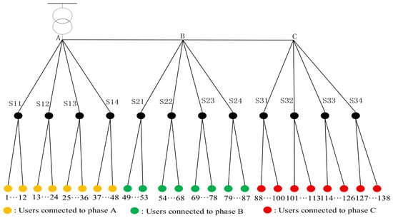
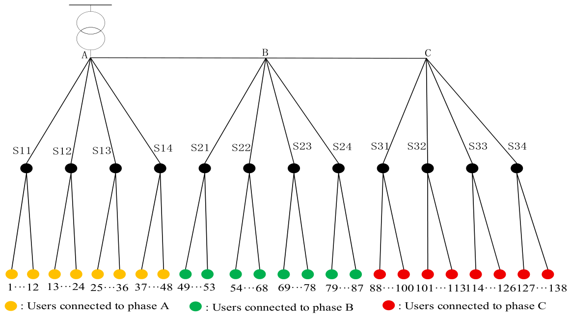
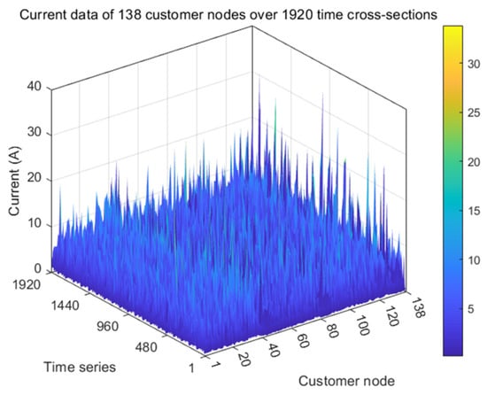
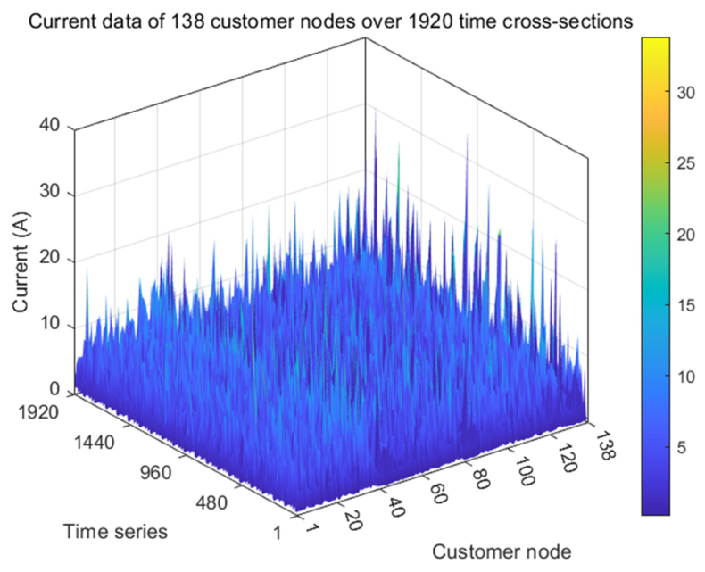
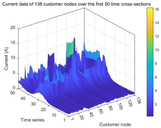
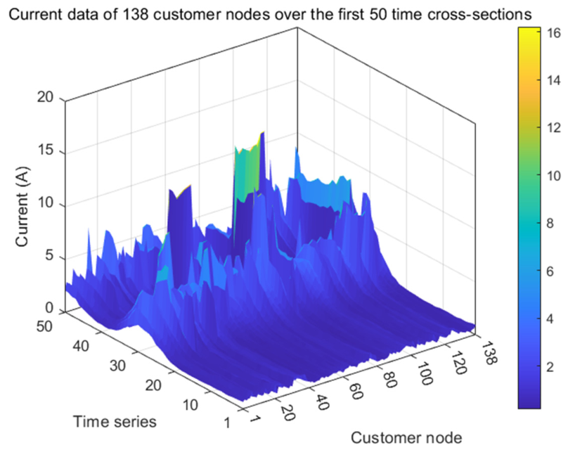
First, a typical LVDN grid structure in a Chinese rural area is considered. A three-phase test system of a rural LVDN with a total of 138 users is established, as shown in Figure 2. The data sampling interval is 15 min, and the time span is 20 days, resulting in a total of T = 1920 time snapshots. Taking the phase bus on the low-voltage side of the distribution transformer as the slack bus, multi-snapshot power flow simulations are performed to obtain the current data at each user node, as shown in Figure 3 and Figure 4.

Figure 2. The rural LVDN.

Figure 3. Current data at user nodes of the rural LVDN.

Figure 4. Current data at user nodes of the rural LVDN over the first 50 time snapshots.

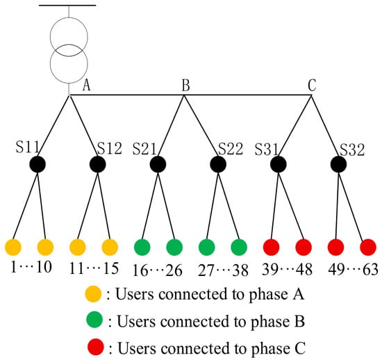
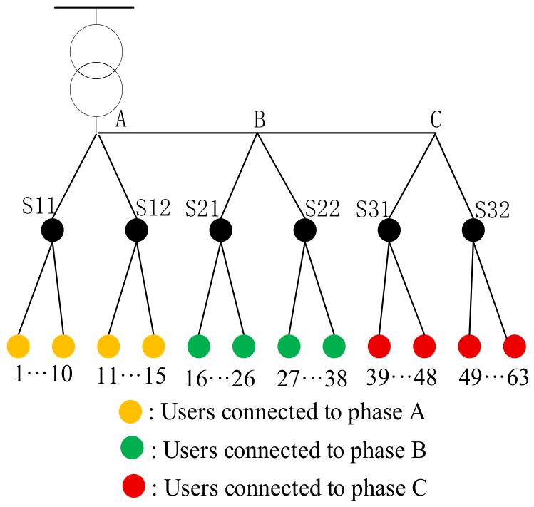
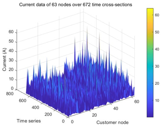
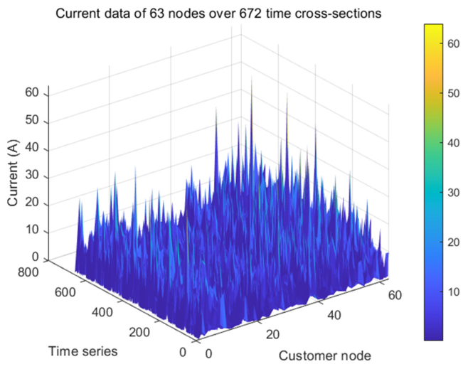
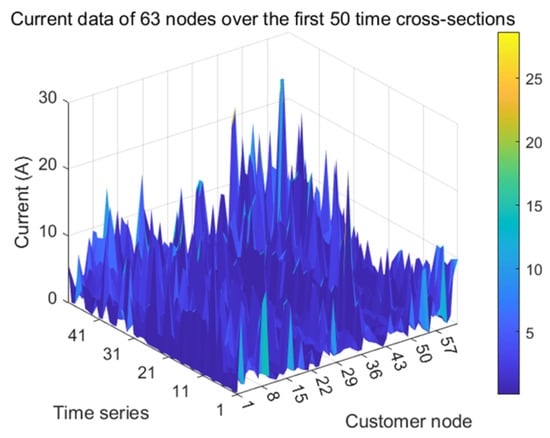
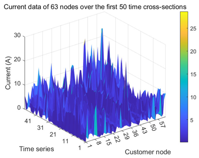
Next, a typical cable LVDN grid structure in a Chinese urban area is considered. A three-phase test system of an urban cable-type LVDN with a total of 63 users is established, as shown in Figure 5. The data sampling interval is 15 min, and the time span is 7 days, resulting in a total of T = 672 time snapshots. Taking the phase bus on the low-voltage side of the distribution transformer as the slack bus, multi-snapshot power flow simulations are performed to obtain the current data at each user node, as shown in Figure 6 and Figure 7.

Figure 5. Urban LVDN.

Figure 6. Current data at user nodes of the urban LVDN.

Figure 7. Current data at user nodes of the urban LVDN over the first 50 time snapshots.

Simulation platform: HP EliteBook x360 1040 G6; processor: Intel(R) Core(TM) i7-8565U CPU @ 1.80 GHz, 1.99 GHz; graphics card: Intel(R) UHD Graphics 620 (128 MB); operating system: Windows 10 Home China 22H2. In this paper, MATLAB 2024a is used as the simulation software for the simulation experiments.

Under this simulation platform, the single-run computation time of the proposed method is less than 5 s for the considered transformer-area-level and phase-level calculation cases.

3.2. Detection of Severe Missing Events Under Background Measurement Disturbances

To verify the capability of the proposed method in detecting time snapshots affected by severe missing events under background errors and asynchrony, simulation experiments are conducted on the above test systems. Considering that errors and asynchrony are common fundamental disturbances in low-voltage distribution networks and their impact magnitudes are typically small, errors and asynchrony are applied to the customer-side current measurements at all time snapshots over all time snapshots of all user nodes in the experiments and are not treated as the primary identification targets in this section. Meanwhile, given that file omissions occur with low probability in actual distribution areas and are more of a static record management issue, such cases are temporarily not considered in the simulations of this paper. In view of the typical operation scenarios of current low-voltage distribution areas, this paper focuses on two types of gray measurement data: electricity theft and communication anomalies.

The background noise settings are set for the two transformer areas. First, metering errors are uniformly superimposed on the customer-side currents of all users at all time snapshots. According to the accuracy class of class 2 m, the metering error is modeled as a zero-mean Gaussian random perturbation with a standard deviation of approximately 0.67%. Subsequently, equivalent perturbations caused by residual temporal asynchrony are further superimposed. Considering that the original data have already been time-aligned at a 15 min sampling interval, and assuming that the residual clock deviation does not exceed 1 min and that the equivalent load-change sensitivity is set to 1, the residual asynchrony is also modeled as a zero-mean Gaussian relative perturbation with a standard deviation of 0.67%. These two types of background disturbances are applied to all customer-side smart-meter currents throughout the entire observation period in both transformer areas. The three-phase head-end currents are treated as higher-accuracy, synchronized reference measurements in the baseline simulation, and no additional background disturbances are imposed on them. Severe missing events, such as electricity theft and communication anomalies, are then injected on this basis, whereas no additional background disturbances are superimposed on the three-phase head-end currents. The value of 0.67% is selected as a moderate baseline standard deviation within the equivalent-disturbance range of 0–6.7%. The value of 6.7% represents the upper stress-test level rather than the baseline standard deviation.

In accordance with the definitions in Section 2.1, the smart-meter measurements are first aligned to common nominal 15 min sampling instants. Residual temporal asynchrony is then represented by an equivalent relative disturbance under the assumptions of small clock offsets and locally smooth interval load variations. The normalized sensitivity coefficient is set to ${\kappa }_a=1$ in the baseline case, and the disturbance level is varied within the prescribed range. This setting is used to evaluate the influence of residual asynchrony on severe missing event detection and is not interpreted as an exact reconstruction of continuously time-shifted load trajectories.

For the missing-event scenarios, the complete simulated measurements are treated as $X_{\mathrm{ref}}(t,j)$. Electricity theft and communication anomalies are imposed through the corresponding customer–time indicators. File omission is included in the general formulation of Section 2.1 but is not simulated in the present experiments.

In this study, missing-data samples are not removed from the observation matrix and are not imputed before the mean shift test. For electricity-theft-induced missing data, the affected customer-side current is represented as a reduced nonzero reading according to the theft retention ratio. For communication-anomaly-induced missing data, the missing reading is represented as a zero-filled value according to the data acquisition convention. Therefore, the corresponding rows of the observation matrix are retained, and the proposed method detects the resulting abnormal time snapshots through the mean shift in the current regression relationship.

First, simulation experiments are conducted on the rural LVDN. The specific settings are as follows:

• User nodes 1 to 48 form an electricity theft sample block spanning time snapshots 1 to 20, and the electricity theft retention rate is set to 0.05.
• User nodes 49 to 87 form a communication anomaly sample block spanning time snapshots 1001 to 1020.
• User nodes 88 to 138 form another communication anomaly sample block spanning time snapshots 1901 to 1920.

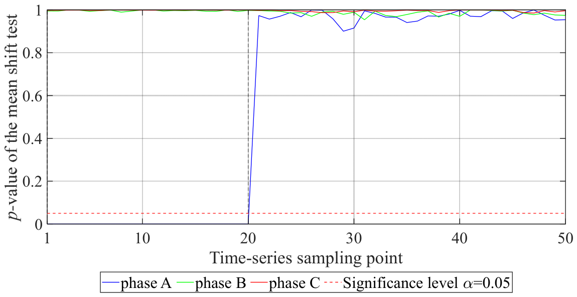
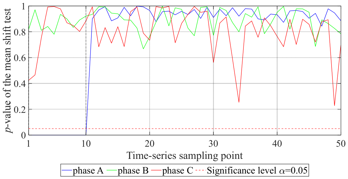
The nominal significance level for each individual mean shift test is set to α = 0.05, and the resulting phase-specific unadjusted p-values are shown in Figure 8 and Figure 9. The final detection decisions are obtained after applying the joint BH-FDR correction described in Section 2.3.

Figure 8. p-values of the mean shift test for each time snapshot of the rural LVDN.

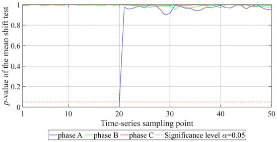
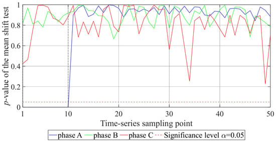
Figure 9. p-values of the mean shift test for each time snapshot over the first 50 time snapshots of the rural LVDN.

The range enclosed by the vertical dashed lines in Figure 8 refers to the time series of the set extreme abnormal gray data.

The range enclosed by the vertical dashed lines in Figure 9 refers to the time series of the set extreme abnormal gray data.

Figure 8 and Figure 9 present the unadjusted phase-specific p-values for visualization. After applying the joint BH-FDR correction to all phase–time p-values, a time snapshot is classified as anomalous if at least one phase remains statistically significant. The unadjusted p-values and final detection results for the injected anomalous time snapshots are shown in Table 1. The red and blue markings in Table 1 indicate the predefined injected labels in the simulation, rather than the automatic cause-classification results of the proposed mean shift test.

Table 1. Unadjusted p-values and final detection status for the injected anomalous time snapshots of the rural LVDN.

Time	Unadjusted Mean Shift p-Value	Detected or Not	Time	Mean Shift p-Value	Detected or Not
1	1.21 × 10−24	√	2	2.56 × 10−19	√
3	1.13 × 10−16	√	4	4.79 × 10−15	√
5	2.18 × 10−14	√	6	1.35 × 10−13	√
7	5.02 × 10−13	√	8	2.13 × 10−12	√
9	4.28 × 10−12	√	10	9.58 × 10−12	√
11	1.18 × 10−11	√	12	2.05 × 10−11	√
13	2.34 × 10−11	√	14	1.84 × 10−11	√
15	1.65 × 10−11	√	16	5.34 × 10−12	√
17	3.71 × 10−12	√	18	1.34 × 10−12	√
19	1.15 × 10−13	√	20	3.02 × 10−16	√
1001	2.47 × 10−8	√	1002	8.01 × 10−10	√
1003	1.49 × 10−11	√	1004	4.61 × 10−14	√
1005	1.53 × 10−17	√	1006	1.58 × 10−21	√
1007	2.38 × 10−29	√	1008	1.06 × 10−33	√
1009	3.93 × 10−41	√	1010	2.99 × 10−36	√
1011	4.79 × 10−41	√	1012	1.54 × 10−37	√
1013	2.42 × 10−26	√	1014	4.13 × 10−21	√
1015	1.63 × 10−17	√	1016	3.25 × 10−13	√
1017	1.32 × 10−10	√	1018	1.49 × 10−8	√
1019	1.57 × 10−7	√	1020	5.34 × 10−7	√
1901	1.90 × 10−50	√	1902	7.13 × 10−53	√
1903	9.11 × 10−52	√	1904	1.29 × 10−46	√
1905	2.05 × 10−41	√	1906	2.65 × 10−35	√
1907	3.76 × 10−29	√	1908	8.29 × 10−25	√
1909	2.71 × 10−21	√	1910	7.20 × 10−17	√
1911	2.78 × 10−14	√	1912	1.24 × 10−13	√
1913	1.36 × 10−11	√	1914	5.09 × 10−10	√
1915	1.59 × 10−8	√	1916	8.25 × 10−7	√
1917	1.63 × 10−5	√	1918	1.87 × 10−4	√
1919	0.0013	×	1920	0.0059	×

In the table, p-values reported as <2.22 × 10⁻¹⁶ are below the numerical precision limit and should not be interpreted as exactly zero.

As can be seen from Table 1, except for a few individual time snapshots (e.g., time snapshots 1919 and 1920) that were not detected, the vast majority of the time snapshots with added gray data were successfully identified. After applying the joint BH-FDR correction, 58 of the 60 injected anomalous time snapshots are detected in the rural LVDN. These results indicate that the method can detect time snapshots affected by the two injected missing-event mechanisms, but it does not automatically distinguish their physical causes.

Next, simulation experiments are conducted on the urban LVDN. The specific settings are as follows:

• User nodes 1 to 21 form an electricity theft sample block spanning time snapshots 1 to 10, the electricity theft retention rate is set to 0.01.
• User nodes 22 to 42 form a communication anomaly sample block spanning time snapshots 301 to 310.
• User nodes 43 to 63 form another communication anomaly sample block spanning time snapshots 601 to 610.

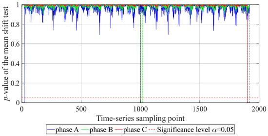
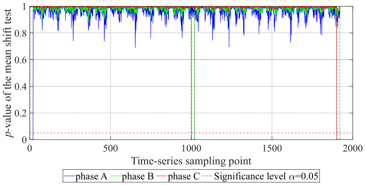
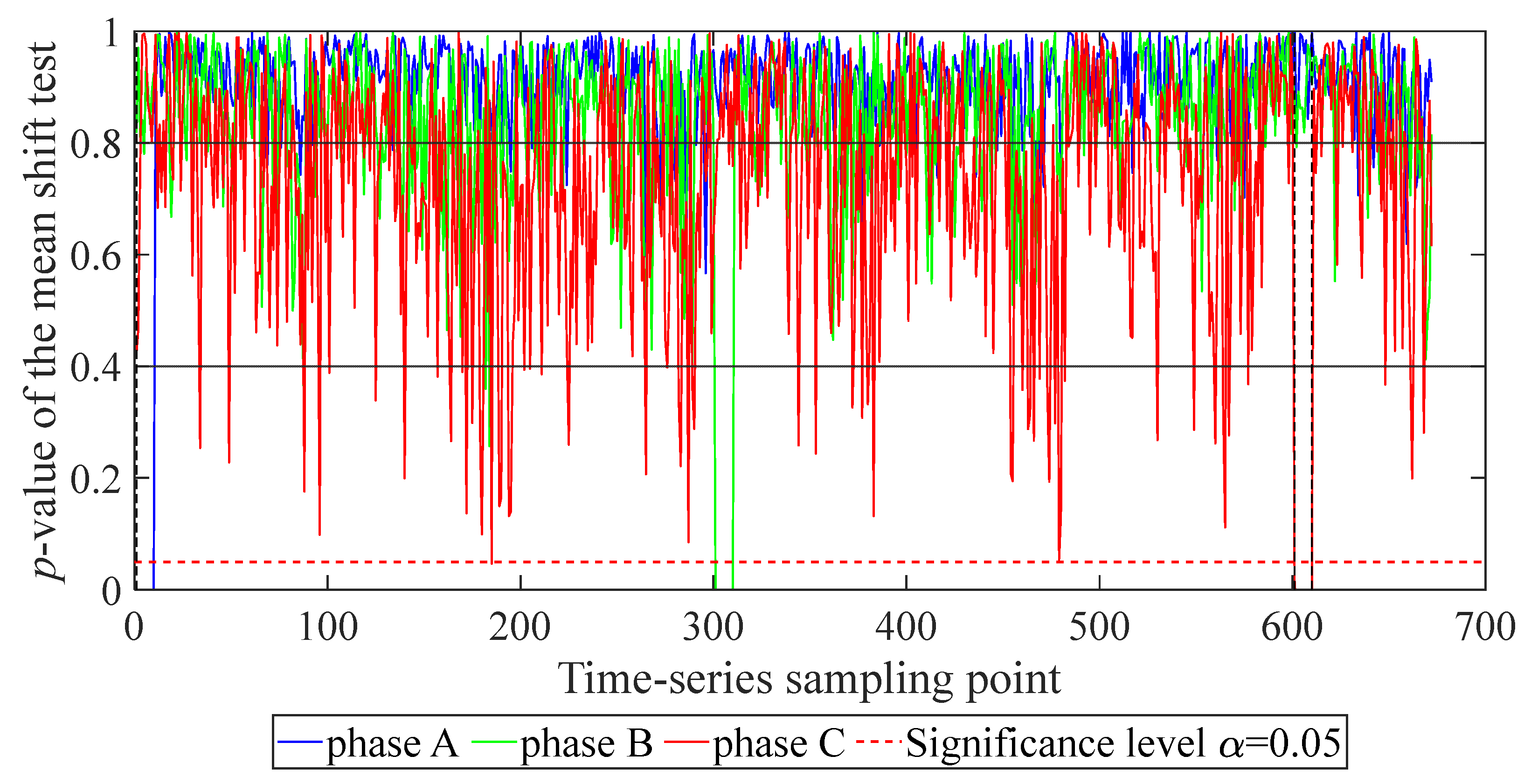
The nominal significance level for each individual mean shift test is set to α = 0.05, and the resulting phase-specific unadjusted p-values are shown in Figure 10 and Figure 11. The final detection decisions are obtained after applying the joint BH-FDR correction described in Section 2.3.

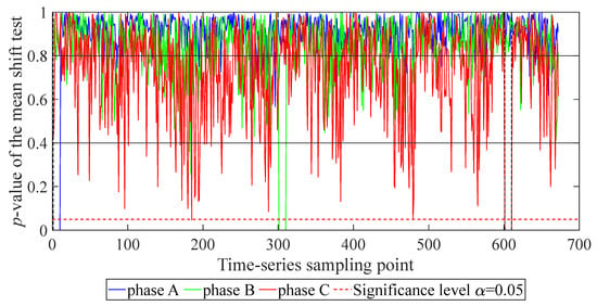
Figure 10. p-values of the mean shift test for each time snapshot of the urban LVDN.

Figure 11. p-values of the mean shift test for each time snapshot over the first 50 time snapshots of the urban LVDN.

The range enclosed by the vertical dashed lines in Figure 10 refers to the time series of the set extreme abnormal gray data.

The range enclosed by the vertical dashed lines in Figure 11 refers to the time series of the set extreme abnormal gray data.

Figure 10 and Figure 11 present the unadjusted phase-specific p-values for visualization. After applying the joint BH-FDR correction to all phase–time p-values, a time snapshot is classified as anomalous if at least one phase remains statistically significant. The total number of injected anomalous time snapshots is 30, and their corresponding calculated p-values of the mean shift test are shown in Table 2. The red and blue markings in Table 2 indicate the predefined injected labels in the simulation, rather than the automatic cause-classification results of the proposed mean shift test.

Table 2. Unadjusted p-values and final detection status for the injected anomalous time snapshots of the urban LVDN.

Time	Unadjusted Mean Shift p-Value	Detected or Not	Time	Mean Shift p-Value	Detected or Not
1	<2.22 × 10−16	√	2	1.11 × 10−16	√
3	1.21 × 10−9	√	4	7.09 × 10−8	√
5	3.22 × 10−5	√	6	2.43 × 10−9	√
7	<2.22 × 10−16	√	8	5.93 × 10−12	√
9	<2.22 × 10−16	√	10	9.57 × 10−9	√
301	1.69 × 10−10	√	302	<2.22 × 10−16	√
303	<2.22 × 10−16	√	304	<2.22 × 10−16	√
305	<2.22 × 10−16	√	306	1.32 × 10−11	√
307	3.05 × 10−10	√	308	1.19 × 10−11	√
309	1.04 × 10−13	√	310	1.64 × 10−10	√
601	0.0044	×	602	6.97 × 10−7	√
603	2.87 × 10−7	√	604	3.69 × 10−13	√
605	1.02 × 10−7	√	606	3.91 × 10−9	√
607	4.85 × 10−14	√	608	<2.22 × 10−16	√
609	<2.22 × 10−16	√	610	<2.22 × 10−16	√

In the table, p-values reported as <2.22 × 10⁻¹⁶ are below the numerical precision limit and should not be interpreted as exactly zero.

The detection counts reported in Table 1 and Table 2 correspond to the representative anomaly-injection configurations used for illustrating the detection process in Section 3.2. They should be distinguished from the averaged TPR and FPR values obtained from the ten temporally relocated comparative trials in Section 3.4.

As can be seen from Table 2, after applying the joint BH-FDR correction, 29 of the 30 injected anomalous time snapshots are detected in the urban LVDN. These results indicate that the method can detect time snapshots affected by the two injected missing-event mechanisms, but it does not automatically distinguish their physical causes.

To examine the statistical assumptions underlying the nominal p-values of the mean shift test, residual diagnostics are conducted using the existing rural and urban LVDN case studies. In the diagnostic process, the time snapshots with artificially injected severe missing events are excluded, and the residuals of the regression models for each phase during normal periods are analyzed.

The Ljung–Box test with a maximum lag order of 96 is used to evaluate temporal dependence and daily periodicity. Since the sampling interval is 15 min, lag 96 corresponds to one complete daily cycle. The Breusch–Pagan test and Jarque–Bera test are used to evaluate heteroscedasticity and normality, respectively. The number of rejected null hypotheses for each phase at the 0.05 significance level is summarized in Table 3.

Table 3. Residual diagnostics for the simulated LVDNs.

Network	Ljung–Box Rejection	BP Rejection	JB Rejection	Snapshot-Level FPR
Rural LVDN	0/3 phases	3/3 phases	3/3 phases	0.028
Urban LVDN	0/3 phases	3/3 phases	3/3 phases	0.009

Notes: 1. “x/3 phases” indicates how many of phases A, B, and C reject the null hypothesis at the 0.05 level; 2. FPR refers to the time-section-level FPR recalculated after directly applying BH-FDR correction and merging the three-phase results.

The FPRs reported in Table 3 are calculated from the normal period diagnostic sequences after excluding the injected severe missing events. They are therefore not directly comparable with the averaged FPRs in the later tables, which are obtained from the complete anomaly-injection comparative trials.

The diagnostic results show that some residual sequences deviate from the ideal statistical assumptions, with heteroscedasticity and deviations from normality being relatively pronounced. Therefore, the p-values obtained from the theoretical F-test are interpreted in this paper as nominal statistical indicators. Nevertheless, the time-section-level empirical FPRs after BH-FDR correction are 0.028 and 0.009, respectively, indicating that the above assumption deviations did not cause obvious inflation of the false positive rate in the simulation cases of this paper.

Therefore, the classical procedure is retained for the present simulation study based on the observed empirical FPRs. However, heteroscedasticity-robust, autocorrelation-aware, or block-resampling calibration procedures should be considered for field data with stronger departures from the classical assumptions. However, when the method is applied to field data with stronger temporal dependence or heteroscedasticity, the above robust statistical procedures should still be considered.

3.3. Sensitivity Analysis

For the simulation transformer areas and simulation experiments in Section 3.2, this section provides a sensitivity analysis covering zero-mean Gaussian perturbations, biased perturbations, and one or more heavy-tailed distributions or non-Gaussian scenarios. It also explicitly reports the parameter ranges and the separate disturbance scenarios with progressively increasing severity.

To quantify the identification performance of the proposed method under different background disturbances, the True Positive Rate (TPR) and the False Positive Rate (FPR) are adopted as evaluation metrics. TPR measures the ability of a method to correctly identify injected anomalous time snapshots and is defined as:

$$TPR={\displaystyle \frac{TP}{TP+FN}},$$

(36)

where TP represents the number of injected anomalous time snapshots correctly predicted as gray data, and FN represents the number of injected anomalous time snapshots incorrectly predicted as normal data.

FPR measures the extent to which a method misclassifies normal data as gray data and is defined as:

$$FPR={\displaystyle \frac{FP}{FP+TN}},$$

(37)

where FP represents the number of normal data samples incorrectly predicted as gray data, and TN represents the number of normal data samples correctly predicted as normal data.

Four groups of experiments are conducted, with each group examining one type of background disturbance: a zero-mean Gaussian perturbation, a biased Gaussian perturbation, a heavy-tailed Student’s t perturbation, or a bounded uniform perturbation. Each group includes 10 disturbance severity cases. In each case, one type of background disturbance is introduced at a specified severity level, and the disturbance severity increases with the case index. The separate parameter ranges and TPR/FPR results for each case are presented below.

3.3.1. Zero-Mean Gaussian Perturbation

In the first group of experiments, the gray data added to the ideal data are zero-mean Gaussian perturbations. The parameter settings and TPR/FPR results of the 10 experiments are shown in Table 4:

Table 4. Parameter settings of ${\sigma }_z$ and TPR/FPR results for the 10 disturbance severity cases.

Experiment Index	${\mathit{\sigma }}_{\mathit{z}}$	TPR of Rural LVDN	FPR of Rural LVDN	TPR of Urban LVDN	FPR of Urban LVDN
1	10%	0.967	0	0.967	0
2	20%	0.967	0.004	0.933	0
3	30%	0.967	0.006	0.933	0.002
4	40%	0.700	0.009	0.767	0.002
5	50%	0.567	0.010	0.433	0.002
6	60%	0.517	0.012	0.400	0.002
7	70%	0.500	0.013	0.233	0.003
8	80%	0.467	0.014	0.133	0.003
9	90%	0.467	0.016	0.133	0.003
10	100%	0.450	0.016	0.100	0.003

The results show that the TPR generally decreases as the standard deviation of the zero-mean Gaussian perturbation increases, whereas the FPR remains at a relatively low level. The proposed method therefore maintains favorable identification performance under low-to-moderate Gaussian disturbances, but its detection capability gradually deteriorates under severe disturbances.

3.3.2. Biased Perturbation

In the second group of experiments, the gray data added to the ideal data are biased perturbations. A nonzero-mean Gaussian perturbation is adopted, which maintains the same form as the zero-mean Gaussian perturbation in the first group, except that the perturbation mean is changed from 0 to a nonzero value. For the 10 groups of experiments, the standard deviation was uniformly set to 50%. The parameter settings and TPR/FPR results of the 10 experiments are shown in Table 5:

Table 5. Parameter settings of ${\mu }_b$ and TPR/FPR results for the 10 disturbance severity cases.

Experiment Index	${\mathit{\mu }}_{\mathit{b}}$	TPR of Rural LVDN	FPR of Rural LVDN	TPR of Urban LVDN	FPR of Urban LVDN
1	10%	0.617	0.009	0.500	0.002
2	20%	0.683	0.009	0.633	0.002
3	30%	0.733	0.009	0.867	0.002
4	40%	0.800	0.008	0.900	0.002
5	50%	0.967	0.008	0.900	0.002
6	60%	0.967	0.007	0.933	0.002
7	70%	0.967	0.006	0.933	0.002
8	80%	0.967	0.006	0.933	0.002
9	90%	0.967	0.006	0.933	0.002
10	100%	0.967	0.005	0.933	0.002

The results show that the TPR increases and gradually stabilizes as the perturbation mean increases, while the FPR remains low. This indicates that a stronger systematic bias makes severe missing events more distinguishable from normal time snapshots.

3.3.3. A Heavy-Tailed Distribution

In the third group of experiments, the gray data added to the ideal data follow a heavy-tailed distribution. Student’s t distribution is adopted because, compared with the Gaussian distribution, it is more likely to generate large random deviations and can concisely simulate gray data with heavy-tailed characteristics. The degrees of freedom v of the heavy-tailed distribution in the 10 sets of experiments are uniformly set to 3. The parameter settings and TPR/FPR results of the 10 experiments are shown in Table 6:

Table 6. Parameter settings of $s_h$ and TPR/FPR results for the 10 disturbance severity cases.

Experiment Index	${\mathit{s}}_{\mathit{h}}$	TPR of Rural LVDN	FPR of Rural LVDN	TPR of Urban LVDN	FPR of Urban LVDN
1	10%	0.967	0.007	0.967	0.005
2	20%	0.900	0.013	0.933	0.014
3	30%	0.567	0.016	0.500	0.013
4	40%	0.500	0.023	0.267	0.014
5	50%	0.467	0.024	0.133	0.013
6	60%	0.383	0.025	0	0.013
7	70%	0.333	0.025	0	0.013
8	80%	0.300	0.028	0	0.013
9	90%	0.250	0.033	0	0.017
10	100%	0.233	0.034	0	0.017

The results show that the TPR decreases markedly as the heavy-tailed disturbance scale increases, while the FPR increases only moderately. This indicates that strong heavy-tailed disturbances have a substantial adverse effect on the identification capability of the proposed method, particularly in the urban LVDN.

3.3.4. Non-Gaussian Scenario

In the fourth group of experiments, the gray data added to the ideal data correspond to a non-Gaussian scenario. A uniform-distribution perturbation is adopted. The parameter settings and TPR/FPR results of the 10 experiments are shown in Table 7:

Table 7. Parameter settings of a and TPR/FPR results for the 10 disturbance severity cases.

Experiment Index	a	TPR of Rural LVDN	FPR of Rural LVDN	TPR of Urban LVDN	FPR of Urban LVDN
1	10%	0.967	0	0.967	0
2	20%	0.967	0	0.967	0
3	30%	0.967	0.003	0.967	0
4	40%	0.967	0.008	0.933	0
5	50%	0.967	0.013	0.933	0.005
6	60%	0.817	0.015	0.867	0.006
7	70%	0.683	0.016	0.767	0.006
8	80%	0.633	0.017	0.567	0.006
9	90%	0.567	0.017	0.433	0.006
10	100%	0.533	0.017	0.367	0.006

The results show that the proposed method maintains a high TPR and a low FPR under low-to-moderate uniform perturbations. However, as the maximum perturbation amplitude increases, the TPR gradually decreases, although the FPR remains relatively low.

3.4. Comparative Analysis with Existing Methods

To further evaluate the effectiveness of the proposed method, it is compared with three existing methods, namely, the DRGP-GSR Leverage-Point Robust Diagnostic Method [24] (Method 2), the Physics-Informed Random Forest Method [25] (Method 3), and the MM-Estimator-Based Robust Regression Anomaly Detection Method [26] (Method 4).

Regarding the details of Method 2: This method adopts a leverage-aware robust diagnostic framework to analyze the regression relationship between the phase-line head-end current and the currents of the customers connected to the corresponding phase. For each phase, the phase-line head-end current is treated as the response variable, while the currents of all customers connected to that phase are used as explanatory variables. No prior anomaly labels are required, and no training/testing split is performed. The method first evaluates the robust distances of the observations in the explanatory-variable space and separates the data into a set of suspected high-leverage observations and a set of regular observations. Diagnostic robust generalized potentials are then calculated for both sets, and the grouping is iteratively updated until the genuine high-leverage observations are confirmed. This procedure is intended to mitigate the masking and swamping effects that may arise when multiple high-leverage observations coexist. After the high-leverage and regular observations have been separated, generalized studentized residuals are calculated using the regression relationship estimated without the suspected high-leverage observations. An observation is identified as bad data when the absolute generalized studentized residual exceeds 3. A time snapshot is ultimately classified as anomalous if the criterion is satisfied for at least one of the three phases. The ground-truth anomaly labels are not used for regression fitting, leverage-point identification, or threshold determination; they are used only after detection to calculate TPR and FPR.

Regarding the details of Method 3: This method employs a physics-guided random forest classification framework in which each time snapshot is treated as an individual classification sample. The input features are constructed from the LVDN current measurements and their underlying physical-consistency relationships. They include the three-phase head-end currents, phase-level aggregates of the customer currents, normalized consistency indicators comparing each phase-line head-end current with the corresponding aggregate customer current, and statistical indicators describing the distribution and completeness of the customer measurements. To avoid circular validation and information leakage, residuals or diagnostic outputs used to define the anomaly state are excluded from the primary classification features. The supervised target is the global snapshot-level ground-truth label: a time snapshot affected by an injected electricity-theft or communication-anomaly event is labeled as anomalous, whereas all other snapshots are labeled as normal. Model validation is performed using chronological walk-forward cross-validation rather than a randomly shuffled training/testing split. In each validation round, earlier observations are used for training and a subsequent time block is used for evaluation, thereby preventing future information from entering the training process. The number of trees, maximum tree depth, and minimum leaf size are selected through grid search using the training and validation folds; the candidate numbers of trees include 100, 200, and 500. Each tree produces a class prediction, and the final normal or anomalous decision is obtained through majority voting without an additional continuous-score threshold. Labels from the test folds are not used for model training or hyperparameter selection and are used only to calculate TPR and FPR.

Regarding the details of Method 4: This method adopts an MM-estimator-based robust regression anomaly detection framework and models phases A, B, and C separately. For each phase, the phase-line head-end current is treated as the response variable, while the currents of all customers connected to that phase are used as explanatory variables. MM estimation begins with a high-breakdown S-estimation procedure that produces an initial regression estimate and a robust residual-scale estimate. This initial stage reduces the influence of bad leverage points, response-direction outliers, and a limited fraction of severely contaminated observations; in the present implementation, the breakdown point was set to 10% in all experiments of the observations. Starting from this robust initial estimate, iteratively reweighted M-estimation is performed using Tukey’s biweight function. Observations that deviate substantially from the fitted relationship receive smaller weights, and the iterations continue until the regression coefficients converge. This procedure combines the high resistance of the S-estimator with the higher statistical efficiency of the final M-estimator under predominantly clean measurements. Robust standardized residuals are then calculated for all time snapshots, and their absolute values are used as phase-level anomaly scores. The overall anomaly score of a time snapshot is defined as the maximum of the three phase-level scores. No anomaly labels are used to estimate the regression coefficients or the robust residual scale. The decision threshold is calibrated only on event-grouped blocked validation folds, and labels from the test folds are not used for model fitting or threshold selection. A time snapshot is classified as anomalous when its overall score exceeds the validation-derived threshold, after which the test labels are used to calculate TPR and FPR. Thus, the regression-fitting stage is label-free, whereas the complete detector is a validation-calibrated robust anomaly detection method.

All four methods are tested under the same experimental conditions: each method is repeated 10 times, and errors and asynchrony are superimposed on the measurement data over all time snapshots of all user nodes. In the experiments, an electricity theft sample block and two communication anomaly sample blocks are constructed separately. For each sample block, missing ranges of the same length but at different positions are set within the corresponding user nodes and time intervals to simulate multiple types of anomaly scenarios. The average of the 10 experimental runs is taken as the final result.

For the 10 experiments in both the rural and urban transformer areas, the range of abnormal users, missing severity, and duration remain unchanged; only the temporal positions at which the anomalies occur are changed from one experiment to another, and the four compared methods use exactly the same abnormal data. In the rural transformer area, users 1 to 48 are uniformly set as electricity theft users, and their current measurements retain 5% of the normal values; users 49 to 87 are set as the first group of communication anomaly users, and users 88 to 138 are set as the second group of communication anomaly users. The current data during the communication anomaly periods of both groups are directly set to zero, and each type of anomaly lasts for 20 time snapshots. The electricity theft time snapshots in Experiments 1 to 10 are 1 to 20, 21 to 40, …, 181 to 200, respectively; the time snapshots of the first group of communication anomalies are 1001 to 1020, 1021 to 1040, …, 1181 to 1200, respectively; and the time snapshots of the second group of communication anomalies are 1901 to 1920, 1881 to 1900, …, 1721 to 1740, respectively. In the urban transformer area, users 1 to 21 are uniformly set as electricity theft users, and their current measurements retain 1% of the normal values; users 22 to 42 are set as the first group of communication anomaly users, and users 43 to 63 are set as the second group of communication anomaly users. The data during the communication anomaly periods of both groups are also all set to zero, and each type of anomaly lasts for 10 time snapshots. The electricity theft time snapshots in Experiments 1 to 10 are 1 to 10, 11 to 20, …, 91 to 100, respectively; the time snapshots of the first group of communication anomalies are 301 to 310, 311 to 320, …, 391 to 400, respectively; and the time snapshots of the second group of communication anomalies are 601 to 610, 591 to 600, …, 511 to 520, respectively.

All samples in the evaluation are time snapshots. Therefore, the reported TPR and FPR evaluate only the ability of each method to detect whether a given time snapshot is abnormal. User-node localization and anomaly-type classification are not included in the present evaluation and are left for future work.

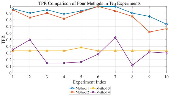
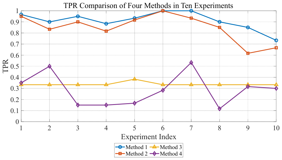
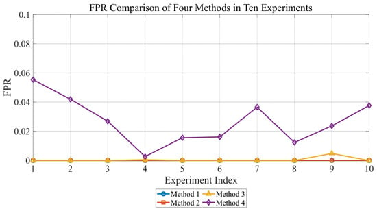
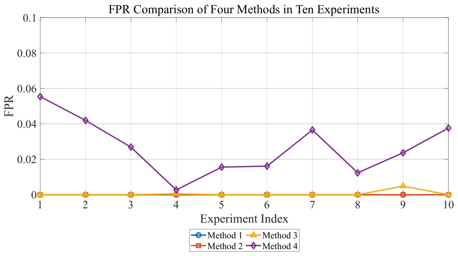
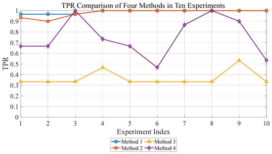
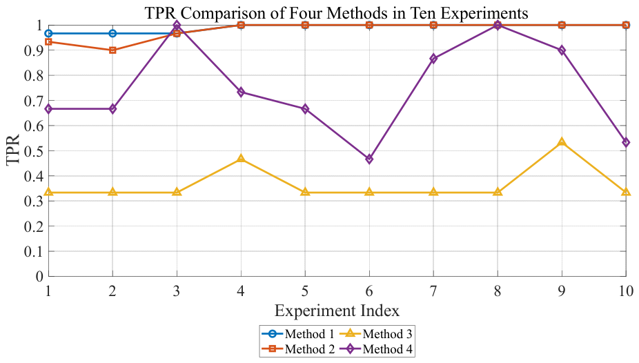
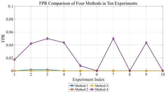
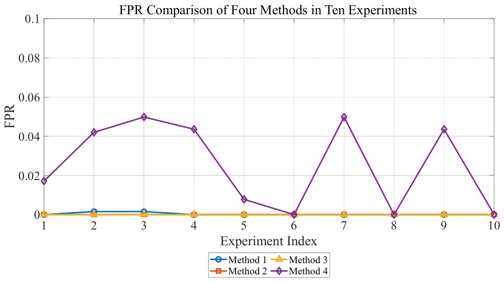
As can be seen from Figure 12, Figure 13, Figure 14 and Figure 15 and Table 8 and Table 9, compared with Methods 2, 3, and 4, the proposed Method 1 not only achieves a higher TPR but also has an FPR comparable to the lowest FPR, indicating that it effectively suppresses false positives while improving the anomaly detection rate. This demonstrates that Method 1 is capable of detecting time snapshots affected by either electricity-theft-induced or communication-anomaly-induced missing events under background disturbances caused by errors and asynchrony. In contrast, the inferior performance of the three comparison methods mainly results from a mismatch between their detection mechanisms and the structural characteristics of severe missing events in LVDNs. Method 2 is primarily designed to distinguish high-leverage observations from regular observations and subsequently identify gross errors through generalized studentized residuals. Although it is robust against leverage effects, masking, and swamping, it focuses mainly on the geometric influence of individual observations and adopts a general residual-based decision criterion, whereas electricity theft and communication anomalies usually cause coordinated changes in the currents of multiple customers and produce a distributed structural mean shift that may not manifest as an isolated bad leverage point. Consequently, its relatively conservative diagnostic mechanism can maintain a low FPR but may fail to identify some abnormal time snapshots. Method 3 relies on labeled historical samples to learn a classification boundary, while its phase-level aggregate and statistical features compress part of the detailed customer-level current relationship. Because abnormal samples are relatively scarce and temporally clustered, and because their characteristics vary with the load level, affected customers, event location, and missing pattern, the learned decision boundary may be biased toward the dominant normal class and may not generalize effectively to unseen anomalies, resulting in a low FPR but a substantially reduced TPR. Method 4 is primarily intended to preserve reliable regression estimates by reducing the influence of contaminated observations and bad leverage points rather than to maximize the detection of every abnormal time snapshot. Its robust fitting process may partially absorb or suppress persistent missing-induced deviations, while a common residual scale and validation-derived decision threshold cannot completely distinguish structural missing events from heterogeneous background disturbances, leading to both missed detections and occasional false alarms. By contrast, Method 1 directly represents each abnormal time snapshot as a possible non-random mean shift in the physically interpretable relationship between the phase-line head-end current and customer-side currents, evaluates its statistical significance while accounting for residual variability and leverage, and controls false discoveries over all phase-time tests. Its detection mechanism is therefore more closely aligned with the actual manifestation of severe missing events, enabling a better balance between TPR and FPR.

Figure 12. TPR of the four methods over 10 experiments in the rural LVDN.

Figure 13. FPR of the four methods over 10 experiments in the rural LVDN.

Figure 14. TPR of the four methods over 10 experiments in the urban LVDN.

Figure 15. FPR of the four methods over 10 experiments in the urban LVDN.

Table 8. TPR and FPR of different methods in the rural LVDN.

Metric Value Method	Method 1	Method 2	Method 3	Method 4
TPR	0.912	0.848	0.338	0.287
FPR	0	0	0.001	0.027

Table 9. TPR and FPR of different methods in the urban LVDN.

Metric Value Method	Method 1	Method 2	Method 3	Method 4
TPR	0.990	0.980	0.367	0.750
FPR	0.001	0	0	0.025

4. Discussion

The proposed method provides a lightweight and physically interpretable data-quality diagnosis tool for LVDNs. By exploiting the regression relationship between the phase-line head-end current and customer-side currents, the mean shift test can detect abnormal time snapshots caused by severe missing-data events without labeled abnormal samples. Therefore, it can be used as a preprocessing module before topology identification, phase identification, state estimation, or other measurement-driven state awareness tasks.

The performance of the proposed method is related to several assumptions. The baseline disturbance model assumes zero-mean Gaussian measurement errors and temporal asynchrony, while practical LVDNs may involve metering bias, clock drift, communication delay, data aggregation effects, and non-Gaussian disturbances. In addition, the regression model uses RMS currents to approximate active current components because most smart meters do not provide synchronized phase-angle information. This approximation is reasonable when customer power factors are relatively high and phase-angle dispersion within the same phase is limited. However, strongly time-varying power factors, large within-phase angle dispersion, extreme phase imbalance, and frequent PV-induced reverse power flow may change the conditional mean relationship used by the test. Therefore, the reported results should not be generalized to these operating conditions without further validation.

In terms of implementation, the main computational burden of the proposed method comes from least-squares regression and residual-based mean shift testing. Since no supervised training or large-scale hyperparameter tuning is required, the method is computationally lightweight and suitable for offline batch screening or periodic data-quality diagnosis in transformer areas. For real smart-meter datasets, preprocessing steps such as time-stamp alignment, meter calibration, missing-value handling, and communication-delay checking are necessary to ensure reliable current regression modeling.

The residual diagnostics indicate that the classical regression assumptions are not satisfied exactly in all phase-specific cases; therefore, the theoretical F-test p-values should be interpreted as nominal statistical indicators. Although no substantial false-positive inflation is observed in the considered simulations, robust covariance correction or block-resampling calibration may be required for field smart-meter data with stronger autocorrelation or heteroscedasticity.

The proposed method still has several limitations. The current evaluation mainly focuses on abnormal time-section detection and cannot independently identify the exact affected customers or determine the definitive physical causes of anomalies. When multiple missing-data mechanisms occur simultaneously, their effects may be coupled in the regression residuals. Although both rural and urban LVDN scenarios are considered in this study, the sensitivity of the proposed method to network scale, distributed PV penetration, and combined disturbances, broader field-calibrated disturbance ranges, and interactions between disturbance types can be further investigated. Future work will further investigate customer-level localization, anomaly cause classification, integration with topology identification, and validation using field smart-meter data. Although the general missing-rate formulation includes file omission, the detection performance reported in this study is validated only for electricity-theft-induced and communication-anomaly-induced severe missing events. File-omission scenarios remain to be investigated in future work.

5. Conclusions

This paper focuses on detecting time snapshots affected by severe missing events under the condition that errors and asynchrony are modeled as background disturbances. First, a unified mathematical model comprising the error rate, asynchrony rate, and missing rate is established to characterize three typical types of gray data: errors, asynchrony, and missing. Second, a phase-specific current regression model for severe missing-event detection is constructed by exploiting the multiple linear regression relationship between the phase-line head-end current and the customer-side currents. Furthermore, a statistical identification method based on the mean shift test is proposed, which converts the detection of time snapshots into a hypothesis testing problem, thereby enabling effective identification of severe missing events.

Simulation results from the ten temporally relocated comparative trials show that the proposed method achieves an average TPR of 0.912 and an average FPR of 0 in the rural LVDN, and an average TPR of 0.990 and an average FPR of 0.001 in the urban LVDN. Compared with the leverage-based, supervised-learning, and robust-regression methods, the proposed method achieves a higher TPR while maintaining a comparably low FPR, thereby providing the best overall TPR–FPR trade-off in the considered cases.

References

- Yi, Y.; Liu, S.; Zhang, Y.; Xue, Y.; Deng, W.; Li, Q. Phase Identification of Low-voltage Distribution Network Based on Stepwise Regression Method. J. Mod. Power Syst. Clean Energy 2023, 11, 1224–1234. [Google Scholar] [CrossRef] [Scilit]
- Afrasiabi, S.; Allahmoradi, S.; Liang, X. Pseudo-Measurement Models in Distribution Networks: A Review. IET Smart Energy Syst. 2025, 1, 56–72. [Google Scholar] [CrossRef] [Scilit]
- Yu, X.; Jiang, R.; Jin, X.; Jia, H.; Mu, Y.; Wei, W.; Tang, W. Method for compensating multi-time measurement data of distribution network based on alternating minimization matrix completion combined with VMD-ARIMA-LSTM. Energy AI 2025, 21, 100563. [Google Scholar] [CrossRef] [Scilit]
- Fang, J.; Zheng, L.; Liu, C. A Novel Method for Missing Data Reconstruction in Smart Grid Using Generative Adversarial Networks. IEEE Trans. Ind. Inform. 2024, 20, 4408–4417. [Google Scholar] [CrossRef] [Scilit]
- Madsen, A.L.; Bhattacharya, S.; Jensen, C.D.; Olsen, R.L.; Schwefel, H.-P. Wrong Data Detection in Electricity Distribution Grids Using Bayesian Networks. In Symbolic and Quantitative Approaches to Reasoning with Uncertainty; Springer: Cham, Switzerland, 2025; Volume 16099, pp. 31–45. [Google Scholar] [CrossRef] [Scilit]
- Rajasekaran, J.R.K.; Natarajan, B.; Jiang, J. Online Bad Data Detection in Compressed Sensing-Based Distribution System State Estimation. IEEE Trans. Smart Grid 2025, 16, 3449–3452. [Google Scholar] [CrossRef] [Scilit]
- Hu, J.; Hu, W.; Cao, D.; Chen, J.; Abulanwar, S.; Hassan, M.K.; Chen, Z.; Blaabjerg, F. Robust Distribution System State Estimation Considering Anomalous Real-Time Measurements and Topology Change. J. Mod. Power Syst. Clean Energy 2025, 13, 928–939. [Google Scholar] [CrossRef] [Scilit]
- Khan, S.; Aboushady, A.A.; Nazir, F.U.; Farrag, M.E. Fault detection and localization in LV distribution networks using anomaly detection in smart meter data and distribution network digital twin. IEEE Access 2026, 14, 17525–17539. [Google Scholar] [CrossRef] [Scilit]
- Rolim, F.B.B.; Trindade, F.C.L.; Cunha, V.C. Composite Index for Identifying Anomalies in Low Voltage Systems Using Smart Meter Measurement Data. IEEE Open Access J. Power Energy 2025, 12, 306–317. [Google Scholar] [CrossRef] [Scilit]
- Zhang, H.; Liu, B.; Wu, H. Smart Inverter Enabled Meter Encoding for Detecting False Data Injection Attacks in Distribution System State Estimation. J. Mod. Power Syst. Clean Energy 2025, 13, 1776–1786. [Google Scholar] [CrossRef] [Scilit]
- Liao, X.; Cui, W.; Zhang, M.; Zhang, A.; Hu, P. Optimized Two-Stage Anomaly Detection and Recovery in Smart Grid Data Using Enhanced DeBERTa-v3 Verification System. Sensors 2025, 25, 4208. [Google Scholar] [CrossRef] [Scilit]
- Takiddin, A.; Ismail, M.; Zafar, U.; Serpedin, E. Deep Autoencoder-Based Anomaly Detection of Electricity Theft Cyberattacks in Smart Grids. IEEE Syst. J. 2022, 16, 4106–4117. [Google Scholar] [CrossRef] [Scilit]
- Lepolesa, L.J.; Achari, S.; Cheng, L. Electricity Theft Detection in Smart Grids Based on Deep Neural Network. IEEE Access 2022, 10, 39638–39655. [Google Scholar] [CrossRef] [Scilit]
- Huang, L.; Wang, M.; Wang, L.; Cao, J. A Missing Data Imputation Method for Distribution Network Data Based on TGAN-GP. Energies 2026, 19, 30. [Google Scholar] [CrossRef] [Scilit]
- Cheng, Y.; Foggo, B.; Yamashita, K.; Yu, N. Missing Value Replacement for PMU Data via Deep Learning Model with Magnitude Trend Decoupling. IEEE Access 2023, 11, 27450–27461. [Google Scholar] [CrossRef] [Scilit]
- Chen, L.; Feng, G.; Wang, L. A Novel Gating Adversarial Imputation Method for High-Fidelity Restoration of Missing Electrical Disturbance Data. Electronics 2025, 14, 4108. [Google Scholar] [CrossRef] [Scilit]
- Pan, J.; Yu, B.; Yu, T.; Gui, X. Monitoring data of substation equipment based on stack-type noise reduction self-encoder hybrid cleaning framework. Electr. Power Syst. Res. 2026, 253, 112518. [Google Scholar] [CrossRef] [Scilit]
- Ren, C.; Xu, Y. A Fully Data-Driven Method Based on Generative Adversarial Networks for Power System Dynamic Security Assessment with Missing Data. IEEE Trans. Power Syst. 2019, 34, 5044–5052. [Google Scholar] [CrossRef] [Scilit]
- Zhang, Y.; Yi, Y.; Deng, W.; Liu, S.; Zhou, L.; Lin, K.; Cai, Y. Consumer-branch Connectivity Identification of Low Voltage Distribution Networks Based on Data-Driven Approach. Prot. Control Mod. Power Syst. 2024, 9, 69–82. [Google Scholar] [CrossRef] [Scilit]
- Zhou, L.; Li, Q.; Zhang, Y.; Chen, J.; Yi, Y.; Liu, S. Consumer phase identification under incomplete data condition with dimensional calibration. Int. J. Electr. Power Energy Syst. 2021, 129, 106851. [Google Scholar] [CrossRef] [Scilit]
- Liu, S.; Deng, C.; Zheng, Z.; Zhu, Y.; Lu, H.; Liu, W. Confidence-aware Topology Identification in Low-voltage Distribution Networks: A Multi-source Fusion Method Based on Weakly Supervised Learning. Energies 2026, 19, 1503. [Google Scholar] [CrossRef] [Scilit]
- Pappu, S.J.; Bhatt, N.; Pasumarthy, R.; Rajeswaran, A. Identifying Topology of Low Voltage Distribution Networks Based on Smart Meter Data. IEEE Trans. Smart Grid 2018, 9, 5113–5122. [Google Scholar] [CrossRef] [Scilit]
- Prostejovsky, A.M.; Gehrke, O.; Kosek, A.M.; Strasser, T.; Bindner, H.W. Distribution Line Parameter Estimation Under Consideration of Measurement Tolerances. IEEE Trans. Ind. Inform. 2016, 12, 726–735. [Google Scholar] [CrossRef] [Scilit]
- Majumdar, A.; Pal, B.C. Bad Data Detection in the Context of Leverage Point Attacks in Modern Power Networks. IEEE Trans. Smart Grid 2018, 9, 2042–2054. [Google Scholar] [CrossRef] [Scilit]
- Mohajon, R.; Sarker, S.C.; Abid, M.A.S.; Ronobir, S.D.; Rumi, A.K.; Chakraborty, S.; Juoairia, A.; Mohammad, N. A Physics-Guided Explainable Machine Learning Framework for Residual-Based Performance Deviation Detection and Probabilistic Severity Assessment in Photovoltaic Systems. Clean Energy 2026, 10, 143–163. [Google Scholar] [CrossRef] [Scilit]
- Miles, A.G.; Chakhchoukh, Y.; Alam, S.M.S. Robust Distribution State Estimation for Reliable Locational Marginal Pricing Under Cyber-Attacks. IEEE Trans. Power Syst. 2024, 39, 4963–4974. [Google Scholar] [CrossRef] [Scilit]
Disclaimer/Publisher’s Note: The statements, opinions and data contained in all publications are solely those of the individual author(s) and contributor(s) and not of MDPI and/or the editor(s). MDPI and/or the editor(s) disclaim responsibility for any injury to people or property resulting from any ideas, methods, instructions or products referred to in the content. |
© 2026 by the authors. Licensee MDPI, Basel, Switzerland. This article is an open access article distributed under the terms and conditions of the Creative Commons Attribution (CC BY) license.