


Abstract
Permeability prediction and hydraulic rock typing in carbonate reservoirs remain challenging because similar porosity values may correspond to markedly different flow capacities controlled by pore throat size, connectivity, and capillary accessibility. This study aims to develop an integrated workflow for permeability prediction and petrophysical–hydraulic rock typing of a heterogeneous dolomite reservoir using parameters that directly characterize the drainable pore throat network. Routine core analysis, centrifuge-derived capillary pressure curves, nuclear magnetic resonance spectra, electrical measurements, petrographic and SEM observations, and fractal descriptors were jointly analyzed. Capillary pressure curves were fitted with the Li–Horne model and transformed into equivalent pore throat radius distributions; characteristic radii , Swanson and Capillary-Parachor parameters, irreducible water saturation, and fractal characteristics were calculated for subsequent regression analysis and rock typing. The conventional relationship showed limited predictive capability, whereas models incorporating provided a more reliable permeability estimate. The best-performing relationship was close to , supporting the interpretation of as a centrifuge-derived analog of the effective hydraulic radius. Comparison with FZI, Winland R35, NMR groups, and electrofacies showed that -based typing produced a compact separation of samples by hydraulic quality. The proposed workflow is presented as a single-well proof of concept and requires validation in independent wells before application to field-scale geological and hydrodynamic models.
1. Introduction
In carbonate reservoirs, permeability and flow behavior are governed by pore systems operating across multiple scales, from micropores and intercrystalline pore networks to vugs, fractures, and zones of secondary mineral cementation [1,2]. Consequently, rocks with similar connected porosity may exhibit fundamentally different permeability values [3,4]. In reservoir simulation, this uncertainty directly affects simulated flow paths, estimates of well productivity and injectivity, fluid transition zones, and the selection of relative permeability and capillary pressure functions [5,6,7]. At the field development scale, pore network heterogeneity controls not only effective flow capacity but also the distribution and trapping of residual fluids after waterflooding [8,9]. Reservoir permeability may also evolve when the pore fracture network is subjected to thermo-mechanical loading [10,11].
The evolution of permeability prediction models reflects a gradual transition from simple relationships to descriptors directly related to the geometry and conductivity of the pore network. In the Kozeny–Carman and Purcell–Burdine models, the rock is considered a system of capillary channels in which permeability is related to porosity, specific surface area, hydraulic radius, and the shape of the capillary pressure curve [12,13,14]. The Timur and Coates models emphasized the role of irreducible water saturation and the movable fluid fraction, thereby shifting the focus from total pore volume to the flow-effective pore volume [15,16,17]. A further step was associated with the use of mercury injection capillary pressure (MICP) data: Winland, Swanson, and Pittman showed that permeability is often better described not by porosity alone but by a characteristic pore throat radius or by a characteristic point on the capillary pressure curve [18,19,20].
One of the most widely used approaches to radius-based permeability interpretation is Winland R35, which relates porosity and permeability to the pore throat radius at 35% mercury saturation. The Swanson and Pittman relationships are based on a similar physical concept, in which permeability is correlated with capillary pressure curve parameters reflecting the contribution of the most conductive part of the pore space [21]. However, these relationships were calibrated mainly using MICP data. Therefore, their published coefficients cannot be directly transferred to centrifuge-derived gas–water capillary pressure curves without additional verification because the fluid pair, wetting state, pressure range, saturation definition, and accessible pore throat domain are different [22].
Capillary pressure curves are among the most informative sources of parameters describing the drainable part of the pore space [23]. Centrifuge capillary pressure measurements make it possible to obtain capillary pressure curves on core samples using a gas–water fluid pair, which is closer to the displacement conditions considered in this study than mercury–air MICP measurements [24,25]. Since the experiment provides discrete values of average water saturation at specified capillary pressure steps, a continuous capillary pressure–water saturation relationship, , must be reconstructed to calculate derived parameters [26]. Compared with MICP curves, centrifuge measurements contain substantially fewer pressure saturation points and therefore cannot provide a unique non-parametric pore size distribution without an explicit approximation model. In this study, both the Brooks–Corey and Li–Horne models were evaluated. The Li–Horne model was retained for the principal radius calculations because its finite upper pressure bound enables reconstruction of the bounded radius distribution required for calculating , whereas Brooks–Corey was retained as a parsimonious reference model. Based on the fitted curves, equivalent pore throat radius distributions, volume-weighted radii, and Swanson and Capillary-Parachor parameters were calculated from centrifuge-derived capillary pressure data [27,28].
Classical reservoir rock typing addresses the same problem from another perspective by grouping samples into classes with similar flow behaviors [29]. In this context, the Reservoir Quality Index (RQI) and Flow Zone Indicator (FZI), which are based on the modified Kozeny–Carman equation and the concept of the mean hydraulic radius, are widely used [30,31]. These indices are useful for identifying hydraulic flow units; however, in complex carbonate rocks, they should be supplemented by directly measured or independently interpreted parameters that capture capillary behavior, electrical response, and pore size distribution [32].
Nuclear magnetic resonance (NMR) provides an additional source of information on pore structure organization [33]. NMR spectra allow the pore volume to be divided into bound and movable components, and they make it possible to estimate the logarithmic mean relaxation time, the position of the dominant peak, and the contribution of different pore space domains [34]. When combined with centrifuge-derived capillary pressure data, NMR measurements can be used to convert distributions into effective radii through the coefficient , providing a basis for a calibrated comparison between the fluid-filled pore body distribution and the drainage-accessible pore throat distribution [35].
Electrical properties complement this workflow because Archie parameters respond to pore network geometry, tortuosity, and the fraction of the connected conductive phase [36]. For heterogeneous carbonates, single values of the cementation exponent and tortuosity coefficient do not always adequately describe the entire dataset [4]. A more appropriate approach is to determine these parameters within electrofacies or petrophysically homogeneous rock types. Such a comparison is particularly important when transferring core-based rock typing to well-log interpretation and geological modeling [37]. In the present study, the electrical parameters are therefore used primarily as supporting descriptors of conductive connectivity and preparation-state differences rather than as independent permeability predictors.
Fractal parameters are considered an additional quantitative tool for describing pore structure complexity [38,39]. Fractal dimensions calculated from capillary pressure curves, NMR spectra, and SEM/thin-section images are not interchangeable [3,7,40]. Capillary pressure measurements characterize pore throats accessed during drainage and water retention behavior, NMR reflects the distribution of fluid-filled pore volume, and image analysis describes the two-dimensional morphology of visible pore space. Therefore, fractal descriptors are used not as a standalone universal permeability model but as structural constraints for interpreting radius-based permeability models and rock typing [41,42]. Only physically admissible and non-redundant fractal descriptors with a clear relationship to permeability, irreducible water saturation, or NMR pore space groups are retained in the principal interpretation.
The objective of this study is to determine whether characteristic radii derived directly from gas–water centrifuge drainage curves can improve permeability prediction and provide an independent capillary basis for hydraulic rock typing in a heterogeneous dolostone interval. To achieve this objective, capillary pressure curves were fitted with the Li–Horne model; characteristic radii and Swanson and Capillary-Parachor parameters were calculated; relaxation times were converted into effective radii; capillary, NMR, fractal, and electrical parameters were compared; and regression models for permeability prediction were constructed. The main hypothesis of this study is that, for the investigated carbonates, permeability is controlled not by total porosity but by the size and connectivity of the drainable part of the pore space. Therefore, radius-based descriptors are expected to provide a more robust prediction than the basic relationship.
Existing characteristic-radius permeability relationships are predominantly derived from mercury–air intrusion data or are back-calculated from measured permeability and porosity. Their empirical coefficients cannot be directly transferred to gas–water centrifuge curves because the fluid pair, pressure range, saturation definition, and accessible pore throat domain differ. In addition, NMR primarily characterizes fluid-filled pore bodies, whereas drainage capillary pressure is controlled mainly by accessible pore throats; therefore, direct comparison of the two distributions requires explicit calibration. Accordingly, the direct capillary-derived radius is distinguished throughout this study from the inverse routine-core proxy . The direct radius is used for permeability model development on the matched centrifuge subset, whereas is used only to propagate the calibrated hydraulic ordering to the broader routine-core dataset. Because all investigated samples originate from a single well, the resulting relationships are considered section-specific and require validation in independent wells before field-scale application.
2. Materials and Methods
2.1. Core Material and Initial Data
The study used standard cylindrical carbonate core plugs obtained from a single well in the Mirny District of the Republic of Sakha (Yakutia), Russia. The physical core interval of 1751.0–1775.0 m corresponds to 1752.4–1776.4 m on the log-matched depth scale and encompasses the Upper and Lower Bilir units of the Osinsky horizon. The interval consists predominantly of dolostones and includes dense, porous, and porous–vuggy lithotypes, thereby capturing pronounced within-well lithological and petrophysical heterogeneity. However, because all samples were obtained from a single well, the collection cannot independently characterize field-scale spatial variability.
Before plug sampling, the full-diameter core was reconstructed, depth-marked, and continuously profiled using spectral gamma-ray and density scanning. Surface gas permeability was measured with a laboratory-built, non-commercial probe permeameter at an average spacing of approximately 3 cm. The core gamma-ray response was matched to the corresponding well logs, and plug locations were purposefully selected using the resulting depth, density, permeability, and lithological profiles. Thus, sampling was profile-guided rather than random. The plugs were approximately 30 mm in both diameter and length. Because the rocks contained water-soluble salts, water-free cutting and mineral oil cooling were used to minimize halite dissolution.
The initial collection comprised 60 plugs: 30 extracted samples included in the detailed experimental program (1e–30e), 10 non-extracted samples (1n–10n), and 20 samples used only for routine porosity and gas permeability measurements (1k–20k). Samples within each group were numbered in increasing order of core depth. Two plugs were excluded from the baseline porosity–permeability regression because complete paired measurements in the required analysis state were unavailable. Sample 4n was initially tested in the non-extracted state but disintegrated during subsequent extraction, whereas sample 18k split before a reliable absolute gas permeability value could be obtained. Accordingly, 58 samples were retained for the baseline analysis.
Analysis-specific subsets were subsequently selected according to data availability, sample preservation, and measurement quality; missing values were not imputed. Natural fractures, vugs, and mineral-filled discontinuities were retained because they represent the actual heterogeneity of the investigated interval. Gas-measured porosity ranged from 1.4 to 24.2%, absolute gas permeability ranged from 0.02 to 870 mD, and grain density ranged from 2.68 to 2.93 g/cm3. The numbers of samples available and retained at each experimental stage, together with the corresponding quality control criteria, are summarized in Table 1. Extrapolation of the resulting relationships beyond the studied well requires independent external validation.
Table 1.
Data availability, analytical use, and sample exclusion criteria.
The workflow comprised experimental characterization followed by computational interpretation. Routine properties, capillary behavior, NMR, electrical properties, and microstructure were measured on analysis-specific subsets. The computational stage included capillary curve fitting, radius conversion, focused fractal interpretation, rock typing, and permeability model validation. NMR and the inverse routine-core proxy are explicitly recognized as centrifuge-constrained components of the workflow (Figure 1).
Figure 1.
Workflow of the experimental investigation and subsequent data processing and interpretation.
2.2. Routine Petrophysical Measurements
In the first stage, routine measurements of porosity, grain density, and absolute gas permeability were performed on 60 standard core plugs. For the extracted samples, residual hydrocarbons were removed in a Soxhlet apparatus using chloroform for 15–40 h, until the solvent remained visually clear. The plugs were subsequently air-dried at room temperature and then oven-dried to constant mass at 105 °C. Samples containing anhydrite were dried at 80 °C to minimize mineral alteration.
Grain density and skeletal volume were measured using a TPI-219 helium pycnometer (Coretest Systems, Inc., Morgan Hill, CA, USA). Gas-accessible porosity was calculated from the difference between the geometrically determined bulk volume and the helium-measured skeletal volume. The reported uncertainty of the grain density measurements was approximately 1%. Absolute gas permeability was measured with air under steady-state linear-flow conditions using a TBP-804 gas permeameter (Coretest Systems, Inc., Morgan Hill, CA, USA). A pneumatic confining pressure of 1.5 MPa was applied. Measurements were performed at no fewer than three pressure gradients, and absolute permeability was determined by Klinkenberg extrapolation. The estimated uncertainty of the permeability measurements was 4.75%. These measurements were performed under ambient laboratory conditions rather than under reservoir effective-stress conditions; therefore, direct application of the measured permeability values to in situ conditions requires an appropriate stress correction [43].
Two conventional porosity-based permeability relationships were used as baseline models: and , where is absolute gas permeability, mD, and is porosity expressed as a fraction. Both models were fitted and evaluated using the same logarithmic permeability response, , to ensure a consistent comparison of the fitting and predictive errors. Model performance was characterized using the coefficient of determination, leave-one-out cross-validation , and the root mean square error in .
For the electrical measurements, open porosity was additionally determined by saturation with model formation water. The brine density was 1.197 g/cm3. Electrical resistivity was measured on 30 extracted and 10 initially non-extracted plugs using a PetroOm four-electrode impedance meter (EkoGeoSProm, Tver, Russia). The measurements were corrected to 20 °C; the brine resistivity at this temperature was 0.042 Ω⋅m. The reported measurement uncertainties were 5% for the saturated plugs and 0.5% for the brine.
Electrical properties were determined from resistivity measurements on water-saturated samples. The formation resistivity factor was calculated as the ratio of the resistivity of a fully water-saturated sample to the resistivity of the formation water. The relationship between and porosity was described by Archie’s Equation (1) [36]:
where is the electrical resistivity of the fully water-saturated sample, is the electrical resistivity of the formation water, is effective porosity, is the tortuosity factor, and is the cementation exponent. The resistivity index was determined using Equation (2):
where is the electrical resistivity of the sample at the current water saturation, is water saturation, fraction, and is the saturation exponent.
The parameters and were estimated from the relationship, whereas was estimated from the relationship [36,44,45]. Recent studies emphasize that should be regarded not only as a cementation exponent but also as a parameter sensitive to pore space geometry, the tortuosity of electrical current paths, and the fraction of effectively connected conductive porosity. In [46], it is specifically noted that the cementation exponent reflects the electrical connectivity of the conductive phase within the rock.
For carbonate rocks, using a single set of constants , , and for the entire dataset is often insufficiently accurate. These parameters depend on pore space structure, pore network connectivity, pore and pore throat size distribution, fracturing, and diagenetic alteration [45,47]. Therefore, in heterogeneous carbonates, it is more appropriate to determine Archie parameters separately for more homogeneous rock groups rather than to apply one set of coefficients to the entire section [4,44].
2.3. Centrifuge Capillary Pressure Measurements
Capillary pressure measurements were performed using a UTsPF-15000 petrophysical centrifuge (EkoGeoSProm LLC, Tver, Russia). A fully water-saturated core plug was placed in a centrifuge assembly and sequentially subjected to rotational-speed steps corresponding to prescribed capillary pressure values. Each step was maintained for 90–120 min, depending on the petrophysical properties of the plug. After each step, the assembly was removed and weighed, and the average water saturation of the plug was calculated from the change in mass. The applied capillary pressures were 0.05, 0.10, 0.20, 0.40, 0.80, and 1.20 MPa. The rotor speed at each centrifugation step was converted into the corresponding capillary pressure using the Tulbovich equation, which accounts for the density difference between the fluids and the radial positions of the inlet and outlet faces of the core plug. The gravimetric average saturations were fitted directly; no Hassler–Brunner or Forbes inlet face correction was applied. The resulting curves and radii should therefore be interpreted as effective average-saturation descriptors rather than inlet face capillary pressure distributions.
To compare the capillary pressure curves, normalized water saturation was used according to Equation (3):
where is irreducible water saturation, fraction, and is normalized water saturation, fraction.
The experimental curves were described using two models: the Brooks–Corey model and the Li–Horne model. The Brooks–Corey model was used as a baseline approximation (4) [48]:
where is capillary pressure, MPa, is displacement pressure, MPa, and is the Brooks–Corey curve shape parameter.
The main calculations were performed using the Li–Horne model, because it allows the capillary pressure curve to be described while accounting for the upper pressure limit and is related to a fractal representation of pore space (5) [49]:
where is the maximum capillary pressure corresponding to irreducible water saturation, MPa, is the Li–Horne curve shape parameter, and is a constant expressed as follows (6):
For both models, R2, RMSE, and MAE were calculated on water saturation in percentage points. Predictive interpolation was assessed by omitting one pressure step at a time; AICc was also reported because the curves contain only six positive-pressure observations and the models have different parameter counts.
2.4. Radius Distribution
The Young–Laplace equation was used to convert capillary pressure into equivalent pore throat radii (7):
where is the effective pore throat radius, µm, and µm·MPa (a gas–water interfacial tension is the capillary constant, assumed to be the same for the entire calculation series.
The volume-weighted density function of the drainable pore volume with respect to equivalent pore throat radius was then expressed as (8):
Based on this relationship, the volume-weighted mean radius of the drainable domain was calculated using Equation (9), assuming that :
Thus, as decreases, the volume-weighted distribution shifts toward smaller radii, and the mean drainable radius becomes substantially smaller than the maximum radius.
Based on the model parameters, the cumulative fraction of drainable pore volume with radii not exceeding was calculated as (10):
Unlike MICP, which commonly provides a densely sampled pressure–intrusion curve, the centrifuge experiment contained only six pressure steps. Each point is an average equilibrium saturation. Direct differentiation or non-parametric inversion would therefore amplify measurement uncertainty and cannot yield a unique pore throat distribution with MICP-like resolution.
The centrifuge data were consequently interpreted through parametric curves. Brooks–Corey and Li–Horne parameters define finite, model-dependent distributions of equivalent drainable pore throat radii; these distributions are not presented as direct measurements of the complete pore size spectrum.
The characteristic radius was defined as the lower-tail -quantile of the modeled distribution of drainable equivalent pore throat radii, such that . Thus, a fraction of the modeled drainable pore volume is associated with equivalent pore throat radii , whereas the remaining fraction is associated with radii (11):
Here, is a dimensionless cumulative fraction ranging from 0 to 1, while are the lower and upper bounds of the modeled equivalent pore throat radius distribution, respectively. The definition applies only to the drainable pore volume represented by the fitted curve, not to the total pore volume of the rock.
2.5. Swanson and Capillary-Parachor Segmentation Parameters
To characterize the positions of the principal segmentation points, modified centrifuge-based analogs of the Swanson and Capillary-Parachor parameters were calculated [28]. Unlike the original parameters commonly evaluated from densely sampled MICP curves, the present parameters were determined analytically from the continuous fitted Li–Horne curve rather than directly from the six experimental pressure steps. No empirical MICP coefficients were transferred to the centrifuge data. Water saturation was converted to the non-wetting-phase saturation as , with all saturations expressed as fractions.
The Swanson parameter, MPa−1, was defined as the maximum ratio of the involved non-wetting-phase fraction to capillary pressure (12):
The Capillary-Parachor parameter, MPa−2, was defined as the maximum of the following function (13):
These parameters characterize the segment of the capillary pressure curve where the drainable pore volume is accessed most efficiently relative to the applied capillary pressure. After calculating and , regression relationships between permeability and these parameters were constructed both separately and in combination with porosity.
2.6. Nuclear Magnetic Resonance
Nuclear magnetic resonance (NMR) was used as a complementary, centrifuge-constrained method for describing fluid-filled pore bodies and fluid mobility. The relaxation decay of hydrogen-bearing fluid was inverted to an amplitude distribution over transverse relaxation time by treating the problem as a Fredholm integral equation of the first kind and applying Tikhonov regularization [7,34].
NMR measurements were performed on water-saturated plugs using a spectrometer operating at a resonance frequency of 12.5 MHz and a magnetic field strength of approximately 0.29 T. The measurement system and samples were equilibrated at 40 °C. Transverse relaxation decays were recorded using a Carr–Purcell–Meiboom–Gill sequence with a nominal echo spacing of 0.2 ms. The number of echoes was adjusted to record the decay to the noise level, the recovery delay was 22.5 s, and ten signal accumulations were used.
For a water-saturated sample measured at a short echo spacing and in a homogeneous magnetic field, the contributions of bulk and diffusion relaxation are often considered minor compared with surface relaxation. In this case, Equation (14) can be written as follows:
where is the surface relaxivity, is the surface-to-volume ratio of the pore, and is the pore shape geometrical factor; for a cylindrical pore and for a spherical pore. Hence, the effective radius can be expressed as Equation (15):
Neither nor was measured independently. This relationship makes it possible to use the NMR spectrum as a basis for converting the relaxation time distribution into a distribution of effective radii. Therefore, the coefficient was treated as a lumped, sample-specific calibration coefficient rather than as a direct measurement of surface relaxivity. The resulting NMR radii represent an effective pore body scale, whereas the centrifuge-derived radii predominantly characterize hydraulically controlling pore throats.
To convert relaxation time into effective radius for the drainable part of the spectrum, the reverse cumulative curve of movable pore volume was constructed according to Equation (16):
Then, for the same cumulative fraction , the , values obtained from the NMR spectrum were matched with the corresponding values. When a single conversion coefficient was used for an individual sample, it was calculated as the median ratio of radius to the corresponding relaxation time, as shown in Equation (17):
After the relaxation decay was recorded using the Carr–Purcell–Meiboom–Gill (CPMG) sequence, the initial signal was transformed into an amplitude distribution over . The resulting spectra were used to determine total NMR porosity, logarithmic mean relaxation time , the position of the dominant spectral peak , and the fractions of pore volume attributed to bound-fluid, effective-pore, and vuggy-pore components. These parameters were considered descriptors of pore volume distribution and fluid mobility within the pore space.
To separate the spectrum into bound and drainable components, an individual value was determined for each sample using the irreducible water saturation obtained from centrifuge measurements. For each sample, was selected so that the area under the spectrum to the left of the cutoff corresponded to irreducible water saturation, as expressed in Equation (18):
where is the amplitude. This approach makes it possible to reconcile NMR interpretation with centrifuge-derived capillary pressure data: the interval is interpreted predominantly as irreducible or bound water, whereas the interval is assigned to the drainable part of the pore space.
2.7. Fractal Dimensions of the Pore Space
Fractal parameters were retained as complementary multiscale descriptors of pore space heterogeneity rather than as alternative permeability models. Carbonate pore systems contain micropores, intercrystalline channels, dissolution vugs, fracture-related voids, and mineral-filled discontinuities; therefore, a single porosity or mean radius value cannot describe their complete structural organization. Nevertheless, evidence of a power law relationship was evaluated only over the scale interval in which an approximately linear trend was observed in logarithmic coordinates.
Fractal concepts are applied across geoscience at multiple scales, including in the interpretation of nonlinear and unstable evolution in coupled geomechanical systems [50]. For carbonate reservoirs specifically, pore space fractality has been investigated using capillary pressure, NMR, and image-based methods [38,42], while fractal capillary bundle models provide a framework for linking pore geometry to transport behavior [51]. Accordingly, the capillary-, NMR-, and image-derived dimensions used in this study are not treated as interchangeable.
If the pore space exhibits fractal properties, then the cumulative fraction of pore volume with radii smaller than can be expressed by a power law relationship. For the wetting phase, this leads to Equation (19):
where is the fractal dimension calculated from the wetting-phase saturation. The second approach is based on non-wetting-phase saturation and is expressed as Equation (20):
where is a constant and is the fractal dimension calculated from the non-wetting-phase saturation. In [28], it was shown that both wetting-phase-based and non-wetting-phase-based approaches can be used to calculate fractal dimension from MICP curves, and that the curve should preferably be divided into segments according to a characteristic segmentation point.
The NMR-based fractal dimension was determined from the pore volume distribution over transverse relaxation times, . When surface relaxation dominates, is proportional to the effective radius of the pore element; therefore, the cumulative fraction of pore volume can be expressed through . For the cumulative fraction of pore volume with relaxation times shorter than a given value, Equation (21) was used:
where is the cumulative fraction of pore volume, is the maximum relaxation time within the considered interval, and is the fractal dimension derived from NMR data.
The fractal dimension obtained from thin-section and SEM images was calculated as a two-dimensional, or planar, measure of pore space complexity. For this purpose, each image was first segmented into pore and mineral phases, after which the box-counting method was applied. Its general form is given by Equation (22):
where is the number of boxes of size containing elements of the pore space or its boundary, and is the box-counting fractal dimension.
Image-based box counting is sensitive to resolution, segmentation, threshold, and field of view [3,38]. The exploratory analysis initially included dimensions from wetting and non-wetting saturation, complete and partial NMR spectra, and weighted NMR zones. The principal analysis retains only physically admissible, non-redundant descriptors: the structural capillary dimension , the drainable-network dimension , the global NMR dimension , and the tortuosity dimension (Appendix A). Values outside the adopted three-dimensional pore volume range 2 ≤ D ≤ 3 were not used as pore volume dimensions
2.8. Petrophysical and Hydraulic Rock Typing
Several complementary approaches to petrophysical rock typing were used to compare the pore space characteristics of the studied carbonate core material. This comparison is required because carbonate rocks are characterized by pronounced structural and flow heterogeneity; their permeability and capillary properties are controlled not only by the total pore volume but also by pore morphology, pore throat size, connectivity of flow paths, and the nature of diagenetic alteration [52]. Therefore, the methods applied in this study were based on different physical principles: the flow behavior of the pore system, the effective pore throat size, and the structural and textural organization of the carbonate matrix [2,30,53].
The hydraulic flow unit approach proposed in [30] was used as the baseline method. This method is based on the modified Kozeny–Carman equation and assumes that samples characterized by similar mean hydraulic radii and similar flow path geometry should exhibit comparable flow behavior [30,31].
For each sample, the Reservoir Quality Index (RQI) and normalized porosity were calculated using Equations (23) and (24):
where k is permeability, mD. The Flow Zone Indicator (FZI) was then calculated using Equation (25):
It should be noted that the classical RQI/FZI approach is most robust when differences between rock groups are controlled by differences in pore system geometry rather than merely by statistical scatter in porosity–permeability properties. For heterogeneous carbonates, this issue is particularly important because similar porosity and permeability values may correspond to different pore system types and different degrees of flow connectivity [2,54].
The Winland R35 method was also used to characterize the effective pore throat size. This approach assumes that the pore throat radius corresponding to 35% non-wetting-phase saturation in mercury injection tests is one of the most informative parameters linking the flow properties of a rock to its capillary structure [18,20]. In the calculation form, the following relationship was used (26):
For carbonate rocks, the application of R35 is particularly relevant when differences between samples are controlled by the development of intercrystalline and vuggy pore systems. However, R35 should be regarded as an empirical indicator, and its interpretation should be performed together with other rock-typing methods rather than in isolation [20,55].
2.9. Statistical Analysis and Model Validation
All permeability regressions were fitted in the domain. Model performance was assessed using the calibration coefficient of determination , leave-one-out cross-validated coefficient , , and . In each iteration, one sample was excluded, the model coefficients were recalibrated using the remaining samples, and permeability was predicted for the excluded sample.
Because q and several functional forms were screened, nested repeated the complete selection procedure within each training fold. In addition, 10,000 bootstrap samples were drawn with replacement; , coefficients, , and were re-estimated in every realization. Predictor influence was assessed from leverage, studentized residuals, Cook’s distance, DFFITS, and leave-one-sample coefficient changes. Influential samples were retained when physically valid, and sensitivity variants were reported rather than used for automatic deletion. Calculations, statistical analyses, data processing, and visualization were performed using Python 3.14.7 and Microsoft Excel 2019, including custom Python scripts developed for this study.
3. Results
3.1. Petrophysical Properties of the Studied Carbonate Core Samples
The 58 paired routine measurements span several orders of magnitude in permeability. The porosity-only exponential and power law baselines gave and 1, respectively (Figure 2), confirming that porosity alone does not resolve the contrasting connectivity of the studied pore systems.
Figure 2.
Relationship between absolute gas permeability and porosity: (a) exponential relationship; (b) power-law relationship. Blue dots represent the measured core-plug data, and orange lines represent the fitted regression models.
Both capillary models reproduced the measured average saturations, but their statistical strengths differed. Li–Horne gave lower in-sample RMSE for all 39 matched curves and lower omitted-pressure-step RMSE, whereas AICc favored the more parsimonious Brooks–Corey model for all samples because only six positive-pressure observations were available (Table 2).
Table 2.
Comparison of Brooks–Corey and Li–Horne models.
Li–Horne was retained for finite-range interpolation and bounded Rq reconstruction, while Brooks–Corey was retained as the parsimonious reference. Thus, Li–Horne was selected for the intended radius calculation, not claimed to be universally superior. Summary statistics for the 39 matched samples are reported in Table 3.
Table 3.
Summary statistics of the parameters of the 39 carbonate core samples.
The observed differences are clearly reflected in the shapes of the capillary pressure curves. Some samples are characterized by low entry pressures and a rapid decrease in water saturation at low capillary pressure values, indicating the presence of relatively large and well-connected drainable channels. In contrast, other samples require higher capillary pressures to involve the pore space in drainage; such curves are usually associated with increased irreducible water saturation, smaller effective pore throat radii, and more pronounced microporosity.
The mineralogical composition of the studied samples is dominated by dolomite, which accounts for 90–99.6% in most samples, with a maximum of 99.6% in sample 5e and a minimum of 77.4% in sample 26e. This indicates the predominance of a dolomitized carbonate matrix and only a minor siliciclastic admixture. The silicate fraction is generally low: quartz varies from 0.3 to 5.2%, with elevated values observed in samples 20e–21e, whereas microcline is absent in most samples or occurs only in trace amounts, reaching 2.2% in sample 20e. Evaporite minerals show more pronounced variability: halite is usually absent but locally increases to 6.9–8.7% in samples 13e, 1n, and 6n, whereas anhydrite is commonly absent but increases to 4.8–6.0% in samples 20e and 27e and reaches 20.1% in sample 26e, reflecting episodes of enhanced sulfate mineralization. Calcite occurs in minor amounts, generally below 1%, with a maximum of 1.8% in sample 21e, indicating that the calcite phase plays a subordinate role relative to dolomite. Overall, the distribution of accessory minerals emphasizes lithological and probably facies-diagenetic heterogeneity within a generally dolostone-dominated rock assemblage.
Anhydrite, halite, and fine-grained impurities affect hydraulic interpretation and may promote fines migration during aqueous treatment [56,57]. Halite dissolution during brine saturation can also alter mass, connected porosity, and local pore geometry; it is therefore a possible source of coupled uncertainty in the electrical, NMR, and centrifuge measurements.
Extraction increased porosity and permeability in all paired samples. The median porosity increase was 3.69 percentage points, while the median permeability increase was 0.70 mD. The median permeability ratio was 2.08, and the geometric mean ratio was 3.43. Salt removal also increased both properties in all samples, with median increases of 1.14 percentage points in porosity and 3.28 mD in permeability. The median permeability ratio was 1.23, whereas the geometric mean ratio reached 4.65 because samples 2n and 6n showed exceptionally large responses. For both treatments, the paired increases in porosity and permeability were significant according to the exact Wilcoxon signed-rank test (W = 0, p = 0.0039).
During salt removal, mass loss was strongly correlated with the increases in porosity ( = 0.917, p = 0.0005) and absolute permeability ( = 0.817, p = 0.0072). For the seven plugs with XRD data, initial halite content was positively correlated with both mass loss and porosity increase ( = 0.852, p = 0.0148). Its relationship with permeability increase was also positive but statistically uncertain ( = 0.704, p = 0.077). These results indicate that soluble pore-filling material locally restricted accessible pore volume, whereas permeability increased substantially only where newly opened voids formed connected flow paths. Because only nine paired samples and seven mineralogically characterized samples were available, these correlations should be regarded as exploratory.
Consistent with these preparation-induced changes, Archie parameters differed between the extracted and non-extracted subsets. The extracted samples yielded a = 2.36, m = 1.67, and n = 1.55, whereas the non-extracted samples yielded a = 4.53, m = 1.43, and n = 1.84. Cluster bootstrap analysis confirmed a systematically higher saturation exponent in the non-extracted subset, with a 95% interval of 0.215–0.437 for the between-group difference. The higher n indicates a stronger resistivity increase during desaturation, likely reflecting residual hydrocarbons or salts and reduced continuity of the conductive water phase.
Published carbonate datasets show that Archie parameters vary widely with pore structure. The obtained m values fall within reported carbonate ranges, while the extracted-sample n = 1.55 is consistent with a strongly connected or preparation-modified pore system and the non-extracted value n = 1.84 approaches typical water-wet carbonate values. The relatively high fitted a values should not be interpreted as direct measures of tortuosity because a and m are covariant regression parameters and are sensitive to the porosity range, electrical facies, and high formation factors of low-porosity samples. Accordingly, separate Archie equations were retained for the extracted and non-extracted subsets, whereas the combined equation was treated only as an average empirical relationship for the Osinsky collection.
To illustrate differences in pore space architecture, three representative samples were selected: 2e, 21e, and 10n (Figure 3). These samples represent different variants of microstructural organization in the carbonate core material and are used as reference examples for interpreting capillary, NMR, and microstructural parameters.
Figure 3.
Thin sections and SEM images of representative samples: (a) 2e—porous–vuggy dolostone; (b) 21e—tight microporous dolostone with a mineralized fracture; (c) 10n—intercrystalline-pore dolostone.
Thin-section and SEM image analysis showed that the studied carbonate samples differ in the degree of recrystallization, pore space type, and scale of pore heterogeneity. The main diagnostic features used for rock typing are visible porosity in thin sections, pore distribution pattern, the presence of vugs and intercrystalline channels, the fractal dimension of the pore space boundary, and SEM-derived microporosity parameters.
Samples 2e and 10n have almost identical segmented pore area fractions, 13.20% and 13.12%, respectively, but differ markedly in pore connectivity. In sample 2e, the largest connected pore–vug cluster accounts for 24.23% of the segmented pore area, compared with only 6.81% in sample 10n. Sample 21e contains only 5.33% visible pore area and has the smallest connected cluster, 1.55% (Table 4).
Table 4.
Quantitative thin-section pore space descriptors for the representative samples.
These results quantitatively support the interpretation of sample 2e as a connected pore–vug system, sample 10n as a more fragmented intercrystalline system, and sample 21e as a tight microporous end member.
Comparison of the three samples indicates that at least three characteristic types of pore space organization occur in the studied section:
- a secondarily altered pore–vug fracture type, in which permeability is controlled by the connectivity of secondary voids;
- a relatively uniform intercrystalline-pore type forming the matrix reservoir;
- a structurally complicated intercrystalline-pore type, in which flow is restricted by narrow channels, pore compartmentalization, and partial mineral filling of the pore space.
Thus, routine petrophysical measurements, mineralogical analysis, thin sections, and SEM observations show that the studied collection cannot be described by a single general relationship. Further permeability prediction therefore requires parameters that characterize the drainable part of the pore space, including capillary pressure curve shape, irreducible water saturation, equivalent pore throat radii, and drainage segmentation parameters.
3.2. Capillary Pressure Curves and Radius Distribution
To quantitatively characterize the drainable part of the pore space, the fitted parameters of the Li–Horne model were converted into distributions of equivalent pore throat radii. Figure 4 shows the equivalent-radius distributions for the complete sample set and for the three representative samples, 2e, 21e, and 10n.
Figure 4.
Equivalent pore throat radius distributions derived from centrifuge capillary pressure data: (a) complete sample set; (b) samples 2e, 21e, and 10n.
The distributions confirm the microstructural differences between the representative samples. Sample 2e shows a shift in the drainable pore volume toward larger radii, which is consistent with its porous–vuggy fabric and high permeability. Sample 21e is concentrated mainly in the fine- and medium-radius intervals, reflecting higher capillary resistance and low permeability. Sample 10n occupies an intermediate position and is characterized by a more heterogeneous distribution, which is consistent with an intercrystalline, matrix-dominated pore system.
Thus, the equivalent-radius distribution calculated from centrifuge-derived capillary pressure data provides a quantitative description of the differences previously identified from thin-section and SEM observations. This makes it possible to relate microstructural heterogeneity to parameters that are directly suitable for subsequent correlation analysis of permeability.
3.3. Segmentation Points of Capillary Pressure Curves and Characteristic Radii Rq
The next stage of the analysis was the determination of capillary curve segmentation parameters. While the characteristic radii define the position of a specified cumulative fraction of the drainable pore volume on the radius scale, the Swanson and Capillary-Parachor parameters identify the part of the capillary pressure curve where pore space involvement in drainage is most efficient relative to the required capillary pressure.
For each fitted curve, the non-wetting-phase saturation was calculated, after which the maxima of the corresponding functions were determined. The resulting points were interpreted as centrifuge-based analogs of the Swanson and Capillary-Parachor parameters, which have previously been applied mainly to MICP data. This approach avoids the direct transfer of MICP correlation coefficients and allows segmentation characteristics to be calculated directly from centrifuge-derived capillary pressure data, even when the number of experimental points is limited.
The positions of the segmentation points differ among samples with different pore space types. In samples with large and well-connected pore throats, the function maxima are reached at lower pressures and at larger fractions of the accessed pore volume. In tight microporous samples, the segmentation points shift toward higher pressures and smaller effective radii, reflecting the need for higher capillary pressure to involve the pore system in drainage. Table 5 presents the calculated Swanson and Capillary-Parachor segmentation parameters for samples 2e, 21e, and 10n.
Table 5.
Segmentation points for samples 2e, 21e, and 10n.
The physical meaning of the parameter is that it estimates the ratio between the fraction of the accessed drainable pore volume and the capillary pressure required for displacement. A higher value of this parameter indicates that a larger part of the pore space is involved in drainage at lower pressure, which usually corresponds to larger and better-connected pore throats. The parameter additionally amplifies the pressure contribution through the squared denominator and is therefore more sensitive to the early stage of drainage and the entry capillary pressure. The obtained permeability relationships based on the Swanson and Capillary-Parachor parameters are presented in Table 6.
Table 6.
Permeability relationships based on segmentation points and porosity (fraction).
Including porosity substantially improves the quality of both the Swanson- and Capillary-Parachor-based models. However, even the porosity-modified Capillary-Parachor relationship is inferior to the models based on characteristic radii. This indicates that, for the studied dataset, the most informative parameters are not the maxima and , but rather the radius corresponding to a specified fraction of the drainable pore volume. Figure 5 presents the results of testing based models for different fractions of the drainable pore volume. A substantially larger number of models was examined in this study.
Figure 5.
Stability of characteristic-radius selection: (a) LOOCV across q; (b) distribution of q selected in 10,000 bootstrap resamples. In panel (b), the green shaded band denotes the interquartile range of the bootstrap-selected q values (15–21%), and the red dashed line denotes the median value (18%).
The maximum LOOCV was obtained for R17 ( = 0.9494), but the response was broad: R15–R21 remained within 0.001 of the maximum. In 10,000 bootstrap resamples with reselected in each realization, the median selected q was 18%, the interquartile range was 15–21%, and the 95% percentile interval was 11–31%. Nested LOOCV, in which was reselected after excluding each sample, gave = 0.9462, RMSE = 0.2593 log10 (mD), MAE = 0.2170 log10 (mD), and a measured–predicted slope of 0.995. Therefore, R20 was retained as a convenient and physically interpretable representative of a stable early-drainable interval, rather than as a unique optimum or a universal carbonate constant.
Table 7 reports the two retained characteristic-radius models. The optimum was not a unique quantile: formed a stable plateau. These radii characterize the stable lower-quantile interval of the modeled drainable pore throat radius distribution. was retained as a convenient representative of this formation-specific plateau.
Table 7.
Permeability relationships based on
The obtained results are consistent with the general logic of radius-based MICP models, including Winland R35, in which permeability is related to a characteristic pore throat radius.
The Kozeny–Carman equation can be rewritten in terms of the hydraulic radius as . The centrifuge-derived is not strictly identical to the classical hydraulic radius because it represents a quantile of the drainable pore throat distribution. Assuming that , the Kozeny–Carman relationship becomes . For a circular-equivalent pore throat, , giving . Therefore, the proposed relationship can be regarded as a generalized Kozeny–Carman-type model. For the fitted exponent was B = 1.0702, whereas fixing B = 1 resulted in only a minor reduction in model performance. The fixed-exponent coefficient corresponds to = 5.825 and = 1.707, supporting the physical plausibility of as a characteristic flow-controlling pore throat scale.
3.4. NMR Descriptors, Sample Grouping, and Permeability Models
Unlike centrifuge measurements, which primarily characterize drainable pore throats, NMR describes the distribution of hydrogen-bearing fluid over transverse relaxation times, . Direct comparison therefore requires the sample-specific, centrifuge-constrained conversion described in Section 2.6.
The obtained values range from 8.44 to 42.09 ms, with a median value of 31.34 ms. This variation confirms that a single universal value for the entire section does not capture differences in pore structure.
The coefficient was recalculated by matching the NMR distribution with the Li–Horne radius distribution. The median value for the samples is approximately 0.016 µm/ms, with a range from 0.0026 to 0.0406 µm/ms. Therefore, is not merely a conversion coefficient but also a rock-typing parameter that links relaxation-based and capillary descriptors.
NMR grouping based on the fractions of three pore space zones divided the samples into three groups (Table 8). Zone 1 corresponds to T2 ≤ 35 ms, Zone 2 to 35 < T2 ≤ 750 ms, and Zone 3 to T2 > 750 ms.
Table 8.
Summary parameters of the NMR groups of the studied samples.
Joint analysis of the distributions and effective-radius distributions shows that the studied dataset includes several pore space types: microporous samples dominated by short components and small radii, transitional intercrystalline samples with intermediate relaxation times and radii, and large-pore vuggy samples with a pronounced long- component and distributions shifted toward larger radii. This confirms the need for NMR-based grouping and explains why permeability models using only total porosity or are inferior to models in which the spectrum is first converted into radius form through (Figure 6).
Figure 6.
NMR spectra of the studied samples: (a) distribution versus relaxation time; (b) distribution versus effective radius. Each colour represents the same individual sample in both panels and is used only to distinguish the sample-specific curves.
The spectra were subsequently transformed into effective-radius distributions using the sample-specific coefficient . Three clusters were identified from standardized , and , without using permeability as a clustering variable. The median increased from 0.175 to 2.589 and 11.280 µm, whereas median permeability increased from 0.153 to 9.196 and 73.239 mD. Thus, conversion to the radius domain primarily refined the assignment of samples located near the boundaries of the original relaxation time groups (Table 9).
Table 9.
Summary parameters of the effective-radius-domain NMR clusters of the studied samples.
Permeability was not included among the clustering variables and was therefore used as an external property for evaluating the resulting classification. On the common set of 38 samples, the time domain classification based on fixed-zone fractions and explained 25.6% of the variance in , whereas the classification based on , , and explained 58.4%. The bias-corrected effect size ω2 increased from 0.208 to 0.553, while the within-cluster RMSE decreased from 0.946 to 0.708 log units. The non-parametric effect size also increased from ε2 = 0.194 to 0.531. Thus, the radius domain representation produced clusters that were both more homogeneous internally and more clearly separated in permeability.
This improvement can be attributed to the sample-specific conversion, which accounts for differences in the relationship between relaxation time and effective pore size. In contrast, fixed T2 boundaries assign the same relaxation time intervals to all samples, although identical T2 values may correspond to different effective pore sizes. The use of three radius quantiles additionally characterizes the position and spread of the main pore radius distribution. Because was calibrated using centrifuge-derived capillary information, the radius domain classification should be interpreted as an integrated NMR capillary classification rather than as a fully independent validation.
The conversion to the effective-radius domain provides a physically normalized representation of the NMR spectra and yields a more hydraulically informative grouping of the studied samples than the classification based on fixed relaxation time intervals.
3.5. Fractal Dimensions from Capillary Pressure and NMR Data
Fractal parameters were used as additional quantitative indicators of pore space structure. However, dimensions derived from different methods are not interchangeable: capillary pressure measurements characterize the geometry of drainable pore throats, NMR reflects the distribution of fluid-filled pore volume over relaxation times, and SEM/thin-section images describe the two-dimensional morphology of visible pore space. Therefore, the comparison below focuses not only on the absolute values of fractal dimension D, but also on their physical meaning and relationship with flow properties (Table 10).
Table 10.
Interpretation of the fractal dimensions used in this study.
This distinction is essential for interpreting the results. A high capillary fractal dimension more often indicates increasing complexity and narrowing of the drainable throat system, which reduces permeability. In contrast, an increase in the weighted NMR-based dimension may accompany higher permeability if it is associated with a larger fraction of the long-, large-pore component. Therefore, different D values are not expected to converge to a single number; instead, they form a multi-method profile of pore structure.
The most informative capillary fractal parameter was , calculated from non-wetting-phase saturation. Its negative relationship with , together with its positive relationship with the short- NMR zone, indicates that characterizes microporous restrictions on flow. As increases, the contribution of small water-retaining elements increases and the drainable radius decreases. In contrast, is most closely related to irreducible water saturation and should therefore be regarded as an indicator of capillary water retention.
Table 11 presents the median fractal dimensions within the sample groups identified from NMR interpretation.
Table 11.
Median fractal dimensions of the NMR-defined pore space groups.
For sample 2e, SEM and thin-section observations indicate a porous–vuggy and intercrystalline pore type with large voids and a well-developed pore hierarchy. Sample 21e is characterized by a tight microporous structure with low effective connectivity; the mineralized fracture present in the sample does not create high flow capacity. Sample 10n shows a more uniform intercrystalline microporous system without dominance of large vugs. These observations are consistent with the multi-method fractal profile: sample 2e is characterized by low and a high fraction of Zone 3, sample 21e by high and a high fraction of Zone 1, whereas sample 10n occupies an intermediate position (Table 12).
Table 12.
Fractal and NMR-zone descriptors of the representative microstructural case study samples.
The three representative samples demonstrate a consistent transition from a tight, water-retaining pore system to a porous–vuggy and highly drainable pore system. Sample 21e is dominated by the short-relaxation NMR component, which accounts for 59.2% of its pore volume, whereas the long-relaxation component is absent. Its small mean radius ( = 0.843 µm), relatively low capillary fractal dimension ( = 2.264), and high non-wetting-phase fractal dimension ( = 2.952) indicate a predominantly microporous structure with a complex and poorly connected drainable pore throat network. These characteristics are consistent with its low permeability and water-retaining behavior.
Sample 10n represents an intermediate pore system type. Its NMR spectrum is dominated by the intermediate-relaxation component, which accounts for 67.7% of the pore volume, whereas the long-relaxation fraction remains limited to 7.8%. The intermediate values of the mean radius ( = 5.324 µm), = 2.644, and = 2.329 support its interpretation as an intercrystalline, matrix-dominated pore system with moderate drainage capacity.
Sample 2e exhibits the most developed large-pore system. The long-relaxation component accounts for 42.9% of its NMR pore volume, whereas the short-relaxation fraction decreases to 9.1%. This sample is also characterized by the largest mean radius ( = 22.781 µm), the highest capillary fractal dimension ( = 2.737), and the highest global NMR dimension ( = 2.501). These parameters are consistent with its porous–vuggy structure, high permeability, and efficient hydraulic connectivity.
The opposing trends of and emphasize that these parameters describe different aspects of the pore system. The increase in from sample 21e to sample 2e reflects the expansion of the hydraulically accessible radius range, whereas the decrease in indicates a transition from a complex, poorly connected drainage network to a more efficiently connected large-pore system. The comparatively narrow variation of , from 1.113 to 1.151, suggests that the differences among the samples are controlled primarily by pore size distribution and the relative contributions of the NMR pore volume zones rather than by tortuosity alone.
Thus, the capillary and NMR fractal parameters provide complementary information. The capillary dimensions characterize the pore throat system governing drainage, whereas and the NMR-zone fractions characterize the distribution of fluid-filled pore volume. Their combined interpretation quantitatively supports the petrographic distinction among the three samples. However, because only three deliberately selected samples were examined microscopically, these results should be regarded as quantitative descriptions of contrasting case studies rather than as statistical validation of the classification of the complete core collection.
To test whether fractal dimensions can serve as independent predictors of permeability, power law and log-linear models were constructed. The results show that fractal parameters improve the description compared with porosity alone, but they do not outperform the models based on R20–R25. This is consistent with the conclusions of Duan et al. for deep carbonate reservoirs: fractal dimensions may show weak correlations with porosity–permeability properties, whereas segment-based or multifractal characteristics can be more informative [58].
Therefore, fractal dimensions should not be presented as the primary permeability prediction model. Their main function is not to replace the R20-based model, but to explain differences between samples that, despite similar porosity and comparable radii, retain water differently and form drainable networks with different degrees of connectivity.
3.6. Hydraulic Rock Typing
When transferring core-derived relationships into a hydrodynamic model, permeability in a fractured porous reservoir may vary with reservoir pressure and fracture closure [59,60]. For near-wellbore prediction, technological impact and reservoir heterogeneity should also be considered.
To move from discrete rock typing of individual core samples to a continuous characterization of the section, a preliminary typing procedure was performed using logging profiles acquired directly on the core. The input parameters included depth-matched core depth, gamma-gamma density, Th, U, and K contents, and total gamma-ray activity. This set of curves makes it possible to jointly evaluate density heterogeneity of the carbonate matrix and variations in natural radioactivity associated with changes in mineral composition, insoluble residue content, clayey–stylolitic interlayers, and local heterogeneity of the pore space. At the first stage, the logging profiles were tied to a common depth scale, smoothed using a moving window, and standardized. The section was then divided into log-defined layers according to changes in the multidimensional feature vector, including gamma-gamma density, gamma-ray response, K, Th, and U (Figure 7).
Figure 7.
Core logging and surface permeability. Black, purple, blue, green, red, and brown curves represent density, Th, U, K, total gamma-ray response (GR), and surface pore permeability, respectively; background colors denote electrofacies EF-1–EF-4.
Surface permeability was measured using a probe permeameter along the core surface with approximately 3 cm spacing. These values were used only for identifying vertical heterogeneity and were not included in permeability regression models. This approach allows not only intervals with increased or decreased density to be identified but also zones that differ in their spectral gamma-ray response. Based on the preliminary subdivision, 11 log-defined layers were identified within the studied interval and combined into four electrofacies types.
Electrofacies EF-1 is characterized by reduced gamma-ray activity, low K content, and relatively reduced density. These intervals are interpreted as the most probable clean, porous–vuggy carbonates. Electrofacies EF-2 also shows low radioactivity but differs by higher density, which allows it to be preliminarily assigned to clean but tighter carbonates with poorer reservoir properties. Electrofacies EF-3 occupies an intermediate position and reflects transitional intervals with moderate radioactivity and variable density. Electrofacies EF-4 includes intervals characterized by increased gamma-ray response, K, Th, or U values; these zones require additional verification using core photographs, thin sections, and laboratory petrophysical parameters.
The Reservoir Quality Index, normalized porosity, and Flow Zone Indicator were then calculated. Based on clustering of FZI values, five hydraulic flow units were identified. The lowest-quality group, FZI-HFU1-2, is characterized by minimum FZI values and corresponds to tight rocks. FZI-HFU3 reflects a transitional reservoir type. Most samples belong to FZI-HFU4, which characterizes moderately permeable carbonates. The highest-quality samples, distinguished by the maximum flow capacity, were assigned to FZI-HFU5 (Figure 8).
Figure 8.
FZI-based rock typing: (a) subdivision into HFUs; (b) permeability–porosity relationships within each identified HFU.
Winland R35-based typing was also performed. The samples were then subdivided into nano-, micro-, meso-, macro-, and mega-classes according to standard pore throat radius ranges. According to this criterion, most of the studied samples belong to the meso- and macro-classes, whereas a few of the most permeable samples fall into the mega-class. Unlike FZI, the R35 method does not directly identify hydraulic flow units but groups samples according to the calculated pore throat size. Therefore, differences between FZI-HFU and R35-HFU classifications are expected and reflect the different physical bases of the methods (Figure 9).
Figure 9.
R35-based typing: (a) subdivision into HFUs; (b) permeability–porosity relationships within each identified HFU.
For comparison with the conventional RQI/FZI and Winland R35 approaches, the equivalent radius obtained in this study was also used to derive modified hydraulic indices. Because characterizes the early to intermediate part of the drainable pore throat network, it can be treated as a centrifuge-derived analog of an effective hydraulic radius. On this basis, and were calculated using Equations (27)–(29). Table 13 summarizes the resulting -based hydraulic flow units, and Figure 10 shows their subdivision and the corresponding permeability–porosity relationships within each unit.
where is the Kozeny–Carman constant, with a median value of 5.825 for the studied section.
Table 13.
New petrophysical typing of the Osinsky carbonates.
Figure 10.
typing: (a) subdivision into HFUs; (b) permeability–porosity relationships within each identified HFU.
The resulting values were converted into and and used to propagate the capillary-informed hydraulic classification from the centrifuge subset to the complete 58-sample dataset. This workflow is analogous to the application of conventional FZI and empirical Winland-type pore throat indices, which are calculated from permeability and porosity and subsequently used for hydraulic rock typing. Accordingly, the within-HFU permeability–porosity regressions were interpreted as measures of group homogeneity rather than as independent validation of permeability prediction (Table 13, Figure 10).
For the studied Osinsky carbonate interval, provides a centrifuge-calibrated hydraulic classification that complements conventional FZI and Winland R35. No single scheme was uniformly superior across the capillary, NMR, and stratigraphic comparison criteria. Bootstrap class stability was similar for (median adjusted Rand index 0.793; agreement 0.914) and conventional (0.823; 0.931), and lower for R35 (0.676; 0.741). Pairwise exact agreement was 0.862 for versus (weighted κ = 0.946), 0.500 for versus R35 (κ = 0.837), and 0.534 for R35 versus (κ = 0.783). No method was uniformly superior. Moreover, the matched core-log electrofacies did not significantly predict class (p = 0.474); the depth panel is therefore descriptive, and independent log-based HFU assignment remains future work.
Figure 11 integrates the depth-matched routine properties, conventional indices, FZI20*, and NMR radius classes. Direct observations are distinguished from interpolated or model-assisted display cells; inferred fills are used only to avoid visual gaps and do not enter the statistical validation.
Figure 11.
Integrated petrophysical–hydraulic panel of the studied interval. Open circles and gray triangles denote direct and inverse estimates, respectively. Continuous fills between observations are graphical interpolations; inferred NMR/HFU cells are display-only and were excluded from statistical validation.
4. Discussion
The studied Osinsky interval demonstrates why a single trend is inadequate for heterogeneous dolostones. The porosity-only baselines explained only 48.1–52.3% of the variance in , whereas the radius-based model reached = 0.954 and LOOCV = 0.949. This improvement is physically consistent with the contrasting microstructures observed in samples 21e, 10n, and 2e: comparable pore volume can be organized as water-retaining microporosity, an intercrystalline matrix network, or a connected porous–vuggy system. The result is nevertheless specific to one well and to gas permeability measured under laboratory stress.
The capillary analysis also clarifies the trade-off between model fit and model parsimony. Li–Horne reproduced and interpolated the six-step average-saturation curves more accurately, while Brooks–Corey was favored by AICc. Li–Horne was retained because its finite upper pressure bound supports the calculation required by the study. This choice does not convert the sparse centrifuge data into a fully resolved MICP-like distribution: remains a model-dependent descriptor of the accessible gas–water drainage interval, and every radius inherits the assumed interfacial tension, contact angle, and absence of an inlet face correction.
The q analysis argues against treating as a universal carbonate constant. The LOOCV maximum occurred at = 0.17, but was statistically flat within 0.001 ; bootstrap selection gave a median of 0.18 ( 0.15–0.21; 95% interval 0.11–0.31). is therefore a convenient representative of a stable lower-quantile interval of the modeled drainable pore throat radius distribution for the investigated Osinsky samples. The fitted form and the small loss when the exponent is fixed at unity are consistent with a generalized Kozeny–Carman scaling. However, is a quantile of accessible pore throats, not the classical hydraulic radius; the derived = 5.825 and = 1.707 establish plausibility rather than independent verification.
NMR adds pore volume organization to this throat-scale interpretation. Fixed zones separated short-, intermediate-, and long-relaxation components, while sample-specific conversion to , , and produced three more compact radius domain groups. The 38 direct assignments were distributed as 7, 22, and 9 samples, with increasing median permeability and . Because both and were constrained by centrifuge results, improved agreement in radius space is expected in part; it should be described as a calibrated cross-domain interpretation, not independent confirmation. The integrated display contains one additional model-assisted dense-class assignment to show all 38 valid NMR records; this display-only assignment is excluded from all clustering metrics.
The combined NMR- comparison is informative at the level of section architecture (Figure 12). For the 38 direct NMR radius assignments, ordinal association with was substantial (Spearman = 0.699, p = 1.53 × 10⁻⁶; Cramer’s V = 0.513). explained 56.0% of the variance in the small-pore NMR fraction and 68.1% in the large-pore fraction. These quantities are not fully independent because is centrifuge-calibrated and is derived from and ; their value is interpretive. The vertical distribution is nevertheless geologically coherent: the Upper Bilir reservoir is dominated by HFU4-HFU5, whereas the Upper Bilir seal and Lower Bilir seal are concentrated in lower-quality units; the Lower Bilir reservoir is mainly HFU2-HFU3. The association between four stratigraphic zones and was significant (Cramer’s V = 0.504, p = 2.57 × 10⁻⁷).
Figure 12.
Cross-tabulation of NMR effective-radius groups and units: (a) Displayed correspondence (n = 38); (b) Transfer of structural analogs to the routine dataset.
Comparison with conventional typing prevents overclaiming. and were the most concordant pair, whereas showed lower bootstrap stability and lower exact agreement with both. This does not prove that is the best method: all three indices use and , and their within-unit regressions are partly definitional. The defensible contribution of is narrower—it transfers a capillary-calibrated ordering to the routine-core dataset and provides a common coordinate for comparison with the direct subset. Crucially, the available density and spectral-gamma electrofacies did not independently predict (p = 0.474). A deployable uncored-interval workflow therefore requires a separately trained and externally validated log classifier.
Archie and fractal parameters have supporting rather than competing roles. Preparation-state differences in a, m, and n indicate changes in conductive connectivity after extraction and salt removal, but Archie residuals did not separate the units significantly. The retained , , , and values distinguish pore throat complexity, fluid-filled pore volume heterogeneity, and tortuous pathways without being interpreted as interchangeable dimensions. The three microscopy samples anchor these descriptors to observable fabrics, but they remain deliberately selected case studies rather than a statistical petrographic validation of all 58 plugs.
The principal limitations are the single-well design, analysis-specific sample counts, six centrifuge pressure steps, use of average rather than inlet face saturation, assumed fluid–rock capillary constant, laboratory stress conditions, possible alteration of salt-bearing plugs during brine saturation, and the absence of an independent log-to-HFU test. Future work should repeat the centrifuge–NMR calibration in other wells and lithologies, measure or constrain wettability and surface relaxivity, include reservoir stress permeability, and train the final HFU assignment on logs without using core permeability. Until then, the present workflow should be regarded as a reproducible single-well proof of concept rather than a field-scale typing model.
5. Conclusions
This single-well study tested a centrifuge-informed workflow for permeability prediction and hydraulic interpretation of a heterogeneous, dolostone-dominated Osinsky interval. The principal conclusions are:
- Porosity alone was insufficient: the exponential and power law baselines gave = 0.523 and 0.481, respectively, for 58 paired routine measurements.
- Li–Horne was retained for bounded interpolation and reconstruction because it reduced saturation and omitted-step errors, whereas Brooks–Corey remained the AICc-favored parsimonious reference for the six-step curves.
- The predictive optimum was a broad interval. The representative model gave = 0.954, LOOCV = 0.949, and LOOCV = 0.253 lg(mD); nested LOOCV and 10,000 bootstrap resamples supported the stability of the interval, not the uniqueness of .
- Sample-specific centrifuge calibration converted NMR spectra to effective-radius distributions and produced three groups with greater permeability separation than fixed zones. This is calibrated cross-domain consistency, not independent capillary validation.
- The inverse proxy and propagated the capillary-informed ordering to 58 routine-core samples. Their within-HFU statistics are descriptive because the proxy contains and ; did not show uniform superiority over FZI and R35.
- The integrated depth panel and NMR– comparison reveal coherent Upper and Lower Bilir patterns and relate the case study fabrics 21e, 10n, and 2e to tight, transitional, and large-pore hydraulic behavior. Independent well and log-based validation is required before geological model or reservoir simulation use.
Author Contributions
Conceptualization, E.S.; methodology, E.S. and V.I.; software, E.S.; validation, E.S., V.I. and A.K.; formal analysis, E.S.; investigation, E.S.; resources, E.S.; data curation, E.S.; writing—original draft preparation, E.S.; writing—review and editing, V.I.; visualization, A.K.; supervision, V.I.; project administration, E.S. All authors have read and agreed to the published version of the manuscript.
Funding
This research received no external funding.
Data Availability Statement
The data supporting the findings of this study are available from the corresponding author upon reasonable request.
Conflicts of Interest
The authors declare no conflicts of interest.
Appendix A. Fractal Description of the Pore Space
The carbonate matrix is represented as a bundle of capillary channels with different radii and lengths. Under the fractal self-similarity assumption, the cumulative number of pores with radii not smaller than follows the power law relationship [61] (A1):
where is the maximum pore channel radius and is the fractal dimension of the pore matrix (A2).
Matrix porosity is related to the fractal dimension as (A3):
where is the Euclidean dimension, equal to 2 and 3 for two- and three-dimensional space. Hence (A4):
Treating as a continuous function, the number of pores within the interval , is (A5):
where reflects the decrease in the cumulative pore number with increasing radius. The corresponding normalized pore size density is (A6) and (A7):
provided that .
Assuming circular capillary channels, the total pore cross-sectional area within a representative elementary volume is (A8)–(A10):
Since porosity is the ratio of the pore cross-sectional area to the total cross-sectional area, the area of the representative volume is (A11):
The characteristic straight-line length of the representative volume is therefore (A12):
Because carbonate pore channels are generally tortuous, the actual flow path length exceeds . Tortuosity is defined as (A13):
The fractal scaling relationship between the tortuous path length, pore radius, and straight-line length is (A14):
where is the tortuosity fractal dimension. A value of = 1 corresponds to a straight channel, whereas higher values indicate more complex flow paths (A15).
Combining Equations (A13) and (A14) gives (A16):
where and are the mean pore radius and mean tortuosity, respectively [62].
References
- Choquette, P.W.; Pray, L.C. Geologic Nomenclature and Classification of Porosity in Sedimentary Carbonates. AAPG Bull. 1970, 54, 207–250. [Google Scholar] [CrossRef] [Scilit]
- Lucia, F.J. Rock-Fabric/Petrophysical Classification of Carbonate Pore Space for Reservoir Characterization. AAPG Bull. 1995, 79, 1275–1300. [Google Scholar] [CrossRef] [Scilit]
- Xie, S.; Cheng, Q.; Ling, Q.; Li, B.; Bao, Z.; Fan, P. Fractal and Multifractal Analysis of Carbonate Pore-Scale Digital Images of Petroleum Reservoirs. Mar. Pet. Geol. 2010, 27, 476–485. [Google Scholar] [CrossRef] [Scilit]
- Moradi, M.; Kadkhodaie, A. The Impact of Geological and Petrophysical Heterogeneities on Archie’s Exponents: A Case Study for Sarvak Carbonate Reservoir, Dezful Embayment, Southwest Iran. Carbonates Evaporites 2024, 39, 35. [Google Scholar] [CrossRef] [Scilit]
- Martyushev, D.A.; Ponomareva, I.N.; Davoodi, S.; Kazemzadeh, Y.; Kadkhodaie, A.; Tao, Z. Deformation of the Void Space of Pores and Fractures of Carbonates: Comprehensive Analysis of Core and Field Data. Energy Geosci. 2025, 6, 100364. [Google Scholar] [CrossRef] [Scilit]
- Sleptsov, A.; Medvedeva, L.; Marinina, O.; Savenok, O. Feasibility Study on the Applicability of Intelligent Well Completion. Processes 2024, 12, 1565. [Google Scholar] [CrossRef] [Scilit]
- Mondal, I.; Singh, K.H. Petrophysical Insights into Pore Structure in Complex Carbonate Reservoirs Using NMR Data. Pet. Res. 2024, 9, 439–450. [Google Scholar] [CrossRef] [Scilit]
- Raupov, I.; Rogachev, M.; Shevaldin, E. Review of Formation Mechanisms, Localization Methods, and Enhanced Oil Recovery Technologies for Residual Oil in Terrigenous Reservoirs. Energies 2025, 18, 5649. [Google Scholar] [CrossRef] [Scilit]
- Korobov, G.; Rogachev, M.; Krylov, V. Mechanisms of Asphaltene–Resin–Paraffin Deposit Formation and Prevention in Oil Production: From Physicochemical Processes to Inhibition and Delivery Strategies. Eng 2026, 7, 116. [Google Scholar] [CrossRef] [Scilit]
- Li, K.; Zhu, L.; Xiong, F.; Liu, J.; Xue, Y.; Cao, Z.; Zhou, Y.; Liang, X.; Ji, M.; Liu, G.; et al. Review on Thermal Stimulation in Deep Geothermal Reservoirs: Thermo-Mechanical Mechanisms and Fracture Evolution. Processes 2026, 14, 1199. [Google Scholar] [CrossRef] [Scilit]
- Xue, Y.; Wang, L.; Cao, Z.; Xie, H.; Ranjith, P.G.; Cai, C. Thermo-Mechanical Degradation and Crack Evolution of Granite Subjected to Liquid Nitrogen Cooling Cycles for Thermal Reservoir Stimulation. J. Rock Mech. Geotech. Eng. 2026, 18, 3447–3470. [Google Scholar] [CrossRef] [Scilit]
- Carman, P.C. Fluid Flow through Granular Beds. Chem. Eng. Res. Des. 1997, 75, S32–S48. [Google Scholar] [CrossRef] [Scilit]
- Purcell, W.R. Capillary Pressures—Their Measurement Using Mercury and the Calculation of Permeability Therefrom. J. Pet. Technol. 1949, 1, 39–48. [Google Scholar] [CrossRef] [Scilit]
- Huet, C.C.; Rushing, J.A.; Newsham, K.E.; Blasingame, T.A. A Modified Purcell/Burdine Model for Estimating Absolute Permeability from Mercury-Injection Capillary Pressure Data. In Proceedings of the International Petroleum Technology Conference; IPTC: Doha, Qatar, 2005. [Google Scholar]
- Kellal, S.; Nandito, D.; El-Husseiny, A.; Hassan, A.; Hanafy, S.M. Machine Learning-Driven Permeability Prediction in Carbonates and Sandstones Using NMR Relaxation Data. Artif. Intell. Geosci. 2026, 7, 100193. [Google Scholar] [CrossRef] [Scilit]
- Timur, A. An Investigation of Permeability, Porosity, and Residual Water Saturation Relationships; Society of Petrophysicists and Well-Log Analysts (SPWLA): New Orleans, LA, USA, 1968; pp. J1–J18. [Google Scholar]
- Coates, J.R.; Dumanoir, J.L. A New Approach to Improved Log-Derived Permeability; Society of Petrophysicists and Well-Log Analysts (SPWLA): Lafayette, LA, USA, 1973. [Google Scholar]
- Kolodzie, S. Analysis of Pore Throat Size and Use of the Waxman-Smits Equation to Determine OOIP in Spindle Field, Colorado. In Proceedings of the SPE Annual Technical Conference and Exhibition, Dallas, TX, USA, 21–24 September 1980. [Google Scholar] [CrossRef]
- Swanson, B.F. A Simple Correlation Between Permeabilities and Mercury Capillary Pressures. J. Pet. Technol. 1981, 33, 2498–2504. [Google Scholar] [CrossRef] [Scilit]
- Pittman, E.D. Relationship of Porosity and Permeability to Various Parameters Derived from Mercury Injection-Capillary Pressure Curves for Sandstone. AAPG Bull. 1992, 76, 191–198. [Google Scholar] [CrossRef] [Scilit]
- Liu, M.; Xie, R.; Wu, S.; Zhu, R.; Mao, Z.; Wang, C. Permeability Prediction from Mercury Injection Capillary Pressure Curves by Partial Least Squares Regression Method in Tight Sandstone Reservoirs. J. Pet. Sci. Eng. 2018, 169, 135–145. [Google Scholar] [CrossRef] [Scilit]
- Wells, J.D.; Amaefule, J.O. Capillary Pressure and Permeability Relationships in Tight Gas Sands. In Proceedings of the SPE/DOE Low Permeability Gas Reservoirs Symposium, Denver, CO, USA, 19–22 May 1985. [Google Scholar] [CrossRef]
- Donaldson, E.C.; Ewall, N.; Singh, B. Characteristics of Capillary Pressure Curves. J. Pet. Sci. Eng. 1991, 6, 249–261. [Google Scholar] [CrossRef] [Scilit]
- Chen, Z.A.; Ruth, D.W. Centrifuge Capillary Pressure Data Reduction with a Modified Forbes Method. J. Pet. Sci. Eng. 1993, 9, 303–312. [Google Scholar] [CrossRef] [Scilit]
- Hassler, G.L.; Brunner, E. Measurement of Capillary Pressures in Small Core Samples. Trans. AIME 1945, 160, 114–123. [Google Scholar] [CrossRef] [Scilit]
- Potapov, A.G.; Zagidullin, M.I. Obtaining capillary pressure curves in the water–gas system using centrifugation and NMR techniques under atmospheric conditions. Tyumen State Univ. Her. Phys. Math. Model. Oil Gas Energy 2025, 11, 6–24. [Google Scholar] [CrossRef] [Scilit]
- Li, K.; Horne, R.N. An Analytical Scaling Method for Spontaneous Imbibition in Gas/Water/Rock Systems. SPE J. 2004, 9, 322–329. [Google Scholar] [CrossRef] [Scilit]
- Liu, M.; Xie, R.; Li, C.; Li, X.; Jin, G.; Guo, J. Determining the Segmentation Point for Calculating the Fractal Dimension from Mercury Injection Capillary Pressure Curves in Tight Sandstone. J. Geophys. Eng. 2018, 15, 1350–1362. [Google Scholar] [CrossRef] [Scilit]
- Homaie, M.; Mahboubi, A.; Hartmann, D.J.; Kadkhodaie, A.; Moussavi Harami, R. Flow Unit Classification and Characterization with Emphasis on the Clustering Methods: A Case Study in a Highly Heterogeneous Carbonate Reservoir, Eastern Margin of Dezful Embayment, SW Iran. J. Pet. Explor. Prod. Technol. 2024, 14, 2703–2734. [Google Scholar] [CrossRef] [Scilit]
- Amaefule, J.O.; Altunbay, M.; Tiab, D.; Kersey, D.G.; Keelan, D.K. Enhanced Reservoir Description: Using Core and Log Data to Identify Hydraulic (Flow) Units and Predict Permeability in Uncored Intervals/Wells. In Proceedings of the SPE Annual Technical Conference and Exhibition, Houston, TX, USA, 3–6 October 1993. [Google Scholar] [CrossRef]
- Abbaszadeh, M.; Fujii, H.; Fujimoto, F. Permeability Prediction by Hydraulic Flow Units—Theory and Applications. SPE Form. Eval. 1996, 11, 263–271. [Google Scholar] [CrossRef] [Scilit]
- Riazi, Z. Application of Integrated Rock Typing and Flow Units Identification Methods for an Iranian Carbonate Reservoir. J. Pet. Sci. Eng. 2018, 160, 483–497. [Google Scholar] [CrossRef] [Scilit]
- Teng, Y.; Er, C.; Zhao, J.; Guo, Q.; Shen, C.; Tan, S. Pore Structure Characterization Based on NMR Experiment: A Case from the Shanxi Formation Tight Sandstones in the Daning-Jixian Area, Eastern Ordos Basin. Energy Geosci. 2023, 4, 100192. [Google Scholar] [CrossRef] [Scilit]
- Hosseinzadeh, S.; Kadkhodaie, A.; Yarmohammadi, S. NMR Derived Capillary Pressure and Relative Permeability Curves as an Aid in Rock Typing of Carbonate Reservoirs. J. Pet. Sci. Eng. 2020, 184, 106593. [Google Scholar] [CrossRef] [Scilit]
- Xiao, L.; Mao, Z.; Zou, C.; Jin, Y.; Zhu, J. A New Methodology of Constructing Pseudo Capillary Pressure (Pc) Curves from Nuclear Magnetic Resonance (NMR) Logs. J. Pet. Sci. Eng. 2016, 147, 154–167. [Google Scholar] [CrossRef] [Scilit]
- Archie, G.E. The Electrical Resistivity Log as an Aid in Determining Some Reservoir Characteristics. Trans. AIME 1942, 146, 54–62. [Google Scholar] [CrossRef] [Scilit]
- Faramarzi, M.; Emami Niri, M.; Sedaee, B. A New Core-Based Theoretical Index for Petrophysical Static Rock Characterization: Derived from the Archie-Modified Kozeny–Carman Model and Correlated with Capillary Pressure. Geoenergy Sci. Eng. 2026, 257, 214270. [Google Scholar] [CrossRef] [Scilit]
- Cheng, Y.; Luo, X.; Zhuo, Q.; Gong, Y.; Liang, L. Description of Pore Structure of Carbonate Reservoirs Based on Fractal Dimension. Processes 2024, 12, 825. [Google Scholar] [CrossRef] [Scilit]
- Li, K. More General Capillary Pressure and Relative Permeability Models from Fractal Geometry. J. Contam. Hydrol. 2010, 111, 13–24. [Google Scholar] [CrossRef] [Scilit] [PubMed]
- Costa, A. Permeability-porosity Relationship: A Reexamination of the Kozeny-Carman Equation Based on a Fractal Pore-space Geometry Assumption. Geophys. Res. Lett. 2006, 33, L02318. [Google Scholar] [CrossRef] [Scilit]
- Guo, C.; Yang, Y.; Yan, P.; Zhou, R.; Peng, X. The Application of Fractal Dimension on Capillary Pressure Curve to Evaluate the Tight Sandstone. Sains Malays. 2017, 46, 2163–2167. [Google Scholar] [CrossRef] [Scilit]
- Zhang, K.; Pang, X.; Zhao, Z.; Shao, X.; Zhang, X.; Li, W.; Wang, K. Pore Structure and Fractal Analysis of Lower Carboniferous Carbonate Reservoirs in the Marsel Area, Chu-Sarysu Basin. Mar. Pet. Geol. 2018, 93, 451–467. [Google Scholar] [CrossRef] [Scilit]
- Petrakov, D.; Penkov, G.; Zolotukhin, A. Experimental Study on the Effect of Rock Pressure on Sandstone Permeability. J. Min. Inst. 2022, 254, 245–251. [Google Scholar] [CrossRef] [Scilit]
- Omrani, S.; Tavakoli, V. Exploring Comparative Heterogeneity Management for Precise Water Saturation Assessment in Carbonate Formations: Dean-Stark Measurements and Beyond. Geoenergy Sci. Eng. 2024, 243, 213398. [Google Scholar] [CrossRef] [Scilit]
- Rezaee, M.R.; Motiei, H.; Kazemzadeh, E. A New Method to Acquire m Exponent and Tortuosity Factor for Microscopically Heterogeneous Carbonates. J. Pet. Sci. Eng. 2007, 56, 241–251. [Google Scholar] [CrossRef] [Scilit]
- Glover, P.W.J.; Hole, M.J.; Pous, J. A Modified Archie’s Law for Two Conducting Phases. Earth Planet. Sci. Lett. 2000, 180, 369–383. [Google Scholar] [CrossRef] [Scilit]
- Nabawy, B.S. Impacts of the Pore- and Petro-Fabrics on Porosity Exponent and Lithology Factor of Archie’s Equation for Carbonate Rocks. J. Afr. Earth Sci. 2015, 108, 101–114. [Google Scholar] [CrossRef] [Scilit]
- Brooks, R.H.; Corey, A.T. Hydraulic Properties of Porous Media and Their Relation to Drainage Design. Trans. ASAE 1964, 7, 0026–0028. [Google Scholar] [CrossRef] [Scilit]
- Li, K.; Horne, R.N. Fractal Modeling of Capillary Pressure Curves for The Geysers Rocks. Geothermics 2006, 35, 198–207. [Google Scholar] [CrossRef] [Scilit]
- Litvinenko, V.; Trushko, V. Modelling of Geomechanical Processes of Interaction of the Ice Cover with Subglacial Lake Vostok in Antarctica. Antarct. Sci. 2025, 37, 39–48. [Google Scholar] [CrossRef] [Scilit]
- Cheng, H.; Wang, F.; Yang, G.; Guan, X.; Cheng, Z.; Li, H.; Yu, C.; Feng, G.; Yuan, Y. Prediction of Relative Permeability from Capillary Pressure Based on the Fractal Capillary Bundle Model. Appl. Therm. Eng. 2024, 239, 122093. [Google Scholar] [CrossRef] [Scilit]
- Jafarpour, H.; Bakhtiyari, M.; Aghaei, H.; Qajar, J.; Moradi, M.; Raeisi, M.; Petrakov, D.G.; Loseva, A.V.; Nikooee, E. Critical Role of Pore-Scale Heterogeneities in Assessing Efficiency of Formation Damage Removal in Sandstone Reservoirs. Int. J. Eng. 2025, 38, 1667–1676. [Google Scholar] [CrossRef] [Scilit]
- Mirzaei-Paiaman, A.; Saboorian-Jooybari, H.; Pourafshary, P. Improved Method to Identify Hydraulic Flow Units for Reservoir Characterization. Energy Technol. 2015, 3, 726–733. [Google Scholar] [CrossRef] [Scilit]
- Mirzaei-Paiaman, A.; Ostadhassan, M.; Rezaee, R.; Saboorian-Jooybari, H.; Chen, Z. A New Approach in Petrophysical Rock Typing. J. Pet. Sci. Eng. 2018, 166, 445–464. [Google Scholar] [CrossRef] [Scilit]
- Soleymanzadeh, A.; Parvin, S.; Kord, S. Effect of Overburden Pressure on Determination of Reservoir Rock Types Using RQI/FZI, FZI* and Winland Methods in Carbonate Rocks. Pet. Sci. 2019, 16, 1403–1416. [Google Scholar] [CrossRef] [Scilit]
- Chernykh, V.I.; Martyushev, D.A.; Ponomareva, I.N. A New Insight into Recording the Mineral Composition of Carbonate Reservoirs at Well Killing: Experimental Studies. J. Min. Inst. 2024, 270, 893–903. [Google Scholar]
- Khormali, A.; Ahmadi, S.; Aleksandrov, A.N. Analysis of Reservoir Rock Permeability Changes Due to Solid Precipitation during Waterflooding Using Artificial Neural Network. J. Pet. Explor. Prod. Technol. 2025, 15, 17. [Google Scholar] [CrossRef] [Scilit]
- Duan, R.; Xu, Z.; Dong, Y.; Liu, W. Characterization and Classification of Pore Structures in Deeply Buried Carbonate Rocks Based on Mono- and Multifractal Methods. J. Pet. Sci. Eng. 2021, 203, 108606. [Google Scholar] [CrossRef] [Scilit]
- Kashnikov, Y.A.; Shustov, D.V.; Yakimov, S.Y. Consideration of the Geomechanical State of a Fractured Porous Reservoir in Reservoir Simulation Modelling. J. Min. Inst. 2025, 271, 42–52. [Google Scholar]
- Morenov, V.; Buslaev, G.; Leusheva, E.; Lavrik, A.; Alikhanov, N.; Parsaei, R. Assessing Possibility of Carbon Dioxide Injection into Formations of Oil and Gas Fields for Geothermal Energy Production: A Case Study. Int. J. Eng. 2025, 38, 2486–2492. [Google Scholar] [CrossRef] [Scilit]
- Yu, B.; Li, J. Some Fractal Characters of Porous Media. Fractals 2001, 9, 365–372. [Google Scholar] [CrossRef] [Scilit]
- Yu, B.-M. Fractal Character for Tortuous Streamtubes in Porous Media. Chin. Phys. Lett. 2005, 22, 158–160. [Google Scholar] [CrossRef] [Scilit]
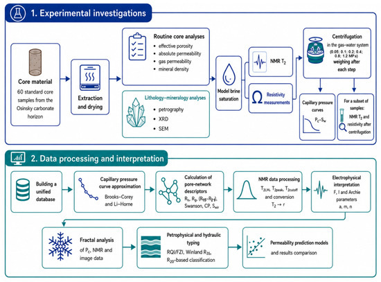
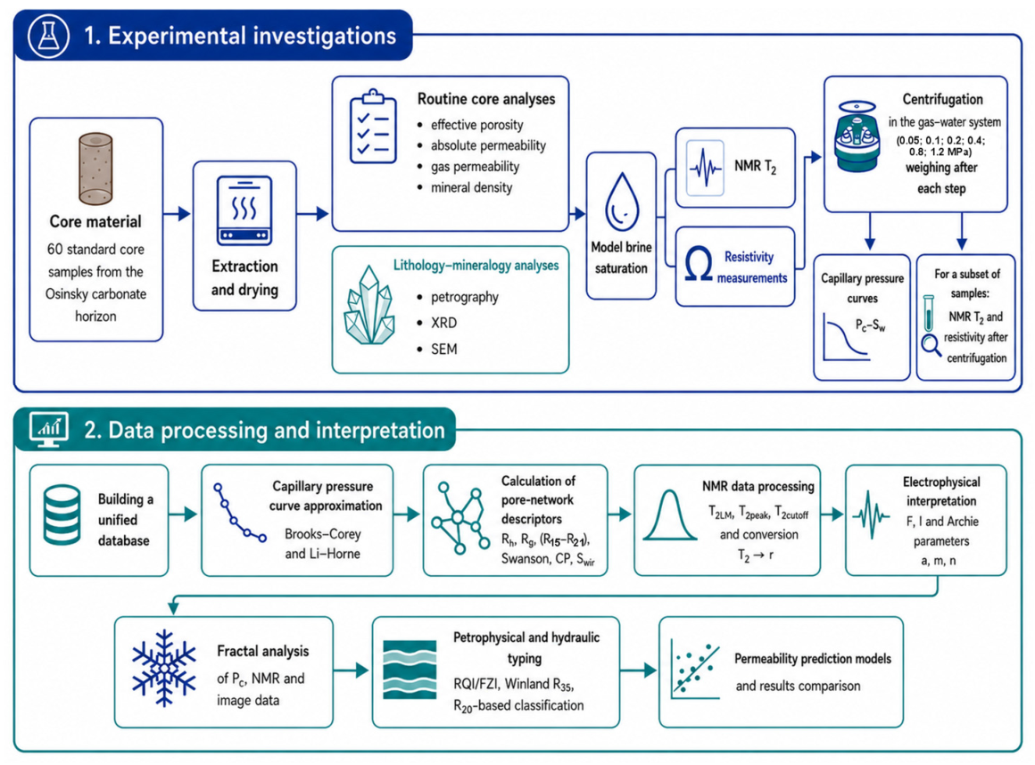
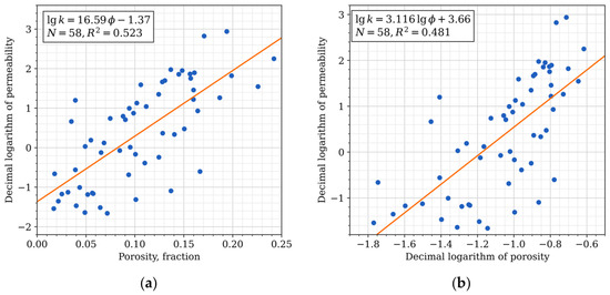
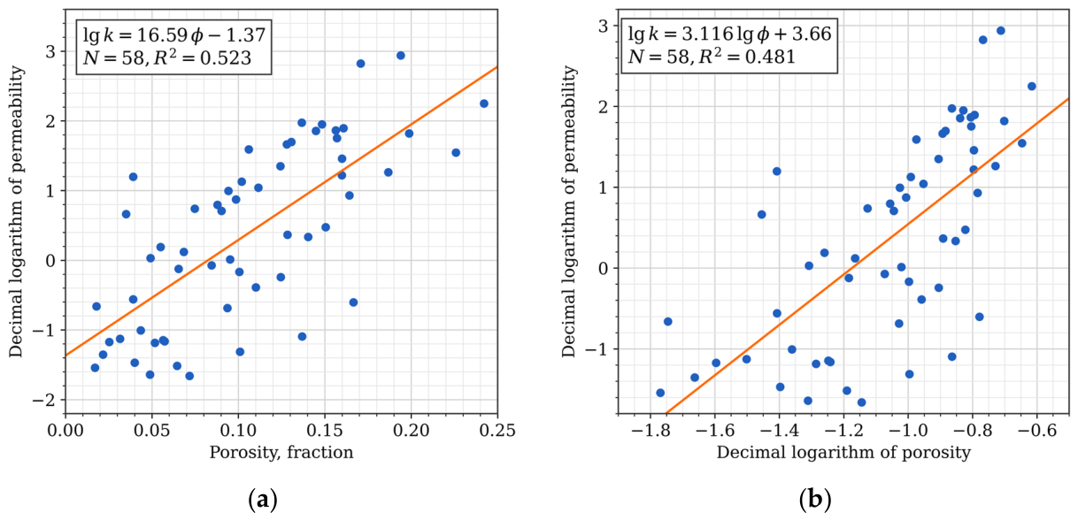
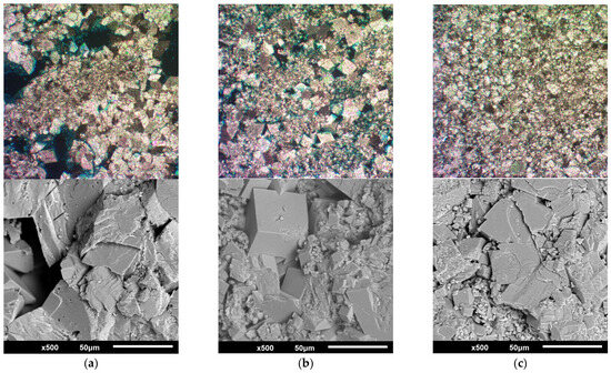
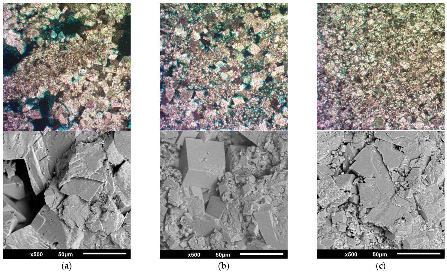
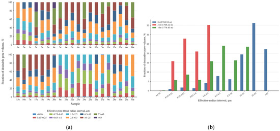
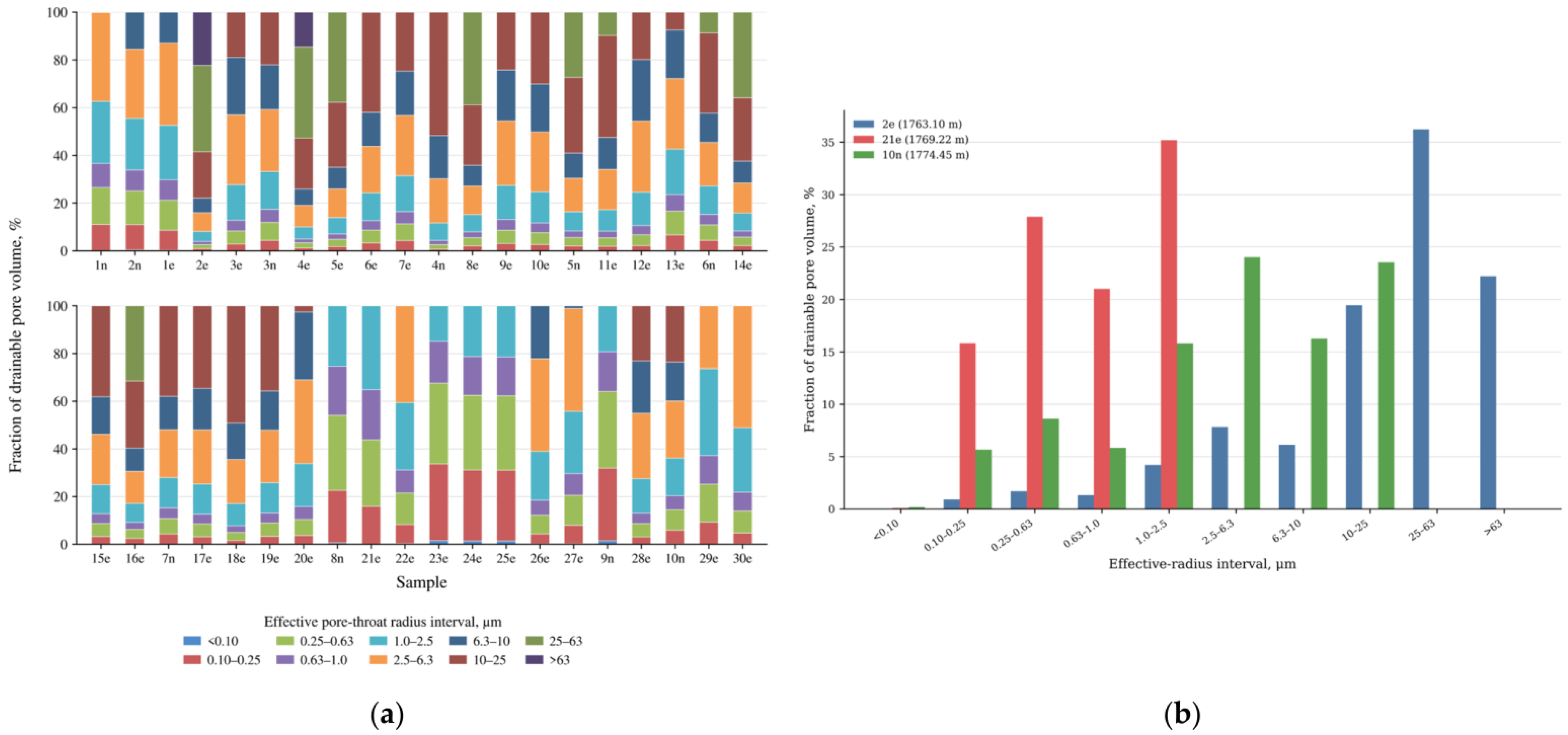
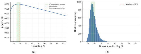
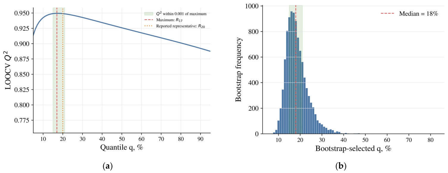
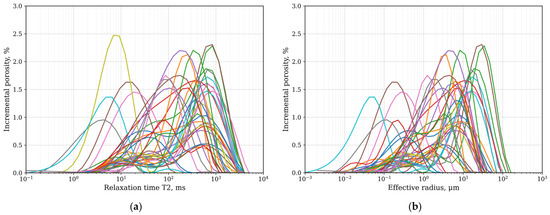
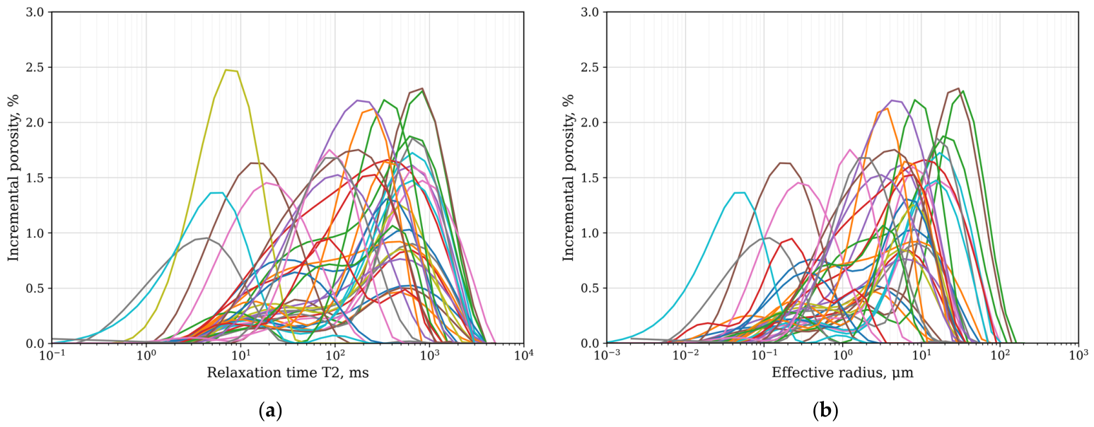
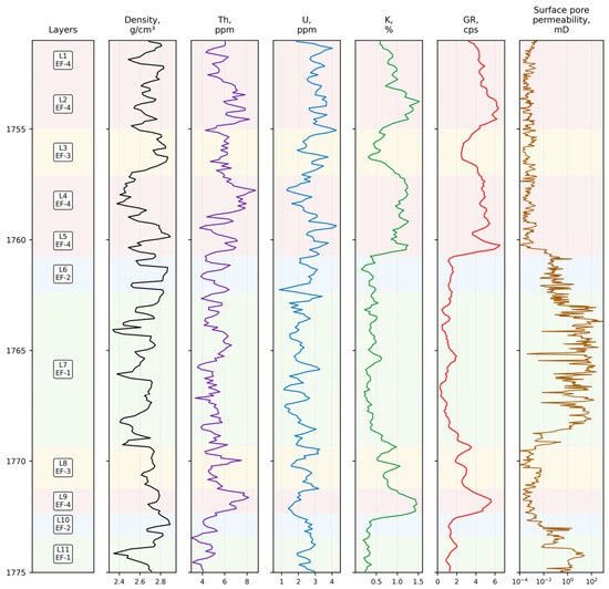
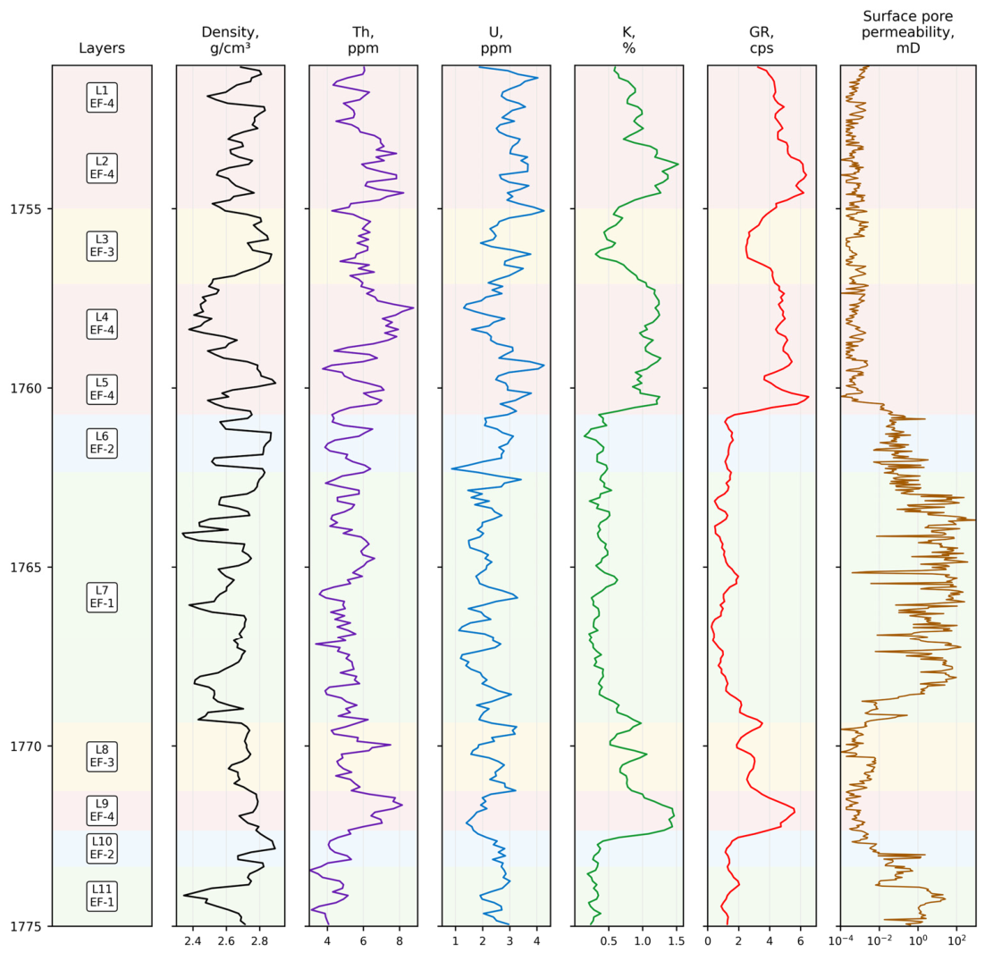
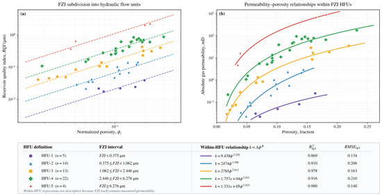
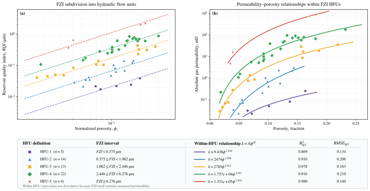
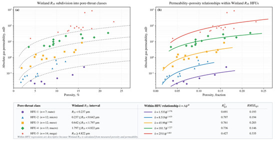
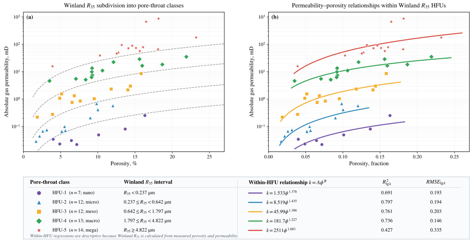
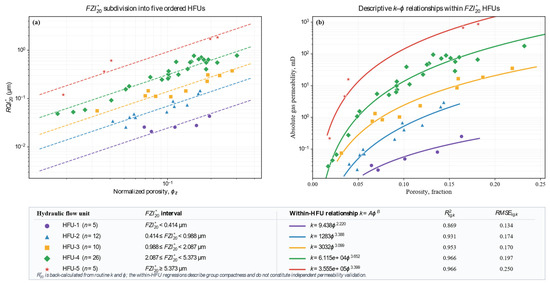
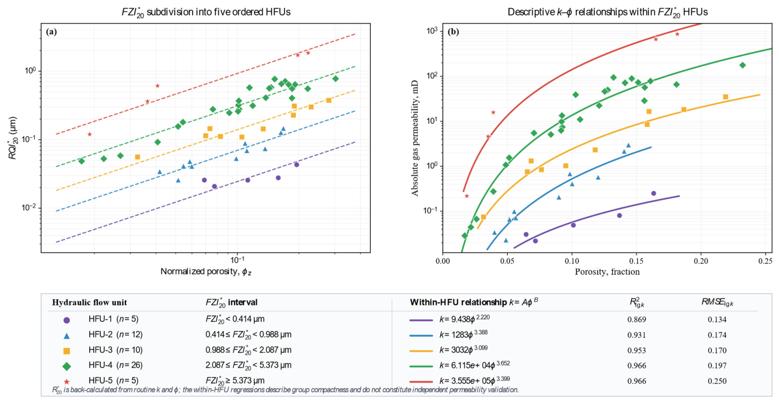
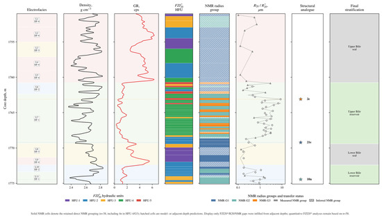
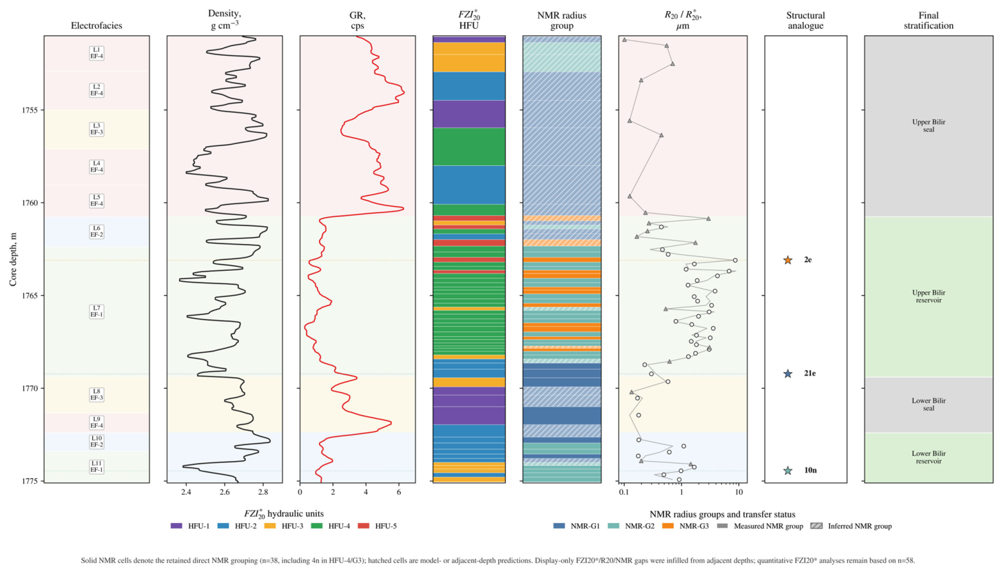
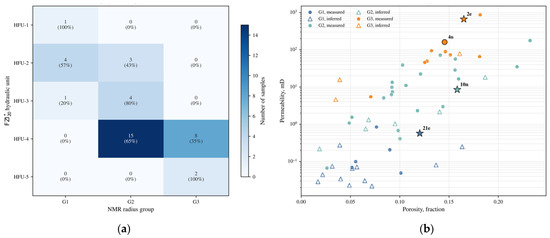
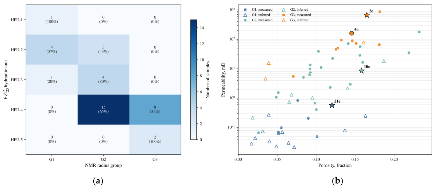

Disclaimer/Publisher’s Note: The statements, opinions and data contained in all publications are solely those of the individual author(s) and contributor(s) and not of MDPI and/or the editor(s). MDPI and/or the editor(s) disclaim responsibility for any injury to people or property resulting from any ideas, methods, instructions or products referred to in the content. |
© 2026 by the authors. Licensee MDPI, Basel, Switzerland. This article is an open access article distributed under the terms and conditions of the Creative Commons Attribution (CC BY) license.