Hybrid Fuzzy Convolutional Neural Networks for Photovoltaic Panel Anomaly Detection and Energy Optimization

Abstract

Convolutional Neural Networks (CNNs) are fundamental tools for image analysis and recognition in monitoring systems, particularly in photovoltaic (PV) installations, where visual inspection and thermal imaging play crucial roles in anomaly detection and energy optimization. This publication presents a Hybrid Fuzzy Convolutional Neural Network (HFCNN) that integrates a fuzzy dense layer utilizing Ordered Fuzzy Numbers (OFNs) into the CNN architecture. The architecture is additionally validated on the public ELPV benchmark of 2624 electroluminescence images of photovoltaic cells, where the HFCNN with Mean of Maxima defuzzification attains classification quality statistically indistinguishable from a CNN baseline while using a four times smaller dense layer and training two to three times faster. The methodology combines the feature extraction capabilities of traditional CNNs with the uncertainty handling properties of fuzzy logic. Experiments using the MNIST dataset demonstrate that HFCNN with Mean of Maxima (MOM) defuzzification achieves comparable accuracy to standard CNNs while using significantly fewer parameters (75% reduction in the dense layer). This efficiency gain is advantageous for deployment on edge computing devices. This work constitutes a methodological contribution—establishing, for the first time, the feasibility of integrating Ordered Fuzzy Numbers into CNN architectures without requiring expert membership function design. While the current study validates this approach on MNIST, actual photovoltaic applications require dedicated future research on real PV thermal imagery. Nevertheless, the proposed HFCNN framework could potentially support practical photovoltaic energy system applications in detecting panel degradation, performance anomalies, and autonomous decision-making in large-scale PV installations.

1. Introduction

Convolutional Neural Networks (CNNs) are used for image analysis and recognition [1]. These networks extract hierarchical features and classify them, making them particularly applicable to monitoring systems across various operational contexts. In mobile systems, such as vehicles, aircraft, and reconnaissance drones, CNNs enable real-time threat detection and classification, facilitating rapid alarm generation during mission operations.

Photovoltaic (PV) installations represent one of the most important renewable energy technologies, and their effective monitoring requires advanced analysis techniques. Observation systems in PV installations can utilize visual cameras, thermal imaging, or multispectral imaging modalities. For each imaging type, specialized CNNs can be developed for anomaly detection [2]. By integrating these networks with monitoring and control systems, operators can optimize PV performance in real time. Consequently, CNNs are essential for autonomous monitoring and decision-support in large-scale PV installations.

Among widely used CNN architectures are YOLO and ResNet. These networks process images through successive layers, progressively extracting and refining features. Early layers detect low-level features such as edges and textures, while deeper layers capture increasingly complex patterns and semantic information. Simultaneously, dimensionality reduction is performed to consolidate feature representations. The final layer serves as a classifier, assigning images to specific classes based on extracted features and performing either classification or regression tasks [1]. The term “Convolutional Neural Network” derives from the convolution operation, which is central to feature extraction. Images are represented as 2D matrices, where element values correspond to pixel intensities. The convolution operation applies a learned kernel (filter) across the image, computing element-wise products between kernel weights and image patches, followed by summation to produce feature maps [2]. Multiple kernels are applied in parallel, generating diverse feature representations.

One particularly promising approach involves integrating fuzzy neural networks with CNN architectures to leverage the strengths of both methodologies. Such hybrid systems are well-suited for PV energy optimization applications, enabling real-time anomaly detection and autonomous decision-making. Critically, reduced network size implies lower computational requirements, enabling deployment on resource-constrained processors and extending battery life in distributed PV systems.

Motivated by these requirements, the present work extends the original methodological proposal in two directions. First, the learning procedure of the fuzzy dense layer is formalized: Section 4.1 derives the forward pass, the gradient flow through the defuzzification operators, and the parameter-update rule used in the implementation. Second, the architecture is validated on real photovoltaic imagery. The publicly available ELPV benchmark of electroluminescence (EL) images of solar cells [3,4] is used to compare the HFCNN with a conventional CNN, an enlarged CNN variant, classical machine-learning baselines, and a lightweight transfer-learning model (MobileNetV3-Small [5]) under a common multi-seed statistical protocol and at two input resolutions. The MNIST experiments are retained as a controlled ablation study of the defuzzification operators.

2. State of the Art

In this section, a short review of publications on Convolutional Neural Networks is provided. In Ref. [6], an elementary understanding of CNN components and their functions is presented. This includes input layers, convolution layers, pooling layers, activation functions, batch normalization, dropout, fully connected layers, and output layers. The paper provides a comprehensive overview of the past and current research status of CNN applications in computer vision fields, such as image classification, object detection, and video prediction. In Ref. [7], Lightweight Deep Convolutional Neural Networks (LDCNNs) are discussed. These networks are particularly suited for mobile intelligence applications, especially in mobile vision.

In Ref. [8], a comprehensive review of CNN hyperparameters is provided. The authors categorize ten hyperparameter optimization algorithms into four classes. In Ref. [9], the authors present CNN as a machine-learning algorithm for automatic image classification. The system is applied to classify digit classes from the MNIST dataset, achieving a 98% accuracy rate. In Ref. [10], image classification was also performed using a type-2 fuzzy neural network that benefits from a Gaussian regression model. Another fuzzy solution connected with convolutional networks for image classification was proposed in Ref. [11]. In medical image recognition, fuzzy logic proved helpful for classifying objects where ordinary convolutional networks encountered difficulties due to indistinct boundaries [12].

In Ref. [13], the authors reviewed CNNs and presented the YOLO (You Only Look Once) network solution. In short, the YOLO network divides the image area into smaller segments and then searches for so-called bounding boxes within them, performing image classification afterward. The main advantage of YOLO is its high processing speed. In Ref. [14], it was shown that the processing speed of the YOLO network can be up to 300 times faster than that of Fast-RCNN. However, the training time of the network depends on the dataset and, of course, the hardware used [15].

YOLO-based solutions are suitable for use in real-time systems [16]. It is possible to recognize a wide variety of objects—from license plates [17], through traffic analysis [18], to applications in agriculture [19]. The most recent version of YOLO is version 11 [20]. Over the years, the versions have evolved, providing increasingly better quality and processing speed [21]. It is also worth noting that the solution has been studied for thermal images [22], which is particularly relevant for photovoltaic panel monitoring.

Another widely used and well-researched solution is the ResNet network. Many medical applications can be found, such as skin anomaly detection [23]. Other applications found in the literature include detection of anomalies in photovoltaic panels [24], drones and satellite imagery [25,26], detection of railway track damage [26], fruit freshness analysis [27], and waste classification [28]. The applications of ResNet networks are therefore also very broad and depend only on specific needs.

One particularly interesting solution is the use of fuzzy networks, especially fuzzy neural networks for image analysis. There are also hybrid solutions built upon existing architectures [29]. Such a network leverages the advantages of fuzzy logic mechanisms to achieve better classification results.

VGG networks have been effectively used for detecting defects in PV because of their simplicity. Recent studies demonstrate exceptional performance, with comprehensive studies using VGG16 and VGG19 architectures for solar panel fault detection [30]. A hybrid approach combining VGG16 with the Bitterling Fish Optimization (BFO) algorithm achieved outstanding results with 98.75% accuracy, 98.72% sensitivity, and 98.78% specificity [31]. The combination of the VGG19 network with thermal imaging is a good approach for detecting faults in photovoltaic panels, and attention mechanisms help accurately identify where the problem is located [32]. These approaches showcase the continued relevance of classical CNN architectures when properly optimized.

Residual networks have emerged as powerful architectures for PV defect detection, particularly when enhanced with specialized modules. The improved VarifocalNet framework utilizing ResNet-101 as a backbone addresses the challenge of detecting small defects in electroluminescence images [33]. This approach outperforms standard detection methods, including RetinaNet, Faster R-CNN, and Cascade R-CNN, on the PVEL-AD dataset. Most recently, ResNet-based image processing approaches for precise crack detection in PV panels have been developed, demonstrating automated defect detection capabilities with high accuracy [34]. These advancements highlight the effectiveness of residual connections in capturing multi-scale features critical for defect localization.

Lightweight architectures are increasingly important for edge deployment in distributed PV systems. EfficientNet-B0 has demonstrated remarkable performance in detecting defective PV modules, achieving 97.81% accuracy on the PVEL dataset when combined with contrast-limited adaptive histogram equalization (CLAHE) [35]. The model’s ability to scale across depth, width, and resolution while maintaining computational efficiency makes it ideal for real-time inspections. Enhanced EfficientNet-V2 architectures have also shown superior defect identification capabilities in high-noise environments and dust storms [36]. SqueezeNet, another lightweight alternative, has achieved comparable results with even smaller model sizes. These lightweight models are particularly valuable for deployment on edge computing devices at distributed PV installation sites.

For real-time defect localization, object detection networks have proven highly effective. YOLOv7 enhanced with Partial Convolution and Switchable Atrous Convolution techniques provides fast and accurate anomaly detection in PV cells, effectively managing image irregularities and varying defect scales [37]. Recent implementations of YOLOv8 with specialized global and depthwise modules (YOLOv8-GD) have improved detection in electroluminescence images, while YOLOv11 continues to advance architectural enhancements [38]. Faster R-CNN and Cascade R-CNN variants provide more refined detection at the cost of increased computational complexity. The choice between these architectures depends on the specific application requirements regarding speed versus accuracy trade-offs.

Recent advances have introduced novel hybrid architectures combining multiple techniques. SolarAttnNet presents a novel CNN architecture with integrated channel and spatial attention mechanisms for solar panel anomaly detection [39], leveraging attention to emphasize the most relevant features in thermal and visual imagery. HybridSolarNet combines EfficientNet with Convolutional Block Attention Modules (CBAMs) for lightweight, explainable, real-time solar panel fault detection. Furthermore, hybrid CNN-Fuzzy approaches have demonstrated effectiveness in automatic identification of complex patterns and can be adapted for PV defect classification [29]. These hybrid approaches represent the cutting edge of CNN architecture design for specialized applications.

Electroluminescence imaging is the most widely used technique for detecting internal defects in PV cells. The PVEL-AD dataset contains 36,543 near-infrared EL images featuring various defects, including cracks, finger scratches, black cores, and dislocations [40]. The ELPV dataset provides 2624 grayscale images extracted from EL images of 44 different solar modules, annotated with defect probabilities [3]. These large-scale datasets have enabled comprehensive benchmarking of CNN architectures. In EL images, defects appear as dark gray lines and areas, making them particularly suitable for deep learning-based detection. The availability of these public datasets has significantly accelerated research progress in this field.

Thermal infrared imaging via unmanned aerial vehicles (UAVs) has become an efficient method for inspecting large-scale PV plants, detecting hotspots, electrical disconnections, and short-circuited cells. A multimodal approach combining infrared, electroluminescence, and RGB imaging has demonstrated the ability to identify 21 distinct types of defects with high accuracy [41]. The Infrared Solar Module dataset enables evaluation of CNN robustness against orientation changes and luminance variations caused by varying UAV flight paths and weather conditions. Visible spectrum (RGB) imaging identifies surface-level defects, including glass breakage, soiling, and vegetation shading. Multimodal fusion approaches, combining thermal, electroluminescence, and RGB images, provide comprehensive defect detection capabilities that significantly outperform single-modality approaches.

The PVEL-AD dataset is the largest publicly available dataset for PV cell anomaly detection, containing 36,543 near-infrared electroluminescence images with heterogeneous backgrounds [40]. It includes 40,358 ground-truth bounding boxes annotated for 12 defect types: crack (line and star), finger interruption, black core, thick line, scratch, fragment, corner, printing error, horizontal dislocation, vertical dislocation, and short-circuit defects. This long-tail object detection task provides a challenging and significant benchmark for smart manufacturing applications. The ELPV dataset contains 2624 grayscale electroluminescence images extracted from high-resolution EL images of 44 different solar modules [3]. Each image is 300 × 300 pixels representing functional or defective solar cells, annotated with defect probability (0–1) and solar module type (mono- or polycrystalline). This dataset has been instrumental in validating transfer learning approaches, with CNN achieving 88.42% average accuracy on these images. The Infrared Solar Module dataset comprises thermal infrared images captured via drone-based inspection of PV installations, emphasizing robustness evaluation under realistic field conditions, including varying illumination, weather changes, and UAV flight path variations.

Transfer learning has become crucial for improving CNN performance on PV datasets, particularly when labeled data is limited. Pretrained models on ImageNet weights provide a strong initialization, reducing training time and improving accuracy. Fine-tuning strategies involving layer freezing and selective unfreezing of deeper layers have proven effective for PV-specific applications. Recent approaches employ advanced data augmentation techniques, synthetic data generation, and domain adaptation methods to bridge the gap between synthetic training images and real-world field conditions. Ensemble methods combining multiple pretrained models (GoogleNet, SqueezeNet, ResNet-50, VGGNet-16, AlexNet) with feature selection algorithms like Bitterling Fish Optimization further enhance classification performance [31]. These strategies have been shown to reduce overfitting and improve generalization to unseen defect types.

Several significant challenges remain in PV anomaly detection that warrant future research. Data heterogeneity represents a fundamental obstacle, as PV modules exhibit high variability in manufacturing, environmental conditions, and degradation patterns, requiring models robust to domain shift [41]. Class imbalance is another critical issue, where defective images are relatively rare compared to normal images, necessitating advanced sampling and weighting strategies. Optimal integration of thermal, electroluminescence, and RGB data remains an open problem requiring more sophisticated fusion architectures. Models must maintain performance under field conditions, including dust, weather variations, and partial shading [36]. Interpreting CNN decisions for regulatory compliance and maintenance planning remains challenging from an explainability perspective. Emerging Vision Transformer architectures show promise for capturing long-range dependencies in defect patterns, requiring further investigation and comparison with traditional CNNs.

Convolutional Neural Networks have become indispensable tools for automating PV anomaly detection, with recent advances achieving accuracies exceeding 98% on benchmark datasets. VGG, ResNet, EfficientNet, and YOLO architectures each offer distinct advantages in accuracy, speed, and efficiency trade-offs. The availability of large-scale public datasets (PVEL-AD, ELPV) has accelerated research progress and enabled comprehensive benchmarking. Transfer learning and hybrid approaches combining multiple architectures demonstrate superior performance compared to single-architecture approaches. However, significant challenges remain regarding data heterogeneity, real-world deployment, and multimodal integration. Future research should focus on developing robust, explainable models capable of handling domain shift and field conditions while maintaining computational efficiency for edge deployment in distributed PV systems. The convergence of advanced architectures, larger datasets, and transfer learning strategies suggests that fully autonomous PV system monitoring is increasingly feasible.

3. Hybrid Fuzzy Convolutional Neural Network with Ordered Fuzzy Numbers

FALCON and ANFIS represent prominent fuzzy neural architectures widely employed in machine-learning applications [42]. The FALCON architecture was introduced by Lin and Lee [43]. Both systems utilize two distinct parameter classes during training: connection weights and membership function characteristics. The training procedure employs a sequential two-phase approach: first, connection weights are adjusted while membership functions remain fixed; subsequently, membership function parameters are optimized using gradient descent while weights maintain their previously determined values. Unfortunately, this decoupled training strategy may produce suboptimal results for certain problem classes, as the approach assumes relative independence between the two parameter sets. In practice, however, these parameter classes exhibit strong interdependence [43,44,45], limiting the effectiveness of the sequential optimization approach.

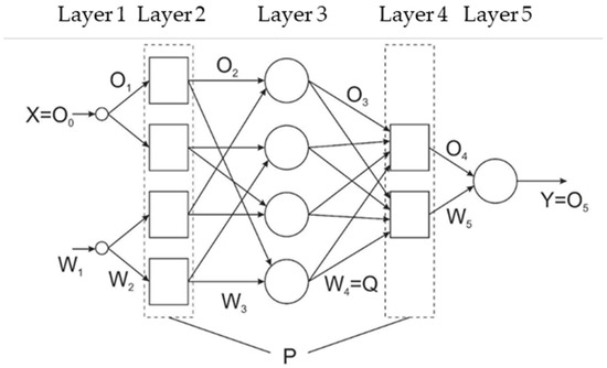
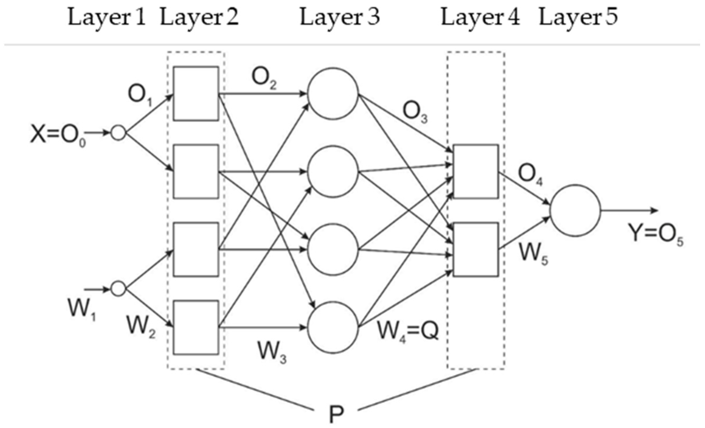
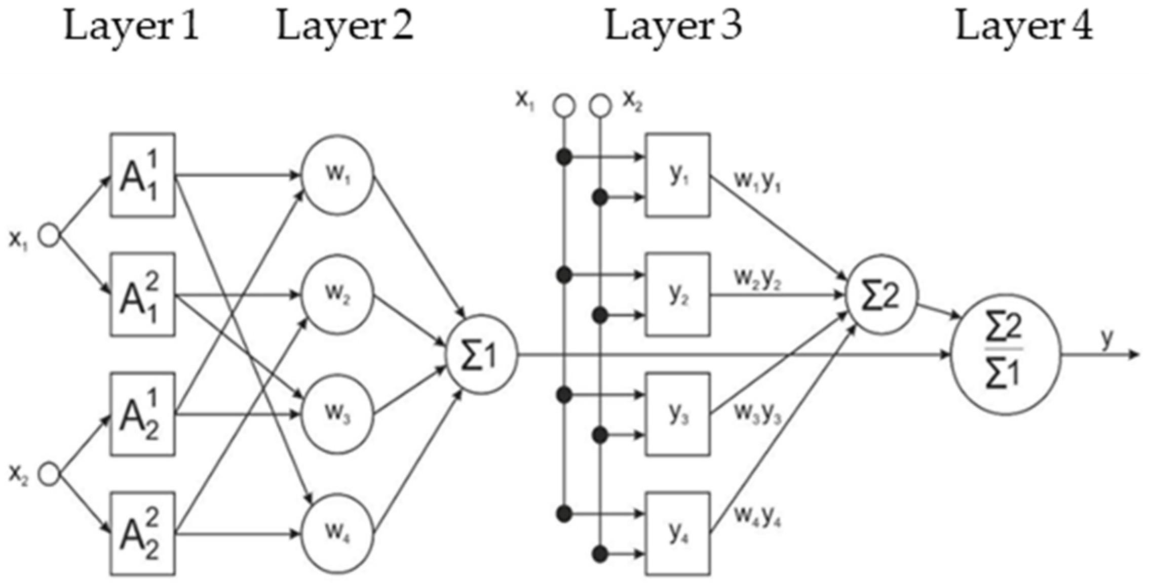
The FALCON/ANFIS network architecture comprises five functional layers (Figure 1). The input layer performs data fuzzification, converting crisp inputs into fuzzy representations. The second layer evaluates antecedent conditions (IF components) of fuzzy inference rules. The third layer encodes the inference rule base. The fourth layer implements consequent actions (THEN components) based on rule activations. Finally, the fifth layer performs defuzzification, converting fuzzy outputs to crisp values.

Figure 1. FALCON network architecture.

The ANFIS architecture encodes fuzzy inference rules through a parameter matrix Q, containing the consequent weights. Membership functions are defined by Gaussian distributions, characterized by two parameters: the mean (center) and standard deviation (width). These membership function parameters are organized in matrix P, where each row corresponds to a membership function, and columns represent the mean and standard deviation for the corresponding input or output variable. The task of the network is to calculate the mapping F of the input vector X into the output vector Y, using P and Q:

Y = F (X, P, Q).

(1)

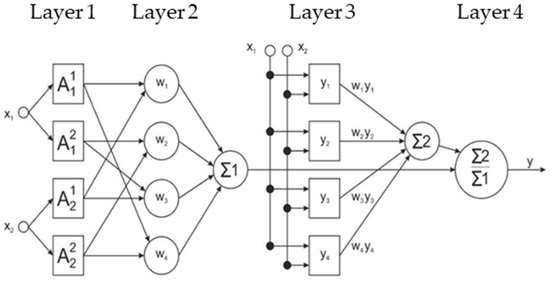
The Adaptive Neuro-Fuzzy Inference System (ANFIS) [46] is a hybrid architecture combining neural network learning capabilities with fuzzy inference mechanisms. ANFIS training employs a sophisticated hybrid algorithm that optimizes two distinct parameter sets through different mechanisms: consequent parameters are optimized in the forward pass using least-squares estimation, while antecedent parameters (membership function characteristics) are refined in the backward pass via gradient descent. This dual optimization strategy enables efficient convergence by leveraging the complementary strengths of statistical and gradient-based methods. Figure 2 depicts an ANFIS architecture configured with a uniformly partitioned 2D input space, illustrating how the fuzzy rule-base and membership functions are structured for this representative example.

Figure 2. The scheme of fuzzy ANFIS with rectangular division of the two-dimensional input space [47].

Numerous ANFIS implementations are available in open-source software repositories, including well-documented solutions for benchmark tasks such as Iris dataset classification. Implementations exist for both R 4.0.5 and Python 3.13.7 programming languages [47].

The primary distinction between ANFIS and standard deep learning frameworks lies in the explicit definition of membership functions. Unlike deep networks, where feature representations are learned automatically, ANFIS requires manual specification of membership function parameters. For example, the code invocation make_gauss_mfs (1, [−5, 0.08, 1.67]) initializes a Gaussian membership function with specified mean and standard deviation values. The choice of these parameters—their centers, widths, and number—critically influences network performance and requires domain expertise to optimize effectively.

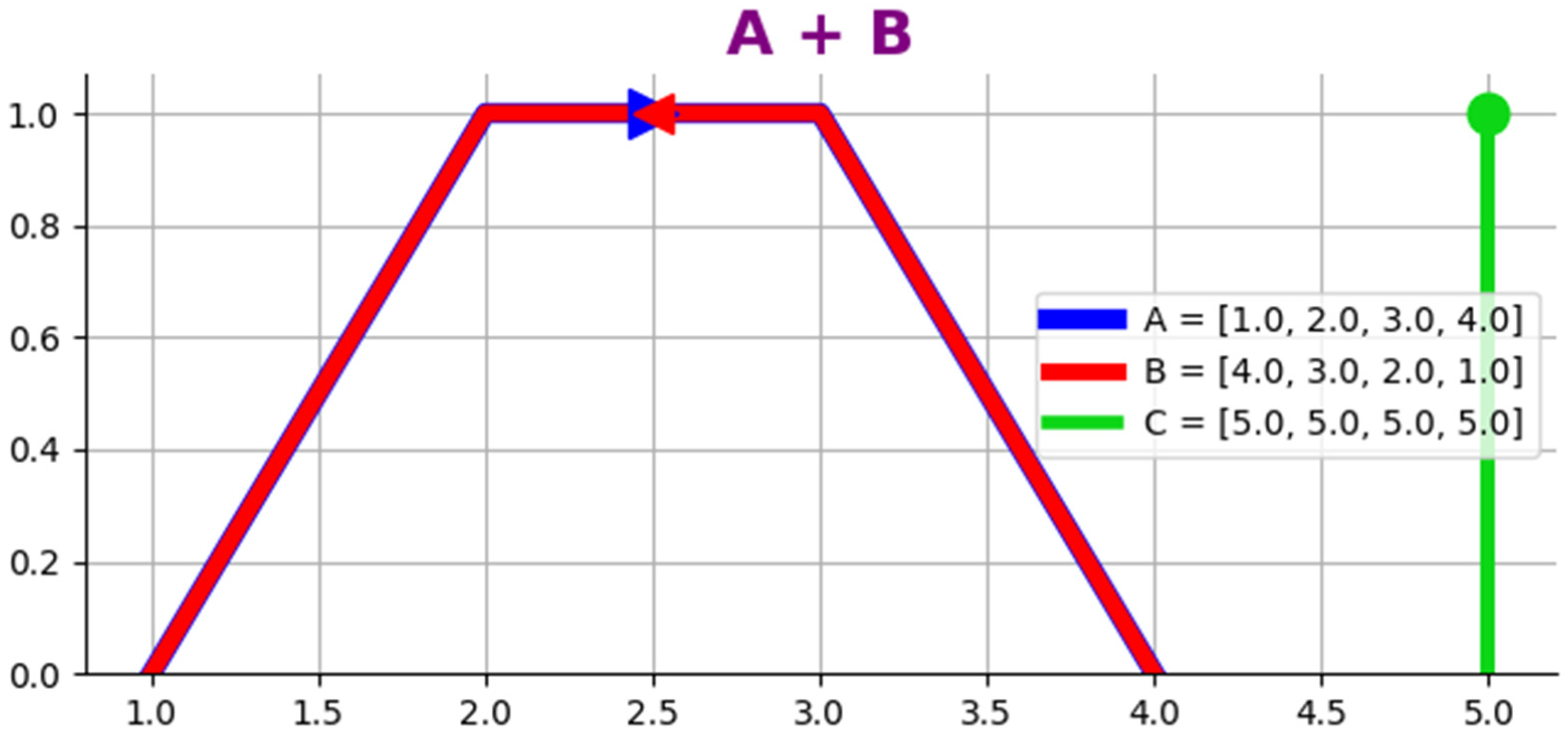
The proposed Hybrid Fuzzy Convolutional Neural Network is different. It uses Ordered Fuzzy Number (OFN, Figure 3), which is an ordered pair $A=\left(f_A{,g}_A\right)$ continuous functions $F:f_A{,g}_A:\left[0,1\right]\to R$ referred to, respectively, as parts:

• ${up}_A$_A—beginning, rising slope;
• ${down}_A$—end, falling slope.

Figure 3. Example of the Ordered Fuzzy Number: A—positive, B—negative, C—singleton.

Figure 3. Example of the Ordered Fuzzy Number: A—positive, B—negative, C—singleton.

Basic arithmetic operations on Ordered Fuzzy Numbers:

• Sum: Ordered Fuzzy Number $C=\left(f_C{,g}_C\right)$ is a sum of numbers $A=\left(f_A{,g}_A\right)$ and $B=\left(f_B{,g}_B\right)$, when:

$${\forall }_{y\in \left[\mathrm{0,1}\right]}\left[f_A\left(y\right)+f_B\left(y\right)=f_C\left(y\right) \wedge g_A\left(y\right)+g_B\left(y\right)=g_C\left(y\right)\right],$$

(2)

• Difference: Ordered Fuzzy Number $C=\left(f_C{,g}_C\right)$ is a difference of numbers $A=\left(f_A{,g}_A\right)$ and $B=\left(f_B{,g}_B\right)$, when:

$${\forall }_{y\in \left[\mathrm{0,1}\right]}\left[f_A\left(y\right)-f_B\left(y\right)=f_C\left(y\right) \wedge g_A\left(y\right)-g_B\left(y\right)=g_C\left(y\right)\right],$$

(3)

• Multiplication by a scalar: Ordered Fuzzy Number $C=\left(f_C{,g}_C\right)$ is the result of multiplying a number $A=\left(f_A{,g}_A\right)$ by scalar $r\in R$, when:

$${\forall }_{y\in \left[\mathrm{0,1}\right]}\left[{r·f}_A\left(y\right)=f_C\left(y\right) \wedge r·g_A\left(y\right)=g_C\left(y\right)\right],$$

(4)

• Product: Ordered Fuzzy Number $C=\left(f_C{,g}_C\right)$ is a product of numbers $A=\left(f_A{,g}_A\right)$ and $B=\left(f_B{,g}_B\right)$, when:

$${\forall }_{y\in \left[\mathrm{0,1}\right]}\left[f_A\left(y\right)·f_B\left(y\right)=f_C\left(y\right) \wedge g_A\left(y\right)·g_B\left(y\right)=g_C\left(y\right)\right],$$

(5)

• Quotient: Ordered Fuzzy Number $C=\left(f_C{,g}_C\right)$ is a quotient of numbers $A=\left(f_A{,g}_A\right)$ by $B=\left(f_B{,g}_B\right)$, when:

$${\forall }_{y\in \left[\mathrm{0,1}\right]}\left[f_A\left(y\right)/f_B\left(y\right)=f_C\left(y\right) \wedge g_A\left(y\right)/g_B\left(y\right)=g_C\left(y\right)\right],$$

(6)

While fuzzy neural networks have been extensively studied in prior work [42], no previous research has integrated Ordered Fuzzy Numbers (OFNs) arithmetic into neural network architectures. We selected OFNs for this application because:

• OFN representations mitigate known limitations of traditional L-R fuzzy numbers, enabling more efficient and stable computations;
• To our knowledge, no prior work has implemented neural networks utilizing OFN arithmetic, making this approach novel and unexplored.

We propose a modified McCulloch–Pitts neuron model that processes inputs, weights, and outputs as Ordered Fuzzy Numbers rather than crisp scalars [15]. This representation naturally captures imprecision and uncertainty in numerical computations. OFN arithmetic operations are executed through a two-step process, enabling seamless integration with standard backpropagation training procedures:

Step 1: The calculation involves multiplying the input values by their corresponding weights and then adding up the products to obtain a final value:

$$S=W_0+ {\sum }_{i=0}^n{X}_i{W}_i,$$

(7)

Step 2: Then the output using OFN arithmetic is calculated as follows:

$$Y=f\left(S\right).$$

(8)

The elements within S, W, X, and Y are represented as values in OFN notation. This methodology necessitates subsequent layers to be implemented:

• First layer—A fuzzification process is employed to convert input data into the network into OFN notation;
• Last layer—Defuzzification is utilized for processing the output data from the network;
• Deep layer—Network learning/training algorithms are adapted to operate effectively with OFN network arithmetic in network layers.

We integrated a Dense Fuzzy Layer operating in Ordered Fuzzy Number notation to investigate whether comparable accuracy could be achieved relative to standard CNNs while significantly reducing network size.

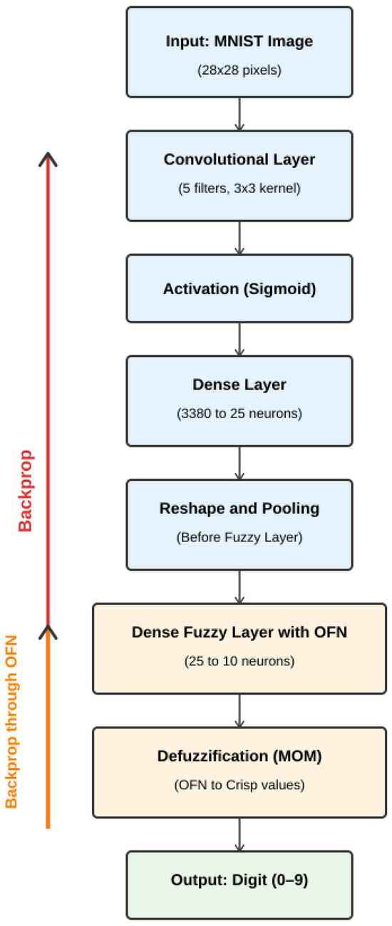
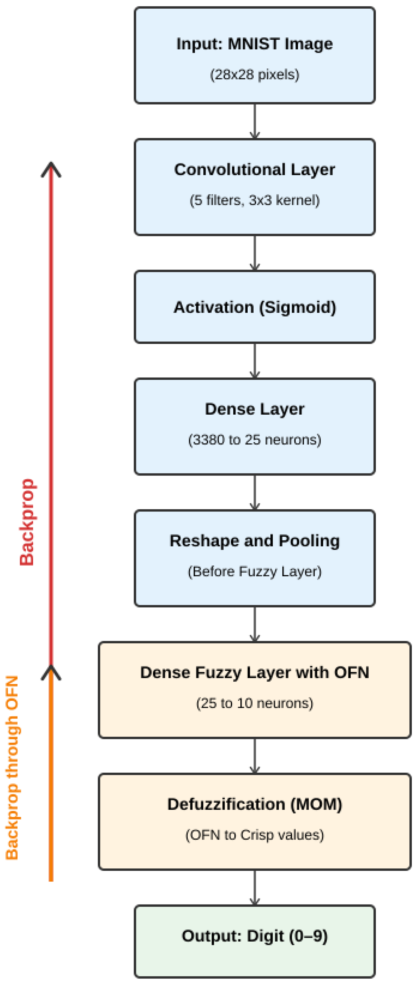
Figure 4 illustrates the complete network architecture. Input images are processed sequentially through the following stages: (1) convolutional layers extract spatial features; (2) a reshaping layer transforms the 3D feature maps into a 1D vector; (3) a standard dense layer further abstracts these features; and (4) a Dense Fuzzy Layer performs classification using OFN arithmetic. The Dense Fuzzy Layer represents the novel component, performing all computations in Ordered Fuzzy Number space. Neuron inputs, weights, and activations are represented as OFN pairs rather than scalars, enabling natural uncertainty representation throughout the layer. A selected defuzzification method (specifically Mean of Maxima) converts the final OFN outputs to crisp class predictions.

Figure 4. Hybrid Fuzzy Convolutional Neural Network: Image as an input into the convolutional layer, the result of this layer is reshaped by a reshape layer, then a dense layer prepares data into a fuzzy dense layer, which provides the network output.

The baseline CNN architecture (Table 1) was implemented in standard form to enable reproducible baseline comparisons. This network comprises three processing stages: convolutional feature extraction, intermediate data processing, and two fully connected layers. We also evaluate CNN4, an enlarged variant where the dense layer is four times larger, serving as an over-parameterized control.

Table 1. The CNN, HFCNN, and CNN4 architectures.

CNN Architecture	HFCNN Architecture	CNN4 Architecture
network = [	network = [	network = [
Convolutional((1, 28, 28), 3, 5),	Convolutional((1, 28, 28), 3, 5),	Convolutional((1, 28, 28), 3, 5),
Sigmoid(),	Sigmoid(),	Sigmoid(),
Reshape((5, 26, 26),	Reshape((5, 26, 26),	Reshape((5, 26, 26),
(5 × 26 × 26, 1)),	(5 × 26 × 26, 1)),	(5 × 26 × 26, 1)),
Dense(5 × 26 × 26, 100),	Dense(5 × 26 × 26, 25),	Dense(5 × 26 × 26, 400),
Sigmoid(),	Sigmoid(),	Sigmoid(),
Dense(100, 10),	DenseOFN(25, 10),	DenseOFN(400, 10),
Sigmoid() ]	Sigmoid() ]	Sigmoid() ]

The proposed Hybrid Fuzzy Convolutional Neural Network (HFCNN) adopts the same upstream architecture as the baseline CNN but replaces the final dense layer with a Dense Fuzzy Layer implementing Ordered Fuzzy Number arithmetic. This fuzzy layer contains 25% of the parameters of the corresponding CNN layer, enabling investigation of whether parameter-efficient architectures can maintain competitive accuracy.

Our primary objective was to determine whether comparable accuracy could be achieved relative to standard CNNs while substantially reducing network size. The Dense Fuzzy Layer represents the novel architectural component. Unlike standard dense layers performing scalar arithmetic, this layer maintains fuzzy uncertainty throughout computation: neuron inputs, weights, and activations are represented as Ordered Fuzzy Number pairs. A defuzzification method converts final OFN outputs to crisp class predictions. This design enables natural uncertainty representation without requiring expert membership function design, a key distinction from traditional fuzzy systems such as ANFIS.

4. Methodology

As part of the research, the MNIST dataset, containing handwritten digits, was used. A standard convolutional network and a convolutional network with a deep fuzzy layer, referred to as HFCNN, were prepared. For testing purposes, a random selection of 1000 training images and 200 test images was made. The training parameters of the network were as follows: the binary cross-entropy function was used as the loss function, the training process was conducted over 50, 100, 150, 200, and 250 epochs, and the learning rate was set to 0.05.

In addition, the Hybrid Fuzzy Convolutional Neural Network was evaluated using different defuzzification (sharpening) methods: FOM (First of Maxima), LOM (Last of Maxima), and MOM (Mean of Maxima). Sharpening (defuzzification) operators were derived accordingly [48]:

• FOM—First of Maxima, an operator that returns the smallest element of the core of a fuzzy set A

FOM(A) = min core(A),

(9)

• LOM—Last of Maxima, an operator whose result is the largest element of the core of a fuzzy set A

LOM(A) = max core(A),

(10)

• MOM—Mean of Maxima, an operator whose result is the arithmetic mean of the smallest and largest elements of the core of a fuzzy set

MOM(A) = (min core(A) + max core(A))/2

(11)

As can be seen from the formulas, the FOM, LOM, and MOM methods do not take into account the orientation that directed fuzzy numbers possess. Considering the definition of Ordered Fuzzy Numbers—in particular, the fact that the value of function f for 0 is f(0) and for 1 is f(1), and analogously, for function g these are g(0) and g(1)—sharpening (defuzzification) operators were derived accordingly [46]:

ΦFOM(f,g) = f(1),

(12)

ΦLOM(f,g) = g(1),

(13)

ΦMOM(f,g) = (f(1) + g(1))/2.

(14)

As part of the evaluation, the parameters accuracy, precision, recall, and F1-score were assessed.

To assess the statistical reliability of the results, each experiment was repeated 50 times with independent random weight initializations, and the tables report the mean values over these repetitions. In addition, for representative runs, the uncertainty resulting from the finite test set (n = 3000) was quantified: 95% confidence intervals for accuracy, macro-precision, macro-recall, and macro-F1 were estimated by non-parametric bootstrap resampling of the confusion matrix (5000 replicates), and the Wilson score interval was computed for accuracy. Differences in accuracy between network variants trained for the same number of epochs were tested with a two-proportion z-test at the significance level α = 0.05. Since all variants were evaluated on the same test set, this unpaired test is conservative. Repeated runs of the same configuration (HFCNN-MOM, 50 epochs) differed by up to 2.8 percentage points of accuracy, indicating that between-run variability due to random initialization is of a similar magnitude to the test-set uncertainty; the reported conclusions hold under both sources of variation.

In addition to the classification quality, the computational footprint of the networks was measured. Memory usage was recorded as the resident set size (RSS) of the Python process, obtained with the psutil library, and CPU utilization was read with psutil at the same points of program execution for each network: before and after data loading, before and after training, and after prediction. All measurements were taken on the same machine under identical conditions.

4.1. Backpropagation Through the OFN Dense Layer

Each weight of the fuzzy dense layer is an Ordered Fuzzy Number represented by four real components, w = (w⁽¹⁾, w⁽²⁾, w⁽³⁾, w⁽⁴⁾), corresponding to the discretized boundary values f(0), f(1), g(1), g(0) of the pair of functions (f, g). Biases are OFNs of the same form, whereas the layer input x is crisp, because it is produced by the preceding activation. Since the OFN sum and the product of an OFN with a scalar act independently on each component, the pre-activation of neuron o is an OFN whose components are given by four parallel affine maps:

$$z_o^{\left(c\right)}={\displaystyle \sum _{i=1}^n}{w}_{oi}^{\left(c\right)}{x}_i+b_o^{\left(c\right)}, c=1,\dots ,4,$$

(15)

where n is the input size. Before the activation function is applied, the fuzzy pre-activation is defuzzified by the selected operator Φ from Equations (12)–(14). Because all of these operators are linear in the four components, the defuzzified pre-activation can equivalently be written in terms of effective crisp weights: ẑ_o = Σ_i Φ(w_oi) x_i + Φ(b_o); the layer therefore acts on crisp data through Φ(w) while retaining the full four-component representation internally. Let δ_o denote the crisp error signal reaching the defuzzification boundary of neuron o, i.e., δ_o = (∂L/∂a_o)·σ′(ẑ_o). The exact gradients follow from the chain rule:

$${\displaystyle \frac{\partial L}{\partial w_{oi}^{\left(c\right)}}} = {\delta }_o{d}^{\left(c\right)}{x}_i, {\displaystyle \frac{\partial L}{\partial b_o^{\left(c\right)}}} = {\delta }_o{d}^{\left(c\right)}, {\displaystyle \frac{\partial L}{\partial x_i}} = \sum _o{\delta }_o\Phi \left(w_{oi}\right),$$

(16)

where d = (∂Φ/∂z⁽¹⁾, …, ∂Φ/∂z⁽⁴⁾) is the constant derivative vector of the defuzzification operator:

$$d_{\mathrm{M}\mathrm{O}\mathrm{M}} = (1, -{\displaystyle \frac{1}{2}}, {\displaystyle \frac{1}{2}}, 0), d_{\mathrm{F}\mathrm{O}\mathrm{M}} = (0, 1, 0, 0), d_{\mathrm{L}\mathrm{O}\mathrm{M}} = (0, 0, 1, 0).$$

(17)

The reference implementation applies a uniform component update, in which all four components of a weight receive the same increment:

$$w_{oi}^{\left(c\right)} \leftarrow w_{oi}^{\left(c\right)} - \eta {\delta }_o{x}_i, c = 1, \dots , 4.$$

(18)

Because every operator in Equations (12)–(14) satisfies Σ_c d^(c) = 1, the uniform rule (18) performs exact gradient descent on the effective crisp weights, Φ(w_oi) ← Φ(w_oi) − ηδ_ox_i, while preserving the initial fuzzy spread of each weight: the differences w⁽²⁾ − w⁽¹⁾ and w⁽⁴⁾ − w⁽³⁾ remain constant during training. Weights are initialized as w⁽¹⁾ ~ U(0, 1), w⁽²⁾ = w⁽¹⁾ + U(0, 1), w⁽³⁾ = w⁽²⁾, and w⁽⁴⁾ = w⁽³⁾ + U(0, 1). An important consequence is that, under the uniform update rule and this initialization, the Φ_FOM and Φ_LOM operators become mathematically equivalent—the corresponding components are identical at initialization and receive identical updates—so FOM and LOM networks trained from the same random seed produce bit-identical predictions. Moreover, the effective FOM/LOM weights differ from the MOM weights only by a frozen, non-negative random offset w⁽²⁾ − w⁽¹⁾, which explains the systematic advantage of MOM observed in Section 5. The fully orientation-aware variant, which updates each component with its own gradient from Equation (16), is also implemented in the released library and is left for a systematic comparison in future work.

4.2. Validation Protocol on the ELPV Photovoltaic Benchmark

To assess the applicability of the proposed architecture to photovoltaic monitoring, the networks were additionally validated on the ELPV benchmark [38,47], which contains 2624 electroluminescence images (300 × 300 px, 8-bit grayscale) of monocrystalline and polycrystalline solar cells extracted from PV modules, each annotated with a defect probability p ∈ {0, 1/3, 2/3, 1}. Following the binary protocol of Ref. [47], cells with p ≥ 0.5 were labeled as defective and the remaining cells as functional, which yields 1803 functional and 821 defective samples. A stratified 75/25 train/test split (stratification on the binary label and the cell type, fixed random seed) produced 1968 training and 656 test images. Images were downscaled with Lanczos resampling to 28 × 28—so that the architectures of Table 1 could be reused without any modification other than reducing the output layer from ten to two classes—and, in a second series of experiments, to 64 × 64. Pixel intensities were normalized to [0, 1] and the minority class was oversampled to a 1:1 ratio in the training set.

The training configuration followed the MNIST experiments: binary cross-entropy loss, per-sample stochastic gradient descent with a learning rate of 0.05, and 50 epochs. Every configuration was trained with ten independent random seeds, and the tables report the mean ± standard deviation across seeds; differences between architectures were assessed with Welch’s t-test at α = 0.05. Three classical baselines operating on raw pixels were added (logistic regression, a support vector machine with RBF kernel, and a random forest, all implemented in scikit-learn [49]), together with a lightweight transfer-learning reference: MobileNetV3-Small [5] pre-trained on ImageNet and fine-tuned on ELPV at its native 224 × 224 input resolution (eight epochs of head training followed by eight epochs of full fine-tuning with the Adam optimizer and class weighting), likewise repeated with ten random seeds.

All CNN and HFCNN experiments used a vectorized re-implementation of the network based on the array representation described in Section 6, in which every OFN tensor of shape S is stored as a real tensor of shape S × 4 and all OFN arithmetic reduces to element-wise NumPy operations. A unit test confirmed that the vectorized layer is numerically identical to the object-oriented implementation (the maximum absolute difference in outputs, gradients, and updated weights equals zero), while removing the per-object Python overhead; the resulting speed-up is quantified in Section 6.

5. Experiments and Test Results

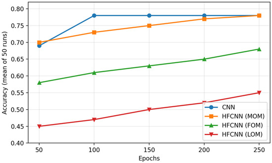
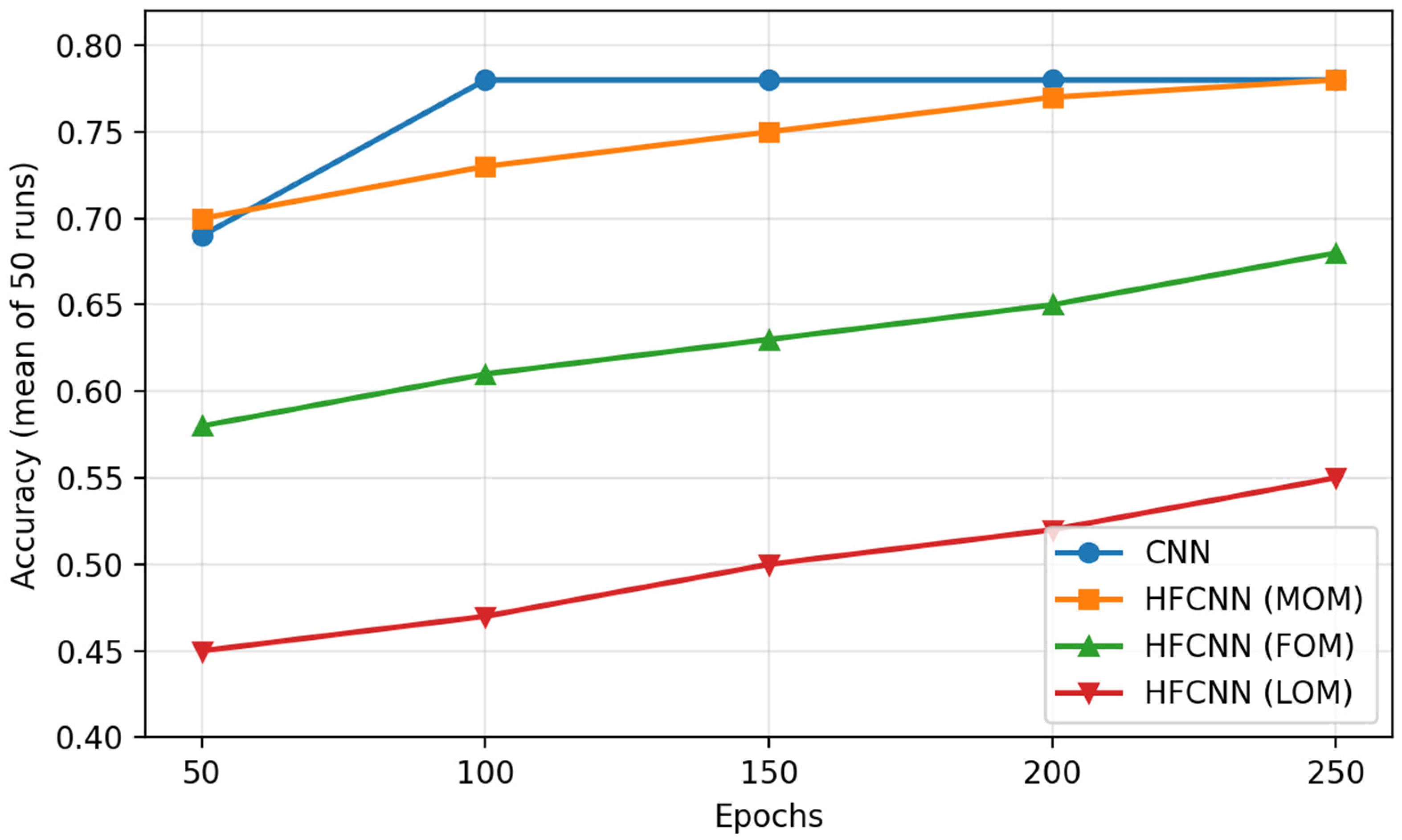
Table 2 presents the results of testing the CNN and HFCNNs using FOM, LOM, and MOM as the defuzzification method. Figure 5 presents mean test accuracy according to the different defuzzification methods.

Table 2. CNN and HFCNN results with different defuzzification methods.

Network	Metric	50 ep.	100 ep.	150 ep.	200 ep.	250 ep.
CNN	Accuracy	0.69	0.78	0.78	0.78	0.78
	Precision	0.69	0.79	0.78	0.79	0.78
	Recall	0.69	0.78	0.79	0.78	0.78
	F1-score	0.68	0.78	0.78	0.78	0.78
HFCNN (FOM)	Accuracy	0.58	0.61	0.63	0.65	0.68
	Precision	0.62	0.63	0.65	0.67	0.69
	Recall	0.57	0.60	0.63	0.66	0.68
	F1-score	0.56	0.59	0.62	0.65	0.67
HFCNN (LOM)	Accuracy	0.45	0.47	0.50	0.52	0.55
	Precision	0.42	0.45	0.47	0.50	0.52
	Recall	0.45	0.48	0.51	0.54	0.55
	F1-score	0.42	0.44	0.46	0.51	0.58
HFCNN (MOM)	Accuracy	0.70	0.73	0.75	0.77	0.78
	Precision	0.71	0.73	0.76	0.78	0.79
	Recall	0.70	0.73	0.75	0.77	0.78
	F1-score	0.70	0.73	0.75	0.77	0.78

Figure 5. Mean test accuracy versus number of training epochs for the CNN and the HFCNN with three defuzzification methods (mean of 50 repetitions).

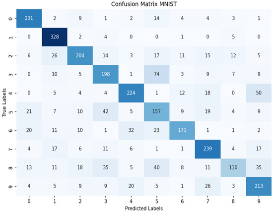
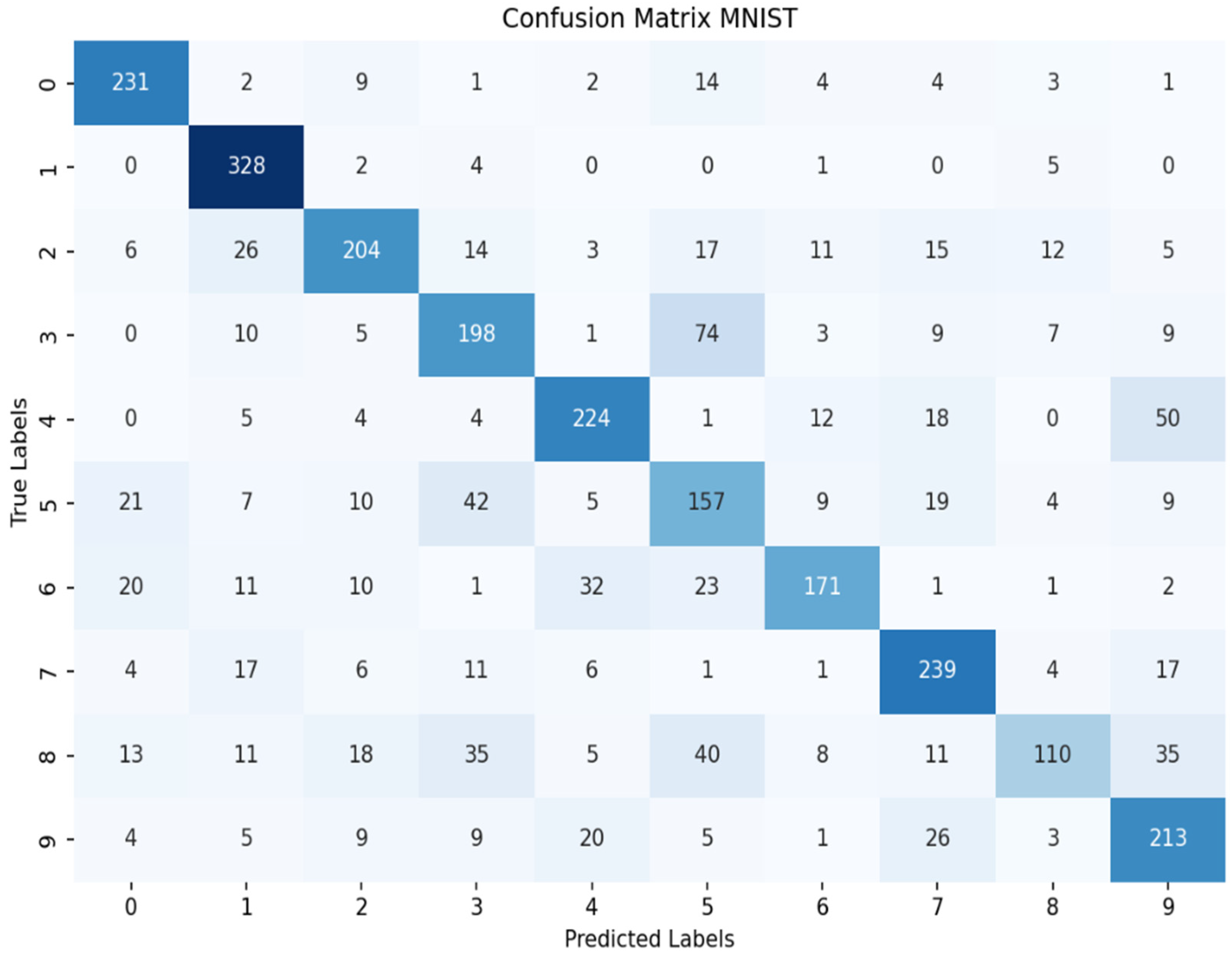
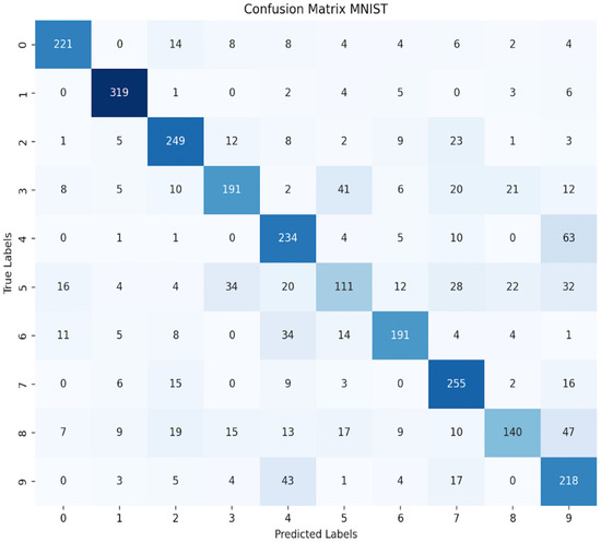
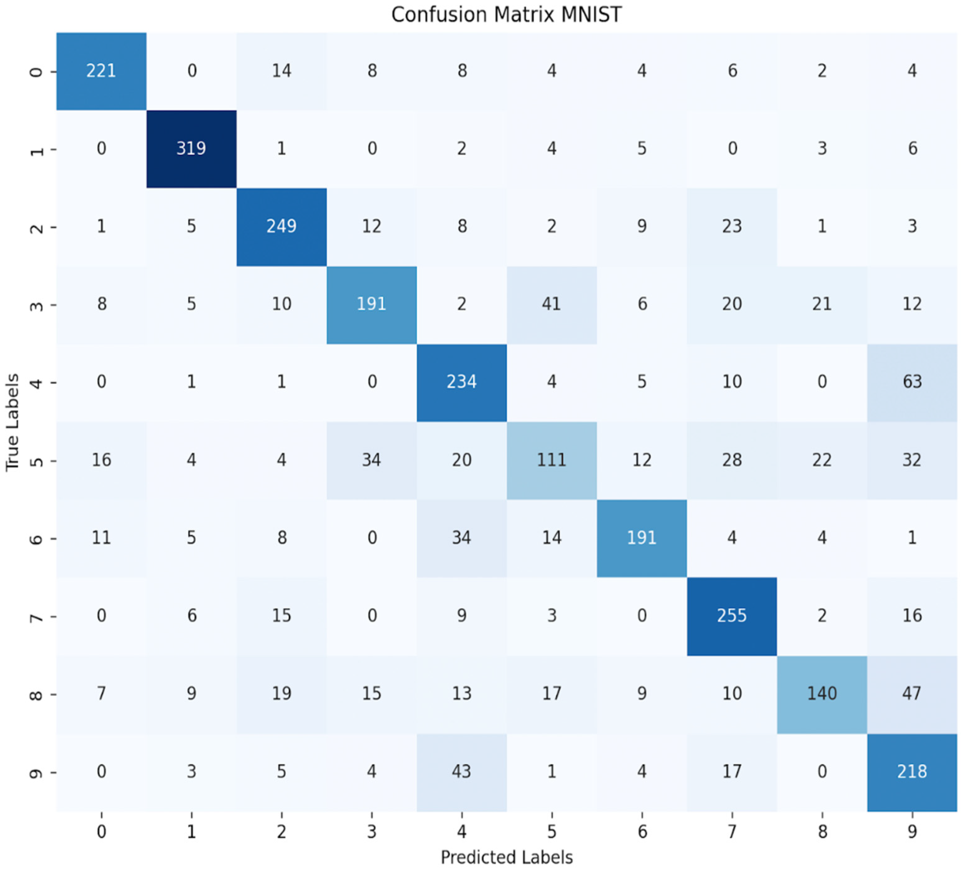
Figure 6 and Figure 7 present the confusion matrices for the CNN and HFCNNs. The tables summarize the average values of the evaluation parameters for the conducted training experiments.

Figure 6. Confusion matrix of CNN with 50 epochs. Color intensity represents the number of samples, where darker blue indicates higher values.

Figure 7. Confusion matrix of HFCNN with 50 epochs. Color intensity represents the number of samples, where darker blue indicates higher values.

Table 3 presents the statistical comparison of CNN, CNND, and HFCNN at 50 epochs, while Table 4 presents the CPU and memory utilization.

Table 3. Comparison of CNN, CNN4, and HFCNN at 50 epochs. Point estimates come from a representative run; 95% confidence intervals were obtained by bootstrap resampling of the test set (5000 replicates, n = 3000); p-values refer to a two-proportion z-test of accuracy against the CNN baseline.

Network	Accuracy	95% CI (Accuracy)	Macro F1	95% CI (Macro F1)	p vs. CNN
CNN	0.6893	[0.673, 0.705]	0.6762	[0.659, 0.692]	—
CNN4	0.7500	[0.734, 0.765]	0.7451	[0.729, 0.760]	<0.001
HFCNN (MOM)	0.6967	[0.679, 0.713]	0.6932	[0.676, 0.709]	0.538
HFCNN (FOM)	0.5370	[0.519, 0.555]	0.5148	[0.497, 0.532]	<0.001

Table 4. Comparison of resident set size (RSS, psutil) and CPU utilization of the CNN, HFCNN (MOM), and CNN4 networks measured at the same stages of program execution, together with the number of trainable parameters of each architecture.

Program Stage	CNN		HFCNN (MOM)		CNN4
	RSS [MB]	CPU [%]	RSS [MB]	CPU [%]	RSS [MB]	CPU [%]
Baseline (before data loading)	487.31	–	463.41	–	506.12	–
After data loading	534.98	12.32	538.66	12.32	575.27	12.32
Before training	535.11	14.95	538.84	13.03	585.28	25.18
After training	459.84	15.05	353.69	13.34	575.27	25.28
After prediction	466.22	15.06	344.78	13.53	567.78	25.37
Trainable parameters	339,160		85,615		≈1,356,460

Results on the ELPV Electroluminescence Benchmark

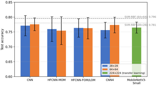
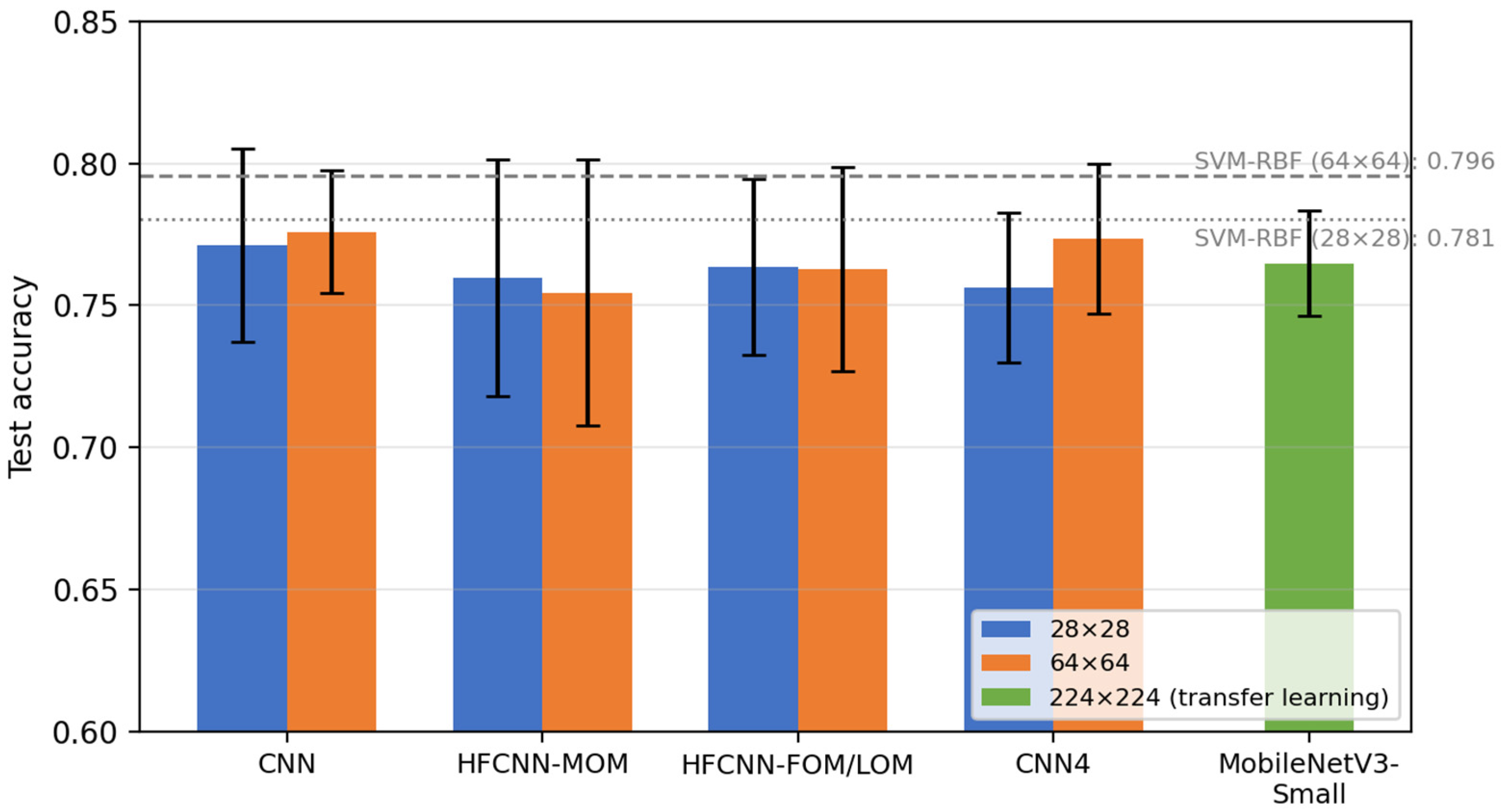
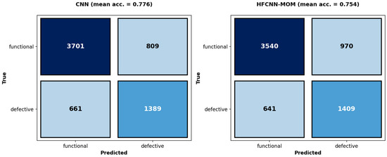
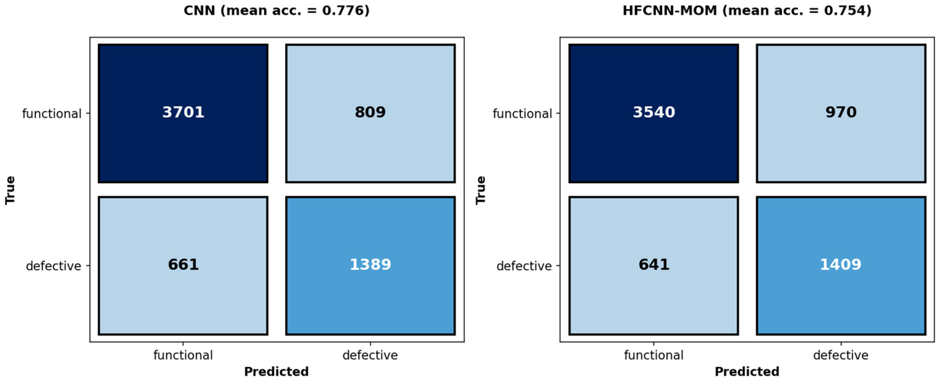
Table 5 and Table 6 summarize the results obtained on the ELPV test set (n = 656) at input resolutions of 28 × 28 and 64 × 64, respectively; Figure 8 compares the mean accuracies, and Figure 9 shows the confusion matrices of the CNN and the HFCNN (MOM) aggregated over the ten runs at 64 × 64. At 28 × 28, the HFCNN with MOM defuzzification reaches 75.99 ± 4.17% accuracy versus 77.13 ± 3.41% for the CNN; the difference of 1.14 percentage points is not statistically significant (Welch’s t-test, p = 0.51). The same picture holds at 64 × 64 (75.44 ± 4.68% vs. 77.59 ± 2.16%, p = 0.20), where the 95% confidence interval of the accuracy difference (−1.1 to +5.4 percentage points) contains zero. The hybrid network thus attains CNN-level accuracy on real electroluminescence imagery while using a dense layer four times smaller and training two to three times faster per epoch. The FOM and LOM variants produced bit-identical results at both resolutions (76.37% at 28 × 28 and 76.28% at 64 × 64), empirically confirming the equivalence derived in Section 4.1. Enlarging the dense layer to 400 neurons (CNN4) did not improve accuracy over the CNN at either resolution despite a four- to sixteen-fold increase in the number of trainable parameters, which is consistent with the MNIST findings.

Table 5. Binary classification of ELPV electroluminescence images at 28 × 28 input resolution: mean ± standard deviation over ten random seeds (50 epochs). Times refer to one training epoch on a single CPU core with the vectorized implementation.

Model	Accuracy	Macro-F1	Trainable Parameters	Time per Epoch [s]
CNN	0.7713 ± 0.0341	0.7430 ± 0.0250	341,727	2.7
HFCNN (MOM)	0.7599 ± 0.0417	0.7310 ± 0.0290	88,158	1.3
HFCNN (FOM = LOM)	0.7637 ± 0.0310	0.7360 ± 0.0190	88,158	1.3
CNN4	0.7561 ± 0.0264	0.7100 ± 0.0320	1,356,627	9.2
Logistic regression	0.7378	0.7103	–	<1
SVM (RBF)	0.7805	0.7466	–	<1
Random forest	0.7759	0.7099	–	<1

Table 6. Binary classification of ELPV electroluminescence images at 64 × 64 input resolution (ten random seeds, 50 epochs). MobileNetV3-Small was fine-tuned at its native 224 × 224 resolution.

Model	Accuracy	Macro-F1	Trainable Parameters	Time per Epoch [s]
CNN	0.7759 ± 0.0216	0.7432 ± 0.0171	1,941,567	16.5
HFCNN (MOM)	0.7544 ± 0.0468	0.7233 ± 0.0355	499,998	6.3
HFCNN (FOM = LOM)	0.7628 ± 0.0358	0.7320 ± 0.0244	499,998	6.4
CNN4	0.7735 ± 0.0265	0.7427 ± 0.0170	7,708,467	62.7
Logistic regression	0.7744	0.7408	–	<1
SVM (RBF)	0.7957	0.7648	–	<1
Random forest	0.7866	0.7188	–	<1
MobileNetV3-Small (224 × 224, TL)	0.7648 ± 0.0185	0.7472 ± 0.0153	939,697	–

Figure 8. Mean test accuracy (±standard deviation over ten seeds) of the compared models on the ELPV benchmark at 28 × 28 and 64 × 64 input resolution; dashed lines mark the SVM-RBF baselines.

Figure 9. Confusion matrices of the CNN and the HFCNN (MOM) on the ELPV test set at 64 × 64, aggregated over ten random seeds. Color intensity represents the number of samples, where darker blue indicates higher values.

The classical baselines put these numbers into perspective. The SVM with RBF kernel achieved the highest accuracy overall (78.05% at 28 × 28 and 79.57% at 64 × 64), and the fine-tuned MobileNetV3-Small reached 76.48 ± 1.85%—comparable to the networks trained from scratch, but not superior to the SVM at these settings. This indicates that binary crack detection on strongly downscaled EL images is largely a texture-contrast problem that classical kernels capture well; the added value of convolutional models, including the proposed hybrid, is expected to grow for finer-grained defect taxonomies and higher input resolutions, as reported in Ref. [4] for full-resolution transfer learning with data augmentation (88.4%). Within the scope of this study, the ELPV experiments confirm the central methodological claim: the OFN-based dense layer preserves the classification quality of its crisp counterpart at a substantially lower parametric and computational cost.

6. Discussion

The performance of the HFCNN using LOM for defuzzification was the worst. Using FOM improved HFCNN results compared to LOM, but they were still lower than those of the CNN. The use of MOM defuzzification allowed HFCNN to achieve slightly better prediction results than CNN, despite having a much smaller deep layer—only 25% the size of the corresponding layer in the CNN.

In some cases, the image recognition improvement for HFCNN with MOM defuzzification reached up to 8%. Increasing the number of training epochs improved prediction quality; however, enlarging the CNN did not lead to a significant increase in image recognition accuracy.

The difference between HFCNN (MOM) and the CNN baseline is not statistically significant (p = 0.538), which supports the central claim of the paper—the hybrid network reaches CNN-level quality with a dense layer four times smaller (25 vs. 100 neurons). CNN4 is significantly better than both (p < 0.001), which is expected given its 4× larger dense layer, and FOM is significantly worse.

Table 7 summarizes the computational footprint of the three architectures. The proposed HFCNN has 85,615 trainable parameters—approximately four times fewer than the baseline CNN (339,160) and sixteen times fewer than CNN4 (1,356,460)—even though each weight of its fuzzy output layer is an Ordered Fuzzy Number represented by four values. This reduction is reflected in the runtime measurements (Table 4): during training and prediction, the HFCNN exhibits the lowest CPU utilization (≈13–13.5%, compared with ≈15% for the CNN and ≈25% for CNN4) and the smallest memory footprint after training (≈345–354 MB RSS, versus ≈460–466 MB for the CNN and ≈568–585 MB for CNN4). Combined with the statistical analysis of the classification results, which showed comparable accuracy between the HFCNN with MOM defuzzification and the CNN baseline at 50 epochs (p = 0.538), these measurements demonstrate that the proposed hybrid architecture attains CNN-level classification quality at a substantially lower computational cost. CNN4, in turn, achieves significantly higher accuracy, but at the price of a sixteen-fold increase in the number of parameters and roughly twice the CPU load relative to the HFCNN, which makes the hybrid network an attractive trade-off for resource-constrained applications.

Table 7. Number of trainable parameters per layer.

Layer	CNN	HFCNN (MOM)	CNN4
Convolutional (3 × 3, depth 5)	50	50	50
Dense (3380 → h)	338,100 (h = 100)	84,525 (h = 25)	1,352,400 (h = 400)
Output layer (h → 10)	1010 (Dense)	1040 (DenseOFN, 4 values per weight)	4010 (Dense)
Total	339,160	85,615	1,356,460

A straightforward implementation of this architecture requires an OFN class together with operators for the arithmetic of Ordered Fuzzy Numbers [48]. Such an object-oriented implementation, however, is effectively CPU-bound: modern AI workflows rely on graphics processing units (GPUs), and a class-based representation is difficult to map onto the vectorized primitives available in GPU libraries.

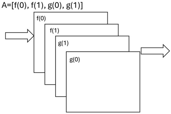
For this reason, a second implementation is under development. Because multiplication, division, addition, and subtraction of OFNs operate on four component values and there is no interference between components during these operations, the class can be avoided altogether. Instead, the four components f(0), f(1), g(0), g(1) of each OFN are stored as four separate arrays of equal shape, and the arithmetic is performed element-wise on these four arrays. The resulting data layout is illustrated in Figure 10.

Figure 10. Array-based representation of Ordered Fuzzy Numbers used in the GPU-oriented implementation: each OFN A = [f(0), f(1), g(0), g(1)] is decomposed into four aligned arrays.

This representation allowed the network to be implemented with the CuPy library, which made it possible to accelerate the learning process. It will also allow moving computations from the CPU to the GPU in the future. The price to pay is a larger number of auxiliary arrays and a corresponding modification of the training and prediction algorithms; the gain is a very substantial speed-up of the computations, reported in Section 5. The first implementation requires 19 min and 52 s for a single epoch. The modification of the code allowed us to use the PV dataset and test the proposed solutions against other methods.

The HFCNN architecture is particularly suited for PV applications because it naturally handles measurement uncertainty and environmental variability through fuzzy logic mechanisms. Photovoltaic panel monitoring inherently involves uncertain measurements due to cloud transients, temperature fluctuations, and sensor limitations. The fuzzy logic mechanisms in HFCNN provide natural representations of this uncertainty, enabling more robust anomaly detection compared to crisp classification methods. Furthermore, the reduced computational complexity enables deployment on edge computing devices at PV installation sites, eliminating the need for continuous cloud connectivity and enabling real-time autonomous decision-making.

The Hybrid Fuzzy Convolutional Neural Network architecture presents significant opportunities for future application in photovoltaic system monitoring and energy optimization. The experimental results demonstrate that HFCNN achieves comparable or superior performance to traditional CNNs while reducing computational requirements by 75%. This substantial reduction in network parameters enables deployment of sophisticated anomaly detection capabilities on edge computing devices at individual PV installation sites.

Key applications include the following: (1) Thermal anomaly detection in photovoltaic panels—identifying hotspots indicating cell degradation or failure using infrared imaging [24]; (2) Visual defect detection—recognizing physical damage, soiling, or contamination on panel surfaces; (3) Performance state classification—distinguishing between normal operation, partial degradation, and complete failure states to support maintenance scheduling; (4) Multi-modal fusion—integrating visual and thermal data for comprehensive system health monitoring; (5) Real-time decision support—enabling autonomous switching between operational modes or triggering maintenance alerts based on detected anomalies.

The ELPV experiments (Section Results on the ELPV Electroluminescence Benchmark) transfer the MNIST conclusions to real photovoltaic imagery. On electroluminescence images of solar cells, the HFCNN with MOM defuzzification is statistically indistinguishable from the CNN baseline at both tested resolutions (p = 0.51 and p = 0.20), while its dense layer is four times smaller and one training epoch is two to three times faster; CNN4 again offers no accuracy gain despite up to sixteen times more parameters. The bit-exact equality of the FOM and LOM variants observed on ELPV empirically confirms the equivalence derived in Section 4.1 and turns the earlier empirical observation that MOM is the preferable operator into a result with a theoretical explanation: under the uniform update rule, the effective FOM/LOM weights equal the MOM weights shifted by a frozen, non-negative random offset.

An honest reading of Table 6 also shows the limits of the present setting: the SVM with RBF kernel remains the strongest model on the binary ELPV task, and the fine-tuned MobileNetV3-Small does not surpass it either. Binary crack detection on downscaled EL images therefore does not, by itself, require deep feature hierarchies; the practical case for the proposed hybrid lies in scenarios where a resource-efficient network trainable from scratch is preferred—for example, embedded inspection devices—and in more demanding, multi-class defect taxonomies, for which the fuzzy representation of uncertainty is expected to be most useful. These scenarios define the next experimental step.

The efficiency concern raised by the object-oriented implementation has meanwhile been resolved on the CPU. The array-based representation of Figure 10 was implemented directly in NumPy; the vectorized layer is numerically identical to the object-oriented one, while a single training epoch of the deep profiling stack used for the runtime measurements dropped from approximately 3.5 h to 109 s on one CPU core—a speed-up of about two orders of magnitude (≈118×). For the compact HFCNN of Table 1, one epoch on the full ELPV training set takes about 1.3 s at 28 × 28 and 6.3 s at 64 × 64. Since the four-component representation maps directly onto GPU array libraries, the same code path can be executed with CuPy.

7. Conclusions

This work presented the Hybrid Fuzzy Convolutional Neural Network (HFCNNs)—to the best of the authors’ knowledge, the first integration of Ordered Fuzzy Numbers into a convolutional neural network architecture. The proposed Dense Fuzzy Layer operates entirely in OFN arithmetic and, unlike classical fuzzy systems such as ANFIS, does not require expert-designed membership functions: the fuzzy representations are learned end-to-end through standard backpropagation, and the network can be used as easily as a conventional model defined in frameworks such as TensorFlow or PyTorch.

The experimental results on the MNIST dataset support three main findings. First, the HFCNN with Mean of Maxima (MOM) defuzzification achieved classification quality statistically indistinguishable from the baseline CNN (p = 0.538), despite using a dense layer four times smaller (25 vs. 100 neurons). Second, this parameter efficiency translates into concrete resource savings: 85,615 trainable parameters versus 339,160 for the CNN (a 75% reduction), the lowest CPU utilization of the three tested architectures (≈13% vs. ≈15% for CNN and ≈25% for CNN4), and the smallest memory footprint (≈350 MB vs. ≈460 MB and ≈580 MB, respectively). Third, the choice of defuzzification operator proved critical: MOM clearly outperformed FOM and LOM, indicating that operators accounting for both slopes of an Ordered Fuzzy Number are better suited for classification tasks.

A smaller architecture with comparable accuracy implies lower hardware requirements, making it possible to run recognition tasks on lower-class processors or to extend the operational time of battery-powered systems—properties that are particularly attractive for edge computing devices at distributed photovoltaic installations.

Several limitations of the present study must be acknowledged. The validation was performed on a reduced MNIST subset rather than on real photovoltaic imagery; therefore, this work constitutes a methodological contribution, and no claims about practical PV deployment readiness can be made at this stage. The current CPU-bound, object-oriented implementation limits the scale of the experiments; the array-based GPU implementation using the CuPy library, described in Section 6, is under development and will enable training on the full MNIST dataset and larger benchmarks. Finally, the evaluation covered a single, relatively shallow convolutional backbone.

Future research will focus on (1) validation with actual PV thermal and visual imagery datasets, including comparison with expert analysis of thermographic images; (2) scaling the GPU implementation to full benchmark datasets and deeper backbones such as ResNet; (3) investigation of multi-modal fusion combining thermal and visual inputs; (4) systematic analysis of further defuzzification operators that exploit the orientation of Ordered Fuzzy Numbers; (5) deployment and performance evaluation on edge computing devices at actual PV installations; and (6) integration with predictive maintenance models and interpretable decision support systems for system operators.

The present revision adds the validation that the original submission lacked: the architecture was evaluated on 2624 real electroluminescence images of photovoltaic cells from the public ELPV benchmark, with a ten-seed statistical protocol, classical machine-learning baselines, and a lightweight transfer-learning reference. The central claim was confirmed on real PV data—the HFCNN with MOM defuzzification matches the CNN baseline within statistical uncertainty at both tested resolutions while using a four times smaller dense layer—and the equivalence of the FOM and LOM operators under the adopted initialization was both derived analytically and observed empirically. At the same time, the experiments delimit the claim honestly: on the binary ELPV task, an SVM with RBF kernel remains slightly stronger than all evaluated neural models, so the practical advantage of the hybrid architecture should be sought in resource-constrained deployments and in finer-grained defect classification.

References

- Osowski, S. Głębokie sieci neuronowe i ich zastosowania w eksploracji danych. Przegląd Telekomun.-Wiad. Telekomun. 2018, 2018, 112–121. [Google Scholar]
- Stanford University. Improved Anomaly Detection Using Adversarially Learned Inference. Docket #S19-208, 2019. Available online: https://techfinder.stanford.edu/print/pdf/node/30748 (accessed on 10 August 2024).
- Brabec, C.J.; Camus, C.; Hauch, J.; Doll, B.; Berger, S.; Gallwitz, F.; Maier, A.; Deitsch, S.; Buerhop-Lutz, C. A Benchmark for Visual Identification of Defective Solar Cells in Electroluminescence Imagery. In Proceedings of the World Conference on Photovoltaic Energy Conversion, Brussels, Belgium, 6 November 2018; pp. 1287–1289. [Google Scholar] [CrossRef]
- Deitsch, S.; Buerhop-Lutz, C.; Sovetkin, E.; Steland, A.; Maier, A.; Gallwitz, F.; Riess, C. Automatic classification of defective photovoltaic module cells in electroluminescence images. Sol. Energy 2019, 185, 455–468. [Google Scholar] [CrossRef] [Scilit]
- Howard, A.; Sandler, M.; Chu, G.; Chen, L.-C.; Chen, B.; Tan, M.; Wang, W.; Zhu, Y.; Pang, R.; Vasudevan, V.; et al. Searching for MobileNetV3. In Proceedings of the IEEE/CVF International Conference on Computer Vision (ICCV), Seoul, Republic of Korea, 27 October–2 November 2019; pp. 1314–1324. [Google Scholar]
- Zhao, X.; Wang, L.; Zhang, Y.; Han, X.; Deveci, M.; Parmar, M. A review of convolutional neural networks in computer vision. Artif. Intell. Rev. 2024, 57, 99. [Google Scholar] [CrossRef] [Scilit]
- Chen, F.; Li, S.; Han, J.; Ren, F.; Yang, Z. Review of Lightweight Deep Convolutional Neural Networks. Arch. Comput. Methods Eng. 2024, 31, 1915–1937. [Google Scholar] [CrossRef] [Scilit]
- Raiaan, M.A.K.; Sakib, S.; Fahad, N.M.; Mamun, A.A.; Rahman, M.A.; Shatabda, S.; Mukta, M.S.H. A systematic review of hyperparameter optimization techniques in Convolutional Neural Networks. Decis. Anal. J. 2024, 11, 100470. [Google Scholar] [CrossRef] [Scilit]
- Hasan, M.A.; Bhargav, T.; Sandeep, V.; Reddy, V.S.; Ajay, R. Image classification using convolutional neural networks. Int. J. Mech. Eng. Res. Technol. 2024, 16, 173–181. [Google Scholar]
- Wang, C.; Wang, X.; Wu, D.; Kuang, M.; Li, Z. Meticulous Land Cover Classification of High-Resolution Images Based on Interval Type-2 Fuzzy Neural Network with Gaussian Regression Model. Remote Sens. 2022, 14, 3704. [Google Scholar] [CrossRef] [Scilit]
- Wang, Y.; Ishibuchi, H.; Er, M.J.; Zhu, J. Unsupervised multilayer fuzzy neural networks for image clustering. Inf. Sci. 2023, 622, 682–709. [Google Scholar] [CrossRef] [Scilit]
- Wang, C.; Lv, X.; Shao, M.; Qian, Y.; Zhang, Y. A novel fuzzy hierarchical fusion attention convolution neural network for medical image super-resolution reconstruction. Inf. Sci. 2023, 622, 424–436. [Google Scholar] [CrossRef] [Scilit]
- Mittal, N.; Vaidya, A.; Kapoor, S. Object detection and classification using Yolo. Int. J. Sci. Res. Eng. Trends 2019, 5, 871–875. [Google Scholar]
- Diwan, T.; Anirudh, G.; Tembhurne, J.V. Object detection using YOLO: Challenges, architectural successors, datasets and applications. Multimed. Tools Appl. 2023, 82, 9243–9275. [Google Scholar] [CrossRef] [Scilit] [PubMed]
- Wang, S.; Niu, L.; Li, N. Research on image recognition of insulators based on YOLO algorithm. In 2018 International Conference on Power System Technology (POWERCON); IEEE: New York, NY, USA, 2018; pp. 3871–3874. [Google Scholar]
- Guan, Z. Real-time object recognition based on YOLO model. Theor. Nat. Sci. 2023, 28, 137–143. [Google Scholar] [CrossRef] [Scilit]
- Hendry; Chen, R.C. Automatic License Plate Recognition via sliding-window darknet-YOLO deep learning. Image Vis. Comput. 2019, 87, 47–56. [Google Scholar] [CrossRef] [Scilit]
- Lin, J.P.; Sun, M.T. A YOLO-based traffic counting system. In 2018 Conference on Technologies and Applications of Artificial Intelligence (TAAI); IEEE: New York, NY, USA, 2018; pp. 82–85. [Google Scholar]
- Matsuhashi, S.; Sugiura, R.; Asai, M.; Asami, H.; Kowata, Y.; Akamatsu, Y.; Sasaki, K.; Yoshino, N.; Ihara, N.; Koarai, A. Field evaluation of an agricultural weed detector using YOLO image recognition: Background conditions affect detection performance. Pest Manag. Sci. 2025, 81, 6560–6566. [Google Scholar] [CrossRef] [Scilit] [PubMed]
- Available online: https://docs.ultralytics.com/ (accessed on 5 October 2025).
- Magdin, M.; Balogh, Z. Comparison classification algorithms and the YOLO method for video analysis and object detection. Sci. Rep. 2025, 15, 25432. [Google Scholar] [CrossRef] [Scilit] [PubMed]
- Jorge, V.L.; Bendaoud, I.; Soulié, F.; Bordreuil, C. Deep learning-based YOLO for semantic segmentation and classification of weld pool thermal images. Int. J. Adv. Manuf. Technol. 2025, 137, 3573–3585. [Google Scholar] [CrossRef] [Scilit]
- Alruwaili, M.; Mohamed, M. An Integrated Deep Learning Model with EfficientNet and ResNet for Accurate Multi-Class Skin Disease Classification. Diagnostics 2025, 15, 551. [Google Scholar] [CrossRef] [Scilit] [PubMed]
- Wu, W.; Huo, L.; Yang, G.; Liu, X.; Li, H. Research into the Application of ResNet in Soil: A Review. Agriculture 2025, 15, 661. [Google Scholar] [CrossRef] [Scilit]
- Bhardwaj, D.; Nagabhooshanam, N.; Singh, A.; Selvalakshmi, B.; Angadi, S.; Shargunam, S.; Guha, T.; Singh, G.; Rajaram, A. Enhanced satellite imagery analysis for post-disaster building damage assessment using integrated ResNet-U-Net model. Multimed. Tools Appl. 2025, 84, 2689–2714. [Google Scholar] [CrossRef] [Scilit]
- Wang, X.; Dai, J.; Liu, X. A spatial-temporal neural network based on ResNet-Transformer for predicting railroad broken rails. Adv. Eng. Inform. 2025, 65, 103126. [Google Scholar] [CrossRef] [Scilit]
- Shu, Y.; Zhang, J.; Wang, Y.; Wei, Y. Fruit Freshness Classification and Detection Based on the ResNet-101 Network and Non-Local Attention Mechanism. Foods 2025, 14, 1987. [Google Scholar] [CrossRef] [Scilit] [PubMed]
- Li, L.; Wang, R.; Zou, M.; Guo, F.; Ren, Y. Enhanced ResNet-50 for garbage classification: Feature fusion and depth-separable convolutions. PLoS ONE 2025, 20, e0317999. [Google Scholar] [CrossRef] [Scilit] [PubMed]
- Mjahad, A.; Rosado-Muñoz, A. Hybrid CNN-Fuzzy Approach for Automatic Identification of Ventricular Fibrillation and Tachycardia. Appl. Sci. 2025, 15, 9289. [Google Scholar] [CrossRef] [Scilit]
- Mahmud, A.; Shishir, M.S.R.; Hasan, R.; Rahman, M. A comprehensive study for solar panel fault detection using VGG16 and VGG19 convolutional neural networks. In Proceedings of the 2023 26th International Conference on Computer and Information Technology (ICCIT), Cox’s Bazar, Bangladesh, 13–15 December 2023; pp. 1–6. [Google Scholar] [CrossRef] [Scilit]
- Sabati, A.; Bayindir, R.; Rahebi, J. Photovoltaic Panels Fault Detection with Convolutional Neural Network and Bitterling Fish Optimization (BFO) Algorithm. Int. J. Comput. Intell. Syst. 2025, 18, 239. [Google Scholar] [CrossRef] [Scilit]
- Appavu, N. AI Deep VGG19-based Heatmap Analysis and Thermal Imaging for Photovoltaic Panel Fault Detection. In Proceedings of the 2025 6th International Conference on Electronics and Sustainable Communication Systems (ICESC), Coimbatore, India, 10–12 September 2025; pp. 1572–1577. [Google Scholar] [CrossRef] [Scilit]
- Jia, Y.; Chen, G.; Zhao, L. Defect detection of photovoltaic modules based on improved VarifocalNet. Sci. Rep. 2024, 14, 15170. [Google Scholar] [CrossRef] [Scilit] [PubMed]
- Abdelsattar, M.; AbdelMoety, A.; Emad-Eldeen, A. ResNet-based image processing approach for precise detection of cracks in photovoltaic panels. Sci. Rep. 2025, 15, 24356. [Google Scholar] [CrossRef] [Scilit] [PubMed]
- Shin, M.; Seo, J.; Lee, I.-B.; Kim, S. Defective Photovoltaic Module Detection Using EfficientNet-B0 in the Machine Vision Environment. Machines 2026, 14, 232. [Google Scholar] [CrossRef] [Scilit]
- Yang, X.; Li, Y.; Yang, L.; Zhang, Y.; Wang, X.; Zhang, Q. High-noise solar panel defect identification method based on the improved EfficientNet-V2. J. Renew. Sustain. Energy 2024, 16, 053704. [Google Scholar] [CrossRef] [Scilit]
- Zhang, J.; Yang, W.; Chen, Y.; Ding, M.; Huang, H.; Wang, B.; Gao, K.; Chen, S.; Du, R. Fast object detection of anomaly photovoltaic (PV) cells using deep neural networks. Appl. Energy 2024, 372, 123759. [Google Scholar] [CrossRef] [Scilit]
- Khanam, R.; Hussain, M. YOLOv11: An overview of the key architectural enhancements. arXiv 2024, arXiv:2410.17725. [Google Scholar]
- Qader, M.R.; Albalooshi, F.A. Boosting Solar Panel Reliability: An Attention-Enhanced Deep Learning Model for Anomaly Detection. Energies 2025, 18, 6591. [Google Scholar] [CrossRef] [Scilit]
- Su, B.; Zhou, Z.; Chen, H. PVEL-AD: A Large-Scale Open-World Dataset for Photovoltaic Cell Anomaly Detection. IEEE Trans. Ind. Inform. 2023, 19, 404–413. [Google Scholar] [CrossRef] [Scilit]
- Lai, Y.-S.; Hsieh, C.-C.; Liao, T.-W.; Huang, C.-Y.; Kuo, C.-F.J. Deep learning-based automatic defect detection of photovoltaic modules in infrared, electroluminescence, and red–green–blue images. Energy Convers. Manag. 2025, 332, 119783. [Google Scholar] [CrossRef] [Scilit]
- Apiecionek, L. Fuzzy Neural Networks—A Review with Case Study. Appl. Sci. 2025, 15, 6980. [Google Scholar] [CrossRef] [Scilit]
- Lin, C.T.; Lee, C.G. Neural-network-based fuzzy logic control and decision system. IEEE Trans. Comput. 1991, 40, 1320–1336. [Google Scholar] [CrossRef] [Scilit]
- Chow, M.Y. Methodologies of Using Artificial Neural Network and Fuzzy Logic Technologies for Motor Incipient Fault Detection; World Scientific: Singapore, 1997. [Google Scholar]
- Goode, P.; Chow, M.Y. Using a neural/fuzzy system to extract knowledge of incipient fault in induction motors part I—Methodology. IEEE Trans. Ind. Electron. 1995, 42, 131–138. [Google Scholar] [CrossRef] [Scilit]
- Jang, J.-S.; Sun, C.-T.; Mizutani, E. Neuro-Fuzzy and Soft Computing—A Computational Approach to Learning and Machine Intelligence; Prentice Hall Intern. Inc.: Upper Saddle River, NY, USA, 1997. [Google Scholar]
- Available online: https://github.com/jfpower/anfis-pytorch/blob/master/iris_example.py (accessed on 8 February 2025).
- Prokopowicz, P.; Czerniak, J.; Mikołajewski, D.; Apiecionek, Ł.; Ślȩzak, D. (Eds.) Theory and Applications of Ordered Fuzzy Numbers: A Tribute to Professor Witold Kosiński; Springer: Cham, Switzerland, 2017. [Google Scholar] [CrossRef] [Scilit]
- Pedregosa, F.; Varoquaux, G.; Gramfort, A.; Michel, V.; Thirion, B.; Grisel, O.; Blondel, M.; Prettenhofer, P.; Weiss, R.; Dubourg, V.; et al. Scikit-learn: Machine Learning in Python. J. Mach. Learn. Res. 2011, 12, 2825–2830. [Google Scholar]
Disclaimer/Publisher’s Note: The statements, opinions and data contained in all publications are solely those of the individual author(s) and contributor(s) and not of MDPI and/or the editor(s). MDPI and/or the editor(s) disclaim responsibility for any injury to people or property resulting from any ideas, methods, instructions or products referred to in the content. |
© 2026 by the author. Licensee MDPI, Basel, Switzerland. This article is an open access article distributed under the terms and conditions of the Creative Commons Attribution (CC BY) license.