


Abstract
Continuous carbon anode roasting in industrial parks requires a stable high-temperature heat supply and remains highly dependent on grid electricity and natural gas. However, existing energy-system studies rarely coordinate hydrogen production and storage, volumetric hydrogen blending, and temperature-graded waste-heat recovery under continuous production constraints. To address this gap, this study proposes an electricity–heat–gas–hydrogen integrated energy system for carbon anode industrial parks and develops a 24 h multi-objective scheduling model. The model coordinates heat demands at different temperature levels with hourly electricity and hydrogen flows, using surplus photovoltaic power to produce hydrogen for later high-load periods. The selected scheme achieves a daily volumetric hydrogen-blending ratio of 10.79%, with an operating cost of 82,985.75 CNY and carbon emissions of 54,371.53 kg. Relative to an otherwise equivalent non-hydrogen configuration, hydrogen coupling provides additional reductions of 7.2% in operating cost and 2.3% in carbon emissions. Compared with a basic conventional configuration, operating cost and carbon emissions decrease by 27.9% and 26.0%, respectively. Cascade recovery also increases the daily waste-heat utilization rate by approximately 30 percentage points. These results show that the proposed scheduling framework can coordinate hydrogen utilization and graded waste-heat recovery while maintaining continuous carbon anode production.
1. Introduction
China’s carbon-neutrality commitment has increased the need to reduce fossil-fuel use and carbon emissions in energy-intensive industries. Continuous high-temperature processes face stricter operating constraints. Stable production requires a continuous thermal energy supply. This limits the flexibility for load interruption or fuel substitution [1]. The low-carbon transition is especially difficult for continuous energy-intensive processes, where process stability and emission reduction are tightly coupled. Carbon anode production for aluminum electrolysis is a representative case, with high energy consumption, large carbon emissions, and rigid thermal demand during continuous roasting [2,3]. The continuous carbon anode roasting process must maintain a stable energy supply while meeting emission–reduction requirements. The rigid heat demand, high carbon-emission intensity, and potential for high-temperature waste-heat recovery in continuous carbon anode roasting make carbon anode production a relevant application for low-carbon integrated energy system (IES) retrofits. The low-carbon economic viability of IES in carbon anode industrial parks is constrained by two coupling factors. Specifically, insufficient matching precision between waste-heat grades and process temperature requirements leads to the downgraded utilization of high-quality thermal energy, resulting in low overall system efficiency [4,5]. In parallel, increasing the volumetric hydrogen-blending ratio reduces the volume-weighted lower heating value of the blended fuel. Under a fixed furnace heat demand, this change increases the required volumetric fuel flow and alters the hourly allocation of natural gas and hydrogen, thereby complicating coordinated system scheduling [6]. For carbon anode industrial parks, the key challenge is to ensure a stable energy supply for continuous high-temperature roasting. Meanwhile, waste-heat cascade utilization and low-carbon fuel substitution must be coordinated within a unified scheduling framework. Addressing this challenge by elucidating the deep coupling mechanisms of electricity, heat, and hydrogen flows holds clear theoretical and engineering significance [7].
Hydrogen-blended combustion coupled with Power-to-Hydrogen (P2H) is a transitional option for reducing fossil-fuel use in energy-intensive industries. Earlier studies focused on fuel properties and combustion boundaries, reporting changes in flame propagation and combustion stability with hydrogen addition [8,9]. Recent work has extended this topic to system operation. A quasi-steady state scheduling model was developed for a hydrogen-blended electricity–gas system considering gas linepack [10]. Variable-ratio blending of hydrogen with natural gas was included in the capacity configuration of a virtual power plant [11]. Dynamic hydrogen blending was also considered in low-carbon IES scheduling to represent changes in gas composition and calorific value [12]. These studies provide useful references for modeling hydrogen blending at the system level. However, they mainly address electricity–gas networks, virtual power plants, or hydrogen-blended gas turbines. However, these models do not represent continuous carbon anode roasting. In this process, photovoltaic (PV) power, P2H, hydrogen storage, furnace heat demand, and waste heat recovery must be coordinated. Practical blending limits may also depend on burner configuration and operating conditions and therefore require equipment-level verification [13]. In continuous roasting, variations in PV output can alter hourly hydrogen availability and the volumetric blending ratio, thereby affecting the fuel supply required to meet furnace heat demand. Neglecting this coupling may obscure the trade-off among continuous thermal supply, operating cost, and carbon emissions [14]. Accordingly, this study develops a system-level scheduling model that optimizes the hourly hydrogen-blending ratio under the continuous operating constraints of carbon anode roasting.
Parallel to fuel substitution, waste-heat cascade utilization constitutes a critical pathway for the deep decarbonization of IES [15]. While high-temperature waste-heat recovery in industrial kilns has been widely explored, existing technologies generally suffer from poor structural matching [16,17]. In carbon anode roasting, high-temperature flue gas is often either directly emitted or used only for single-grade heating, resulting in a severe mismatch between heat-source temperatures and end-use thermal demands [18]. Resolving this thermodynamic mismatch necessitates the establishment of a cascade utilization architecture tailored to multiple temperature zones, enabling the sequential extraction of usable thermal energy based on temperature gradients [19,20]. However, coupling the hydrogen-blended combustion process with complex waste-heat networks significantly intensifies system nonlinearity, presenting dual challenges of heavy computational burdens and exacerbated objective conflicts in multi-objective optimization. Within the framework of multi-objective optimization, the ε-constraint method exhibits significant precision advantages over traditional weighted sum methods in generating a uniform and non-dominated Pareto front [21]. Furthermore, TOPSIS can be used to rank multi-objective solutions according to specified preference weights [22].
Recent studies have extended low-carbon IES scheduling to multi-objective optimization and decision-making [23,24,25], while industrial applications increasingly consider hydrogen blending and carbon trading [26]. However, coordinated modeling of multi-objective optimization, hydrogen blending, carbon trading, and graded waste-heat recovery under continuous carbon anode production constraints remains limited. To provide a focused comparison, representative peer-reviewed studies were identified through a structured search of the Web of Science Core Collection using keywords related to IESs, hydrogen blending, waste heat, carbon trading, and multi-objective optimization. Titles, abstracts, and full texts were screened manually for methodological relevance and sufficient model detail. Based on these criteria, Table 1 compares the application scope and modeled features of the selected studies.
Table 1.
Comparison of representative low-carbon IES optimization studies and the present study.
Table 1 groups the selected studies into three broad research directions. Representative hydrogen-oriented IES studies model hydrogen blending, storage, or carbon trading, but do not simultaneously represent temperature-graded waste-heat utilization and continuous industrial production [26,27,28]. Studies centered on waste-heat recovery or cascade utilization improve heat-grade matching, but generally exclude dynamic hydrogen production, storage, and fuel substitution [4,29,30]. Industrial-park and multi-objective studies mainly address generic energy coordination, operational scheduling, or capacity planning, with limited representation of hourly fuel composition and process-specific heat grades [22,29,31]. Taken together, these comparisons indicate that the research gap lies not in any individual technology, but in the coordinated representation of these mechanisms within a process-specific scheduling model for continuous carbon anode production.
To address this gap, this study develops a 24 h multi-objective scheduling model for a carbon anode industrial park. The model jointly represents P2H-based hydrogen production and storage, volumetric hydrogen blending in the roasting furnace, stepped carbon trading, and temperature-graded waste-heat utilization. Its main distinction lies in coordinating fuel substitution, intertemporal electricity–hydrogen shifting, and heat-grade matching within the same operational framework.
Figure 1 presents the research workflow from model formulation to result evaluation. The modeling side defines the system inputs and boundaries and then establishes the multi-energy coupled architecture, optimization objectives and comparative cases. The optimization and results side applies the ε-constraint method and TOPSIS to obtain the preferred operating scheme and evaluates the corresponding changes in operating cost, carbon emissions, and waste-heat utilization.
Figure 1.
Comprehensive research framework for the low-carbon transition of carbon anode industrial parks. Note in the picture: pp = percentage points.
2. Methodology
2.1. System Description
Figure 2 presents the physical architecture of the IES for the carbon anode industrial park. The system comprises coupled electricity, heat, gas, and hydrogen networks, supplied by the external power grid, the natural gas network, and distributed PV. Electrical demand represents the main production loads, while thermal demand is divided into high-, medium-, and low-temperature levels. P2H, battery and hydrogen storage, hydrogen-blended combustion, and cascade waste-heat utilization connect the energy carriers and define the physical boundaries of the subsequent multi-objective dispatch model.
Figure 2.
Diagram of multi-energy flows coupled within electricity–heat–gas–hydrogen IES.
Conventional carbon anode industrial parks rely mainly on grid electricity and natural gas combustion. In addition, high-temperature flue gas from continuous roasting is often discharged or recovered at a single temperature level. This operating structure limits coordination among energy supply, conversion, storage, and demand. By linking the four energy networks through the conversion and storage equipment shown in Figure 2, the proposed configuration coordinates electricity, fuel, hydrogen, and graded heat flows and provides additional flexibility for low-carbon scheduling.
2.2. Component Modeling
2.2.1. Hydrogen-Blended Coupling Equipment
Variations in the physical properties of the hydrogen-blended gas mixture provide the foundation for the combustion-side model of the Integrated Energy System. The volumetric hydrogen-blending ratio γ serves as the primary decision variable, directly influencing the mixture density, lower heating value, and combustion behavior. The specific responses of the combustion system were quantified using the reported thermophysical parameters and carbon-emission factors [32]. Figure 3 shows that the volume-weighted lower heating value of the mixture decreases as γ increases. This decline requires a larger volumetric fuel flow to sustain the required heat load of the industrial roasting furnace, although the direct CO2 emission intensity is simultaneously reduced. Furthermore, the high diffusivity and rapid flame speed of hydrogen may increase the risk of combustion instabilities, such as flashback, and alter NOx formation. Therefore, the hydrogen-blending ratio must be constrained to balance low-carbon fuel substitution with a safe and reliable heat supply.
Figure 3.
Effects of the volumetric hydrogen-blending ratio on normalized fuel flow rates and direct CO2 emission intensity at a constant thermal output of 1 kWth.
The hydrogen-blended roasting furnace model must accurately characterize the system’s capability to satisfy high-temperature thermal demands under non-pure natural gas conditions. The hydrogen-blended roasting furnace model dynamically tracks the consumption of natural gas and hydrogen to ensure that the total thermal power matches the rigid heat load. The thermal balance is formulated as Equation (1).
where denotes the total heat generation of the roasting furnace in time period t, kW; and represent the volumetric flow rates of natural gas and hydrogen supplied to the roasting furnace during time period t, respectively, m3/h; and are the lower heating values of natural gas and hydrogen, kWh/m3; is the rigid high-temperature process heat load in time period t, kW.
To ensure system safety, a hydrogen-blending constraint is introduced to keep the hydrogen fraction within the maximum limit, formulated as Equation (2).
where is the maximum allowable limit of the volume hydrogen-blending ratio, %. This constraint prevents calorific value fluctuations from causing furnace temperature instability or equipment damage, thereby ensuring system robustness.
The P2H unit, hydrogen compressor, and storage tank jointly provide operational flexibility for coordinating energy supply and demand in the IES. Hydrogen is produced by the PEM electrolyzer at an outlet pressure of 3 MPa and is subsequently compressed to 4 MPa before being stored in the short-term compressed-gas tank. The compression system is represented by a compressor and an aftercooler, with its electricity consumption, compression efficiency, and cooling demand included in the scheduling model. The relationship between hydrogen production and the electrical power supplied to the electrolyzer is described by Equations (3) and (4).
where is the volumetric flow rate of hydrogen produced by the electrolytic cell during time period t, m3/h; is the electrical power consumed by the electrolytic cell in time period t, kW; is the electricity-to-hydrogen conversion efficiency, %; is the installed capacity limit of the electrolytic cell, kW.
Only the hydrogen charged into the storage tank passes through the compression system, while hydrogen directly supplied to the industrial roasting furnace bypasses the compression process. The hydrogen mass flow entering the storage tank is calculated as:
where denotes the hydrogen mass flow entering the storage tank during period t, in ; represents the hydrogen density under normal conditions, in ; represents the hydrogen volume charged into the storage tank during period t, in ; and represents the scheduling interval.
The electrical power consumption of the equivalent hydrogen compression train is calculated based on the isentropic compression process, as formulated in Equation (6):
where denotes the electrical power consumption of the hydrogen compression train during period t, in kW; represents the specific heat capacity of hydrogen, in ; represents the compressor inlet temperature, in K; and represent the inlet and outlet pressures of the compression train, respectively, in MPa; represents the isentropic exponent of hydrogen; and represents the equivalent efficiency of the compression train.
The hydrogen outlet temperature after compression is calculated according to the isentropic compression relationship, as expressed in Equation (7):
The cooling duty required by the aftercooler is determined according to the enthalpy variation of hydrogen during the compression process, which is given by Equation (8):
where denotes the cooling duty of the aftercooler during period t, in . The operating parameters of the hydrogen compression system are summarized in Table 2.
Table 2.
Operating parameters of the hydrogen compression system.
To realize this intertemporal energy transfer, the dynamic balance and capacity constraints of the hydrogen storage tank must be satisfied, formulated as Equations (9)–(11).
where is the volume of hydrogen stored in the tank during period t, m3; and are the hydrogen charging and discharging volumes during period t, m3; and are the charging and discharging efficiencies, respectively, %; is the rated physical capacity of the hydrogen storage tank, m3; is the maximum hydrogen charging or discharging volume in one scheduling period, m3. and are the lower and upper limits of the hydrogen storage state of charge, respectively. denotes the ratio of the hydrogen volume stored during period t to the rated storage capacity.
By integrating hydrogen-blended combustion in the industrial roasting furnace and refining the Power-to-Hydrogen process, this study proposes a comprehensive framework for the low-carbon transition of the carbon anode industrial park.
2.2.2. Waste-Heat Cascade Utilization System
In the aluminum anode carbon roasting process, the roasting furnace serves as the core thermal equipment, with its high-temperature flue gas acting as the highest-grade heat source. In accordance with the principle of temperature-cascade utilization, the system first matches high-grade thermal energy with the rigid high-temperature demand of the anode-roasting process.
Part of the combustion enthalpy released in the furnace is used to maintain the required chamber temperature. The remaining sensible heat carried by the flue gas can be recovered for subsequent heat use. The baseline thermal balance describes the conversion of fuel chemical energy into process heat and provides the basis for waste-heat cascade utilization. After leaving the roasting chamber, the high-temperature flue gas enters the medium-temperature utilization stage. In this stage, a waste-heat boiler transfers sensible heat from the flue gas to an intermediate medium to meet the medium-temperature thermal oil heat demand of the industrial park. The heat exchange efficiency of the waste-heat boiler and the recoverable fraction of flue-gas waste heat are key parameters. The corresponding waste-heat extraction process is formulated in Equations (12) and (13).
where is the total available high-temperature waste heat extracted through the waste-heat boiler in time period t, kW; is the extractable proportion of the roasting furnace flue gas, %; is the heat exchange efficiency of the waste-heat boiler, %; is the medium-temperature thermal oil process heat load in time period t, kW; is the residual heat supplied to the heat recovery steam generator (HRSG) for steam generation after deducting the medium-temperature demand in time period t, kW.
After the medium-temperature heat load is satisfied, the remaining recoverable heat is calculated and directed to the HRSG. The HRSG uses this residual thermal energy to generate steam for the downstream steam turbine. The steam expands through the turbine to produce electricity, and the turbine exhaust steam is then supplied to the low-temperature heating network through the exhaust-steam heat recovery unit. The condensate returns to the HRSG through the condensate return loop. The power output is formulated in Equation (14).
where is the electrical power recovered from waste heat without additional direct fuel consumption in time period t, kW; is the equivalent heat-to-electricity conversion efficiency of the HRSG and steam turbine cogeneration subsystem, %.
After expansion in the steam turbine, the exhaust steam releases heat through the steam exhaust recovery network to serve the basic heating load of the industrial park, formulated as Equations (15) and (16).
where is the actual steam exhaust thermal power used for network heating, kW; is the heat-recovery efficiency of the steam exhaust network, %; is the low-temperature basic heating load in time period t, kW.
Equation (14) gives the gross electrical output of the HRSG and steam turbine cogeneration subsystem. Equations (15) and (16) describe exhaust-steam heat recovery and the low-temperature heating-load constraint. Electricity consumed by circulation pumps and other auxiliary equipment is included separately in the industrial park electricity demand and the system electricity balance. The emissions associated with this electricity consumption are calculated according to the corresponding electricity-supply source.
For carbon accounting, direct emissions from natural gas combustion are assigned to the roasting-furnace heating process. Because the cogeneration subsystem recovers residual flue-gas heat without additional fuel combustion, no separate direct combustion emissions are assigned to the electricity generated from this recovered heat. This allocation avoids double counting within the operational carbon-accounting boundary.
2.2.3. Battery Energy Storage System
As the core regulation unit of the industrial park microgrid, electrochemical energy storage smooths power fluctuations and enables intertemporal energy transfer via peak shaving and valley filling. This mechanism significantly optimizes the economic operation of the integrated energy system. Within the 24 h scheduling horizon, the battery charging and discharging power is optimized according to the time-of-use (TOU) electricity tariff and PV output. Electrical energy is stored during off-peak periods and released during peak hours, alleviating stress on the power grid. The dynamic evolution of the battery state of charge adheres to the hourly energy conservation constraint. The continuous state equation is formulated as Equation (17).
where is the energy stored in the battery in time period t, kWh; , are the charging and discharging power of the battery in time period t, kW; and are the charging and discharging conversion efficiencies, %.
To guarantee operational safety and physical feasibility, Boolean variable and are introduced to establish mutually exclusive constraints. These constraints prohibit simultaneous charging and discharging actions within the same time period. Consequently, internal circulation losses are prevented and the uniqueness of dispatch commands is ensured. The corresponding power limits and state boundary constraints are formulated as Equations (18)–(21).
where is the rated capacity of the battery, kWh; is the maximum allowable charging and discharging power, kW; and are mutually exclusive Boolean variables indicating the charging and discharging states; denotes the ratio of the energy stored in the battery during period t to its rated capacity.
2.2.4. Carbon Trading Mechanism
The free carbon allowances associated with grid electricity purchases and natural-gas energy input are calculated separately using source-specific allowance coefficients based on the benchmark allocation principle [38]. The total free carbon allowance over the scheduling horizon is given by Equation (22).
where denotes the total free carbon allowance over the scheduling horizon, kg; and denote the allowance coefficients for grid electricity purchases and natural gas energy input, respectively, kg/kWh; is the power purchased from the external grid during period t, kW; is the lower heating value of natural gas, kWh/m3; is the natural gas consumption rate during period t, m3/h; and is the duration of each scheduling period, h.
The free allowance defined in Equation (22) provides the baseline for evaluating the actual carbon emissions of the industrial park. Additional carbon compliance costs arise when the actual emissions exceed this baseline. The actual carbon emissions include the indirect emissions associated with grid electricity purchases and the direct emissions resulting from natural gas combustion [33]. The total actual carbon emissions over the scheduling horizon are calculated using Equation (23).
where is the total carbon emissions of the system over the 24 h scheduling horizon, kg; is the purchased grid power in time period t, kW; is the indirect emission factor of the grid, kg/kWh; is the direct combustion emission factor of natural gas, kg/m3.
The carbon trading mechanism is introduced based on the difference between actual carbon emissions and free allowances. The piecewise function for the total carbon trading cost is formulated as Equation (24).
where denotes the total carbon trading cost, CNY; a negative value indicates revenue obtained from selling surplus allowances; is the baseline carbon trading price, CNY/kg; is the carbon-emission step length, kg; and is the growth rate of the carbon trading price, %. The carbon-emission step length d is fixed at 16,000 kg.
The parameters related to carbon emission accounting, allowance allocation, and stepped carbon trading are summarized in Table 3.
Table 3.
Parameter settings for the carbon emission accounting and trading model.
2.3. Optimization Model and Solution Method
2.3.1. Multi-Objective Optimization Model
Optimal dispatch of an IES with multiple hydrogen applications and carbon trading mechanisms improves the low-carbon economic performance of the system [28,43]. However, actual operational optimization often faces a conflict between economic costs and environmental benefits [27]. Reducing operating costs may increase carbon emissions, whereas mitigating carbon emissions easily triggers an escalation in operating costs. Accordingly, a multi-objective optimization model is formulated to minimize total operating cost and carbon emissions and to characterize the trade-off between them.
Specifically, the first objective function defines the comprehensive operating cost of the system. This cost includes the grid electricity purchasing cost, natural gas purchasing cost, system operation and maintenance cost, depreciation cost, carbon trading cost, and PV curtailment penalty cost. The mathematical expression is formulated as Equation (25).
where is the comprehensive operational cost of the system over the 24 h scheduling horizon, CNY; and are the grid electricity purchasing cost and natural gas purchasing cost, respectively, CNY; and are the total operation and maintenance cost and the total depreciation penalty cost over the same scheduling horizon, respectively, CNY; , , , and , , , and are the daily operation and maintenance costs of the battery, electrolytic cell, PV system, and hydrogen storage tank, respectively, CNY; are their corresponding daily depreciation penalty costs, CNY. Furthermore, is the TOU electricity price in time period t, CNY/kWh, and is the natural gas unit price, CNY/m3. The parameters denote the unit O&M cost coefficients, while denote the corresponding unit depreciation penalty coefficients. is the total PV curtailment penalty cost over the 24 h scheduling horizon, CNY; denote the available PV power, utilized PV power, and curtailed PV power in time period t, respectively, kW; is the unit PV curtailment penalty coefficient, CNY/kWh.
To quantify the low-carbon performance, the second objective function is the total carbon emissions of the system. The mathematical expression is formulated as Equation (26).
where is the total absolute carbon emissions of the system throughout the day, kg; and are the grid converted carbon emission factor and the natural gas combustion carbon emission factor, kg/kWh and kg/m3, respectively. The indirect carbon emissions from hydrogen compression are accounted for through additional grid electricity consumption.
Dispatch optimization is formulated to achieve these objectives and satisfy the physical constraints of the coupled thermal and electrical systems. According to the first law of thermodynamics, the system must achieve the cascade utilization of thermal energy while ensuring the real-time active power balance within the microgrid. The HRSG and steam turbine cogeneration subsystem serves as the critical hub for combined heat and power regulation. The joint equation system for thermodynamic balance and electrical power balance is formulated as Equation (27).
Furthermore, to guarantee robust system operation and respond to low-carbon policies, the model must satisfy industrial safety and hydrogen storage operating constraints. No minimum daily hydrogen-blending quota is imposed; the lower bound of the hydrogen-blending ratio is set to 0, and only the safety upper limit is retained. The corresponding constraints are mathematically expressed in Equation (28).
The complete multi-objective dispatch model is established by coupling the optimization objectives with the physical boundary conditions of the integrated energy system. This mathematical formulation directly supports the subsequent generation of the Pareto front.
2.3.2. Solution and Decision-Making Approach
The established electricity–heat–gas–hydrogen multi-energy coupled IES exhibits high nonlinearity and complexity. To guarantee global convergence and computational efficiency, the relevant nonlinear constraints are restructured through piecewise linearization, transforming the original problem into a mixed-integer linear programming (MILP) model. On this basis, the ε-constraint method is employed for multi-objective optimization to avoid the local-optimum limitations associated with traditional heuristic algorithms. By converting the carbon-emission objective into a constraint with adjustable bounds, the method generates an evenly distributed set of non-dominated solutions using a commercial solver. TOPSIS is subsequently applied to rank the Pareto solutions, where the weighting coefficients reflect the relative importance assigned to the economic and environmental objectives.
The core solution procedure first establishes the extreme carbon emission boundaries by constructing a payoff matrix, and subsequently discretizes them into limit points. Subject to the feasible region Ω of the joint electrical and thermal physical constraints, the model solves the single-objective optimization subproblem point by point to minimize the comprehensive operational cost of the system. The optimization equation system reconstructed through mathematical dimensionality reduction is formulated as Equation (29).
where is the rigid carbon emission quota upper limit during the kth optimization iteration, kg; N is the total number of discrete points generated on the Pareto front; are the system decision variable matrix and the feasible region of the joint electrical and thermal physical constraints.
The lower and upper bounds of carbon emissions are first determined and discretized into ε levels. A cost-minimization subproblem is formulated for each prescribed carbon emission level, and the Pareto-optimal solutions are obtained by solving these subproblems sequentially.
Because both economic and environmental objectives are formulated as minimization objectives, the Pareto-optimal solutions are normalized before applying the TOPSIS method. The normalized objectives are transformed into benefit-type indicators, where a larger value represents better performance. The weighted normalized decision matrix is then constructed, and the distances from the positive and negative ideal solutions are calculated. The relative closeness coefficient is obtained for each Pareto solution, and the solution with the maximum is selected as the preferred compromise solution. The TOPSIS procedure is formulated as Equations (30)–(33).
where denotes the value of the kth Pareto solution for the ith objective; and represent the maximum and minimum values of the ith objective among all non-dominated solutions, respectively; is the normalized value of the ith objective; is the weighted normalized value; denotes the weight coefficient assigned to the ith objective. Since both objectives are minimized, the positive and negative ideal solutions correspond to the maximum and minimum values of the weighted normalized objectives, respectively. Since both objectives are minimized, and represent the positive and negative ideal values of the ith objective, respectively. and represent the distances of the kth solution from the positive and negative ideal solutions, respectively. The relative closeness coefficient reflects the relative proximity of each solution to the ideal solution, and the solution with the largest is selected as the preferred compromise solution.
In the baseline evaluation, equal weights of 0.5 and 0.5 are assigned to the economic and environmental objectives. This setting provides a balanced preference between operating cost and carbon emissions without introducing priority to either objective. To investigate the influence of different preference settings, additional TOPSIS weight combinations are analyzed in the sensitivity analysis. The representative solutions reported in the results are selected from the complete TOPSIS ranking rather than being independently normalized.
Figure 4 illustrates the two-stage workflow of the proposed multi-objective optimization and decision-making framework. In the first stage, the 24 h multi-energy load profiles, equipment parameters, economic parameters, and operating constraints are used to formulate the energy balance equations and define the feasible region. The ε-constraint method is then applied by converting the carbon-emission objective into a constraint with varying upper bounds, while retaining the total operating cost as the primary objective. A set of 100 uniformly distributed ε levels is generated, and the corresponding single-objective subproblems are solved sequentially. The model is implemented in Python 3.13 using CVXPY, which automatically selects a compatible solver for each subproblem. For each feasible ε level, the total operating cost, carbon emissions, and daily hydrogen-blending ratio are recorded. The feasible solutions are then screened to identify the non-dominated set, which is used for visualization and subsequent TOPSIS evaluation.
Figure 4.
Algorithm flowchart for the multi-objective optimization and decision-making of the IES.
2.3.3. Case Study Setup
The proposed multi-objective optimization method is evaluated through a case study of an energy-intensive carbon anode industrial park in China. Field survey findings on the park’s production schedule and energy demand patterns informed the construction of the representative electrical and multi-grade heat load profiles. The case study considers a representative winter day to account for seasonal space-heating demand, with a scheduling horizon of 24 h and a time step of 1 h. The optimization boundaries of the IES are defined by the multi-grade heat and electrical load profiles, external energy prices, and operating constraints of the core equipment.
Studies on energy-intensive industrial parks show that continuous production keeps the electrical load at a relatively high level, while intermittently operated equipment contributes to intraday fluctuations [5,34]. Figure 5 illustrates that the electrical load of the carbon anode industrial park remains relatively high throughout the day and varies over the 24 h period. The load reaches approximately 4500 kW between 18:00 and 20:00, mainly owing to the scheduled operation of raw-material crushers and kneaders. On the supply side, the PV output profile was constructed according to diurnal variations in solar irradiance, with reference to the PV output model [44]. The PV output follows an approximately inverted U-shaped pattern during daylight hours and reaches approximately 10,000 kW around 13:00. Because the midday PV output exceeds the simultaneous electrical load, PV curtailment may occur without flexible energy conversion and storage. Accordingly, P2H equipment and energy storage units are incorporated to mitigate this temporal mismatch.
Figure 5.
Representative daily electrical load and PV output profiles of the carbon anode industrial park.
In the thermodynamic modeling of IES, thermal energy flows differ markedly in thermal grade. According to the second law of thermodynamics, classifying heat loads by temperature level allows the cascade utilization of thermal energy to be represented more accurately [29,35]. Figure 6 presents the representative daily profiles of the high-, medium-, and low-temperature heat loads in the industrial park. This classification facilitates the matching of heat sources and heat loads at different temperature levels, thereby reducing exergy destruction during energy conversion.
Figure 6.
Representative daily multi-grade heat load profiles of the carbon anode industrial park.
Previous studies have shown that the core heat loads of continuous high-temperature industrial processes are constrained by furnace thermal inertia, thermal stress, and combustion stability requirements, and therefore generally remain at relatively high and stable levels [30,45]. In contrast, medium- and low-temperature heat loads are more susceptible to auxiliary process operation, equipment start-up and shutdown, and variations in ambient conditions, and thus exhibit greater intraday variations [46,47]. In this case study, the high-temperature heat load remains between 5000 and 8000 kW throughout the day and accounts for the largest share of the total heat load, consistent with the continuous operation of the carbon anode roasting process. The medium-temperature auxiliary-process heat load and low-temperature space-heating load account for smaller shares and vary more noticeably over the day.
The TOU periods adopted in this study follow the 2026 industrial and commercial electricity tariff schedule released by the Jinan Municipal Development and Reform Commission based on the schedule determined by State Grid Shandong Electric Power Company [48]. Figure 7 illustrates the grid electricity tariff and industrial natural gas price profiles adopted as the economic boundary conditions of the system. The natural gas price remains constant over the scheduling horizon, whereas the electricity tariff includes peak periods from 07:00 to 09:00 and from 16:00 to 21:00, together with a valley period from 11:00 to 14:00. These price differences are incorporated into the operating-cost objective and affect the optimized charging and discharging decisions of the energy storage units. The coincidence of the midday valley tariff with high PV output provides an economic incentive for energy storage and P2H operation, whereas the morning and evening peak tariffs favor the use of stored energy to reduce high-price grid electricity purchases.
Figure 7.
Time-of-use electricity tariff and natural gas price curves.
For model consistency, the capacity upper limits, ramping constraints, and thermodynamic efficiencies of various energy conversion and storage equipment, including those of the HRSG and steam turbine cogeneration subsystem, are summarized in Table 4. The physical properties of fuels, carbon trading mechanism settings, and various operation and maintenance and depreciation economic parameters involved in system operation are detailed in Table 5. Table 6 outlines the component configurations and operational features of the three comparative cases. This setup contrasts the traditional single-energy baseline in Case 1 against the proposed fully coupled model in Case 3, establishing a basis to compare their behaviors under different optimization boundaries.
Table 4.
Equipment technical parameters.
Table 5.
System economic and environmental parameters.
Table 6.
Component configurations and operational features of the comparative cases for the carbon-anode industrial-park IES.
3. Results
3.1. Multi-Objective Trade-Offs and Preferred Operating Scheme Selection
Figure 8 illustrates the trade-off boundary between operational economy and environmental sustainability for Case 2. Constrained by the rigid heat-power physical coupling, this boundary exhibits a linear monotonic characteristic rather than a comprehensive trade-off boundary. The linear fitting equation quantifies the technical bottleneck of the traditional microgrid architecture: each additional 1 CNY of operational cost yields a mere 0.44 kg of carbon emission reduction. This linear relationship arises because continuous roasting requires constant direct combustion heat. Without fuel substitution capabilities, this rigid thermal demand largely fixes the baseline natural gas consumption and its associated carbon footprint. Consequently, the system lacks the thermodynamic flexibility to decouple heat generation from electrical dispatch. To meet stricter emission limits, it must fulfill power demands by relying on more expensive external electricity purchases, which drives up operating costs proportionally.
Figure 8.
Trade-off boundary between typical daily operating cost and carbon emissions under Case 2.
In contrast, the fully coupled architecture in Case 3 enhances operational flexibility through optimized hydrogen-blended combustion and cascade waste heat recovery. After solving the 100 ε-constrained subproblems, the algorithm screens the feasible solutions to identify the non-dominated set. Figure 9 presents these solutions geometrically fitted into a three-dimensional nonlinear surface that incorporates the daily hydrogen-blending ratio. Compared to the conventional operating boundary, this feasible solution space shifts toward regions of lower operating costs and reduced carbon emissions.
Figure 9.
Interrelationship among typical daily operating cost, carbon emissions, and hydrogen-blending ratio on the Pareto surface under Case 3.
As the daily hydrogen-blending ratio varies within the safe operating range of 10.63% to 13.70%, both the comprehensive cost and carbon emissions respond nonlinearly. When the scheduling strategy approaches strict low-carbon limits, the marginal economic cost increases rapidly. This sharp increase indicates that aggressive emission reduction targets force the system into inefficient thermodynamic conversion paths.
Table 7 presents representative solutions from the complete Pareto set and their TOPSIS evaluation results. The separation measures and , relative closeness coefficient , and ranks were calculated using the full Pareto set, although only selected solutions are reported in the table. With the hydrogen compression train included, Pareto solution 10 is selected as the preferred scheme, with a relative closeness coefficient of 0.928. This solution has a daily operating cost of 82,985.75 CNY, carbon emissions of 54,371.53 kg, and a daily volumetric hydrogen-blending ratio of 10.79%. The limited change in the selected result is consistent with the relatively low peak electricity demand of the compression train compared with the overall electricity demand of the industrial park.
Table 7.
Representative non-dominated solutions and TOPSIS evaluation results for Case 3.
Figure 10 compares the operating results of the three cases. Case 1 represents the traditional single-energy baseline. Case 2 incorporates PV utilization, battery storage, and waste-heat cogeneration and cascade utilization but excludes hydrogen coupling. Case 3 extends Case 2 by incorporating P2H-based hydrogen production and storage, hydrogen-blended combustion, and the associated hydrogen compression train. Therefore, the comparison between Cases 2 and 3 isolates the incremental contribution of the hydrogen pathway. Under the same carbon-trading and PV-curtailment accounting framework, Case 3 reduces daily operating cost and carbon emissions by 7.2% and 2.3%, respectively, relative to Case 2. The comparison with Case 1 provides an overall baseline for evaluating the combined effects of the integrated energy measures.
Figure 10.
Comparison of total economic cost and carbon emission across the three cases.
3.2. Intertemporal Cost Shifting and Carbon-Emission Peak Mitigation
The economic cost and carbon emission trajectories at the microscopic temporal scale exhibit significant spatiotemporal decoupling characteristics. The traditional operation mode Case 1 demonstrates typical synchronous features of high resource consumption and elevated carbon emissions. Case 3 relies on the synergistic cooperation of physical energy storage and hydrogen as dual carriers to achieve deep intertemporal energy arbitrage and precise supply-and-demand matching.
Figure 11 shows the economic cost trajectory to demonstrate a precise physical mapping between the microgrid economic response behavior and the TOU electricity price boundaries. Case 3 actively increases the P2H power during the overlapping period of massive PV generation and valley electricity prices from 11:00 to 14:00. It essentially constitutes an intertemporal energy transfer behavior where the system actively absorbs low-cost electricity for chemical energy conversion. This energy is converted into hydrogen reserves within the system network and yields economic benefits during the industrial evening power peak from 17:00 to 20:00. During the evening peak, Case 3 maintains a lower hourly operating cost than Case 1. This difference reflects the combined effects of battery discharge, waste heat-based power generation, electricity–hydrogen energy shifting, and partial natural-gas substitution.
Figure 11.
Comparison of hourly economic operating cost across the three cases.
3.3. Microgrid Electrical Power Balance
Figure 12 shows the hourly carbon emissions in a radar chart format. The contraction of the enclosed area indicates that the proposed strategy reduces carbon emission spikes. During the period from 17:00 to 21:00, when solar irradiance is absent and the industrial heat load remains high, the carbon emissions of Case 1 increase rapidly and reach approximately 4700 kg at 18:00. This outward expansion of the contour reflects the heavy reliance of Case 1 on fossil fuel units under source-load mismatch. In contrast, the emissions of Case 3 remain in the range of approximately 1000 to 2800 kg during the same period, showing a clear suppression of the evening emission peak. With daytime hydrogen production and the cascade recovery of low-grade exhaust heat, the system transfers low-carbon energy to the evening period and reduces the emission pressure during peak-load operation. The resulting temporal distribution suggests that the flexible dispatch strategy weakens the direct coupling between high production loads and instantaneous carbon emissions, thereby helping to reduce carbon reduction pressure in continuous industrial production.
Figure 12.
Comparison of hourly carbon emission across the three cases.
Figure 13 illustrates the temporal electrical power balance of the microgrid, highlighting the dynamic balancing capabilities of the IES. Compared with the rigid supply–demand profile of the baseline scenario in Figure 13a, the fully coupled architecture in Case 3 actively utilizes energy storage to reshape the net-load curve, as shown in Figure 13c. Within the 10:00 to 15:00 interval, the PV output climbs to an extreme peak of nearly 9000 kW from 12:00 to 13:00, exhibiting a prominent bell-shaped peak morphology. This output completely covers the baseline electrical load of approximately 3500 kW during the same period. In response to this surplus of renewable electricity, Figure 13c demonstrates the simultaneous activation of the dual energy storage buffering mechanism. During this period, the electrolytic cell power consumption ranging from 1000 to 1500 kW and the battery charging power approaching a maximum of 4000 kW surge synchronously, actively converting the surplus electrical energy into chemical energy for storage. Overall, the coordinated operation of the electrolytic cell and battery helps absorb the surplus PV power.
Figure 13.
Optimal dispatch results of electrical power balance on a typical day under different conditions: (a) Case 1; (b) Case 2; (c) Case 3.
During the evening peak period from 17:00 to 21:00, characterized by the absence of solar irradiance, the high industrial load overlaps with the surge in time-of-use electricity prices, prompting a fundamental reversal in the system dispatch strategy. The battery energy storage module transitions into a sustained high-power discharge state reaching a maximum of nearly 4500 kW, and its SOC declines steadily in response. Crucially, Figure 13b,c reveal that the HRSG and steam turbine cogeneration subsystem supplies approximately 500 to 800 kW of base electrical output to the microgrid during this period. This synergistic interaction among multiple energy devices effectively reduces the high-priced electricity purchased from the external grid to a range of 1000 to 2000 kW in Figure 13c, a substantial decrease compared to the original peak demand of nearly 5000 kW shown in Figure 13a. Guided by the battery SOC, this intertemporal energy shifting strategy verifies the system’s engineering feasibility in minimizing costs. The intertemporal energy shifting strategy reduces dependence on the external grid and achieves effective economic dispatch at the operational level.
3.4. Energy-Grade Matching and Waste-Heat Cascade Utilization
The trajectory of the industrial cascade thermal power balance across different scenarios highlights the role of the energy-grade matching principle in improving overall system efficiency. Figure 14a shows the 24 h thermal power balance curve of the baseline scenario. The traditional heating network architecture exhibits a large-scale heat loss distribution at the top boundary after satisfying the high-grade process heat load and the medium-grade space heat load. Specifically during the waste heat peak period from 12:00 to 16:00, the total available waste heat climbs to the range of 4000 to 4600 kW. However, after deducting the corresponding conventional heat loads, up to 1600 to 2000 kW of low-grade thermal energy remains unrecovered and is directly discharged into the environment. The unrecovered low-grade thermal energy indicates that the single heating mode suffers from significant energy-grade mismatch and exergy destruction during the peak-load periods.
Figure 14.
Comparison of waste-heat utilization balance between traditional and proposed cascade utilization scenarios: (a) Traditional scenario; (b) cascade utilization scenario.
Figure 14b illustrates how Case 3 with the fully coupled architecture effectively resolves the aforementioned energy dissipation issue. The system constructs a rigorous cascade utilization network based on the heat flow temperature gradient, introducing a mid-tier heat load for power generation within the thermal power distribution structure. During the high-load period from 10:00 to 16:00, Case 3 satisfies the base-layer process load of 1200 to 1600 kW and the top-layer space-heating load of 600 to 800 kW. In addition, approximately 600 to 800 kW of low-grade heat is supplied to the HRSG and steam turbine cogeneration subsystem for power generation, whereas this heat is largely dissipated in Case 2, as shown in Figure 14a,b. This cascade diversion strategy substantially compresses the distribution boundary representing heat loss, stably controlling the ineffective heat dissipation under dynamic dispatch to within 15% of the total available waste heat.
The overall daily operating profiles indicate that physical coupling and temporal coordination among the energy networks improve waste-heat utilization. A comparison of the integrated heat-loss profiles in Figure 14a,b shows that Case 3 reduces the direct correlation between heat loss and total available waste heat observed in the baseline scenario. Based on the integrated 24 h thermal-power profiles, Cases 2 and 3, which adopt the same cascade waste-heat utilization configuration, achieve the same utilization result. Compared with Case 1, their daily comprehensive waste-heat utilization rate is approximately 30 percentage points higher. This result indicates that part of the low-grade waste heat can be further used for power generation through the HRSG and steam turbine cogeneration subsystem. Overall, the cascade waste-heat recovery mechanism provides an additional utilization pathway for residual heat in the industrial park.
3.5. P2H-Enabled Energy Shifting and Hydrogen-Blended Combustion
The dynamic operating behavior of the multiple carrier energy storage module reflects the specific role of synergy across networks in mitigating system carbon emissions. Based on the battery dispatch trajectory of Case 2 in Figure 15a, the traditional architecture lacks deep coupling between electricity and hydrogen. Therefore, it relies mainly on the battery unit for short-cycle intertemporal power shifting. During the midday PV output peak, the physical upper limits regarding the charge and discharge rate and the capacity of a single battery restrict the system from fully absorbing the surplus electrical energy. Such a physical bottleneck directly constrains the overall operational flexibility.
Figure 15.
Charging and discharging power and of the battery: (a) Case 2; (b) Case 3.
As revealed by Figure 15b and Figure 16, Case 3 introducing the electricity and hydrogen coupled architecture overcomes the physical bottleneck of single energy storage, forming a synergistic energy storage mode combining electrical and chemical energy. The system responds to the morning time-of-use price peak just before the midday generation phase. Between 07:00 and 08:00, the battery discharges about 1000 kW to offset expensive grid power. After this dispatch, the charge levels of the battery and the hydrogen storage tank decrease to near the lower operating limit of 10% at approximately 09:00, leaving storage capacity for the subsequent increase in renewable power generation. From 09:00 to 16:00, with higher PV output and lower electricity prices, the battery remains in a charging state. Simultaneously, the electrolytic cell operates synchronously to consume the excess green electricity. The surplus electrical energy unabsorbed by the battery is entirely converted into hydrogen for storage. Throughout this dynamic process, the peak hydrogen charging rate of the hydrogen storage tank reaches 180 m3/h, causing its SOC to ascend rapidly from the 10% valley to over 90%.
Figure 16.
Charging and discharging rates and of the hydrogen storage tank in Case 3.
During the high-load evening peak period after 17:00 characterized by the absence of solar irradiance, the electricity and hydrogen energy storage system initiates energy release. The battery module shifts to a discharging state to satisfy the fundamental electrical demand of the microgrid. Concurrently, the system terminates the electrolytic cell operation. The hydrogen storage tank transitions into a steady discharge process at a rate of 50 to 80 m3/h. The released high purity hydrogen is directly blended into the gas network to substitute partial fossil natural gas consumption. This physical process effectively fulfills the concurrent demands for carbon mitigation and power supply during the evening peak, realizing intertemporal energy shifting across the diurnal cycle. The synergistic dispatch where the battery smooths transient power fluctuations while the hydrogen storage replaces carbon sources over long cycles effectively relaxes the rigid carbon emission boundaries of traditional units. This coordination provides the necessary operational flexibility for the IES to expand its low-carbon feasible domain along the Pareto frontier.
4. Discussion
4.1. Operational and Decarbonization Implications of Multi-Energy Coupling
Conventional IES and energy-hub models often improve operational flexibility by adding auxiliary equipment [22,27]. In contrast, the proposed IES is designed around the operating requirements of continuous carbon anode roasting. The high-temperature requirements and thermal inertia of this process make the integration of standard power-generation units challenging in practice. Consequently, fuel substitution is restricted to direct hydrogen blending within the primary furnace burners. This configuration helps keep the dispatch flexibility within a realistic range and reflects a practical transition pathway Such a framework can also be extended to other heavy industries, including cement and glass manufacturing, where continuous production constraints and rigid thermal demands similarly limit equipment redundancy.
In terms of fuel substitution, many existing studies represent the hydrogen-blending ratio as a fixed operating parameter [53]. Although straightforward, this treatment tends to obscure the temporal coupling among photovoltaic generation, power-to-hydrogen conversion, and rigid industrial heat demand. The optimization results show that the hourly hydrogen-blending levels differ across the scheduling horizon rather than remaining fixed throughout the day. Using TOPSIS, the preferred operating scheme was identified with a daily hydrogen-blending ratio of 10.79%. The benefit does not come only from replacing natural gas with hydrogen, but also from shifting energy across time and carriers. During the midday photovoltaic peak, the power-to-hydrogen unit converts surplus renewable electricity into hydrogen. During the evening industrial load peak, the stored hydrogen is blended into the natural gas stream and supplied to the roasting furnace burners. This reduces costly grid power purchases during high-tariff periods and lowers the hourly operating cost during the evening peak. These results suggest that an optimized hydrogen blending can provide both fuel substitution and operational flexibility for continuous high-temperature manufacturing.
Hydrogen blending in industrial roasting furnaces also requires operational and safety constraints. In the revised model, the hydrogen-blending ratio is treated as a volumetric ratio and is bounded by an upper limit of 20%, which is consistent with the range commonly discussed for end-use hydrogen–natural gas blending applications. The optimization result remains below this limit in the preferred operating scheme, indicating that the proposed schedule does not require a high hydrogen-blending level. In practical deployment, burner compatibility, flame stability, Wobbe index variation, leakage detection, ventilation, and pressure protection of the hydrogen storage and blending line should be verified through equipment-level safety assessment before implementation.
From a thermodynamic perspective, conventional flue-gas recovery in industrial furnaces frequently relies on single-grade utilization or direct exhaust [18]. This approach tends to misalign the quality of available heat with actual demand, resulting in avoidable exergy loss. To address this, the proposed cascade architecture distributes the recovered heat across the temperature hierarchy of the industrial park. Specifically, high-grade heat is prioritized for process demands, medium-grade heat is converted into electricity through the HRSG and steam turbine cogeneration subsystem, and residual low-grade heat is allocated to space heating. Through this structural alignment, the comprehensive waste-heat utilization rate increases by approximately 30 percentage points. This result suggests that the main benefit of cascade recovery is not only the recovery of additional thermal energy, but also its utilization at a more suitable energy grade. By optimizing these internal thermal flows, the system can reduce baseline natural gas consumption and associated carbon emissions before the effect of external market mechanisms is considered.
The stepped carbon trading mechanism alters the trade-off between cost and emissions of the integrated system. Conventional scheduling models often treat carbon penalties as fixed operating costs, which can understate marginal emission costs under high industrial loads. By contrast, the stepped mechanism raises the marginal cost once emissions exceed the free quota, thereby discouraging high-emission operation. Under this pricing structure, the coupled electricity–heat–hydrogen framework adjusts grid power procurement and electrolytic hydrogen production according to energy prices and carbon costs. As the carbon penalty enters higher tiers, the system reduces natural gas-dominated heat supply and increases hydrogen-blended combustion to limit carbon-cost exposure. This adjustment improves the cost–emission trade-off relative to the baseline cases. These results suggest that carbon trading acts as both an emission constraint and an economic signal for low-carbon scheduling. More broadly, decarbonizing continuous high-temperature industries requires coordinated management of electricity, heat, hydrogen, and carbon-cost signals rather than fuel substitution alone.
The subsystem-level contributions can be interpreted as follows. The cascade waste-heat recovery subsystem mainly improves heat-grade matching and raises the comprehensive waste-heat utilization rate. The P2H-based hydrogen production and storage and hydrogen-blended combustion subsystems mainly provide electricity–hydrogen time shifting and partial natural-gas substitution. The battery subsystem mainly smooths photovoltaic output and supports short-term peak-valley electricity shifting. The stepped carbon trading mechanism mainly changes the marginal cost of high-emission operation and guides the dispatch toward a more balanced cost–emission compromise.
The computational performance of the revised model was also recorded. All simulations were performed on a workstation equipped with a 12th Gen Intel Core i7-12800HX CPU and 16 GB RAM. For the Case 3 Pareto scan, the optimization framework solved 100 epsilon-constraint subproblems, followed by TOPSIS ranking of the feasible non-dominated solutions. The total computation time was less than 20 min, which is acceptable for a 24 h day-ahead scheduling application. The hydrogen compression train is represented as a linear expression of the storage charging flow, so the additional physical detail does not introduce extra integer variables or non-convex constraints.
Separate sensitivity analyses were conducted for TOPSIS weights, carbon price, and electrolyzer efficiency. The results are presented in Table 8. The baseline parameters were w1 = 0.5, w2 = 0.5, = 0.08 CNY/kg and = 0.70. The baseline carbon price was selected based on published studies, while higher values were tested to examine the response of the preferred compromise solution to a stronger carbon-price signal.
Table 8.
Sensitivity analysis of TOPSIS weights, carbon price, and electrolyzer efficiency.
The TOPSIS results showed limited sensitivity to the tested weight combinations. As w1 increased from 0.1 to 0.3, the selected solution shifted toward a slightly lower operating cost and higher carbon emissions. For w1 values between 0.3 and 0.8, the same Pareto solution was selected. Consequently, the operating cost, carbon emissions, and daily hydrogen-blending ratio remained unchanged at 82,985.75 CNY, 54,371.53 kg, and 10.79%, respectively. When w1 was further increased to 0.9, TOPSIS selected a different Pareto solution with a slightly lower operating cost but higher carbon emissions. Between the two extreme weight settings, the operating cost decreased by 97.81 CNY, whereas carbon emissions increased by 165.92 kg. Both changes were small relative to the corresponding operating values. The daily hydrogen-blending ratio increased from 10.79% to 11.08%, representing a difference of 0.29 percentage points. Although the selected Pareto solution changed near the ends of the tested weight range, the resulting operating outcomes varied only modestly.
Carbon-price sensitivity was evaluated at 0.12, 0.20, and 0.30 CNY/kg, using 0.08 CNY/kg as the baseline. At 0.12 CNY/kg, the preferred solution shifted toward slightly lower emissions. Carbon emissions decreased by 65.88 kg relative to the baseline, with an increase of 654.01 CNY in operating cost. Increasing the carbon price further to 0.20 and 0.30 CNY/kg did not change the selected carbon emissions or hydrogen-blending ratio, but the total operating cost continued to increase. This indicates that the response to carbon price was stepwise within the tested range.
A clearer pattern was observed for electrolyzer efficiency. Increasing from 0.60 to 0.80 reduced operating cost by 657.62 CNY and carbon emissions by 300.71 kg. Over the same range, the daily hydrogen-blending ratio rose from 9.44% to 12.11%. Higher efficiency lowers the electricity demand of hydrogen production and improves the performance of the hydrogen pathway. Among the three tested factors, electrolyzer efficiency produced the most consistent change in the selected results. The effects of TOPSIS weights were comparatively small, whereas carbon price mainly altered the solution after a threshold was reached.
4.2. Limitations and Future Work
Although the proposed architecture achieves a favorable cost–emission trade-off, the present optimization model involves necessary simplifications. The first limitation concerns the thermodynamic treatment of hydrogen-blended combustion. To maintain computational tractability for system-level scheduling, the lower heating value of the blended fuel is approximated linearly. While practical for macroscopic dispatch, this approach cannot fully capture detailed furnace-scale combustion phenomena, such as nonlinear flame responses, local temperature hotspots, and the complex thermal stress variations caused by hydrogen addition.
The model uses deterministic 24 h source and load profiles and therefore does not fully represent short-term operating uncertainty. The case study is based on one representative winter day with a 1 h time step and includes the corresponding space heating demand and PV output. Summer and transitional seasons were not analyzed. Although the high-temperature roasting load is relatively stable, seasonal changes in PV output and low-temperature heat load may alter waste heat allocation, power generation by the HRSG and steam turbine subsystem, grid electricity purchases, and hydrogen production and storage. The reported operating cost, carbon emissions, hydrogen-blending ratio, and waste heat utilization rate are therefore specific to the selected winter day and do not represent annual performance. The sensitivity analysis examines the effects of TOPSIS weights, carbon price, and electrolyzer efficiency using the same winter day profiles.
Future studies should evaluate representative profiles for summer and transitional seasons and extend the analysis beyond a single day. Uncertainty in PV generation, ambient conditions, electricity prices, carbon prices, and production schedules should also be considered [54]. Stochastic programming, robust optimization, or rolling-horizon dispatch may provide a more realistic assessment of operational risk.
The present model also uses linearized operational constraints and deterministic technical parameters. Further model development should examine the effects of nonlinear combustion behavior, equipment part-load performance, battery and hydrogen-storage degradation, and parameter uncertainty on the dispatch results. In addition, the auxiliary electricity consumption of the condensate return pump and heat exchange circulation pump in the HRSG and steam turbine subsystem is not modeled as separate dispatch variables in the present system-level framework. This simplification should be refined in future equipment-level studies. Carbon capture and storage represents another possible extension. Although hydrogen blending and cascade waste-heat recovery reduce direct fuel-related emissions, natural gas remains a main fuel input, and residual carbon dioxide emissions would remain. Coupling carbon capture with waste-heat recovery, for example by using surplus low-grade heat for solvent regeneration, may further reduce emissions, but it requires additional thermodynamic and economic assessment.
5. Conclusions
The primary objective of this paper is to develop a multi-objective optimization model for an IES in energy-intensive carbon anode industrial parks. The system architecture couples P2H-based hydrogen production and storage, hydrogen-blended combustion, and cascade waste-heat utilization. Thermal allocation is based on energy-grade matching. High-temperature flue gas from the roasting furnace is first used for the medium-temperature thermal oil process. Residual heat is then converted into electricity through the HRSG and steam turbine cogeneration subsystem. The remaining exhaust heat is finally recovered for low-temperature space heating. The ε-constraint method is used to solve the multi-objective dispatch problem, and TOPSIS is used to identify the preferred operating scheme. The proposed framework coordinates electricity, heat, gas, and hydrogen flows under continuous roasting constraints. The main conclusions are as follows:
At the system level, the ε-constraint method combined with TOPSIS identifies the preferred operating scheme with a daily volumetric hydrogen-blending ratio of 10.79% after accounting for hydrogen compression. Under this scheme, the coordinated operation of P2H-based hydrogen production and storage, hydrogen-blended combustion, carbon trading, PV curtailment accounting, and waste-heat cascade utilization gives a daily operating cost of 82,985.75 CNY and total carbon emissions of 54,371.53 kg. The incremental effect of the hydrogen pathway is evaluated mainly against Case 2, which already includes PV, battery storage, and waste heat-based energy integration but excludes hydrogen production, storage, and blending. Relative to Case 2, Case 3 further reduces daily operating cost and carbon emissions by 7.2% and 2.3%, respectively. This comparison indicates the additional contribution of the P2H and hydrogen-blending pathway beyond conventional multi-energy integration. The comparison with Case 1 is retained as a broader baseline reference.
From a thermodynamic perspective, the cascade waste heat recovery network improves energy-grade matching within the system. Conventional single-grade heating modes may lead to energy degradation. The multi-stage heat exchange structure allocates thermal energy across high-, medium-, and low-temperature levels. On a typical day, this cascade utilization approach increases the comprehensive waste-heat utilization rate by approximately 30 percentage points and improves the use of recoverable thermal energy.
Furthermore, the coordinated intertemporal scheduling of electricity and hydrogen alleviates the reliance on fossil fuels during the continuous carbon anode production process. During periods of abundant PV generation, the system employs P2H technology to consume surplus green electricity. Subsequently, during evening peak-load periods, the stored hydrogen is released for combustion to replace a fraction of the natural gas. This intertemporal energy shifting strategy reduces the hourly operating cost during the evening peak and provides a practical engineering reference for the low-carbon operation of industrial parks. Ultimately, this framework provides a transferable methodological reference for the low-carbon transformation of energy-intensive continuous industrial processes.
Author Contributions
Conceptualization, J.L. and H.D.; methodology, H.D., J.L. and B.G.; software, H.D.; validation, H.W.; formal analysis, H.D., J.X. and J.L.; investigation, H.D.; resources, X.L., C.Z., and B.G.; data curation, H.D., X.L. and C.Z.; writing—original draft preparation, H.D.; writing—review and editing, H.D., H.W., X.L., J.X., C.Z., J.L. and B.G.; visualization, H.D. and H.W.; supervision, J.L. and B.G.; project administration, B.G.; funding acquisition, B.G. All authors have read and agreed to the published version of the manuscript.
Funding
This work was funded by the Sichuan Provincial Regional Innovation Cooperation Project (2026YFHZ0108) and Sichuan Huashi Group Technology Project (HXKX2024/004).
Data Availability Statement
The data are contained within the article.
Conflicts of Interest
Author Bo Gao and Jia Xu were employed by the Sichuan Institute of Building Research Co., Ltd. Author Chuanchao Zhao was employed by the Jinan Longshan Carbon Co., Ltd. The remaining authors declare that the research was conducted in the absence of any commercial or financial relationships that could be construed as a potential conflict of interest.
Nomenclature
| Abbreviations | |
| CCS | Carbon capture and storage |
| IES | Integrated energy system |
| LHV | Lower heating value |
| MILP | Mixed-integer linear programming |
| O&M | Operation and maintenance |
| P2H | Power-to-hydrogen |
| PV | Photovoltaics |
| Battery state of charge | |
| Hydrogen storage state of charge | |
| TOPSIS | Technique for order preference by similarity to an ideal solution |
| TOU | Time-of-use |
| Roman Symbols | |
| Total carbon trading cost, CNY | |
| Daily grid electricity purchasing cost, CNY | |
| Daily natural gas purchasing cost, CNY | |
| Total depreciation penalty cost of the system over the 24 h scheduling horizon, CNY | |
| Total operation and maintenance cost of the system over the 24 h scheduling horizon, CNY | |
| Independent daily depreciation penalty cost of equipment (), CNY | |
| Independent daily operation and maintenance cost of equipment (), CNY | |
| Total PV curtailment penalty cost over the 24 h scheduling horizon, CNY | |
| Time-of-use electricity price in time period , CNY/kWh | |
| Natural gas unit price in time period , CNY/m3 | |
| Unit depreciation penalty coefficient of equipment , CNY/kW or CNY/m3 | |
| Unit operation and maintenance cost coefficient of equipment , CNY/kW or CNY/m3 | |
| Length interval of carbon emissions, kg | |
| Comprehensive spatial deviation distance from the kth solution to the ideal optimal state | |
| Total carbon emissions of the system over the 24 h scheduling horizon, kg | |
| Rated capacity of the battery, kWh | |
| Energy stored in the battery in time period , kWh | |
| Indirect carbon emission factor of the external grid, kg/kWh | |
| Direct combustion carbon emission factor of natural gas, kg/m3 | |
| Total free carbon allowance obtained by the system, kg | |
| First objective: Comprehensive operational cost of the system over the 24 h scheduling horizon, CNY | |
| Second objective: Total absolute carbon emissions of the system throughout the day, kg | |
| Index of the preferred operating scheme identified by TOPSIS | |
| Basic electrical load in time period , kW | |
| Rigid high-temperature process heat load in time period , kW | |
| Medium-temperature thermal oil process heat load in time period , kW | |
| Low-temperature basic heating load in time period , kW | |
| Total heat load in time period kW | |
| Lower heating value of hydrogen, kWh/m3 | |
| Lower heating value of natural gas, kWh/m3 | |
| Total number of discrete points generated on the Pareto front | |
| Maximum allowable charging and discharging power of the battery, kW | |
| Charging power of the battery in time period , kW | |
| Discharging power of the battery in time period , kW | |
| Installed capacity limit of the electrolytic cell, kW | |
| Electrical power consumed by the electrolytic cell in time period , kW | |
| Purchased grid power in time period , kW | |
| Available photovoltaic power in time period t, kW | |
| Utilized photovoltaic power in time period t, kW | |
| Curtailed photovoltaic power in time period t, kW | |
| Electrical power recovered from waste heat without additional direct fuel consumption in time period t, kW | |
| Actual steam exhaust thermal power used for network heating, kW | |
| Total heat generation of the roasting furnace in time period kW | |
| Residual heat supplied to the HRSG for steam generation after deducting medium-temperature demand, kW | |
| Total available high-temperature waste heat extracted through the waste-heat boiler, kW | |
| Upper limit of the battery state of charge, % | |
| Lower limit of the battery state of charge, % | |
| Upper limit of the hydrogen storage state of charge, % | |
| Lower limit of the hydrogen storage state of charge, % | |
| Boolean variable indicating the battery charging state | |
| Boolean variable indicating the battery discharging state | |
| Volume of hydrogen consumed in the furnace in time period , m3 | |
| Volume of hydrogen produced by the electrolytic cell in time period , m3 | |
| Volume of natural gas consumed in time period , m3 | |
| Total physical capacity of the hydrogen storage tank, m3 | |
| Maximum allowable hourly hydrogen charging and discharging rate, m3/h | |
| Volume of hydrogen stored in the tank in time period , m3 | |
| Hydrogen charging rate in time period , m3/h | |
| Hydrogen discharging rate in time period , m3/h | |
| Weight coefficients for economic and environmental objectives in TOPSIS evaluation | |
| System decision variable matrix | |
| Dimensionless matrix specifying the relative proximity of alternatives | |
| Greek Symbols | |
| Extractable proportion of the roasting furnace flue gas, % | |
| Unit load baseline carbon allowance issuance coefficient, kg/kWh | |
| Maximum allowable limit of the volume hydrogen-blending ratio, % | |
| Time step length of system scheduling, h | |
| Rigid carbon emission quota upper limit during the kth optimization iteration, kg | |
| Charging conversion efficiency of the battery, % | |
| Discharging conversion efficiency of the battery, % | |
| Electrolyzer efficiency, % | |
| Heat exchange efficiency of the waste-heat boiler, % | |
| Heat recovery efficiency of the steam exhaust network, % | |
| Charging efficiency of the hydrogen storage tank, % | |
| Discharging efficiency of the hydrogen storage tank, % | |
| Equivalent heat-to-electricity conversion efficiency of the HRSG and steam turbine cogeneration subsystem, % | |
| Baseline price in the carbon trading market, CNY/kg | |
| Density of natural gas, kg/m3 | |
| Penalty growth rate of the stepped carbon price, % | |
| Feasible region of the joint electrical and thermal physical constraints | |
| Subscripts | |
| Related to the battery energy storage system | |
| Related to the charging/compressing process | |
| Related to carbon trading | |
| Related to the discharging/releasing process | |
| Related to the electrolytic cell | |
| Related to the industrial roasting furnace | |
| Related to the external power grid | |
| Related to hydrogen | |
| Related to the heat exchanger | |
| Related to natural gas | |
| Related to the production process | |
| Related to the photovoltaic system | |
| Related to the entire Integrated Energy System | |
| Related to the hydrogen storage tank | |
| Related to the HRSG and steam turbine cogeneration subsystem | |
| Superscripts | |
| Installed or rated physical capacity | |
| Depreciation penalty aspect | |
| Maximum allowable parameter or limit | |
| Minimum allowable parameter or limit | |
| Operation and maintenance aspect | |
| Status or parameter during time period | |
References
- Hu, S.; Li, S.; Meng, X.; Peng, Y.; Tang, W. Study on regional differences of carbon emission efficiency: Evidence from Chinese construction industry. Energies 2023, 16, 6882. [Google Scholar] [CrossRef] [Scilit]
- Pohlmann, S. Industrial synthesis of energy storage materials using CO2 as a feedstock material. Nat. Rev. Clean Technol. 2025, 1, 228–229. [Google Scholar] [CrossRef] [Scilit]
- Xiao, J.; Song, J.; Li, M.; Lu, Z.; Fujishige, M.; Takeuchi, K.; Endo, M.; Li, X.; Niu, J.; Wang, F. Realizing hard carbon anodes with dual-high slope and plateau capacities: From precursor design principle to sodium storage mechanism. Adv. Funct. Mater. 2026, 36, 2521988. [Google Scholar] [CrossRef] [Scilit]
- Zhao, Y.H.; Chen, H.; Zhang, Y.X.; Jin, Z.C.; Pan, P.Y.; Zhang, G.Q. A novel waste heat power generation system based on the integration of Carnot battery and waste heat recovery in a cement plant. Appl. Therm. Eng. 2025, 280, 128159. [Google Scholar] [CrossRef] [Scilit]
- Zhu, R.K.; Liu, S.Q.; Qiu, J. A strategic framework for low-carbon energy transition in high-emission industries: Case of ceramic parks. Energy Convers. Manag. 2026, 351, 121019. [Google Scholar] [CrossRef] [Scilit]
- Feng, X.Y.; Wang, C.C.; Li, K.; Wang, J.X.; Ma, H.R. Real-time control strategy for scheduling deviation in off-grid photovoltaic-battery-hydrogen-heat coupled with coal chemical system under extreme scenarios based on fuzzy logic. J. Energy Storage 2026, 145, 119867. [Google Scholar] [CrossRef] [Scilit]
- Quan, D.; Xie, H.; Li, P.; Bie, Z. Optimal operation of electric-hydrogen coupling micro-energy networks considering the self-heat-recovery. Energy 2025, 320, 135309. [Google Scholar] [CrossRef] [Scilit]
- Bulysova, L.; Vasiliev, V.; Pugach, K. Influence of hydrogen in fuel gas on the processes in gas turbine combustion chambers. Power Technol. Eng. 2023, 57, 599–604. [Google Scholar] [CrossRef] [Scilit]
- Cecere, D.; Giacomazzi, E.; Di Nardo, A.; Calchetti, G. Gas turbine combustion technologies for hydrogen blends. Energies 2023, 16, 6829. [Google Scholar] [CrossRef] [Scilit]
- Wu, C.; Li, W.; Qian, T.; Xie, X.; Wang, J.; Tang, W.; Gong, X. Optimal scheduling of hydrogen blended integrated electricity–gas system considering gas linepack via a sequential second-order cone programming methodology. J. Energy Storage 2024, 76, 109718. [Google Scholar] [CrossRef] [Scilit]
- Wang, C.; Wang, H.; Ji, X.; Xu, H.; Yang, C.; Meng, X. Hybrid energy storage capacity configuration strategy for virtual power plants based on variable-ratio natural gas-hydrogen blending. Int. J. Hydrogen Energy 2024, 58, 433–445. [Google Scholar] [CrossRef] [Scilit]
- Gao, X.; Wang, S.; Sun, Y.; Zhai, J.; Chen, N.; Zhang, X.-P. Low-carbon energy scheduling for integrated energy systems considering offshore wind power hydrogen production and dynamic hydrogen doping strategy. Appl. Energy 2024, 376, 124194. [Google Scholar] [CrossRef] [Scilit]
- Park, Y.; Choi, M.; Kim, D.; Lee, J.; Choi, G. Performance analysis of large-scale industrial gas turbine considering stable combustor operation using novel blended fuel. Energy 2021, 236, 121408. [Google Scholar] [CrossRef] [Scilit]
- Song, X.; Gao, P.; Zhang, J.; Zhao, C.; Zhang, Z. A comparative analysis of optimizing hydrogen and battery shared energy storage in hybrid power generation systems. Appl. Energy 2026, 402, 127011. [Google Scholar] [CrossRef] [Scilit]
- Zhou, Y.; Wang, J.; Xu, H.; Yang, M.; Liu, W. Improving full-chain process synergy of multi-energy complementary distributed energy system in cascade storage and initiative management strategies. Energy Convers. Manag. 2024, 322, 119120. [Google Scholar] [CrossRef] [Scilit]
- Yang, S.; Shao, X.-F.; Luo, J.-H.; Oskouei, S.B.; Bayer, Ö.; Fan, L.-W. A novel cascade latent heat thermal energy storage system consisting of erythritol and paraffin wax for deep recovery of medium-temperature industrial waste heat. Energy 2022, 265, 126359. [Google Scholar] [CrossRef] [Scilit]
- Khafajah, H.I.; Abdelsamie, M.M.; Ali, M.I.H. Thermoeconomic assessment of a cement-plant waste-heat-driven trigeneration system for power, cooling, and desalination. Energy Nexus 2026, 21, 100631. [Google Scholar] [CrossRef] [Scilit]
- Yu, Y.; Zhou, C.; Wang, F.; Li, Z.; Li, X.; Liu, G. Comprehensive analysis of combustion characteristics and carbon oxides emission in mixing gas fired coke oven through CFD modeling. Int. J. Heat Fluid Flow 2026, 117, 110142. [Google Scholar] [CrossRef] [Scilit]
- Zhao, Y.; Huang, J.; Song, J.; Ding, Y. Thermodynamic investigation of a Carnot battery based multi-energy system with cascaded latent thermal (heat and cold) energy stores. Energy 2024, 296, 131148. [Google Scholar] [CrossRef] [Scilit]
- Mi, P.; Li, Y.; An, H.; Wang, L. Integrated study on a novel central heating system with large-temperature-difference heat exchange based on heat-electricity-gas synergy. Energy 2025, 340, 139229. [Google Scholar] [CrossRef] [Scilit]
- Pirouz, B.; Guerriero, F. Multi-objective stochastic optimization problem: A systematic literature review. Appl. Energy 2026, 405, 127237. [Google Scholar] [CrossRef] [Scilit]
- Yu, J.; Zhao, J.; Zhong, J.; Lin, Z.; Xu, Y.; Peng, Y.; Cai, Y.; Cao, L.; Zhang, M.; Cao, Y. Towards fairness and low-carbon operation of energy hub: A multi-objective optimization framework with energy–carbon bidirectional coupling and heterogeneous uncertainties. Appl. Energy 2026, 409, 127475. [Google Scholar] [CrossRef] [Scilit]
- Seo, Y.W.; Kim, R.G.; Li, D.; Kim, S. Numerical evaluation of thermal performance in coke ovens under variable fuel input conditions. Appl. Therm. Eng. 2026, 287, 129396. [Google Scholar] [CrossRef] [Scilit]
- Zhu, S.; Wang, E.; Zeng, F. Optimization control method for low-voltage DC microgrid with low carbon, economy, and reliability. ACS Omega 2024, 9, 51665–51678. [Google Scholar] [CrossRef] [Scilit] [PubMed]
- Jahr, M.; Fußel, S. Capacity smoothing and job shop scheduling with backlog carryover and job prioritisation: A case study from the carbon graphite processing industry. Int. J. Oper. Res. 2024, 50, 316–331. [Google Scholar] [CrossRef] [Scilit]
- Ji, Z.; Zhang, H.; Wang, P. Model predictive control scheduling strategy for hydrogen-doped integrated energy system considering ladder carbon trading. J. Therm. Sci. 2025, 34, 337–351. [Google Scholar] [CrossRef] [Scilit]
- Wang, J.; Qiu, R.; Wang, Z.; Xi, G. Low carbon economic dispatch of electric-hydrogen-blended natural gas integrated energy system with multi-energy coupling and integrated demand response. Energy 2026, 344, 139769. [Google Scholar] [CrossRef] [Scilit]
- Chen, H.; Ding, Y.; Li, Z.; Shui, S. An innovative dispatching method of integrated energy system coupling with HCNG under green certificate-carbon trading interaction mechanism. Int. J. Hydrogen Energy 2025, 149, 150119. [Google Scholar] [CrossRef] [Scilit]
- Mu, C.; Ding, T.; Qu, M.; Zhou, Q.; Li, F.; Shahidehpour, M. Decentralized optimization operation for the multiple integrated energy systems with energy cascade utilization. Appl. Energy 2020, 280, 115989. [Google Scholar] [CrossRef] [Scilit]
- Han, Z.; Zhang, X.; Wu, D.; Liu, A.; Han, S.; Liu, Z.; Wu, X. Cascaded utilization of heat energy and coordinated optimization of quantity and quality in an integrated energy system. Energy Convers. Manag. 2025, 342, 120108. [Google Scholar] [CrossRef] [Scilit]
- Ma, T.; Qiu, J.; Wang, H.; Zhang, L.; Lin, X.; Wu, Y.; Zhao, H.; Zhong, W.; Wang, Y.; Yu, Z. Life cycle low-carbon capacity optimization planning of integrated energy systems in manufacturing enterprise parks. Results Eng. 2025, 26, 105605. [Google Scholar] [CrossRef] [Scilit]
- Mao, Y.; Li, X.; Liu, J.; Yu, M.; Kim, M.K.; Yang, K. Multi-objective optimization of integrated energy systems in natural gas industrial zones: Enhancing performance through variable hydrogen blending ratios. Appl. Therm. Eng. 2025, 268, 125942. [Google Scholar] [CrossRef] [Scilit]
- Su, X.; Zhang, Q.; Fu, Z.; Wu, J.; Qin, T.; Li, C.; Huang, S.; Bi, K. The coordinated multi-energy trading framework for integrated energy systems considering electricity-hydrogen trading and carbon emission flow. Energy 2025, 339, 139145. [Google Scholar] [CrossRef] [Scilit]
- Lin, J.; Cai, R. Optimal planning for industrial park-integrated energy system with hydrogen energy industry chain. Int. J. Hydrogen Energy 2023, 48, 19046–19059. [Google Scholar] [CrossRef] [Scilit]
- Mao, Y.; Lin, X.; Zhang, S.; Wang, J.; Zhong, W.; Liu, B.; Xia, G. Optimal scheduling of industrial park integrated energy systems considering dynamics of multiple fluid networks. J. Clean. Prod. 2025, 514, 145743. [Google Scholar] [CrossRef] [Scilit]
- Wu, D.; Chang, X.; Xue, Y.; Huang, Y.; Su, J.; Sun, H. Bilevel low-carbon coordinated operation of integrated energy systems considering dynamic tiered carbon pricing methodology. Energy 2024, 310, 133251. [Google Scholar] [CrossRef] [Scilit]
- Zhu, S.; Du, B.; Lu, X.; Xie, C.; Li, Y.; Huang, Y.; Zhang, L.; Zhao, B. Design and optimization of a cascade hydrogen storage system for integrated energy utilization. J. Energy Storage 2024, 96, 112732. [Google Scholar] [CrossRef] [Scilit]
- Wang, X.; Pei, Y.; Gu, Z.; Ullah, Z.; Wen, F.; Wang, S.; Guo, J.; Zhang, Z.; Fernandez, C. Scheduling strategy of integrated energy system in desert considering electricity market transactions and extreme weather disasters. J. Energy Storage 2026, 149, 120220. [Google Scholar] [CrossRef] [Scilit]
- Qian, J.; Wu, J.; Zhang, Z.; Wang, W.; Zhang, Q. Towards near-zero carbon: Low-Carbon evolution and planning of time-regulated park integrated energy system. Energy 2025, 337, 138591. [Google Scholar] [CrossRef] [Scilit]
- Ministry of Ecology and Environment of the People’s Republic of China. Announcement on the Release of 2023 Electricity CO2 Emission Factors. Available online: https://www.mee.gov.cn/xxgk2018/xxgk/xxgk01/202512/t20251231_1139517.html (accessed on 1 June 2026).
- Yang, J.; Wu, Q.; Luo, W. Optimized dispatch of integrated energy system based on renewable energy-carbon full-cycle interaction mechanism with dynamic step-wise carbon trading. Electr. Power Syst. Res. 2026, 256, 112914. [Google Scholar] [CrossRef] [Scilit]
- Zhang, Y.; He, Y. Optimizing integrated energy systems: A multi-scenario scheduling approach with stepped carbon trading and two-stage hydrogen production under uncertainty. Appl. Energy 2025, 401, 126704. [Google Scholar] [CrossRef] [Scilit]
- Meng, H.; Yang, G. Multi-objective robust low-carbon scheduling of IES with the synergy of dynamic utilization of hydrogen energy and green hydrogen trading. Results Eng. 2026, 29, 108560. [Google Scholar] [CrossRef] [Scilit]
- Rehman, T.; Khan, M.A.; Hussain, A.; Kim, H.-M. Optimal sizing of multi-energy microgrid with electric vehicle integration: Considering carbon emission and resilience load. Energy Rep. 2024, 11, 4192–4212. [Google Scholar] [CrossRef] [Scilit]
- Ren, X.; Wang, J.; Jiang, C.; Liang, T.; Yang, S. Optimization design of nuclear-renewable integrated energy system in industrial parks considering carbon-emissions trading and green-certificate trading. Energy 2025, 337, 138694. [Google Scholar] [CrossRef] [Scilit]
- Cheng, J.; Wang, Z.; Lei, X.; Sun, L. Thermodynamic evaluation of a PEMFC waste heat cascade utilization system considering the thermal management of the metal hydride hydrogen storage tank. Energy 2026, 353, 140942. [Google Scholar] [CrossRef] [Scilit]
- Zhou, G.; Bai, M.; Li, H.; Li, J.; Li, Q.; Liu, J.; Yu, D. Multi-objective station-network synergy planning for regional integrated energy system considering energy cascade utilization and uncertainty. Energy Convers. Manag. 2024, 301, 118073. [Google Scholar] [CrossRef] [Scilit]
- Jinan Municipal Development and Reform Commission. Announcement on the 2026 Time-of-Use Electricity Tariff for Industrial and Commercial Users. Available online: https://jndpc.jinan.gov.cn/col2191/art/2025/art_2191_4789557.html (accessed on 26 June 2026).
- Babiker, A.; Ahmed, I.; Al-Awami, A.T.; Habib, A.; Khalid, M.; Al-Ismail, F. Optimal design and sizing of hybrid multi-electrolyzer systems for renewable energy driven green hydrogen in P2H systems. Appl. Energy 2026, 417, 128043. [Google Scholar] [CrossRef] [Scilit]
- Zhou, L.; Liu, J.; Chen, D.; Huang, C.; Fu, S.; Wang, Y.; Wang, J.; Wang, J.; Cheng, Y.F. Hydrogen blending into natural gas networks: Global practices, infrastructure compatibility, and end-user implications. Appl. Energy 2026, 402, 127057. [Google Scholar] [CrossRef] [Scilit]
- Biancini, G.; Cioccolanti, L.; Moradi, R.; Moglie, M. Comparative study of steam, organic Rankine cycle and supercritical CO2 power plants integrated with residual municipal solid waste gasification for district heating and cooling. Appl. Therm. Eng. 2024, 241, 122437. [Google Scholar] [CrossRef] [Scilit]
- Lin, X.; Song, Y.; Mei, Z.; Han, X.; Yin, H.; Tong, R.; Song, X.; Huang, Z. AI-based management and dispatch for a photovoltaic-thermal-electric-hydrogen integrated energy system. Sustain. Energy Technol. Assess. 2026, 85, 104814. [Google Scholar] [CrossRef] [Scilit]
- Marin, G.; Osipov, B.; Titov, A.; Akhmetshin, A. Simulation of the operation of a gas turbine installation of a thermal power plant with a hydrogen fuel production system. Int. J. Hydrogen Energy 2023, 48, 4543–4550. [Google Scholar] [CrossRef] [Scilit]
- Tang, L.; Li, K.; Wang, H.; Liu, J.; Liu, Z. Forecasting-driven multi-objective optimal configuration of a wind–solar–molten salt hybrid energy system for the alumina digestion process. Appl. Therm. Eng. 2026, 289, 129870. [Google Scholar] [CrossRef] [Scilit]
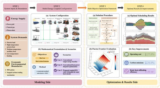
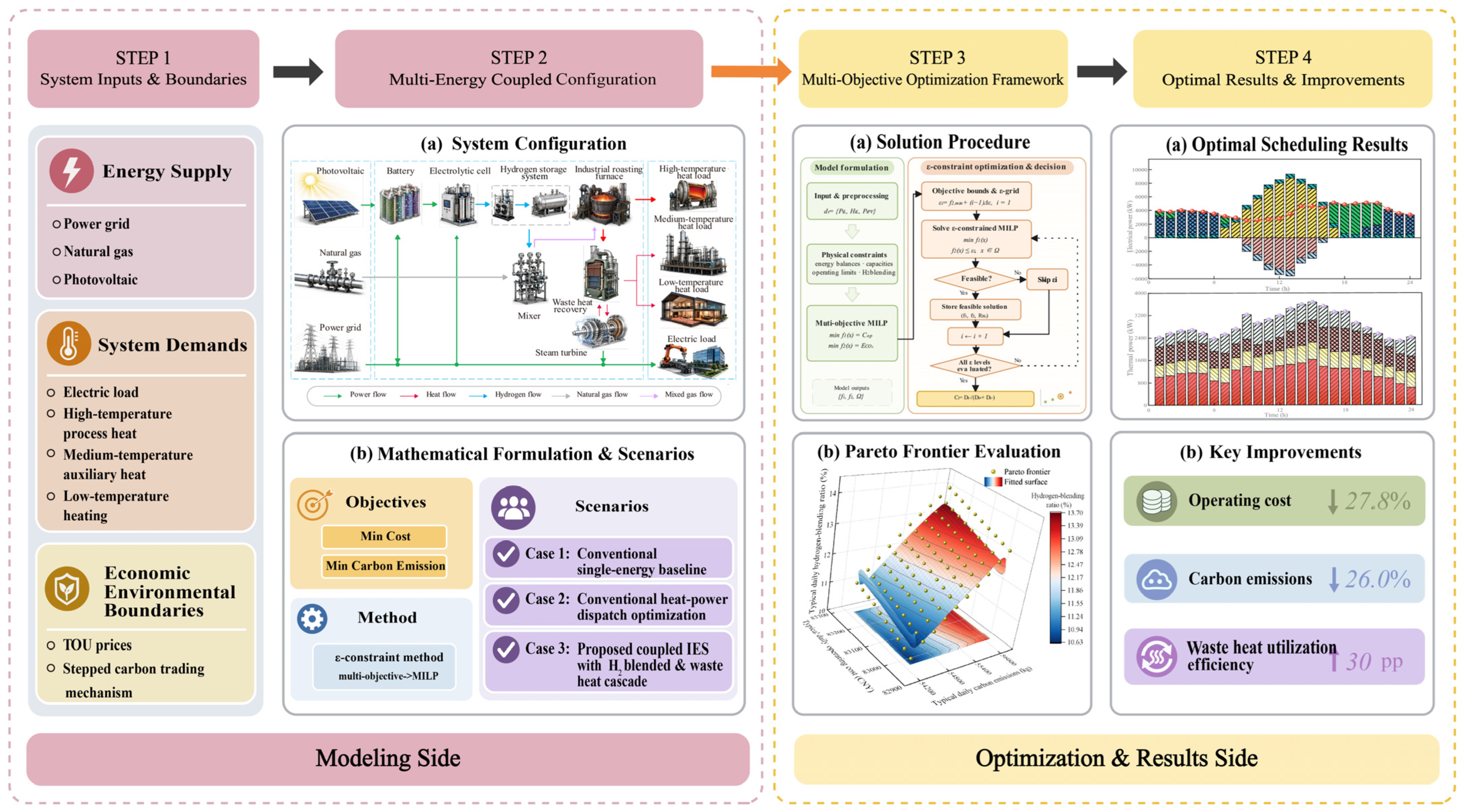
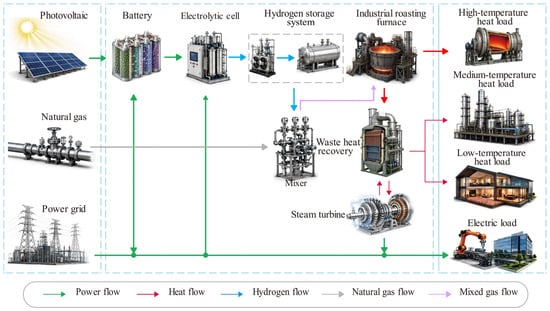
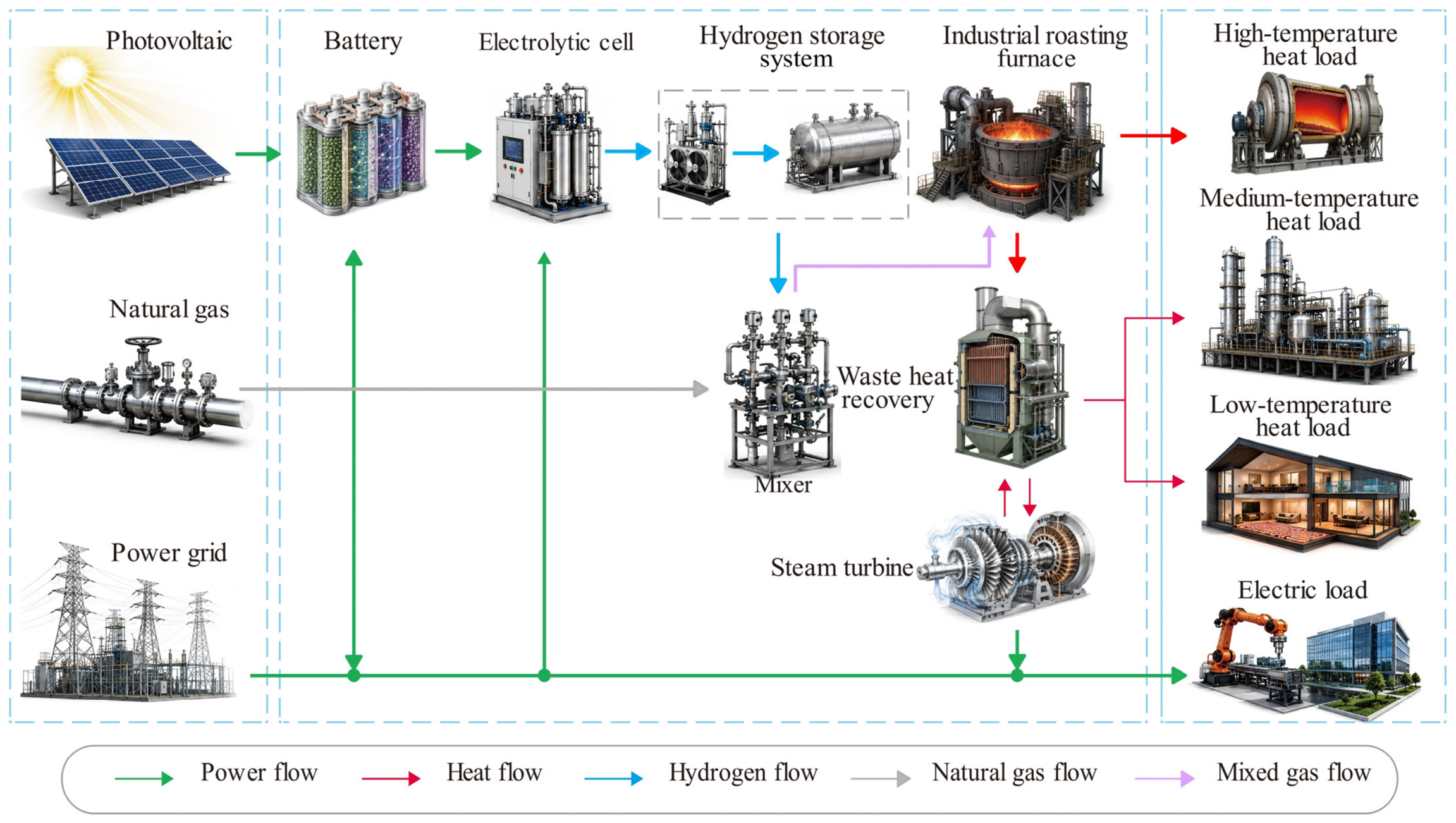
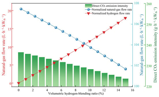
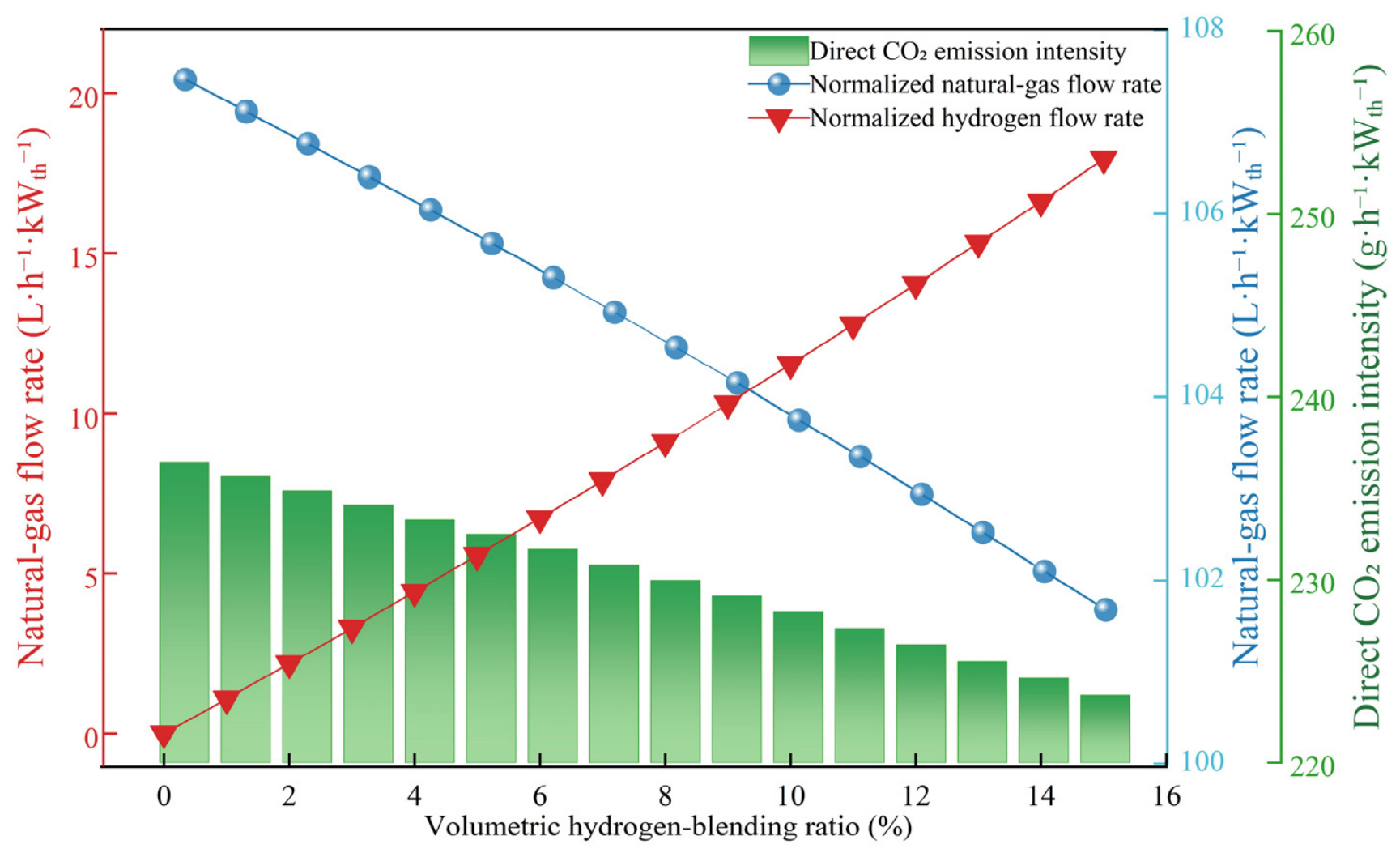
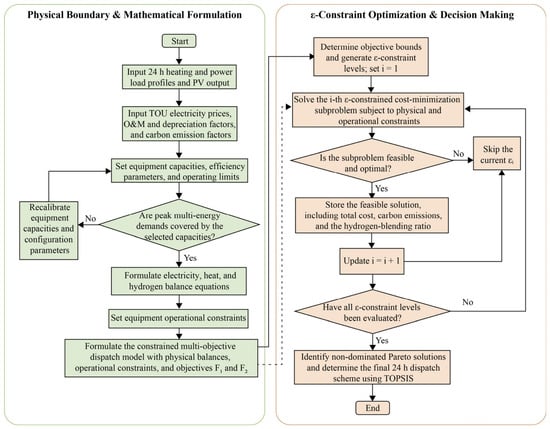
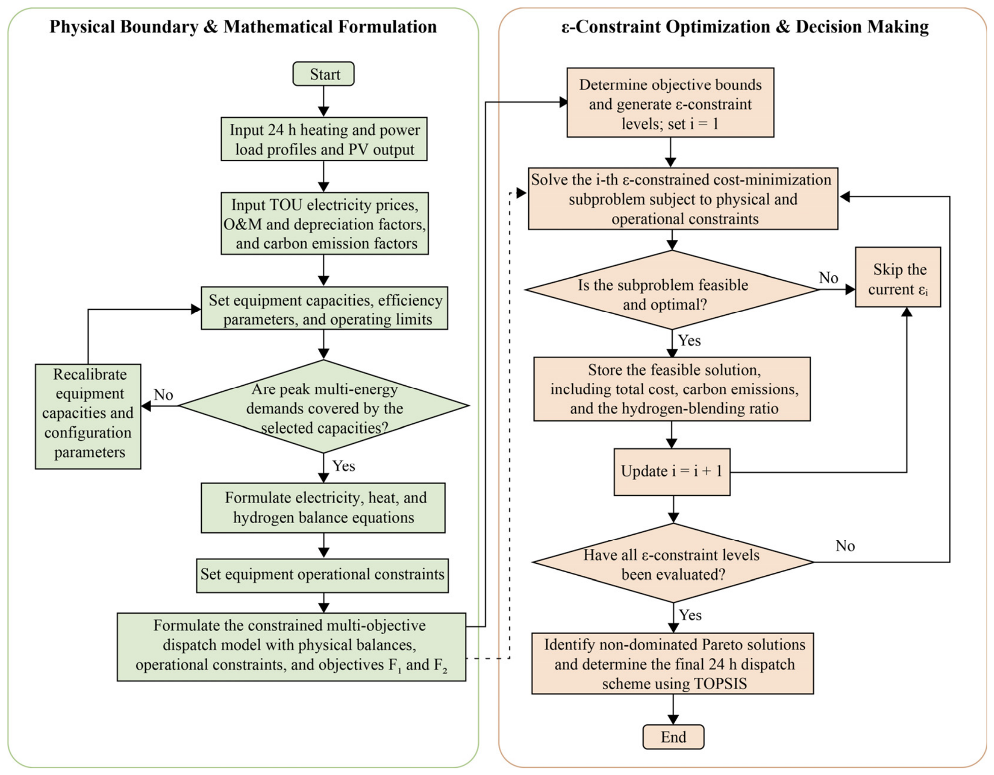
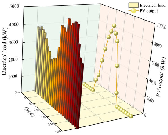
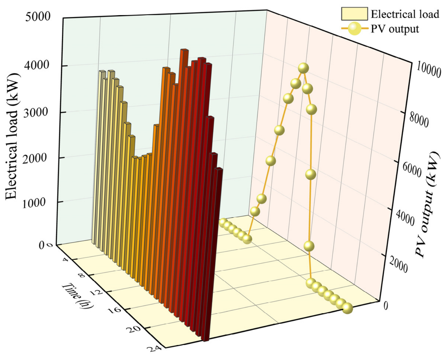
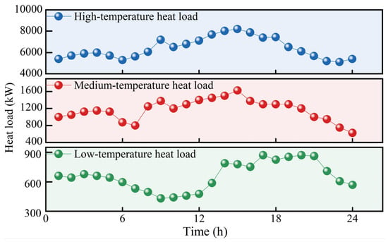
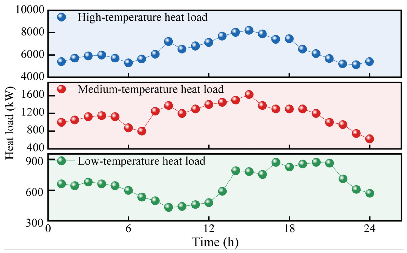
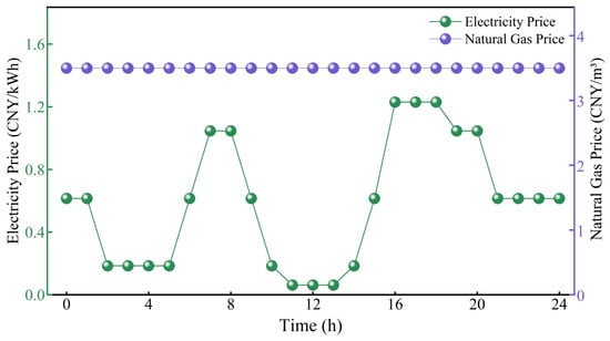
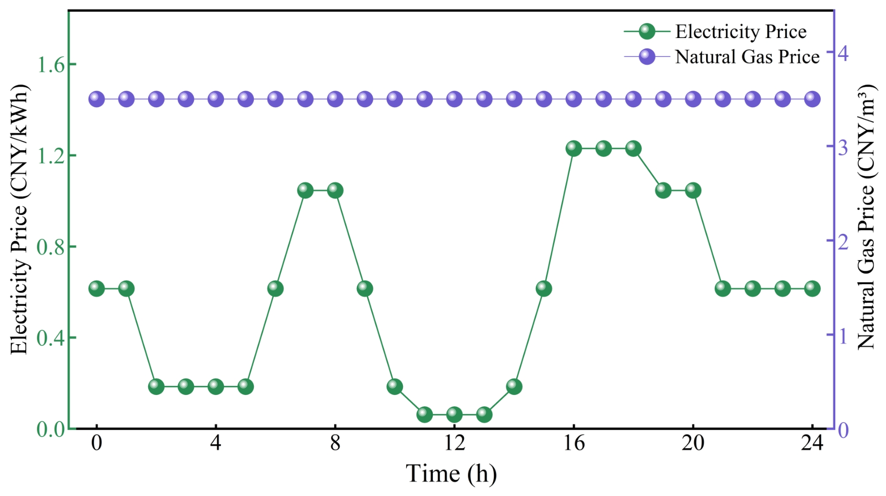
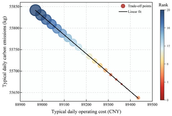
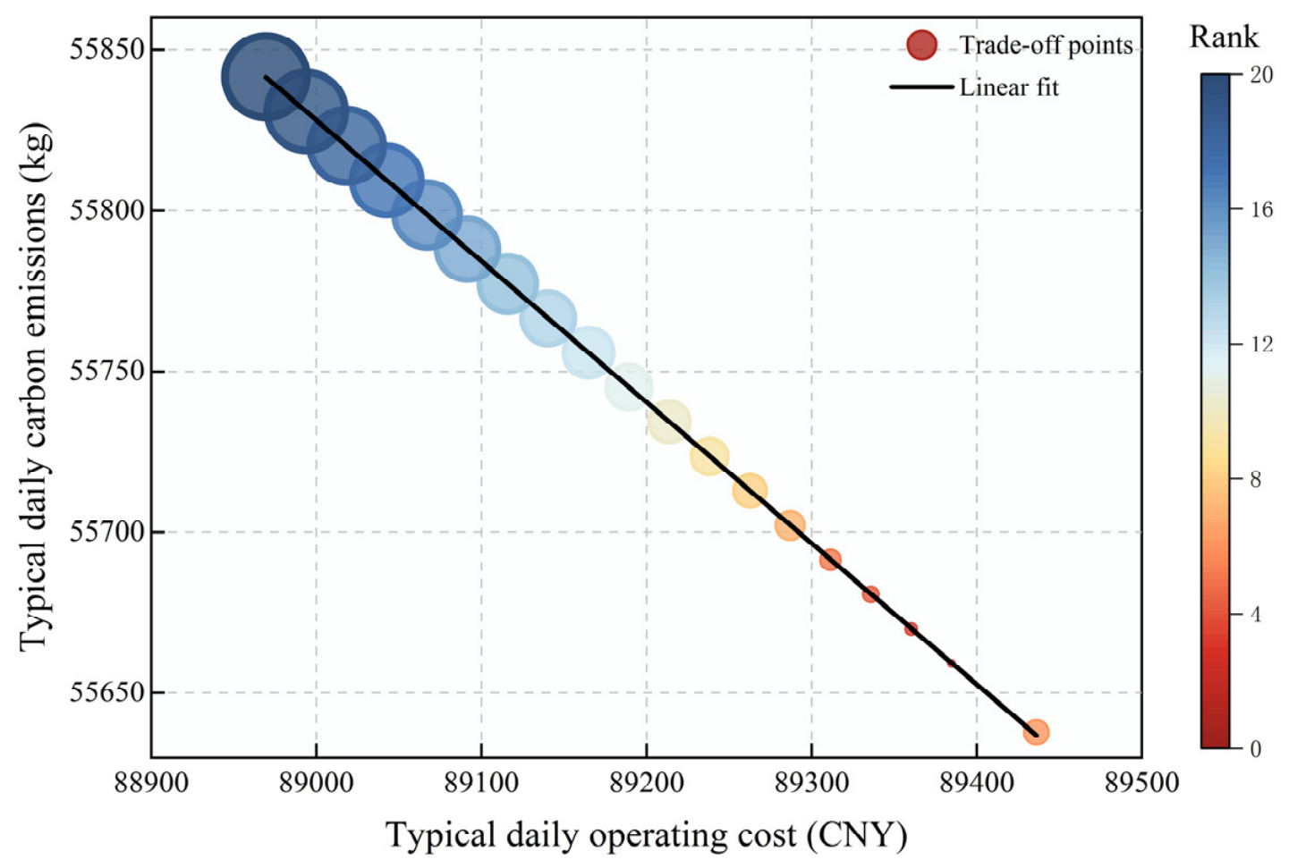
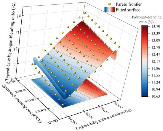
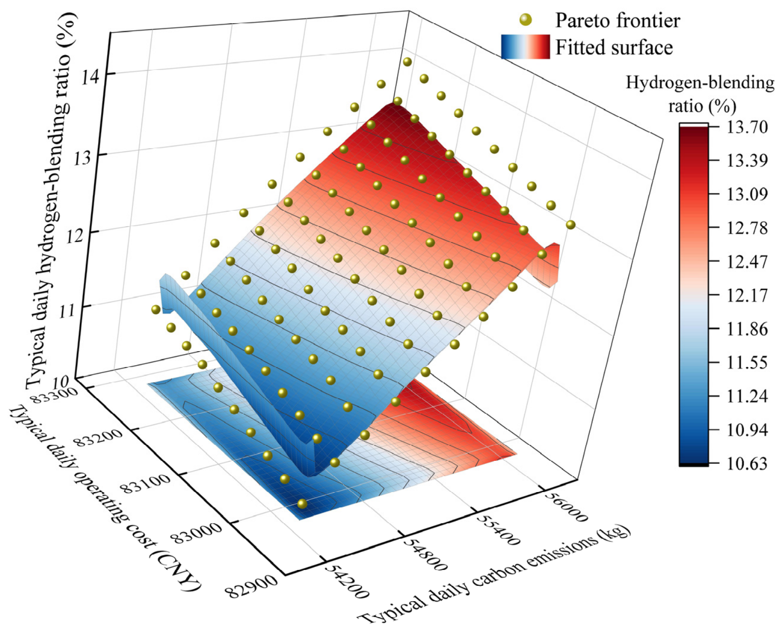
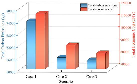
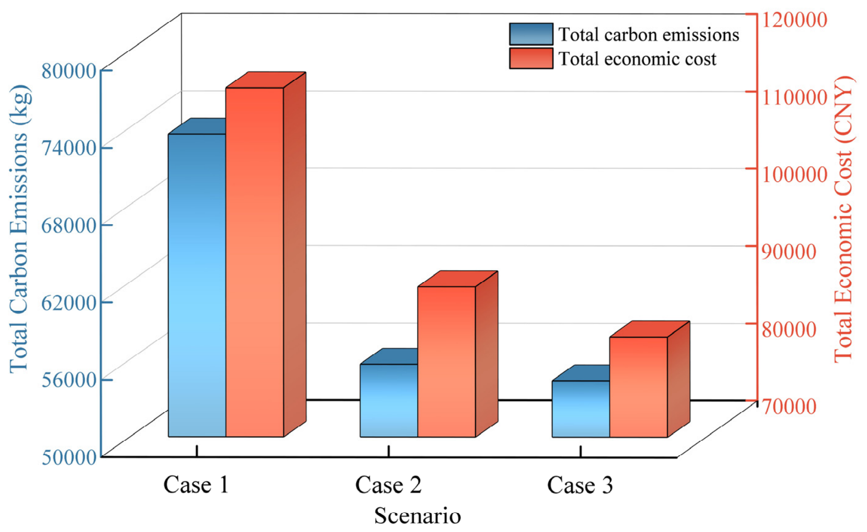
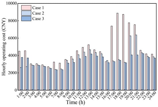
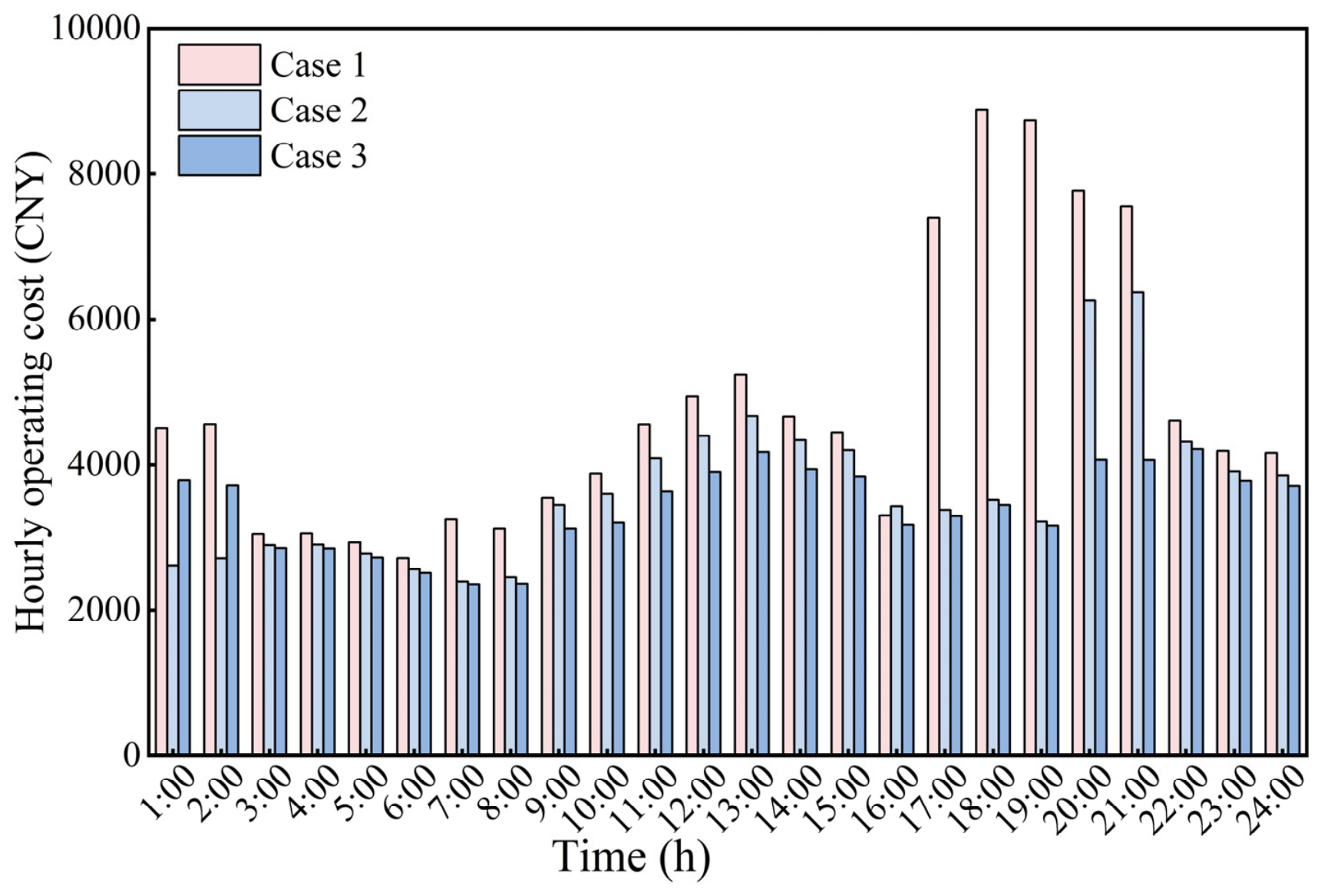
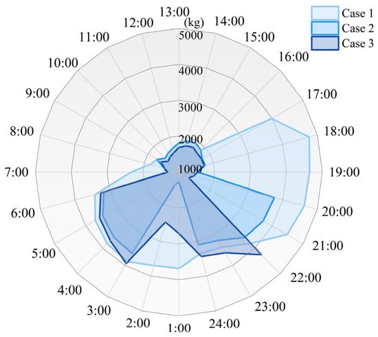
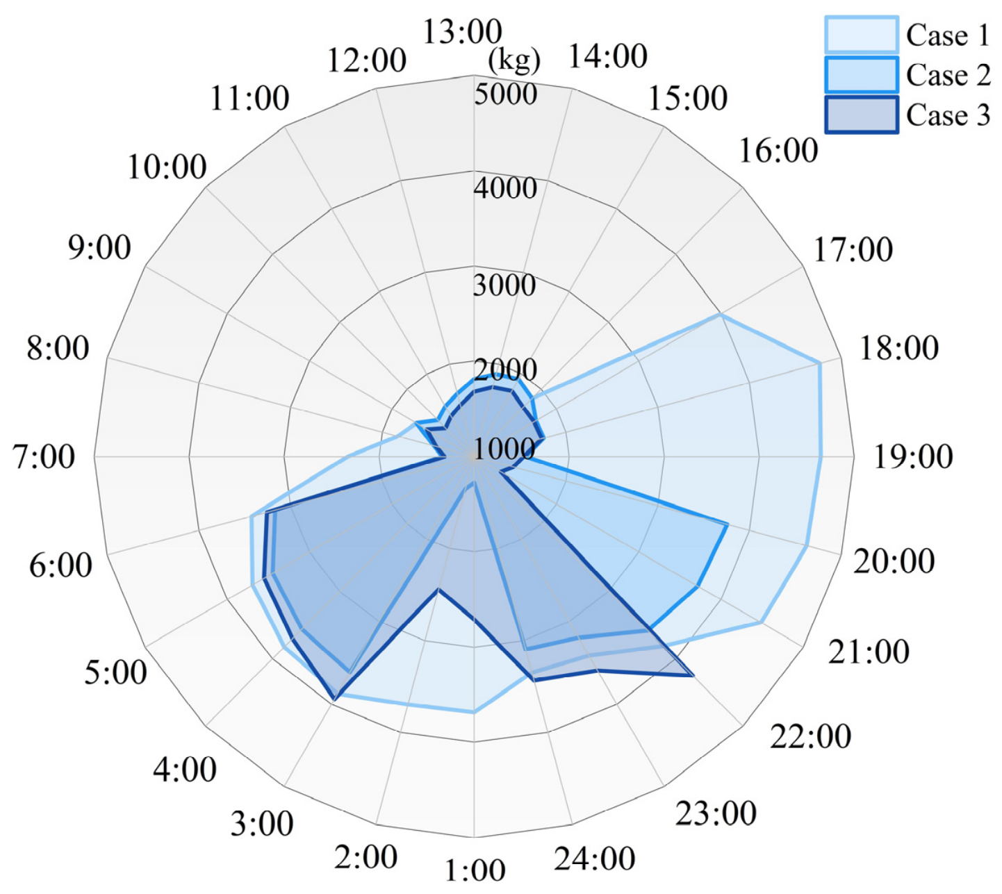
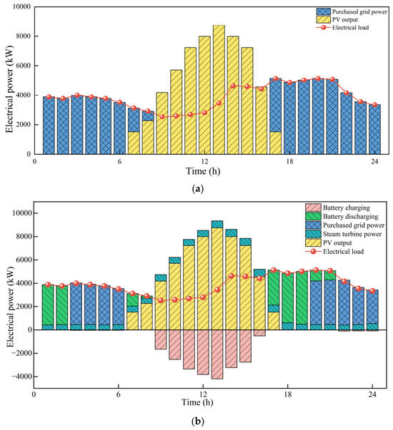
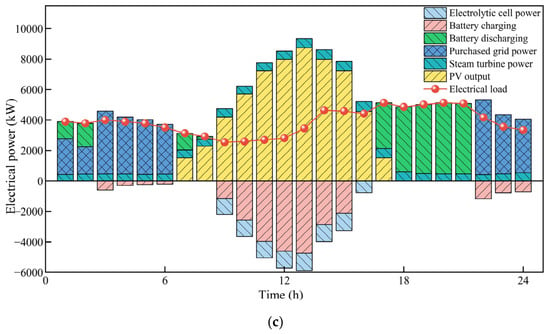
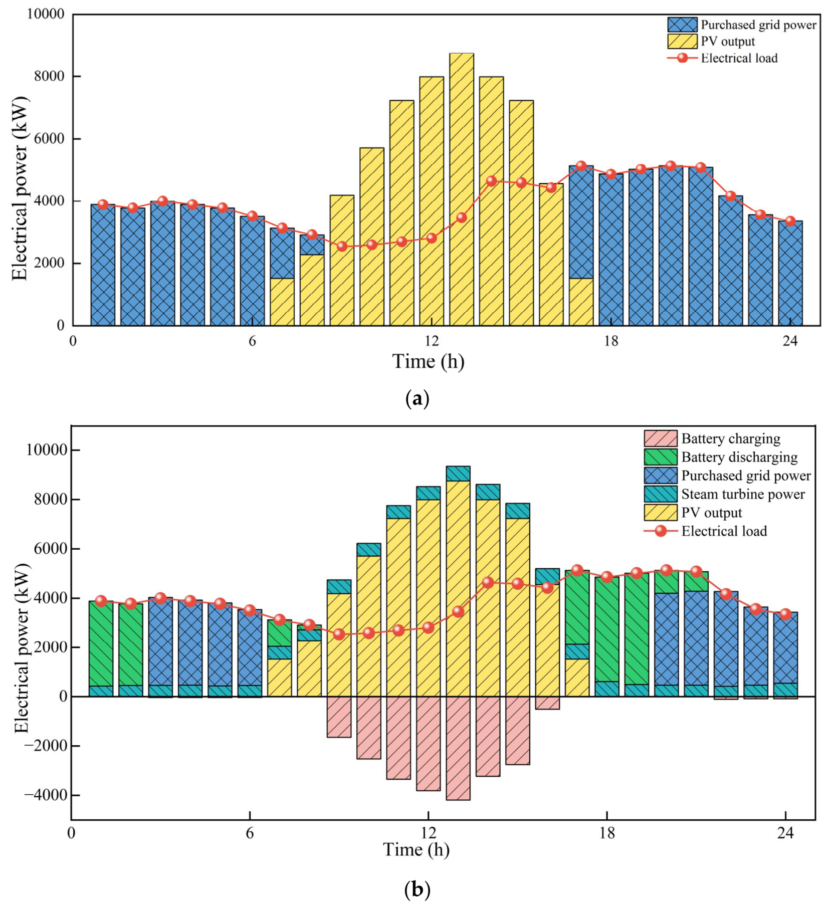
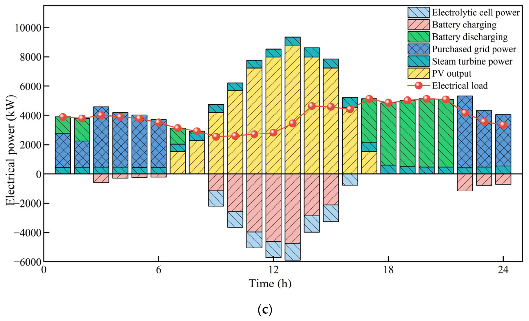
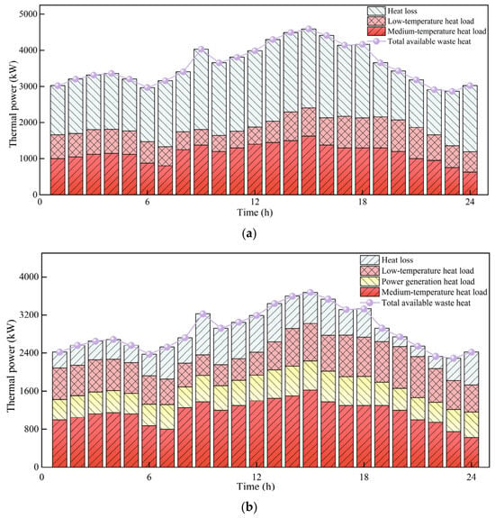
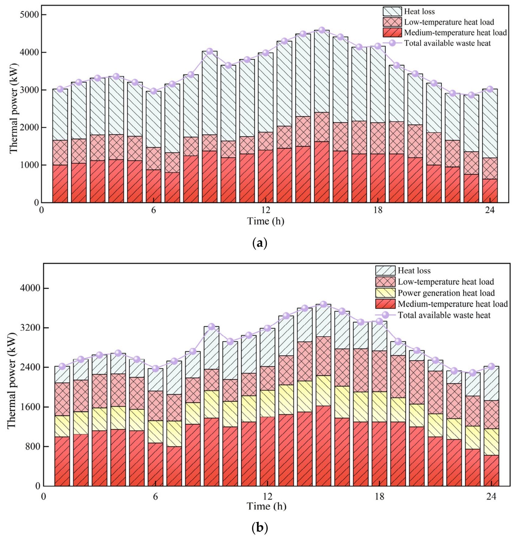
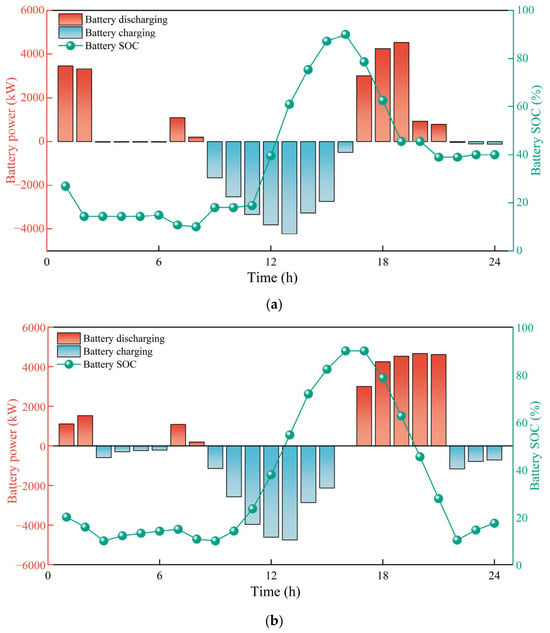
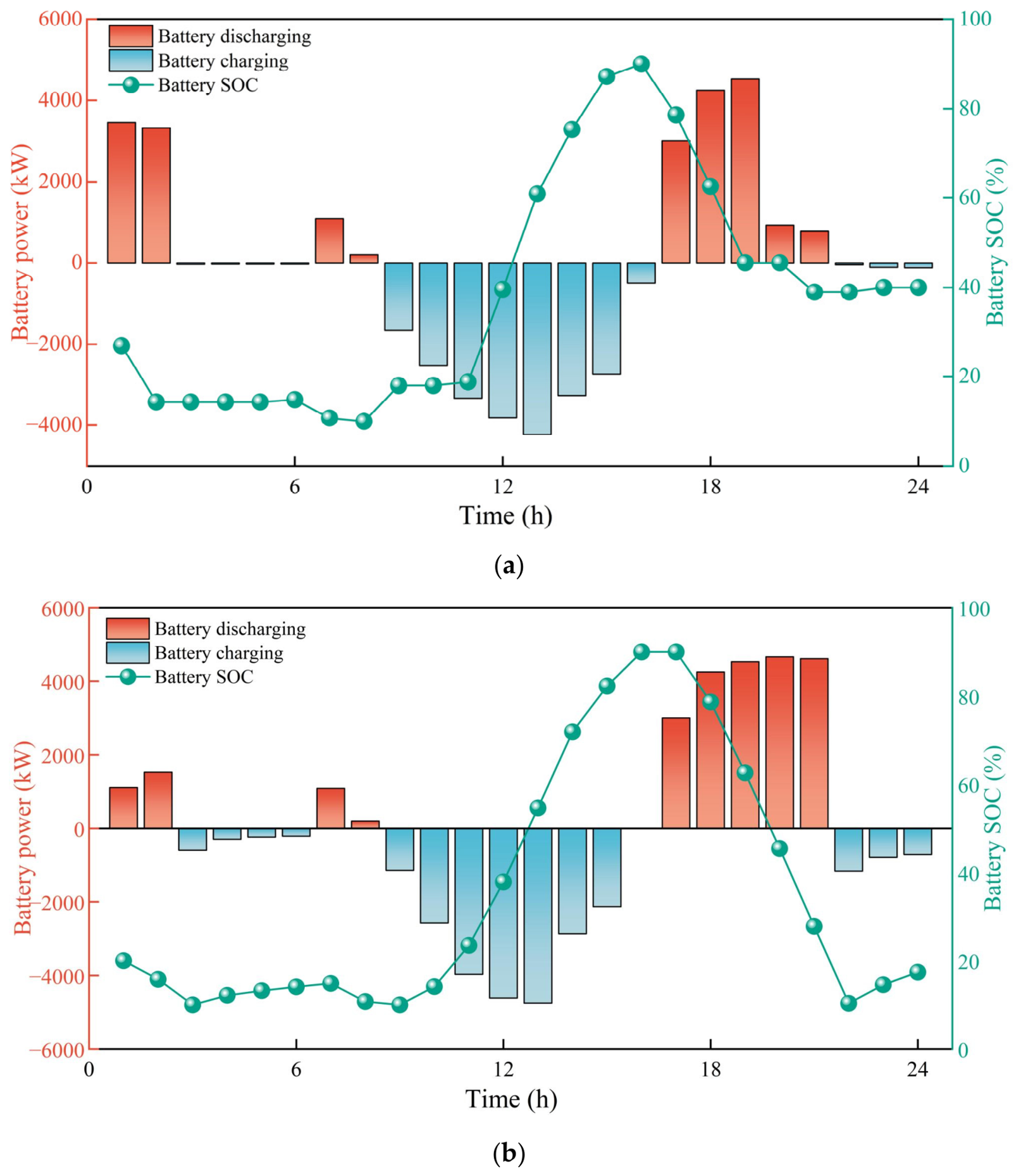
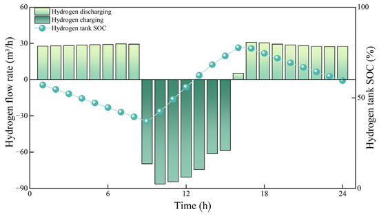
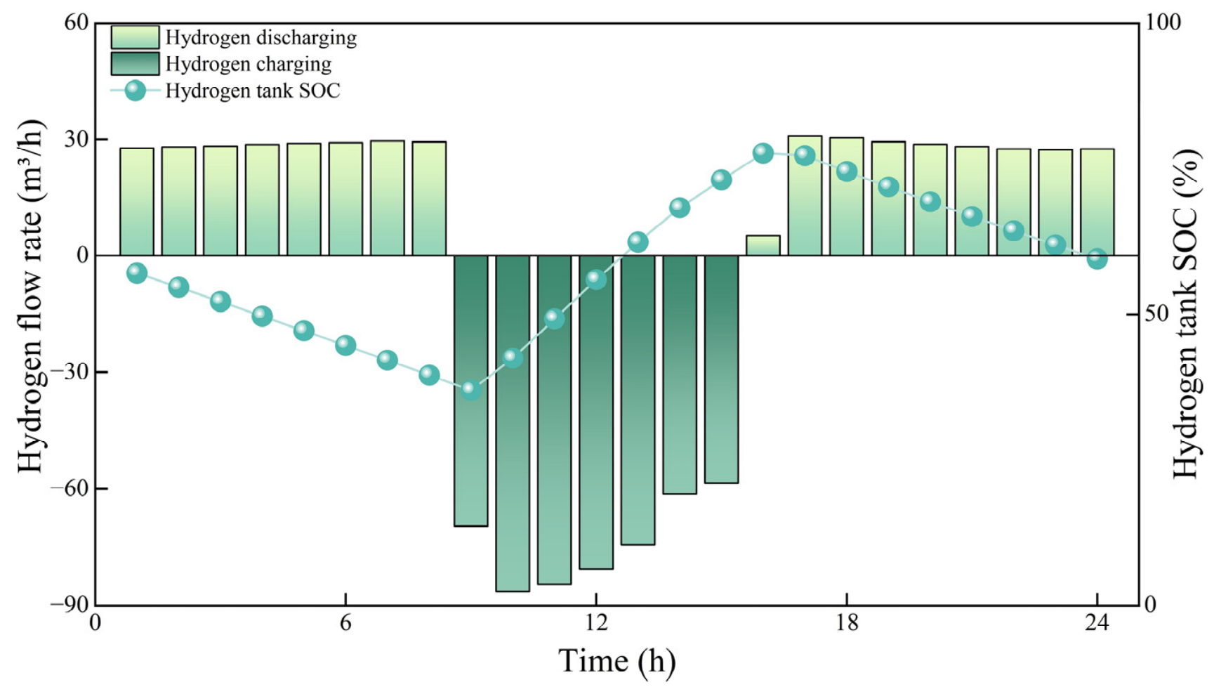

Disclaimer/Publisher’s Note: The statements, opinions and data contained in all publications are solely those of the individual author(s) and contributor(s) and not of MDPI and/or the editor(s). MDPI and/or the editor(s) disclaim responsibility for any injury to people or property resulting from any ideas, methods, instructions or products referred to in the content. |
© 2026 by the authors. Licensee MDPI, Basel, Switzerland. This article is an open access article distributed under the terms and conditions of the Creative Commons Attribution (CC BY) license.