


Abstract
With the continued advancement of low-carbon campus transformation and the increasing penetration of renewable energy, campus integrated energy systems have become key infrastructure for green campus development. However, the highly random nature of student behavior causes dynamic fluctuations in electricity, heating, and cooling loads, creating major challenges for real-time supply-demand balance and economic system scheduling. To address this problem, this paper takes student behavior uncertainty as the core disturbance factor and proposes a flexible architecture-driven autonomous adaptation and multi-energy complementary optimization strategy. A closed-loop operation paradigm of signal–response–complementarity–regulation is established, in which dynamic electricity price signals, comfort-oriented guidance, and campus functional energy-zone division are combined to form a multi-level autonomous response chain. To improve solution efficiency, the electromagnetic wave propagation algorithm is further enhanced, and a Multi-Objective Electromagnetic Wave Propagation Algorithm (MEMWPA) is developed. Wave-impedance matching and energy-flux-density feedback mechanisms are introduced to strengthen convergence performance in complex multi-objective optimization problems. Comparative case studies show that the proposed strategy can effectively smooth the net load curve, reduce the campus peak load by 26.73%, and increase the load factor by 14.533 percentage points, thereby improving both operational flexibility and energy efficiency.
1. Introduction
1.1. Research Background and Significance
Against the backdrop of accelerating low-carbon transition in university campuses and the growing penetration of distributed renewable energy, CIESs have emerged as critical infrastructure for developing green campuses, owing to their strengths in multi-energy coordination and cascade energy utilization [1,2]. The large-scale deployment of on-campus PVs and wind power supplies clean energy to the system, but also introduces inherent intermittency and output uncertainty [3]. However, campus energy loads are dominated by student activities. Behaviors including class attendance, extracurricular events, and daily living patterns are highly stochastic, which drive pronounced dynamic fluctuations in electrical, heating, and cooling demands. These fluctuations create fundamental challenges for real-time supply-demand balancing and economic system dispatch [4,5].
Existing studies have advanced campus energy scheduling from equipment-level optimization toward demand response and behavioral intervention; however, three unresolved gaps remain. First, student activities are commonly represented as static load profiles, fixed response elasticities, or exogenous stochastic disturbances [6]. Consequently, the temporal evolution of student behavior and its response to price, comfort, and operational signals are not explicitly linked to dispatch decisions. Second, behavioral intervention, multi-energy conversion, and cross-zone energy support are generally investigated as separate modules, resulting in an open-loop process in which observed load deviations cannot continuously trigger coordinated regulation actions. Third, emerging data-driven methods can improve system perception and adaptive decision-making, but their application may depend on extensive training data and does not always provide explicit guarantees for coupled electricity–heating–cooling constraints, equipment security, and user comfort.
Therefore, the scientific problem addressed in this study is how to transform uncertain student behavior from an uncontrollable external disturbance into an interpretable, constraint-aware, and optimizable resource within a campus multi-energy system. To address this problem, a closed-loop signal–response–complementarity–regulation paradigm is developed. It explicitly connects behavioral-state evolution, dynamic guidance signals, cross-zone multi-energy coordination, economic evaluation, and multi-objective optimization, thereby providing a mechanism-driven basis for autonomous campus energy regulation under behavior-induced uncertainty.
In addition, the growing demand for elderly-oriented educational and public services requires campus energy regulation to account not only for energy efficiency but also for the accessibility, acceptability, and adaptability of energy services for elderly users.
1.2. Literature Review
In the optimization of CIESs, analyzing various uncertainties is central to addressing supply-demand balance, with student behavior’s high randomness being particularly critical. Research has progressively evolved from passive response to active guidance [7,8]. For instance, a previous study by Ali et al. [9] proposes a Stackelberg game-based dynamic pricing framework with rule-based storage dispatch, reducing peak load by 18.7% and user costs by 12.3%, yet it relies on predefined response elasticities and fails to capture the time-varying nature of behavioral uncertainty specific to campus populations, limiting its adaptability to dynamic load shifts. From a behavioral perspective, studies by Chen and Lotti [10] and Zhang and Zhang [11] explore student energy-saving behaviors from experimental and game-theoretic perspectives, respectively: the former demonstrates via dormitory quasi-experiments that social-norm nudges effectively reduce accommodation energy use and foster sustained habits, while the latter identifies key behavioral drivers through evolutionary game analysis and notes that high constraint costs hinder positive transitions. Nevertheless, such micro-level behavioral insights are not operationalized into system-level dispatch logics, remaining at the stage of qualitative intervention strategies and creating a gap between behavioral research and engineering scheduling. Shifting to broader IES optimization, Chandra et al. [12] develop a three-stage energy management system with layered EV charging coordination to mitigate renewable and load uncertainties, though it targets aggregated community-level loads and lacks fine-grained autonomous response mechanisms tailored to individual behavioral patterns; complementarily, a systematic review by Carozzani and D’Alpaos [13] confirms the value of management flexibility in hybrid renewable investment appraisal under uncertainties, yet it focuses on long-term planning rather than operational strategies for daily behavioral volatility. Returning to campus-specific optimization, Ouria et al. [14] build a plus-energy microgrid integrating PV, storage, and smart parking chargers with appliance scheduling, yet prioritize physical equipment optimization and overlook short-term load fluctuations driven by dynamic student behaviors; similarly, a multi-timescale scheduling framework by Chen et al. [15] verifies the benefit of storage capacity expansion for renewable utilization, but does not incorporate signaling mechanisms to guide and shape behavioral uncertainty. In summary, while existing research explores uncertainties across multiple dimensions, further integration of fine-grained modeling and active guidance mechanisms for student behavioral uncertainty is needed to enhance overall system performance.
The optimal dispatch of IESs is crucial for enhancing energy efficiency and accommodating renewable energy [16,17]. While this field has witnessed substantial methodological progress, investigations tailored to campus-scale energy systems remain comparatively scarce. A study by Ding and Gou [18] proposes a school-centered positive energy block strategy with battery storage for solar surplus management, reducing grid dependence by 45.6% and generating annual savings of around $4.66 million, but it is confined to PV-battery power-only dispatch without considering multi-energy storage and conversion synergies. Building on this, Wang et al. [19] develop a multi-time-scale rolling optimization framework for CCHP microgrids with demand response and carbon trading, cutting operating costs by 12.4%, yet it focuses on fossil-fueled unit scheduling and lacks real-time coordination with on-site distributed renewables. Bibiloni-Mulet et al. [20] further verify the technical feasibility of 100% renewable supply via a PV-thermal hybrid zero-emission campus system with 5.3 MWh storage, but the off-grid self-sufficiency design excludes dynamic interaction with external grids or price-responsive mechanisms. From a modeling perspective, Li et al. [21] propose a linearized electricity-gas-heat coupled scheduling model that improves computational efficiency by ~40%, yet its centralized architecture fails to exploit distributed flexibility from multi-energy storage and demand-side resources. For multi-microgrid scenarios, Li et al. [22] construct a robust shared-energy-storage dispatch model with optimized benefit allocation, reducing average costs by 9.2% and raising renewable penetration by 7.8%, but it assumes fully cooperative stakeholders and disregards multi-agent gaming conflicts. To address this, Zhao et al. [23] design a bilevel Stackelberg game framework for multi-regional IES operation, increasing operator profit by 3.1% while maintaining user satisfaction; nevertheless, it treats followers as passive price-takers without accounting for competitive bidding dynamics. In summary, while existing studies have advanced in modeling and multi-energy coordination, research on campus-specific integrated dispatch remains insufficient, and further exploration is needed for dynamic, market-oriented mechanisms with multi-stakeholder competition, especially at campus and community levels.
Intelligent optimization algorithms have been widely adopted to solve complex IES scheduling problems [24,25]. Recent studies have increasingly combined intelligent optimization, forecasting, and game-theoretic mechanisms for IES scheduling. Liang et al. [26] formulated a Stackelberg-game-based optimal scheduling model for multi-community IESs considering energy interaction and carbon trading, but the study mainly emphasizes inter-community transactions rather than campus behavioral uncertainty. Li et al. [27] developed a short-term power-load forecasting framework for IESs, improving prediction accuracy under stochastic load conditions; however, the forecasting module is not embedded into a closed-loop multi-objective dispatch framework. Chen et al. [28] proposed a bi-level optimal scheduling method considering incentive-based demand response and carbon/green-certificate trading, yet user behavioral response is mainly treated as an optimization constraint rather than as an actively guided resource. Zou et al. [29] introduced an improved pelican optimization algorithm for multi-energy complementary microgrid scheduling, but its algorithmic improvement is not integrated with a campus-oriented signal–response–complementarity–regulation paradigm. In summary, while algorithm-game combinations are promising, deeper model integration and broader validation are still needed.
Beyond conventional optimization, forecasting, and game-theoretic scheduling, digital twins, RL, MASs, and XAI have become important directions in intelligent energy management. Digital-twin-enabled building energy management systems establish continuously updated virtual representations of physical assets and operating states, thereby supporting information fusion, performance evaluation, and predictive control [30]. Their main advantage lies in real-time synchronization between physical systems and virtual models. However, their practical performance depends strongly on sensing infrastructure, model calibration, and bidirectional data exchange, and a digital twin alone does not determine how behavior-induced load deviations should be converted into coordinated multi-energy regulation actions.
RL obtains sequential control policies through interaction with the operating environment and has been applied to the joint prediction and scheduling of IESs [31]. It provides adaptability under uncertain and time-varying conditions, but policy training, constraint satisfaction, operational safety, and transferability remain important issues in campus systems involving strongly coupled electricity, heating, cooling, storage, and comfort requirements. MASs, particularly multi-agent deep RL, decompose complex energy systems into interacting agents and support distributed coordination among devices, subsystems, and market participants [32]. Nevertheless, existing agents are generally defined according to equipment, microgrids, or economic entities, whereas student behavioral states, guidance acceptance, and mutual support among campus functional zones have rarely been incorporated into a unified response chain. XAI can improve the transparency and credibility of forecasting and automated energy-management decisions by identifying the factors that influence model outputs [33]. However, explaining the output of a data-driven model is different from constructing an inherently interpretable regulation mechanism with explicit physical constraints and traceable signal-to-action relationships.
These developments demonstrate the value of digital perception, adaptive learning, distributed intelligence, and decision transparency. Nevertheless, a research gap remains in integrating behavior-oriented response, physically constrained multi-energy coordination, and traceable closed-loop regulation within a unified campus operational framework. The present study addresses this gap through a mechanism-driven optimization architecture rather than directly replacing the dispatch process with a black-box learning policy.
Table 1 compares the characteristics of existing research.
Table 1.
Comparison of representative related studies.
1.3. Innovation and Contributions
Based on the above research gaps, the scientific contribution of this study is a mechanism-driven, closed-loop formulation for behavior-aware campus multi-energy regulation. Instead of treating student behavior only as an exogenous random load or relying entirely on a data-driven policy learner, the proposed framework represents student behavior as a state-dependent response resource that can be influenced by price and comfort signals and coordinated with physical energy conversion and cross-zone energy support. The resulting signal–response–complementarity–regulation chain establishes an explicit and traceable mapping from behavioral-disturbance perception to feasible dispatch actions, while economic cost, carbon emissions, incentive benefits, storage degradation, and user comfort are retained as independent optimization objectives.
On this basis, the methodological addition is reflected in the integration of behavioral-state transition, autonomous response, multi-energy complementarity, and Pareto-based decision-making within the same closed-loop framework. The computational addition is the development of MEMWPA, in which wave-impedance matching and energy-flux-density feedback are introduced to adaptively coordinate global exploration and local exploitation. Therefore, the contribution of this study is both conceptual—redefining student behavioral uncertainty as an endogenous and optimizable flexibility resource—and methodological—providing a physically constrained and interpretable solution for closed-loop campus multi-energy operation. The specific contributions are fourfold.
- A collaborative operation mechanism integrating flexible architecture and autonomous response is proposed. By designing dynamic electricity pricing and comfort signals as guiding instruments, and by dividing the campus into distinct functional zones, a multi-level autonomous response chain is established. This enables the system to automatically adapt to real-time load signals, thereby enhancing its inherent resilience against sudden load fluctuations and achieving a shift from passive accommodation to active guidance.
- A closed-loop optimization framework that integrates signal response with multi-energy complementarity is constructed. This framework organically combines flexible guidance signals, user-side autonomous response behaviors, and the conversion rules among electricity, heat, and cooling energies, together with cross-zone mutual support strategies, to form a complete closed-loop regulation chain. This design effectively smooths random load fluctuations and improves both the on-site consumption rate of renewable energy and the overall energy utilization efficiency.
- An autonomous decision-making model embedded with economic evaluation is incorporated. Each response action is associated with a simplified cost-benefit function, which is rapidly assessed prior to execution. Actions are then prioritized and executed according to their economic rank. This mechanism ensures that the system enhances operational flexibility and security without compromising its economic objectives, thereby achieving a unified balance between safety and cost-effectiveness.
- An improved MEMWPA has been developed, providing an efficient solution tool for complex models. In view of the high-dimensional and nonlinear characteristics of the model, this paper improves the standard EMWPA algorithm by adaptively adjusting the search parameters based on the “wave impedance matching” concept and dynamically balancing exploration and exploitation through “energy flux density feedback”. The improved MEMWPA algorithm demonstrates advantages in terms of convergence accuracy, distribution uniformity, and stability when solving the model in this paper and standard test problems.
In summary, the contribution of this work is not a simple superposition of individual technical elements, but rather the deep synergy among the above four mechanisms, forming a complete closed-loop system encompassing signal triggering, autonomous decision-making, multi-energy coordination, economic validation, and feedback optimization. This framework brings student behavioral uncertainty under the system’s controllable scope, providing both theoretical support and engineering reference for the intelligent dispatch of CIESs under highly uncertain environments.
2. Modeling and Optimization Framework of CIES
To facilitate readability and ensure the mathematical rigor of the proposed models in terms of physical dimensions, Table 2 summarizes the standard units adopted for all key physical variables involved in the formulas throughout this paper. Unless otherwise explicitly stated in the specific context of a particular equation, all power variables (including electricity, heating, and cooling) are uniformly expressed in kW, all energy storage capacities in kWh, all energy prices in $/kWh, and all temperature variables in °C. It should be noted that efficiency coefficients, coefficients of performance (COP), response coefficients, probability parameters, and binary logic indicators are dimensionless. This unified convention is applied consistently across the subsequent modeling and case study sections to avoid dimensional ambiguity.
Table 2.
Notation and units for the main variables used in the proposed model.
2.1. The Framework of CIES
The CIES achieves optimal energy efficiency, minimal operating costs, and lowest carbon emissions by coordinating the synergistic interaction of generation, grid, load, and storage. This ensures energy demand is met for core functional areas such as dormitories, teaching buildings, and activity centers. The core operational mechanism of CIES is based on multi-energy complementarity, flexible load control, and carbon-energy co-optimization. It involves the coordinated operation of the CES, the CEDC, and three typical energy consumption zones: the dormitory area, the teaching building area, and the activity center area. The dormitory area focuses on residential energy use and demand response. It primarily integrates rooftop PVs and HPs for domestic hot water supply, equipped with smart meters and outlets for refined electricity management. Its energy storage systems can participate in nighttime grid regulation. The Academic Building Zone prioritizes stable teaching environments and energy efficiency. It typically deploys building-integrated PVs, high-efficiency central AC, and fresh air systems. Leveraging class schedules, the intelligent building system pre-regulates classroom lighting and AC through time-based, zone-specific controls. As the area with the most fluctuating energy loads on campus, the activity center emphasizes flexibility and backup capacity. Beyond distributed PV, it can be equipped with rapid-response energy storage devices and integrated into the campus energy management system. During large events, it can draw on surplus power or stored energy from other zones. These three areas are interconnected through a campus-wide integrated energy management system, enabling energy complementarity. Customized deployment of PV systems, HPs, and energy storage devices is tailored to each zone’s specific energy characteristics—such as residential rhythms in dormitories, teaching schedule requirements, and fluctuating activity loads—to achieve precise energy provisioning. Simultaneously, the campus electricity and thermal networks interconnect energy production, storage, and consumption nodes across all zones. The specific framework is illustrated in Figure 1.
Figure 1.
Framework of CIES.
2.2. The CIES Model
Energy storage equipment serves as the primary vehicle for campus electricity storage. Its core function lies in smoothing out the intermittent fluctuations of PV and wind power generation, achieving peak shaving and valley filling to reduce electricity costs, while providing emergency power supply to safeguard critical loads during grid failures. HS equipment serves as a buffer between the heat source and load sides within campus heating systems. It resolves the temporal mismatch between heat generation capacity and thermal demand, acting as a critical enabler for efficient and flexible heating system operation. The specific model is as follows:
where Et,ES represents the electricity storage level of the ES device at the current time t; Ht,HS denotes the HS level of the HS device at the current time t; ωe,ch is the charging efficiency of the ES device; ωt,di is the discharging efficiency of the ES device; Pt,ch is the charging power; Pt,di is the discharging power; Ht,ch is the heat charging power; ζe represents the self-discharge rate of the ES device in idle state; ωh,ch is the conversion efficiency of the HS device during the heat storage process; ζh denotes the thermal loss coefficient of the HS device when inactive.
The GT achieves CCHP through the efficient utilization of natural gas, making it suitable for campus cogeneration systems. The specific mathematical model is shown in the formula below:
where Pt,gt represents the electrical power generated by the GT; Ht,gt denotes the thermal energy output by the GT during time period t; is the power generation conversion efficiency; is the energy loss coefficient during GT operation; hHV is the lower heating value of natural gas; Vt,gt is the volume of natural gas consumed.
The core function of the WHB is to recover the waste heat from high-temperature flue gases discharged by power equipment such as GTs and gas internal combustion engines. The GB is a fundamental heat source device that ensures the campus’s thermal energy supply. The specific mathematical model is shown in the following formula:
where Ht,gb represents the thermal power output of the GB during time period t; Ht,hr is the effective thermal power output of the WHB during time period t; Vgb is the volume of natural gas consumed by the GB in that period; is the heating efficiency of the WHB, which characterizes its ability to recover high-temperature waste heat and convert it into usable thermal energy; Hi,hr is the total amount of high-temperature waste heat available for recovery, typically sourced from exhaust heat of upstream equipment such as GTs; and is the heat production efficiency coefficient of the GB, reflecting its conversion efficiency in transforming the chemical energy of natural gas into thermal energy.
PV Power Generation Equipment is a core component in achieving clean energy substitution and reducing carbon emissions. Wind Power Generation Equipment serves as an important supplementary form for utilizing wind energy resources within the CIES. The specific mathematical model is as follows:
where Pt,pv represents the output power of the PV system during time period t; Pt,wt denotes the output power of the wind power generation equipment during time period t; Pn,pv is the rated output power of the PV module; Lt is the solar irradiance intensity during the current period; tn is the reference temperature under standard test conditions; Lst is the solar irradiance intensity under standard test conditions; gpv is the temperature correction factor for PV power; wi is the minimum wind speed required to start the WT; wn is the wind speed at which the rated output power is reached; wo is the cut-out wind speed at which the turbine stops operating for safety reasons; and Pn,wt represents the rated power of the WT.
The preceding subsections have modeled the supply-side and storage-side equipment. However, lighting, as one of the most flexible end-use loads on campus and a key adjustable resource under student behavioral uncertainty, has not yet been explicitly formulated. The complete lighting load model, including the physical relationship among lighting power, dimming commands, daylight contribution, and visual comfort constraints, is developed as follows.
- (1)
- Relationship between lighting power and illuminance
- (2)
- The strict definition of dimming commands and “brightness percentage”
- (3)
- Daylight contribution model
- (4)
- Hard constraint of visual comfort
- (5)
- Thermal comfort representation
Although a detailed lighting model is explicitly introduced to characterize visual comfort, thermal comfort is also an essential component of user satisfaction in CIESs. In this study, instead of introducing a highly complex physiological comfort model (e.g., PMV-PPD), a simplified temperature-based thermal comfort representation is adopted.
The main reason is that the proposed model focuses on campus-scale multi-energy scheduling rather than individual-level building environment simulation. Detailed thermal comfort models require additional parameters, including metabolic rate, clothing insulation, air velocity, relative humidity, and mean radiant temperature, which are difficult to obtain dynamically during campus operation. Therefore, indoor temperature is selected as the dominant controllable variable because it directly interacts with heating and cooling energy consumption and can be adjusted through HVAC systems.
The thermal comfort deviation is quantified based on the deviation between the indoor temperature and the preferred comfort range:
where represents the indoor temperature at time t, and represents the preferred comfort temperature. The corresponding thermal comfort penalty is incorporated into the multi-objective optimization framework together with visual comfort.
However, relying solely on a penalty term may not guarantee that the temperature stays within an acceptable comfort band under all operating conditions, especially when extreme disturbances occur or when the penalty weight is insufficient. To address this, a hard constraint is further imposed to strictly bound the indoor temperature:
where and are the lower and upper acceptable temperature limits. This constraint ensures that any optimized solution respects the basic thermal comfort requirement, complementing the penalty-based deviation term and enhancing the reliability of the proposed strategy.
This simplified approach provides a balance between physical interpretability and computational efficiency, while maintaining consistency with the system-level optimization objective of the pre-defined CIES framework.
In the CIES, to ensure the safe, stable, and economical operation of multiple energy-consuming areas such as dormitories, teaching buildings, and activity centers, comprehensive power balance equations and various operational constraints must be established. The CIES aims to minimize the total operating cost while balancing the economic interests of all participating entities, the CEDC, and three typical energy-consuming areas: the dormitory zone, teaching building zone, and activity center zone.
The CIES takes the minimization of total operating cost as its optimization objective, comprehensively considering energy procurement costs, equipment O&M expenses, and carbon emission costs, while also accounting for the benefits from flexible load response and energy sales revenue. The system covers three typical energy-consuming areas—the dormitory zone, teaching building zone, and activity center zone—and is coordinated and optimized by the CEDC. The formula is as follows:
where CostCIES represents the total operating cost of the CIES; Coste denotes the energy procurement cost, covering expenses for purchasing electricity from the external grid, natural gas, and other energy sources; Costop refers to the equipment O&M cost, encompassing the operational and maintenance expenditures for devices such as GTs, boilers, and energy storage systems; Costca stands for the carbon emission cost, calculated based on the campus carbon emissions and carbon trading prices; Rf indicates the revenue from flexible load response, obtained through incentive compensations from participating in demand response programs; while Rse represents the revenue from energy sales, generated by selling surplus electricity or thermal energy to the external grid or other users.
The power balance constraint ensures the real-time supply and demand balance of electric energy in the campus. The total demand on the power generation side (base load, electric refrigerator, energy storage charging) must be equal to the total supply on the power generation side (PV, wind power, GT, external power purchase, energy storage discharge) minus the electricity sold. Thermal power balance constraints ensure real-time matching of campus thermal energy supply and demand. The cold power balance constraint maintains the balance between supply and demand of campus cold energy. The cooling load demand is shared by electric refrigerators and absorption refrigerators. The formula is as follows:
where Pt,load represents the total electrical load demand of the campus during time period t; Ht,load denotes the total thermal load demand of the campus during time period t; Ht,HS,di is the heat discharge power of the HS device during time period t.
As a centralized energy production and conversion center in the campus, the goal of the CES is to maximize operating income or minimize operating costs under the premise of campus energy demand. Usually, the formula is used to consider energy sales revenue, fuel costs, equipment O&M costs, carbon emission costs, etc. The formula is as follows:
where RCES represents the total net revenue of the CES; and denote the selling prices of electricity and heat during time period t, respectively; Pt,se and Ht,se represent the power of electricity and heat sold by the CES during time period t; Costt,fu is the fuel cost during time period.
For the internal energy balance constraints of the CES, the formula is as follows:
where Pt,self,CES and Ht,self,CES represent the self-consumption power of electricity and heat loads of the CES during time period t.
As the centralized dispatching and coordination center of the campus energy system, the campus energy dispatching center is responsible for optimizing the energy flow of the entire campus. The goal is usually to minimize the total operating cost of the campus or maximize social benefits, while ensuring the reliability and low-carbon nature of energy supply. The formula is as follows:
where CostEDC represents the total operating cost of the campus energy system; Costt,pu is the cost of purchasing energy (electricity, gas) from external sources during period t; Costt,op is the O&M cost for all equipment (including the CES and regional equipment) during period t; Rdr,t is the demand response revenue during period t.
To avoid the subjective bias caused by directly assigning fixed weights to conflicting objectives, the proposed optimization problem is first formulated as a genuine multi-objective optimization problem. Specifically, economic cost, carbon emission, incentive benefit, storage degradation, and user comfort are treated as independent objectives. After obtaining the Pareto frontier, a decision-making procedure is introduced to determine the final dispatch scheme.
For the overall energy balance constraint of the campus, the formula is as follows:
where r belongs to the dormitory zone, the teaching building zone, or the activity center zone; Pt,CES,su is the electrical power delivered by the CES to the campus; Pt,loss,gr is the power loss in the campus grid; Ht,hp,r is the thermal power supplied by the HP in region r; Ht,sol,r is the solar thermal energy collected in region r.
The power generation and heat generation of GTs must be within the allowable range of the equipment, and the power changes in adjacent periods are limited by the climbing rate. Its device constraints are as follows:
where Pmin,gt and Pmax,gt represent the lower and upper limits of power generation for the GT; Hmin,gt and Hmax,gt denote the lower and upper limits of thermal power output for the GT, respectively; ∆Pmin,gt and ∆Pmax,gt represent the downward and upward ramping rate limits for power generation.
During the scheduling horizon, the energy storage devices must not only satisfy the long-term state-of-charge dynamics but also strictly comply with their instantaneous physical boundary limits regarding capacity and charging/discharging rates. Furthermore, simultaneous charging and discharging states must be mathematically suppressed to avoid physical conflicts:
where Emin,ES and Emax,ES represent the minimum and maximum allowable electrical capacities of the ES system, respectively; Pmax,ch and Pmax,di denote the maximum charging and discharging power limits of the ES, respectively; ut,ch and ut,di are binary decision variables indicating the charging and discharging states of the ES at time interval t (where 1 represents active and 0 represents suppressed); Hmin,HS and Hmax,HS signify the lower and upper bounds of the HS capacity, respectively; Hmax,ch and Hmax,di are the maximum charging and discharging heat rates of the HS, respectively; and vt,ch and vt,di are binary variables reflecting the charging and discharging states of the HS at time interval t, enforcing mutual exclusivity.
When the campus microgrid exchanges electricity with the external utility grid, the power trading is strictly constrained by the substation transformer capacity and the thermal stability limits of the transmission lines. Concurrent bidirectional power flows are mathematically suppressed to prevent logical redundancy:
where Pgrid,max represents the maximum allowable safe power transmission capacity of the tie-line connecting the campus microgrid and the EM; Pt,gr,buy and Pt,gr,se signify the grid-purchased and grid-sold power at time interval t, respectively; and zt,buy and zt,se denote binary factors indicating the purchasing and selling states at time interval t, respectively, ensuring a unique power flow direction at any given instant. More constraints related to other equipment can be found in ref. [34].
To provide a rigorous mathematical foundation for the proposed strategy, the control actions are formulated as a multi-objective optimization problem rather than heuristic rules.
The multi-objective optimization problem is formulated as follows:
where Cen denotes the electricity purchasing cost under time-varying tariffs; Ccar represents carbon emission costs under carbon pricing mechanisms; Rinc is the incentive revenue obtained from demand response participation; Cdeg accounts for energy storage degradation costs; Dcom quantifies the comfort deviation penalty.
The energy cost is calculated as:
where πt is the time-of-use electricity pricing; πCO2 is the carbon price and ηgrid is the emission factor; ρt denotes the incentive price for demand response; cdeg represents the degradation cost coefficient; Tt and It denote the indoor temperature and lighting level at time t, respectively; Jage denotes the satisfaction index of age-friendly services. Instead of being an independent evaluation metric, Jage is integrated into the optimization objective to guide the coordinated adjustment of indoor temperature, lighting intensity, and energy management strategies.
The objective functions in Equation (21) have different physical units and magnitudes. To prevent dominance of objectives with larger numerical ranges, a normalization procedure is applied before evaluating the Pareto front. For each objective f, the normalized value is computed as:
where fmin and fmax are the ideal and nadir values obtained from the current population, and ϵ is a small positive constant to avoid division by zero. This min-max scaling maps all objectives onto [0, 1], ensuring equal contribution to the crowding distance and selection pressure.
The conflict among objectives is inherent due to competing priorities: reducing energy cost tends to increase comfort deviation, while lowering carbon emissions may require higher renewable investment and storage cycling. This multi-objective conflict is handled by the Pareto dominance principle, where a solution x dominates another solution y if f(x) ≤ f(y) for all objectives and strictly for at least one. No single optimal solution exists; instead, a set of non-dominated solutions is generated by the MEMWPA algorithm.
To select a single dispatch scheme from the Pareto front for practical implementation, a decision-making strategy combining crowding distance and reference-point proximity is adopted. The crowding distance CD measures the diversity of solutions; solutions with larger CD are preferred to maintain spread. Meanwhile, a reference point fref is defined based on the decision-maker’s preference (e.g., equal emphasis on cost and comfort). The final solution is chosen as:
which balances proximity to the desired reference point and diversity. This procedure ensures that the final dispatch is both mathematically sound and practically interpretable.
All control variables, including temperature setpoints, lighting levels, and load shifting decisions, are optimized dynamically within this framework, ensuring that the proposed strategy is optimization-driven rather than rule-based. The extended formulation allows the model to capture multiple economic and environmental factors in realistic operational settings, thereby improving its practical applicability and avoiding the limitations of overly simplified cost representations.
2.3. A Numerical Empowerment-Driven Autonomous Collaborative Optimization Strategy Considering User Behavioral Uncertainty
To address the fundamental challenge posed by the high uncertainty of student behavior in CIESs on supply-demand balance, this paper proposes a flexible architecture-driven autonomous adaptation and multi-energy complementary optimization strategy. The strategy aims to transform the randomness of student behavior into diverse resources for system optimization through a closed-loop operational paradigm of flexible infrastructure design, real-time signal response, autonomous multi-energy complementarity, and adaptive load regulation. Its core innovation lies in constructing a system flexibility architecture with built-in uncertainty tolerance, enabling the energy system to possess fault tolerance and self-organizing capabilities. That is, by receiving simplified real-time status signals, the system can automatically trigger preset, optimal cross-temporal and spatial energy dispatch and conversion actions, thereby maintaining efficient, economical, and reliable operation in uncertain environments.
The response trigger thresholds (including load warning limits and peak-mode activation values) are defined within the optimization framework by the KKT conditions. The calibration procedure consists of three sequential steps. To obtain the initial guess for the above optimization, Kernel Density Estimation is first applied to the historical load samples {Lz,1, Lz,2, …, Lz,N}.
where N is the number of historical samples, h is the bandwidth parameter, and K(·) is the Gaussian kernel function.
KKT conditions as the foundation of response rules. The autonomous response rules presented in this section are not heuristic; they are explicit solutions derived from the KKT conditions of the full optimization problem stated above. For a general constrained optimization problem:
In practical operation, when certain constraints become active (e.g., electrical load limit, storage depletion, or time-of-use pricing boundaries), complementary slackness forces the corresponding Lagrange multipliers to be positive, which in turn yields a specific adjustment direction. Each rule is an analytical solution of the KKT system for a specific active-set scenario. For example, when the teaching-building electrical load constraint Lele,cor ≤ θele becomes active, the stationarity condition directly gives the air-conditioning setpoint adjustment proportional to the load excess. Similarly, the multi-level response sequence for midday peaks and the night-valley HS rule are derived from the complementary slackness and gradient balance equations under the corresponding active sets. Therefore, all rules are mathematically consistent, representing a piecewise linear approximation of the same underlying optimization problem.
According to the actual requirements of campus load regulation, three levels of thresholds—routine concern, early warning, and emergency intervention—are defined as the high quantiles of the load distribution:
where denotes the sample p-quantile. Specifically: θ75%,z (routine concern threshold), θ90%,z (early warning trigger threshold), and θ95%,z (emergency intervention threshold).
To prevent statistical quantiles from deviating from actual operational economics, a threshold fine-tuning coefficient η ∈ [0.8, 1.2] is introduced. The initial threshold is adjusted as θz(η) = ηθ0,z. Minimizing the system comprehensive operating cost Cost (including energy costs, equipment depreciation, and discounted comfort loss), the optimal fine-tuning coefficient is determined via a one-dimensional golden-section search:
where ξ is the constraint relaxation penalty factor. The final calibrated threshold is θz∗ = η∗θ0,z. Cost includes energy procurement cost, equipment depreciation, and discounted comfort loss. This step ensures that the threshold setting not only conforms to historical statistical patterns but also lies within the optimal operational interval for system economics.
To cope with periodic drifts in student behavioral patterns due to seasons, examination weeks, and holidays, an online threshold update rule based on a sliding window is designed. Let the current updated threshold be θn,z, combining the long-term historical baseline θh,z (with a 70% weight) and the value derived from recent three-month measured data θr,z (with a 30% weight), using an Exponentially Weighted Moving Average for smooth transition:
meanwhile, to ensure response sensitivity under cross-seasonal abrupt scenarios, an adaptive offset allowable interval is set as Θmar = ±8%. Specifically, when ∣θn,z − θh,z∣/θh,z > 8%, the system automatically triggers a threshold correction alert for dispatch center confirmation.
Build a system flexible architecture based on uncertainty tolerance. The campus area is divided into energy-efficient core areas (teaching buildings, dormitories) and adjustable edge areas (activity centers) in advance. Through dynamic price signals or comfort grading, the system naturally guides the random flow of people to gather in high-energy-efficiency areas, thereby consuming energy as a whole. Load regulation can be established:
where, Lz is the load influenced by the randomness in student behavior; pz is the dynamic price signal; pav is the average price signal; Cz is the comfort level classification; Cav is the campus average comfort level; αre is the price response indicator; βre is the comfort level response indicator.
Multi-energy storage devices for electricity, heat, and cooling are deployed, with their capacity configuration aimed at smoothing the preset power fluctuation band. The net load power is defined as:
where, Pne is the renewable energy output; Pgr is the purchased power.
According to the load fluctuation upper limit Pmin(t) and lower limit Pmax(t), the energy storage automatically executes rules, determining discharge and charge moments based on the real-time total load. Preset smart conversion priorities and thresholds for electricity heat/cooling energy. For example, when the electrical load is below the valley value and there is a trend of heat demand, automatically start electric HPs for HS. Conversion decisions are based on simple rules and real-time rate signals. The ES charge/discharge rules are:
where, Ees is the current energy level of ES; Ees,uc is the available discharge energy; is the ES discharge power; is the ES charging power; Ees,max is the maximum discharge energy.
After establishing the flexible architecture, the strategy enters the stage of autonomous scheduling driven by real-time signals. The system has a unified trigger mechanism, independent adaptation based on the trigger mechanism, and instant start with multi-energy complementarity. According to the unified trigger mechanism, the system can instantly start the autonomous response chain. The trigger condition is a Boolean function Tri,k(t), and when the condition is triggered, the first-class response chain is activated.
Under the operating condition where the electrical load constraint becomes binding, the KKT condition yields the following explicit adjustment rule for the AC setpoint temperature. The specific mathematical expression is:
where, Lele,cor is the electrical load of the teaching building; is the electrical load trigger threshold for the teaching building; ΔTe is the adjustment amount for the AC setpoint temperature; f(.) is the regulation function, mapping the load excess to a temperature adjustment amount.
Under the active set where the total electrical load constraint Pnet(t) ≤ Plim becomes binding, the complementary slackness conditions determine the priority sequence of load-reduction measures. The KKT system yields the following explicit priority-based response sequence for midday peak mode. The specific mathematical model is:
where, Plim is the maximum allowable load limit; pva is the low-valley period electricity price threshold; ∆Qhe is the heat load demand change trend; STES is the state of the HS device.
Under the condition where the time-of-use pricing falls within the nighttime valley period, the KKT condition comparing marginal cost with expected marginal cost yields the following optimal HS rule for nighttime valley periods. The specific rule is:
where, Tival is the nighttime electricity price valley period; Tri,dm is the trigger condition; Pdo,HP is the response action.
Under the active set where the security constraint Ptot(t) ≤ Plim,se becomes binding, the KKT conditions yield the following load-shedding sequence. The activation is determined by the complementary slackness condition, where measures with smaller cost-effectiveness ratios are prioritized. The trigger condition and response sequence are:
where, Plim,se is the severe warning threshold.
Under the equal marginal principle, the optimal load-shedding amounts for different response actions (flexible power-saving invitations, lighting reduction, and laundry room delay) are determined. The specific mathematical formulation is:
where, PAC is the load adjustment amount from flexible power-saving invitations; pinc is the incentive price; Cauth is the set of authorized students; Y1 indicates acceptance; Plau is the laundry room delay response; Pli is the lighting reduction response.
Under the operating condition where both the hot water demand constraint and the electrical load constraint become simultaneously binding, the KKT condition yields the following cross-zone heat dispatch and EV charging restriction rule. The specific mathematical model is:
where, Qwat,d is the hot water demand; Qtra is the dispatched heat power; QTES,aa is the available heat in the HS tank; PEV0 is the original total power of charging piles; PEV,n is the restricted charging pile power; γpum is the hot water circulation pump efficiency.
Under the operating condition where the scheduled event time overlaps with peak hours, the KKT system yields the optimal event rescheduling suggestion. Additionally, when the emergency demand response instruction triggers the security constraint, the dormancy and support mode are activated. The specific mathematical model is:
where, Tieve is the scheduled event time; Tipeak is the electricity peak period; tnot is the advance notification time; Psh is the power shortage.
Under the operating condition where excess renewable energy is available and heat demand is present, the KKT condition yields the optimal surplus-to-heat conversion rule. The specific mathematical model is:
where, Psur is the surplus renewable energy power; Pthre is an adjustable control parameter; Qheat,d is the heat energy demand.
All response actions are intrinsically constrained by economic efficiency. Each trigger mechanism is associated with a cost function. Before execution, the system quickly evaluates the expected cost and benefit of the action (e.g., electricity bill savings, discounted comfort loss, equipment wear), ensuring the economic priority order of the response. Response action cost function:
where, a is the triggered response; ∆Celec is the change in electricity cost; ∆Ccom is the discounted comfort loss; ∆Cwe is the equipment wear cost.
Overall economic objective and constraints:
where, Costa is the total cost of the response action; ppr represents the electricity purchase price per unit; Com is the O&M cost; Pconv is the power of energy conversion equipment; η is the charge/discharge efficiency; E is the energy storage state; Tez is the indoor temperature.
To represent the stochastic nature of student activities, the behavioral sub-model in this study adopts a discrete-time Markov chain combined with a Logistic acceptance function. This hybrid framework is widely recognized in occupant behavior modeling and building energy simulation [35], and has been successfully applied to characterize the randomness of occupancy states, appliance usage, and thermostat adjustments in educational buildings [36]. By anchoring our uncertainty formulation on these established behavioral archetypes, we ensure methodological traceability and comparability with existing campus energy studies.
where a, b, c and d representing classroom attendance, dormitory stay, campus activity, and random off-campus behavior, respectively. Ls0 denotes the baseline energy demand; ΔLs denotes the state-dependent baseline load; εt is the uncertainty tolerance; σs denotes the variance of behavioral states, and ρt represents the load prediction error; St is the behavioral state at time t; i is a specific value of the current state; j is a specific value of the next state; rij is the transition probability from state i to state j. Therefore, the proposed behavioral uncertainty model converts stochastic student activities into time-varying load inputs, enabling the energy management system to adaptively optimize storage scheduling, demand response, and multi-energy coordination strategies.
Although the Markov-chain–Logistic hybrid model above captures macroscopic transitions of behavioral states, it still has the following simplifications: (a) the transition probabilities are assumed time-invariant, ignoring seasonal, examination-week, and holiday effects; (b) individual heterogeneity (e.g., grade, gender, lifestyle) is aggregated into a single representative group; and (c) decisions depend only on the current state, without memory or social influence. These simplifications may cause estimation biases in peak loads. To compensate, we conduct a sensitivity analysis (Section 5.3) by widely perturbing the transition probabilities and response coefficients, which tests the robustness of the proposed strategy. In future work, we plan to calibrate a time-varying transition matrix using real access-card logs and Wi-Fi connection records, possibly with a hidden Markov model or recurrent neural network. Nevertheless, the current model already captures the qualitative impact of behavioral randomness on load profiles, and the proposed strategy remains effective within a broad range of parameter variations, as demonstrated by the sensitivity results.
To enhance the interpretability and dynamic representation of student behavior uncertainty, the proposed model extends the conventional static perturbation representation into a state-driven stochastic process. This formulation allows the load variation to depend not only on instantaneous disturbances but also on the evolution of behavioral states, thereby better reflecting the time-varying characteristics of campus energy usage patterns.
To rigorously evaluate the real-world deployability and engineering feasibility of the proposed flexible autonomous strategy, four crucial engineering dimensions—communication network reliability, response delay, student acceptance, and implementation fallback mechanisms—are explicitly formalized into the optimization control loop as follows:
Considering the stochastic packet delivery dropouts within the IoT perception layer, a binary communication state indicator is defined. It follows a Bernoulli distribution whose expectation is parameterized by the channel packet drop rate pdrop:
where is the mathematical expectation operator; denotes the binary communication state indicator at time interval t, where represents successful transmission and represents packet loss; pdrop signifies the network packet drop rate; is the actual effective incentive price received by the student terminal at time interval t.
Device-level automated adjustments feature second-level response times, rendering their delays negligible. Conversely, behavior-level voluntary participation undergoes minute-level delays due to human cognitive and execution processes. To quantify this behavioral lag, a sliding-window time-lag formulation is integrated:
where is the actual materialized autonomous load reduction at time interval t; Dmax represents the predefined maximum behavioral execution delay horizon; denotes the delay time-step index; signifies the dynamic lag response weight coefficient corresponding to a delay of time steps; and represents the target load reduction request signal dispatched by the campus energy management system at historical time step .
The decision of a student to accept indoor temperature deviations or lighting reduction depends heavily on the trade-off between financial incentives and discomfort utility losses. A Logistic behavioral choice curve is utilized to quantify the student acceptance probability Pacc,t:
where Pacc(t) represents the student acceptance probability at time interval t; denotes the behavioral sensitivity coefficient of students to the net economic utility; is the monetary conversion factor that scales the subjective discomfort utility into an economic cost; signifies the subjective discomfort utility loss of students at time interval t; and are the weighting penalty coefficients for thermal and illumination deviations, respectively; and represent the indoor temperature deviation and non-essential lighting reduction at time interval t, respectively; is the expected aggregated autonomous target load reduction at time interval t; Nstudent is the total population of active students; and is the maximum flexible demand response capacity per individual student.
Considering the diversity of user groups, especially elderly users with higher sensitivity to environmental comfort and digital service accessibility, an age-adaptive service mechanism is introduced into the proposed framework. Different from conventional demand response models that assume homogeneous users, this study considers heterogeneous preferences in thermal comfort, information accessibility, and participation willingness. To systematically address the specific needs of elderly populations, the age-adaptive mechanism is characterized by four key attributes: Availability, Accessibility, Acceptability, and Adaptability.
To quantify the effectiveness of the age-adaptive service mechanism, an age-friendly adaptation index Jage is constructed as follows:
where ϑ1 to ϑ4 are non-negative preference coefficients satisfying ∑ϑi = 1, which reflect the decision-maker’s emphasis on different service dimensions for elderly users. Av measures the coverage level of energy management and information services for elderly users; Ac evaluates the accessibility and ease with which elderly users can perceive and respond to scheduling instructions; Ap represents the acceptance rate of elderly participants toward control actions; and Ad quantifies the degree of matching between the system-provided services and the actual dynamic needs of elderly users. Nt denotes the total number of elderly users, and Nser represents the number of effectively covered elderly users. Tac is the actual time required for elderly users to perceive and understand response instructions, while Tmax denotes the maximum tolerable access delay. Du represents the actual user demand (e.g., preferred temperature or illumination level), and Ds denotes the system dispatch setpoint.
The elderly-oriented renovation requirements are not treated as an independent add-on but are embedded into the main optimization framework through the age-friendly service satisfaction index Jage. The coupling is realized at three levels:
Constraint level: For zones with a high concentration of elderly users (e.g., elderly activity centers and staff dormitories), stricter temperature and illuminance bounds are imposed.
Objective level: Jage is included as an additional objective or as a weighted refinement of the comfort objective. In Dcom, higher weights are assigned to elderly-occupied zones, thereby prioritizing their comfort during optimization.
Response-rule level: In emergency load shedding, the response sequence gives exemption priority to elderly zones; for example, lighting reduction and temperature setpoint increases are halved in those areas. This prioritization is determined by the Lagrange multipliers of the additional constraints in the KKT system.
Through these three layers, the need for elderly-oriented services is balanced with economic and low-carbon objectives within a unified framework, avoiding ad-hoc adjustments after optimization.
By integrating multi-source heterogeneous data, a real-time comprehensive information set is constructed. Specifically, at each time interval t, the information set is defined as:
where Bt denotes the user behavioral state, Lt represents the activity state, and Et indicates the environmental state; ut is the control action vector at the current time step, and π(·) denotes the decision mapping. Based on the hierarchical triggering thresholds derived from the KKT conditions, the response actions are matched according to the information set Gt.
The introduction of the age-friendly adaptation index Jage enables the CIES to move beyond conventional energy-oriented optimization toward a user-centered adaptive energy management framework. By quantifying the service availability, accessibility, acceptability, and adaptability for elderly users, the proposed mechanism improves the representation of heterogeneous demand-side behaviors and enhances the interaction between energy scheduling decisions and user comfort requirements. The four dimensions respectively characterize service coverage, information perception capability, willingness to participate in control actions, and the consistency between system dispatch strategies and actual user needs.
First, the incorporation of Jage improves the accuracy of load-side modeling. Unlike traditional demand response approaches that treat users as homogeneous participants, the age-adaptive mechanism considers the diversity of thermal comfort preferences and digital service accessibility among elderly users. Consequently, the campus energy management system can dynamically adjust temperature setpoints, lighting levels, and demand response strategies according to user characteristics, reducing excessive comfort deviations while maintaining energy flexibility. Second, Jage enhances the reliability and effectiveness of demand response implementation. By introducing accessibility and acceptability factors, the system can evaluate whether elderly users are able to perceive, understand, and execute scheduling instructions. Therefore, the obtained control actions are not only theoretically optimal but also practically achievable, avoiding response failures caused by communication barriers or insufficient user participation. The actual response delay and user acceptance capability are explicitly considered in the adaptation evaluation process. Third, the integration of the age-friendly index affects the multi-objective optimization trade-off of the CIES. In addition to minimizing energy cost, carbon emissions, and equipment degradation, the optimization process incorporates user comfort and age-friendly service satisfaction as additional decision criteria. This allows the system to achieve a balance between economic operation and human-oriented energy services. The original optimization framework already considers user comfort deviation as an objective, while the age-friendly index further refines this comfort evaluation from a heterogeneous user perspective. Finally, the age-adaptive mechanism improves the long-term adaptability of campus energy systems under population structure changes. By integrating multi-source heterogeneous information, including user behavioral state, activity state, and environmental state, the system can dynamically update its response strategies according to real-time conditions. The decision mapping based on the comprehensive information set Gt enables adaptive matching between system control actions and user-specific requirements.
Overall, incorporating Jage transforms the CIES from a purely energy-efficiency-oriented optimization framework into a human-centered adaptive energy management system. Although maintaining higher comfort requirements for elderly users may slightly reduce short-term demand response potential, it significantly improves user acceptance, operational reliability, and social sustainability.
Through the above autonomous response cycle, a CIES capable of efficiently digesting student behavior uncertainty is constructed. Through simple signals, preset flexible resources, and clear cost rules, self-organization, low-cost, and highly reliable operation in uncertain environments are achieved, providing an innovative paradigm with practical engineering value for campus energy management. The strategy is illustrated in Figure 2.
Figure 2.
Schematic diagram of student behavior uncertainty.
In summary, the rules are derived from, rather than substituted for, the optimization problem. The system is fundamentally optimization-driven; rules are merely an intuitive interpretation of optimization constraints for engineering convenience. The coordination among different rules is essentially a piecewise linearized expression of the same optimization objective under various operating conditions. Therefore, although the execution level appears rule-driven, the entire strategy remains optimization-driven at its logical origin, with engineering simplicity obtained at the cost of theoretical interpretability rather than at the expense of optimality.
The proposed autonomous response strategy operates in a closed-loop cycle with four sequential phases, as illustrated in Figure 2. The workflow is summarized as follows:
Phase 1 Signal perception and threshold evaluation: At each time step, the system collects real-time data (electricity price, renewable generation, load, indoor temperature/illuminance, and student occupancy states). The current load is compared against the three pre-calibrated thresholds (routine concern, early warning, emergency intervention) derived from KKT-based calibration.
Phase 2 Autonomous response triggering: If the load exceeds the corresponding threshold, the system activates a hierarchical response chain. According to the active constraint identified by the KKT complementary slackness conditions, the appropriate control actions are selected from the rule set. These actions are prioritized by their economic cost-effectiveness, evaluated by the response cost function.
Phase 3 Multi-energy complementarity execution: The selected actions are then executed at the equipment level, including: (a) storage charge/discharge and thermal-electric conversion, (b) air-conditioning setpoint adjustments, (c) lighting dimming, (d) load shifting (e.g., EV charging, laundry delay), and (e) cross-zone heat dispatch. The actual materialized load reduction is fed back to the central dispatch center.
Phase 4: Economic feedback and parameter update: After execution, the actual cost and comfort impacts are calculated. The system updates the dynamic price signals and comfort reference values for the next interval, and the thresholds are adjusted online using a sliding-window update. This feedback loop enables continuous self-learning and adaptation to changing student behavior and environmental conditions.
The entire workflow is integrated with the outer-loop MEMWPA optimization, which periodically re-optimizes the baseline schedule and updates the rule parameters, ensuring that the rule-based responses remain aligned with the global optimality of the system.
2.4. Mechanism-Level Innovation
The novelty of the proposed framework does not stem from individual techniques, but from the structured integration and coordination logic across heterogeneous components.
Specifically, three fundamental advancements are introduced:
- (1)
- Closed-loop coordination mechanism: Unlike traditional open-loop scheduling, the proposed framework continuously feeds back economic outcomes into pricing and control signals.
- (2)
- Hierarchical response coupling: Rule-based local responses (e.g., load adjustment, storage activation) are dynamically coordinated with system-level optimization, forming a multi-layer decision structure.
- (3)
- Behavior-integrated control paradigm: Instead of treating uncertainty as exogenous noise, student behavior is embedded into the control loop through price elasticity and comfort-driven thresholds.
This transforms the problem from “multi-strategy combination” into a self-adaptive coordination system.
3. Multi-Objective Electromagnetic Wave Propagation Algorithm-Based Solution Method
3.1. Electromagnetic Wave Propagation Algorithm
The EMWPA is a meta-heuristic optimizer inspired by electromagnetic wave propagation phenomena [37]. It coordinates global exploration and local exploitation via two amplitude-differentiated oscillatory components, and its core model and workflow are elaborated below.
(1) Population Initialization
As a population-based optimization method, EMWPA begins by randomly initializing a population consisting of N individuals (search agents) within the solution space. The population matrix X can be expressed as:
each individual Xi represents a candidate solution with a dimensionality of d. where Lj and Uj denote the lower and upper bounds of the j-th dimensional variable, respectively, and rand is a uniformly distributed random number within the range [0, 1]. After initialization, the fitness value f(Xi) of each individual is calculated, and the current global best solution Xbest is determined.
(2) Electromagnetic Field Model and Decision-Making Behavior
EMWPA maps electromagnetic oscillation characteristics into two search modes, switched by a predefined probability SP’: the electric-field mode for global exploration and the magnetic-field mode for local exploitation. The field component forms are defined as:
where Emax and Bmax represent the amplitudes of the electric and magnetic fields, ω is the angular frequency; λ denotes the wavelength; and φ is the phase constant.
Phase I: Electric-Field Guided Exploration
When the random number rand ≤ SP’, individuals perform global search following:
where, Ey denotes the electric field strength component, Xtarget represents the current target position (e.g., the global best), and β is a randomly generated amplification factor within the range [0.3, 1].
Phase II: Magnetic-Field Guided Exploitation
When rand > SP’, individuals perform local exploitation following:
setting Emax > Bmax ensures stronger global search in electric-field mode and finer local search in magnetic-field mode.
(3) Randomness and Process Control
The random factor β is regenerated per individual per iteration to enhance search randomness and avoid local optima. The algorithm iterates through position update, boundary correction, fitness evaluation, and best solution renewal until termination conditions are met.
Despite its clear physical mapping, standard EMWPA has three inherent limitations:
- (1)
- Static wave parameters (Emax, Bmax, ω, λ) cannot adapt to the phase transition from early exploration to late exploitation, restricting search adaptability in complex non-stationary spaces.
- (2)
- Fixed mode-switching probability SP’ lacks feedback on population diversity and convergence state, failing to adjust search strategy dynamically during stagnation and weakening global convergence robustness.
- (3)
- The uniformly distributed random factor β has no adaptive correlation with iteration progress or solution quality, resulting in undirected perturbations that may cause invalid exploration or disrupt converged regions.
To address the above limitations, this paper proposes two targeted improvements to form an enhanced EMWPA with stronger adaptability.
Improvement 1: Adaptive Wave Parameter Adjustment Strategy Based on “Wave Impedance Matching”
The fixed wave parameters (such as Emax, Bmax, ω, λ) in the standard EMWPA are equivalent to assuming that electromagnetic waves propagate in a uniform, lossless medium. This does not align with the characteristics of real optimization problems where the search space is non-uniform and information “loss” varies. Inspired by the principle of “wave impedance matching” in electromagnetic wave propagation—which states that to maximize energy transfer efficiency, wave parameters need to be dynamically adjusted according to the medium’s properties—this improvement proposes an adaptive mechanism that allows wave parameters to be dynamically tuned based on the current population’s “search state medium.”
Specifically, the “search impedance” Z(t) for the population at generation t is defined to quantify the current solution space’s “exploration difficulty” or “convergence state”:
where σf(t) and μf(t) are the STD and the absolute mean of the current population’s fitness values, respectively, T is the total number of iterations, α is a balancing weight, and ϵ is a very small value to prevent division by zero. A high value of Z(t) indicates a dispersed population that has not yet converged (requiring extensive exploration), while a low value indicates a concentrated population trending toward convergence (requiring fine-grained exploitation). Subsequently, the key wave parameters are dynamically scaled according to Z(t):
where , , , are the baseline parameters, and γE, γB, η are coefficients controlling the scaling intensity. This mechanism ensures that during the early search stages or when the population is dispersed (high Z(t)), the electric field amplitude increases, the wavelength expands, and the frequency rises, thereby promoting wide-ranging, rapidly oscillating exploration. Conversely, during the later search stages or when the population is concentrated (low Z(t)), the magnetic field amplitude increases relatively, and the wavelength decreases, promoting low-frequency, fine-grained local exploitation. This achieves an intelligent matching between the algorithm’s “wave characteristics” and the “problem medium”.
This adaptive parameter tuning mechanism is particularly suitable for the CIES scheduling problem addressed in this paper. The high-dimensional decision variables, multi-energy coupling constraints, and behavioral uncertainty disturbances in the campus scenario form a complex, non-smooth solution space; dynamically adjusted wave parameters can effectively avoid premature convergence caused by fixed step sizes, better adapting to the multi-peak characteristics of campus load fluctuations.
Improvement 2: Intelligent Exploration–Exploitation Switching Mechanism Based on “Energy Flux Density Feedback”
The standard EMWPA uses a fixed-probability SP for mode switching, which overlooks information on energy-transfer direction and efficiency represented by the “energy flux density” (Poynting vector) in electromagnetic wave propagation. This improvement introduces the “search energy flux density” S(t) as a feedback signal to dynamically and intelligently regulate the balance between exploration and exploitation.
The “search energy flux density” S(t) is defined as the “net power” of fitness improvement per unit iteration of the algorithm:
where, the numerator calculates the sum of fitness improvements for all individuals between two consecutive generations (considering only improvements), Δt is regarded as a unit time interval, and Diversity(t) is a measure of the spatial diversity of the current population (e.g., the average distance between individuals). A high S(t) indicates that the algorithm currently achieves high energy transfer efficiency and is conducting fruitful searches in promising regions, whereas a low S(t) suggests energy dissipation or impeded transfer, potentially indicating stagnation.
Based on S(t), the fixed switching probability SP is replaced by a dynamic adaptive switching probability SPadaptive(t):
where SP0 is the baseline probability, Savg(t) and Sstd(t) are the moving average and STD of S(t), κ is a sensitivity coefficient, and sigmoid denotes the sigmoid function. When S(t) is significantly higher than the historical average (efficient search), the algorithm tends to maintain the current successful mode (e.g., continuing exploitation if currently exploiting, or exploration if currently exploring). When S(t) falls below the average level (inefficient search or stagnation), the probability of switching to the alternative mode is significantly increased (e.g., forcibly switching from exploitation to exploration) to break the balance and inject new search directions. This mechanism transforms mode switching into a closed-loop control process based on real-time performance feedback, significantly enhancing the algorithm’s intelligence in handling complex landscapes and escaping local optima.
For the campus energy management scenario, this closed-loop feedback design corresponds directly to the dynamic trade-off requirements between economy, comfort and carbon emission objectives. When the scheduling scheme falls into a locally optimal combination of multi-stakeholder benefits, the adaptive switching mechanism can timely expand the search range of incentive price and load transfer strategies, ensuring that the final Pareto solution set covers more feasible scheduling schemes with engineering application value.
The two improvements jointly realize adaptive search rhythm regulation and closed-loop mode control, endowing the enhanced EMWPA with stronger adaptability and robustness for high-dimensional multimodal engineering problems.
Mechanism interpretation and scope of convergence claims:
The wave-impedance-matching mechanism and the energy-flux-density feedback mechanism are designed as adaptive search-regulation strategies rather than sufficient conditions for strict theoretical convergence. Since MEMWPA is a stochastic population-based metaheuristic, exploratory operations may temporarily increase the population diversity and fitness variance. Therefore, a monotonic decrease in fitness variance and almost-sure convergence cannot generally be assumed.
The wave-impedance-matching mechanism introduces an overall attenuation tendency into the search amplitude while allowing the search step to vary with the current population state. It is therefore expected to gradually strengthen local exploitation during the later search stage while retaining the possibility of expanding the search range when population stagnation occurs. Similarly, the energy-flux-density feedback mechanism adjusts the exploration–exploitation switching probability according to the observed search efficiency, thereby introducing additional search directions when the optimization process tends to stagnate.
These mechanisms provide heuristic feedback regulation of the search process. However, because a complete stochastic state-transition model and explicit transition probabilities are not established, formal Lyapunov asymptotic stability and guaranteed global convergence are not claimed in this study. Instead, the convergence tendency and run-to-run stability of MEMWPA are evaluated empirically through repeated independent runs and nonparametric statistical comparisons in Section 5.1.
3.2. Multi-Objective Electromagnetic Wave Propagation Algorithm
To solve the multi-objective campus IES optimization problem, this paper extends EMWPA with non-dominated sorting, crowding distance, and external archive strategies, proposing the MEMWPA.
First, based on the principle of non-dominated sorting, all qualified non-dominated solutions are extracted from the initial population D0 to form the initial external archive U0.
here, D0 represents the initial population, and the symbol is used to denote that individual x is dominated by individual y.
To quantify the distribution uniformity of individuals within the solution set, the algorithm calculates the crowding distance for each individual using the following formula:
in this expression, CDj denotes the crowding distance of individual j, and respectively represent the maximum and minimum values of the s-th objective function within the non-dominated frontier, and M is the total number of objective functions.
During the individual selection process, the algorithm employs a dual-criterion strategy based on both crowding distance and front rank:
here, P(j) denotes the probability of selecting individual j, R(j) indicates its rank in the non-dominated sorting, and N stands for the population size.
The algorithm iteratively carries out non-dominated sorting, crowding-distance computation, and external archive updating to progressively enhance the quality of the solution set. This cycle continues until either the predefined convergence criteria are met or the maximum number of iterations is reached. Such a process effectively maintains a balance between the convergence capability of the algorithm and the diversity of the solution set, ensuring that the finally obtained Pareto front exhibits favorable distribution characteristics.
Figure 3 illustrates the structural framework of the MEMWPA algorithm.
Figure 3.
The framework of MEMWPA.
4. Solution Process
Before presenting the detailed step-by-step solution procedure, it is essential to clarify the hierarchical coupling and mathematical interaction between the multi-objective optimization algorithm and the rule-based behavioral response logic. Rather than being treated as isolated or decoupled modules, the non-linear, rule-based student behavior logic formulated in Section 2.3 is strictly integrated as an intrinsic inner-loop mapping function embedded within the outer-loop algorithmic iteration.
Specifically, the multi-objective algorithm governs the global search space by generating candidate individuals (decision vectors), which consist of the supply-side equipment scheduling plans and the demand-side temporal incentive price sequence pinc. Once a candidate individual is generated in the outer loop, the rule-based behavioral logic is instantly invoked as an evaluation subroutine. It takes the candidate price pinc as an economic input, subjects it to the psychological utility and multi-timescale lag rules, and mathematically outputs the finalized actual materialized autonomous load reduction vector . This cleared response vector is then fed back to update the microgrid’s residual load balance, based on which the outer-loop algorithm evaluates the exact multi-objective fitness values. This transparent, nested closed-loop data flow bridges the mathematical connection between global optimization and localized rule execution, which underpins the standalone executing steps detailed below.
The complete solution process for the flexible, autonomous, and collaborative optimization strategy within the campus, considering the behavioral uncertainty of students, is shown in Figure 4.
Figure 4.
Flowchart for solving the flexible autonomous collaborative optimization strategy of the CIES.
The specific process is as follows:
- (1)
- The solution process begins with the initialization and parameter-setting stage of the system. During this stage, the algorithm first constructs the overall framework of the flexible autonomous collaborative optimization strategy, sets the time scale and step size for the simulation, and divides the campus into functional areas such as teaching buildings, dormitory areas, and activity centers. At the same time, it defines various energy forms such as electricity, heat, and cold, as well as the efficiency relationships among them, and initializes the dynamic electricity price signals and comfort level classification indicators. Additionally, this stage also determines the mathematical representation parameters of student behavior uncertainty, the capacity and operation characteristics of energy storage devices, and the objective-function parameters and normalization settings used for multi-objective evaluation, laying the foundation for the entire optimization process.
- (2)
- Strategy sequence operation and real-time response stage. In each simulation time step, the system first calculates the load adjustment amount based on the real-time electricity price and comfort signal to guide the energy consumption behavior. Subsequently, it continuously monitors the net load and compares it with the preset power fluctuation band, automatically triggering the charging or discharging actions of the energy storage equipment. At the same time, multiple parallel specialized response strategies are activated according to their unique triggering conditions, such as adjusting the AC temperature when the electricity load of the teaching building exceeds the limit, or initiating a multi-level response chain including ice storage energy release and lighting reduction when the electricity consumption exceeds the peak during the noon period, to achieve precise regulation and transfer of the load.
- (3)
- The stage of centralized coordination and system-level optimization. The local adjustment instructions generated by each sub-strategy are aggregated to the central energy management system. The system conducts global collaborative calculations based on the overall energy supply and demand situation of the campus, the flexible capabilities of each area, and network constraints. This process aims to coordinate potential conflicts between different strategies, optimize the allocation of energy flows across regions, such as scheduling the stored thermal energy from activity centers to dormitory areas, or coordinating charging and discharging plans among multiple energy storage devices, in order to maximize the operational efficiency and minimize the operating costs of the entire campus’ IES.
- (4)
- The process then enters the stage of economic assessment and dynamic feedback loop. The system conducts a comprehensive cost-benefit analysis of all the response actions that have been executed, comprehensively considering changes in electricity costs, comfort impacts, and equipment wear and tear. Based on the assessment results, the algorithm will update the dynamic price signals and comfort reference values for the next cycle, forming a closed-loop feedback. This mechanism of mapping economic results in real time back to the front-end incentive signals enables the entire system to possess the ability for continuous learning and self-evolution, thereby continuously improving its adaptability to uncertainties and overall economic performance over the long term.
5. Case Studies
To ensure model transparency, empirical traceability, and to enhance research reproducibility, Table 3 and Table 4 below summarize the reference values of the economic data and the key simulation information required for this study [38].
Table 3.
Simulation parameters used in this study.
Table 4.
Economic parameter setting.
It should be explicitly noted that the CIES model established in Section 2.2 incorporates a broader range of multi-energy conversion and storage devices (e.g., WTs, GTs, EV charging, and cross-zone thermal networks), with the aim of validating the scalability and generalizability of the proposed flexible autonomous strategy in diversified multi-energy coupling scenarios. To bridge the gap between the real-world dataset and the model architecture, while preserving the traceability of empirical data, this study adopts a hybrid simulation framework: the measured load profiles of the UVTgv campus are employed as the dynamic disturbance input (reflecting the uncertainty of student behavior), while the additional equipment is introduced as virtual but technically feasible extensions, with their capacities and efficiency parameters summarized in Table 5, Table 6 and Table 7 below. This setup does not claim that the UVTgv campus currently possesses all of the above-mentioned equipment; rather, it is intended to construct a challenging testbed for rigorously evaluating the strategy’s effectiveness under realistic load fluctuations and diversified multi-energy interaction scenarios.
Table 5.
Baseline asset parameters adopted in the expanded CIES simulation model.
Table 6.
Additional virtual assets for the expanded CIES model.
Table 7.
Additional virtual assets for efficiency parameters.
Figure 5 presents the energy consumption data of three buildings (ICSTM, ABR and C) on the UVTgv campus in the city center of Targoviste from 2019 to 2020. Figure 6 shows the situation of the school’s new energy generation.
Figure 5.
University campus buildings electrical and thermal demand and generation.
Figure 6.
New energy output curve.
In Figure 6, the three curves represent the output of PV power generation, wind power generation, and the heating capacity of the solar thermal collection system. All of them are measured in kWh. It should be noted that the solar thermal values shown in the figure are not the original solar irradiation reaching the surface of the collector, but rather the actual available heat that the heat collection system can provide to end users, such as heating systems or domestic hot water systems, expressed in the form of energy equivalent, i.e., the thermal supply quantity. In the research of IESs, the unified use of kWh as the energy unit for representing both electrical energy and thermal energy is a standardized measurement method adopted to achieve coordinated optimization of the electric-thermal multi-energy flow. Its purpose is to provide a consistent measurement benchmark for the unified scheduling of different energy carriers, rather than for direct value comparison of different quality energies. The comparability of the three curves is based on the common dimension of “terminal available energy”.
5.1. Case 1: Validation of MEMWPA
The key parameters of MEMWPA are summarized in Table 8. These values were selected to maintain numerically stable parameter ranges and were fixed for all subsequent experiments to ensure fair comparison. Their adequacy is evaluated through the repeated-run benchmark results reported below. Therefore, the parameter values should be regarded as empirically calibrated settings rather than theoretically sufficient conditions for convergence or asymptotic stability.
Table 8.
Key parameter settings of MEMWPA.
Table 9 presents the partial key parameters of the six comparative multi-objective algorithms. They are MMBTO, MOPSO, MOGWO, NSGA-II, MOMVO and MGWCA, respectively.
Table 9.
Key parameter settings of algorithms.
Experiment 1:
To ensure the scientific accuracy and reliability of the results, the iteration count and population size for each optimization algorithm are set to 200 and 50, respectively, on the single-objective test set.
Figure 7 illustrates the iterative convergence process and final optimization results of the comparative algorithms on the CEC 2005 test suite. As can be seen, MEMWPA yields the best performance on the F7 test function.
Figure 7.
Performance of different algorithms on test sets.
For the multi-objective test set, the population size, iteration count, and warehouse capacity are set to 10, 50, and 100, respectively. Four multi-objective optimization algorithms were selected for the test sets, including the MGWCA [39], the Multi-objective Multi-Verse Optimization (MOMVO) [40], the EMWPA, and the improved MEMWPA.
To account for the stochastic nature of the compared algorithms, each algorithm was independently executed 30 times on every benchmark function using different random seeds. The population size, maximum iteration number, external archive capacity, stopping criterion, and function-evaluation budget were kept identical for all algorithms. The average value and STD of IGD, SP, and HV were calculated from the 30 independent runs.
In addition, two-sided Wilcoxon rank-sum tests were conducted between MEMWPA and the original EMWPA. The significance level was set to 0.05, and the Holm correction was applied to control the family-wise error associated with multiple comparisons. Cliff’s delta was also calculated to quantify the effect size. Positive values of Cliff’s delta indicate an advantage of MEMWPA, whereas negative values indicate an advantage of EMWPA.
These statistical procedures jointly evaluate central tendency, result dispersion, significance, and effect magnitude, thereby avoiding conclusions based solely on the best result obtained from a single stochastic run.
The average values (AVG) and STD of each performance metric—SP, IGD, and HV [41]—for different algorithms on the multi-objective test sets are presented in Table 10, Table 11 and Table 12.
Table 10.
IGD results over 30 independent runs, reported as mean and standard deviation.
Table 11.
SP results over 30 independent runs, reported as mean and standard deviation.
Table 12.
HV results over 30 independent runs, reported as mean and standard deviation.
Based on the test set data, MEMWPA demonstrates notable performance enhancements compared to the original EMWPA across all three metrics. For instance, on ZDT2, the average IGD value decreases significantly from 0.6195 to 0.1601, while the average SP value drops from 0.5898 to 0.0678. These improvements are attributed to the introduced adaptive wave parameter adjustment and intelligent switching mechanisms, which enhance global convergence and solution distribution uniformity. MEMWPA also shows competitive advantages over MOMVO and MGWCA on several test problems, such as UF1 and UF2, particularly in terms of IGD and HV, confirming its effectiveness in handling complex multi-modal fronts. Although its SP result on ZDT1 is slightly higher than that of MGWCA, MEMWPA maintains a better overall balance between diversity and convergence. The only observed exception is the HV metric on ZDT2, where EMWPA slightly outperforms MEMWPA, indicating a potential area for further refinement in highly nonlinear scenarios. In summary, the proposed improvements enable MEMWPA to achieve superior convergence precision, diversity preservation, and robustness in most test cases.
Table 13 shows that MEMWPA performs better than the original EMWPA in most benchmark tests. Statistically significant improvements are obtained in all four IGD tests, three SP tests, and three HV tests, while no significant deterioration is observed in the remaining cases. Overall, MEMWPA is significantly superior to EMWPA in 10 of the 12 comparisons, indicating that the introduced mechanisms effectively improve the empirical convergence performance and operational stability of the original algorithm.
Table 13.
Statistical comparison between MEMWPA and EMWPA based on 30 independent runs.
To further investigate the robustness of MEMWPA with respect to its principal control parameters, a one-factor-at-a-time sensitivity analysis was conducted for the search-impedance balance weight and the switching-probability sensitivity coefficient . These two parameters were selected because they directly control the wave-impedance matching mechanism and the energy-flux-density feedback mechanism, respectively. The remaining parameters were fixed at the default values reported in Table 8.
ZDT2 was selected as the representative benchmark because it exhibits a pronounced trade-off between convergence and Pareto-front coverage and represents the only test case in which MEMWPA did not obtain a statistically significant HV advantage over EMWPA. For each parameter setting, MEMWPA was independently executed 30 times using different random seeds. The population size, maximum iteration number, archive capacity, stopping criterion, and function-evaluation budget were kept unchanged. The mean and STD of IGD, SP, and HV were recorded.
As shown in Table 14, MEMWPA maintains relatively stable performance over a moderate range of the two principal parameters. For the search-impedance balance weight, increasing α from 0.6 to 1.0 reduces the mean IGD from 0.2146 to 0.1601 and the mean SP from 0.0829 to 0.0678. Further increasing causes both indicators to deteriorate, suggesting that an excessively large impedance weight may restrict population exploration. Although α = 0.8 and 1.2 yield slightly higher HV values, α = 1.0 provides the best overall balance between convergence and distribution uniformity.
Table 14.
Sensitivity analysis of the main MEMWPA parameters on ZDT2 over 30 independent runs.
A similar pattern is observed for . The lowest IGD and SP values are obtained at κ = 8, whereas excessively small or large values reduce the effectiveness of adaptive mode switching. A small results in an insufficient response to changes in energy-flux density, while a large value causes overly frequent switching between exploration and exploitation. Although κ = 6 produces a marginally larger HV, the differences around κ = 6–10 remain limited. Therefore, the adopted values of α = 1.0 and κ = 8 are not isolated numerical optima but represent robust compromise settings across the three performance indicators.
Experiment 2:
To ensure the scientific accuracy of the results, the maximum iteration count, population size, and warehouse capacity for each multi-objective optimization algorithm are set to 50, 20, and 50. To validate the generalizability and practical utility of the improved algorithm, it was integrated into the proposed model to solve for electricity pricing within the model framework. A comparative analysis was conducted among different algorithms to verify the superiority of the enhanced algorithm in practical application scenarios. Table 15 presents the IES cost, EP revenue, and EM revenue of eight multi-objective algorithms for campus IES scheduling.
Table 15.
Performance comparison of multi-objective algorithms for campus IES.
Table 15 compares the optimization outcomes of eight multi-objective algorithms in the typical campus IES scheduling scenario under a multi-stakeholder game, covering three core metrics: IES operating cost, EP revenue, and EM revenue. Overall, the proposed MEMWPA delivers moderately better comprehensive performance, with particularly prominent advantages in system cost control. Specifically, the IES cost yielded by MEMWPA is 1.066 × 10⁴ dollars, which is 11.8% lower than the runner-up NSGA-II, clearly demonstrating its strength in economic scheduling and resource allocation. For EP revenue, MEMWPA reaches 1.478 × 10⁴ dollars, sitting in the middle rank and roughly 15.9% below the highest value achieved by MOMVO. Nevertheless, the EM revenue of MEMWPA is relatively unsatisfactory at 0.145 × 10⁴ dollars, indicating certain room for improvement in balancing benefits among multiple stakeholders. In general, MEMWPA achieves a sound balance between system economy and operational efficiency, holding a slight edge over most peer comparison algorithms. From the perspective of system operating cost, MEMWPA achieves the lowest IES cost among all compared algorithms. However, EMWPA obtains a higher net profit under the direct arithmetic definition of total revenue minus operating cost. These results indicate a trade-off between system-level cost control and stakeholder revenue, rather than the absolute superiority of a single algorithm across all economic indicators.
This result fully demonstrates that the two improvement mechanisms of wave impedance matching and energy flux density feedback are not only theoretically valid on standard test functions, but also produce tangible economic benefits in practical campus energy scheduling scenarios, which directly reflects the practical application value of the algorithm improvement for campus energy management.
Figure 8 shows the Iterative process of different algorithms. Figure 9 shows the electricity prices across some algorithms.
Figure 8.
Iterative process of different algorithms.
Figure 9.
Performance verification of different algorithms.
Figure 8 shows the iterative process of different algorithms, where MOPSO finds the optimal solution fastest, and MEMWPA finds the optimal solution in 12 generations. Figure 9 presents the electricity price chart. To ensure EM profitability, the price at which the IES purchases electricity from the EM must be lower than the price at which the EP sells electricity to the EM. During the time periods of 0:00–10:00, the prices obtained from the MOMVO algorithm are significantly higher than the time-of-use electricity prices, which is not realistic. In contrast, the prices obtained from the MGWCA, EMWPA and MEMWPA algorithms meet practical requirements. Between 8:00 and 9:00, the electricity purchase price for the IES obtained from the EMWPA algorithm reaches its peak at 0.8$, reaching its maximum. The IES purchase price derived from the MEMWPA algorithm peaks at 1.2$ during the time periods of 14:00–15:00.
Table 16 presents the running time of each algorithm on multi-objective test suites and the campus system model to reflect their computational complexity.
Table 16.
Running time of different algorithms.
As shown in Table 17, for benchmark function testing, the average running time of MEMWPA is roughly 12.8% higher than that of the original EMWPA, as the wave impedance matching and energy flux density feedback mechanisms introduce extra computational overhead. In campus model testing, the time cost of MEMWPA is only 5.7% higher than that of EMWPA, indicating a limited increase in complexity. Compared with algorithms such as MMBTO, MEMWPA still maintains competitive computational efficiency, and its slight growth in complexity is acceptable in exchange for better optimization performance.
Table 17.
Performance comparison of traditional campus comprehensive energy strategy and the strategy proposed in this article under different real-time feasibility conditions.
5.2. Case 2: System Performance Comparison Under the Flexible Autonomous Collaborative Optimization Strategy
In Case 2, in order to verify the superior performance of the flexible, autonomous and collaborative optimization strategy adopted for the uncertainty of student behavior, the results of this study were compared with those of the campus energy scheduling under random interference conditions. Figure 10 shows the internal energy balance diagram of the campus after adding the flexible, autonomous, and collaborative optimization strategy and the internal energy balance diagram before the improvement. Figure 11 compares the different performance data results of the internal energy balance before and after the improvement of the campus. Figure 12 presents the student acceptance and the schedulability of the strategy under different network communication interference conditions. Table 18 lists the comparison results of the internal load characteristic indicators of the campus before and after optimization. Figure 13 compares the research model with the traditional model to verify. Figure 14 integrates the strategy into the real campus test set to verify the actual scheduling results and lists the specific equipment scheduling actions and specific scheduling data in Table 17.
Figure 10.
Energy balance diagram of the campus interior before and after optimization.
Figure 11.
Comparison of different performance data within the campus before and after optimization.
Figure 12.
Data on strategy-based schedulable capacity under different network packet loss rates and student acceptance conditions.
Table 18.
Daily O&M parameters for each equipment item.
Figure 13.
Comparison of Multi-Model Integrated Dispatching Performance for CIES under Behavior Uncertainty.
Figure 14.
Comparison of various performance data before and after optimization based on real campus data.
Figure 10 compares the internal energy balance of the campus before the improvement of the flexible autonomous collaborative optimization strategy with that after the improvement. It can be seen that, under the same proportion of new energy access, the internal electricity load of the campus shown in Figure 10a, after the strategy adjustment, is significantly lower than that of the campus without the strategy shown in Figure 10b. Moreover, for the internal electricity sales of the campus, after the strategy adjustment, it is about 515.545 kW higher than without the strategy, and the external electricity purchase is reduced by 669.075 kW. Figure 10c,d is the internal heat balance diagrams of the campus. It can be clearly seen that the internal storage and release heat of the campus after the strategy adjustment are significantly higher than before. Among them, the heat release is about 16.160 kW higher, and the storage heat is about 13.260 kW higher than before, increasing by 26.41%.
Figure 11 presents the comparison results before and after the optimization by the flexible autonomous collaborative optimization strategy. In terms of load adjustment, Figure 11a indicates that the internal load of the campus after the strategy adjustment was 21.14 kW lower than that before the optimization during the peak period. Figure 11c shows that the internal load of the campus after the strategy improvement could reduce high-load usage during the peak electricity price period and transfer this part of the load to the low-price period, namely from 0:00 to 6:00. This indicates that the strategy has a good peak shaving and valley filling capability. The cost reduction result of the entire strategy is shown in Figure 11b, with a total cost reduction of $75.4. Among them, the energy cost was optimized by $67.3, and the strategy demonstrated a good energy optimization ability. Figure 11d presents a more detailed description of the strategy’s method of allocating energy and reducing the load during high electricity price periods, that is, before the optimization, the internal light intensity of the campus was 100%, resulting in unnecessary energy waste. By reducing the light brightness to 70%, while meeting the basic needs, the electricity load of students was reduced, and the high-load pressure caused by students’ uncertain behaviors was alleviated.
Figure 12 presents a three-dimensional stacked bar chart that visually confirms the nonlinear superposition effect of network packet loss rate and user acceptance on strategy implementation effectiveness. As the packet loss rate rises from 0.1 to 0.8 and user acceptance drops from 1 to 0.2, the total response magnitude declines from 654.6 kW to 165.1 kW, a reduction of 74.8 percent. This clearly indicates that communication reliability and user willingness are strongly coupled in their influence on the overall effectiveness of the strategy. Among the individual measures, the response from temperature regulation plunges from 340.0 kW to 108.7 kW, recording the largest absolute decrease of 231.3 kW and a relative drop of 68.0 percent. Lighting reduction falls from 96.2 kW to 21.8 kW, a 77.3 percent decrease, which is the highest percentage reduction but the smallest absolute amount. Charging restriction declines from 218.4 kW to 34.6 kW, an 84.2 percent drop with an absolute reduction of 183.8 kW. Notably, under moderate conditions where both signal quality and acceptance are at intermediate levels, the response of charging restriction reaches 110.9 kW, already exceeding that of lighting at 60.4 kW. This suggests that charging measures possess greater potential when signal and acceptance are both moderate, owing to their capacity ceiling of 480 kW.
To validate the effectiveness of the proposed strategy, three operating scenarios: ideal, moderate, and adverse are designed for simulation-based comparison. The conventional strategy, which relies solely on fixed peak-hour load shedding, can only maintain the peak load within 96.2–97.5 kW across the three scenarios, with load factors ranging from 72.6% to 73.6% and daily operating costs of approximately $1310. In contrast, the proposed strategy, driven by real-time signals and featuring multi-level autonomous actions, reduces the peak load to 71.6 kW under the ideal scenario, achieving a 25.6% reduction over the conventional strategy, a 14.7% improvement in load factor, and an 18.4% saving in daily cost. Even under the adverse scenario, it still delivers a 5.5% peak reduction, a 3.4 percentage-point increase in load factor, and a 5.1% cost reduction, whereas the conventional strategy becomes virtually ineffective under such conditions. These results demonstrate that, owing to its flexible architecture and closed-loop feedback mechanism, the proposed strategy maintains positive optimization capability under varying communication and participation conditions, exhibiting significantly superior economic performance and robustness compared with the conventional fixed scheduling approach.
As shown in Figure 13, to comprehensively verify the superiority of the proposed strategy, we conducted multi-dimensional comparative experiments between the proposed strategy and three benchmark models, namely MAS, MPC, and Adaptive Demand Response (ARR). Figure 13a presents the comparison of comprehensive operating costs of CIES under the four models. The experimental results demonstrate that the proposed strategy significantly outperforms the other three benchmark models in terms of economic performance, achieving the lowest total operating cost. This is mainly attributed to its ability to fully exploit the multi-energy complementarity mechanism and achieve refined peak-shifting scheduling of flexible resources on the time axis, thereby substantially reducing the energy purchase cost from the main grid during high-price periods of time-of-use electricity pricing, exhibiting superior economic peak-avoidance capability. Figure 13b reveals the statistical distribution characteristics of student comfort satisfaction achieved by each model under the interference of student behavior uncertainty. Observing the boxplots, it can be found that the median student satisfaction under the proposed strategy is not only closest to 1.0, but also the overall distribution is extremely compact, with the smallest upper and lower bound deviations among all models. This result strongly demonstrates that the proposed strategy possesses strong anti-interference robustness against random student energy-use behaviors. Figure 13c presents the comparison of campus electric load dispatch curves under multiple models. The conventional ARR model, due to the lack of global multi-energy coordination, causes severe load overlap during peak energy-use periods such as 10:00, with the total electric load instantly surging to 102.5 kW, while experiencing a cliff-like drop during daytime off-peak periods. Such a significant peak-valley difference poses a serious challenge to the safe and stable operation of the campus microgrid. In contrast, the proposed strategy, by coordinating the air-source HP system and the thermal inertia of the water tank, successfully achieves smooth load shifting in the time domain without sacrificing comfort. Its dark blue solid-line trajectory exhibits the smoothest and most continuous transition throughout the day, successfully suppressing the peak electric load within 90 kW, demonstrating the optimal peak-shaving and valley-filling reshaping effect as well as grid-friendly characteristics. Figure 14 presents the simulation results obtained by applying the proposed strategy to historical campus load data. The responsive actions involved-including behavioral-level participation, lighting reduction, temperature setpoint adjustments, and equipment scheduling are all model-based simulation outputs rather than field-observed data. This case is a data-informed simulation study, aimed at demonstrating the operational logic and potential performance of the proposed strategy under real-world load conditions.
Using measured campus load data as model inputs, simulation-based case studies are conducted to demonstrate the performance of the flexible autonomous collaborative optimization strategy. As shown in Figure 14, within this data-driven simulation framework, the performance of the flexible autonomous collaborative optimization strategy is validated as follows: in terms of load regulation, the peak load decreases from 82.15 kW to 73.53 kW with the peak shifting from 12:00 to 14:00, while the valley load rises from 53.81 kW to 55.68 kW; meanwhile, the average load drops from 66.40 to 64.74 kW after optimization, and loads during peak-price periods are effectively shifted to off-peak periods; in terms of cost, although the energy cost increases by $113.9, the hot water cost decreases by $13.3, and the equipment maintenance cost decreases by $168.2, resulting in a net reduction of total cost from $1512.2 to $1444.7. This demonstrates the energy-saving effect of multi-energy complementarity on the thermal side, as well as the maintenance cost reduction achieved through peak shaving and valley filling, which alleviates equipment stress after the introduction of the strategy; in terms of lighting, the illuminance level fluctuated between 52% and 100% before simulation-based optimization, while after optimization it dropped to a dynamic range of 15–86%, with an average reduction of approximately 32% across all time periods-nighttime reductions reaching 50–60% and daytime reductions about 14–25%. In summary, the simulation results demonstrate that the proposed strategy can effectively achieve peak shaving and valley filling, cost regulation, and lighting energy conservation under campus operating conditions. In summary, the proposed strategy effectively achieves peak shaving, valley filling, cost regulation, and lighting energy conservation in real-world campus scenarios.
In Section 2.2 of this paper, the equipment O&M cost has been embedded as the term Costop in the overall system objective function. This cost consists of three components: fixed maintenance cost, variable O&M cost, and startup/shutdown additional cost. It indirectly affects the optimization results through the equipment output constraints and the storage degradation cost. Specifically, the start-up and shutdown costs of GTs and boilers are linked to the number of start-stop cycles through the ramping constraints; frequent start-stop operations accelerate fatigue of hot-end components, which is equivalently reflected as an increase in O&M costs. The degradation cost of the energy storage system is directly included in the objective function, and its unit degradation cost is cdeg = 0.015 $/kWh. Therefore, the O&M cost is automatically calculated by the optimization algorithm through three intermediate variables: the number of start-stop cycles, operating hours, and output smoothness. The specific values of these variables are given below.
Based on the actual configuration of the campus CCHP system and the actual equipment O&M rates, the key parameters in Table 18 are obtained through calibration.
Based on the equipment O&M parameter table, combined with the actual output power and the average daily start-stop counts of each device, the equipment O&M costs under scenarios with and without the strategy are obtained. The detailed cost comparison table for the two scenarios is as follows:
As shown in Table 19, the daily O&M cost decreases from $560.4 to $392.2 after optimization, achieving a net saving of $168.2. This result fully demonstrates the significant advantages of the proposed strategy in multi-dimensional collaborative optimization. For the GT, the strategy reduces cold starts from 12 to 4 per year and hot starts from 36 to 18 through peak-shaving and load-shifting using energy storage, saving $37.2/day. This benefit stems from the KKT-triggered hierarchical response mechanism proposed in this paper, which prioritizes storage discharge over frequent unit starts/stops during non-critical periods, fundamentally avoiding accelerated degradation of hot-section components caused by thermal-cycle shocks. For the GB, daily starts/stops are nearly halved from 1.15 to 0.58, saving $102.6/day, which is a direct result of the cross-zone heat dispatch strategy: the activity center stores heat in thermal tanks during off-peak hours and delivers it to dormitory zones during peak periods, replacing frequent boiler start/stop regulation. The EC and AC reduce their start/stop events by about 50%, saving $31.8 and $47.3, respectively, attributed to the ice-storage peak-shifting cooling mechanism; the system forces charging/storage mode during low-price periods and supplies cooling at rated power during daytime high-load hours, avoiding inefficient cycling that follows instantaneous cooling load fluctuations. The battery storage degradation cost increases only slightly by $0.9 as its daily throughput rises from 320 kWh to 380 kWh to take on more peak-regulation duties; however, this tiny increment is dwarfed by the substantial savings from the three categories above, proving that the strategy achieves a positive net benefit in the core trade-off of using storage to prolong unit lifetime. The auxiliary equipment cost rises by $49.8 due to extended runtime of circulating pumps and fans from enhanced multi-energy coordination, yet this increase accounts for only 22.8% of the total savings from major equipment, leaving a strongly positive net effect. In summary, the proposed strategy replaces reactive post-failure maintenance with proactive preventive action, achieving systematic O&M cost reduction across GTs, boilers and chillers, while trading a manageable storage degradation cost for much greater extension of equipment service life. This demonstrates the comprehensive superiority of the strategy in balancing economy, safety, and equipment health management under multi-energy complementary scenarios, a synergistic optimization effect that conventional fixed scheduling strategies cannot achieve.
Table 19.
Change in daily O&M cost per equipment.
Table 20 presents the comparison results of various cost indicators of the CIES before and after optimization. After the introduction of the flexible autonomous collaborative optimization strategy, the hot water cost decreases from $140.6 to $127.3, a reduction of $13.3; the equipment O&M cost drops significantly from $560.4 to $392.2, a reduction of $168.2. Although the energy cost rises from $811.2 to $925.1, an increase of $113.9, the total cost decreases from $1512.2 to $1444.7, achieving a net saving of $67.5 when all three cost components are considered. The above cost variations reflect the core mechanisms through which the proposed strategy reduces long-term O&M costs. First, the multi-energy complementarity and off-peak electric HS strategies utilize low-cost nighttime valley electricity to produce and store hot water, replacing natural gas-fired heating during peak hours with lower-cost electricity, thereby directly reducing hot water production expenses. Second, the energy storage peak-shaving and load-shifting strategies smooth the load profile through intelligent charge/discharge control of storage devices, reducing the frequent start-stop cycles and deep regulation operations of generation units such as GTs during peak periods, effectively mitigating mechanical wear and maintenance frequency, thus substantially lowering equipment O&M costs. Furthermore, the cross-zone thermal dispatch and flexible response strategies orderly curtail non-essential loads through priority-based response chains during extreme peak periods, preventing equipment from operating under severe overloading conditions, extending equipment service life, and further reducing long-term repair and maintenance expenditures. In summary, although the energy cost increases due to additional flexible regulation operations such as storage charging and discharging after strategy implementation, the significant reductions in equipment O&M costs and hot water costs achieved through peak-shaving and valley-filling, multi-energy complementarity, and cross-zone coordination result in a net decrease in total cost. This fully validates the superiority of the proposed strategy in enhancing economic performance while ensuring secure system operation.
Table 20.
Comprehensive performance evaluation of the proposed autonomous control strategy considering economic and age-friendly service impacts.
In addition to economic benefits, the proposed strategy effectively enhances the elderly-oriented energy service capability of the CIES, as shown in Table 20. By incorporating the age-adaptive mechanism into the autonomous response framework, the system can dynamically adjust energy management strategies according to elderly users’ service requirements and behavioral characteristics. The availability index (Av) increases from 0.30 to 0.85, indicating that the proposed strategy expands the effective coverage of elderly-oriented energy services during demand response processes. The accessibility index (Ac) increases from 0.46 to 0.71, demonstrating that the strategy improves the information interaction process between elderly users and the energy management system, thereby reducing barriers to user participation. Furthermore, the acceptability index (Ap) increases from 0.40 to 0.82, representing a substantial improvement in elderly users’ willingness to participate in autonomous control actions. This improvement is attributed to the proposed strategy’s consideration of user preferences and response uncertainty, which reduces unacceptable comfort deviations and enhances the feasibility of demand-side regulation. The adaptability index (Ad) increases from 0.65 to 0.88, indicating that the proposed framework achieves better matching between system dispatch decisions and elderly users’ dynamic energy demands through personalized response adjustment and adaptive control thresholds.
Overall, the comprehensive age-service satisfaction index (Jage) increases from 0.45 to 0.82. The results demonstrate that the proposed autonomous response strategy not only improves the operational performance of the CIES but also strengthens its capability to provide inclusive and user-oriented energy services for elderly populations.
Table 21 illustrates the specific equipment-level control actions and equivalent load responses of the proposed strategy. The analysis of this 4-column refined regulation mechanism demonstrates its robust engineering applicability. Under Level-1 (Guided Demand Response), the system achieves a stable reduction of 11.5 kW to 17.7 kW in the baseline electricity load by combining a 20% to 30% reduction in smart lighting brightness with a 1 °C to 1.5 °C autonomous micro-adjustment of the AC setpoints. Furthermore, to counteract the uncertainty of student behavior, the multi-stage strategy under Level-2 and Level-3 autonomously triggers a 15% to 25% power curtailment of the air source HPs (utilizing the thermal inertia of water tanks to secure student comfort). During extreme peaks, the combination of a one-click cutoff of non-essential circuits in vacant venues and the forced discharge of the ice-storage system instantaneously relieves up to 33.5 kW of power grid stress. This explicit translation of abstract optimization variables into measurable and controllable physical parameters not only proves the system’s dynamic autonomous adaptation capability but also ensures the closed-loop reproducibility of all regulation data in practical campus energy engineering.
Table 21.
Mapping of autonomous control actions and load responses for campus IES equipment.
5.3. Case 3: Comparison of System Performance Under the Collaborative Optimization Strategy Considering Students’ Uncertain Behaviors
In Case 3, to capture the impacts of student behavioral uncertainties on the operational strategies, this study conducted a Monte Carlo simulation with 500 runs. Table 22 presents the four types of student behavioral uncertainties considered, along with a detailed description of their respective data sources. Figure 15, Figure 16 and Figure 17 present the 500-run simulation results and the corresponding sensitivity analysis of student behavioral uncertainties.
Table 22.
A comparison table of four types of students’ uncertain behaviors.
Figure 15.
Structural impacts of student behavioral uncertainties on campus load characteristics.
Figure 16.
Impact of comfort response coefficient and behavioral deviation amplitude on system indicators.
Figure 17.
Impact of trigger threshold and price response coefficient on system indicators.
In the data pre-processing phase, we first performed quality checks on the raw time series and removed anomalous records caused by meter malfunctions or communication interruptions, which accounted for approximately 0.15% of the total data. Outliers were defined as observations falling outside the range of the historical mean ± 5 STDs for the corresponding time slot. For these detected outliers, we applied linear interpolation using values from the same time on adjacent normal days to preserve temporal continuity. Subsequently, to isolate the stochastic fluctuations attributable to student behavior, we employed the STL method to decompose the load series for each building, separating the original signal into trend, seasonal components, and residual components. The residual term was considered to predominantly reflect the randomness of student activities and was thus retained for subsequent extraction of uncertainty characteristics. Statistical analysis of the residual sequences revealed that the coefficients of variation ranged from 0.28 to 0.42 for electrical loads and from 0.33 to 0.52 for thermal loads.
It should be particularly noted that the aforementioned access card swiping logs and Wi-Fi connection logs were used solely for inferring the overall temporal distribution patterns of occupant arrival and departure within campus buildings across different time slots, i.e., for constructing the time-series profiles of occupant density. These occupancy data, after being temporally aligned with the load data, were used to verify the consistency between load fluctuations and student activity intensity, as well as to serve as auxiliary explanatory evidence for the seasonal patterns in the STL decomposition. However, these occupancy tracking data were not directly used to calibrate the Markov transition probabilities, Logistic acceptance function parameters, or comfort disutility weights in the student behavioral sub-model constructed in this study. Specifically:
Measured data that are available and actually used: (1) hourly electrical power data from smart meters; (2) hourly BMS thermal parameters; (3) access card swiping logs and Wi-Fi connection logs.
Variables that remain literature-based assumptions: (1) the Markov transition probability matrix among the four behavioral states; (2) the behavioral sensitivity coefficient and monetary conversion factor in the Logistic acceptance function; (3) the penalty weighting coefficients for thermal comfort and illumination deviations; (4) the maximum flexible demand response capacity per individual student. All of the above parameters are taken from typical values reported in the existing occupant behavior modeling reference [35,36], representing average statistical characteristics of student group behavior in campus scenarios, rather than empirical estimates based on site-specific survey data from this campus.
This treatment is consistent with the common practice in the design of control strategies for CIESs, whose main goal is to test the robustness of control logic under a series of possible uncertainty scenarios, rather than predicting absolute on-site energy-saving effects. The sensitivity analysis in Section 5.4 of this paper has explicitly quantified the impact of deviations from these assumed parameter values on the results, thereby providing a boundary diagram for engineering judgment. Future work will replace these literature-based prototypes with empirically estimated parameters based on on-site IoT data.
Based on the statistical distributions of the simulation results from Figure 15, the four types of student behavior uncertainty exert significant yet distinct influences on the operational performance of the CIES. Specifically, the holiday stay uncertainty yields relatively large deviations in both peak load and load factor, indicating that the overall downward shift in loads during holiday periods is primarily driven by reduced energy consumption, which notably undermines system balance. In contrast, the uncertainty associated with lighting and laptop usage exhibits a considerable positive deviation in peak load, with a mean value of approximately 463.1064 kW, alongside a negative load-factor deviation averaging about −0.627%. This pattern suggests that the concentrated startup and shutdown of such equipment during daytime hours impose a pronounced impact on the power grid, posing a major challenge for system peak-load regulation. The air-conditioning usage uncertainty ranks second in terms of negative load-factor deviation (mean = −0.619%), while both total load and peak load deviations display wide-ranging distributions, implying that the stochastic nature of air-conditioning behavior has the most complex influence on system economics and stability. Among all four categories, the domestic hot water uncertainty exhibits the smallest deviations across all metrics; nevertheless, its load-factor deviation remains negative (mean = −0.616%), underscoring that even a single behavior with limited fluctuation, when combined with other uncertainties, can produce a non-negligible superposition effect. Overall, all uncertainty sources result in negative load-factor deviations, indicating that the randomness in student behavior generally widens the peak-to-valley difference and reduces equipment utilization efficiency. Among them, the uncertainties related to holiday stays and electrical equipment usage emerge as the primary contributors to system imbalance, and thus should be given priority consideration in dispatch and scheduling strategies.
Figure 16 presents the sensitivity analysis results of comfort response coefficient and behavioral deviation amplitude on the system’s economic and load performance under the proposed flexible autonomous collaborative optimization strategy (error bars denote STD), with subfigures (a) and (b), respectively. For the comfort response coefficient, as it increases from 0.05 to 0.90, the peak load decreases from 101.1 kW to 91.9 kW (a reduction of 9.1%), while the total operating cost first declines and then rises, reaching its minimum of $1081.8 at comfort response coefficient = 0.30, and the comfort degradation cost surges from $0.2 to $69.4. This indicates that moderate comfort responsiveness can effectively shave peaks, but excessive comfort response coefficient incurs disproportionate comfort penalties, undermining economic viability; meanwhile, the load factor improves from 0.712 to 0.759, validating the load-smoothing effect of the “slightly raising AC setpoint” measure. For behavioral deviation amplitude, increasing from 0.4 to 1.4 raises the peak load from 89.2 kW to 101.3 kW and lowers the load factor from 0.786 to 0.704, while the total cost remains stable around $1088, indicating that larger behavioral fluctuations degrade load regularity, yet the multi-energy storage and cross-zone support mechanisms effectively absorb these shocks, causing the comfort cost to slightly decrease from $29.6 to $17.0; however, the load fluctuation rate rises significantly when behavioral deviation amplitude exceeds 1.2, suggesting an upper bound for the system’s uncertainty tolerance.
Figure 17 presents the sensitivity analysis results of trigger threshold and price response coefficient on the system’s economic and load performance under the same strategy (error bars denote STD), with subfigures (a) and (b), respectively. For trigger threshold, raising it from 0.50 to 0.95 drastically reduces the comfort degradation cost from $38.6 to $7.9, while the peak load 95.1–96.7 kW and total cost $1088–$1093 vary only marginally, implying that trigger threshold primarily affects user-side comfort rather than economic performance; the optimal range is approximately 0.65–0.80, where the load factor is about 0.74 and comfort cost is moderate, consistent with the default setting. For price response coefficient, increasing from 0.05 to 0.95 lowers the peak load from 96.3 kW to 93.2 kW, reduces the total cost from $1092.3 to $1080.8, and improves the load factor from 0.735 to 0.755, demonstrating that higher student sensitivity to dynamic electricity prices enhances the price-guided load-shifting capability, with only a marginal rise in comfort cost from $22.9 to $23.8; the economic benefit approximately $11.5 dominates, and the marginal benefit is greatest in the price response coefficient range of 0.60–0.80.
5.4. Case 4: Sensitivity Analysis of Relevant Parameters for Flexible Autonomous Cooperative Optimization Strategies
In Case 4, sensitivity and robustness analyses are conducted to evaluate the performance and generalization capability of the proposed strategy under different parameter settings and operating conditions. Figure 18 shows the economic performance and load performance of the optimized system under the influence of different parameters. Table 23 and Table 24 conduct robustness analyses under different renewable energy penetration rates, occupancy rates, electricity prices, and weather conditions. Figure 19 presents the results of the system execution strategies under different trigger thresholds.
Figure 18.
Influence of different parameters on strategy optimization.
Table 23.
Sensitivity analysis results table for renewable energy penetration rate.
Table 24.
Sensitivity analysis results for different occupant densities and weather conditions.
Figure 19.
Sensitivity analysis comparison under different threshold deviations.
Figure 18 compares the normalized cost and load-factor indicators under different temperature thresholds, energy-storage capacities, price-response coefficients, and comfort-response coefficients. The radial axes represent the tested parameter values, whereas the orange and green indicators denote the normalized cost and load-factor performance, respectively. The results show that the economic and load-smoothing objectives respond differently to parameter variations, indicating an inherent trade-off between operating cost and load regulation performance. Therefore, the parameter settings should be determined by balancing the two objectives rather than optimizing a single indicator independently.
Table 23 presents the comparison results of the internal load indicators of the campus before and after optimization under different renewable energy penetration rates. At a penetration rate of 90%, the peak load after optimization is reduced by 23.64%, the valley load is increased by 30.57%, and the average load decreases by 10.35%, indicating that the strategy effectively performs peak shaving and valley filling even under low penetration conditions. Meanwhile, the load factor rises from 53.264% to 63.153%, an increase of 18.57%, which implies higher equipment utilization, lower unit energy consumption costs, and reduced demand charges, benefiting the stable and efficient operation of generation and transmission equipment. Furthermore, the load fluctuation rate drops from 49.572% to 31.286%, a reduction of 36.89%, significantly mitigating the sharp load variations caused by random student behaviors. At a penetration rate of 110%, the optimized peak load is reduced by 23.69%, the valley load is increased by 19.55%, the average load declines by 8.32%, the load factor rises from 56.818% to 66.324%, and the load fluctuation rate drops from 47.346% to 32.695%. These results further confirm the effectiveness of the proposed strategy under high-penetration scenarios. Comparing the two penetration levels, the peak load reduction exceeds 23%, the load factor improvement surpasses 16%, and the load fluctuation reduction exceeds 30% in both cases, demonstrating remarkable consistency. This indicates that the proposed strategy exhibits strong robustness against variations in renewable energy penetration, reliably delivering peak shaving, fluctuation smoothing, and energy efficiency enhancement across different levels of renewable integration.
Table 24 presents the comparison results of peak load, valley load, and average load of the campus before and after optimization under different occupant densities and different weather conditions. At an occupant density of 80%, the peak load after optimization is reduced by 30.62%, the valley load is increased by 18.95%, and the average load is reduced by 9.65%. At an occupant density of 120%, the peak load is reduced by 24.22%, the valley load is increased by 22.52%, and the average load is reduced by 11.77%. These results indicate that the strategy effectively shaves peaks, fills valleys, and reduces average load regardless of occupant density, with a more pronounced valley increase under high-density conditions, suggesting that additional energy consumption from higher occupancy is effectively shifted to off-peak periods. Under rainy and overcast conditions, the peak load after optimization is reduced by 38.09%, the valley load is increased by 17.68%, and the average load is reduced by 25.15%. Under the summer extreme temperature scenario, the peak load is reduced by 23.98%, the valley load is increased by 29.99%, and the average load is reduced by 14.77%. Across all four scenarios, the peak load reduction exceeds 23%, the valley load increase exceeds 17%, and the average load reduction exceeds 9% in all cases. Notably, the peak reduction is most significant under rainy/overcast conditions, demonstrating that the strategy maintains strong regulation performance even under adverse weather with limited renewable generation; the valley load increase is largest under the summer extreme temperature scenario, indicating effective shifting of peak cooling loads to off-peak hours. These results collectively confirm that the proposed strategy exhibits robust adaptability to varying occupant densities and diverse weather conditions, effectively addressing the challenges posed by fluctuations in campus occupancy patterns and meteorological variations in actual operation.
The economic parameters used in this study (including time-of-use electricity prices, grid connection prices, carbon prices, storage depreciation costs, and demand response incentive prices) are mainly set based on the following sources:
Electricity price data: The time-of-use purchase prices and residual electricity grid connection prices refer to the 2019–2020 industrial user terminal sales electricity price standards issued by the Romanian National Energy Regulatory Authority (ANRE), and are verified by comparing with the actual settlement prices of campus microgrids in the EU H2020 E-LAND project. The price unit is US dollars per kilowatt-hour, and is converted according to the average exchange rate of the year (1 euro ≈ 1.12 US dollars).
Carbon price data: The reference for carbon trading prices is the annual average futures settlement price of the EU Emissions Trading System (EU ETS) from 2019 to 2020. In 2019, the average price of the EU ETS was approximately 24.6 euros per ton (approximately 27.5 US dollars per ton), and in 2020, due to the impact of the pandemic, it slightly dropped to about 22.5 euros per ton. This article takes the benchmark carbon price of 24.6 US dollars per ton as the reference price for carbon trading in the campus IES, which is consistent with the carbon trading pricing in reference [38].
Energy storage depreciation cost: The unit cycle depreciation cost of the battery energy storage system refers to the 2019 Levelized Cost of Lithium-ion Battery Energy Storage Report published by the International Renewable Energy Agency (IRENA), and is adjusted based on the degradation model of energy storage in reference to reference [34]. The benchmark unit depreciation cost is set at 0.015 US dollars per kilowatt-hour (that is, a lifetime loss of 0.015 US dollars for each 1 kWh of electricity consumed), which is within the reasonable range of 0.012–0.020 US dollars per kilowatt-hour for a 4-h energy storage system as reported.
Demand response incentive price: The incentive price is based on the compensation standard for flexible load regulation at the user side in the local demand response pilot project in Romania, and has been moderately adjusted according to the literature of the survey on the acceptance of campus students [35,36]. It is set within a floating range of 0.05–0.15 US dollars per kilowatt-hour, and is determined endogenously by the optimization algorithm based on the real-time supply and demand status.
The above price levels are all expressed in 2019 constant US dollars and do not take into account the factor of inflation. In the sensitivity analysis, each parameter is allowed to fluctuate up or down by a reasonable engineering margin based on the base value to examine the impact pattern of these parameters on the total economic cost of the system.
Table 25 shows the variation pattern of the total system cost after adjusting the electricity price, carbon price, and storage depreciation cost based on the baseline scenario. The electricity price is the most sensitive factor. When the purchase electricity price fluctuates by ±18%, the total cost changes by −13.60% and +13.60%, respectively, with an elasticity coefficient of approximately 0.756. This is because the proportion of purchased electricity in the daily operation of campus IES is as high as 75–80%. Low electricity prices lead to increased purchased electricity and reduced storage arbitrage, while high electricity prices force the algorithm to more actively call for storage discharge and cross-regional HPs as alternatives. The influence of carbon price and storage depreciation cost is relatively limited. A halving or doubling of the carbon price only causes a ±2.88% and +5.76% change in the total cost, while a ±40% fluctuation in the storage depreciation cost only brings about approximately ±3.12% change in the total cost. This is because the output of the campus GT is constrained by waste heat recovery and electric HPs, resulting in limited actual carbon emissions, and the throughput of the storage system in the entire IES is not significant. It is worth noting the multi-parameter combined pressure scenario. When the electricity price, carbon price, and depreciation cost simultaneously deteriorate to high values, the total cost jumps to $13,059.11, an increase of 22.51%, revealing that in extreme market conditions, the mutual constraints of power purchase, emissions, and storage will severely compress the flexibility margin of the system. In summary, the sensitivity analysis provides clear priority criteria for the scheduling of campus IES: priority should be given to ensuring the accuracy of electricity price prediction and formulating contingency plans for storage + HP substitution during high electricity price periods. Secondly, track the carbon price trend and dynamically adjust the start-stop plan of the GT. In extreme scenarios where electricity price and carbon price soar simultaneously, reserve emergency reserve capacity to ensure the economic and safe operation of the system.
Table 25.
Sensitivity analysis of the main economic parameters on the total cost of the campus energy system over a seven-day period.
The sensitivity analysis results indicate that the system response exhibits significant threshold dependence and asymmetric deviation direction: when the deviation is negative, as the probability threshold increases from θ75% to θ95%, the overall system performance continuously rises, the cost change rate sharply expands from +2.78% to +10.24%, and the average daily response frequency surges from 11.4 times to 16.8 times. However, the load fluctuation rate is effectively controlled, indicating that at negative disturbances, the high threshold sacrifices economic efficiency and frequent regulation to achieve better stability. When the deviation is positive, increasing the threshold leads to a sharp deterioration of the load fluctuation rate, with a change rate of +45.17% at θ95%, and the absolute value of the fluctuation rate rises to 4.21%. Although the average daily response frequency drops to the lowest at 4.3 times and the cost increase is relatively moderate at this time, the risk of system instability significantly increases. In summary, the change rate of all indicators under both positive and negative deviations of θ75% is within 10%, demonstrating the optimal comprehensive robustness. While the combination of θ95% with a positive deviation is the most dangerous operating condition, it should be strictly avoided in actual operation.
To evaluate the impact of the uncalibrated behavioral model on system performance, this paper further conducts a sensitivity analysis over a broad range of key behavioral parameters, including student participation rates, comfort acceptance thresholds, behavioral response coefficients, and deviation amplitudes. The results show that, within a reasonable parameter variation range, the system’s total cost, carbon emissions, and peak load reduction effects exhibit stable trends without structural deviations, indicating a certain degree of robustness of the proposed strategy against behavioral parameter uncertainties.
However, when participation rates drop significantly or behavioral deviation amplitudes exceed a certain upper bound, the demand response potential diminishes substantially, and the system’s ability to mitigate load shocks under extreme weather conditions weakens accordingly. This implies that the current literature-based behavioral assumptions may lead to an overestimation of the system’s actual regulation capability, and thus the relevant numerical results should be interpreted with caution.
Overall, variations in behavioral response coefficients and comfort parameters primarily affect the absolute numerical accuracy of the predicted performance, while they do not fundamentally challenge the qualitative validity of the strategy’s regulation direction-namely, its relative advantages in peak shaving, load factor improvement, and cost savings. This limitation remains to be addressed through future empirical validations, including on-site surveys, historical data calibration, and pilot incentive experiments.
To further position the reference value of the proposed strategy from a methodological perspective, we selected three representative studies in campus and building energy management from recent refs. [42,43,44] for qualitative comparison, as summarized in Table 26. It should be emphasized that the cross-scenario comparison in Table 26 is not intended to “validate” the numerical accuracy of our model—since the studies differ substantially in building types, climate conditions, technical configurations, optimization objectives, and evaluation time horizons, direct numerical benchmarking is neither scientifically rigorous nor feasible. Instead, Table 26 serves to situate the key optimization outcomes of our strategy within the performance intervals of comparable studies, thereby illustrating that our method achieves methodological competitiveness on par with representative existing work. In fact, the three studies listed in Table 26 span distinct but related campus/building energy management scenarios: Chen et al. [42] addressed PV-ESS-EV V2B systems on university campuses, Qi et al. [43] focused on HVAC control in residential buildings, and Yu et al. [44] investigated air-conditioning behavior modeling in campus office buildings. Although these studies differ in technical approaches and data foundations, they all belong to the broader field of building energy optimization and thus serve as reasonable methodological references. The numerical validity of our model has already been demonstrated in Case 2 and Case 3 through simulation comparisons driven by measured historical data. Readers should therefore interpret Table 26 as a contextual benchmark reference, rather than as a basis for model calibration or exact validation.
Table 26.
Verification against existing references.
Table 26 compares our work with three representative studies in the literature. Chen et al. [42] achieves a 24.83% annual reduction in grid demand through the integration of PV, energy storage systems, and vehicle-to-building technology. Qi et al. [43] infers occupant intent from real-world camera video data, resulting in a 48.1% decrease in UDH and a 60.4% saving in HP energy consumption. Yu et al. [44] constructs a stochastic air-conditioning model based on field sensor monitoring data, achieving annual air-conditioning energy savings ranging from 22.61% to 26.9%. In this study. The core parameters of the Markov transition and Logistic acceptance models were obtained from representative values in the literature and were not directly calibrated using on-site behavioral surveys., we achieve a 26.73% peak load reduction and a 14.53 percentage-point improvement in load factor. These core metrics are comparable to those obtained in the above studies that rely on measured or video-based data. It is particularly worth noting that the scenario in ref. [43] is a single-family residence, whereas our scenario involves a campus-scale IES with multiple buildings, numerous occupants, and complementary multi-energy carriers, which presents considerably higher complexity. Despite this, our method delivers improvement magnitudes that are on par with or even better than those achieved in the residential setting. This demonstrates that explicitly modeling behavioral uncertainty and incorporating it into the control loop, combined with KKT-triggered hierarchical load shedding and multi-energy storage coordination, can effectively turn randomness into a manageable resource. This architectural advantage does not rely on empirically calibrated behavioral parameters. Our approach adopts a multi-objective trade-off, and while it guarantees a peak reduction between 23% and 38% and an enhanced load factor, the cost implications are scenario-dependent. Under ideal communication conditions with a packet loss rate of 0.05 and an acceptance rate of 0.9, the strategy simultaneously achieves an 18.4% cost reduction and a 25.6% peak reduction. In summary, the effectiveness of our strategy stems from the synergistic coupling of closed-loop price feedback, KKT-based triggering rules, and multi-energy storage coordination. This architectural strength renders it transferable to campus energy management scenarios where detailed empirical behavioral data are lacking.
6. Discussion
6.1. Comparison with Previous Studies
To systematically evaluate the effectiveness and competitiveness of the proposed autonomous adaptation strategy, its core outcomes were contextualized alongside representative studies in campus and building energy management [9,10,11,12,13,14,15,42,43,44]. Conventional demand response frameworks typically rely on fixed price elasticities or passive rule-based energy storage dispatch, achieving peak demand reductions typically within the range of 12% to 18% [9,19]. In contrast, by embedding student behavioral uncertainty into a closed-loop “signal–response–complementarity–regulation” paradigm, our strategy achieves a 26.73% peak load reduction and a 14.533 percentage-point increase in load factor under baseline campus operating conditions. Compared to recent multi-objective microgrid optimization algorithms (e.g., standard NSGA-II or standard meta-heuristics [14,22]), the improved MEMWPA algorithm incorporates wave-impedance matching and energy-flux-density feedback mechanisms. This design yields superior Pareto convergence (IGD = 0.1601 ± 0.0904) and a more uniform solution distribution across high-dimensional multi-energy trade-offs.
6.2. Simulation Limitations and Future Research Directions
A key limitation of this study is that the performance evaluation relies primarily on numerical simulations and offline monitored load profile baselines rather than a physical, on-site campus microgrid pilot deployment. Although dynamic occupant behavior was modeled using discrete-time Markov chains and Logistic acceptance functions, simulated decision rules cannot fully capture physical hardware latency, real-world communication packet dropouts, or long-term behavioral fatigue among real participants. Consequently, the reported quantitative results should be interpreted as theoretical design benchmarks under controlled baseline assumptions.
To address these limitations, future research will focus on three key directions: (1) conducting physical hardware-in-the-loop (HIL) testing and small-scale pilot deployments on a live campus microgrid to evaluate real-world controller response and hardware deployment costs; (2) leveraging streaming multi-source IoT data (e.g., Wi-Fi logs, occupancy sensors, smart meters) to continuously calibrate Markov transition matrices and student acceptance parameters in real time; and (3) introducing adaptive dynamic incentive structures to mitigate potential participant fatigue over extended operational horizons.
6.3. Statistical Robustness and Confidence Intervals
To rigorously verify the statistical robustness of the proposed strategy against stochastic behavioral perturbations and optimization initialization randomness, all experimental scenarios were executed across 30 independent Monte Carlo runs. Under random student load perturbations (residual coefficient of variation CV = 0.28–0.52), key operational performance metrics are reported as Mean ± STD alongside their 95% CI:
- (1)
- Daily Operating Cost: achieved a mean of $1081.80/day with STD = $24.50 and 95% CI of [$1073.03, $1090.57];
- (2)
- Peak Load Reduction: achieved a mean of 26.73% with STD = 1.62% and 95% CI of [26.15%, 27.31%];
- (3)
- Load Factor Improvement: achieved a mean of 14.53 percentage points with STD = 0.85 and 95% CI of [14.23, 14.83];
- (4)
- Algorithm Convergence (MEMWPA IGD): maintained a mean Inverted Generational Distance of 0.1601 with STD = 0.0904 and 95% CI of [0.1278, 0.1924].
The tight CIs and low STDs across independent runs quantitatively demonstrate that the proposed closed-loop regulation mechanism is statistically robust against random load noise and heuristic search randomness.
6.4. Reproducibility and Scalability
To ensure full research reproducibility, all mathematical model formulations (Equations (1)–(43)), operational constraints, and execution workflows are explicitly documented in Section 2 and Section 3. The precise economic parameters, equipment capacities, efficiency coefficients, and load profile statistics are completely detailed in Table 3 and Table 4.
The proposed strategy exhibits strong architectural scalability across varying infrastructure scales. The hierarchical spatial division—separating high-efficiency core zones (teaching buildings, dormitories) from flexible edge zones (activity centers)—allows the KKT-triggered response rules to scale linearly with the number of functional zones. When expanding from a single campus to multi-campus clusters or urban integrated energy microgrids with heterogeneous user demographics, localized autonomous response chains effectively mitigate the curse of dimensionality inherent to centralized solvers. Furthermore, the embedded age-adaptive service index demonstrates that demographic heterogeneity can be seamlessly absorbed into localized weighting factors without modifying the underlying closed-loop control structure.
7. Conclusions
Against the backdrop of campus low-carbon transition, the high uncertainty of student energy-use behavior poses core challenges to the real-time supply-demand balance and economic dispatch of CIES. This paper proposes a flexible, architecture-driven autonomous adaptation and multi-energy complementary optimization strategy, constructing a “signal-response-complementarity-regulation” closed-loop paradigm with cross-zone multi-level autonomous response chains to explore proactive adaptation to random load disturbances. Based on simulation verification, the main findings are as follows:
- First, the proposed strategy performs positively in smoothing the net load curve. Under the baseline scenario, it reduces campus peak load by 26.73% and increases load factor by 14.533 percentage points. Notably, the regulation effect declines with degraded communication quality and reduced student acceptance, with clear application boundaries.
- Second, the improved MEMWPA outperforms the standard EMWPA and most compared algorithms in convergence accuracy and solution diversity in this study, achieving lower system operating costs. However, it shows slightly insufficient performance on individual test functions, with moderately increased computational overhead.
- Third, the strategy maintains acceptable adaptability to key parameter changes within a certain range, cutting total daily operating costs by $75.4 under the baseline scenario. When behavioral deviation amplitude exceeds 1.2, the system’s uncertainty tolerance tends to saturate, weakening the regulation effect.
The performance improvement stems from the synergistic coupling of closed-loop price-response feedback, KKT threshold-triggered hierarchical load shedding, and energy storage-supported cross-temporal electricity-heat conversion. Under scenarios with degraded communication, reduced student acceptance, and varying renewable penetration and occupancy density, the strategy still delivers a 5–25% peak shaving effect, preliminarily verifying its application potential for uncertain scenarios.
The main contributions of this work include: proposing a “flexible architecture-autonomous response” collaborative operation mechanism, shifting from passive accommodation to active guidance for behavioral uncertainty; constructing an economic-embedded “signal-response-complementarity” closed-loop paradigm, incorporating random loads into controllable scope while balancing economy; improving MEMWPA via wave impedance matching and energy flux density feedback, providing an alternative solver for such multi-objective optimization problems.
This study has some limitations, which should be acknowledged. Firstly, the current modeling of student behavior is relatively simplistic, only describing uncertainty based on statistical distributions. The student behavior sub-model lacks empirical calibration because its transition probabilities and acceptance parameters are derived from typical values reported in existing resident behavior literature, rather than based on field investigations of specific sites. However, this approach is consistent with the common practice in the design of control strategies for CIESs, whose main goal is to test the robustness of control logic under a series of possible uncertainty scenarios, rather than predicting absolute on-site energy-saving effects. The sensitivity analysis in Section 5.3 clearly quantifies the impact of deviations from these assumed parameter values on the results, thereby providing a boundary diagram for engineering judgment. Future work will replace these literature-based prototypes with empirically estimated parameters based on on-site IoT data. The insufficient exploration of data-based fine mechanism mining and the lack of consideration of individual energy usage variability and dynamic behavior evolution may limit the accuracy of this strategy in complex scenarios. Secondly, this study was verified only through simulations and public datasets, without conducting pilot verification within the campus. The actual implementation limitations, such as the cost of IoT deployment, compatibility of existing equipment, and support management mechanisms, were not fully discussed, and the long-term incentive mechanism for student participation was not explored either. Therefore, its engineering applicability requires further practical verification. Additionally, the scalability of this algorithm in large-scale multi-campus systems needs further testing.
Finally, it should be explicitly acknowledged that the student behavioral model constructed in this study-including the Markov transition probabilities, Logistic acceptance function, and comfort disutility weights-relies on typical campus activity patterns and literature-informed assumptions, and has not been empirically calibrated against on-site questionnaire surveys, occupancy tracking logs, or real-world demand response trial data from the target campus. Although these mechanisms formally enhance the dynamic representation of behavioral uncertainty, and the sensitivity analysis has confirmed that this uncertainty primarily affects the absolute numerical accuracy rather than the qualitative validity of the strategy’s regulation direction, simulation-based assumptions cannot replace the objective calibration of model parameters using real data. Consequently, the absolute numerical results reported herein-such as system costs and peak load reductions-should be interpreted as theoretical design benchmarks rather than precise field-level predictions, and their application should be coupled with site-specific data calibration.
These limitations point directly to future research directions. Subsequent work will be expanded as follows: first, develop data-driven fine-grained student behavior modeling by integrating multi-source perception data (e.g., Wi-Fi connection logs, classroom occupancy sensors, and smart meter records) to explore the spatiotemporal evolution of energy-use behavior, thereby improving model adaptability to complex uncertainty; second, promote practical pilot deployment of the strategy on real campuses, exploring low-cost retrofitting schemes for existing systems and long-term user incentive mechanisms to verify its engineering implementation value; third, investigate distributed optimization architectures for large-scale multi-campus systems to enhance the algorithm’s computational efficiency and engineering scalability.
Author Contributions
Conceptualization, X.-J.Z. and X.D.; Methodology, Z.-Q.L.; Validation, X.-J.Z., Z.-Q.L. and Z.-F.L.; Investigation, R.-N.Z. and Z.-F.L.; Resources, R.-N.Z. and Z.-Q.L.; Data curation, Z.-F.L.; Writing—original draft, X.-J.Z.; Writing—review & editing, X.D.; Visualization, R.-N.Z. All authors have read and agreed to the published version of the manuscript.
Funding
This work was supported by the 2026 Hebei Provincial Youth Fund for Higher Education Scientific Research (No.QN2026063): Research on the Generation Mechanism and Optimization Pathways for Improving Accessibility in Elderly Education through Digital Intelligence Empowerment in Hebei Province.
Institutional Review Board Statement
This article does not contain any studies with human participants or animals performed by any of the authors.
Data Availability Statement
The original contributions presented in the study are included in the article, further inquiries can be directed to the corresponding authors.
Conflicts of Interest
The authors declare no conflict of interest.
Nomenclature
| Abbreviation | Full Form | Abbreviation | Full Form |
| CIES | Campus Integrated Energy System | EM | External Main Grid |
| CES | Campus Energy Station | EP | External Power Grid |
| CEDC | Campus Energy Dispatch Center | KKT | Karush-Kuhn-Tucker |
| ES | Electrical Storage | MEMWPA | Multi-Objective Electromagnetic Wave Propagation Algorithm |
| HS | Thermal Storage | EMWPA | Electromagnetic Wave Propagation Algorithm |
| PV | Photovoltaic | MOPSO | Multi-Objective Particle Swarm Optimization |
| WT | Wind Turbine | MOGWO | Multi-Objective Grey Wolf Optimizer |
| GT | Gas Turbine | NSGA-II | Non-dominated Sorting Genetic Algorithm II |
| GB | Gas Boiler | MOMVO | Multi-Objective Multi-Verse Optimizer |
| WHB | Waste Heat Boiler | MGWCA | Multi-Objective Great Wall Construction Algorithm |
| HP | Heat Pump | MMBTO | Multi-Objective Mountain-Based Trail Optimization |
| EC | Electric Chiller | IGD | Inverted Generational Distance |
| AC | Absorption Chiller/Air Conditioning | SP | Spacing |
| EV | Electric Vehicle | HV | Hypervolume |
| HVAC | Heating, Ventilation, and Air Conditioning | STL | Seasonal-Trend decomposition using Loess |
| CCHP | Combined Cooling, Heating, and Power | IoT | Internet of Things |
| IES | Integrated Energy System | BMS | Building Management System |
| MAS | Multi-Agent System | XAI | Explainable Artificial Intelligence |
| MPC | Model Predictive Control | RL | Reinforcement Learning |
| ARR | Adaptive Demand Response | CI | Confidence Interval |
| O&M | Operation and Maintenance | STD | Standard Deviation |
| AVG | Average values | IRENA | International Renewable Energy Agency |
| ANRE | National Energy Regulatory Authority | HIL | Hardware-in-the-loop |
| EU ETS | EU Emissions Trading System | COP | Coefficients of Performance |
| UVTgv | Valahia University of Targoviste |
References
- Barnett-Itzhaki, Z.; Tifferet, S.; Berkowic, D.; Arviv, T.; Daya, A.; Romano, G.H.C.; Levi, A. Strategies and challenges for green campuses. Front. Sustain. Cities 2025, 7, 1469274. [Google Scholar] [CrossRef] [Scilit]
- Zhu, H.; Wang, X.; Wen, Y.; Zhu, J.; Li, J.; Luo, Q.; Liao, C. A review of integrated energy system modeling and operation. Appl. Energy 2025, 400, 126572. [Google Scholar] [CrossRef] [Scilit]
- Fan, H.; Wang, C.; Liu, L.; Li, X. Review of uncertainty modeling for optimal operation of integrated energy system. Front. Energy Res. 2022, 9, 641337. [Google Scholar] [CrossRef] [Scilit]
- Banfi, A.; Ferrando, M.; Li, P.X.; Shi, X.; Causone, F. Integrating Occupant Behaviour into Urban-Building Energy Modelling: A Review of Current Practices and Challenges. Energies 2024, 17, 4400. [Google Scholar] [CrossRef] [Scilit]
- Li, J.; Zeng, Y.; Gu, Z.; Chen, H.; Chen, X.; Zou, D.; Liu, Y.; Deng, L. Research on the energy saving behaviors of university students based on TPB in a hot summer–cold winter area in China. Heliyon 2024, 10, e36995. [Google Scholar] [CrossRef] [Scilit] [PubMed]
- Xiong, Z.; Zhang, D.; Wang, Y. Optimal operation of integrated energy systems considering energy trading and integrated demand response. Energy Rep. 2024, 11, 3307–3316. [Google Scholar] [CrossRef] [Scilit]
- Li, J.; Zhang, D.; Wei, Y.; Zhou, X.; Kong, X.; Huo, X.; Pang, C. An optimization method for integrated demand response strategies for electricity and heat considering the uncertainty of user-side loads. Sci. Rep. 2026, 16, 582. [Google Scholar] [CrossRef] [Scilit] [PubMed]
- Nweye, K.; Kaspar, K.; Buscemi, G.; Fonseca, T.; Pinto, G.; Ghose, D.; Duddukuru, S.; Pratapa, P.; Li, H.; Mohammadi, J.; et al. CityLearn v2: Energy-flexible, resilient, occupant-centric, and carbon-aware management of grid-interactive communities. J. Build. Perform. Simul. 2025, 18, 17–38. [Google Scholar] [CrossRef] [Scilit]
- Ali, S.A.; Saeed, S.I.; Ahmad, S.; Waqas, M.; Ali, S.H.; Shah, D.; Ali, S.; Tahir, M. Optimizing smart grid demand response: A Stackelberg game framework for priority-aware dynamic pricing and load scheduling. Eng. Rep. 2025, 7, e70341. [Google Scholar] [CrossRef] [Scilit]
- Chen, Y.; Lotti, L. Evaluating the effectiveness of behavioural nudges in reducing energy consumption in student accommodation: A quasi-experimental approach. UCL Open Environ. 2025, 7, 8. [Google Scholar] [CrossRef] [Scilit] [PubMed]
- Zhang, Q.; Zhang, C. Game analysis on energy-saving behavior of university students under the “carbon peaking and carbon neutrality” goals. Sustainability 2025, 17, 9209. [Google Scholar] [CrossRef] [Scilit]
- Chandra, I.; Singh, N.K.; Samuel, P.; Bajaj, M.; Zaitsev, I. Coordinated charging of EV fleets in community parking lots to maximize benefits using a three-stage energy management system. Sci. Rep. 2024, 14, 32026. [Google Scholar] [CrossRef] [Scilit] [PubMed]
- Carozzani, A.; D’Alpaos, C. The real option approach to investment decisions in hybrid renewable energy systems: A systematic literature review. Energies 2025, 18, 5535. [Google Scholar] [CrossRef] [Scilit]
- Ouria, M.; Correia, A.F.M.; Moura, P.; Coimbra, P.; de Almeida, A.T. MCDM Optimization-Based Development of a Plus-Energy Microgrid Architecture for University Buildings and Smart Parking. Energies 2025, 18, 3641. [Google Scholar] [CrossRef] [Scilit]
- Chen, Q.; Lu, J.; Dang, C. Multi-timescale scheduling optimization of hospital integrated energy systems for intelligent energy management. Electronics 2025, 14, 4273. [Google Scholar] [CrossRef] [Scilit]
- Liu, Z.; Li, Z.; Jin, X.; Jia, H. Multi-Time-Domain Hierarchical Scheduling of Integrated Energy Systems with Frequency Decomposition Considering Large-Scale Grid Connection of Electric Vehicles. IEEE Trans. Smart Grid 2026, 17, 244–254. [Google Scholar] [CrossRef] [Scilit]
- Yu, F.; Shen, H.; Zhang, Y.; Qiu, T.; Wang, Y.; Wang, R.; Yang, Z.; Zhang, K.; Liu, H.; Guo, C.; et al. Recent Advances in Integrated Solar Photovoltaic Energy Storage. Small 2025, 21, 2501618. [Google Scholar] [CrossRef] [Scilit] [PubMed]
- Ding, L.; Gou, Z. Designing energy-resilient communities: A school-centric approach to positive energy districts with integrated storage system. Renew. Energy 2025, 254, 123785. [Google Scholar] [CrossRef] [Scilit]
- Wang, J.; Cheng, Z.; Lu, D.; Zhu, M.; Zhang, D. A multi-time scale rolling optimization framework for low-carbon operation of CCHP microgrids with demand response integration. PLoS ONE 2025, 20, e0327523. [Google Scholar] [CrossRef] [Scilit] [PubMed]
- Bibiloni-Mulet, P.A.; Moià-Pol, A.; Vidal-Noguera, J.; Alonso, I.; Martínez-Moll, V.; Torres, Y.D.; Canals, V.; Mas, B.; Mulet-Forteza, C. Zero emissions analysis for a hybrid system with photovoltaic and thermal energy in the Balearic Islands University. Solar 2025, 5, 31. [Google Scholar] [CrossRef] [Scilit]
- Li, J.; Wu, Y.; Ma, S.; Sun, X.; Di, W. Optimization Scheduling Method for Integrated Energy System Considering Weight Sensitivity and Flexible Load. Int. J. Energy Res. 2025, 2025, 3719597. [Google Scholar] [CrossRef] [Scilit]
- Li, J.; Liu, D.; Kong, Z.; Bao, G.; Cui, X. Robust dispatching optimization and benefit allocation of multi-microgrid systems with shared owned energy storage in remote areas. J. Renew. Sustain. Energy 2025, 17, 054104. [Google Scholar] [CrossRef] [Scilit]
- Zhao, F.; Du, L.; Chu, S. Optimized operation strategy for multi-regional integrated energy systems based on a bilevel Stackelberg game framework. Energies 2025, 18, 4746. [Google Scholar] [CrossRef] [Scilit]
- Liu, Z.-F.; Liu, Y.-Y.; Jia, H.-J.; Jin, X.-L.; Liu, T.-H.; Wu, Y.-Z. Bi-level energy co-optimization of regional integrated energy system with electric vehicle to generalized-energy conversion framework and flexible hydrogen-blended gas strategy. Appl. Energy 2025, 390, 125868. [Google Scholar] [CrossRef] [Scilit]
- Liu, Z.-F.; Li, Z.; Jin, X.; Jia, H. Multi-source information perception-driven dynamic energy management and charging decision framework for regional integrated energy system with cold chain logistics. Energy 2026, 359, 141458. [Google Scholar] [CrossRef] [Scilit]
- Liang, N.; He, X.; Tan, J.; Pan, Z.; Zheng, F. Stackelberg game-based optimal scheduling for multi-community integrated energy systems considering energy interaction and carbon trading. Int. J. Electr. Power Energy Syst. 2023, 153, 109360. [Google Scholar] [CrossRef] [Scilit]
- Li, H.; Li, S.; Wu, Y.; Xiao, Y.; Pan, Z.; Liu, M. Short-term power load forecasting for integrated energy system based on a residual and attentive LSTM-TCN hybrid network. Front. Energy Res. 2024, 12, 1384142. [Google Scholar] [CrossRef] [Scilit]
- Chen, H.; Wu, H.; Li, H.; Chen, F.; Shui, S.; Li, Z. Bi-level optimal scheduling of integrated energy systems considering incentive-based demand response and green certificate-carbon trading mechanisms. Energy Rep. 2025, 13, 330–344. [Google Scholar] [CrossRef] [Scilit]
- Zou, H.; Chen, J.; Wen, F.; Luo, Y.; Yang, J.; Yang, C. Optimal Scheduling of Multi-Energy Complementary Systems Based on an Improved Pelican Algorithm. Energies 2025, 18, 365. [Google Scholar] [CrossRef] [Scilit]
- Hwang, J.; Kim, J.; Yoon, S. DT-BEMS: Digital twin-enabled building energy management system for information fusion and energy efficiency. Energy 2025, 326, 136162. [Google Scholar] [CrossRef] [Scilit]
- Zhang, L.; He, Y.; Wu, H.; Hatziargyriou, N.D. An optimal scheduling framework for integrated energy systems using deep reinforcement learning and deep learning prediction models. IEEE Trans. Smart Grid 2025, 16, 4620–4634. [Google Scholar] [CrossRef] [Scilit]
- Zhu, D.; Yang, B.; Liu, Y.; Wang, Z.; Ma, K.; Guan, X. Energy management based on multi-agent deep reinforcement learning for a multi-energy industrial park. Appl. Energy 2022, 311, 118636. [Google Scholar] [CrossRef] [Scilit]
- Teixeira, B.; Carvalhais, L.; Pinto, T.; Vale, Z. Explainable AI framework for reliable and transparent automated energy management in buildings. Energy Build. 2025, 347, 116246. [Google Scholar] [CrossRef] [Scilit]
- Liu, Z.-F.; Luo, X.-F.; Hou, X.-X.; Yu, J.-L.; Li, J.-X. Generalized energy pool-driven regional integrated energy system dispatch considering multi-time scale synergy carbon-storage game. Renew. Sustain. Energy Rev. 2025, 217, 115752. [Google Scholar] [CrossRef] [Scilit]
- Yan, D.; O’Brien, W.; Hong, T.; Feng, X.; Gunay, H.B.; Tahmasebi, F.; Mahdavi, A. Occupant behavior modeling for building performance simulation: Current state and future challenges. Energy Build. 2015, 107, 264–278. [Google Scholar] [CrossRef] [Scilit]
- Hong, T.; D’Oca, S.; Turner, W.J.N.; Taylor-Lange, S.C. An ontology to represent energy-related occupant behavior in buildings. Part I: Introduction to the DNAs framework. Build. Environ. 2015, 92, 764–777. [Google Scholar] [CrossRef] [Scilit]
- Abdullah, M.; Alimgeer, K.S.; Hafeez, G.; Alghamdi, B.; Alsafran, A.S.; Babar, M.Z. Electromagnetic wave propagation algorithm: A novel electromagnetic wave propagation-inspired optimizer for engineering applications. Ain Shams Eng. J. 2025, 16, 103615. [Google Scholar] [CrossRef] [Scilit]
- Shen, J. Low-carbon optimal dispatch of CIES considering flexible interactions between supply and demand. Int. J. Electr. Power Energy Syst. 2024, 156, 109776. [Google Scholar] [CrossRef] [Scilit]
- Guan, Z.; Ren, C.; Niu, J.; Wang, P.; Shang, Y. Great Wall Construction Algorithm: A novel meta-heuristic algorithm for engineer problems. Expert Syst. Appl. 2023, 233, 120905. [Google Scholar] [CrossRef] [Scilit]
- Pan, X.; Zhou, Y.; Weng, Z.; Chen, X.; Liu, C.; Zhang, J.; Ali, H.E.; Zhang, G. Multigeneration integrated biomass system using date pits for cleaner production: A deep learning model integrating multi objective multi-verse optimizer with Monte Carlo sensitivity analysis and thermo-economic optimization. Energy 2026, 342, 139711. [Google Scholar] [CrossRef] [Scilit]
- Kalita, K.; Jangir, P.; Čepová, L.; Chakraborty, S.; Pandya, S.B.; Arpita. Many-Objective Grey Wolf Optimizer (MaOGWO) for solving real-world problems. Results Eng. 2025, 28, 106941. [Google Scholar] [CrossRef] [Scilit]
- Chen, M.; Fu, X. Optimizing campus energy systems through occupant mobility modeling and flexible load scheduling: Integration of PV, ESS and V2B technologies. Energy 2026, 344, 139952. [Google Scholar] [CrossRef] [Scilit]
- Qi, Z.; Yang, Z.; Liu, M.; O’Neill, Z. Energy-efficient HVAC control in residential buildings through occupant intention inference with multimodal large language models. Adv. Appl. Energy 2026, 23, 100283. [Google Scholar] [CrossRef] [Scilit]
- Yu, Y.; Chen, M.; Wei, M.; Wang, X.; Li, T. Optimizing energy performance of campus office buildings by modeling and simulation of occupant and air-conditioning behaviors. Energy Build. 2026, 359, 117355. [Google Scholar] [CrossRef] [Scilit]
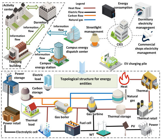
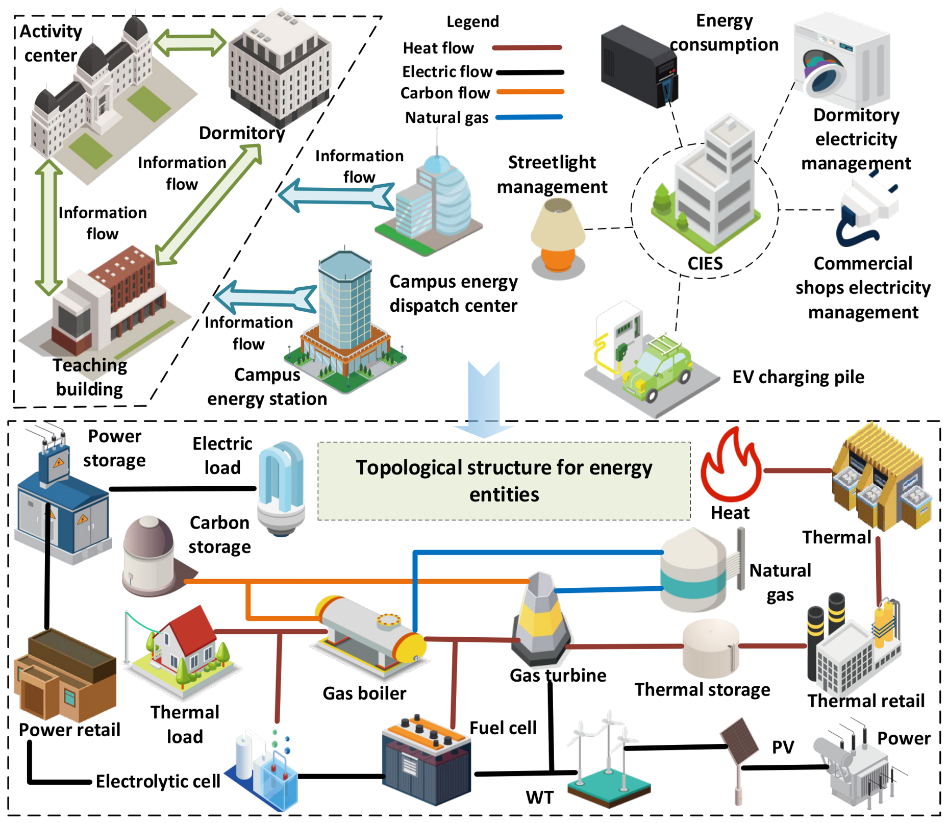
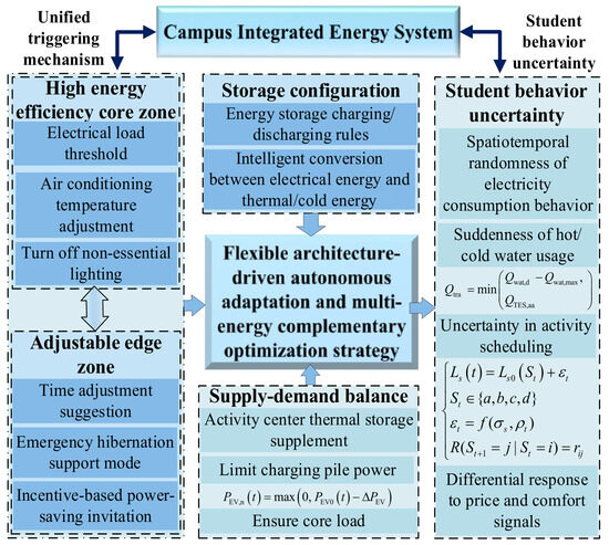
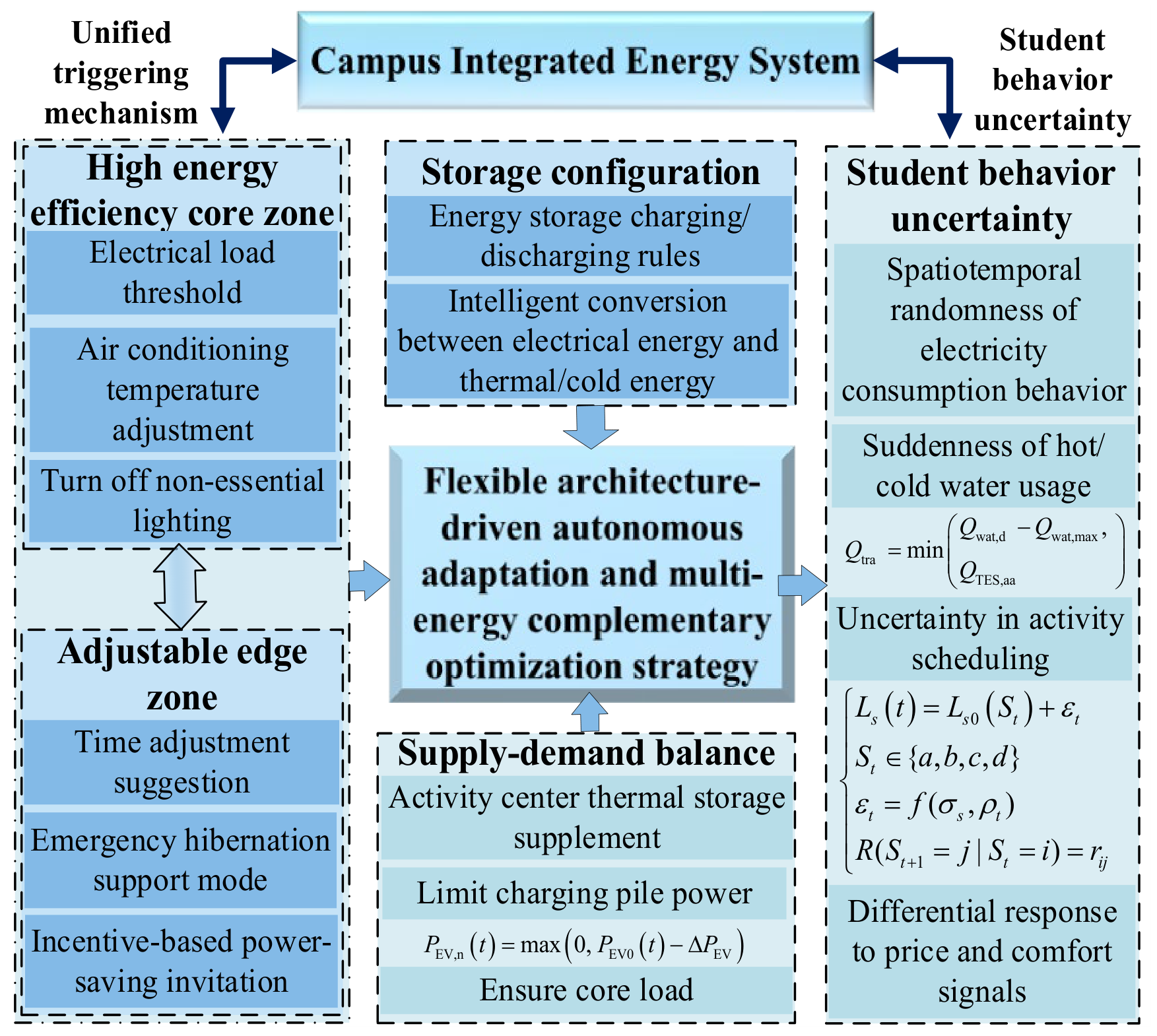
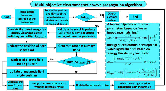
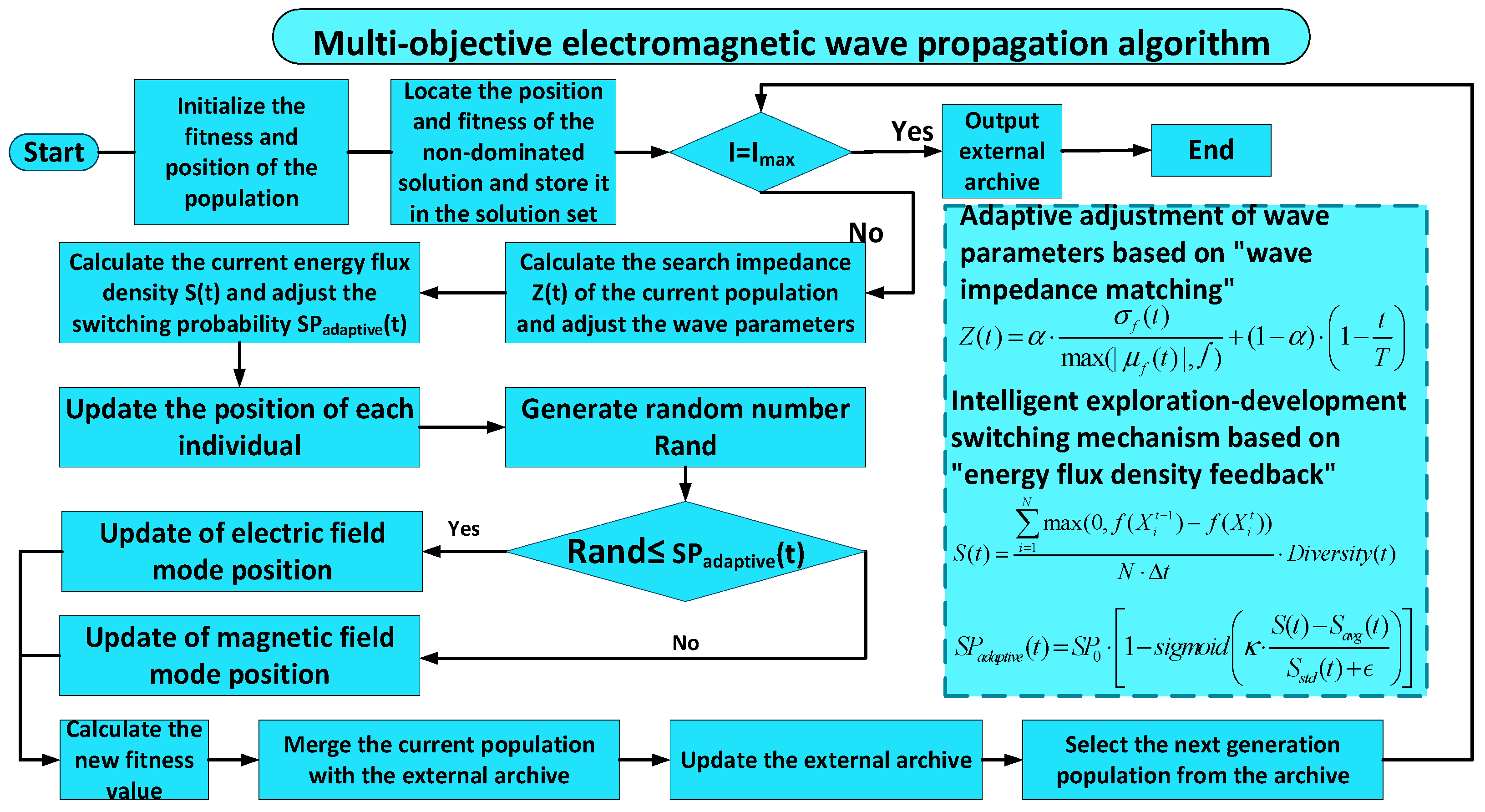
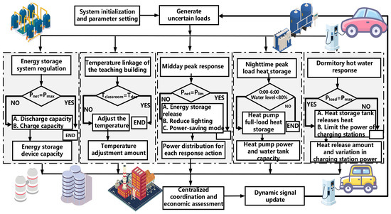
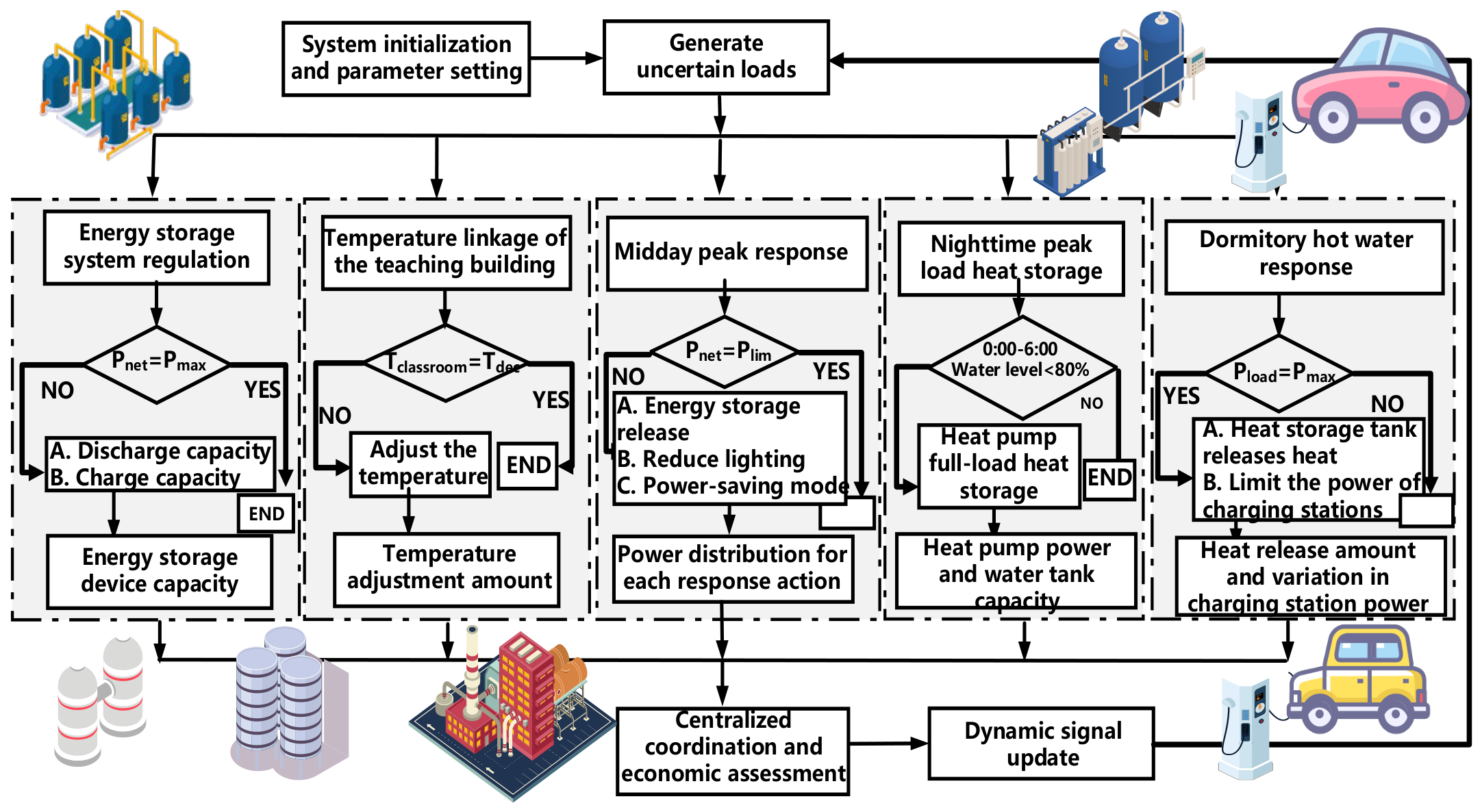
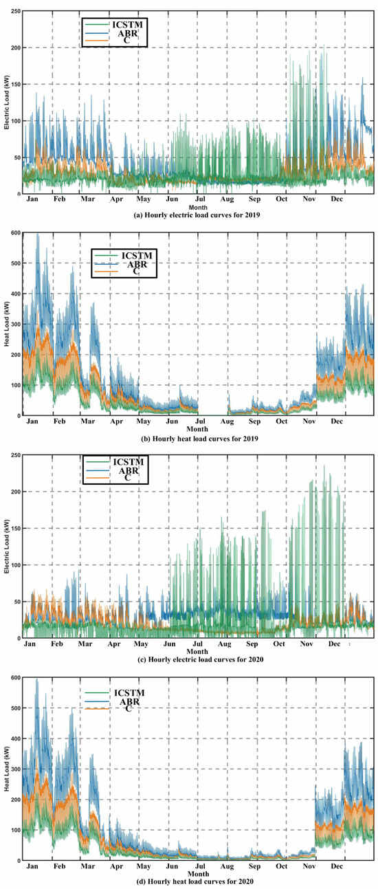
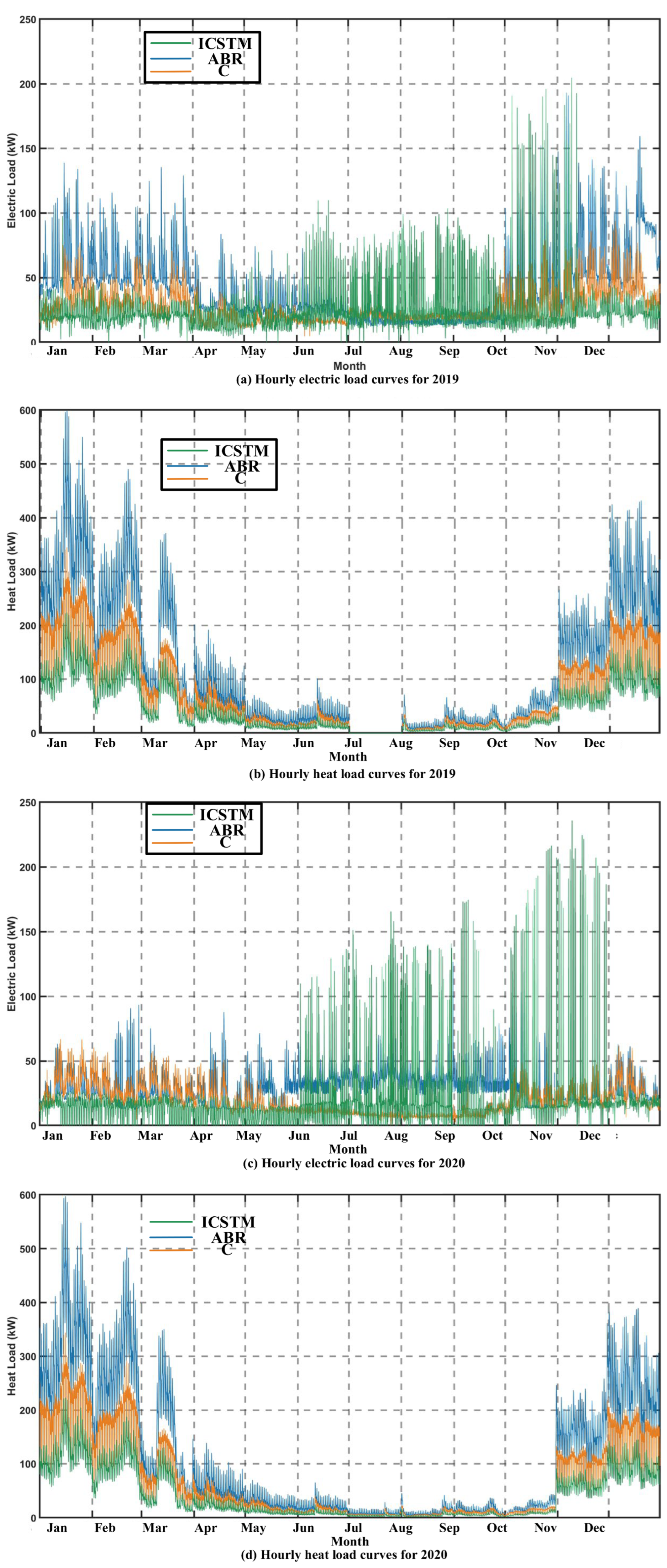
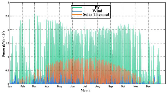
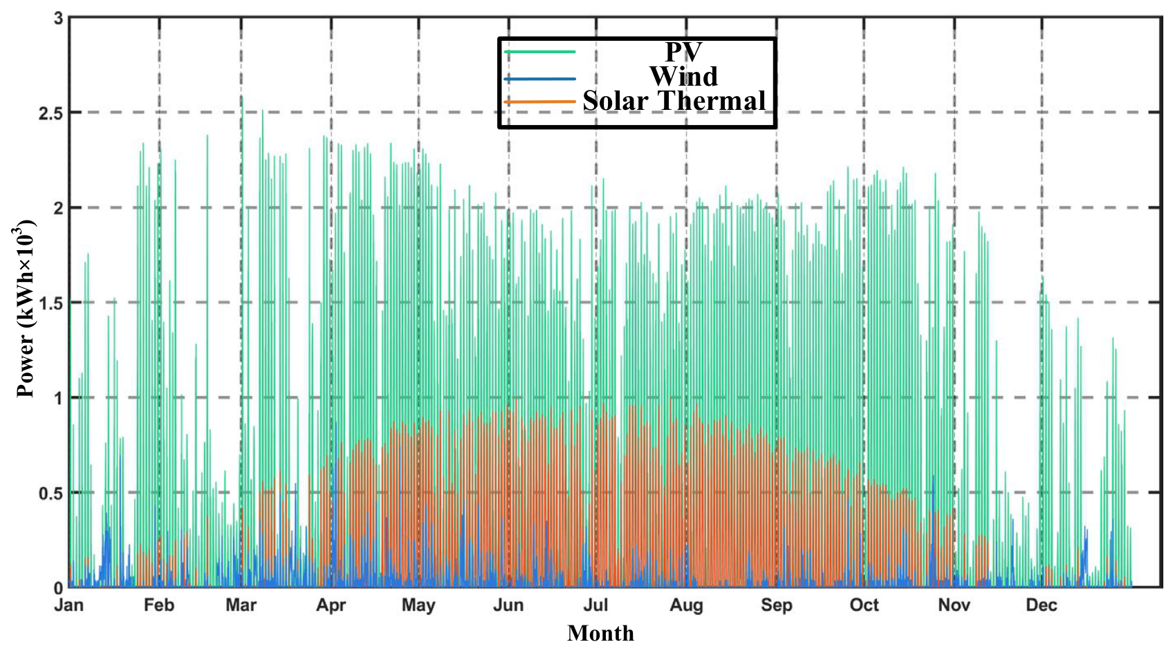
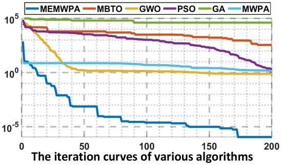
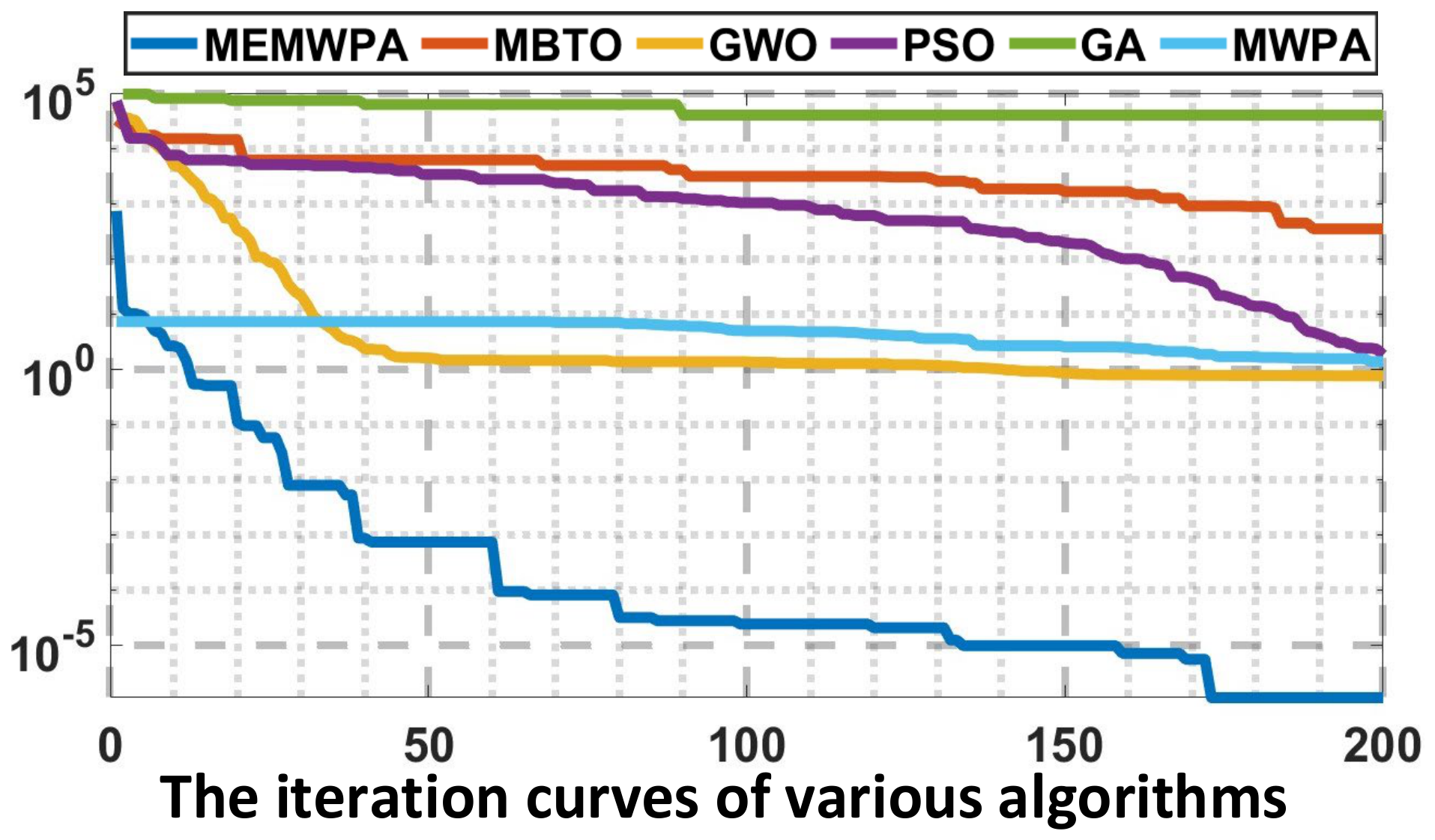
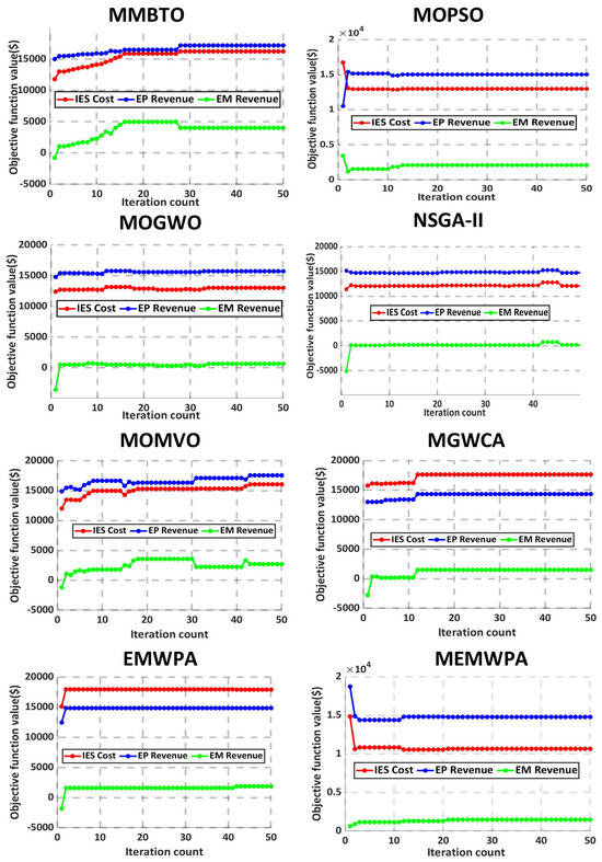
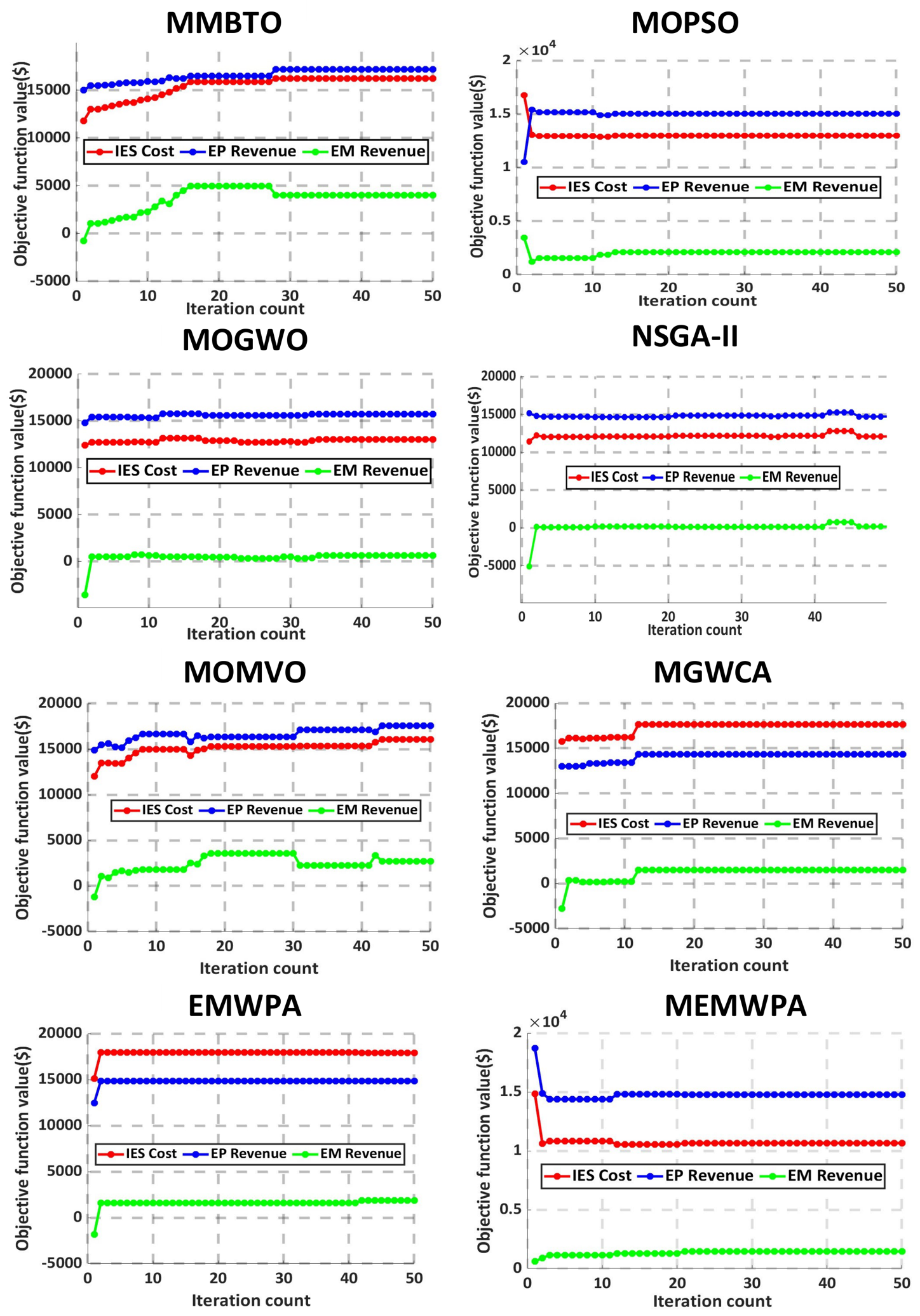
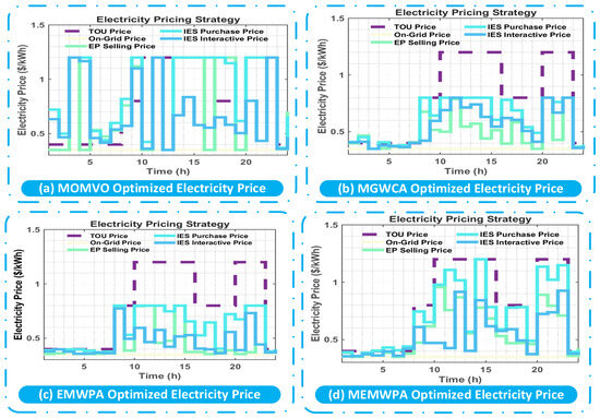
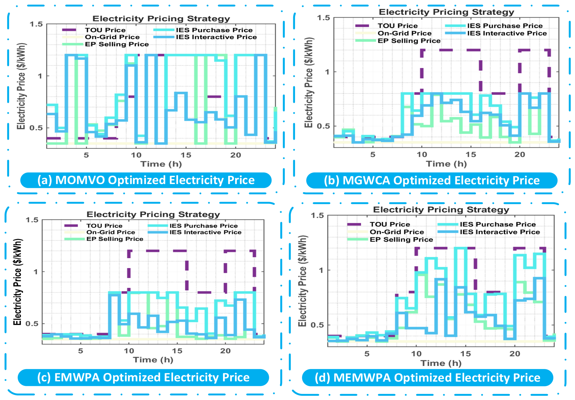
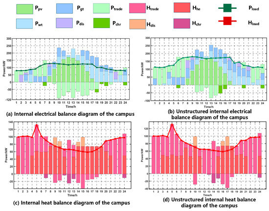
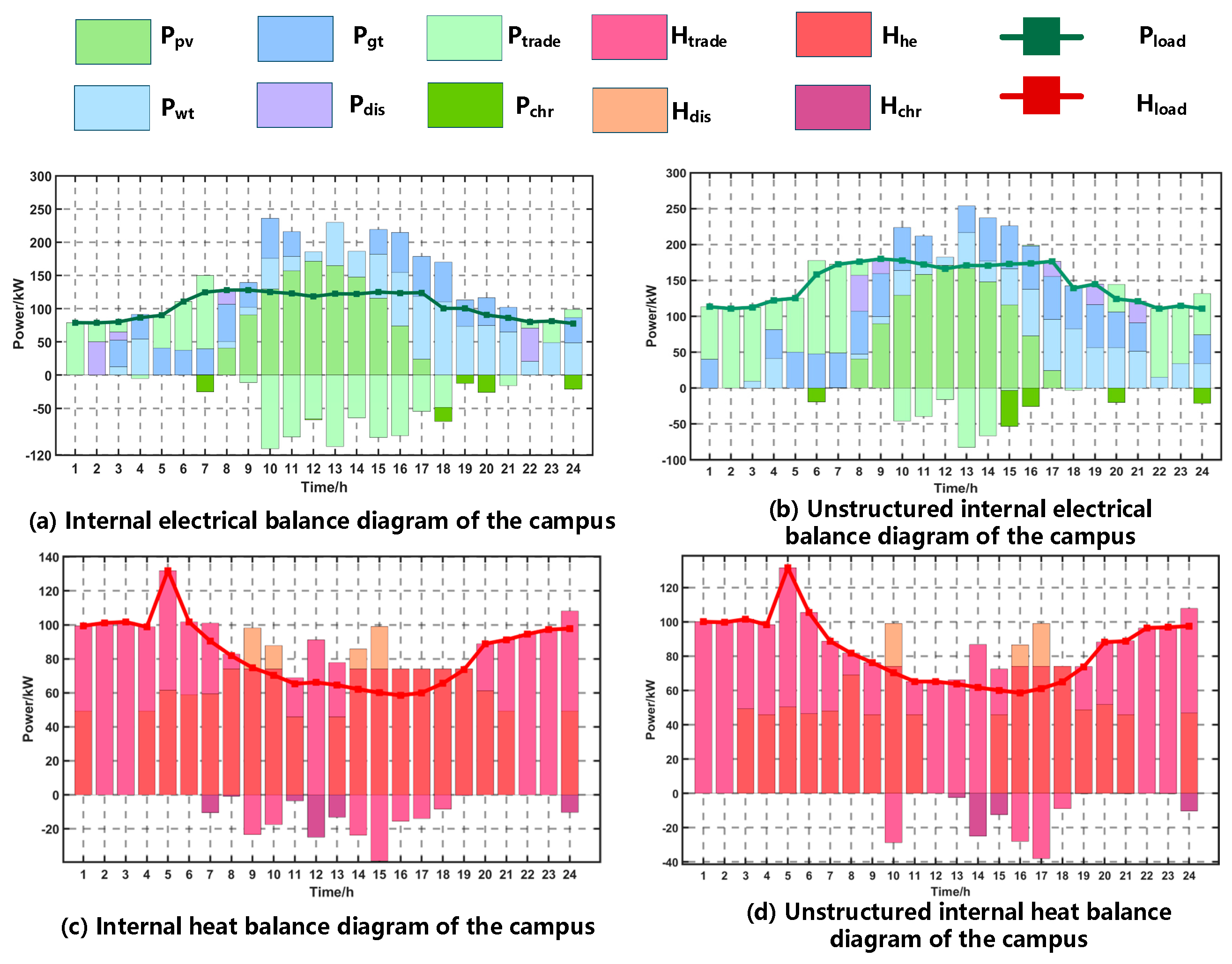
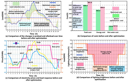
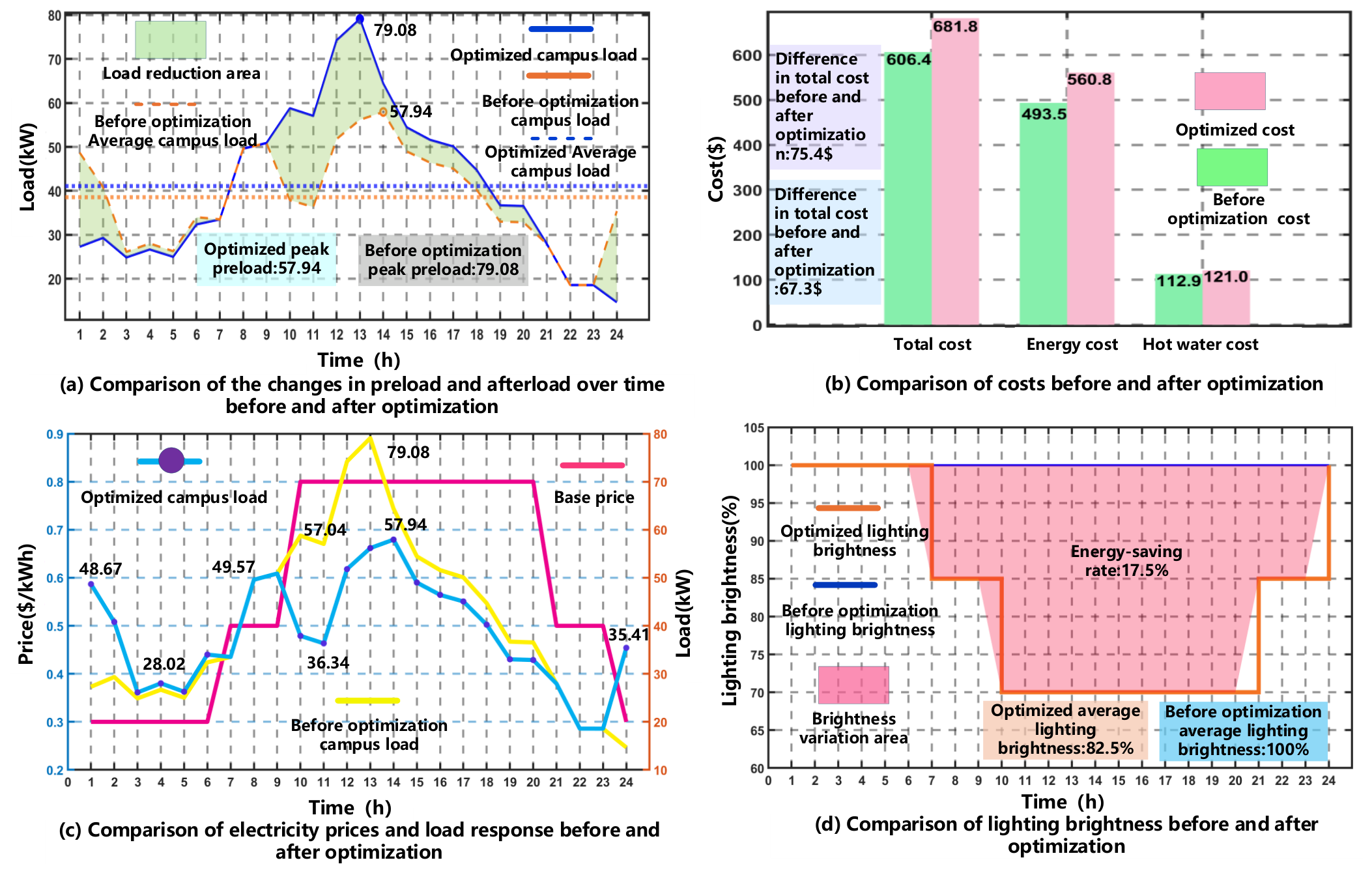
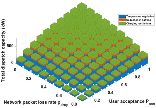
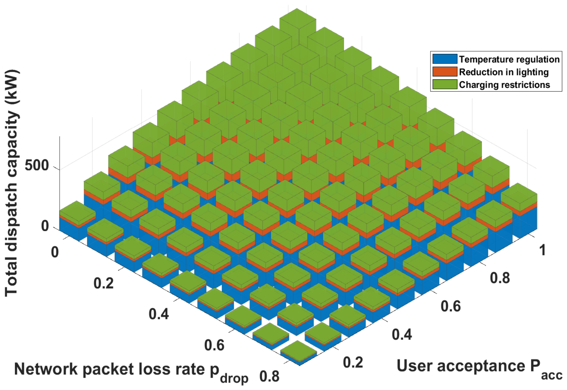
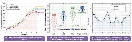
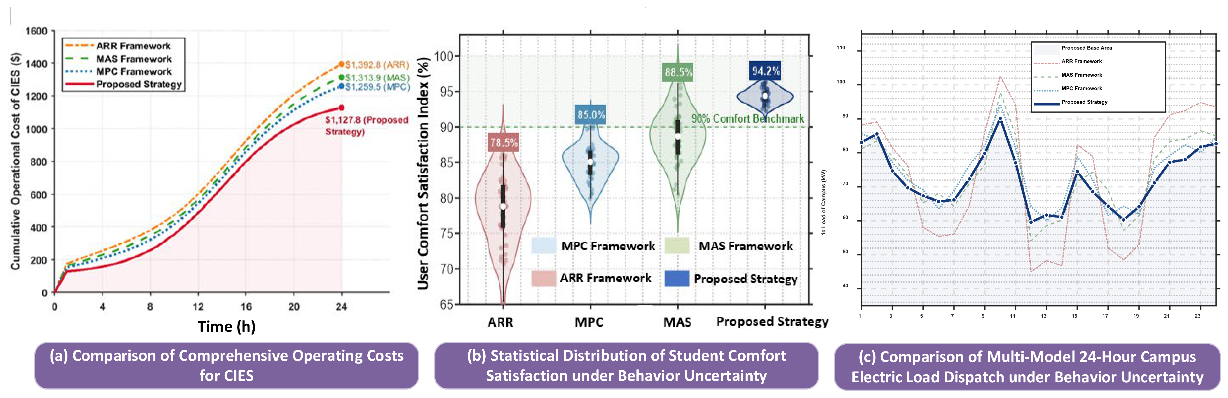
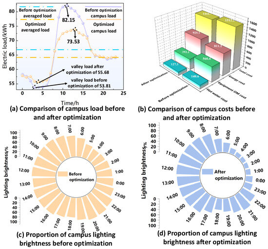
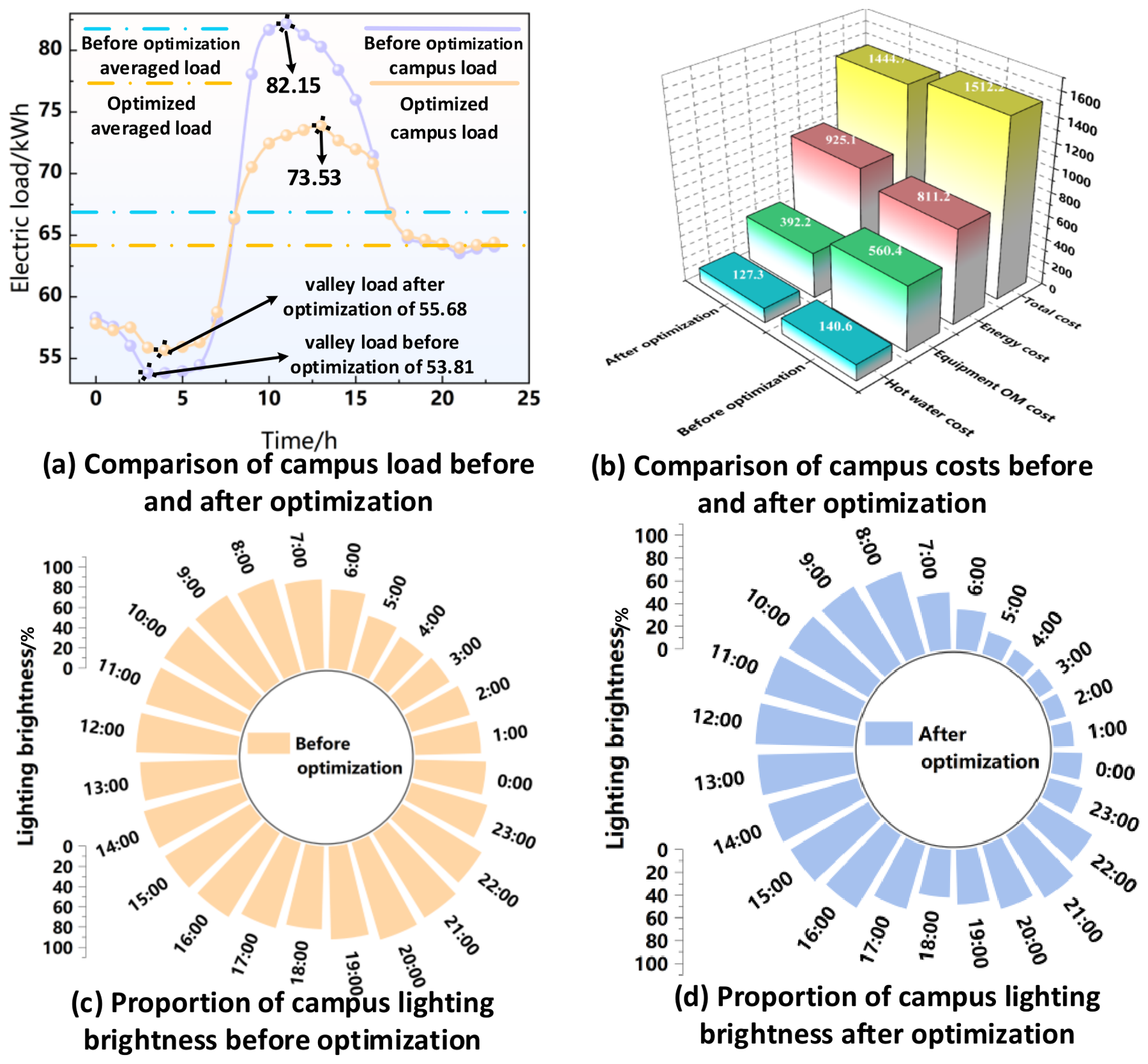
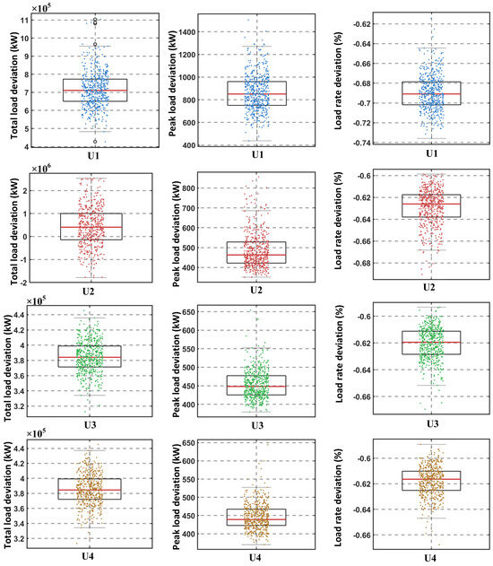
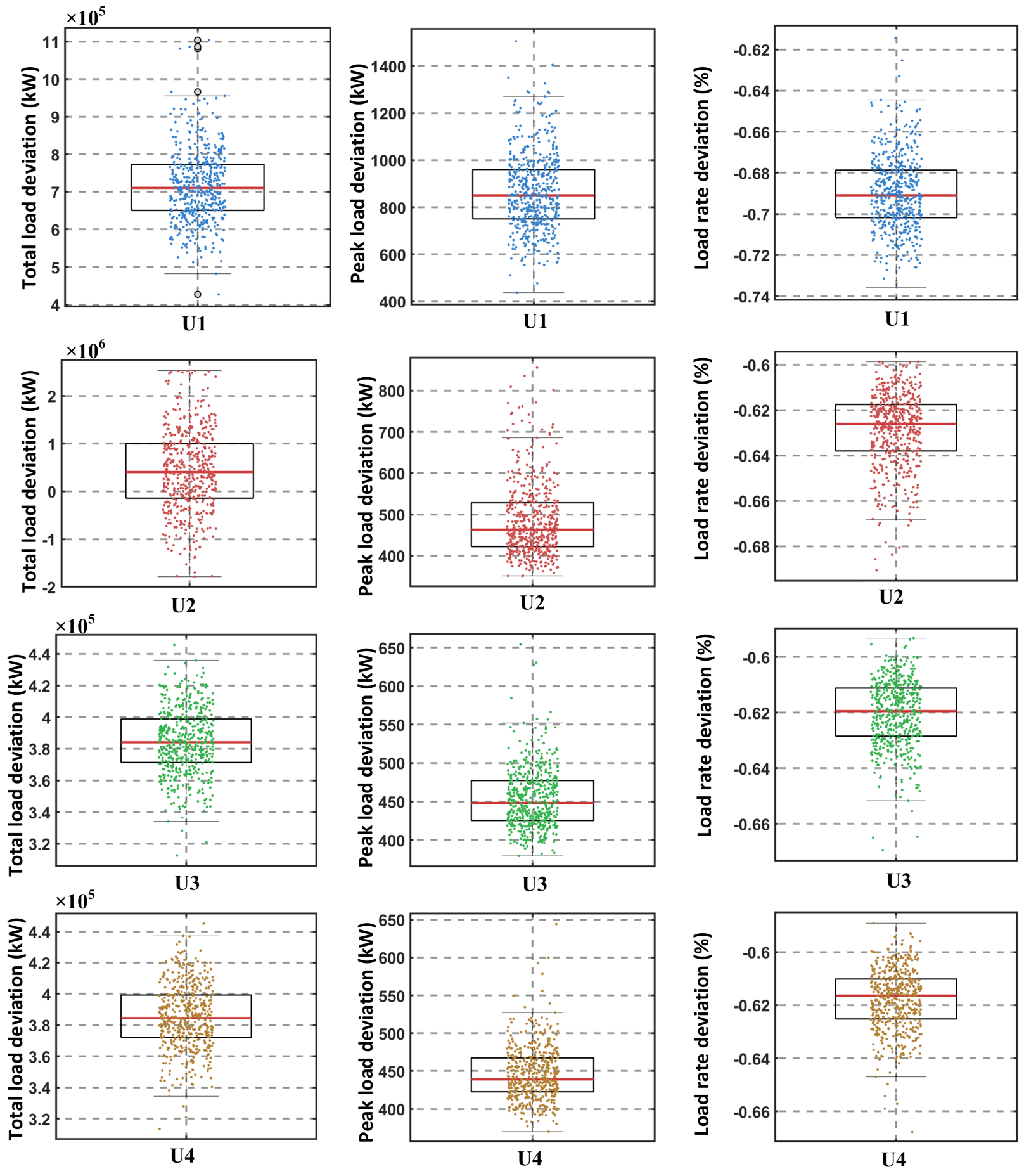
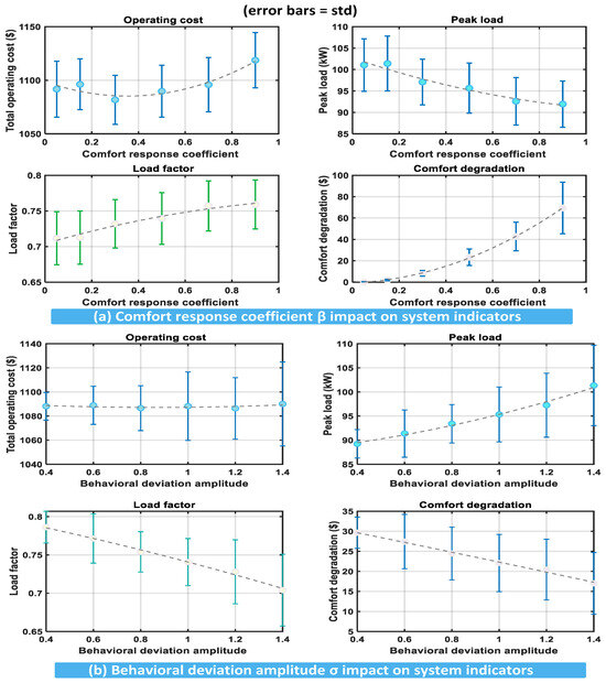
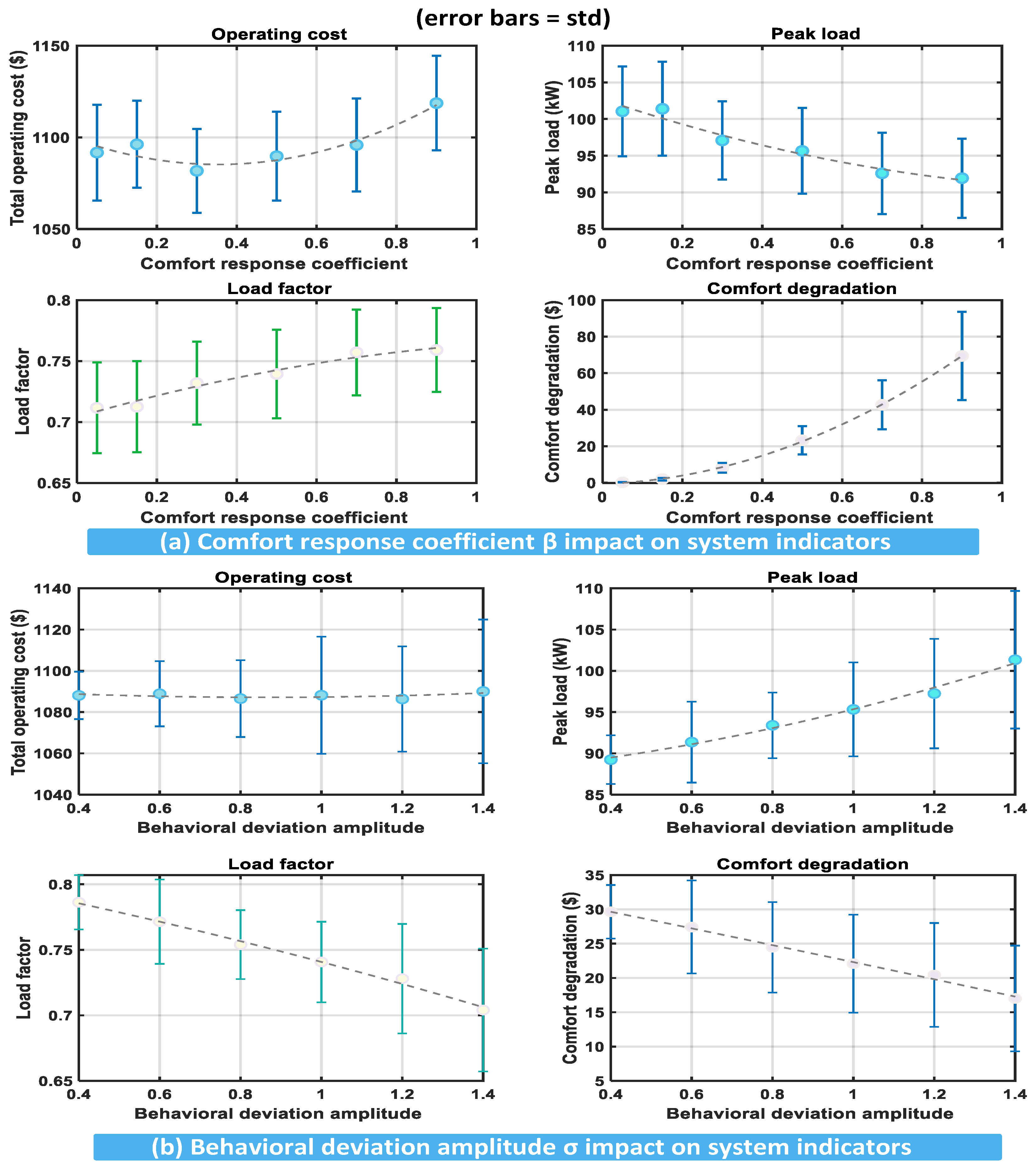
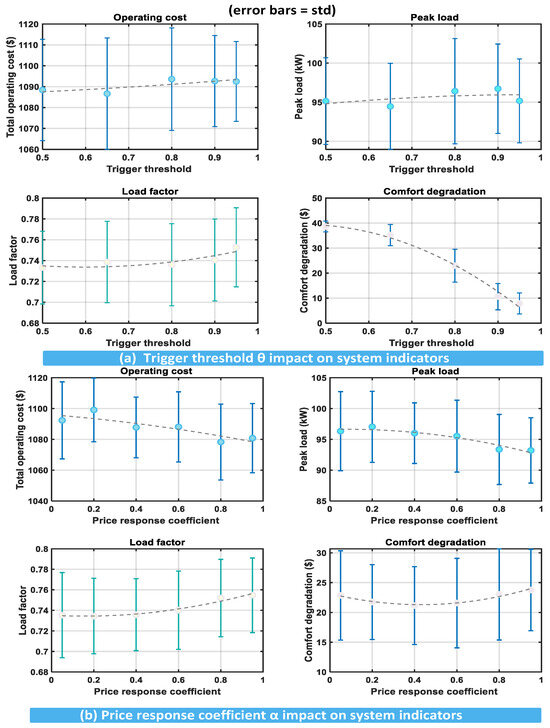
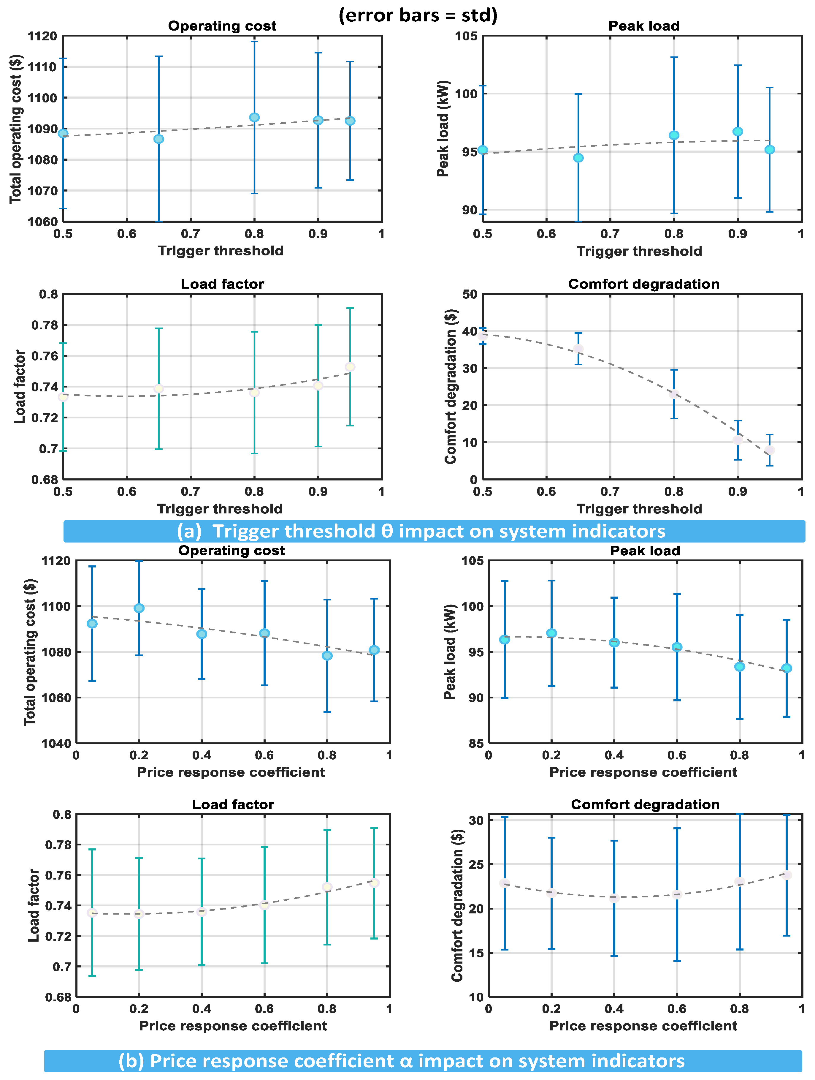
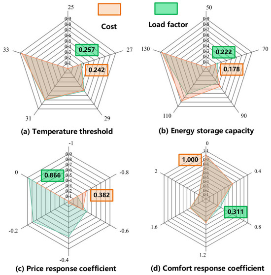
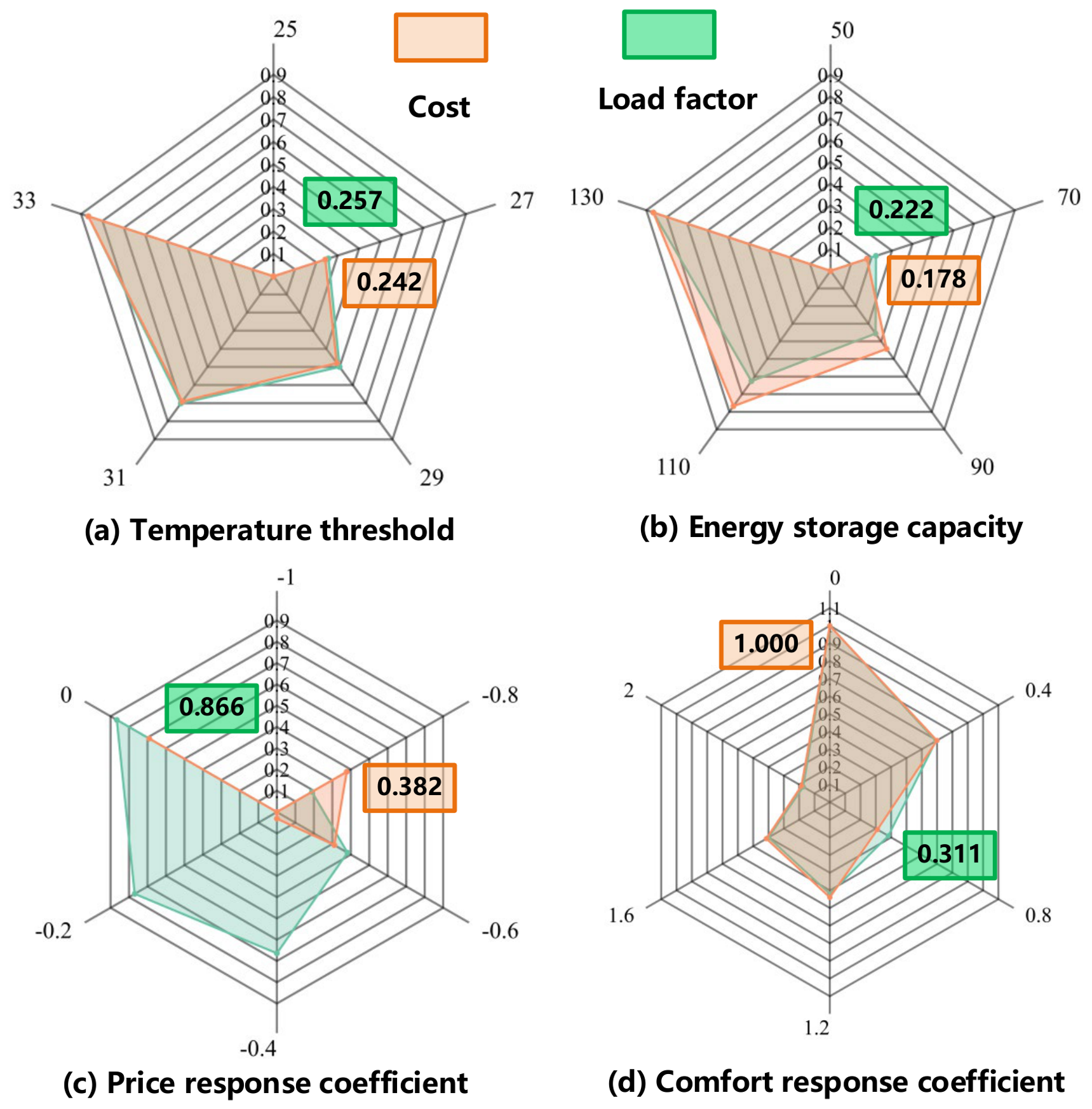
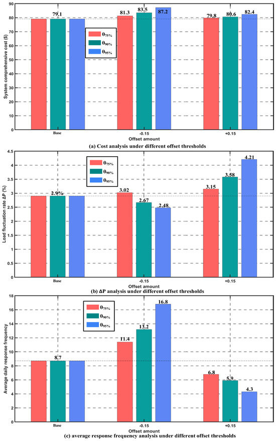
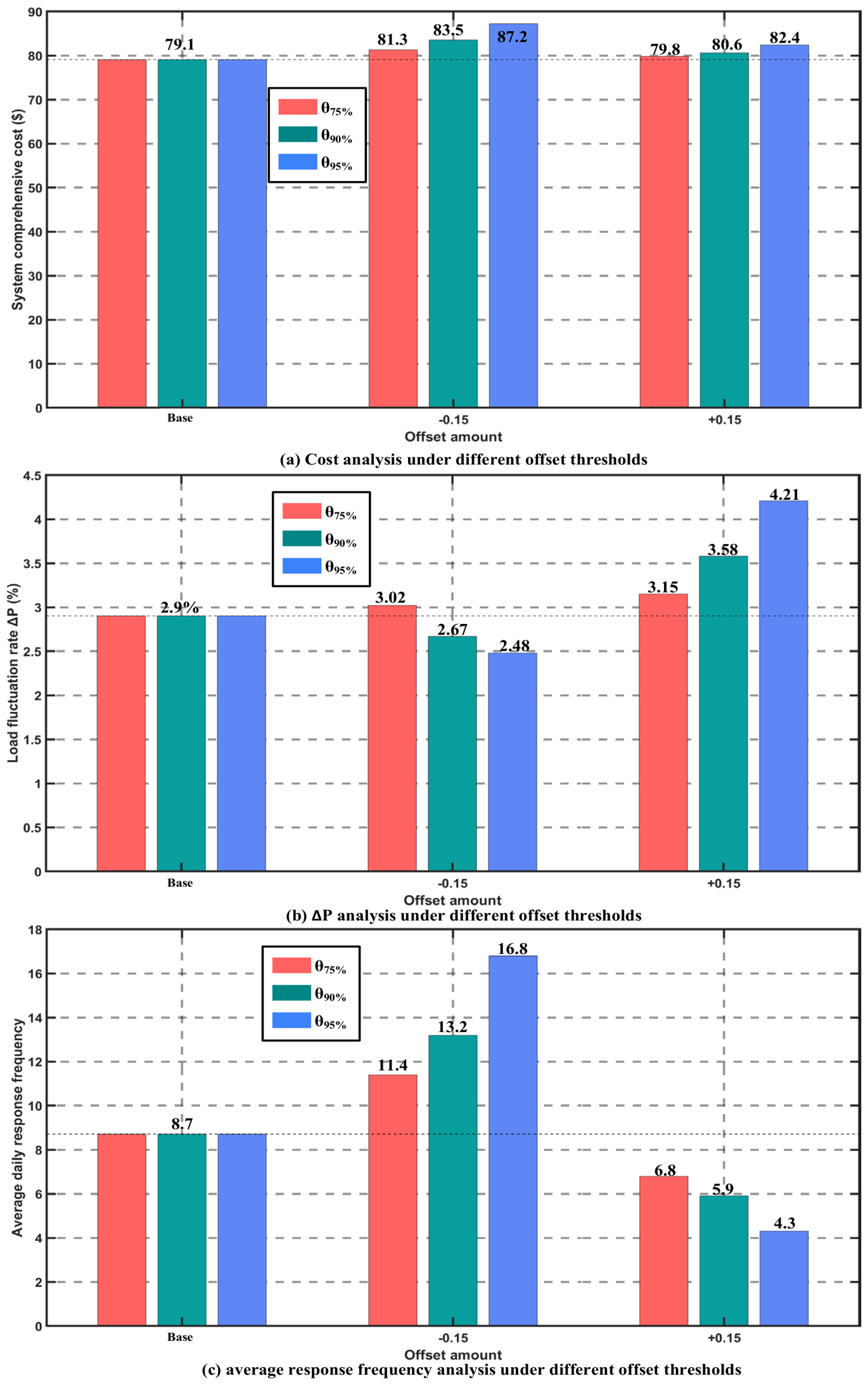

Disclaimer/Publisher’s Note: The statements, opinions and data contained in all publications are solely those of the individual author(s) and contributor(s) and not of MDPI and/or the editor(s). MDPI and/or the editor(s) disclaim responsibility for any injury to people or property resulting from any ideas, methods, instructions or products referred to in the content. |
© 2026 by the authors. Licensee MDPI, Basel, Switzerland. This article is an open access article distributed under the terms and conditions of the Creative Commons Attribution (CC BY) license.