


Abstract
This paper presents a modified two-degree-of-freedom wave buoy with an embedded tunable magnetic-spring electromagnetic energy harvester. The proposed device is modeled as a branched kinematic chain composed of a rotational–rotational buoy mechanism and a rotational–prismatic harvester branch sharing the first revolute joint. Two harvester orientations are considered and compared. The mathematical model is formulated using homogeneous transformations, velocity Jacobians and Lagrange equations. Particular attention is paid to the structure of the inertia matrix and to the way in which its inverse transmits generalized forces between the rotational coordinates and the translational motion of the moving magnet. The model is implemented in MATLAB/Simulink R2024b and evaluated under free-response, regular-wave, and bidirectional frequency-sweep excitation scenarios. Under regular-wave excitation, Config. 1 produces approximately 19.3 and 2.98 times greater average load power than Config. 2 for moving-assembly masses of 5 g and 268 g, respectively. The frequency-sweep results show that the preferred harvester orientation depends on the excitation frequency and moving-assembly mass. No resolved sweep-direction dependence is observed for 5 g, whereas for 268 g the identified hysteresis intervals are approximately 0.53 rad/s for Config. 2 and 0.64 rad/s for Config. 1. These results provide design guidelines for selecting the harvester orientation and moving mass in compact wave-excited buoy systems.
1. Introduction
Energy harvesting from ambient mechanical sources, including waves, tides, and vibrations, is increasingly considered for powering low-consumption electronic devices, wireless sensors, and autonomous monitoring systems [1,2,3,4]. In marine environments, wave-induced buoy motion represents a persistent and spatially distributed source of mechanical energy that can be used to supply onboard measurement and communication systems [1,2,3,4,5,6]. Recent research has therefore addressed hybrid triboelectric–electromagnetic and electromagnetic–piezoelectric harvesters capable of converting multidirectional buoy motion [7,8,9,10].
Electromagnetic harvesters are particularly suitable for low-frequency, relatively large-amplitude excitation [11,12,13,14,15,16]. Their operation is based on the relative motion between permanent magnets and coils, which induces an electromotive force [17,18]. Conventional wave energy converters frequently use rotational generators combined with mechanisms that transform linear motion into rotation [10]. Direct-drive linear generators offer a simpler mechanical structure but usually require operation near resonance to obtain a sufficiently large relative velocity and useful electrical output [19].
Magnetic springs provide an alternative to conventional mechanical restoring elements. Their restoring force is generated without mechanical contact through repulsive interactions between fixed and moving magnets. The resulting nonlinear force–displacement characteristic can be adjusted geometrically and may broaden or shift the effective resonance range [20,21,22]. Magnetic-spring electromagnetic harvesters have been investigated as standalone vibration-powered generators, including systems with levitated moving magnets and magnetorheological-fluid components [23,24,25]. These studies have demonstrated that the magnet arrangement, magnetic flux distribution, damping, and moving mass strongly affect the displacement response and generated power.
The integration of a nonlinear magnetic-spring harvester into a multi-degree-of-freedom floating mechanism introduces a different problem. The relative motion of the magnet is then governed not only by the local spring and electromagnetic forces but also by inertial coupling with the rotational motion of the supporting structure. In particular, the orientation of the translational guide with respect to the rotational axes may change the structure of the inertia matrix and consequently the transfer of mechanical energy to the harvester coordinate. This internal dynamic coupling has received less attention than the analysis of standalone magnetic-spring harvesters [20,21,22,23,24,25] or conventional wave-energy-converter power-take-off systems [26,27,28,29,30].
Recent studies of wave energy converter buoys have emphasized the importance of hydrodynamic modeling, hull-shape optimization, radiation damping, added mass, and wave-to-wire simulation. Numerical tools such as ANSYS AQWA, WAMIT, WEC-Sim, and computational fluid dynamics have been applied to spar buoys, point absorbers, and multi-buoy systems [31,32,33,34,35,36,37,38,39,40]. These investigations demonstrate that the absolute response and power output of a complete wave energy converter depend strongly on buoy geometry, hydrodynamic coefficients, sea state, and electrical loading.
The present study addresses a complementary and more narrowly defined problem. It investigates the internal dynamics of an embedded magnetic-spring electromagnetic harvester subjected to prescribed generalized excitations of a modified 2-DoF buoy mechanism. The model is not intended to reproduce the complete hydrodynamic interaction between a specific hull and an irregular sea state. Consequently, the results should be interpreted as the dynamic and energy-conversion characteristics of the coupled internal mechanism rather than as a direct prediction of the electrical energy production of a full-scale wave energy converter.
The proposed system consists of a spherical floating body containing a mechanism with two rotational degrees of freedom and mutually orthogonal rotation axes. A tunable magnetic-spring electromagnetic harvester is embedded in the first moving link. The relative displacement of its moving magnet introduces an additional translational coordinate, producing a three-coordinate coupled system. Two orientations of the harvester guide are considered to determine how its position relative to the rotational axes affects inertial coupling, magnet motion, and energy conversion.
The equations of motion are derived using homogeneous transformations, velocity Jacobians, and the Lagrange formalism. The nonlinear magnetic restoring force is represented by an experimentally motivated polynomial approximation, whereas energy conversion is represented by the electromagnetic transducer, described by a linear circuit with constant and , without a rectifier or power-electronic conditioning system. The response is investigated through free-decay, harmonic-excitation, frequency-sweep, and continuation analyses. Particular attention is paid to the effects of harvester orientation, effective translating mass, excitation frequency, nonlinear response branches, and the physical displacement limit of the moving magnet.
The novelty of this study lies in demonstrating that the orientation of an embedded translational magnetic-spring harvester changes the inertial structure of the coupled buoy–harvester mechanism and can produce substantially different response branches. Unlike a standalone harvester analysis, the proposed formulation captures the interaction between two orthogonal rotational coordinates and the internal translational coordinate. The bidirectional frequency sweeps with state continuation additionally indicate direction-dependent jumps and the possible coexistence of high- and low-amplitude steady-response branches.
The main contributions of this work are as follows:
- A modified 2-DoF buoy mechanism with an embedded tunable magnetic-spring electromagnetic harvester is proposed;
- A coupled three-coordinate mechanical model is derived for two orientations of the internal translational guide;
- The influence of harvester orientation, moving mass, and excitation frequency on the internal dynamic coupling is quantified;
- Frequency sweep with state continuation are used to identify enhanced-response regions, direction-dependent jump frequencies, and hysteresis intervals;
- The calculated energy-conversion indicators are evaluated together with the physical displacement constraint of the moving magnet, allowing dynamically attractive but geometrically inadmissible operating points to be distinguished.
The remainder of this paper is organized as follows. Section 2 describes the modified buoy and the embedded magnetic-spring harvester. Section 3 presents the mathematical model of the coupled mechanism. Section 4 defines the numerical model, excitation scenarios, continuation procedure, and performance indicators. Section 5 presents and discusses the numerical results, including the influence of harvester orientation, moving mass, excitation frequency, and displacement constraints. Section 6 summarizes the main conclusions, limitations, and directions for experimental validation.
2. Modified Buoy with an Embedded Magnetic-Spring Harvester
2.1. General Structure of the System
The considered system is a modified wave buoy whose floating body is represented as a hollow sphere. A two-degree-of-freedom rotary mechanism is placed inside the body; its purpose is to transform wave-induced motion into relative motion of the internal elements.
Unlike classical wave energy converters, in which the power take-off system may be connected to the seabed, to a second floating body, or to an external mechanical structure [1,2,26], the analyzed configuration assumes that the conversion mechanism is placed entirely inside the buoy. This approach is consistent with the concept of built-in wave energy converters [3].
As a result, the internal mechanism is protected from direct contact with seawater, corrosion, biofouling, and wave impacts. At the same time, the action of waves on the buoy body can be used to excite the internal kinematic chain and subsequently to excite the energy harvester located in one of its links.
In the considered configuration, the buoy is treated as a floating carrier of the mechanism. The basic internal mechanism can be represented as a serial kinematic chain composed of two revolute joints: and . The first joint is associated with the motion of the first link relative to the reference frame of the buoy, whereas the second joint describes the motion of the second link relative to the first one. The generalized coordinates of the basic mechanism are defined as:
The axes of the two revolute joints are mutually orthogonal. This arrangement enables the analysis of coupling between two rotary motion channels and makes it possible to evaluate the excitation of an additional internal translational harvester.
Figure 1 shows the concept of the buoy with an embedded mechanism in the form of a kinematic chain with two rotary degrees of freedom.
Figure 1.
Conceptual scheme of the wave buoy with an internal two-degree-of-freedom rotary mechanism: 1—free water surface/wave profile, 2—buoy body treated as a hollow sphere, 3—first revolute joint , 4—second revolute joint , 5—center of mass of the first link, 6—center of mass of the second link. The symbols and refer to the first and second links of the mechanism, respectively. The angles and describe the rotary motions in joints and .
However, the considered translational harvester should be distinguished from rotary harvesters mounted directly in the mechanism joints. If a rotary generator is coaxial with a joint and extracts energy from an existing coordinate , it does not introduce a new generalized coordinate. In that case, its influence can be represented by an additional torque, an equivalent electromagnetic damping term, and possibly an inertia reflected to the joint axis. The situation is different for a translational harvester whose translating assembly is described by an independent coordinate . If the effective mass of this assembly is not negligible, its motion affects the center of mass, the inertia matrix, and the dynamic couplings of the system, which justifies interpreting the full model as a branched kinematic chain.
2.2. Embedded Electromagnetic Harvester with a Magnetic Spring
The modification proposed in this work consists of placing the electromagnetic harvester inside the first link of the mechanism. The harvester concept is based on previous studies by the authors concerning the design, characterization, and measurements of magnetic-spring systems integrated with electromagnetic vibration generators. The harvester consists of a moving magnet, coils, and a set of permanent magnets forming a magnetic spring; the magnetic flux density distribution and the influence of the geometric parameters of the magnet–coil system on the induced voltage were previously analyzed in [23,24]. The relative motion between the magnet and the coils generates voltage according to Faraday’s law of electromagnetic induction, whereas the magnetic interaction between the permanent magnets and the moving magnet acts as a nonlinear restoring force [20,21,22,24].
The motion of the magnet is described by an additional translational coordinate Thus, in the full model, the vector of generalized coordinates of the buoy–harvester system has the form:
As a first approximation, the magnetic spring can be described by the following nonlinear polynomial relation:
where , , and denote the linear, cubic, and quintic stiffness coefficients, respectively. The corresponding restoring generalized force acting on the translating assembly is .
From the structural point of view, the analyzed harvester can be treated as a linear electromagnetic module embedded inside the first link of the mechanism. This module consists of coil assemblies and fixed relative to the link, a set of permanent magnets, and a moving magnet traveling along a local guide (Figure 2a). The guide axis is identified with the axis of the harvester branch (Figure 2b), whereas the displacement of the moving magnet relative to its nominal position is described by the coordinate (Figure 2c).
Figure 2.
Scheme of the embedded electromagnetic energy harvester with a magnetic spring and its simplified kinematic representation: (a) structural concept of the harvester with coils , , permanent magnets, and a moving magnet, (b) guide axis of the moving magnet, (c) kinematic model of the harvester as a prismatic joint .
In the considered model, the stationary harvester components, including the housing, coils, and fixed magnets, are treated as part of the first link. The translating assembly is represented by the effective mass , which includes the moving magnet, its carrier, and any additional tuning mass mechanically connected to it. The carrier and additional tuning mass are omitted from Figure 2 for clarity. The magnetic spring used in the harvester consists of a casing, upper and lower adjustment screws, and three cylindrical N38-grade NdFeB magnets: one moving magnet and two fixed magnets (Figure 3a). In the previously tested prototype, the moving magnet had a height of and a diameter of , whereas the upper and lower fixed magnets had a height and diameter of [23,24].
Figure 3.
Magnetic-spring structure: (a) disassembled components; (b) assembled magnetic spring without coil.
The moving magnet is placed inside the casing between the fixed upper and lower magnets, forming a repulsive magnetic-spring system. The fixed magnets are mounted in the upper and lower screws, which makes it possible to adjust the distance between the magnets and tune the equivalent stiffness of the magnetic spring (Figure 3b). The coil can be wound on the casing in prepared grooves. Because the repulsive magnetic force depends nonlinearly on the magnet spacing, the magnetic spring can be used to tune the dynamic response and the resonance-like operating range of the electromagnetic harvester.
2.3. Interpretation as a Branched Kinematic Chain
In the present work, the buoy–harvester system is treated as a branched kinematic chain. After including the motion of the harvester magnet, the complete system is no longer a simple serial chain (). It has a branched structure in which the first revolute joint is common to two branches: and (Figure 4). The first branch describes the basic rotary mechanism of the buoy, whereas the second branch describes the harvester motion, in which joint is a prismatic joint associated with the translation of the moving magnet (Figure 4a). In this sense, the system can be interpreted as a branched mechanism composed of a revolute–revolute branch and a revolute–prismatic branch (Figure 4b).
Figure 4.
Interpretation of the complete system as a branched kinematic chain: (a) front view, (b) side view. The main branch describes the rotary mechanism of the buoy, whereas the branch describes the harvester with the translational motion of the magnet. The first revolute joint is common to both branches.
Moreover, the equations of motion contain terms that couple the rotary motion of the first link with the translational motion of the harvester. These terms determine whether a given geometric configuration of the harvester effectively excites the motion of the magnet.
2.4. Considered Harvester-Orientation Configurations and Modeling Assumptions
Two configurations of placing the harvester in the first link of the mechanism are considered. The purpose of comparing them is to determine how the orientation of the magnet guide affects the excitation of the coordinate and, consequently, the energy-harvesting potential. Local unit vectors associated with the first link are introduced as:
The first configuration corresponds to the variant in which the center-of-mass position of the translating assembly is described as:
In this case, the translating assembly moves along the local guide axis associated with the first link (Figure 5a), and its effective distance from the first-joint axis depends on the sum . In Config. 2, the harvester guide is offset relative to the axis of the first link (Figure 5b), and the center-of-mass position of the translating assembly is described as:
Figure 5.
Considered harvester-orientation configurations in the first link of the mechanism: (a) Config. 1, for which the center-of-mass position of the translating assembly is described as , and (b) Config. 2, for which it is described as . The figure shows the differences in the orientation of the harvester guide axis and the resulting relationships between axes , , and .
Here, denotes the nominal position of the center of mass of the translating assembly along the guide axis, whereas is its displacement relative to this position. In Config. 2, the translating assembly moves along , while the constant transverse offset lies along . In Config. 1, the motion of the translating assembly primarily modifies the effective inertia of the first rotary channel, whereas Config. 2 introduces direct rotation–translation coupling. Comparing these variants makes it possible to determine which harvester orientation more effectively converts prescribed generalized excitation into relative motion of the translating assembly.
Common modeling assumptions were adopted for both configurations. The analysis focuses on the coupled dynamics of the internal buoy mechanism and the embedded harvester. Therefore, the hydrodynamic interaction between the buoy body and the surrounding water is not solved directly; instead, its effect is represented by prescribed external generalized forces acting on the rotary coordinates. No external excitation acts directly on the harvester coordinate; therefore, . The translating assembly is excited indirectly through the motion of the first link, inertial coupling, and nonlinear geometric terms. Electromagnetic energy conversion is represented by the coupled series circuit defined in Section 3.5, and the resulting coil current produces the electromagnetic reaction force acting on the harvester coordinate. Contact with mechanical end stops is not included in the equations of motion, but the calculated displacement is monitored against the admissible stroke condition . Here, denotes the maximum admissible magnitude of displacement of the translating assembly from its nominal position.
The two configurations therefore represent structurally different mechanisms of transferring rotary motion to the internal translating mass. In Config. 1, the harvester displacement modifies the effective rotary inertia, whereas Config. 2 introduces direct rotation–translation coupling. The consequences of these differences for displacement, velocity, equivalent extracted power, and the physical stroke constraint are investigated in the following sections.
3. Mathematical Model of the Coupled Buoy–Harvester System
3.1. Kinematic Description Using the D-H Convention
The mathematical model of the system was formulated in two stages. First, the kinematics were described using the Denavit–Hartenberg (D-H) notation and homogeneous transformation matrices. Second, based on the determined positions of characteristic points—the centers of mass of the links—the linear and angular velocity Jacobians, kinetic and potential energies, and equations of motion were formulated using the Lagrange formalism. The use of D-H notation requires assigning local coordinate frames to the subsequent links of the mechanism according to the rules of this convention. Axis is identified with the axis of the -th joint, whereas axis is selected so that it is perpendicular to axis and intersects it. In other words, axis is directed along the common normal between axes and . If the axes intersect, the length of this normal is zero; for parallel or skew axes, axis defines the direction of the shortest segment connecting them. Each transition between adjacent coordinate frames is described by four D-H parameters: link length , link twist , offset , and joint angle . Parameter specifies the distance between axes and measured along axis . Parameter describes the twist angle between these axes. Parameter is a displacement along axis , whereas denotes rotation about axis . For a revolute joint, the joint variable is angle , whereas for a prismatic joint, the joint variable is displacement . The considered system has the structure of a branched kinematic chain. The main branch consists of two revolute joints, and the harvester branch consists of the common first revolute joint and a prismatic joint, .
The two configurations differ in their inertial coupling between coordinates and :
Therefore, direct rotation–translation coupling occurs only in Config. 2.
The first revolute joint is common to both branches. Therefore, a single serial D-H table is not created for the whole system. Instead, the D-H parameters are listed separately for the revolute–revolute branch and for the revolute–prismatic harvester branch. Figure 6a shows the assignment of the D-H frames for harvester Config. 1. In this configuration, axis corresponds to the axis of the first revolute joint , axis to the axis of the second revolute joint , and axis to the axis of the prismatic joint . The relations are as follows: axis is perpendicular to axes and , and axis is parallel to axis . This means that in Config. 1 the moving-magnet guide axis is parallel to the axis of the second revolute joint. Variable describes the displacement of the moving magnet along axis .
Figure 6.
D-H parameters of the branched kinematic chain and for: (a) harvester Config. 1, (b) harvester Config. 2. (Red arrows indicate the coordinate axes and the positive directions of rotational and translational joint motions, whereas blue arrows indicate the geometrical D–H dimensions (link lengths and offsets).
Figure 6b shows the assignment of the D-H coordinate frames for the branched kinematic chain in harvester Config. 2. In this configuration, axis corresponds to the axis of the first revolute joint , axis to the axis of the second revolute joint , and axis is the axis of the prismatic joint of the harvester .
Parameter describes the constant offset of the harvester guide axis relative to axis , measured along the common normal according to the D-H convention. Parameter is the prismatic-joint parameter associated with the displacement of the moving magnet along axis . In the dynamic model, this displacement is described by coordinate . The D-H parameters of the main branch are listed in Table 1. This branch is common to both harvester configurations. The first row of the table corresponds to joint , and the second row to joint .
Table 1.
D-H parameters of the main branch .
The D-H parameters of the harvester branch for Config. 1 are presented in Table 2. In this configuration, the displacement of the moving magnet is collinear with the axis of the prismatic joint. The total offset along this axis is written as , where denotes the constant mounting offset and is the translational variable of the moving magnet.
Table 2.
D-H parameters of the harvester branch , Config. 1.
The D-H parameters of the harvester branch for Config. 2 are listed in Table 3. In this case, an additional geometric parameter appears; it describes the transverse offset of the harvester guide axis. Parameter defines the displacement along the axis of the prismatic joint. In the simplest case, can be assumed, whereas when the nominal position of the magnet is included, .
Table 3.
D-H parameters of the harvester branch , Config. 2.
It is worth emphasizing that in both Config. 1 and Config. 2 the origins of coordinate frames (0) and (1) are coincident and are located at joint .
3.2. Mass-Point Locations
After defining the coordinate frames and the D-H parameters, the positions of the mass points used in the subsequent dynamic model were determined. In particular, the center of mass of the first link , the center of mass of the second link , and the center of mass of the translating assembly of the harvester were defined. These positions are then used to determine position vectors, velocity Jacobians, and the kinetic and potential energies of the system. Figure 7 shows the locations of the mass points for both harvester configurations. Parameters , , and describe the positions of the centers of mass of the basic mechanism links. Parameters and refer to the center-of-mass position of the translating assembly. These quantities are not D-H parameters, but geometric parameters used to describe the positions of mass points with respect to the adopted local frames. In Config. 1, the center of mass of the translating assembly is described mainly by a displacement along the guide axis. Parameter defines the nominal position of the center of mass of the translating assembly relative to the guide, whereas describes its variable displacement. In Config. 2, the center of mass of the translating assembly requires an additional transverse parameter , because the harvester guide axis is perpendicular to axis .
Figure 7.
Positions of the centers of mass of the links for: (a) Config. 1, (b) Config. 2.
The positions of the mass points are summarized in Table 4. The parameters in this table are used only to describe the centers of mass and should not be confused with the kinematic D-H parameters listed in Table 1, Table 2 and Table 3.
Table 4.
Parameters of the center-of-mass positions.
3.3. Homogeneous Transformation Matrices
For a single transition between coordinate frames, the homogeneous transformation matrix has the form:
After expansion, this gives:
For a prismatic joint, angle is constant, while the variable parameter is . Next, using Table 1, Table 2 and Table 3, the homogeneous transformation matrices for the main branch and for the harvester branch in both configurations were determined.
For branch , the homogeneous transformation matrix from frame to the base frame has the form:
where is the homogeneous transformation matrix of frame with respect to the base frame , and matrix is the transformation from frame (E), i.e., the end of link 2 associated with joint , to frame . Matrix describes the position and orientation of the second link of the basic mechanism branch with respect to the reference frame. After multiplication, the expanded form of this matrix is obtained; due to its size, it is listed in Appendix A.1.
In Config. 1, the axis of the prismatic joint of the harvester is parallel to axis . The total displacement along the guide axis is written as:
where denotes the constant mounting offset, whereas is the translational variable of the moving magnet. The transformation matrix from the base frame to the harvester frame is:
where is the homogeneous transformation matrix of frame with respect to the base frame , and is the homogeneous transformation matrix of frame with respect to the frame . The expanded form of this matrix for Config. 1 is given in Appendix A.2. The first three elements of the last column of this matrix define the position of the harvester-frame origin; written as a transposed vector, it has the form:
where and denote the abbreviated forms of the trigonometric functions and , respectively. After substituting the expression into (13), :
This form shows that in Config. 1 the magnet motion changes the effective distance of mass from the first joint axis.
In Config. 2, the harvester guide axis is offset relative to axis . The constant offset is described by parameter , whereas the displacement along the prismatic-joint axis is described by parameter . Depending on the adopted definition of the nominal position, one can assume or, more generally The homogeneous transformation matrix for the harvester branch in Config. 2 is:
where is the homogeneous transformation matrix of frame (h) with respect to the base frame (1). The expanded form of this matrix for Config. 2 is given in Appendix A.3. In the main text, only the defining relations of the transformation and the interpretation of the parameters are retained. From the last column, the position of the harvester-frame origin is obtained:
The homogeneous transformation matrix of the first center of mass of branch has the form:
where is the homogeneous transformation matrix from frame to the base frame . The expanded form of matrix is presented in Appendix A.4. The homogeneous transformation matrix of the second center of mass of branch has the form:
where is the homogeneous transformation matrix from frame to the base frame . For the second link, the position of the center of mass was determined using the transformation:
with angle . Parameter from Figure 7a is further identified with parameter used in the dynamic equations. The expanded form of matrix is presented in Appendix A.5. The homogeneous transformation matrix of the harvester center of mass for branch , for Config. 1, has the form:
where is the homogeneous transformation matrix of the harvester center of mass from frame to the base frame , for Config. 1. The expanded form of matrix is presented in Appendix A.6. The homogeneous transformation matrix of the harvester center of mass for branch , for Config. 2, has the form:
where is the homogeneous transformation matrix of the harvester center of mass from frame to the base frame , for Config. 2. The expanded form of matrix is presented in Appendix A.7. The last columns of matrices , , , and define the position vectors of the mass points—the centers of mass , , , and in the base frame. On this basis, the linear velocity Jacobians can be determined:
and, for the rotary links, the angular velocity Jacobians:
where denotes the linear velocity Jacobian of the i-th center of mass, is the angular velocity Jacobian of the i-th link and of the corresponding center of mass, is the vector of joint variables, and is the derivative of the vector of joint variables. These Jacobians are then used to determine the kinetic energy of the system and the inertia matrix. For the center of mass of the first link , only the first revolute joint is active; therefore:
where is the coordinate vector of the origin of the base coordinate frame, is the position vector of the center of the link, and is the unit vector of axis of the base coordinate frame. The expanded Jacobians for point are listed in Appendix B.1. For the center of mass of the second link , joints and are active, whereas the prismatic joint of the harvester does not affect the motion of this point. Thus:
where is the coordinate vector of the origin of coordinate frame , is the position vector of the center of the link, and is the unit vector of axis of coordinate frame . The expanded Jacobians for point are listed in Appendix B.2.
For the center of mass of the translating assembly , the common revolute joint and the prismatic joint are active. The second revolute joint is not located on the branch leading to the translating assembly; therefore, its corresponding Jacobian column is zero. For configuration , one can write:
The expanded linear Jacobians of the translating assembly for both configurations are listed in Appendix B.3. If the assembly is represented by an effective point mass moving along the guide, its contribution to the kinetic energy can be described using the linear Jacobian. If its rotational inertia transported with the first link is also included, one may assume:
The corresponding angular Jacobians of the translating assembly are listed in Appendix B.4. The obtained Jacobians are then used to formulate the kinetic energy of the system.
3.4. Energies, Inertia Matrix and Nonlinear Terms
Based on the Jacobians defined in the previous subsection, the kinetic energy of the system can be written as:
where denotes the harvester configuration number.
Consequently, the inertia matrix of the system can be written as:
This formulation directly shows that the differences between Config. 1 and Config. 2 result primarily from the different form of the Jacobian , i.e., from the different geometry of the motion of the center of mass of the translating assembly . The form of the inertia matrix including only the contribution of the main branch is:
where , , .
The general structures of the inertia matrix for the two harvester configurations are then:
This form shows that in Config. 1 the translational channel is not directly inertially coupled with the rotary channels. In Config. 2, however, an additional element appears as a result of the transverse position of the center of mass of the translating assembly. The inertia matrices for Config. 1 and Config. 2 are as follows:
The block structure of the inertia matrix has a direct physical interpretation. The diagonal terms describe the self-inertia of the main rotary mechanism and of the translating assembly, whereas the off-diagonal terms describe inertial coupling between the generalized coordinates. Similar block-matrix descriptions were previously used for mechatronic systems and robot-like mechanisms, where the internal structure of the inertia matrix was related to the topology of the kinematic chain [41,42,43].
The vector of centrifugal and Coriolis terms was determined from the Christoffel symbols. For the elements of the inertia matrix , the notation is adopted as:
For branch , after including the shift in the description of , one obtains:
The contribution of the translating assembly for Config. 1 is:
For Config. 2, the terms resulting from the variability of have an analogous form. The constant parameter affects the inertia matrix through element , but does not generate additional configuration derivatives in .
The potential energy of the system is the sum of the gravitational energy of the main branch, the gravitational energy of the translating assembly, and the magnetic-spring energy. Since gravity acts along the axis, the potential energy depends on the second component of the position vectors of the mass points. For the main branch:
The contribution of the translating assembly is, respectively:
The total potential energy and the vector of potential forces are therefore:
For the main branch, one obtains:
After adding the harvester contribution, one obtains, respectively:
3.5. Equations of Motion and Simulation Form
After determining the inertia matrix, the centrifugal and Coriolis terms, the potential-force vector, and the damping vector, the equations of motion of the system can be written in compact form:
where denotes harvester Config. 1 or 2, is the vector of transducer torques/forces, is the vector of external excitations, and is the damping vector. The damping vector has the form:
where and are the damping coefficients in the joints, and friction associated with the motion of the magnet in the guide was described using a continuous, velocity-dependent Coulomb–Stribeck [44] model supplemented with a linear viscous term:
where denotes the Coulomb friction force, is the characteristic force in the low-velocity region and at the onset of sliding, determines the decay rate of the Stribeck effect, controls the smoothing of the force sign reversal in the vicinity of , and is the viscous loss coefficient.
After moving the state-dependent terms to the right-hand side, one obtains:
where .
Formally, this can be written as:
However, in the MATLAB/Simulink implementation, the inverse matrix is not explicitly formed. Instead, the linear system is solved using the left-division operator.
To account for the electrical dynamics of the electromagnetic generator, the coil current was introduced as an additional state variable. Consequently, the extended state vector and the coupled electromechanical model are expressed as:
Here, denotes the harvester configuration. In the sign convention adopted in Equation (51), the electromagnetic generalized-force vector is . Equivalently, the implementation may include as a positive resistance term on the left-hand side of the translational equation. The vector includes the electromagnetic reaction force acting on the moving magnet:
where is the force coefficient of the generator. The negative sign indicates that the electromagnetic force opposes the motion of the magnet. For a reciprocal electromagnetic transducer expressed in SI units, .
The instantaneous power delivered to the resistive load and its mean value over the time interval [, ] are calculated as:
In the steady-state analyses, the averaging interval [, ] corresponds to the final 20 excitation periods.
4. Numerical Simulation of the Buoy Models
The system concept presented in Section 2 and the mathematical models derived in Section 3 were implemented in MATLAB/Simulink. The implementation structure is shown in Figure 8. The presented scheme corresponds to the buoy–harvester system for Config. 1, in which the axis of the prismatic joint of the harvester is parallel to axis of the main branch . The model of the second configuration, in which the prismatic-joint axis is perpendicular to axis , has an analogous block structure. The difference between the configurations occurs inside the main computational MATLAB Function block, where the appropriate forms of the inertia matrix , the centrifugal and Coriolis vector , the potential-force vector , and the geometry of the harvester branch are implemented.
Figure 8.
Implementation scheme of the buoy–harvester model in MATLAB/Simulink. The structure includes a wave-excitation generator, a parameter block, the main dynamics block, and a subsystem integrating the state vector. The same architecture was used for both harvester configurations.
The state signal is fed back from the integration subsystem to the main dynamics block and to the wave-excitation generator. Simulation time is provided by the clock block and is used both for generating time-dependent excitations and for computing the equations of motion. The init_boja_wave_u_params block initializes the wave-excitation parameter vector . Its inputs and are approximate effective moments of inertia of the and channels, respectively, and are used to calculate the equivalent wave-coupling stiffness and damping coefficients. The load-case identifier is supplied separately to the boja_harwester_wave_u block as caseID. The regular-wave excitation was represented by an equivalent prescribed angular motion acting on the first rotational coordinate through a linear spring–damper coupling. For a monochromatic deep-water wave, the surface elevation, angular frequency, and wave number are defined as:
where is the wave height and is the wave period. Using the local-wave-slope approximation, the equivalent angular excitation is expressed as:
The corresponding generalized excitation vector is given by:
where and are the equivalent stiffness and damping coefficients describing the wave-induced coupling with the first link, respectively. The quantities and denote the equilibrium angular position and the corresponding balancing torque. Thus, the wave excitation is introduced as an equivalent kinematic input rather than as a directly prescribed harmonic hydrodynamic torque. For the regular-wave case considered in this study, and , which correspond to , , and .
In extended variants, the second rotary axis may also be excited in order to analyze the response of the system to more complex or spatial wave interaction.
This means that the magnet motion is excited indirectly by the motion of the buoy mechanism, inertial couplings, and nonlinear terms resulting from the system geometry. The waveOut output is diagnostic and may contain auxiliary information about the excitation, such as the current value of the wave moment, frequency, amplitude, or other parameters of the excitation signal. The sources block assembles the input signals of the dynamic model. The input vector of the dynamics block has the form:
The components are reserved for optional transducer forces, moments, or additional test inputs. In the simulations reported here, these external transducer inputs were set to zero. The electromagnetic reaction was evaluated internally from the coil-current state; in the convention of Equation (51), it is represented by . The model-parameter vector contains the mechanical, geometric, magnetic-spring, friction, and electrical parameters listed in Appendix C. The instantaneous and average load powers are calculated from the simulated current using . In particular, this block defines the parameters of the main branch , the translating assembly parameters, and the values , , and , which affect the harvester response and the calculated harvested power.
The main MATLAB Function block performs the computations of the dynamic model. At each simulation step, this block evaluates the inertia matrix , the velocity-dependent vector , the potential-force vector , the damping vector , the generalized force vector , and the right-hand side of the equations of motion:
The generalized accelerations are computed by solving the linear system:
In the implementation, the inverse matrix is not explicitly calculated, which improves numerical stability and is consistent with standard MATLAB practice. The output of the main block is the state derivative:
This signal is passed to the Integrators subsystem, where accelerations are integrated to velocities and then velocities are integrated to generalized coordinates. In this way, a closed simulation loop is formed. The remaining outputs of the MATLAB Function block, such as , , , , , rhs, Reac, and diagOut, are diagnostic. They enable verification of the computations, analysis of the inertia-matrix structure, checking of potential and damping forces, evaluation of joint reactions, and monitoring of selected auxiliary quantities, such as the effective magnet position, determinant of the inertia matrix, or axial force in the harvester.
4.1. Simulation Study Program
After the model implementation, the numerical study was divided into three stages. The first stage was a free-response test under gravity, aimed at verifying the correctness of the couplings between joints , , and the translational coordinate of the harvester . No external wave excitation was applied in this test; the motion of the system resulted from the initial conditions and gravitational forces. This test made it possible to check whether the deflection of the first link leads to the expected response of the second joint and whether the motion of the basic mechanism is transferred to the moving magnet.
The second stage analyzed the response of the system to a regular wave. The excitation was introduced as a generalized moment acting mainly on the first rotary channel.
Both harvester configurations were compared for two values of the effective translating mass: and . The purpose of this stage was to determine which configuration more effectively converts the rotary motion of the mechanism into relative magnet motion and how the change in the effective translating mass affects the response , the velocity , the average harvested power, and the energy.
Two moving-mass variants were considered: , representing the original lightweight configuration, and , corresponding to the physically realizable modified moving assembly. The substantially increased mass was introduced to investigate whether the resulting change in inertia could shift the harvester resonance toward the considered wave-excitation frequency range. Therefore, the value represents a construction-based parameter rather than an arbitrarily selected or numerically optimized value.
The third stage involved a frequency sweep of the excitation. For each frequency, the responses of both configurations were calculated and energy-performance indicators were determined. Particular attention was paid to the RMS velocity of the moving magnet because the instantaneous power harvested by:
The average power was also considered:
and the recovered energy:
The indicators were calculated after removing the transient state, within a fixed time window covering the final 20 excitation periods. Thus, the comparison of configurations was based on the quasi-steady response rather than on transient effects caused by the initial conditions.
4.2. Free-Response Test Under Gravity
In this test, the correctness of the model was verified for zero excitations and the following initial conditions:
which produced free motion of the kinematic-chain links. Figure 9 shows the time histories of the displacements and joint velocities during the initial motion phase up to 5 s.
Figure 9.
Free-decay responses of the system without wave excitation for Configurations 1 and 2 and two moving-assembly masses and , obtained using the fifth-order polynomial model of the magnetic spring. The initial conditions were , with all remaining state variables initially equal to zero.
The free-response histories presented in Figure 9 show that the rotational coordinates of all four system variants approach their respective static equilibrium positions within the simulated interval. The translational response, however, is strongly dependent on the moving-assembly mass. For , the moving-assembly oscillations decay substantially within 5 s, whereas for , residual translational oscillations are still visible at the end of the simulated interval. Config. 1 transfers a larger portion of the initial rotary motion to the moving assembly and therefore produces greater translational displacement and velocity amplitudes than Config. 2. Increasing the moving-assembly mass reduces the oscillation frequency and prolongs the transient response, which is consistent with the increased inertia of the translating assembly. For , the peak value of reaches approximately 19 mm and therefore exceeds the assumed physical stroke limit . Consequently, this trajectory should be interpreted as a numerical free-response verification of the unconstrained smooth model rather than as a physically admissible motion of the prototype, because end-stop interactions are not included in the present model. Figure 9 confirms the expected transfer of motion between the rotary and translational coordinates, but the finite simulation interval does not provide a formal proof of asymptotic stability. Since no external wave excitation is applied in this test, power-based performance indicators are not evaluated.
4.3. Regular-Wave Test
In this test, the system was excited by a regular wave with a period of and a wave height of . Figure 10 presents the mean-removed moving-assembly displacement and the moving-assembly velocity over the final 20 excitation periods. Config. 1 produces greater translational response amplitudes for both moving-assembly masses, although the difference between the configurations depends strongly on .
Figure 10.
Time histories of the dynamic moving-assembly displacement and moving-assembly velocity under regular-wave excitation: (a) , (b) . Solid lines denote Config. 1 and dashed lines denote Config. 2. The final 20 excitation periods are shown.
Figure 11 compares the average load power and the moving-assembly RMS velocity. Table 5 lists the corresponding response indicators, whereas Table 6 reports the ratios obtained for Config. 1 relative to Config. 2. The values of were smaller than the adopted reporting precision and are therefore displayed as zero; they should not be interpreted as identically zero.
Figure 11.
Comparison of regular-wave response indicators: (a) average load power and (b) RMS velocity of the moving assembly.
Table 5.
Response and energy indicators under regular-wave excitation. The metrics were evaluated over the final 20 excitation periods after removal of the transient response. The RMS displacements of the rotational and translational coordinates were calculated from their mean-removed components.
Table 6.
Ratios of regular-wave response indicators obtained for Config. 1 relative to Config. 2.
Under regular-wave excitation, the influence of the harvester orientation depends strongly on the moving-assembly mass. For , the dynamic RMS responses of the first rotational coordinate are nearly identical for the two configurations, whereas Config. 1 produces approximately 4.35 times greater RMS displacement and 4.38 times greater RMS velocity of the moving assembly than Config. 2. With the complete electrical generator model, the greater translational velocity produces a larger induced current and results in approximately 19.3 times greater average load power in Config. 1. This power ratio is close to the square of the velocity ratio, consistent with the circuit equation and the instantaneous load–power relationship . For , the advantage of Config. 1 is reduced but remains evident. Its moving-assembly RMS displacement and velocity are approximately 1.15 and 1.73 times those obtained for Config. 2, respectively, while its average load power is approximately 2.98 times greater.
Increasing the moving-assembly mass from 5 g to 268 g substantially enhances the translational response of both configurations. The moving-assembly RMS velocity increases by factors of approximately 28 and 71 for Config. 1 and Config. 2, respectively. The corresponding average load power increases from 0.888 to 699.46 for Config. 1 and from 0.046 to 234.73 for Config. 2.
These results demonstrate that the increased moving-assembly mass enhances the harvester response under the considered regular-wave excitation. However, the regular-wave test corresponds to an angular excitation amplitude of , whereas the frequency sweeps presented in Section 4.4 were performed with an amplitude of 0.2 rad. Because the coupled buoy–harvester system is nonlinear, its frequency response and transition frequencies may depend on the excitation amplitude. The frequency-sweep results can therefore be used to compare the two configurations and identify transition regions for an excitation amplitude of 0.2 rad, but they should not be interpreted as directly locating the resonance of the regular-wave case.
4.4. Excitation Frequency Sweep Test
To determine the excitation-frequency ranges in which each harvester configuration is more advantageous, an increasing-frequency sweep was performed for Config. 1 and Config. 2 using two moving-assembly masses, and . The angular excitation frequency was increased from 0.5 to 20 rad/s in increments of 0.05 rad/s, while the angular excitation amplitude was maintained at 0.2 rad. The first frequency point was initialized from the static equilibrium state and , with both angular velocities, the translational velocity, and the generator current equal to zero. At every subsequent frequency point, the final seven-state vector obtained at the preceding frequency was used as the initial state. At each frequency point, 100 excitation periods were initially allocated to settling, and the response indicators were evaluated over the following 20 periods. The first and second halves of the analysis window were compared using the average load power and the moving-assembly RMS velocity. If either indicator changed by more than 1%, the simulation was extended from its final state by an additional 20 settling periods, with no more than two such extensions. The equations were integrated using the ode15s solver with a relative tolerance of , an absolute tolerance of , and a maximum integration step equal to , where . The electromagnetic transducer was represented by the complete coupled electrical model comprising the coil resistance, coil inductance, and load resistance. The relative performance of the configurations was evaluated using the ratios and . A ratio greater than unity indicates an advantage of Config. 2, whereas a ratio below unity indicates an advantage of Config. 1. Figure 12 presents both ratios as functions of the excitation frequency.
Figure 12.
Ratios of the frequency-sweep response indicators obtained for Config. 2 relative to Config. 1 during the increasing-frequency sweep: average load-power ratio and moving-assembly RMS-velocity ratio for (a) , and (b) . The horizontal line indicates a ratio equal to unity.
For , both ratios remain below unity throughout most of the low- and intermediate-frequency ranges, indicating that Config. 1 produces greater moving-assembly velocity and average load power. A pronounced local reduction in the response of Config. 2 occurs at approximately 11 rad/s. Above approximately 16 rad/s, both ratios exceed unity and Config. 2 becomes more advantageous. For , the relationship between the configurations is more complex and non-monotonic. Config. 2 exhibits a narrow local advantage at approximately 3–4 rad/s, whereas Config. 1 dominates throughout most of the intermediate-frequency range. Rapid changes in the ratios occur near 11 rad/s and 13.3 rad/s, corresponding to sharp reductions in the responses of Config. 2 and Config. 1, respectively. In the upper-frequency range, Config. 2 again becomes more advantageous. Figure 13 presents the corresponding RMS-velocity characteristics directly, without normalization by the response of the other configuration.
Figure 13.
RMS velocity of the moving assembly obtained for Config. 1 and Config. 2 during the increasing-frequency sweep: (a) , and (b) .
The direct characteristics confirm that increasing the moving-assembly mass substantially modifies and amplifies the translational response. For , Config. 1 maintains a broad band of elevated RMS velocity before its sharp reduction near 13.3 rad/s, while the corresponding reduction for Config. 2 occurs at a lower frequency, close to 11 rad/s. The sharp reductions observed near 11 rad/s for Config. 2 and 13.3 rad/s for Config. 1 were therefore treated as transition regions and examined further using bidirectional frequency sweeps with state continuation and a refined frequency grid, as described below. Figure 14 presents the average power delivered to the load. The power characteristics closely follow the corresponding RMS-velocity characteristics shown in Figure 13. The agreement between the velocity and load-power characteristics is consistent with the coupled electrical equation and the instantaneous load-power definition . Since the same electrical parameters were used for both configurations, a greater RMS velocity of the moving assembly generally produces a greater induced current and, consequently, greater average load power. Accordingly, the load-power ratio approximately follows the square of the RMS-velocity ratio.
Figure 14.
Average power delivered to the load for Config. 1 and Config. 2 during the increasing-frequency sweep: (a) , and (b) .
The maximum value of the power ratio should not be identified directly with a natural frequency of the isolated harvester. A large ratio may result from an increase in the response of one configuration, a local reduction in the response of the other configuration, or both effects occurring simultaneously. Identification of the natural frequencies would require a separate linearization of the coupled system around its equilibrium position. The direction-dependent nature of the observed transition regions is examined below. To determine whether the response characteristics depend on the excitation history, full bidirectional frequency sweeps were performed for both moving-assembly masses. For each configuration and mass, the excitation frequency was first increased from 0.5 to 20 rad/s and subsequently decreased from 20 to 0.5 rad/s. The final seven-state vector obtained at each frequency point was used as the initial state for the next point, and the decreasing-frequency branch was initialized from the final state of the increasing-frequency branch at 20 rad/s. The same solver settings, settling intervals, analysis windows, and convergence criterion as in the increasing-frequency sweep were applied. The full-band bidirectional sweeps used a frequency increment of 0.05 rad/s. For , the increment was subsequently reduced to 0.01 rad/s within the transition regions of 10.20–11.20 rad/s for Config. 2 and 12.50–13.50 rad/s for Config. 1. This procedure constitutes a bidirectional frequency sweep with state continuation; it traces attracting responses reached by direct time integration but does not trace unstable branches. Figure 15 presents the full-band RMS-velocity characteristics obtained during the increasing- and decreasing-frequency sweeps. For , the increasing- and decreasing-frequency characteristics practically overlap over the investigated frequency range, as shown in Figure 15a. This result indicates that no resolved direction-dependent transition occurs for the lower moving-assembly mass at the adopted frequency increment. For , pronounced direction-dependent transitions are visible for both configurations, as shown in Figure 15b. The corresponding transition regions were therefore examined using a refined frequency increment of 0.01 rad/s. The resulting average load-power characteristics are presented in Figure 16. For Config. 2, the high-amplitude response persists during the increasing-frequency sweep up to approximately 10.81 rad/s, whereas during the decreasing-frequency sweep it is recovered at approximately 10.28 rad/s, giving a hysteresis interval of approximately 0.53 rad/s.
Figure 15.
Moving-assembly RMS velocity obtained during the increasing- and decreasing-frequency sweeps for Config. 1 and Config. 2: (a) and (b) . Solid and dashed lines represent the increasing- and decreasing-frequency sweeps, respectively.
Figure 16.
Refined average load-power characteristics for in the transition regions: (a) Config. 2 within 10.20–11.20 rad/s and (b) Config. 1 within 12.50–13.50 rad/s. The frequency increment was 0.01 rad/s. Solid and dashed lines represent the increasing- and decreasing-frequency sweeps, respectively.
For Config. 1, the corresponding transition frequencies are approximately 13.34 rad/s during the increasing-frequency sweep and 12.70 rad/s during the decreasing-frequency sweep, giving a hysteresis interval of approximately 0.64 rad/s.
The same transition frequencies were observed in both the RMS-velocity and average load-power characteristics. The differences are more pronounced in the power response because the average load power is approximately proportional to the square of the moving-assembly RMS velocity under the considered electrical conditions. The agreement between the mechanical and electrical response indicators confirms that the observed hysteresis originates from the nonlinear dynamics of the moving assembly rather than from the method used to calculate the electrical power.
The dependence of the transition frequencies on the sweep direction identifies the abrupt response changes as nonlinear jump phenomena rather than conventional antiresonances. Within the identified hysteresis intervals, direct time integration converges to different sustained response levels depending on the preceding state and the direction of the frequency variation. This result is consistent with the coexistence of multiple attracting responses within these intervals. However, because the applied state-continuation procedure does not trace unstable branches, the results should not be interpreted as a complete bifurcation or stability analysis. Increasing the moving-assembly mass from 5 to 268 g therefore not only amplifies and shifts the harvester response but also reveals pronounced nonlinear hysteresis that is not resolved for the lower mass. The results demonstrate that neither harvester orientation is universally superior over the entire excitation-frequency range. Config. 1 is generally more advantageous throughout most of the low- and intermediate-frequency ranges, whereas Config. 2 becomes more effective in the upper-frequency range, with additional local changes observed for . Consequently, the harvester orientation should be selected jointly with the moving-assembly mass and the dominant excitation-frequency band of the buoy.
5. Discussion
The numerical results should be interpreted primarily in terms of the internal dynamic coupling of the branched buoy–harvester mechanism, rather than in terms of the absolute harvested power alone. The proposed system is not a conventional single-degree-of-freedom harvester attached to a moving base, but a coupled mechanical structure in which the rotary branch and the prismatic harvester branch share the first revolute joint. Consequently, the transfer of energy to the moving magnet is governed not only by the excitation amplitude, but also by the structure of the inertia matrix and by the redistribution of generalized forces through the solution of the dynamic equations.
This interpretation is consistent with previous analyses of branched kinematic chains, where the block structure of the inertia matrix and its inverse form were used to identify internal coupling paths and vibration transfer between branches [41]. In the present buoy–harvester system, a similar approach is useful because the two investigated configurations differ mainly in the way in which the translational harvester coordinate is inertially coupled with the rotary coordinates of the main mechanism.
The equations of motion can be written in the compact form where In the numerical implementation, the generalized accelerations are obtained by solving this linear system. Therefore, the effective coupling between the coordinates is determined not only by the non-zero entries of , but also by the structure of its inverse or, equivalently, by the algebraic solution of the coupled system. This point is important because the inverse inertia matrix may contain additional non-zero terms even when the original inertia matrix is sparse. The interpretation of the results through the inertia matrix is consistent with earlier studies on inverse dynamic matrices and block-matrix descriptions of mechatronic systems [41,42,43]. In such systems, the original inertia matrix indicates direct inertial couplings, whereas the inverse inertia matrix reveals the effective couplings that appear after solving the equations of motion. This distinction is important in the present buoy–harvester model because the numerical implementation solves the system , and therefore the accelerations depend on the effective algebraic coupling introduced by . For Config. 2, the inertia matrix can be written in the following reduced block form:
where A = , , , , and .
Its inverse has the form:
where the determinant is given by .
This form shows that, although the original matrix contains , the inverse matrix generally contains the effective coupling term:
The coefficient represents the direct effective coupling between the first rotary coordinate and the translational harvester coordinate. In contrast, represents an indirect coupling between the second rotary coordinate and the harvester coordinate. The latter term is non-zero even though , because the second rotary coordinate is coupled to the first through , while the first rotary coordinate is coupled to the harvester through . The corresponding indirect path can therefore be interpreted as .
Thus, the second rotary coordinate can indirectly influence the translational acceleration of the moving magnet through the product of the main-branch inertial coupling and the harvester coupling . This is an important result because it shows that the dynamic interaction between the main mechanism and the harvester cannot be fully interpreted from the sparsity pattern of alone.
For Config. 1, the inertia matrix has a block structure in which the rotary coordinates are coupled through the branch, whereas the translational coordinate of the harvester remains separated in the inertia matrix. In this case, the translational response of the moving magnet is induced mainly through the nonlinear velocity-dependent terms and through the gravitational contribution associated with the harvester mass. This provides a configuration-dependent coupling mechanism that may help explain the greater effectiveness of Config. 1 over most of the low-frequency range.
Following this interpretation, the additional term in Config. 2 should not be interpreted only as a local modification of the inertia matrix. After inversion of , this term contributes to other effective coupling paths. In particular, even if , the corresponding element of the inverse matrix is generally non-zero and proportional to the product of the main-branch coupling and the harvester coupling. This mechanism is analogous to the coupling propagation observed in block-matrix models of other branched mechatronic systems [41,42,43].
The frequency-sweep results refine this coupling-based interpretation. At low excitation frequencies, Config. 1 provides higher RMS magnet velocity and higher average electromagnetic power. However, above a mass-dependent transition frequency, Config. 2 becomes dominant. The frequency-sweep results refine this interpretation. For g, Config. 1 provides higher moving-assembly RMS velocity and average load power throughout most of the low- and intermediate-frequency range, whereas Config. 2 becomes advantageous in the upper-frequency range. For g, Config. 2 also exhibits a narrow local advantage at approximately 3–4 rad/s, while Config. 1 remains more effective over most of the intermediate-frequency range. The preferred configuration therefore cannot be described by a single universal crossover frequency, because it depends on the moving-assembly mass, excitation frequency, sweep direction, and response branch.
The smooth local minimum obtained for g, for which the increasing- and decreasing-frequency characteristics practically overlap, may be interpreted as antiresonance-like behavior. The sharp response reductions obtained for g have a different origin. The bidirectional sweeps identify them as nonlinear jump phenomena accompanied by frequency-dependent hysteresis. For Config. 2, the transition frequencies are approximately 10.81 rad/s during the increasing-frequency sweep and 10.28 rad/s during the decreasing-frequency sweep, giving a hysteresis interval of approximately 0.53 rad/s. For Config. 1, the corresponding frequencies are approximately 13.34 and 12.70 rad/s, giving an interval of approximately 0.64 rad/s.
The transition frequencies identified from the mechanical and electrical indicators agree within the resolution of the refined frequency grid. Under the considered electrical conditions, the average load power approximately follows the square of the moving-assembly RMS velocity. The agreement between these indicators supports the conclusion that the observed hysteresis results from the nonlinear coupled dynamics of the buoy–harvester mechanism, including the magnetic-spring interaction, rather than from the electrical post-processing procedure.
The present model nevertheless has several limitations. The wave excitation is represented by an equivalent prescribed angular input rather than by a complete hydrodynamic model including added mass, radiation damping, and irregular sea states. The electromagnetic transducer is described by a series circuit with constant and , without a rectifier or power-electronic conditioning system. Mechanical end-stop forces are not included, and experimental validation of the complete buoy–harvester prototype is still required. Consequently, the calculated power values should be interpreted as response indicators of the internal coupled mechanism rather than as direct predictions of the electrical production of a full-scale wave energy converter.
Across the four regular-wave cases, the calculated average load power ranged from 0.046 to . This range includes the mean PMU output of reported by Carandell et al. for a double-pendulum harvester embedded in an oceanic drifter under sea-test conditions [45]. Higher output levels have been reported for more strongly amplified pendulum systems: Chen et al. obtained a maximum electromagnetic output of from a chaotic-pendulum hybrid generator under water-wave excitation [46], whereas Li et al. reported an RMS power of at for a low-frequency electromagnetic-pendulum harvester [47]. Thus, the upper bound of the present numerical range is approximately 3.9 times the mean PMU output in [45], 57% of the maximum electromagnetic output in [46], and 4.7% of the RMS power reported in [47]; however, these ratios provide only an order-of-magnitude context because the systems differ in device scale, excitation conditions, electrical loading, reported power metric, and power-management architecture.
6. Conclusions
A modified 2-DoF wave buoy with an embedded tunable magnetic-spring electromagnetic energy harvester was formulated as a branched kinematic chain. The analysis demonstrates that the orientation of the prismatic harvester branch changes both the direct structure of the inertia matrix and the effective coupling paths revealed after solving the coupled equations of motion.
The numerical results show that neither harvester orientation is universally superior. Config. 1 is generally more effective throughout most of the low- and intermediate-frequency range, whereas Config. 2 becomes advantageous in the upper-frequency range and exhibits an additional local advantage for g at approximately 3–4 rad/s. The preferred orientation must therefore be selected jointly with the moving-assembly mass, magnetic-spring parameters, dominant excitation-frequency range, and expected operating history.
No significant sweep-direction dependence was observed for g. In contrast, increasing the moving-assembly mass to g revealed pronounced nonlinear jumps and hysteresis. The hysteresis interval was approximately 0.53 rad/s for Config. 2, between 10.28 and 10.81 rad/s, and approximately 0.64 rad/s for Config. 1, between 12.70 and 13.34 rad/s. These results indicate that high- and low-amplitude steady-response branches may coexist within the identified intervals.
Future work should include experimental validation, explicit consideration of the mechanical stroke limit and end-stop interaction, irregular-wave excitation, hydrodynamic added-mass and radiation effects, and extension of the electrical model to include rectification and power-electronic conditioning.
Under the considered regular-wave excitation, Config. 1 produced approximately 19.3 and 2.98 times greater average load power than Config. 2 for moving-assembly masses of 5 g and 268 g, respectively.
Author Contributions
Conceptualization, T.T.; methodology, T.T.; software, T.T.; validation, J.B. and T.T.; formal analysis, J.B. and T.T.; investigation, J.B.; writing—original draft preparation, T.T. and J.B.; writing—review and editing, J.B. and T.T.; visualization, J.B.; supervision, T.T. All authors have read and agreed to the published version of the manuscript.
Funding
This research received no external funding.
Data Availability Statement
The original contributions presented in this study are included in the article. Further inquiries can be directed to the corresponding author.
Conflicts of Interest
The authors declare no conflicts of interest.
Appendix A
Appendix A.1
Homogeneous transformation matrix:
where , , , .
Appendix A.2
Homogeneous transformation matrix:
Appendix A.3
Homogeneous transformation matrix:
Appendix A.4
Homogeneous transformation matrix:
Appendix A.5
Homogeneous transformation matrix:
Appendix A.6
Homogeneous transformation matrix:
Appendix A.7
Homogeneous transformation matrix:
Appendix B
Appendix B.1
Jacobians of the center of mass :
Appendix B.2
Jacobians of the center of mass :
Appendix B.3
Jacobians of the center of mass :
Appendix B.4
Jacobians of the center of mass :
Appendix C. Numerical Model and Simulation Parameters
Unless stated otherwise, the parameters listed below were used for both harvester configurations. Two moving-assembly masses were considered: mh = 0.005 and 0.268 kg.
Appendix C.1. Mechanical and Geometric Parameters
Masses: mh ∈ {0.005, 0.268} kg; m1 = 1.000 kg; m2 = 0.250 kg.
Mass moments of inertia: I1 = 2.0 × 10⁻³ kg·m2; I2 = 8.0 × 10⁻⁴ kg·m2; Jh = Jh0 = 0 kg·m2.
Link geometry: ac1 = 0.080 m; ac2 = 0.070 m; d2 = 0.100 m.
Configuration-dependent center-of-mass coordinates: Config. 1: ach = 0 and dch = 0.080 m; Config. 2: ach = 0.080 m and dch = 0. The parameters ach and dch locate the translating-assembly center of mass and are not D–H parameters.
Mechanical damping and gravity: b1 = 0.030 N·m·s/rad; b2 = 0.020 N·m·s/rad; bh = 0.010 N·s/m; g = 9.81 m/s2.
Appendix C.2. Magnetic-Spring, Friction, and Electrical Parameters
Magnetic spring: kh = 18.354646 N/m; kh3 = 2.02130415 × 10⁵ N/m3; kh5 = 3.94755255 × 10⁹ N/m5; g0 = 0.01704 m; zlim = 0.0148 m.
Friction model: Fc = Fs = 0 N; vs = 0.005 m/s; vε = 1.0 × 10⁻⁴ m/s. Thus, only the viscous term bh dzh/dt contributed to the mechanical friction force.
Electrical generator and load: Ke = 2.0 V·s/m; Kt = 2.0 N/A; Rc = 7.2 Ω; Lc = 1.4 × 10⁻³ H; RL = 37.2 Ω. The electromagnetic reaction was calculated directly from the simulated current; no additional equivalent damping term was used.
Stroke constraint: The value zlim = 14.8 mm was used only to assess trajectory admissibility; end-stop contact was not included in the smooth model.
Appendix C.3. Regular-Wave Excitation and Equivalent Wave Coupling
Regular-wave input: Hw = 0.100 m; Tw = 0.6478 s; ωw = 9.699267 rad/s; kw = 9.589784 m−1; Θw = 0.479489 rad.
Common coupling parameters: Ωb = π rad/s; ζw = 0.10; J2 = 0.0020250 kg·m2; Kw2 = 0.01998595 N·m/rad; Cw2 = 0.00127235 N·m·s/rad; χ = 0; ϑ1,eq = ϑ2,eq = −π/2 rad.
First coupling channel for mh = 0.005 kg: J1 = 0.0121570 kg·m2; Kw1 = 0.1199848 N·m/rad; Cw1 = 0.00763847 N·m·s/rad.
First coupling channel for mh = 0.268 kg: J1 = 0.0138402 kg·m2; Kw1 = 0.1365973 N·m/rad; Cw1 = 0.00869605 N·m·s/rad.
Gravity-balancing moment Qeq,1: Config. 1/5 g = 0.249174 N·m; Config. 2/5 g = 0.245250 N·m; Config. 1/268 g = 0.4555764 N·m; Config. 2/268 g = 0.245250 N·m.
Additional inputs: Qtr,1 = Qtr,2 = Qtr,h = Qext,h = 0. The quantities J1 and J2 are approximate effective inertias used only in Kwi = JiΩb2 and Cwi = 2ζwJiΩb; they are not the physical link inertias.
Appendix C.4. Numerical Procedures and Test-Specific Settings
Common solver settings: ode15s; relative tolerance 10−7; absolute tolerance 10−10. For periodically excited tests, 100 excitation periods were used for settling and the final 20 periods for analysis.
Free response: both configurations and both masses; no wave excitation; initial state [π/4, 0, 0, 0, 0, 0, 0]T; simulation time 5 s; maximum step 10−3 s.
Regular-wave test: both configurations and both masses; ωw = 9.699267 rad/s; Θw = 0.479489 rad; initial state [−π/2, −π/2, 0, 0, 0, 0, 0]T; maximum step min(10−3, Tw/200) s.
Full-band UP–DOWN sweeps: both configurations and both masses; Θw = 0.200 rad; frequency range 0.50–20.00 rad/s; increment 0.05 rad/s; maximum step T/200; UP followed by DOWN.
Refined transition sweeps: mh = 0.268 kg; Θw = 0.200 rad; Config. 2: 10.20–11.20 rad/s; Config. 1: 12.50–13.50 rad/s; increment 0.01 rad/s; UP and DOWN; maximum step T/200.
Continuation and convergence: the final seven-state vector was transferred to the next frequency, and the DOWN sweep was initialized from the final UP state. If the 1% convergence criterion was not met, settling was extended in blocks of 20 periods, up to two extensions. The criterion used average load power for the regular-wave test and average load power or moving-assembly RMS velocity for the sweeps.
Note. State continuation based on direct time integration traces attracting responses reached from the preceding state. It does not determine unstable branches and is not a pseudo-arclength continuation or a complete bifurcation analysis.
References
- Al Shami, E.; Zhang, R.; Wang, X. Point Absorber Wave Energy Harvesters: A Review of Recent Developments. Energies 2019, 12, 47. [Google Scholar] [CrossRef] [Scilit]
- Guo, B.; Wang, T.; Jin, S.; Duan, S.; Yang, K.; Zhao, Y. A Review of Point Absorber Wave Energy Converters. J. Mar. Sci. Eng. 2022, 10, 1534. [Google Scholar] [CrossRef] [Scilit]
- Wang, H.; Sun, J.; Xi, Z.; Dai, S.; Xing, F.; Xu, M. Recent Progress on Built-in Wave Energy Converters: A Review. J. Mar. Sci. Eng. 2024, 12, 1176. [Google Scholar] [CrossRef] [Scilit]
- Panda, S.; Hajra, S.; Oh, Y.; Oh, W.; Lee, J.; Shin, H.; Vivekananthan, V.; Yang, Y.; Mishra, Y.K.; Kim, H.J. Hybrid Nanogenerators for Ocean Energy Harvesting: Mechanisms, Designs, and Applications. Small 2023, 19, 2300847. [Google Scholar] [CrossRef] [Scilit] [PubMed]
- Ge, W.; Ji, S.; Jin, Y.; He, S.; Chen, H.; Liu, H. Optimization of Buoy Shape for Wave Energy Converter Based on Particle Swarm Algorithm. Appl. Sci. 2024, 14, 1889. [Google Scholar] [CrossRef] [Scilit]
- Huang, S.; Yang, M.; Wang, X.; Wei, C.; Ma, J.; Liu, Y. Dual-frequency Power Capture Performance and Harvesting Source Identification of a Spring Pendulum Buoy Wave Energy Converter. Energy 2025, 322, 135708. [Google Scholar] [CrossRef] [Scilit]
- Zhang, C.; Hao, Y.; Lu, X.; Su, W.; Zhang, H.; Wang, J.; Li, X. Passive wireless marine Internet-of-Things buoy based on hybrid nanogenerator with omnidirectional water-wave energy harvesting. Nano Energy 2025, 138, 110809. [Google Scholar] [CrossRef] [Scilit]
- Zhang, C.; Yang, S.; Dai, X.; Tu, Y.; Du, Z.; Wu, X.; Huang, Y.; Fan, J.; Hong, Z.; Jiang, T.; et al. Hybridized triboelectric-electromagnetic nanogenerators for efficient harvesting of wave energy for self-powered ocean buoy. Nano Energy 2024, 128, 109929. [Google Scholar] [CrossRef] [Scilit]
- Oy, S.A.; Çavuş, B. A Hybrid Electromagnetic–Piezoelectric Wave Energy Harvester: Design, Optimisation, and Laboratory Validation. IET Renew. Power Gener. 2026, 20, e70192. [Google Scholar] [CrossRef] [Scilit]
- Xu, R.; Wang, H.; Xi, Z.; Wang, W.; Xu, M. Recent Progress on Wave Energy Marine Buoys. J. Mar. Sci. Eng. 2022, 10, 566. [Google Scholar] [CrossRef] [Scilit]
- Wang, X.; Zhang, Y.; Xue, S.; Wang, T.; Fu, G.; Mao, X.; Lu, C. Bi-Stable Electromagnetic Generator with Asymmetrical Potential Wells for Low Frequency Vibration Energy Harvesting. Mech. Syst. Signal Process. 2023, 199, 110478. [Google Scholar] [CrossRef] [Scilit]
- Litak, G.; Kondratiuk, M.; Wolszczak, P.; Ambrożkiewicz, B.; Giri, A.M. Energy Harvester Based on a Rotational Pendulum Supported with FEM. Appl. Sci. 2024, 14, 3265. [Google Scholar] [CrossRef] [Scilit]
- Zhao, T.; Li, Z.; Niu, B.; Xie, G.; Shangguan, L.; Zhang, M.; Zhu, Y.; Ma, Y.; Hu, C.; Li, Y. A Pendulum-Based Nanogenerator for High-Entropy Wave Energy Harvesting. Nat. Commun. 2025, 16, 5480. [Google Scholar] [CrossRef] [Scilit] [PubMed]
- Cai, Q.; Zhu, S. Applying Double-Mass Pendulum Oscillator with Tunable Ultra-Low Frequency in Wave Energy Converters. Appl. Energy 2021, 298, 117228. [Google Scholar] [CrossRef] [Scilit]
- Naifar, S.; Viehweger, C.; Kanoun, O. Modeling and Analysis of a Pendulum-Based Converter for Energy Harvesting from Random Vibration. In Proceedings of the 2020 17th International Multi-Conference on Systems, Signals & Devices (SSD), Monastir, Tunisia, 20–23 July 2020; pp. 140–144. [Google Scholar] [CrossRef] [Scilit]
- Li, M.; Deng, H.; Zhang, Y.; Li, K.; Huang, S.; Liu, X. Ultra-Low Frequency Eccentric Pendulum-Based Electromagnetic Vibrational Energy Harvester. Micromachines 2020, 11, 1009. [Google Scholar] [CrossRef] [Scilit] [PubMed]
- Beeby, S.P.; O’Donnell, T. Electromagnetic energy harvesting. In Energy Harvesting Technologies; Springer: Boston, MA, USA, 2009; pp. 129–161. [Google Scholar] [CrossRef] [Scilit]
- Muscat, A.; Bhattacharya, S.; Zhu, Y. Electromagnetic Vibrational Energy Harvesters: A Review. Sensors 2022, 22, 5555. [Google Scholar] [CrossRef] [Scilit] [PubMed]
- Zhang, J.; Yu, H.; Chen, M. Direct-Drive wave energy conversion with linear generator: A review of research status and challenges. IET Renew. Power Gener. 2023, 17, 1020–1034. [Google Scholar] [CrossRef] [Scilit]
- Ahamed, R.; Howard, I.; McKee, K. Study of gravitational force effects, magnetic restoring forces, and coefficients of the magnetic spring-based nonlinear oscillator system. IEEE Trans. Magn. 2022, 58, 9200618. [Google Scholar] [CrossRef] [Scilit]
- Nguyen, H.T.; Genov, D.A.; Bardaweel, H. Vibration energy harvesting using magnetic spring based nonlinear oscillators: Design strategies and insights. Appl. Energy 2020, 269, 115102. [Google Scholar] [CrossRef] [Scilit]
- Wang, W.; Wei, H.; Wei, Z.H. Numerical analysis of a magnetic-spring-based piecewise nonlinear electromagnetic energy harvester. Eur. Phys. J. Plus 2021, 137, 56. [Google Scholar] [CrossRef] [Scilit]
- Bijak, J.; Sciuto, G.L.; Kowalik, Z.; Lasek, P.; Szczygieł, M.; Trawiński, T. Magnetic Flux Density Analysis of Magnetic Spring in Energy Harvester by Hall-Effect Sensors and 2D Magnetostatic FE Model. J. Magn. Magn. Mater. 2023, 579, 170796. [Google Scholar] [CrossRef] [Scilit]
- Bijak, J.; Trawiński, T.; Szczygieł, M. Simulation and Investigation of the Change of Geometric Parameters on Voltage Induced in the Energy Harvesting System with Magnetic Spring. Electronics 2022, 11, 1639. [Google Scholar] [CrossRef] [Scilit]
- Sciuto, G.L.; Bijak, J.; Kowalik, Z.; Kowol, P. Magnetorheological Fluid Magnetic Spring Harvester Design and Characterization. Adv. Sci. Technol. Res. J. 2025, 19, 128–141. [Google Scholar] [CrossRef] [Scilit] [PubMed]
- Li, X.; Chen, C.A.; Li, Q.; Xu, L.; Liang, C.; Ngo, K.; Parker, R.G.; Zuo, L. A Compact Mechanical Power Take-Off for Wave Energy Converters: Design, Analysis, and Test Verification. Appl. Energy 2020, 278, 115459. [Google Scholar] [CrossRef] [Scilit]
- Bonfanti, M.; Sirigu, S.A. Spectral-Domain Modelling of a Non-Linear Wave Energy Converter: Analytical Derivation and Computational Experiments. Mech. Syst. Signal Process. 2023, 198, 110398. [Google Scholar] [CrossRef] [Scilit]
- Lo Schiavo, A.; Nicora, F.; Boragno, C. Modeling a Wave Energy Harvester for Supplying Data Buoys. Appl. Sci. 2024, 14, 7019. [Google Scholar] [CrossRef] [Scilit]
- López, I.; Andreu, J.; Ceballos, S.; de Alegría, I.M.; Kortabarria, I. Review of Wave Energy Technologies and the Necessary Power-Equipment. Renew. Sustain. Energy Rev. 2013, 27, 413–434. [Google Scholar] [CrossRef] [Scilit]
- Bijak, J.; Trawiński, T.; Szczygieł, M. Power Buoy Represented by the Kinematic Chain of a Robot. Przegląd Elektrotechniczny 2020, 96, 73–77. [Google Scholar] [CrossRef] [Scilit]
- Li, M.; Wu, R.; Wu, B.; Yang, Z.; Li, G. Hydrodynamic Performance and Optimization of a Pneumatic Type Spar Buoy Wave Energy Converter. Ocean Eng. 2022, 254, 111334. [Google Scholar] [CrossRef] [Scilit]
- Li, D.; Dong, X.; Borthwick, A.G.L.; Sharma, S.; Wang, T.; Huang, H.; Shi, H. Two-Buoy and Single-Buoy Floating Wave Energy Converters: A Numerical Comparison. Energy 2024, 296, 131219. [Google Scholar] [CrossRef] [Scilit]
- Li, D.; Borthwick, A.G.L.; Jiang, C.; Sharma, S.; Dong, X.; Li, Y.; Shi, H. Parameter Optimization of a Floating Two-Buoy Wave Energy Converter. Ocean Eng. 2024, 296, 117043. [Google Scholar] [CrossRef] [Scilit]
- Wang, L.; Lin, J.; Li, H.; Jiang, J.; Wu, S.; Lu, G. Achieving Efficient Power Generation for an Enclosed Drifting Buoy by Multi-DOF Wave Energy Harvesting. Ocean Eng. 2024, 305, 117834. [Google Scholar] [CrossRef] [Scilit]
- Wang, L.; Yang, R.; Li, H.; Lin, J.; Wen, C. Investigating the Influence of Geometry on the Performance of a Wave-Powered Marine Observation Buoy: The Wave-to-Wire Approach. Energy 2024, 309, 133022. [Google Scholar] [CrossRef] [Scilit]
- Wang, L.; Li, H.; Jiang, J. A High-Efficiency Wave-Powered Marine Observation Buoy: Design, Analysis, and Experimental Tests. Energy Convers. Manag. 2022, 270, 116154. [Google Scholar] [CrossRef] [Scilit]
- Li, H.; Wang, L. Numerical Study on Self-Power Supply of Large Marine Monitoring Buoys: Wave-Excited Vibration Energy Harvesting and Harvester Optimization. Energy 2023, 285, 129377. [Google Scholar] [CrossRef] [Scilit]
- Zhao, Y.; Fan, Z.; Bi, C.; Wang, H.; Mi, J.; Xu, M. On Hydrodynamic and Electrical Characteristics of a Self-Powered Triboelectric Nanogenerator Based Buoy under Water Ripples. Appl. Energy 2022, 308, 118323. [Google Scholar] [CrossRef] [Scilit]
- Yu, T.; Chen, X.; Tang, Y.; Wang, J.; Wang, Y.; Huang, S. Numerical Modelling of Wave Run-Up Heights and Loads on Multi-Degree-of-Freedom Buoy Wave Energy Converters. Appl. Energy 2023, 344, 121255. [Google Scholar] [CrossRef] [Scilit]
- Azam, A.; Ahmed, A.; Qammar, A.; Shah, A.N.; Zhang, Z.; Zhang, Z.; Aslam, T.; Mugheri, S.A.; Yi, M.; Tan, X. From Model-Scale to Full-Scale: Optimizing Buoy Geometry for Enhanced Energy Conversion in PA-WECs. Ocean Eng. 2025, 332, 121458. [Google Scholar] [CrossRef] [Scilit]
- Słota, D.; Trawiński, T.; Wituła, R. Inversion of Dynamic Matrices of HDD Head Positioning System. Appl. Math. Model. 2011, 35, 1497–1505. [Google Scholar] [CrossRef] [Scilit]
- Trawiński, T.; Kochan, A.; Kielan, P.; Kurzyk, D. Inversion of Selected Structures of Block Matrices of Chosen Mechatronic Systems. Bull. Pol. Acad. Sci. Tech. Sci. 2016, 64, 853–863. [Google Scholar] [CrossRef] [Scilit][Green Version]
- Trawiński, T.; Wituła, R. Modeling of HDD Head Positioning Systems Regarded as Robot Manipulators Using Block Matrices. In Robot Manipulators New Achievements; Lazinica, A., Kawai, H., Eds.; InTechOpen: London, UK, 2010; pp. 129–144. [Google Scholar] [CrossRef] [Scilit] [PubMed][Green Version]
- Quinn, D.D. A New Regularization of Coulomb Friction. J. Vib. Acoust. 2004, 126, 391–397. [Google Scholar] [CrossRef] [Scilit]
- Carandell, M.; Toma, D.M.; Carbonell, M.; del Río, J.; Gasulla, M. Design and Testing of a Kinetic Energy Harvester Embedded Into an Oceanic Drifter. IEEE Sens. J. 2020, 20, 13930–13939. [Google Scholar] [CrossRef] [Scilit]
- Chen, X.; Gao, L.; Chen, J.; Lu, S.; Zhou, H.; Wang, T.; Wang, A.; Zhang, Z.; Guo, S.; Mu, X.; et al. A Chaotic Pendulum Triboelectric-Electromagnetic Hybridized Nanogenerator for Wave Energy Scavenging and Self-Powered Wireless Sensing System. Nano Energy 2020, 69, 104440. [Google Scholar] [CrossRef] [Scilit]
- Li, M.; Zhang, Y.; Li, K.; Zhang, Y.; Xu, K.; Liu, X.; Zhong, S.; Cao, J. Self-Powered Wireless Sensor System for Water Monitoring Based on Low-Frequency Electromagnetic-Pendulum Energy Harvester. Energy 2022, 251, 123883. [Google Scholar] [CrossRef] [Scilit]
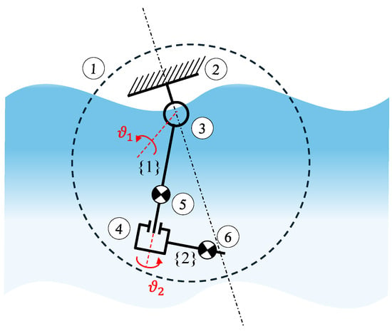
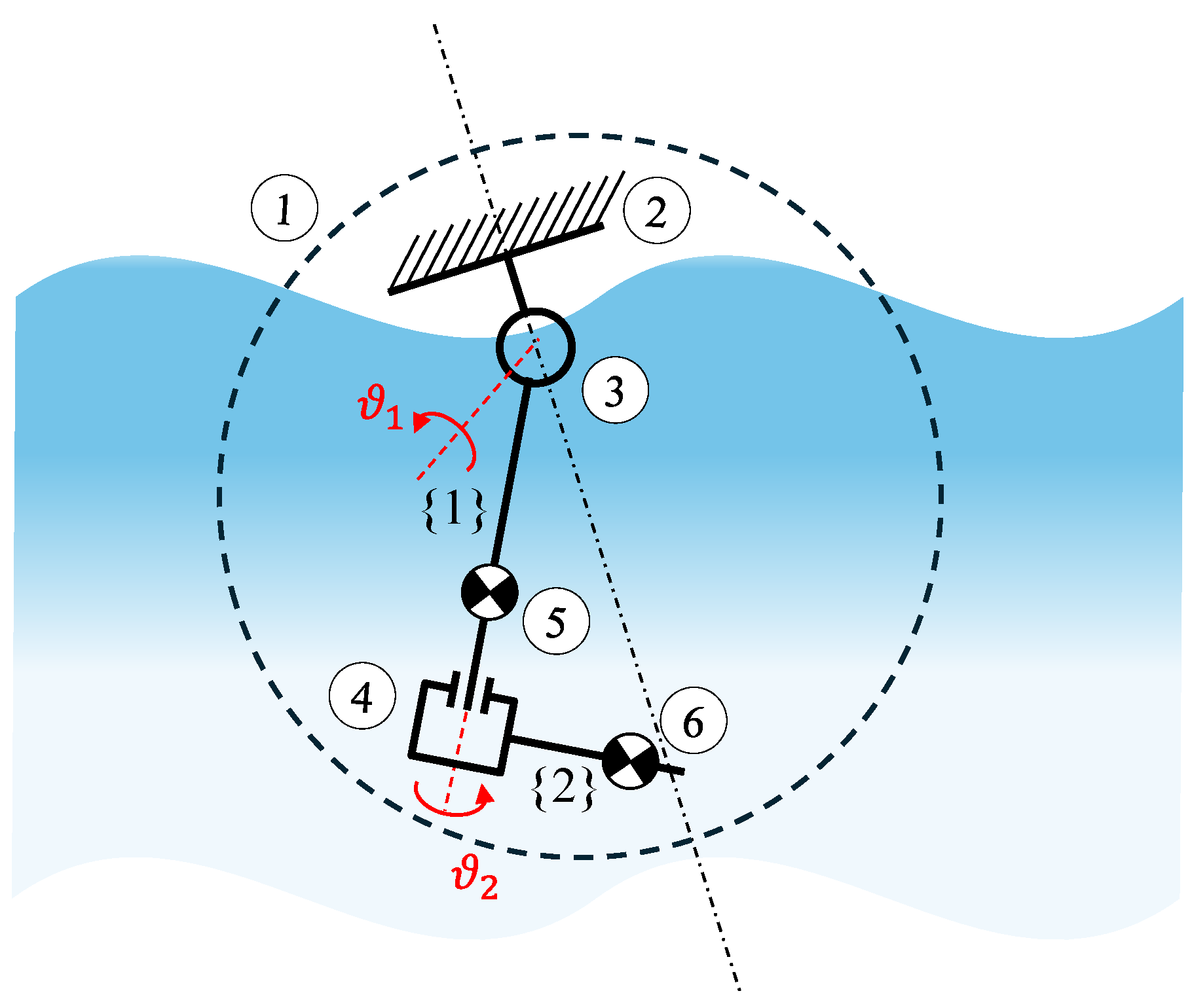
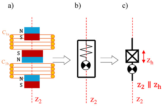
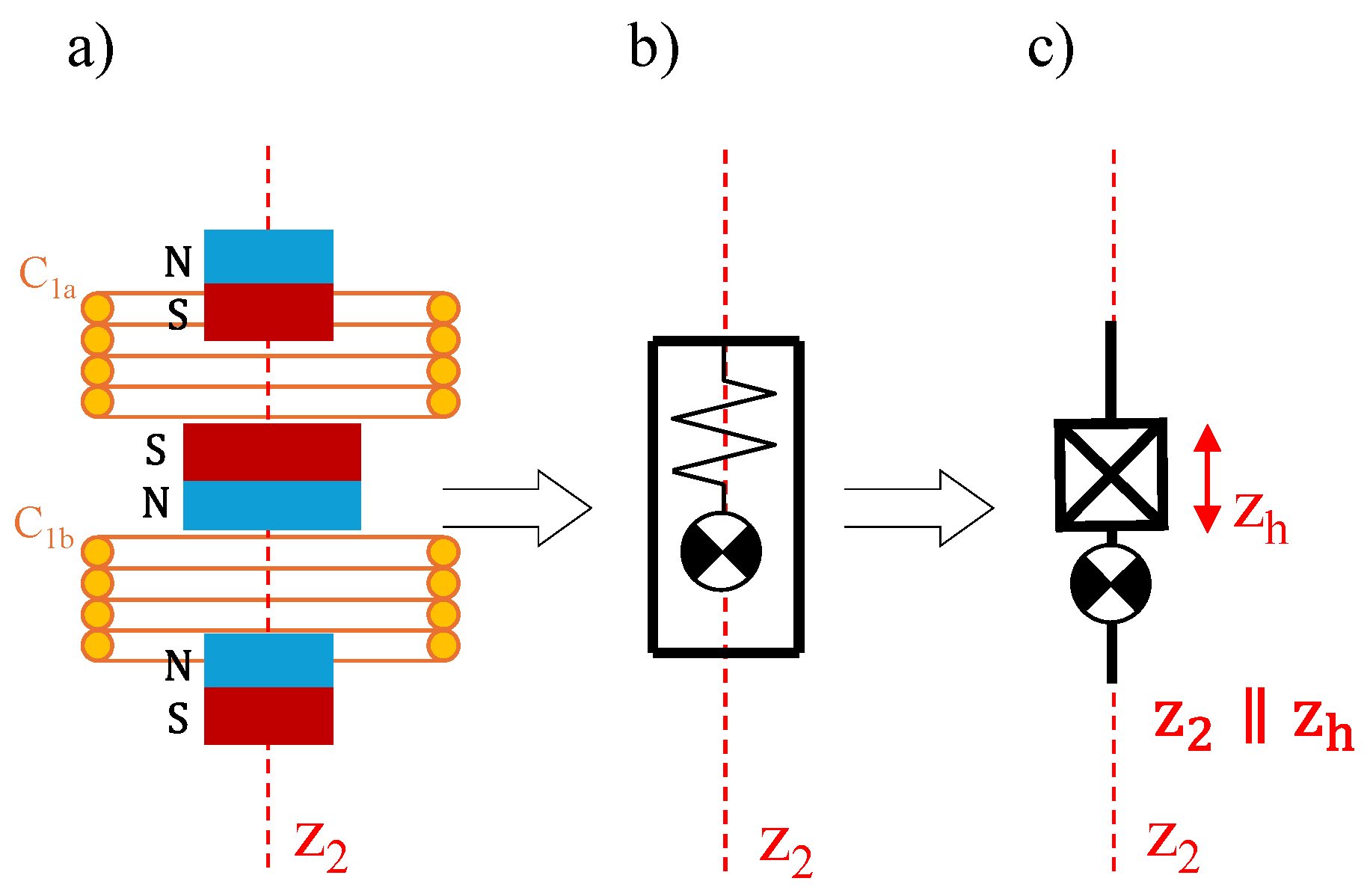
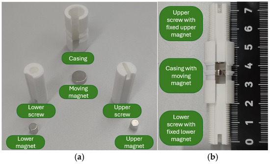
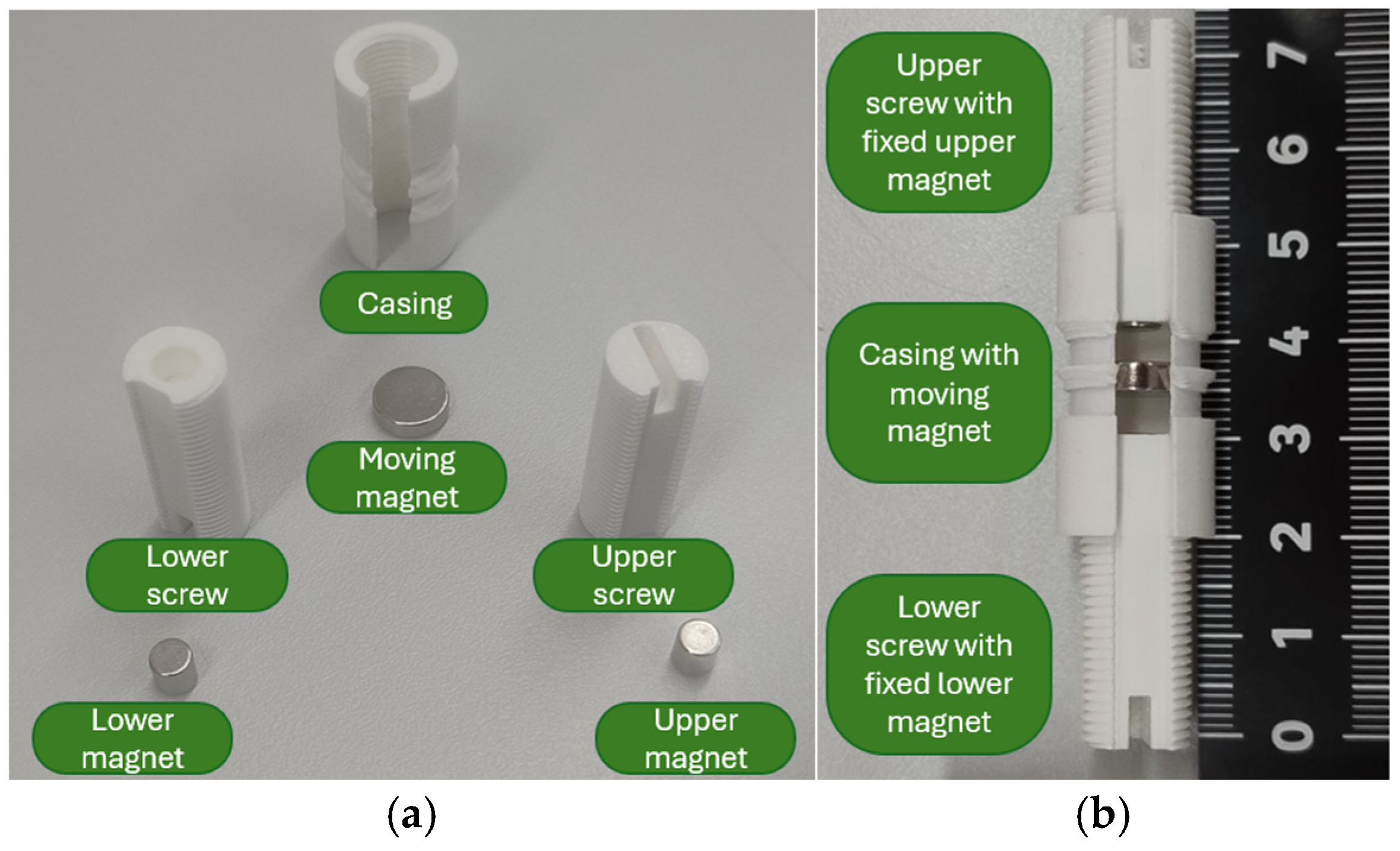
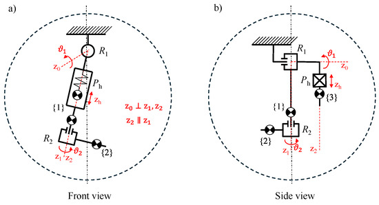
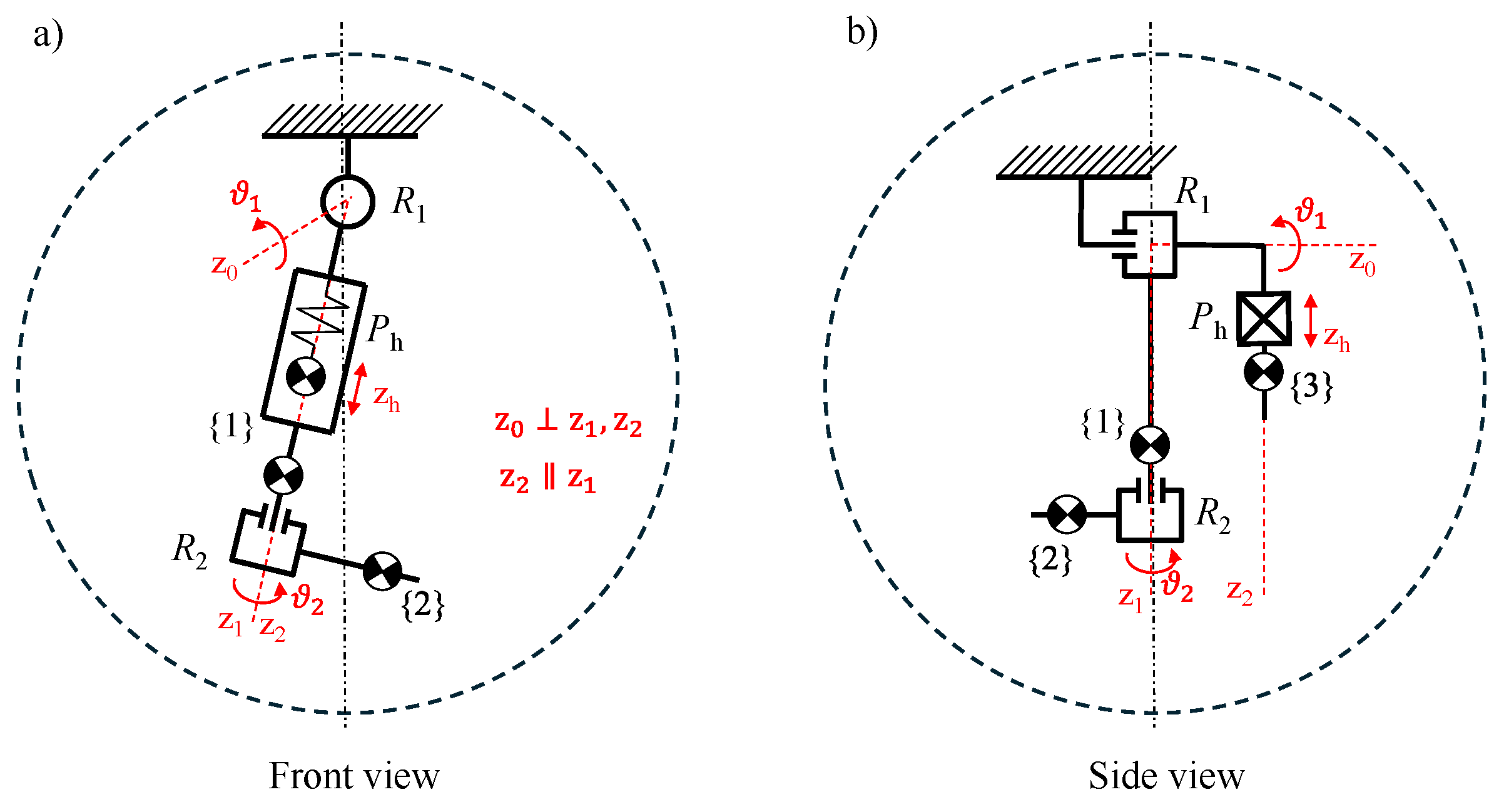
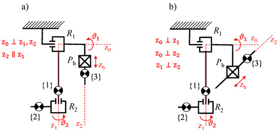
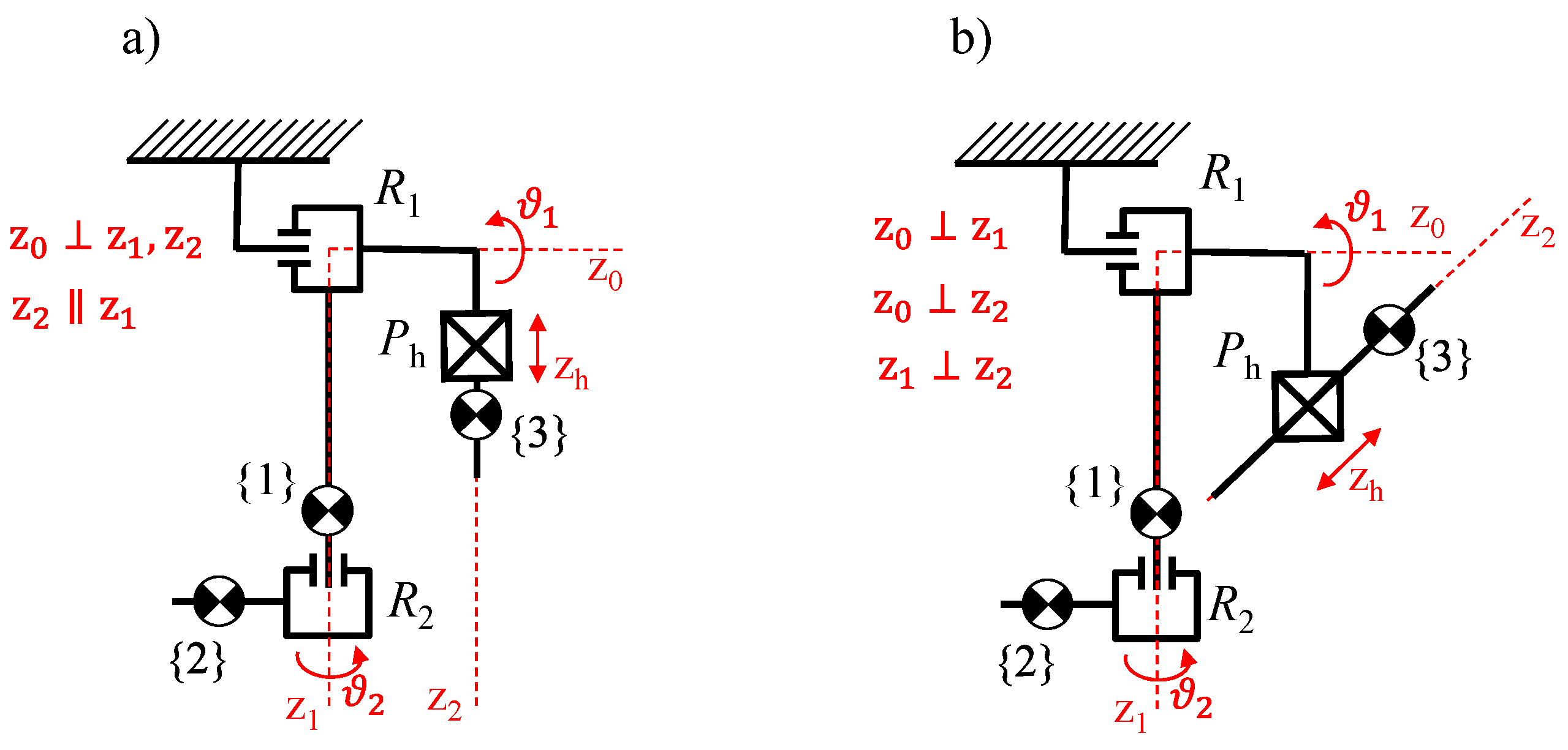
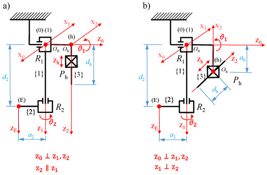
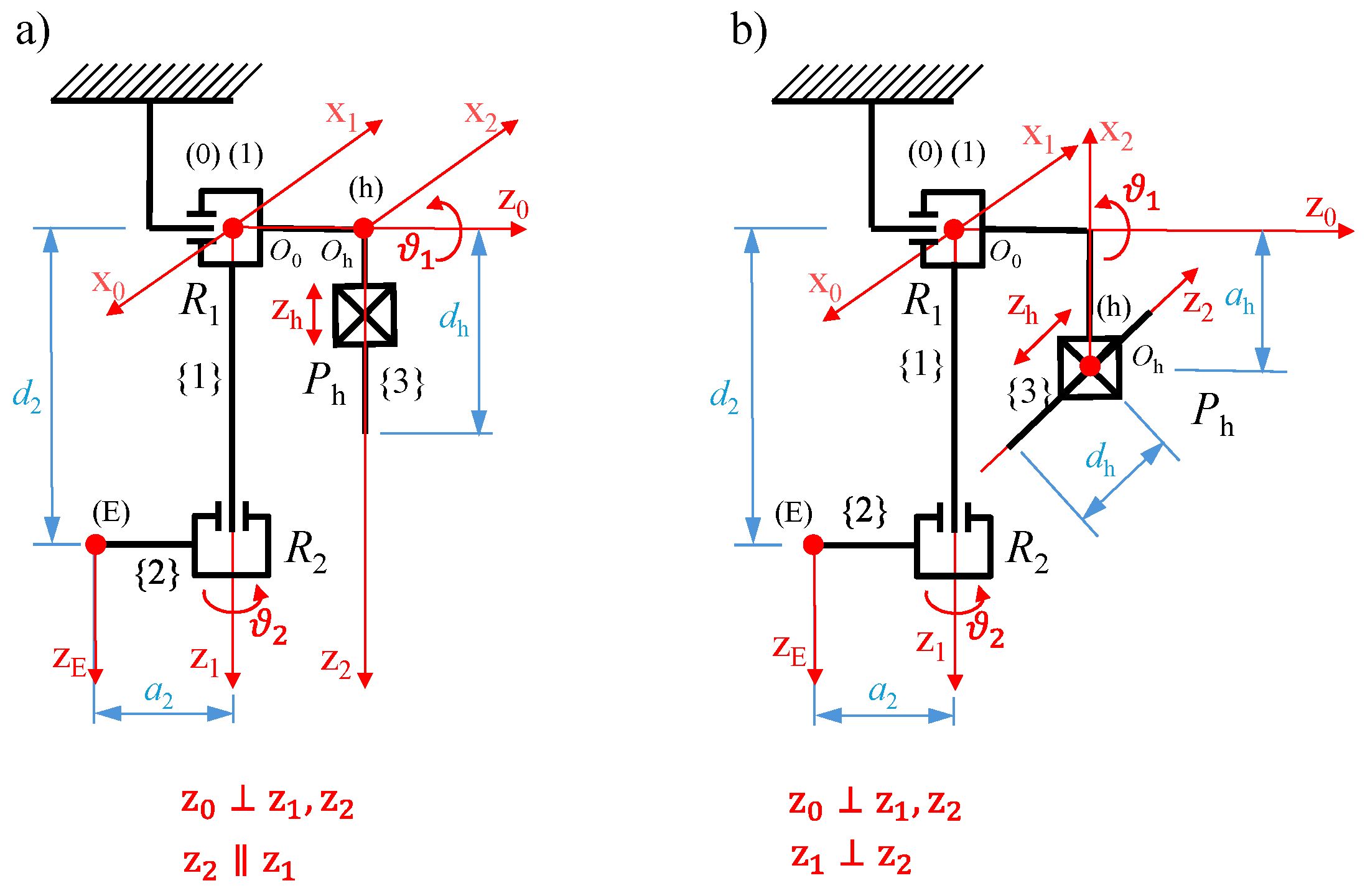
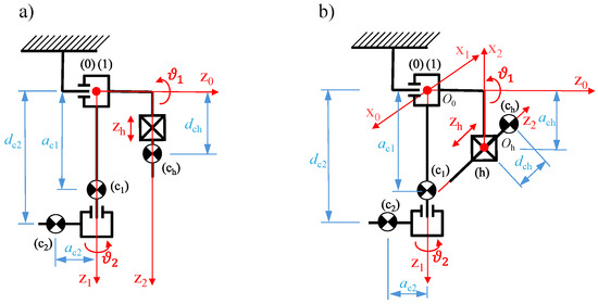
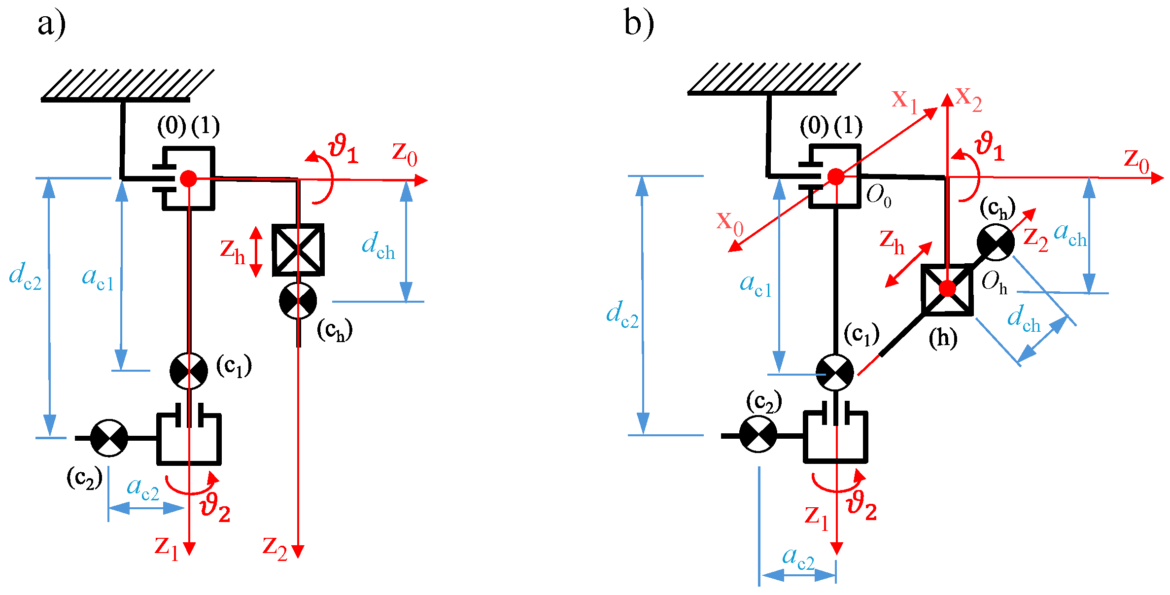
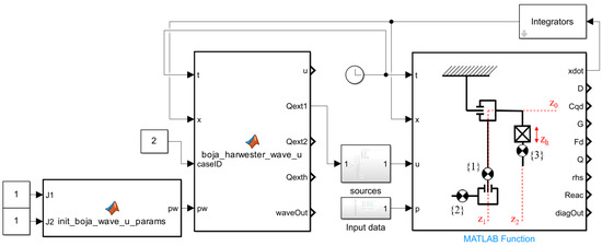
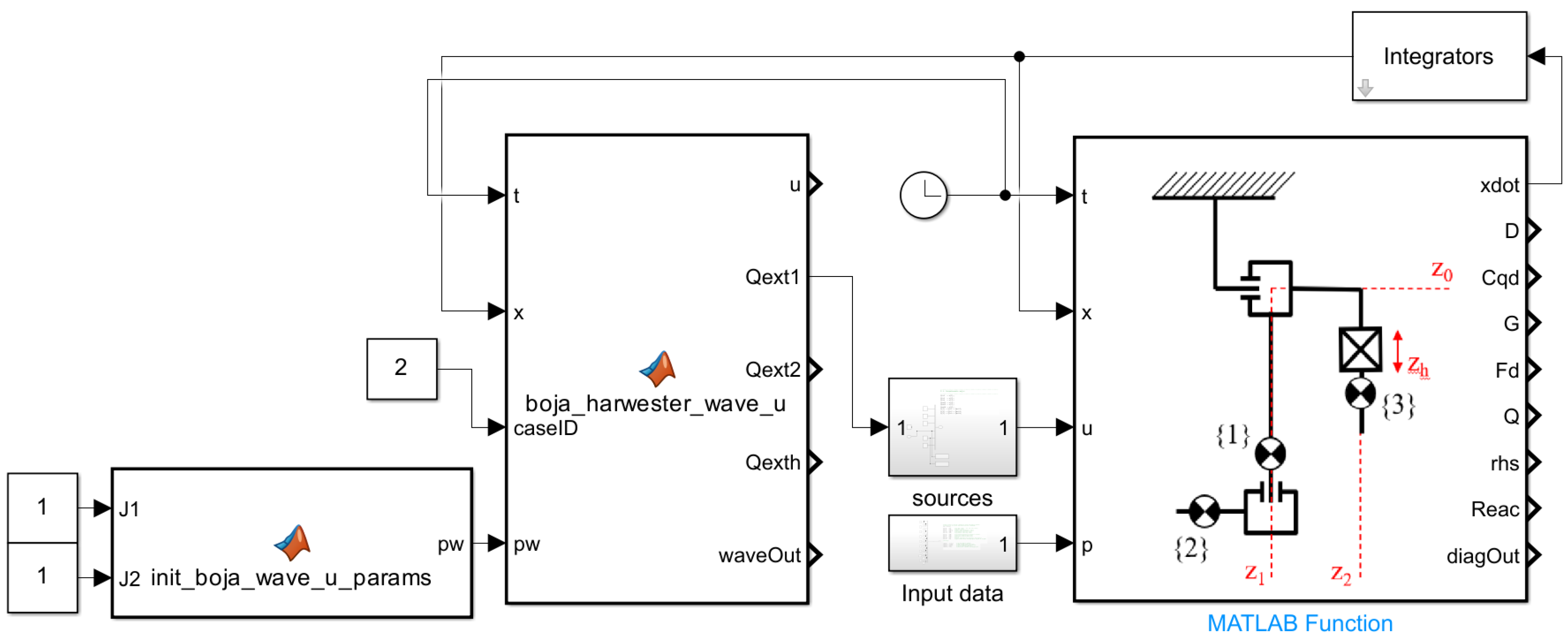
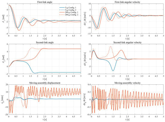
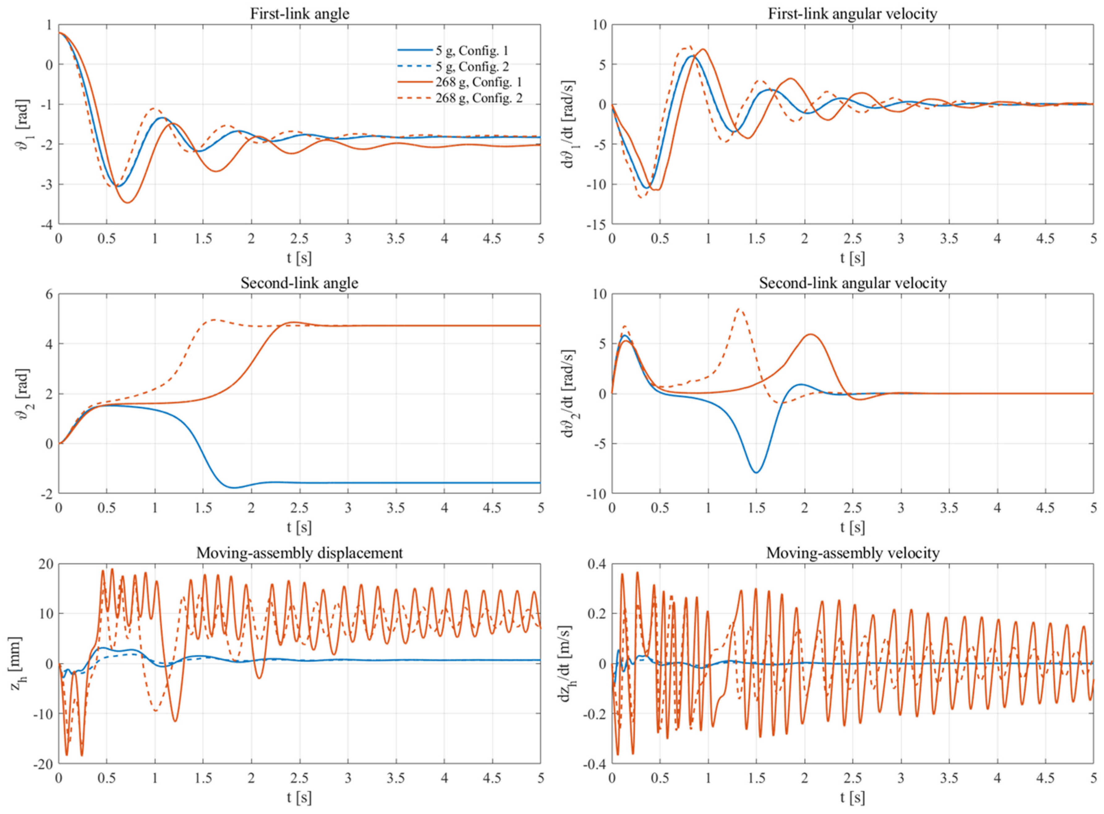
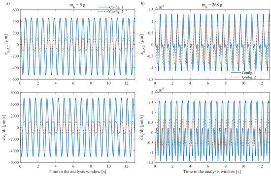
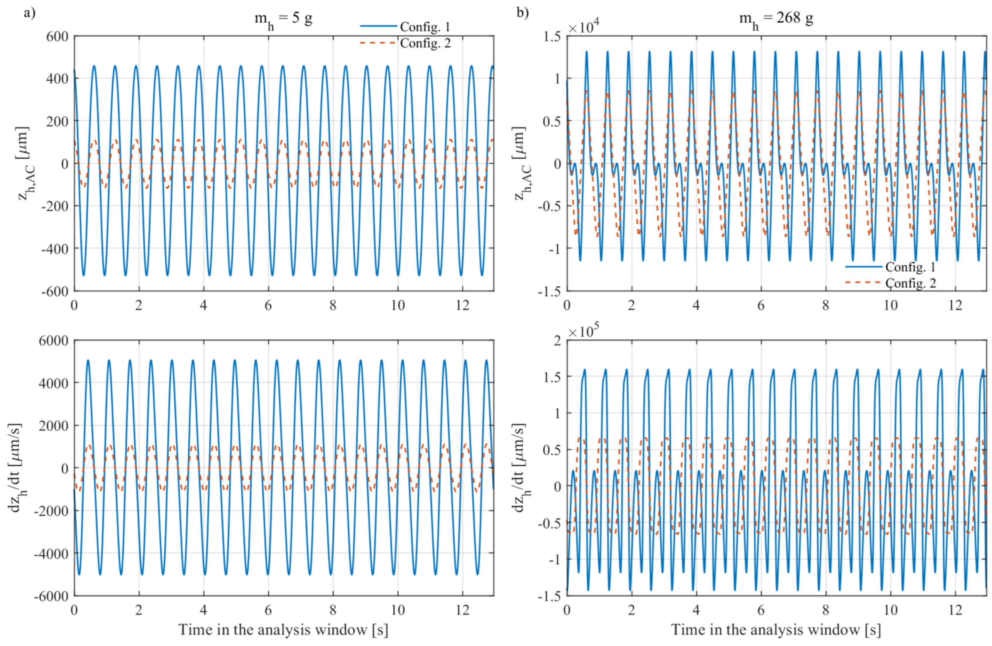
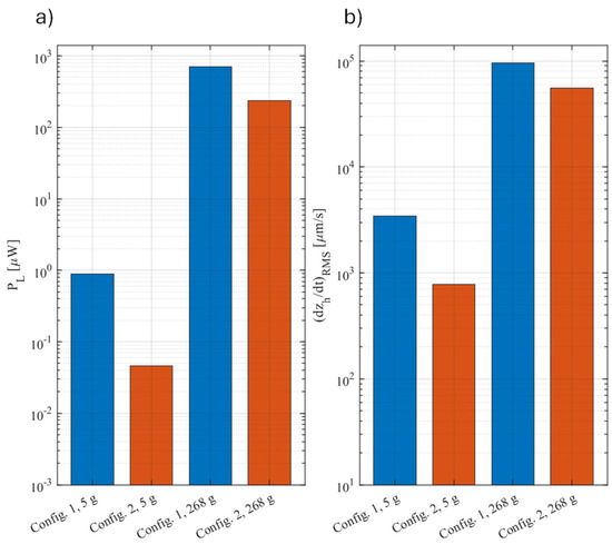
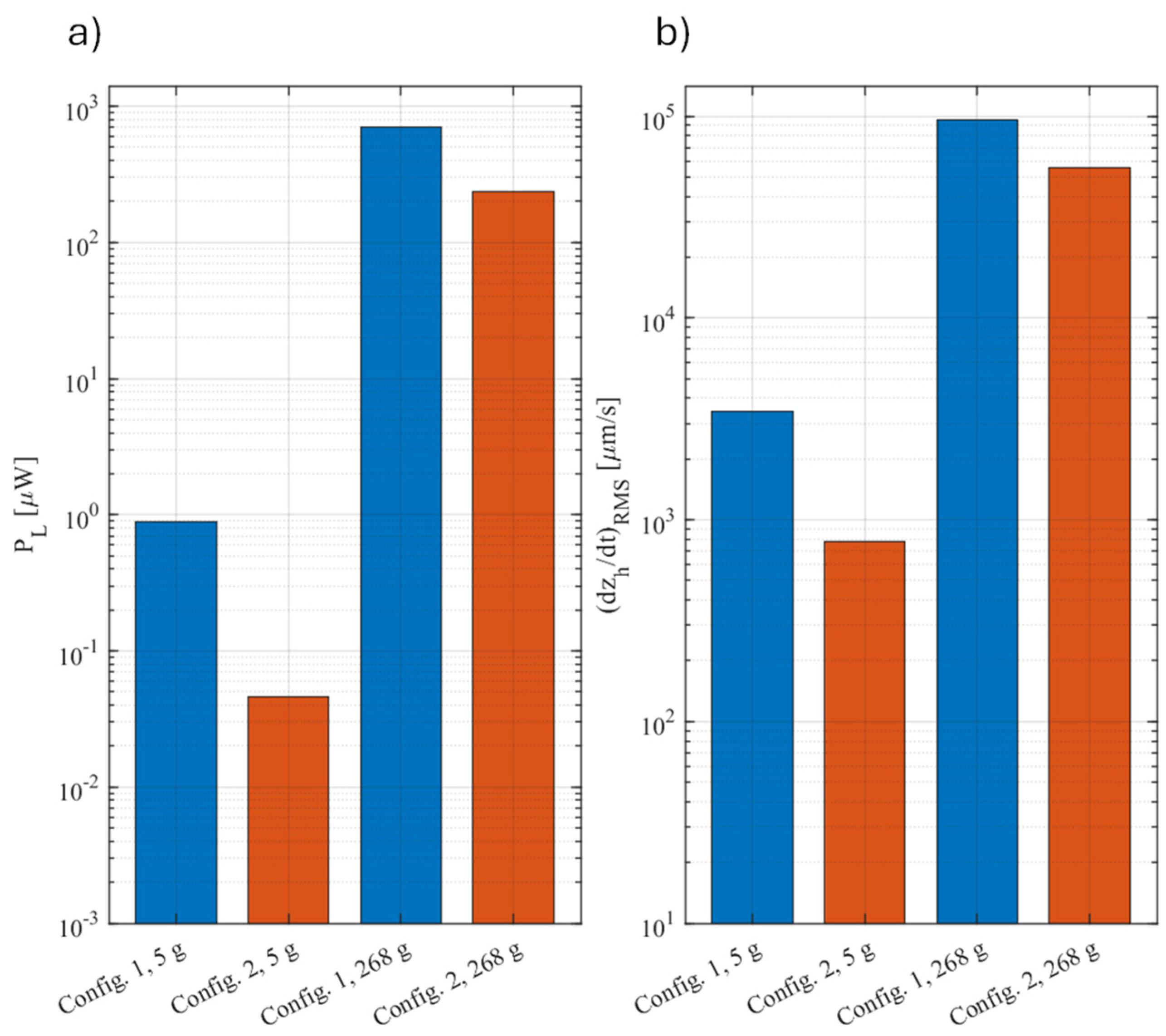
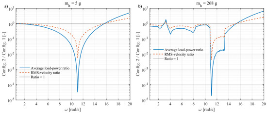
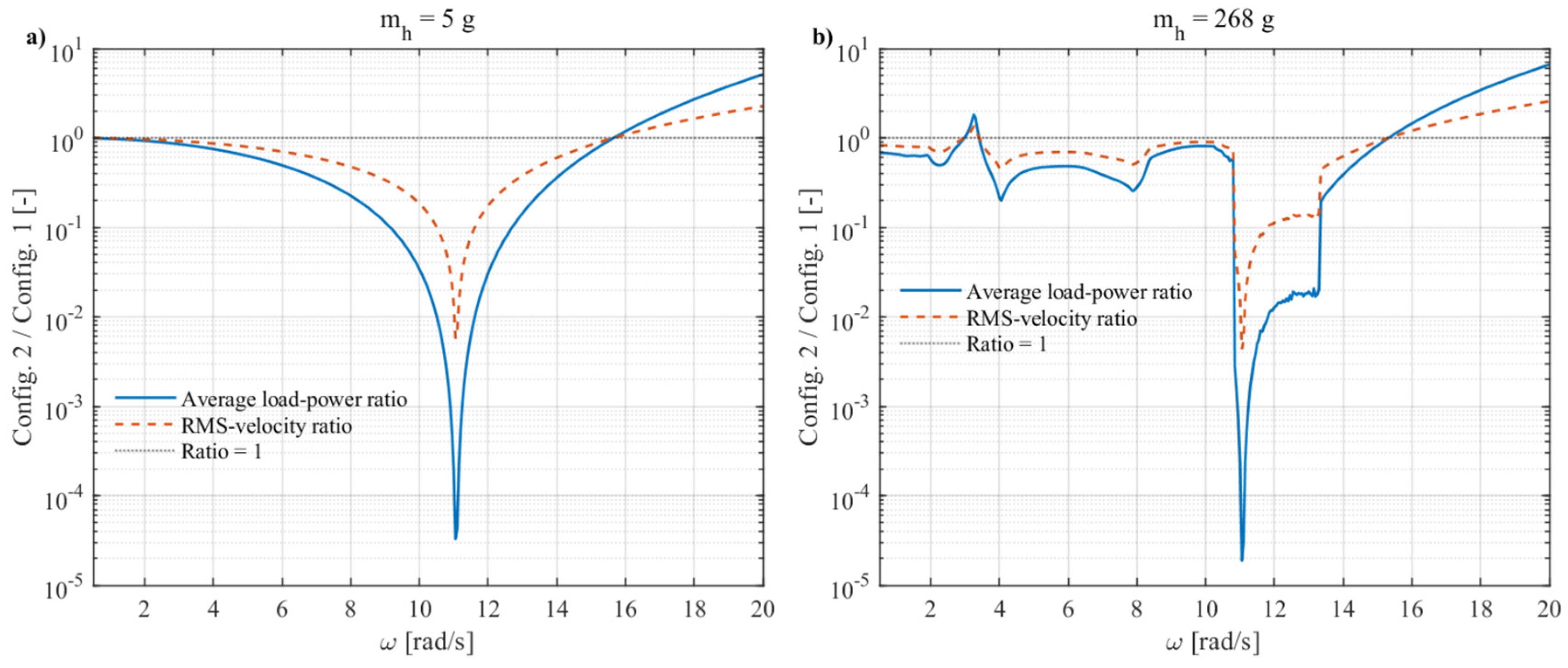
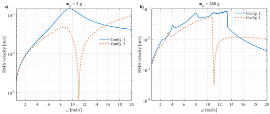
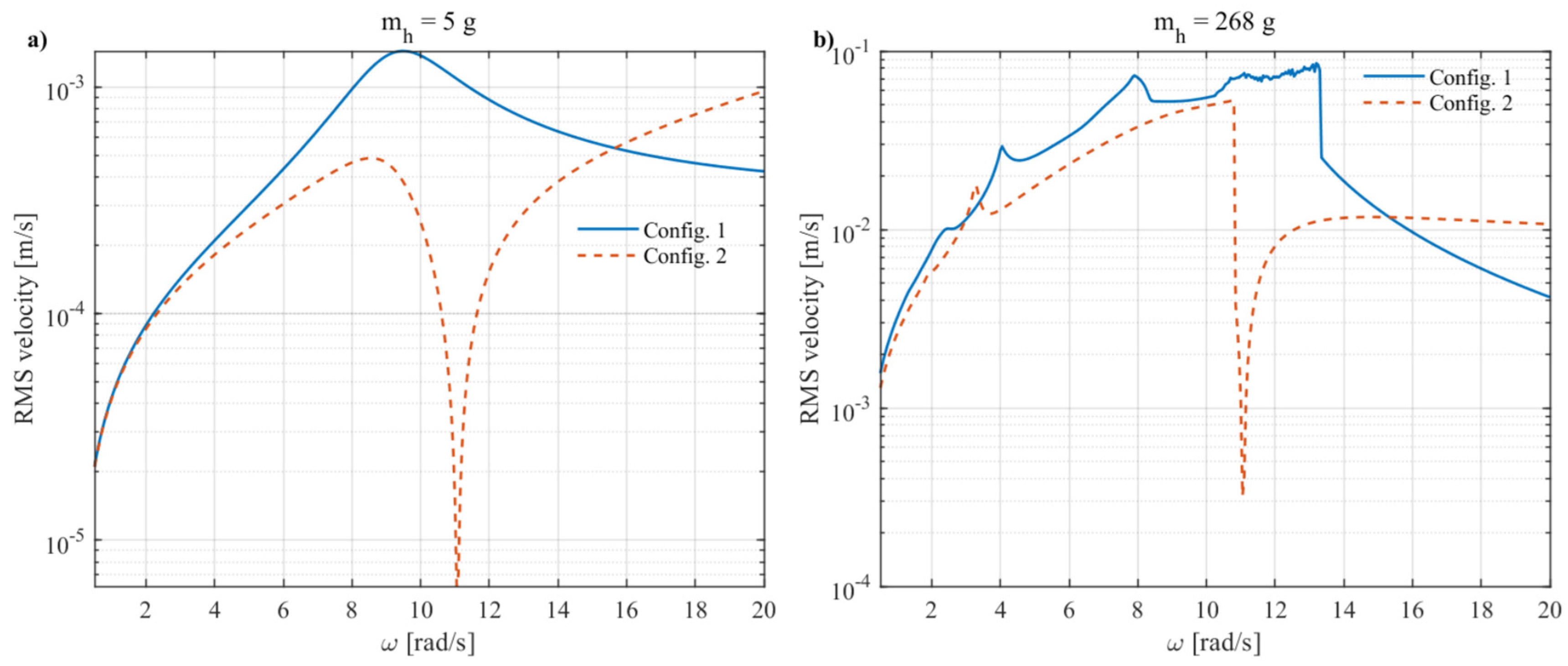
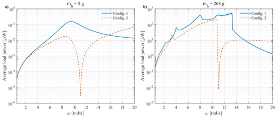
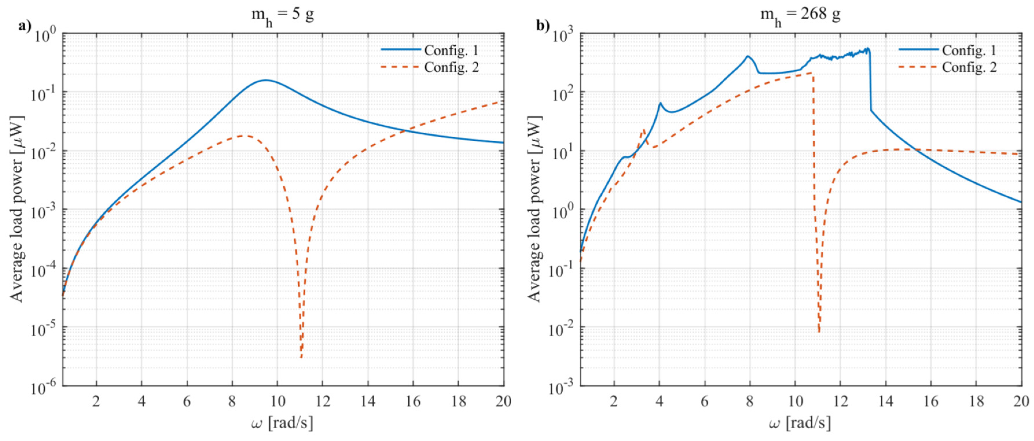
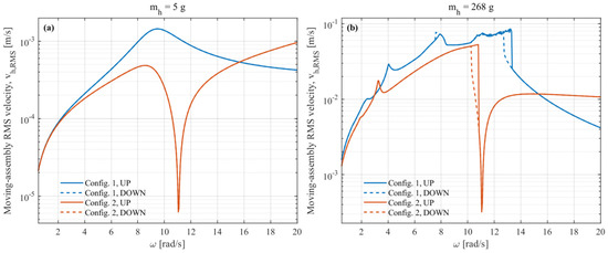
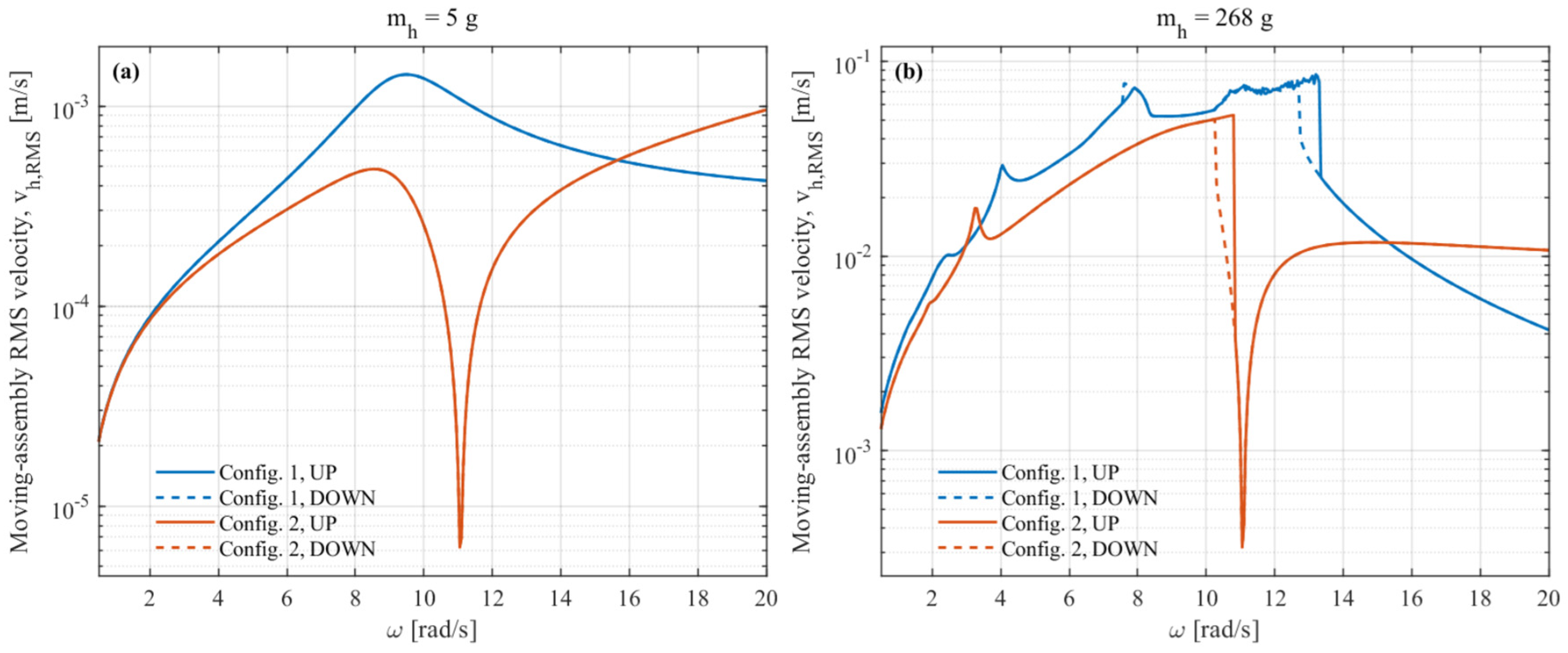
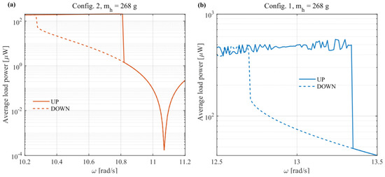
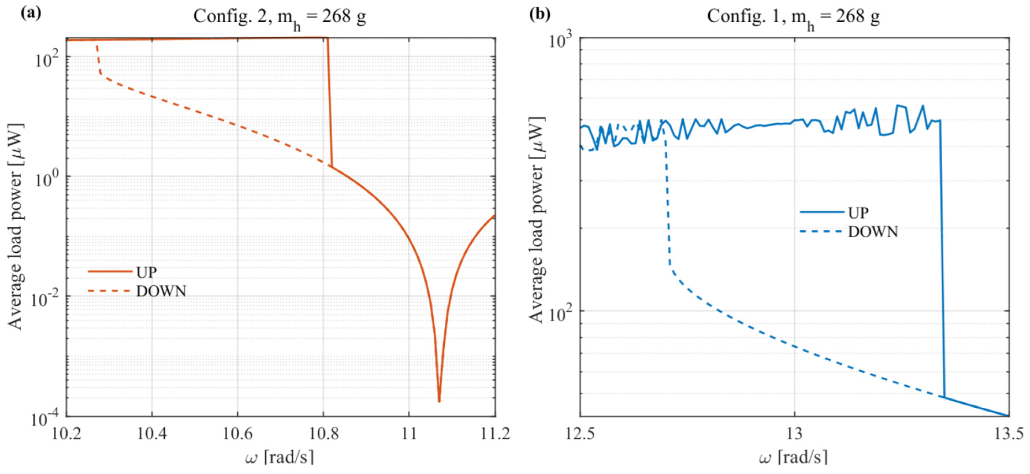

Disclaimer/Publisher’s Note: The statements, opinions and data contained in all publications are solely those of the individual author(s) and contributor(s) and not of MDPI and/or the editor(s). MDPI and/or the editor(s) disclaim responsibility for any injury to people or property resulting from any ideas, methods, instructions or products referred to in the content. |
© 2026 by the authors. Licensee MDPI, Basel, Switzerland. This article is an open access article distributed under the terms and conditions of the Creative Commons Attribution (CC BY) license.