Utility Harmonic Impedance Estimation Based on Isolation Forest and Bernaola Galvan Method

Abstract

Traditional non-invasive harmonic impedance estimation methods often suffer from significant accuracy degradation or even failure under conditions of large background harmonic voltage fluctuations and abrupt changes in harmonic impedance. To address these challenges, a novel estimation method for utility harmonic impedance is proposed. First, a sliding-window-based isolation forest (IF) method is proposed to extract data segments exhibiting a strong correlation between harmonic voltage and current, thereby reducing the adverse impact of background harmonic voltage fluctuations on the impedance estimation results. Then, the Bernaola Galvan (BG) method is proposed to detect abrupt change points in harmonic impedance, and data are grouped accordingly based on the detected change points. Finally, a binary linear regression method is employed to estimate the utility harmonic impedance. The proposed method is validated using both simulation and field data, achieving relative errors below 4% and outperforming conventional methods under complex conditions.

1. Introduction

With the large-scale integration of distributed generation, such as photovoltaic and wind power, the number of harmonic sources in power systems has increased significantly [1,2]. The injected harmonics exhibit new characteristics, including uncertainty, variability, and intermittency, which pose new challenges to the harmonic analysis in modern power systems [3]. To accurately allocate harmonic responsibility and effectively mitigate harmonic pollution, it is essential to evaluate the harmonic emission levels of both the utility side and the consumer side at the point of common coupling (PCC) [4].

Accurate estimation of utility harmonic impedance is a prerequisite for harmonic emission assessment [5]. Existing harmonic impedance estimation methods can be broadly classified into two categories: invasive and non-invasive approaches [6]. Invasive methods estimate the utility harmonic impedance by injecting disturbances or altering the network topology; however, such approaches may adversely affect the normal operation of the power system [7]. Non-invasive methods estimate harmonic impedance without disturbing normal system operation by utilizing natural fluctuations in loads or the system itself, along with measurable parameters [8].

Non-invasive methods include the fluctuation methods [9,10], linear regression methods [11,12,13,14,15,16], independent component analysis methods [17], and independent random vector methods [18]. Owing to their non-invasive nature and negligible impact on system operation, these methods are widely adopted. However, their performance is highly susceptible to background harmonic voltage fluctuations and abrupt changes in harmonic impedance, which may lead to significant estimation errors.

To mitigate the influence of background harmonic voltage fluctuations, a common strategy is to select data segments at the PCC where harmonic voltage and current exhibit strong correlation. The Pearson correlation coefficient is employed in [19] to filter harmonic data, which effectively reduces the impact of background harmonic voltage fluctuations but is sensitive to outliers. The dynamic time warping (DTW) method is used to select data with high waveform similarity, addressing sequence misalignment issues at the expense of increased computational complexity [16]. A time series cluster method is proposed to filter harmonic data based on the cross-correlation principle, but its performance depends heavily on empirically selected thresholds [20].

In addition, variations in system operating conditions, capacitor bank switching, and changes in reactive power compensation schemes may result in abrupt changes in utility harmonic impedance. If such variations are not properly considered, conventional estimation methods may exhibit poor real-time performance and large estimation errors.

Currently, studies addressing abrupt changes in harmonic impedance remain limited. A slope comparison method is proposed in [21], where abrupt changes are identified when the slope exceeds a predefined threshold; however, its performance degrades in scenarios with multiple change points or similar slope characteristics. In [22], minimum norm of impedance difference method is used to segment measured data for detecting impedance variations, but the results are sensitive to background harmonic voltage fluctuations. A DBSCAN clustering algorithm is applied to group data based on harmonic impedance, but it struggles to distinguish cases with small impedance variations and is highly dependent on parameter selection [23].

Based on the above analysis, to mitigate the influence of background harmonic fluctuations, accurately identify the change points in harmonic impedance, and further improve the accuracy of impedance estimation, a novel harmonic impedance estimation method is proposed in this paper. The main contributions of the paper are listed as follows.

• First, a sliding-window-based Isolation Forest (IF) method is proposed to filter harmonic data, thereby extracting data segments with strong correlation between harmonic voltage and current.
• Then, based on the filter data, the Bernaola Galvan (BG) method is proposed to detect the abrupt change points in harmonic impedance.
• Finally, a binary linear regression is applied to estimate the utility harmonic impedance for each data group separately.

The rest of the paper is organized as follows. Section 2 describes the equivalent circuit and the fundamentals for utility harmonic impedance estimation. Section 3 introduces the harmonic data filtering method based on a sliding-window-based IF method. Section 4 presents the BG method to identify the abrupt change points in harmonic impedance. Section 5 verifies the validity of the proposed method using simulation results. Section 6 further discusses the validity of the proposed method using the real power system data. The paper is concluded in Section 7.

2. Fundamental Principle of Harmonic Impedance Estimation

To establish a solid theoretical foundation for the proposed method, this section first reviews the Thevenin equivalent circuit of the power system. By analyzing the mathematical relationship between harmonic voltage and current, we identify the key constraints of traditional regression methods, which justify the necessity of the subsequent data filtering and change-point detection stages.

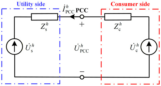
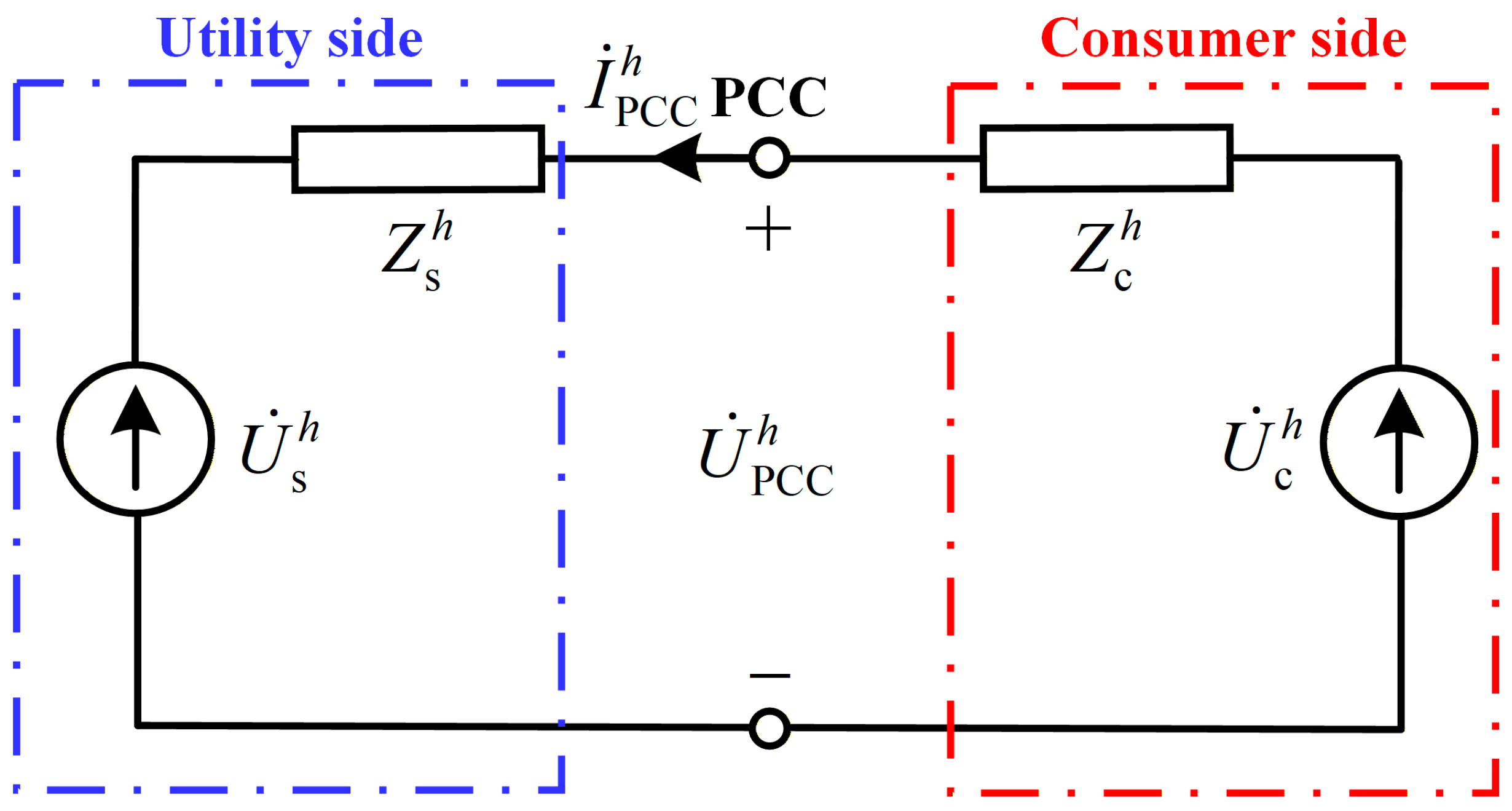
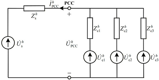
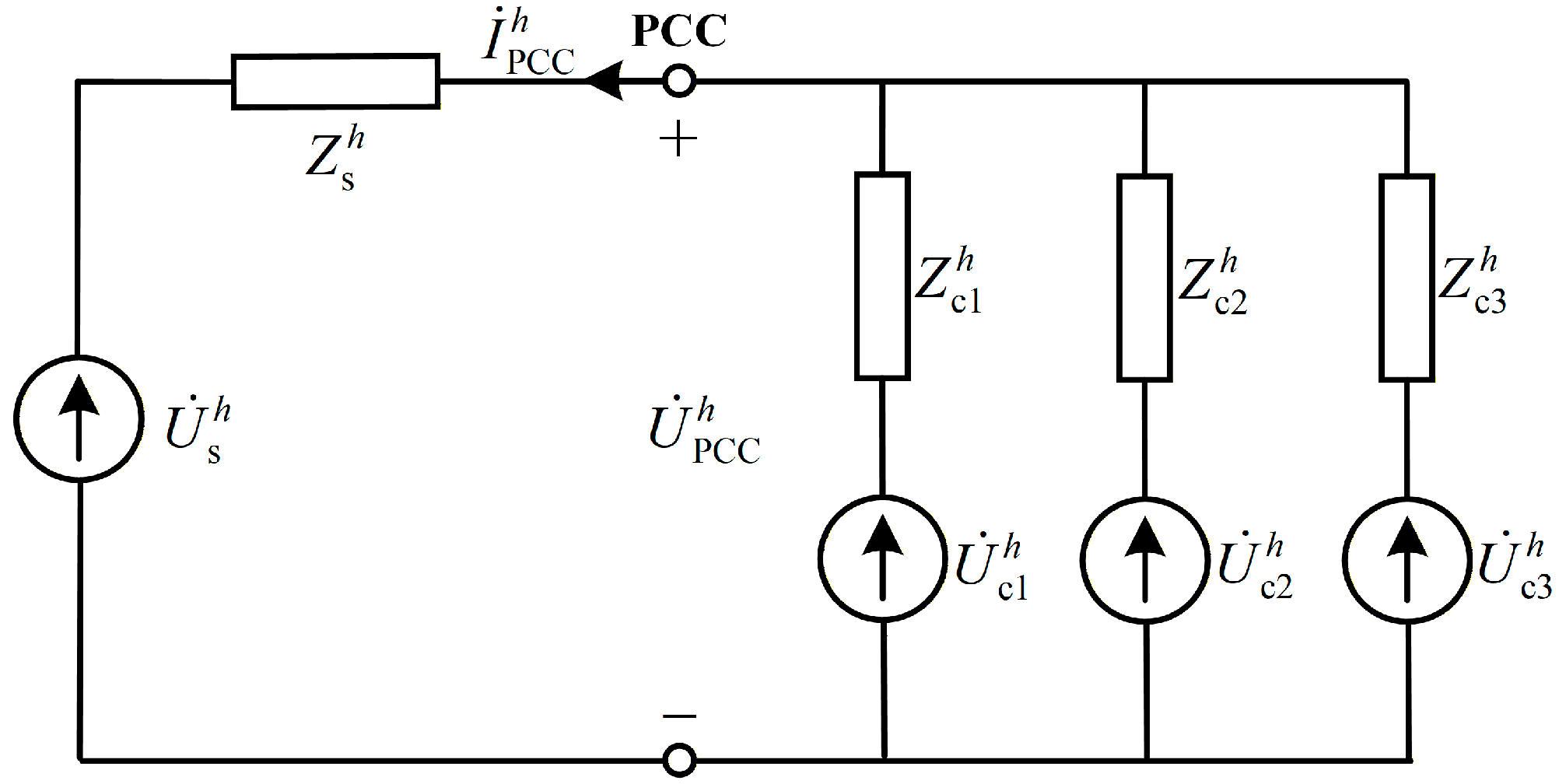
As shown in Figure 1, the Thevenin equivalent circuit is commonly used to estimate the harmonic impedance. By measuring the harmonic voltage and current data at the point of common coupling (PCC), the utility harmonic impedance can be estimated.

Figure 1. Thevenin equivalent circuit for harmonic impedance analysis.

Based on the Thevenin equivalent circuit shown in Figure 1, it can be obtained that [20]

$${\dot{U}}_{\mathrm{PCC}}^h=Z_{\mathrm{s}}^h{\dot{I}}_{\mathrm{PCC}}^h+{\dot{U}}_{\mathrm{s}}^h$$

(1)

where ${\dot{U}}_{\mathrm{PCC}}^h$ and ${\dot{I}}_{\mathrm{PCC}}^h$ are the hth harmonic voltage and current vectors at the PCC; $Z_{\mathrm{s}}^h$ is the hth utility harmonic impedance; ${\dot{U}}_{\mathrm{s}}^h$ is the background harmonic voltage vector.

From (1), over a certain time interval, when the utility harmonic impedance $Z_{\mathrm{s}}^h$ remains constant and the background harmonic voltage ${\dot{U}}_{\mathrm{s}}^h$ are relatively stable, the utility harmonic impedance $Z_{\mathrm{s}}^h$ can be calculated by performing linear regression on the harmonic voltage ${\dot{U}}_{\mathrm{PCC}}^h$ and current ${\dot{I}}_{\mathrm{PCC}}^h$.

At point k, the real and imaginary parts of (1) are separated as

$$U_{\mathrm{PCC}\_\mathrm{x}}^h(k)=Z_{\mathrm{s}\_\mathrm{x}}^h{I}_{\mathrm{PCC}\_\mathrm{x}}^h(k)-Z_{\mathrm{s}\_\mathrm{y}}^h{I}_{\mathrm{PCC}\_\mathrm{y}}^h(k)+U_{\mathrm{s}\_\mathrm{x}}^h$$

(2)

$$U_{\mathrm{PCC}\_\mathrm{y}}^h(k)=Z_{\mathrm{s}\_\mathrm{x}}^h{I}_{\mathrm{PCC}\_\mathrm{y}}^h(k)+Z_{\mathrm{s}\_\mathrm{y}}^h{I}_{\mathrm{PCC}\_\mathrm{x}}^h(k)+U_{\mathrm{s}\_\mathrm{y}}^h$$

(3)

where the subscript x is the real part and the subscript y is the imaginary part.

By performing bivariate linear regression on (2) and (3), the utility harmonic impedance and the background harmonic voltage can be estimated, respectively [13,14]. Over a given time interval, bivariate linear regression is performed on (2) and (3), and the corresponding solution can be expressed as

$$\begin{array}{c}\min f(Z_{\mathrm{s}\_\mathrm{x}}^h,Z_{\mathrm{s}\_\mathrm{y}}^h,U_{\mathrm{s}\_\mathrm{x}}^h)={\displaystyle {\sum }_{k=1}^N|} U_{\mathrm{PCC}\_\mathrm{x}}^h(k)-Z_{\mathrm{s}\_\mathrm{x}}^h\times \\ I_{\mathrm{PCC}\_\mathrm{x}}^h(k)+Z_{\mathrm{s}\_\mathrm{y}}^h{I}_{\mathrm{PCC}\_\mathrm{y}}^h(k)-U_{\mathrm{s}\_\mathrm{x}}^h|\end{array}$$

(4)

$$\begin{array}{c}\min f(Z_{\mathrm{s}\_\mathrm{x}}^h,Z_{\mathrm{s}\_\mathrm{y}}^h,U_{\mathrm{s}\_\mathrm{y}}^h)={\displaystyle {\sum }_{k=1}^N|} U_{\mathrm{PCC}\_\mathrm{y}}^h(k)-Z_{\mathrm{s}\_\mathrm{x}}^h\times \\ I_{\mathrm{PCC}\_\mathrm{y}}^h(k)-Z_{\mathrm{s}\_\mathrm{y}}^h{I}_{\mathrm{PCC}\_\mathrm{x}}^h(k)-U_{\mathrm{s}\_\mathrm{y}}^h|\end{array}$$

(5)

Solve (4) and (5) respectively [24], and the solutions are

$${[{\widehat{Z}}_{\mathrm{s}\_\mathrm{x}}^h {\widehat{Z}}_{\mathrm{s}\_\mathrm{y}}^h {\widehat{U}}_{\mathrm{s}\_\mathrm{x}}^h]}^{\mathrm{T}}={({\mathit{A}}^{\mathrm{T}}\mathit{A})}^{-1}{\mathit{A}}^{\mathrm{T}}\mathit{Y}$$

(6)

$${[{\widehat{Z}}_{\mathrm{s}\_\mathrm{x}1}^h {\widehat{Z}}_{\mathrm{s}\_\mathrm{y}1}^h {\widehat{U}}_{\mathrm{s}\_\mathrm{y}}^h]}^{\mathrm{T}}={({\mathit{A}}_1^{\mathrm{T}}{\mathit{A}}_1)}^{-1}{\mathit{A}}_1^{\mathrm{T}}{\mathit{Y}}_1$$

(7)

where A is the regression matrix; A^T is the transpose of A; A⁻¹ is the inverse of A.

. $$\left\{\mathit{Y}=\left[\begin{array}{c}{U}_{\mathrm{PCC}\_\mathrm{x}}^h(1)\\ U_{\mathrm{PCC}\_\mathrm{x}}^h(2)\\ ⋮\\ U_{\mathrm{PCC}\_\mathrm{x}}^h(N)\end{array}\right]\right.,{\mathit{Y}}_1=\left[\begin{array}{c}{U}_{\mathrm{PCC}\_\mathrm{y}}^h(1)\\ U_{\mathrm{PCC}\_\mathrm{y}}^h(2)\\ ⋮\\ U_{\mathrm{PCC}\_\mathrm{y}}^h(N)\end{array}\right]$$

(8)

$$\left\{\begin{array}{l}\mathit{A}=\left[\begin{array}{ccc}{I}_{\mathrm{PCC}\_\mathrm{x}}^h(1)& -I_{\mathrm{PCC}\_\mathrm{y}}^h(1)& 1\\ I_{\mathrm{PCC}\_\mathrm{x}}^h(2)& -I_{\mathrm{PCC}\_\mathrm{y}}^h(2)& 1\\ \begin{array}{l}⋮\\ I_{\mathrm{PCC}\_\mathrm{x}}^h(N)\end{array}& \begin{array}{l}⋮\\ -I_{\mathrm{PCC}\_\mathrm{y}}^h(N)\end{array}& \begin{array}{l}⋮\\ 1\end{array}\end{array}\right]\\ {\mathit{A}}_1=\left[\begin{array}{ccc}{I}_{\mathrm{PCC}\_\mathrm{y}}^h(1)& I_{\mathrm{PCC}\_\mathrm{x}}^h(1)& 1\\ I_{\mathrm{PCC}\_\mathrm{y}}^h(2)& I_{\mathrm{PCC}\_\mathrm{x}}^h(2)& 1\\ \begin{array}{l}⋮\\ I_{\mathrm{PCC}\_\mathrm{y}}^h(N)\end{array}& \begin{array}{l}⋮\\ I_{\mathrm{PCC}\_\mathrm{x}}^h(N)\end{array}& \begin{array}{l}⋮\\ 1\end{array}\end{array}\right]\end{array}\right.$$

(9)

The utility harmonic impedance estimated from (6) and (7) is

$$\left[\begin{array}{l}{Z}_{\mathrm{s}\_\mathrm{real}}^h\\ Z_{\mathrm{s}\_\mathrm{imag}}^h\end{array}\right]=\left[\begin{array}{l}({\widehat{Z}}_{\mathrm{s}\_\mathrm{x}}^h+{\widehat{Z}}_{\mathrm{s}\_\mathrm{x}1}^h)/2\\ ({\widehat{Z}}_{\mathrm{s}\_\mathrm{y}}^h+{\widehat{Z}}_{\mathrm{s}\_\mathrm{y}1}^h)/2\end{array}\right]$$

(10)

However, under practical operating conditions, variations in system operating modes, switching of reactive power compensation devices, and the inherent variability of renewable energy sources can lead to changes in both the background harmonic voltage ${\dot{U}}_{\mathrm{s}}^h$ and the utility harmonic impedance $Z_{\mathrm{s}}^h$, making the regression methods unsuitable for utility harmonic impedance estimation.

To address the above issues, a novel method is proposed that: (1) filters harmonic data with significant background harmonic voltage fluctuations; (2) detects abrupt change points in harmonic impedance.

3. The Sliding-Window-Based Isolation Forest Method

To improve the accuracy of harmonic impedance estimation under background harmonic voltage fluctuations, a data filtering method based on sliding-window IF is proposed. The method aims to identify data segments with relatively stable background harmonic voltage and remove abnormal data points within these segments, thereby enhancing the reliability of subsequent regression analysis.

3.1. Sliding Window Construction

This subsection details the construction of sliding windows, which serves as the temporal basis for localized data processing.

As shown in Figure 2. Let the sliding time window have a length of L and a step size of s; then, the mth sliding window is defined as follows

$$w_m=\{k|m\le k\le m+L-1\}$$

(11)

where m is the starting index of the sliding window; L is the window length.

Figure 2. Sliding process.

The selection of L and s involves a trade-off between statistical stability and temporal resolution. A larger window length L provides more data samples within each window, which improves the robustness of the subsequent regression analysis and reduces the influence of measurement noise. However, an excessively large L may smooth out local variations and reduce the sensitivity to abrupt changes. Conversely, a smaller step size $s$ increases the overlap between adjacent windows, allowing finer tracking of time-varying characteristics, but at the cost of increased computational burden. Therefore, L and s are selected to ensure sufficient data samples for reliable estimation while maintaining adequate resolution for detecting impedance variations.

In this study, the window length and step size are set to L = 20 and s = 5, respectively, for both simulation and field data analysis. These values are chosen to ensure sufficient data samples for reliable regression while maintaining adequate sensitivity to impedance variations. Sensitivity analysis indicates that moderate variations in L and s do not significantly affect the estimation accuracy.

The entire data sequence is divided into multiple sliding time windows. This time window limits the temporal scope of correlation detection, preventing changes in the global data distribution from affecting the correlation assessment results.

3.2. Linear Correlation Analysis

After constructing sliding windows to segment the harmonic data, a linear correlation analysis method is adopted to test the linear correlation of the regression results of (4) and (5), thereby selecting the data segments suitable for harmonic impedance calculation.

According to the principles of mathematical statistics, linear correlation can be evaluated using the F-statistic. Based on the result of (6), over a sample interval of length N, the linearity F₁ of the regression in (4) is calculated as

$$F_1={\displaystyle \frac{S_{\mathrm{R}}/2}{S_{\mathrm{E}}/(N-3)}}$$

(12)

$$\begin{array}{c}{S}_{\mathrm{R}}={\displaystyle {\sum }_{k=m}^{m+L-1}|} {\widehat{Z}}_{\mathrm{s}\_\mathrm{x}}{I}_{\mathrm{PCC}\_\mathrm{x}}(k)-{\widehat{Z}}_{\mathrm{s}\_\mathrm{y}}{I}_{\mathrm{PCC}\_\mathrm{y}}(k)+\\ {\widehat{U}}_{\mathrm{s}\_\mathrm{x}}-{\displaystyle \frac{1}{N}}{\displaystyle {\sum }_{k=m}^{m+L-1}[U_{\mathrm{PCC}\_\mathrm{x}}(k)]}{|}^2\end{array}$$

(13)

$$\begin{array}{c}{S}_{\mathrm{E}}={\displaystyle {\sum }_{k=m}^{m+L-1}|} U_{\mathrm{PCC}\_\mathrm{x}}(k)-{\widehat{Z}}_{\mathrm{s}\_\mathrm{x}}{I}_{\mathrm{PCC}\_\mathrm{x}}(k)+\\ {\widehat{Z}}_{\mathrm{s}\_\mathrm{y}}{I}_{\mathrm{PCC}\_\mathrm{y}}(k)-{\widehat{U}}_{\mathrm{s}\_\mathrm{x}}{|}^2\end{array}$$

(14)

Meanwhile, based on the result of (7), the regression linearity of (5) is calculated, denoted as F₂. Larger values of F₁ and F₂ indicate more significant linearity and more accurate and reliable estimation results, whereas smaller values imply poorer linearity and larger estimation errors. The overall linearity of the bivariate linear regression method is defined as

$$F=F_1+F_2$$

(15)

Therefore, a linearity threshold F_t can be set, and data segments satisfying F > F_t are selected for harmonic impedance estimation, thereby improving the accuracy of the estimation results. In this work, the threshold is empirically set to F_t = 50, which provides a good balance between data quality and data availability in both simulation and field scenarios.

It should be noted that the method is not highly sensitive to the exact value of F_t; similar performance can be achieved within a reasonable range of threshold values. This enhances the robustness and practical applicability of the proposed approach.

3.3. Isolation Forest Method

Building upon the segment-level filtering, this subsection employs the IF algorithm to refine the dataset further by removing individual outliers.

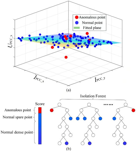
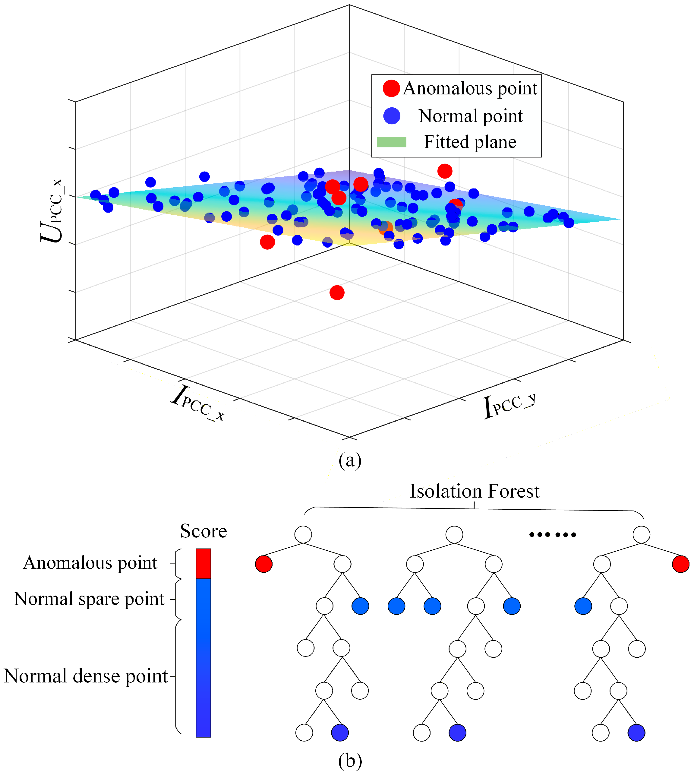
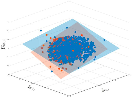
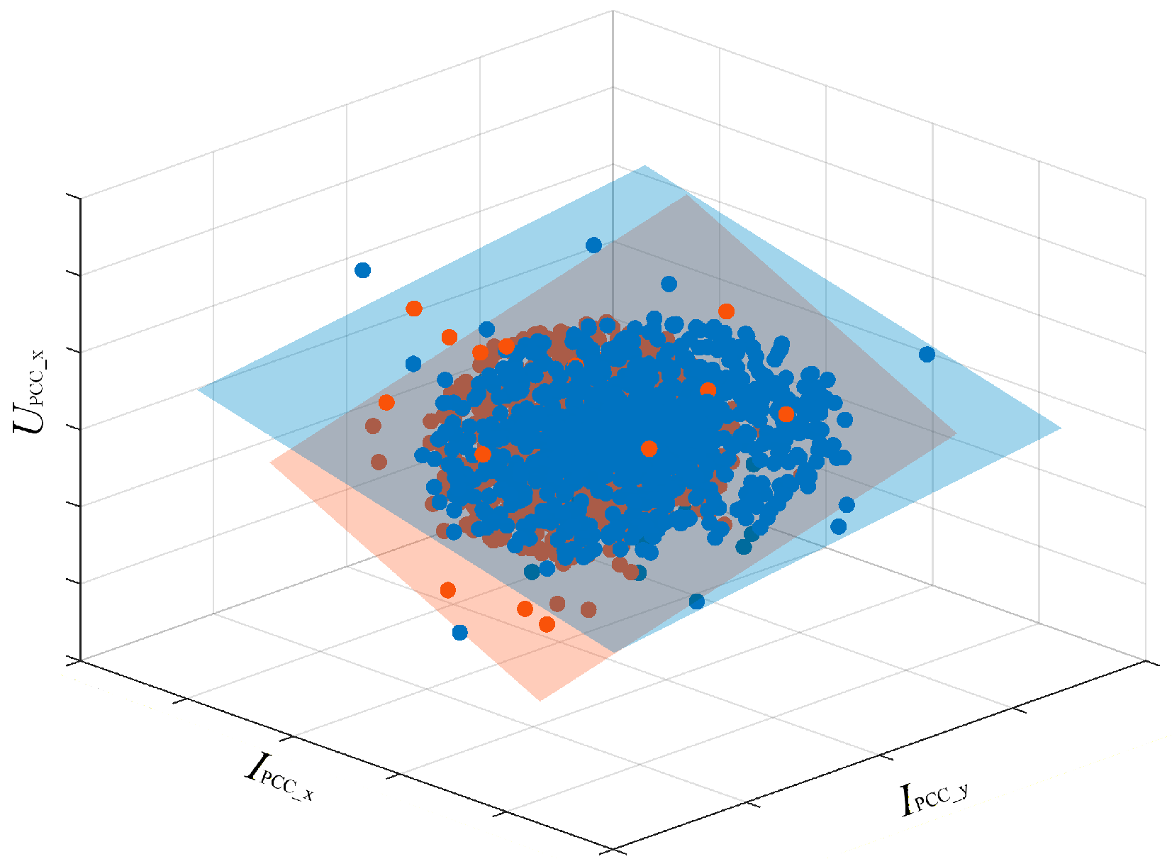
After F-statistic-based filtering, the obtained harmonic data exhibit strong linear correlation, indicating that the background harmonic voltage remains relatively stable within the selected data segments. From (2), when U_{PCC_x}, I_{PCC_x}, and −I_{PCC_y} are taken as the x-, y-, and z-axes, respectively, the filtered data points should approximately lie on a plane, as illustrated in Figure 3a.

Figure 3. Harmonic data outlier removal process. (a) 3D scatter plot of harmonic data. (b) IF anomaly value filtering.

Although the retained segments exhibit strong overall correlation, abnormal data points may still exist due to measurement noise and system disturbances. Since the F-statistic mainly evaluates the overall correlation of a data segment and is not effective in detecting individual outliers, the IF method is further employed to perform point-wise anomaly detection. As shown in Figure 3b, the identified anomalous points are removed, thereby improving the reliability and accuracy of the subsequent impedance estimation.

In this paper, the number of trees in the IF method is defined as 100. The model is trained independently within each sliding window rather than using a pre-trained global model. This design allows the method to adapt to local data characteristics and improves its effectiveness in handling time-varying operating conditions and non-stationary harmonic behavior.

Since (2) and (3) are based on the same filtering principle, (2) is taken as an example for illustration. First, a feature vector is constructed.

$$\mathit{x}(k)=[U_{\mathrm{PCC}\_\mathrm{x}}^h(k),I_{\mathrm{PCC}\_\mathrm{x}}^h(k),-I_{\mathrm{PCC}\_\mathrm{y}}^h(k)]$$

(16)

For each sample x(k), a random tree is constructed by

(1)

randomly selecting a feature q

(2)

randomly choosing a split value p within the range of that feature

The partitioning continues until the sample is isolated or a predefined depth is reached.

The anomaly score is determined based on the path length from the root node to the terminating node.

Let h(x_k) denote the path length of sample x_k in a single tree. The average path length over T trees is given by

$$E(h({\mathit{x}}_k))={\displaystyle \frac{1}{T}}{\displaystyle \sum _{k=1}^T{h}_k({\mathit{x}}_k)}$$

(17)

The anomaly score is defined as

$$s(x_k,L)=2^{-{\displaystyle \frac{E(h({\mathit{x}}_k))}{c(L)}}}$$

(18)

where c(L) is the normalization factor

$$c(L)=2H(L-1)-{\displaystyle \frac{2(L-1)}{L}}$$

(19)

and H(L) is the harmonic number.

A sample is considered anomalous if

$$s({\mathit{x}}_k)>\tau$$

(20)

where τ is a predefined threshold. In this work, τ is determined based on the distribution of anomaly scores within each window, ensuring adaptive and data-driven anomaly detection.

Although abrupt impedance changes may exhibit transient anomaly-like characteristics, the proposed method does not remove such critical events. This is because the IF method operates on statistically consistent segments and primarily removes isolated outliers, while impedance changes manifest as persistent patterns over multiple samples and can still be reliably captured by the subsequent BG-based detection with the aid of overlapping sliding windows.

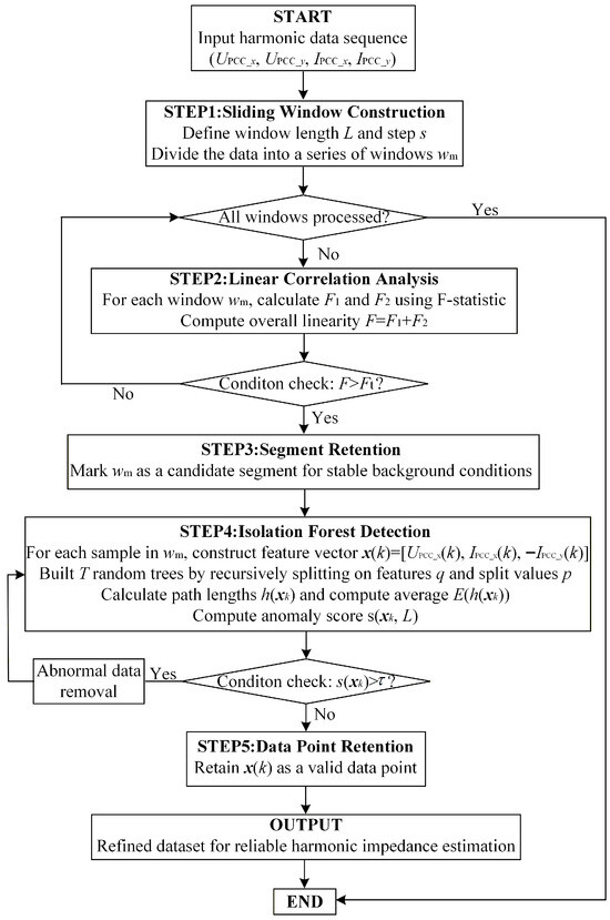
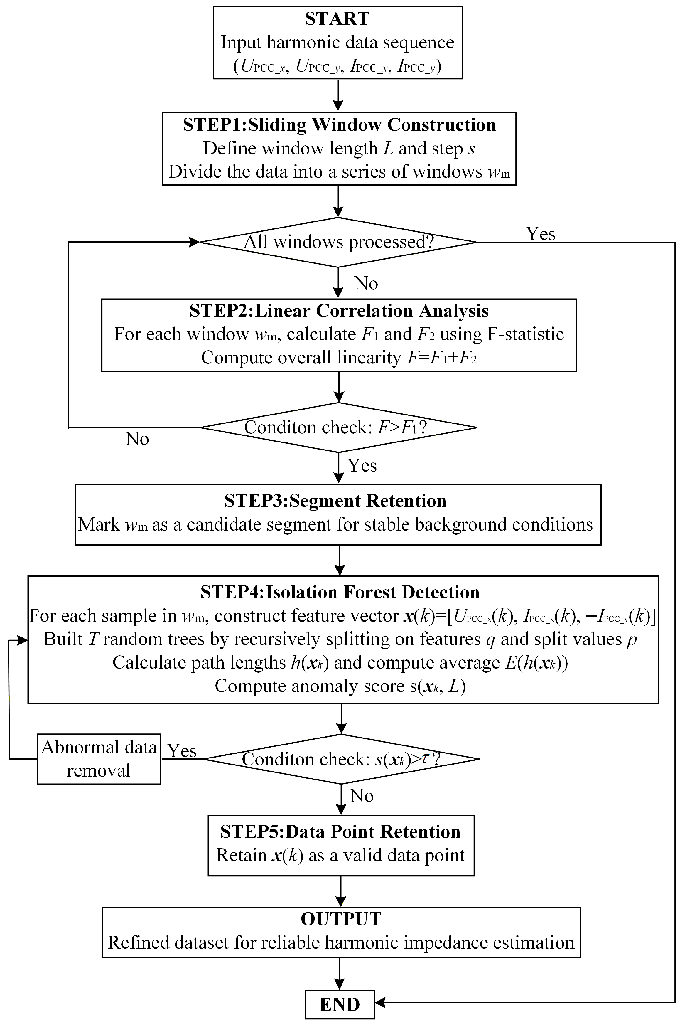
The overall flowchart of the proposed harmonic data filtering method is shown in Figure 4. The procedure consists of two main stages. First, the F-statistic-based filtering is employed to identify data segments with strong linear correlation, ensuring that the background harmonic voltage remains relatively stable within the selected segments. Then, the IF algorithm is applied to perform point-wise anomaly detection within the retained segments, removing abnormal data points caused by measurement noise or system disturbances. Through this two-stage filtering process, the harmonic dataset is refined to retain only reliable samples, which provides a solid foundation for accurate impedance estimation in the subsequent analysis.

Figure 4. Flowchart of the proposed harmonic data filtering method.

4. Bernaola Galvan Method

A prerequisite for harmonic impedance estimation using the bivariate linear regression method is that the utility harmonic impedance remains constant. However, in practical power system operation, the utility harmonic impedance may vary due to changes in operating conditions, load variations, or switching of reactive power compensation devices.

As shown in Figure 5, when the utility harmonic impedance changes, the harmonic data may lie on multiple planes. In this case, using the entire dataset to estimate the harmonic impedance can result in significant errors. Therefore, it is necessary to analyze the issue of abrupt changes in harmonic impedance.

Figure 5. Scatter plot with different colored data points fitted to different planes.

Since the background harmonic voltage of the filtered data is relatively stable, the harmonic impedance can be approximately estimated using the two-point method based on (2).

$$Z_{\mathrm{s}}(k)={\displaystyle \frac{{\dot{U}}_{\mathrm{PCC}}^h(k)-{\dot{U}}_{\mathrm{PCC}}^h(k-1)}{{\dot{I}}_{\mathrm{PCC}}^h(k)-{\dot{I}}_{\mathrm{PCC}}^h(k-1)}}$$

(21)

Express the harmonic voltage and current vectors in terms of their magnitude and phase angle.

$$\left\{\begin{array}{l}{\dot{U}}_{\mathrm{PCC}}^h(k)=U_{\mathrm{PCC}}^h(k)\angle {\alpha }_k\\ {\dot{I}}_{\mathrm{PCC}}^h(k)=I_{\mathrm{PCC}}^h(k)\angle {\beta }_k\end{array}\right.$$

(22)

Then, the magnitude of the utility harmonic impedance is

$$\begin{array}{l}\left|Z_{\mathrm{s}}^h(k)\right|={\displaystyle \frac{\Delta {\dot{U}}_{\mathrm{PCC}}^h}{\Delta {\dot{I}}_{\mathrm{PCC}}^h}}={\displaystyle \frac{\left|{\dot{U}}_{\mathrm{PCC}}^h(k)-{\dot{U}}_{\mathrm{PCC}}^h(k-1)\right|}{\left|{\dot{I}}_{\mathrm{PCC}}^h(k)-{\dot{I}}_{\mathrm{PCC}}^h(k-1)\right|}}=\\ {\displaystyle \frac{\sqrt{{(U_{\mathrm{PCC}}^h(k))}^2+{(U_{\mathrm{PCC}}^h(k-1))}^2-2U_{\mathrm{PCC}}^h(k)U_{\mathrm{PCC}}^h(k-1)\cos ({\alpha }_k-{\alpha }_{k-1})}}{\sqrt{{(I_{\mathrm{PCC}}^h(k))}^2+{(I_{\mathrm{PCC}}^h(k-1))}^2-2I_{\mathrm{PCC}}^h(k)I_{\mathrm{PCC}}^h(k-1)\cos ({\beta }_k-{\beta }_{k-1})}}}\end{array}$$

(23)

From (23), when the current variation is very small ($\Delta {\dot{I}}_{\mathrm{PCC}}^h\to 0$), the denominator approaches zero, which may lead to abnormally large impedance values and introduce significant numerical errors. Such instability can degrade the reliability of the subsequent impedance change detection.

To enhance the robustness of the impedance sequence, a combined window-averaging and threshold-based strategy is proposed. Specifically, a current variation threshold $\epsilon$ is first defined. When the current variation between two adjacent samples satisfies

$$\left|\Delta {\dot{I}}_{\mathrm{PCC}}^h\right|<\epsilon$$

(24)

The corresponding impedance estimate is considered unreliable and is therefore not directly calculated using the two-point difference method. Instead, a sliding window with length H is introduced, within which the voltage and current data are averaged to obtain a more stable estimate of the impedance variation. If the current variation within the window still does not exceed the threshold, the corresponding data point is discarded to prevent abnormal values from affecting the subsequent analysis.

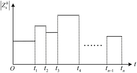
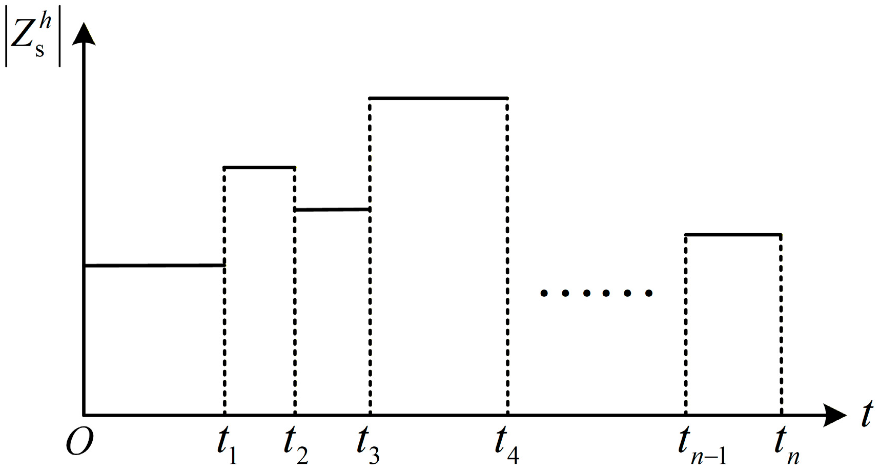
The harmonic impedance remains relatively stable over a period of time and only experiences an abrupt change at specific moments [20]. This behavior can be modeled as shown in Figure 6.

Figure 6. Utility impedance variation model.

The BG method is proposed to detect the abrupt change points in harmonic impedance.

The core idea of the BG method is to segment a sequence such that the statistical properties within each segment are as stable as possible, while significant differences exist between consecutive segments.

Let the approximate harmonic impedance magnitude sequence calculated from (23) be denoted as X.

$$\mathit{X}=\{x_1,x_2,\cdots ,x_n\}$$

(25)

A potential change point c (1 < c < n) is first considered to divide the sequence into two segments

$${\mathit{X}}_{\mathit{L}}=\{x_1,\cdots ,x_c\},{\mathit{X}}_{\mathit{R}}=\{x_{c+1},\cdots ,x_n\}$$

(26)

For each segment, the mean ${\mu }_L$, ${\mu }_R$ and variance ${\sigma }_L^2$, ${\sigma }_R^2$ are calculated

$${\mu }_L={\displaystyle \frac{1}{c}}{\displaystyle {\displaystyle \sum _{i=1}^c}{x}_i},{\mu }_R={\displaystyle \frac{1}{n-c}}{\displaystyle {\displaystyle \sum _{i=c+1}^n}{x}_i}$$

(27)

$${\sigma }_L^2={\displaystyle \frac{1}{c-1}}{\displaystyle {\displaystyle \sum _{i=1}^c}{(x_i-{\mu }_L)}^2, }{\sigma }_R^2={\displaystyle \frac{1}{n-c-1}}{\displaystyle {\displaystyle \sum _{i=c+1}^n}{(x_i-{\mu }_R)}^2}$$

(28)

The standardized mean difference D(c) is then computed to quantify the statistical contrast between the two segments

$$D(c)={\displaystyle \frac{\left|{\mu }_L-{\mu }_R\right|}{\sqrt{\frac{{\sigma }_L^2}{c}+\frac{{\sigma }_R^2}{n-c}}}}$$

(29)

If the maximum value D(c*) exceeds a predefined significance threshold, the point c* is considered a change point. In this study, the statistical significance of the change point is evaluated by calculating the confidence probability, denoted as P(D(c*)). The point c* is considered a change point. To capture all potential changes in the sequence, the BG method recursively applies this procedure to each segment until all sub-segments exhibit relatively stable statistical properties (P(D(c*)) < 0.95) or the segment length falls below a minimum threshold (L_min = 100).

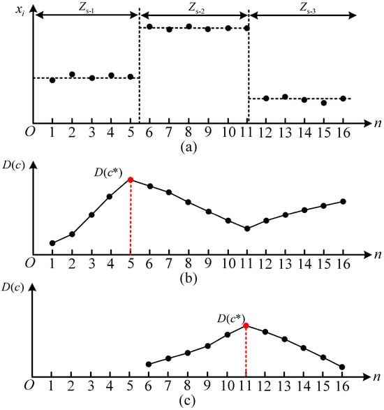
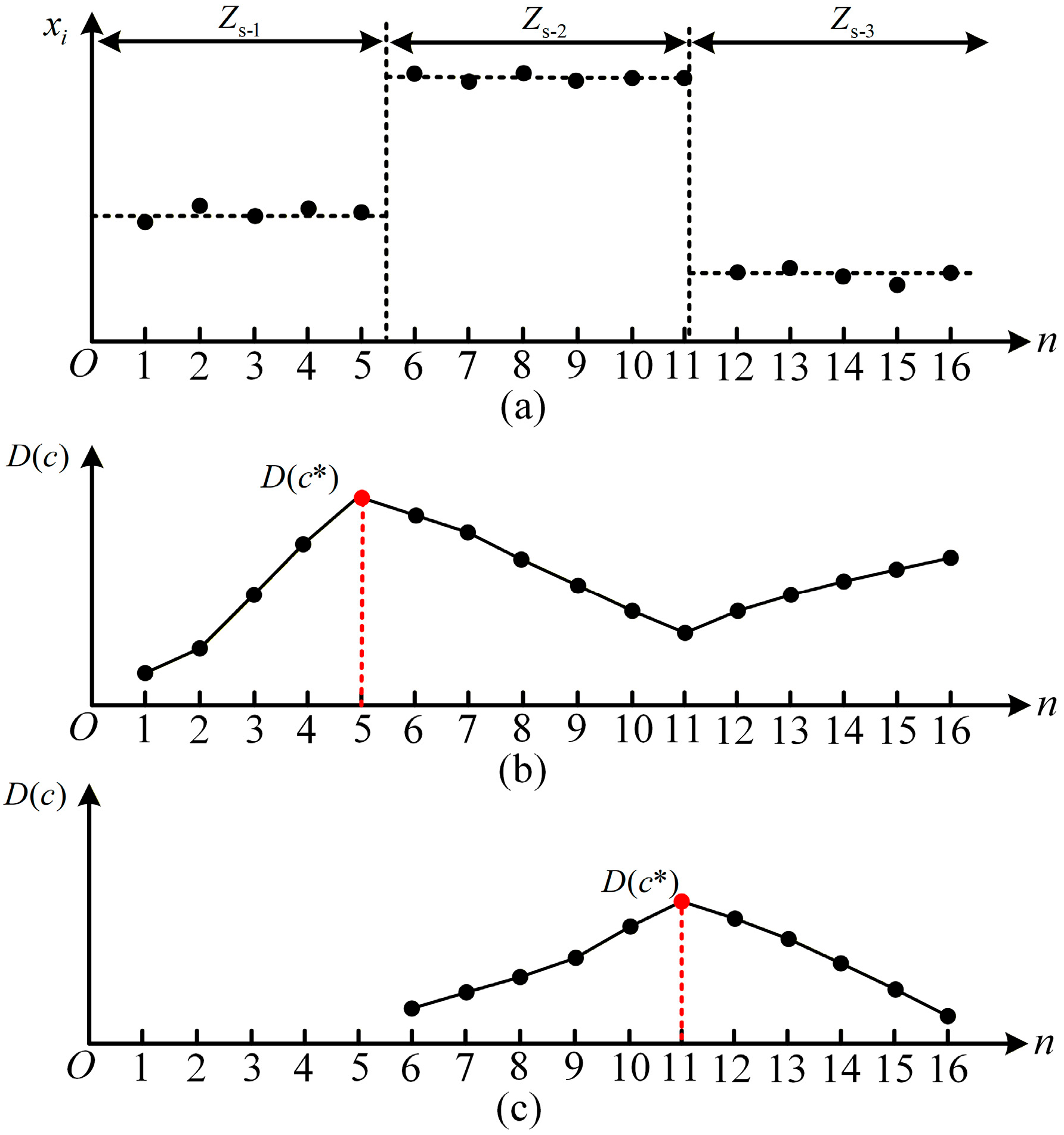
As shown in Figure 7a, the approximate harmonic impedance magnitude sequence can be regarded as several segments with relatively stable statistical characteristics. When the utility impedance changes, the statistical properties of the sequence also change, resulting in different impedance levels in different segments.

Figure 7. Diagram of the BG-based impedance abrupt change detection principle. (a) Approximate harmonic impedance magnitude sequence. (b) Result of the first impedance abrupt change detection. (c) Second impedance abrupt change detection result after sequence segmentation.

To detect the change point, the BG method filters the sequence and tentatively divides the data into two parts at each possible position. For each candidate division point, the statistical difference between the two segments is evaluated. By repeating this process for all possible positions, a statistic D(c) is obtained, as shown in Figure 7b. The position corresponding to the maximum value of D(c*) indicates the most significant statistical difference between the two subsequences and is therefore regarded as the most likely change point.

If the detected change point satisfies the statistical significance criterion, the sequence is split at this location. The same procedure is then recursively applied to the resulting subsequences until no further significant segmentation can be found. In this way, the impedance sequence can be divided into several segments with relatively stable characteristics, and the boundaries between segments correspond to the impedance change points, as illustrated in Figure 7c.

The key advantages of the BG method are its adaptive detection capability and independence from a priori assumptions about the number of change points. In harmonic impedance analysis, the impedance typically remains relatively stable before and after a change point, making the BG method effective for accurately identifying these abrupt variations, thereby providing a reliable basis for subsequent impedance modeling and system state analysis.

5. Simulation Results of Harmonic Impedance Estimation

In this section, the proposed method is rigorously tested using a MATLAB/Simulink 2020a multi-harmonic source model. The objective is to verify the algorithm’s accuracy and robustness under controlled scenarios with known true values.

5.1. Simulation Parameter Settings

To validate the efficacy and robustness of the proposed harmonic impedance estimation method, a comprehensive multi-harmonic source power system model is constructed in MATLAB/Simulink, as illustrated in Figure 8. The analysis primarily focuses on the fifth harmonic as a representative case.

Figure 8. Multi-harmonic source system.

The simulation spans 15 s, during which the utility harmonic impedance is programmed to change stepwise every 5 s to simulate typical grid transients. The specific parameters are configured as follows

(1)

Background harmonic voltage source: ${\dot{U}}_{\mathrm{s}}=40\angle {40}^{\circ }\mathrm{V}$. A random disturbance of ±30% is applied to the magnitude, and a random disturbance of ±15% is applied to the phase angle.

(2)

Utility harmonic impedance: 0~5 s, Z_s = (4.99 + j7.5) Ω; 5~10 s, Z_s = (7.5 + j10) Ω; 10~15 s, Z_s = (5 + j2.5) Ω.

(3)

Customer harmonic voltage sources: ${\dot{U}}_{\mathrm{c}1}=1000\angle {65}^{\circ }\mathrm{V}$; ${\dot{U}}_{\mathrm{c}2}=800\angle {55}^{\circ }\mathrm{V}$; ${\dot{U}}_{\mathrm{c}3}=600\angle {75}^{\circ }\mathrm{V}$.

(4)

Customer harmonic impedances: Z_c1 = (50 + j80) Ω; Z_c2 = (30 + j50) Ω; Z_c3 = (40 + j70) Ω.

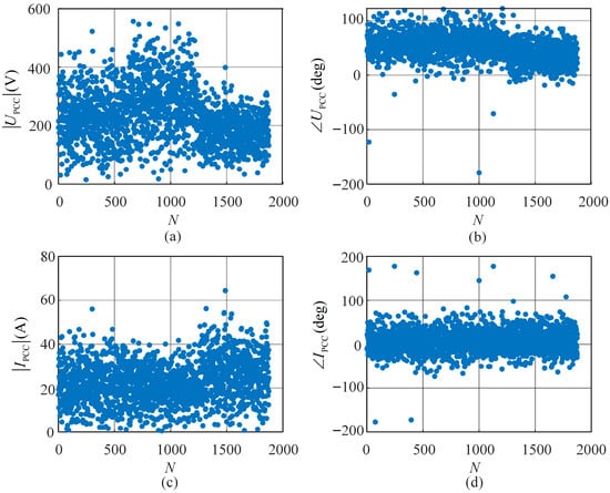
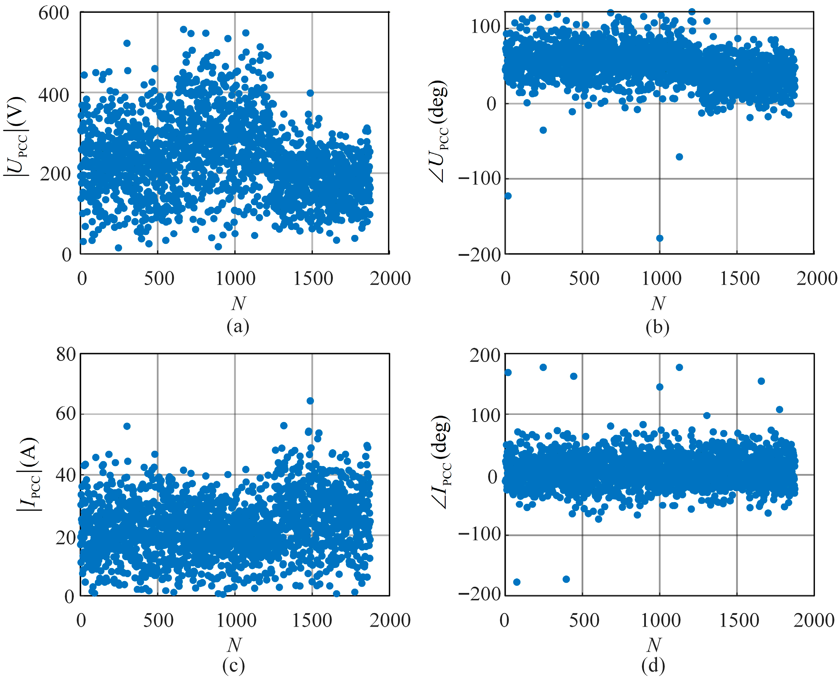
Table 1 presents the key parameters of the method proposed in this paper. A total of 1875 sets of fifth-harmonic voltage and current data at the PCC are obtained in the simulation experiment, and their magnitudes and phase angles are shown in Figure 9. As shown in Figure 9, the harmonic data are disordered and cannot be directly used to calculate the utility harmonic impedance using the bivariate linear regression method.

Table 1. The key parameters of the proposed method.

Parameter	Symbol	Value
Window length	L	20
Sliding step	s	5
Linearity threshold	Ft	50
The number of trees	/	100
Confidence level threshold	P0	0.95

Figure 9. The fifth-harmonic data at the PCC. (a) Harmonic voltage magnitude. (b) Harmonic voltage phase angle. (c) Harmonic current magnitude. (d) Harmonic current phase angle.

5.2. Harmonic Data Filtering Based on the Sliding-Window-Based Isolation Forest Method

First, the sliding-window-based IF method is used to filter the harmonic data. A sliding window with a window length of 20 and a sliding step size of 5 is constructed. The data segments with F > 50 are selected using the F-statistic, and then the IF method is employed to remove outliers in the harmonic data sequence. Approximately 3% of the original data points are identified as outliers and removed by the IF. The remaining data retain sufficient quantity and quality to ensure reliable estimation results.

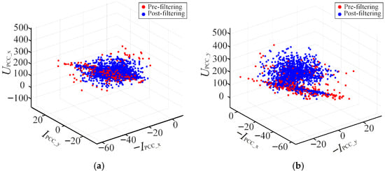
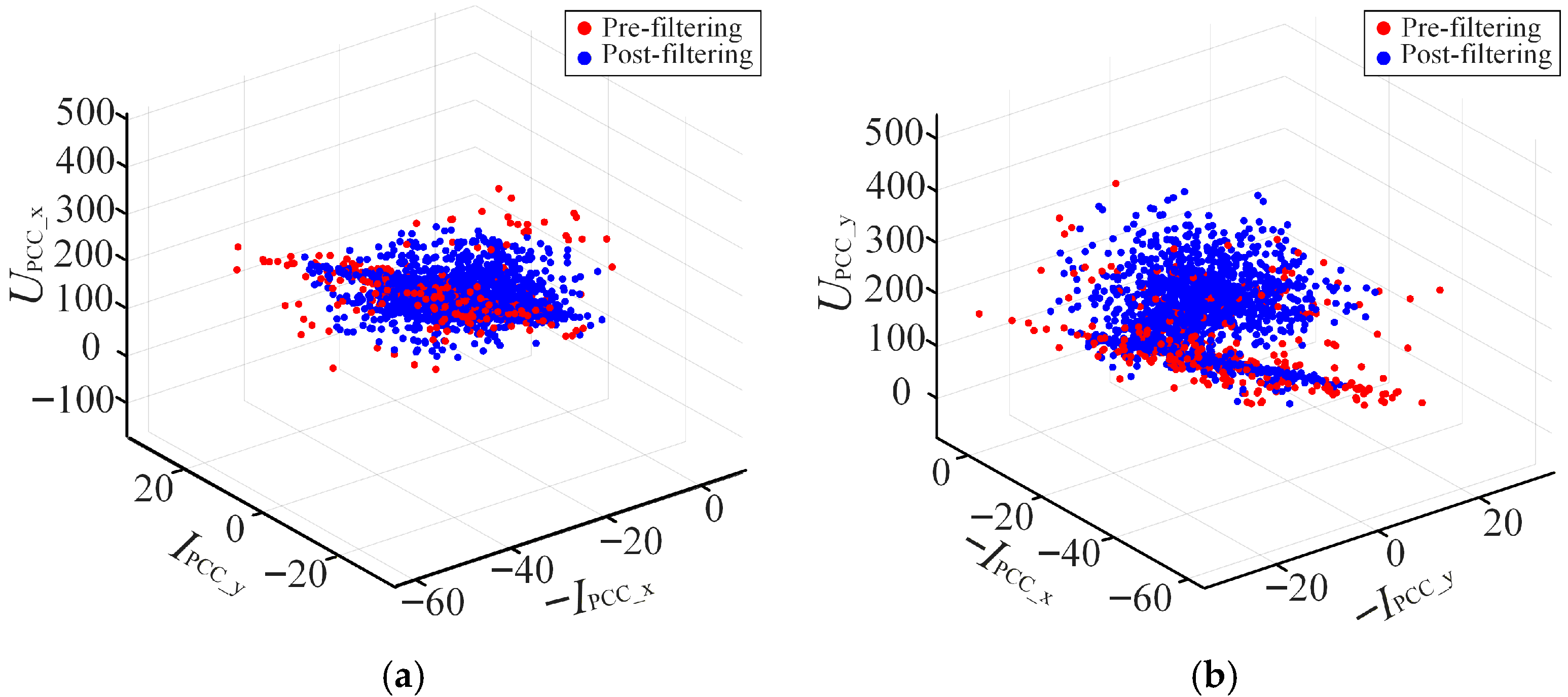
According to (16), the three-dimensional scatter plot of the harmonic data is constructed, as shown in Figure 10. From Figure 10, due to the fluctuation of the background harmonic voltage, it is difficult to observe a clear linear relationship in the data before filtering. After filtering, the data are distributed on several planes. According to the theoretical analysis presented above, the filtered harmonic voltage and current data exhibit a strong correlation, indicating that the background harmonic voltage is relatively stable. The reason why the data lie on multiple planes is that abrupt changes in harmonic impedance occur, and each plane represents a different utility harmonic impedance.

Figure 10. Scatter plot comparison before and after filtering. (a) (U_{PCC_x}, I_{PCC_y}, −I_{PCC_x}). (b) (U_{PCC_y}, −I_{PCC_x}, −I_{PCC_y}).

5.3. Impedance Change Points Detection Based on the BG Method

Since abrupt changes occur in the harmonic impedance, the filtered harmonic data cannot be directly processed using the bivariate linear regression method. Therefore, the BG method is employed to detect the abrupt change points of the harmonic impedance.

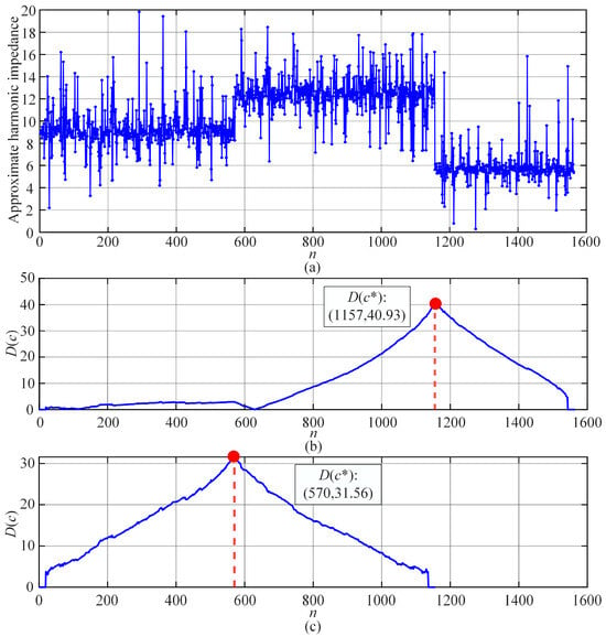
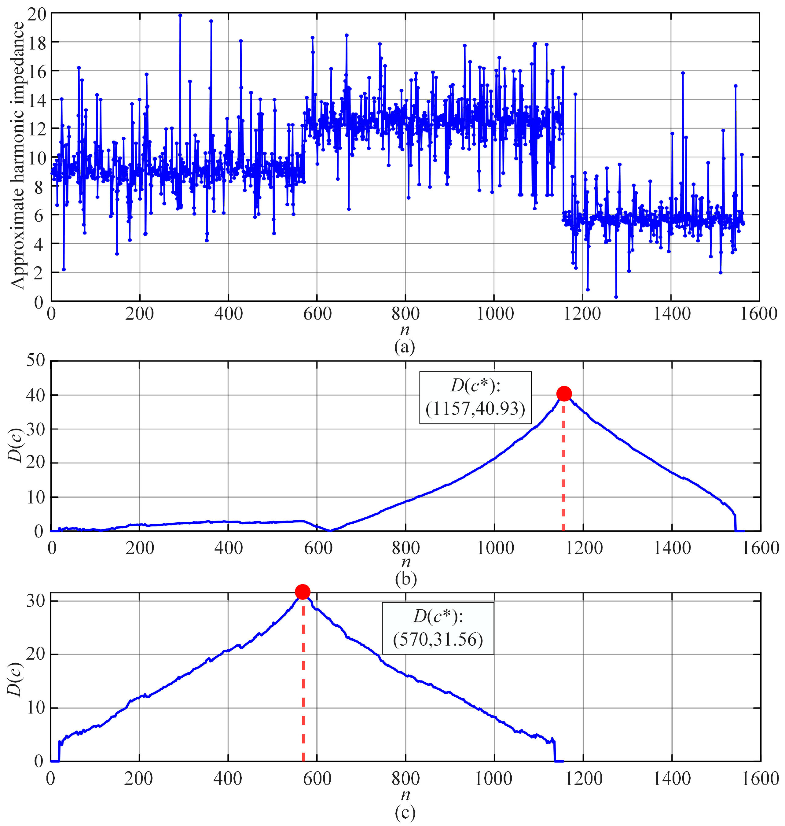
According to (23), the two-point method is used to approximately estimate the magnitude of the utility harmonic impedance, and the results are shown in Figure 11a. The harmonic impedance magnitude clearly exhibits three segments, indicating that two abrupt changes have occurred.

Figure 11. Impedance change point detection results. (a) Approximate harmonic impedance magnitude sequence. (b) Result of the first impedance abrupt change detection. (c) Second impedance abrupt change detection result after sequence segmentation.

The BG method detects the impedance abrupt change points based on a mean-shift detection criterion. In the first detection, the maximum standardized mean appears at n = 1157, as shown in Figure 11b. The sequence is then segmented at this point, and the BG method is applied again to the resulting subsequence. In the second detection, the maximum standardized mean occurs at n = 570, which exactly corresponds to the change instant set in the simulation of this paper. These results demonstrate that the BG method can effectively identify the impedance abrupt change points.

5.4. Harmonic Impedance Estimation Results Based on Bivariate Linear Regression

Based on the abrupt change detection results obtained by the BG method, the harmonic data are divided into three groups. The harmonic impedance of each group is then estimated using the bivariate linear regression method. The estimation results are presented in Table 2 and Table 3. The confidence intervals of the impedance estimation results reported in the tables are at the 95% level.

Table 2. Estimated real part of utility harmonic impedance.

Methods	Parameters	Time Interval
		0~5 s	5~10 s	10~15 s
FLU method	Estimated value/Ω	4.32	8.68	4.17
	Relative error/%	13.45	15.68	16.55
LR method	Estimated value/Ω	5.52	8.24	5.58
	Relative error/%	10.53	9.88	11.63
ICA method	Estimated value/Ω	4.56	6.94	4.51
	Relative error/%	8.64	7.53	9.84
IRV method	Estimated value/Ω	5.32	6.95	5.27
	Relative error/%	6.65	7.34	5.36
The proposed	Estimated value/Ω	4.90	7.66	5.10
	Relative error/%	1.85	2.16	1.93
Comparison	True value/Ω	4.99	7.5	5

Table 3. Estimated imaginary part of utility harmonic impedance.

Methods	Parameters	Time Interval
		0~5 s	5~10 s	10~15 s
FLU method	Estimated value/Ω	8.51	8.45	2.87
	Relative error/%	13.53	15.47	14.88
LR method	Estimated value/Ω	6.61	11.03	2.27
	Relative error/%	11.89	10.32	9.15
ICA method	Estimated value/Ω	6.88	10.79	2.72
	Relative error/%	8.31	7.85	8.96
IRV method	Estimated value/Ω	8.05	9.20	2.66
	Relative error/%	7.32	8.05	6.21
The proposed	Estimated value/Ω	7.40	10.21	2.46
	Relative error/%	1.31	2.05	1.58
Comparison	True value/Ω	7.5	10	2.5

We compare the proposed method with four other approaches: (1) the fluctuation (FLU) method [9], (2) the linear regression (LR) method [11], (3) the ICA method [17], (4) the independent random vector (IRV) method [18], and (5) the proposed method. The FLU method evaluates harmonic impedance by taking the ratio of the incremental changes in harmonic voltage to harmonic current. The LR method determines harmonic impedance through the calculation of regression coefficients. The ICA method estimates harmonic impedance by separating signals, leveraging the weak correlation between harmonic sources from the utility and the customer sides. The IRV method derives the utility harmonic impedance by utilizing the weak correlation between the harmonic current and the background harmonic voltage.

From Figure 12, the proposed method achieves the lowest relative errors (RE), consistently remaining below 2.2% for both real and imaginary parts across all time intervals. While traditional methods (FLU, LR) exhibit significant errors (often exceeding 10%). The FLU and LR methods are global calculation techniques. They assume that the background harmonic voltage and utility impedance remain constant over the entire measurement window. When applied to real-world data with abrupt impedance changes, these methods fit a single erroneous average across multiple operating states, leading to massive Res [25]. The ICA and IRV methods rely heavily on the statistical assumption that utility-side and customer-side harmonics are strictly independent. In heavily interconnected grids with multi-harmonic sources, this weak correlation assumption frequently breaks down [26]. The proposed method does not rely on this assumption; instead, it dynamically segments the data into piecewise stationary states using the BG method, ensuring that local linear regressions are applied only to strictly valid, strongly correlated data subsets.

Figure 12. Comparison of relative error for different methods. (a) Comparison of relative errors of the real part of harmonic impedance. (b) Comparison of relative errors of the imaginary part of harmonic impedance.

To demonstrate the robustness of the proposed method, a dedicated sensitivity analysis has been added using simulation data with different signal-to-noise ratios (SNRs), ranging from 10 dB to noise-free conditions (∞). This setting is used to emulate different levels of measurement uncertainty.

As shown in Table 4, the REs of the 5th harmonic impedance estimation gradually increase as the noise level increases (i.e., SNR decreases). However, even under severe noise conditions (10 dB), the estimation errors remain within an acceptable range (below 3%), demonstrating the robustness of the proposed method against measurement noise.

Table 4. Relative errors for 5th harmonic impedance estimation at different SNRs. (average value for 100 trials).

0~5 s Impedance	RE for Different SNR (%)
	10 dB	20 dB	30 dB	∞ (No Noise)
5-Zs-Re	2.81	2.28	2.11	1.77
5-Zs-Im	2.16	1.75	1.58	1.32

6. Field Application Results

To demonstrate the practical utility of the proposed framework, this section applies the method to field measurement data from a 500 kV HVDC converter station, comparing its performance against established industrial standards.

To evaluate the practical applicability of the proposed method, it is further validated using field measurement data that inherently include various non-ideal factors encountered in real operating environments, such as measurement noise. The dataset used in this study was collected from the 500 kV busbar of an HVDC converter station located in southern China. The converter station adopts a 3/2 busbar configuration and is connected to eight transmission lines as well as four groups of AC filters. Although the control dynamics of the power electronic converters and their detailed impedance characteristics are not explicitly modeled in this work, their influence on harmonic impedance is implicitly reflected in the measured data.

The proposed method is not specifically tuned for the 500 kV system but is kept consistent across all cases based on general guidelines. The filtering strategy does not treat all harmonic variations as noise; instead, it preserves physically meaningful dynamics in HVDC systems while removing only those data that violate the voltage–current relationship required for impedance estimation.

6.1. Experimental Setup and Standards

The voltage and current at the point of common coupling (PCC) are synchronously recorded using a power quality analyzer compliant with the requirements of IEC 61000-4-7 [27]. The sampling frequency is set to 6400 Hz, and the harmonic components of voltage and current, including their phase angles, are extracted through fast Fourier transform (FFT). In accordance with IEC 61000-4-7, the FFT window length is selected as 10 cycles (0.2 s in a 50-Hz system) with a rectangular window. To mitigate the impact of random measurement errors, the computed harmonic quantities are averaged over a one-second interval, yielding a total of 2880 samples. In addition, the harmonic phase angles are referenced to the fundamental voltage to eliminate phase deviations caused by slight variations in the fundamental frequency.

The current transformer (CT) and capacitive voltage transformer (CVT) used in the measurement system are rated as Class 0.2 according to IEC 60044-1 [28] and IEC 60044-5 [29] (superseded by IEC 61869-2 [30] and IEC 61869-5 [31]). However, it should be noted that this accuracy class is specified only within the frequency range of 15–100 Hz. In practice, CVTs tend to exhibit larger errors at higher frequencies compared with CTs. Therefore, a parameter identification approach is employed in this study to compensate for the CVT ratio error, enabling accurate harmonic voltage measurements up to the 50th harmonic order in accordance with IEC 61000-4-7.

6.2. Data Acquisition and Preprocessing

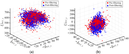
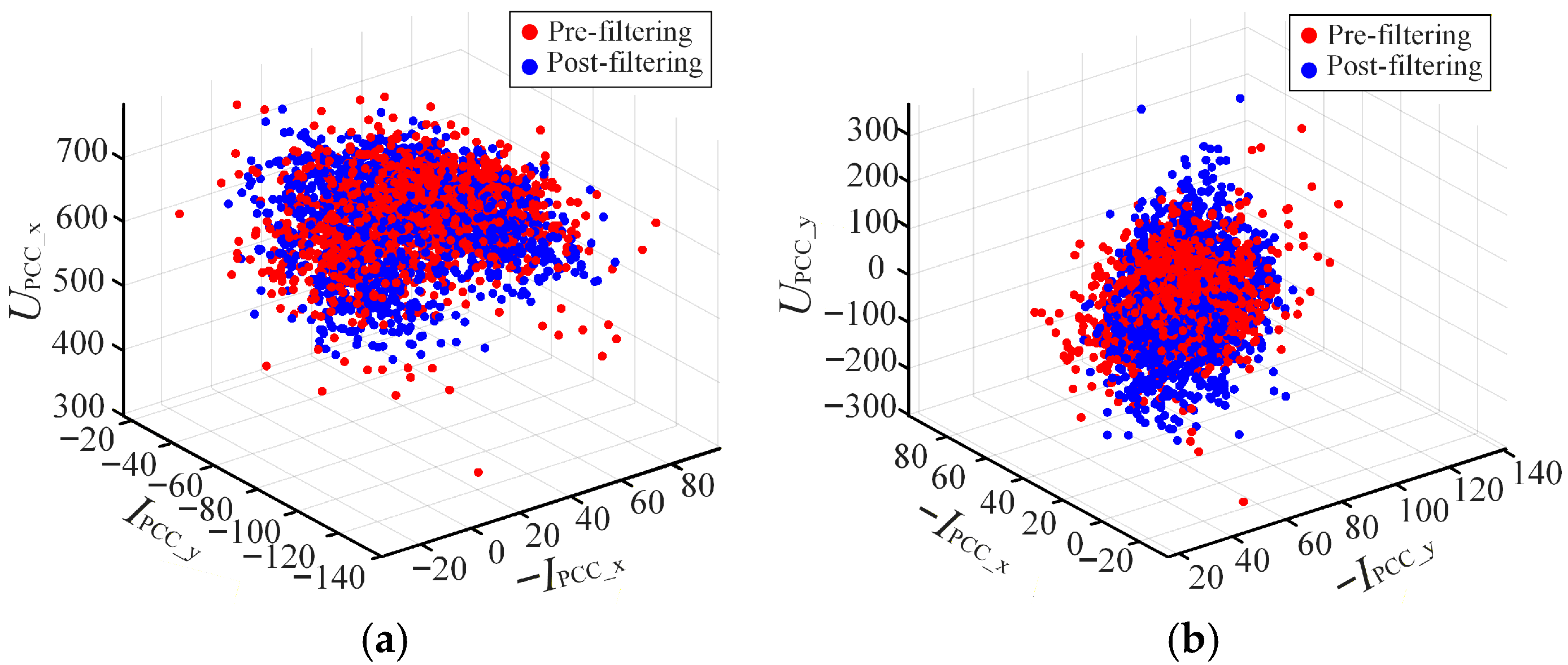
The sliding-window-based IF method is first used to filter the raw field data. The three-dimensional scatter plots of the harmonic data before and after filtering are illustrated in Figure 13. The data points appear disordered and scattered due to the inherent measurement noise and random fluctuations of the background harmonic voltage. After applying the proposed method, the filtered data exhibit a distinct layered distribution, concentrated on three separate planes. This clustering indicates that the background harmonic voltage remained relatively stable during the selected intervals, while the utility harmonic impedance underwent discrete state changes.

Figure 13. Scatter plot comparison before and after filtering. (a) (U_{PCC_x}, I_{PCC_y}, −I_{PCC_x}). (b) (U_{PCC_y}, −I_{PCC_x}, −I_{PCC_y}).

6.3. Impedance Change Point Detection

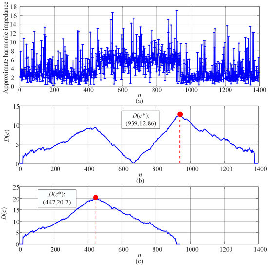
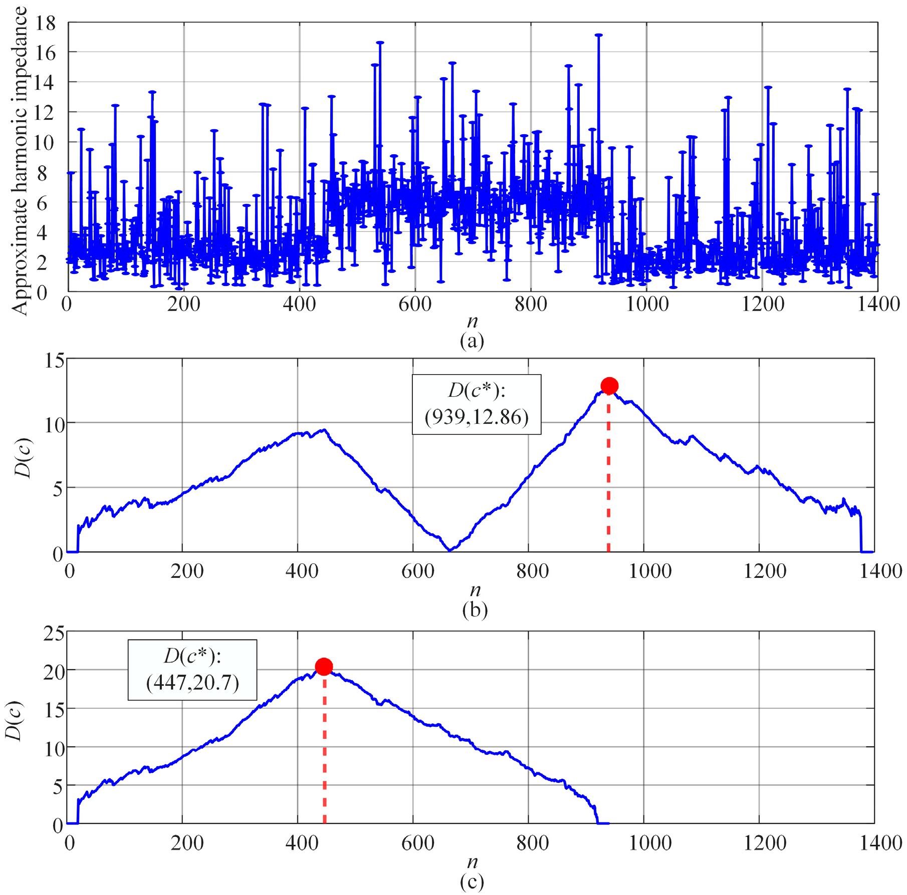
Given the observed abrupt changes in the data distribution, the BG method was utilized to identify the precise switching instants. The approximate harmonic impedance magnitude sequence is shown in Figure 14a.

Figure 14. Results of harmonic impedance change point detection. (a) Approximate harmonic impedance magnitude sequence. (b) Result of the first impedance abrupt change detection. (c) Second impedance abrupt change detection result after sequence segmentation.

The first abrupt change is detected at n = 939, where the standardized mean reached its maximum. After segmenting the sequence, a second change point is identified at n = 447. Based on these detection results, the measurement period is divided into three intervals corresponding to specific grid operating conditions.

The detected change points are unlikely to be false positives caused by transient oscillations, since the BG method is based on a mean-change detection principle. Specifically, it identifies impedance changes by detecting statistically stable shifts in the mean behavior of the data over a period of time. Therefore, a valid change point must exhibit a sustained deviation across consecutive samples [32,33]. In contrast, transient oscillations typically present as short-duration, zero-mean fluctuations and do not satisfy this persistence condition, making them unlikely to be identified as change points by the proposed method.

6.4. Comparative Analysis of Estimation Results

Following the segmentation, the harmonic impedance for each interval is estimated using the bivariate linear regression method. The proposed method is compared against four established techniques: the FLU method, LR method, ICA method, and IRV method.

In practical power systems, the true value of the equivalent utility harmonic impedance cannot be directly measured due to unknown parameters of field components and the influence of frequency-dependent effects such as the skin effect. Therefore, in this study, a controlled disturbance-based approach is adopted to obtain a reference value. Specifically, a large load on the customer side is intentionally switched off, which induces a significant and observable change in both harmonic voltage and current. Based on the measured variations before and after the switching event, the reference harmonic impedance is calculated as

$$Z_{\mathrm{s}\_\mathrm{ref}}^h={\displaystyle \frac{{\dot{U}}_{\mathrm{PCC}\left(\mathrm{after}\right)}^h-{\dot{U}}_{\mathrm{PCC}\left(\mathrm{before}\right)}^h}{{\dot{I}}_{\mathrm{PCC}\left(\mathrm{after}\right)}^h-{\dot{I}}_{\mathrm{PCC}\left(\mathrm{before}\right)}^h}}$$

(30)

where ${\dot{U}}_{\mathrm{PCC}}^h$ and ${\dot{I}}_{\mathrm{PCC}}^h$ are the values before and after switching off the load.

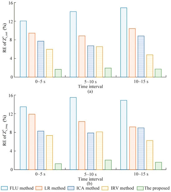
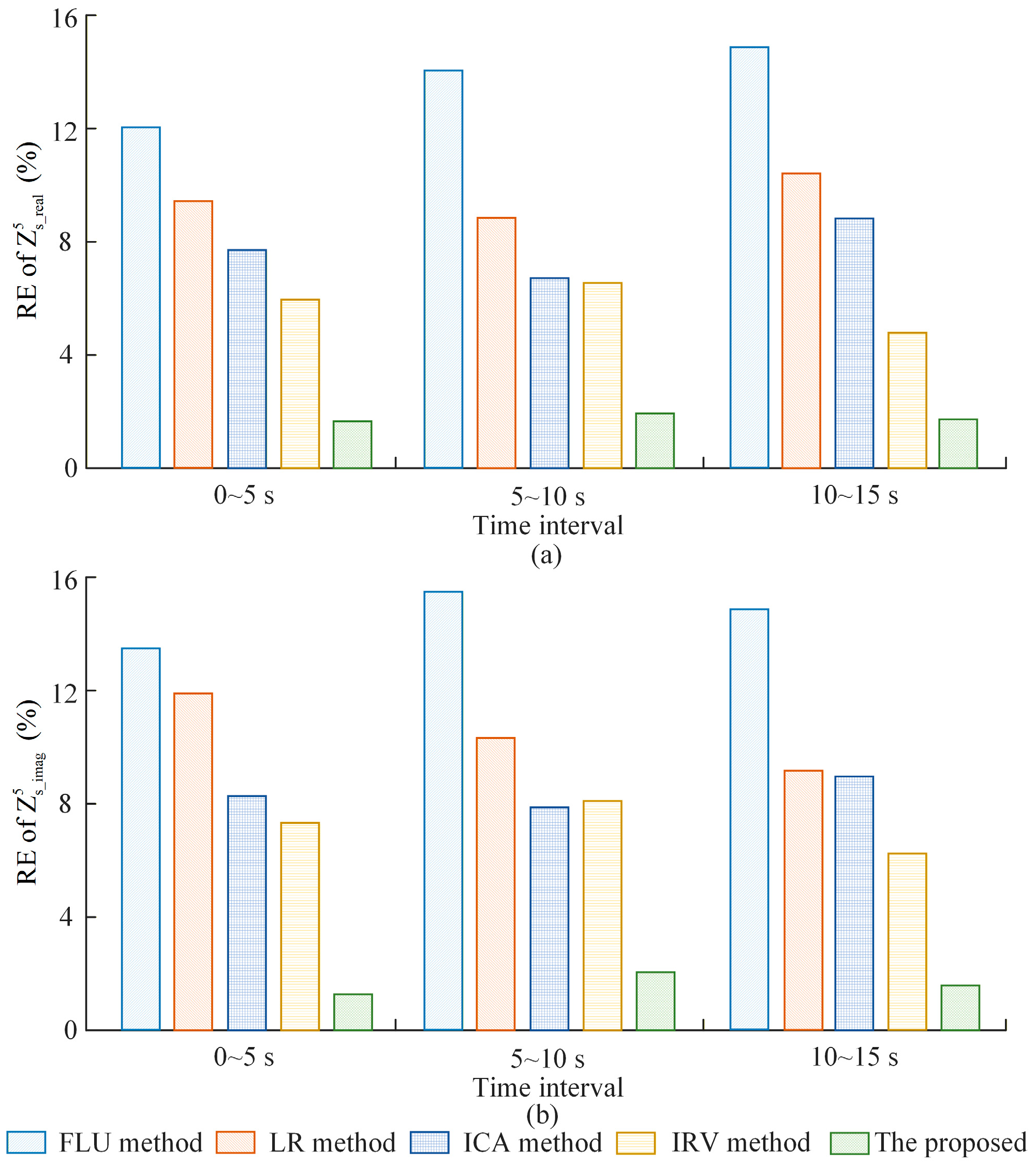
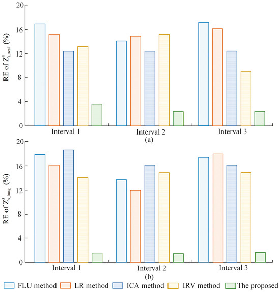
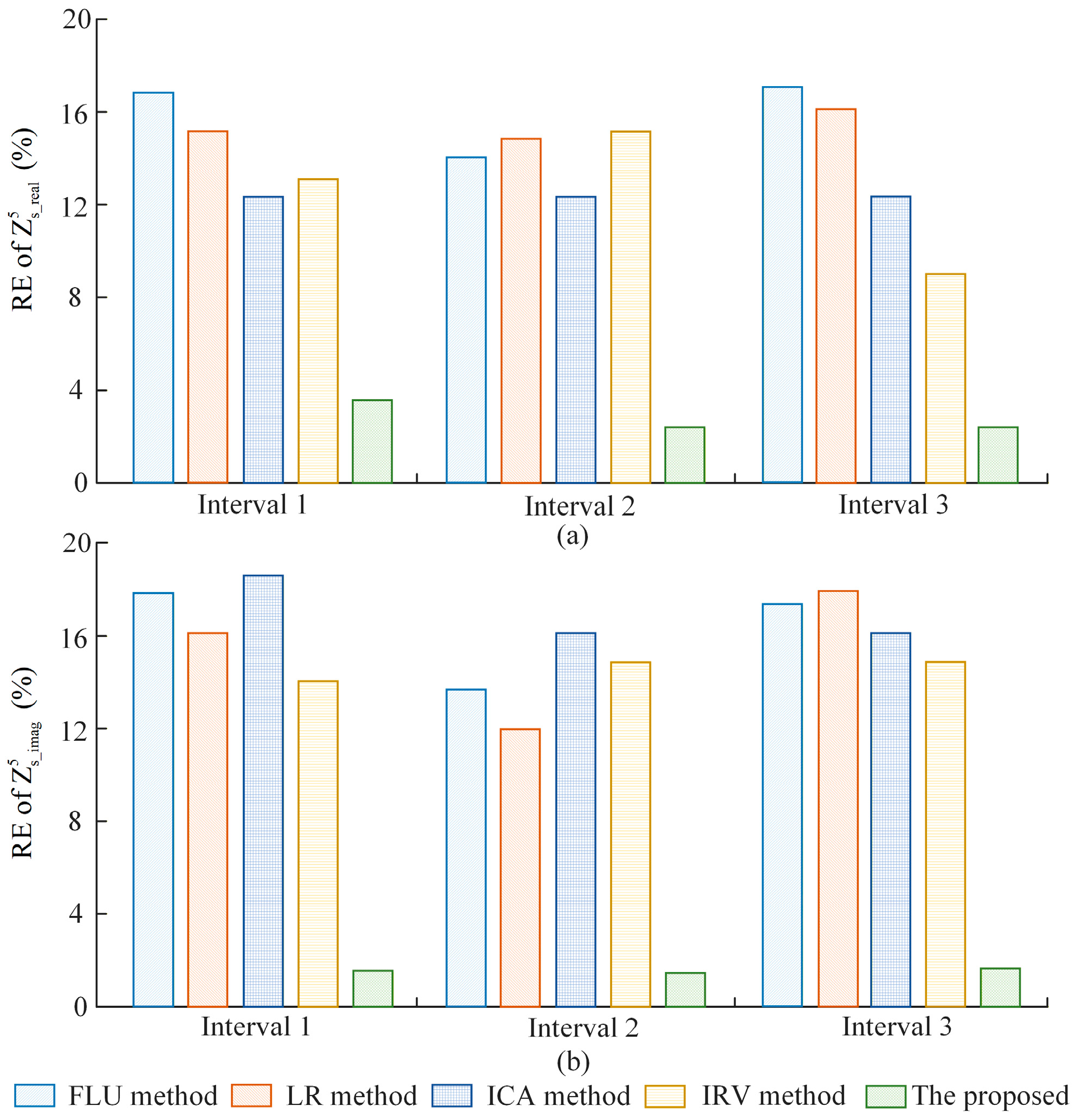
The RE comparisons for the real and imaginary parts of the estimated impedance are presented in Figure 15. The FLU and LR methods exhibited significantly higher errors, often exceeding 12% in real-world conditions, as they are highly sensitive to background harmonic fluctuations. By effectively filtering disturbances and accurately identifying impedance transition points, the proposed method achieves the highest precision across all three intervals. The relative errors for both the real and imaginary components remain consistently low, significantly outperforming the comparative algorithms.

Figure 15. Relative errors of the 5th harmonic impedance. (a) Real part. (b) Imaginary part.

According to IEC 61000-4-7, the maximum allowable error for Class I harmonic measurement instruments is approximately 5% for voltage and current. Our proposed method achieves a relative error of less than 4%. This demonstrates that the computational error introduced by our estimation algorithm is lower than the inherent measurement tolerance of standard PQ instruments, ensuring that the algorithm does not become the bottleneck of the overall measurement chain.

In practical power system engineering, especially for harmonic responsibility allocation, an estimation error within 10% is generally considered acceptable for identifying dominant harmonic sources and implementing mitigation strategies. Our result (<4%) significantly exceeds this requirement, providing high-confidence data for utility-customer dispute resolution and filter design.

These field results demonstrate that the proposed algorithm is highly effective for harmonic impedance estimation in practical engineering applications. All simulations and field data processing were performed on a workstation equipped with an Intel Core i7-14700 CPU @ 2.10 GHz and 32 GB RAM. Both simulation and experimental results indicate that the total computation time for harmonic impedance estimation remains below 1 s. This indicates that the proposed method has a low computational burden and can be efficiently implemented in practice.

6.5. Uncertainty Analysis

(1) Measurement uncertainty

A source of measurement uncertainty might arise from the limitations of harmonic measurement instruments. Current CTs and CVTs are primarily designed for fundamental frequency, making it difficult to accurately measure harmonic data.

At high frequencies, magnetic saturation and leakage inductance in CTs can result in phase and amplitude errors in the measured harmonic currents. Additionally, the nonlinear properties of the CT core material and parasitic parameters further affect the transmission and response characteristics of high-frequency harmonics. For CVTs, although its frequency response is corrected in this study, the laboratory experiments cannot fully replicate the field environment. Variations in temperature, humidity, or electromagnetic interference in field applications can alter the CVT’s frequency response.

(2) Limitations on the proposed method

The accuracy of the proposed method primarily depends on the correlation between ${\dot{I}}_{\mathrm{PCC}}^h$ and ${\dot{U}}_{\mathrm{PCC}}^h$. If the customer-side harmonic impedance $Z_{\mathrm{c}}^h$ is infinite, ${\dot{I}}_{\mathrm{PCC}}^h$ and ${\dot{U}}_{\mathrm{PCC}}^h$ exhibit a strong positive correlation. Under such conditions, the proposed method can provide accurate probabilistic estimations, irrespective of fluctuations in the background harmonic voltage. In most practical cases, $Z_{\mathrm{c}}^h$ is finite but significantly larger than $Z_{\mathrm{s}}^h$, which allows the proposed method to give accurate estimation results. However, if capacitors or harmonic filters are installed on the customer side, the condition that $Z_{\mathrm{c}}^h$ is much larger than $Z_{\mathrm{s}}^h$ may be violated, thereby affecting the accuracy of the estimation.

7. Conclusions

This paper proposes a noninvasive harmonic impedance estimation method based on the IF and BG algorithms. The proposed approach effectively mitigates the influence of background harmonic voltage fluctuations and abrupt impedance variations, thereby improving both the accuracy and robustness of utility harmonic impedance estimation.

Simulation and field validation results demonstrate that the proposed method achieves consistently low estimation errors, with relative errors maintained below 4% under both steady-state and disturbance conditions. Compared with conventional approaches, the proposed framework exhibits superior performance in handling non-stationary operating scenarios. Specifically, the IF-based filtering stage enhances data quality by eliminating noise-contaminated samples, while the BG-based segmentation enables accurate detection of impedance change points and ensures piecewise-stationary regression.

From a practical perspective, the proposed method provides a more reliable basis for harmonic responsibility allocation and power quality assessment in modern power systems with high renewable energy penetration. The applicability of the method is particularly relevant to HVDC systems and distribution networks characterized by frequent harmonic interactions and switching-induced impedance variations.

However, several limitations should be noted. Under extremely strong background harmonic fluctuations, the effective data availability may be reduced, which can affect estimation stability. In addition, the recursive structure of the BG method and the ensemble-based nature of IF increase computational complexity, which may limit real-time applicability in ultra-fast dynamic scenarios. Furthermore, performance may degrade under highly time-varying operating conditions, and appropriate parameter tuning is still required for different system environments.

Future research will focus on reducing computational burden through algorithmic optimization, improving real-time performance, and developing adaptive parameter selection strategies (e.g., window length and step size) to enhance robustness under faster transient conditions.

References

- Chakravorty, D.; Meyer, J.; Schegner, P.; Yanchenko, S.; Schocke, M. Impact of Modern Electronic Equipment on the Assessment of Network Harmonic Impedance. IEEE Trans. Smart Grid 2017, 8, 382–390. [Google Scholar] [CrossRef] [Scilit]
- Xu, F.; Yang, H.; Zhao, J.; Wang, Z.; Liu, Y. Study on Constraints for Harmonic Source Determination Using Active Power Direction. IEEE Trans. Power Deliv. 2018, 33, 2683–2692. [Google Scholar] [CrossRef] [Scilit]
- Liu, T.; Shu, Q.; Xu, F.; Fan, L.; Li, H. A Method for Determining Harmonic Contribution and Harmonic Source Current Based on Minimum Mutual Information and Bayesian Optimization. IEEE Trans. Instrum. Meas. 2024, 73, 1–8. [Google Scholar] [CrossRef] [Scilit]
- Xiao, X.; Li, Z.; Wang, Y.; Zhou, Y. A Practical Approach to Estimate Harmonic Distortions in Residential Distribution System. IEEE Trans. Power Deliv. 2021, 36, 1418–1427. [Google Scholar] [CrossRef] [Scilit]
- Fan, Y.; Xu, F.; Wang, C.; Shu, Q. A Harmonic Impedance on Utility Side Estimation Method Based on Laplace Mixture Model. IEEE Trans. Power Deliv. 2024, 39, 1774–1782. [Google Scholar] [CrossRef] [Scilit]
- Zhou, R.; Ma, X.; Xu, R.; Xiao, X.; Zhao, J. Novel Method for Estimating Utility Harmonic Impedance for a Direct-Drive Permanent Magnet Synchronous Generator Wind Farm. IEEE Access 2022, 10, 25872–25882. [Google Scholar] [CrossRef] [Scilit]
- Monteiro, H.L.M.; Duque, C.A.; Silva, L.R.; Meyer, J.; Stiegler, R.; Testa, A.; Ribeiro, P.F. Harmonic impedance measurement based on short time current injections. Electr. Power Syst. Res. 2017, 148, 108–116. [Google Scholar] [CrossRef] [Scilit]
- Shu, Q.; Wu, Y.; Xu, F.; Zheng, H. Estimate Utility Harmonic Impedance via the Correlation of Harmonic Measurements in Different Time Intervals. IEEE Trans. Power Deliv. 2020, 35, 2060–2067. [Google Scholar] [CrossRef] [Scilit]
- He, Z.-Y.; Chen, J.; Fu, L.; Zang, T.-L. Harmonic contribution assessment on the condition of background harmonic fluctuations. In Proceedings of the 2015 International Symposium on Smart Electric Distribution Systems and Technologies (EDST), Vienna, Austria, 8–11 September 2015; pp. 431–435. [Google Scholar]
- Xu, W.; Ahmed, E.E.; Zhang, X.; Liu, X. Measurement of network harmonic impedances: Practical implementation issues and their solutions. IEEE Trans. Power Deliv. 2002, 17, 210–216. [Google Scholar] [CrossRef] [Scilit]
- Xia, Y.; Tang, W. Study on the estimation of harmonic impedance based on Bayesian optimized Gaussian process regression. Int. J. Electr. Power Energy Syst. 2022, 142, 108294. [Google Scholar] [CrossRef] [Scilit]
- Shu, Q.; Liu, T.; Xue, F. A new algorithm for calculating utility harmonic impedance. Electr. Power Syst. Res. 2021, 191, 106893. [Google Scholar] [CrossRef] [Scilit]
- Hui, J.; Freitas, W.; Vieira, J.C.M.; Yang, H.; Liu, Y. Utility Harmonic Impedance Measurement Based on Data Selection. IEEE Trans. Power Deliv. 2012, 27, 2193–2202. [Google Scholar] [CrossRef] [Scilit]
- Shu, Q.; Fan, Y.; Xu, F.; Wang, C.; He, J. A harmonic impedance estimation method based on AR model and Burg algorithm. Electr. Power Syst. Res. 2022, 202, 107568. [Google Scholar] [CrossRef] [Scilit]
- Hua, H.; Jia, X.; Cao, D.; Zhao, C. Practical method to determine the harmonic contribution of a specific harmonic load. In Proceedings of the 2012 IEEE 15th International Conference on Harmonics and Quality of Power, Hong Kong, China, 17–20 June 2012; pp. 769–773. [Google Scholar]
- Zheng, X.; Xiao, X.; Wang, Y. Harmonic impedance measurement based on an improved binary regression algorithm and dynamic time warping distance. Int. J. Electr. Power Energy Syst. 2021, 130, 106907. [Google Scholar] [CrossRef] [Scilit]
- Karimzadeh, F.; Esmaeili, S.; Hosseinian, S.H. A Novel Method for Noninvasive Estimation of Utility Harmonic Impedance Based on Complex Independent Component Analysis. IEEE Trans. Power Deliv. 2015, 30, 1843–1852. [Google Scholar] [CrossRef] [Scilit]
- Hui, J.; Yang, H.; Lin, S.; Ye, M. Assessing Utility Harmonic Impedance Based on the Covariance Characteristic of Random Vectors. IEEE Trans. Power Deliv. 2010, 25, 1778–1786. [Google Scholar] [CrossRef] [Scilit]
- Liu, Z.; Xu, Y.; Jiang, H.; Tao, S. Study on Harmonic Impedance Estimation and Harmonic Contribution Evaluation Index. IEEE Access 2020, 8, 59114–59125. [Google Scholar] [CrossRef] [Scilit]
- Li, W.; Wang, S.; Tu, H.; Miao, H.; Jiao, N.; Liu, T. Utility harmonic impedance estimation based on time series clustering and improved Pettitt method. Int. J. Electr. Power Energy Syst. 2025, 170, 110935. [Google Scholar] [CrossRef] [Scilit]
- Ding, T.; Zhu, M.; Yi, W.; Gao, M.; Jiao, Y.; Wei, Q. Utility harmonic impedance estimation considering unsmooth fluctuation characteristics of background harmonics. Electr. Power Syst. Res. 2025, 243, 111513. [Google Scholar] [CrossRef] [Scilit]
- Xu, F.; Wang, C.; Shu, Q.; Ma, Z.; Zheng, H.; Peng, A. Study on the Estimation of Utility Harmonic Impedance Based on Minimum Norm of Impedance Difference. IEEE Access 2020, 8, 207389–207396. [Google Scholar] [CrossRef] [Scilit]
- Li, Y.; Duan, Y.; Bao, C.; Hou, Y.; Zhang, L. Harmonic Impedance Estimation Method Based on Data Filtering and Improved Rank Regression. In Proceedings of the 2024 3rd Asian Conference on Frontiers of Power and Energy (ACFPE), Chengdu, China, 15–17 November 2024; pp. 716–723. [Google Scholar]
- Mazin, H.E.; Xu, W.; Huang, B. Determining the Harmonic Impacts of Multiple Harmonic-Producing Loads. IEEE Trans. Power Deliv. 2021, 26, 1187–1195. [Google Scholar]
- Zhang, J.; Jiang, D.; Liu, C. Dominant Harmonic Source Determination Based on Comprehensive Minimum Fluctuation. In Proceedings of the 2025 8th International Conference on Power and Energy Applications (ICPEA), Shanghai, China, 23–25 October 2025; pp. 341–346. [Google Scholar]
- da Cunha Gomes, F.; Sotelo, G.G.; França, B.W. Mitigation of Harmonic Distortion and Voltage Fluctuation from Portable Welding Machines in Shipboard Power Systems. In Proceedings of the 2025 Brazilian Power Electronics Conference (COBEP), Vitoria, Brazil, 5–8 October 2025; pp. 1–6. [Google Scholar]
- IEC 61000-4-7; Electromagnetic Compatibility (EMC)—Part 4-7: Testing and Measurement Techniques—General Guide on Harmonics and Interharmonics Measurements and Instrumentation, for Power Supply Systems and Equipment Connected Thereto. International Electrotechnical Commission: Geneva, Switzerland, 2002.
- IEC 60044-1; Instrument Transformers—Part 1: Current Transformers. International Electrotechnical Commission: Geneva, Switzerland, 2003.
- IEC 60044-5; Instrument Transformers—Part 5: Capacitor Voltage Transformers. International Electrotechnical Commission: Geneva, Switzerland, 2004.
- IEC 61869-2; Instrument Transformers—Part 2: Additional Requirements for Current Transformers. International Electrotechnical Commission: Geneva, Switzerland, 2012.
- IEC 61869-5; Instrument Transformers—Part 5: Additional Requirements for Capacitor Voltage Transformers. International Electrotechnical Commission: Geneva, Switzerland, 2011.
- Crepaldi, J.; Amoroso, M.M.; Ando, O.H. Analysis of the Topologies of Power Filters Applied in Distributed Generation Units—Review. IEEE Lat. Am. Trans. 2018, 16, 1892–1897. [Google Scholar] [CrossRef]
- Gimenes, T.K.; Da Silva, M.P.C.; Ledesma, J.J.G.; Ando, O.H., Jr. Impact of distributed energy resources on power quality: Brazilian scenario analysis. Electr. Power Syst. Res. 2022, 211, 108249. [Google Scholar] [CrossRef] [Scilit]
Disclaimer/Publisher’s Note: The statements, opinions and data contained in all publications are solely those of the individual author(s) and contributor(s) and not of MDPI and/or the editor(s). MDPI and/or the editor(s) disclaim responsibility for any injury to people or property resulting from any ideas, methods, instructions or products referred to in the content. |
© 2026 by the authors. Licensee MDPI, Basel, Switzerland. This article is an open access article distributed under the terms and conditions of the Creative Commons Attribution (CC BY) license.