A VMD-GST-SDEO-Based Double-Ended Traveling-Wave Accurate Fault Location Method for Single-Phase-to-Ground Faults in Distribution Networks

Abstract

A double-ended traveling-wave accurate fault location method based on variational mode decomposition (VMD), generalized S-transform (GST), and a symmetric difference energy operator (SDEO) is proposed for single-phase-to-ground faults in small-current grounding distribution networks. The method is designed for fault conditions in which the fault current amplitude is low, the transient duration is short, and the initial traveling-wave wavefront is easily affected by high-frequency oscillation, reflection, refraction, and noise. The three-phase voltage traveling waves measured at both ends of the fault section are first transformed using Clarke modal transformation, and the voltage line-mode component is selected as the input signal. VMD is then used to decompose the nonstationary traveling-wave signal into several finite-bandwidth intrinsic mode functions. The high-frequency mode containing the initial wavefront mutation is processed using the generalized S-transform to enhance local time–frequency features. Finally, the SDEO instantaneous energy spectrum is used to calibrate the initial wavefront arrival time. For distance calculation, an improved double-ended traveling-wave location formula based on the horizontal section length and the absolute propagation time ratio at both line ends is constructed. This formulation reduces the dependence on a fixed empirical wave velocity and weakens the influence of line length deviation caused by practical line geometry. The method is verified using a deterministic PSCAD/EMTDC v5.0.2 and MATLAB R2021b co-simulation model with a fixed distribution network topology and arc-suppression-coil grounding. The tested cases cover selected fault distances, transition resistances, and fault inception angles. The simulation results show that the absolute location error remains within 100 m under all tested deterministic cases. The representative location error is 15 m at the 2.5 km fault point, 45 m under a 500 Ω transition resistance at the 1.5 km fault point, and 11 m under a 90° fault inception angle at the 6.15 km fault point. Compared with EMD-TEO, VMD-TEO, and VMD-GST, the proposed VMD-GST-SDEO method provides more stable wavefront calibration and lower location error in the studied cases. The results indicate the feasibility of the proposed approach within the stated simulation scope; further validation under stochastic noise, synchronization error perturbation, different sampling frequencies, and measured field waveforms is still required for engineering deployment. The fundamental novelty of the study lies in the task-oriented integration of VMD, GST, and the SDEO as a complete wavefront calibration chain and in coupling this chain with a propagation-time-ratio-based double-ended location formula for small-current grounding distribution networks, rather than in treating VMD, GST, or the SDEO as new standalone signal-processing algorithms.

1. Introduction

The distribution network is the electrical link closest to end users and is therefore directly related to power supply reliability, service restoration speed, and operating safety [1,2,3]. With the development of new power systems, distribution networks are being connected to distributed generation, flexible loads, switching devices, and measurement terminals on a larger scale. Their topology, operating mode, neutral-point grounding state, and load distribution are more complex than those of traditional radial feeders. Under these conditions, fault features are more easily affected by line parameters, grounding mode, and operating fluctuation, which increases the difficulty of fault location and fault isolation.

Single-phase-to-ground faults are frequent in medium-voltage distribution networks. In a small-current grounding system, the neutral point is generally ungrounded or grounded through an arc-suppression coil. After a single-phase-to-ground fault occurs, the three-phase line voltages may remain approximately symmetrical for a short period, and the fault current amplitude is much lower than that of a phase-to-phase short-circuit fault. The system can continue to operate temporarily under the fault state. However, if the fault is not located and isolated in time, it may develop into an interphase short circuit, enlarge the outage range, damage key equipment, and create safety risks. Rapid and accurate fault location is therefore important for distribution network maintenance and intelligent operation [4,5,6].

Accurate fault location requires not only fault line or fault section identification but also determination of the specific fault point along the faulted section. In practical distribution networks, manual inspection is inefficient and may require a large searching range. A location algorithm that can identify the fault position with acceptable accuracy can reduce the inspection workload and support faster service restoration. The location problem becomes more challenging in small-current grounding systems because the steady-state fault current is weak, transient features decay rapidly, and line branches produce multiple reflected and refracted waves.

Traveling-wave methods use the high-frequency transient waves generated at the instant of fault occurrence. These waves contain abundant fault position information and are less affected by steady-state compensation and fault current amplitude. In principle, the fault distance can be calculated from the arrival times of the initial traveling waves at one or more measurement terminals. Compared with impedance and steady-state methods, traveling-wave methods offer faster response and higher theoretical location accuracy. They are therefore suitable for distribution-network accurate fault location, especially when the steady-state fault feature is weak [7,8,9].

Other accurate fault location methods mainly include impedance-based methods, time-domain fault analysis methods, signal injection methods, threshold-free detection methods, Hough-transform methods, and intelligent fault location methods. Impedance-based methods estimate the fault position according to the relationship between measured voltage, current, and line impedance, but the results are easily influenced by transition resistance, line asymmetry, parameter uncertainty, and multi-branch topology. Time-domain and signal injection methods can improve identification capability, but their performance depends on model accuracy, measurement quality, synchronization precision, or additional field devices, which may increase engineering implementation cost [10,11,12].

For a fair comparison with previous studies, fault location performance should be described not only by whether the correct fault line or section is identified but also by quantitative metrics such as maximum absolute error, mean absolute error, error range under different fault resistances or inception angles, sampling rate, tested topology, terminal configuration, response speed, and whether noise or synchronization perturbation is considered. The cited traveling-wave and Hough-transform studies are mainly evaluated by distance-error-related metrics under specified topologies and terminal configurations, whereas threshold-free, signal injection, and intelligent fault location studies are commonly evaluated by line or section identification accuracy, adaptability to transition resistance, response speed, and test system conditions. Therefore, the present work reports the available fault point, fault distance, tested terminal pair, transition resistance, inception angle, maximum and average absolute errors, and comparison method errors while explicitly stating the deterministic validation scope so that the results are not compared beyond equivalent test conditions.

Nevertheless, traveling-wave fault location in distribution networks still faces two technical difficulties. The first difficulty is initial wavefront calibration. The initial wavefront duration is extremely short, and it can be superimposed with high-frequency oscillation, reflected waves, refracted waves, and measurement noise [13,14]. If the arrival time of the first wavefront is not calibrated accurately, the error will be directly reflected in the final distance calculation. The second difficulty is the dependence of conventional double-ended traveling-wave location formulas on fixed empirical wave velocity. In practical overhead and distribution lines, the actual propagation path is affected by conductor arrangement, terrain, sag, frequency-dependent parameters, and line branches. The practical line length may deviate from the horizontal length used in the model, and a fixed empirical velocity may introduce additional error [15,16,17]. Therefore, the applicable propagation conditions and boundary assumptions of the improved propagation-time-ratio formula need to be stated explicitly when interpreting traveling-wave location results in branched distribution networks.

To address these problems, this study proposes a double-ended traveling-wave accurate fault location method based on VMD-GST-SDEO. The method uses voltage line-mode traveling waves as the basic input. VMD is adopted to separate the high-frequency transient mutation component from low-frequency background variation. GST is then used to enhance local time–frequency features near the initial wavefront. The SDEO is further used to extract the first significant energy mutation point, which is taken as the wavefront arrival time. In the distance calculation stage, an improved double-ended location formula based on the absolute propagation time ratio is introduced. The formula no longer explicitly substitutes a fixed empirical wave velocity and instead calculates the fault position using the horizontal length of the fault section and the propagation time ratio at both ends.

The main contributions of this study are summarized as follows: First, a wavefront calibration framework that combines VMD, GST, and the SDEO is constructed for nonstationary voltage traveling-wave signals. The framework separates transient high-frequency components, enhances local time–frequency mutation features, and identifies the first significant energy mutation point. Second, an improved double-ended traveling-wave location model is derived. The model calculates the fault-point horizontal distance according to the section length and the absolute propagation time ratio, reducing the influence of fixed velocity selection. Third, the tested PSCAD/EMTDC-MATLAB simulation cases are reorganized with clearer terminal pair definitions, sampling resolution interpretation, branch boundary conditions, and quantitative comparison data. The validation scope is limited to the studied single topology, arc-suppression-coil grounding mode, and deterministic simulation cases, and the conclusions are stated within this range.

It should be emphasized that the novelty is not the independent invention of VMD, GST, or the SDEO, which are established signal-processing tools, but their coordinated use for the first-arrival wavefront calibration problem in small-current grounding distribution networks and their integration with a double-ended distance formula that avoids direct use of a fixed empirical wave velocity. This distinction separates the methodological contribution of this study from the established signal-processing foundations.

2. Materials and Methods

2.1. Distribution Network Simulation Model and Fault Scenario

2.1.1. Simulation Model of the Distribution Network

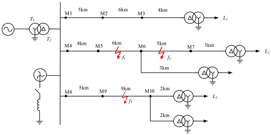
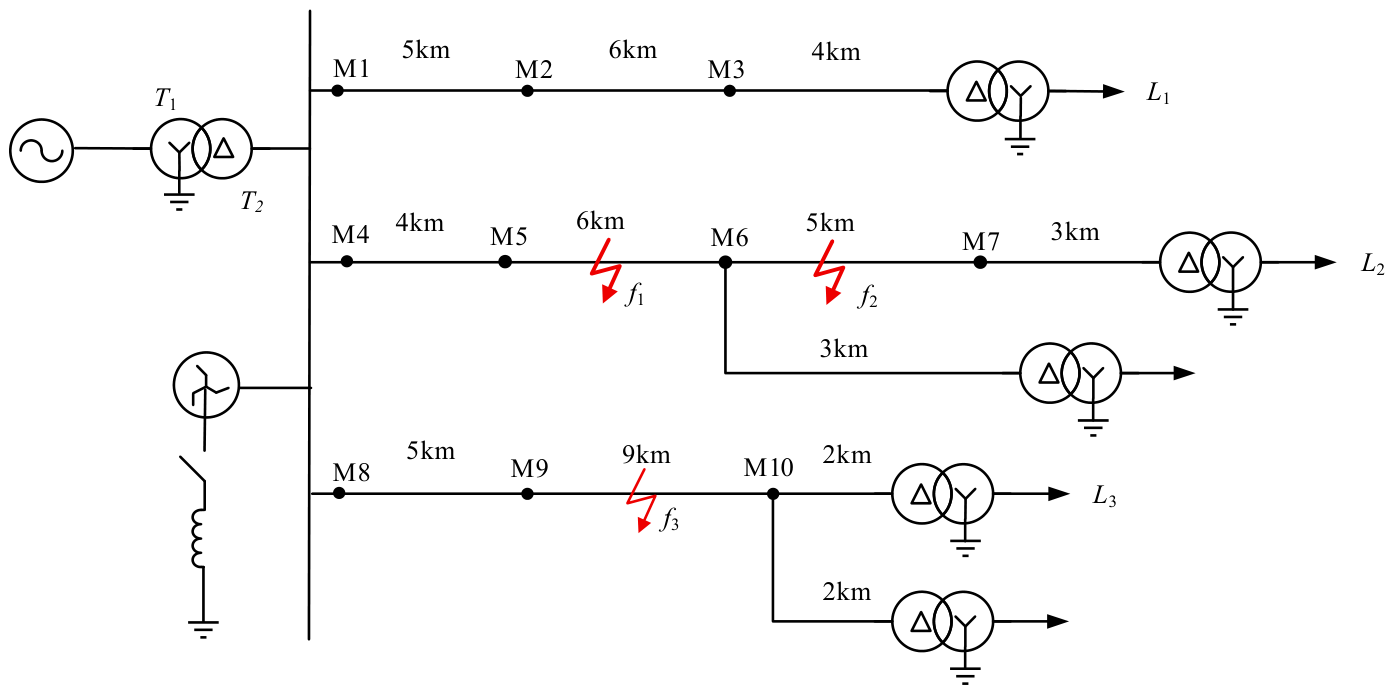
When a grounding fault occurs in this system, the fault current is usually limited to a relatively low level, generally not exceeding 10 A. Under normal operating conditions, the three-phase voltages remain balanced, and the phase-to-ground capacitive currents remain symmetrical. Under symmetrical three-phase load and line parameter conditions, no zero-sequence component exists in the system. The corresponding voltage and current phasor relationship is shown in Figure 1.

2.1.2. Fault Conditions and Data Acquisition

The simulation conditions include variations in fault distance, transition resistance, and fault inception angle. These three factors are important because they directly affect the amplitude, waveform shape, and propagation characteristics of the initial traveling wave. Fault distance changes the propagation path and arrival time difference at the two measurement terminals. Transition resistance affects the strength of the transient component, especially under high-resistance grounding conditions. The fault inception angle affects the instantaneous voltage at the fault moment and therefore changes the initial mutation amplitude of the traveling wave [18,19]. The present validation uses one PSCAD/EMTDC distribution network topology and one arc-suppression-coil grounding mode; noise realization, synchronization jitter, and other stochastic perturbations are not varied in the present data set.

The sampling frequency is set to 10 MHz, corresponding to a sampling interval of 0.1 μs. If the traveling-wave propagation velocity is approximately close to 3.0 × 10⁸ m/s, one sampling interval corresponds to an ideal one-way propagation distance interval of about 30 m. In a double-ended location calculation, the final error is also affected by the relative arrival time errors at the two terminals and by the propagation time ratio. Therefore, repeated identical error values in the following result tables should not be interpreted alone as statistical robustness; they may partly indicate that the detected wavefront arrival times fall into the same discrete sampling bins under the deterministic simulation cases. This quantization floor is considered when interpreting the results in Section 3 and Section 4. No sub-sample interpolation is employed in the present MATLAB processing; the wavefront arrival time is determined from the discrete sampling point corresponding to the first significant SDEO energy mutation. Therefore, the errors of 11–15 m should be understood as deterministic results obtained after double-ended propagation-time-ratio calculation and possible cancellation of terminal timing quantization, rather than as evidence that the method has a continuous spatial resolution below the sampling grid. The main simulation parameters and operating conditions are summarized in

Table 1. Simulation parameters and operating conditions.

Parameter	Setting
Fault type	Single-phase-to-ground fault
Grounding mode	Arc-suppression-coil-grounded system
Signal type	Three-phase voltage traveling waves at both ends of the fault section
Modal processing	Voltage line-mode component selected after Clarke transformation
Sampling frequency	10 MHz
Fault distance	1.5 km, 2.5 km, 3.5 km, 4.0 km, 6.15 km, etc.
Transition resistance	10 Ω, 100 Ω, 500 Ω, 1000 Ω
Fault inception angle	0°, 30°, 60°, 90°
Comparison methods	EMD-TEO, VMD-TEO, VMD-GST, VMD-GST-SDEO

.

2.1.3. Tested Fault Sections and Branch Boundary Condition

For the location tests in

Table 2. Location results under different fault distances and tested sections.

Fault Sequence	Fault Point	Tested Terminal Pair	Fault Distance/km	Location Result/km	Location Error/m
1	f1	M5–M6	1.5	1.455	45
2	f2	M6–M7	2.5	2.515	15
3	f2	M6–M7	3.5	3.478	22
4	f1	M5–M6	4.0	4.047	47
5	f3	M9–M10	4.0	4.026	26
6	f3	M9–M10	6.15	6.139	11

,

Table 3. Location results under different transition resistances.

Fault Point	Tested Terminal Pair	Fault Distance/km	Transition Resistance/Ω	Location Result/km	Location Error/m
f1	M5–M6	1.5	10	1.455	45
f1	M5–M6	1.5	100	1.455	45
f1	M5–M6	1.5	500	1.455	45
f1	M5–M6	1.5	1000	1.455	45
f2	M6–M7	2.5	10	2.457	43
f2	M6–M7	2.5	100	2.515	15
f2	M6–M7	2.5	500	2.515	15
f2	M6–M7	2.5	1000	2.515	15
f3	M9–M10	6.15	10	6.139	11
f3	M9–M10	6.15	100	6.139	11
f3	M9–M10	6.15	500	6.139	11
f3	M9–M10	6.15	1000	6.139	11

and

Table 4. Location errors under different fault inception angles.

Fault Point	Tested Terminal Pair	Fault Distance/km	0° Error/m	30° Error/m	60° Error/m	90° Error/m
f1	M5–M6	1.5	45	45	30	30
f2	M6–M7	2.5	23	15	15	15
f3	M9–M10	6.15	22	11	11	11

, the measuring terminals are selected at the two ends of the faulted section before the double-ended location formula is applied. The tested terminal pairs are M5–M6 for fault point f1, M6–M7 for fault point f2, and M9–M10 for fault point f3. The two 4.0 km cases in Table 2 correspond to different fault points and terminal pairs, namely f1 in M5–M6 and f3 in M9–M10, rather than duplicate calculations for the same physical case. In the tested cases, branch nodes such as M6 and M10 act as section boundary nodes rather than internal branch nodes inside the selected two-terminal measuring section. If a tested fault section contains an internal branch or a conductor-type transition, the propagation-time-ratio assumption should be corrected using a segmented model.

2.1.4. MATLAB Processing Parameters

The MATLAB processing parameters used in this study are as follows: The VMD penalty factor is set to α = 2000. The noise tolerance parameter is τ = 0. The modal number is K = 3. The DC component flag is set to 0, the initialization mode is set to 0, and the convergence tolerance is set to 1 × 10⁻⁶. These parameters are selected because K = 3 can separate the low-frequency component and the high-frequency transient component effectively in the tested cases. If K is too small, effective high-frequency information may not be fully separated. If K is too large, false components and over-decomposition may occur.

Under the fixed setting K = 3, the third/highest-frequency IMF component is retained after VMD as the high-frequency component for subsequent GST processing. GST is applied to this component to obtain a time–frequency matrix with higher time resolution in the high-frequency range. The SDEO instantaneous energy spectrum is then calculated from the selected GST-enhanced feature sequence. The first significant mutation point in the SDEO energy spectrum is used to calibrate the arrival time of the initial wavefront at each measurement terminal.

2.2. Traveling-Wave Theory for Single-Phase-to-Ground Faults

2.2.1. Generation and Propagation of Fault Traveling Waves

The transient process produced by a single-phase-to-ground fault can be considered as a superposition of the pre-fault steady-state component and the fault additional component. According to Thevenin equivalence and the superposition theorem, the sudden boundary condition change at the fault point can be represented by a virtual voltage source with the same amplitude as the pre-fault voltage and the opposite direction. This additional source generates electromagnetic waves that propagate rapidly toward both ends of the line. These waves are defined as fault traveling waves.

For theoretical analysis, line resistance and conductance per unit length are usually much smaller than line reactance and susceptance in the high-frequency transient stage. The line can therefore be approximately treated as a lossless distributed parameter line. For a differential line segment, the relationship between voltage, current, distance, and time can be described by the distributed parameter equations.

$$\left\{\begin{array}{c}-{\displaystyle \frac{\partial u(x,t)}{\partial x}}=L_0{\displaystyle \frac{\partial i(x,t)}{\partial t}}\\ -{\displaystyle \frac{\partial i(x,t)}{\partial x}}=C_0{\displaystyle \frac{\partial u(x,t)}{\partial t}}\end{array}\right.$$

(1)

In Equation (1), u(x,t) and i(x,t) denote the voltage and current at position x and time t, respectively. L₀ and C₀ denote the inductance and capacitance per unit length of the line. By eliminating voltage or current, the wave equations of voltage and current can be obtained. For the lossless line, the traveling-wave propagation velocity is expressed as follows:

$$v={\displaystyle \frac{1}{\sqrt{L_0{C}_0}}}$$

(2)

The propagation velocity is determined by the equivalent inductance and capacitance of the line. In a practical distribution network, however, the propagation process is affected by conductor arrangement, line branches, frequency-dependent parameters, and terrain conditions. These factors make the actual propagation process deviate from the ideal lossless-line model. This is one reason why direct substitution of a fixed empirical wave velocity may produce distance calculation deviation.

2.2.2. Reflection and Refraction of Traveling Waves

A practical distribution network is not an ideal infinitely long uniform line. Branch nodes, line terminals, and connection points between lines with different surge impedances are widely present. When a traveling wave reaches an impedance-discontinuous point, electromagnetic energy conservation requires the incident wave to be decomposed into a transmitted wave and a reflected wave. The transmitted wave propagates into the adjacent line, and the reflected wave propagates back along the original line. The amplitudes of the transmitted and reflected waves are related to the surge impedances on both sides of the node.

This reflection and refraction mechanism is important for distribution-network traveling-wave location because branch lines can generate multiple wavefronts after the first initial wavefront. These subsequent wavefronts may interfere with the first wavefront and make arrival time calibration difficult. Therefore, the proposed method focuses on the first significant mutation point after VMD-GST processing and uses the SDEO to identify the initial wavefront more reliably.

2.2.3. Modal Transformation and Voltage Line-Mode Component Extraction

The above theoretical analysis is based on a single-phase line model. In practical distribution lines, three-phase conductors are electromagnetically coupled. If the three-phase voltage or current traveling waves are directly processed, the coupling relationship between phases may reduce the clarity of wavefront identification. Modal transformation is therefore required to decouple the measured three-phase transient signals into independent modal components.

Common modal transformation methods include symmetrical component transformation, Karenbauer transformation, and Clarke transformation. In this study, Clarke transformation is adopted for the three-phase voltage traveling-wave signals. It transforms the measured phase-domain voltage signals into two line-mode components and one zero-mode component.

$$\left[\begin{array}{c}{u}_{\alpha }\\ u_{\beta }\\ u_0\end{array}\right]={\displaystyle \frac{2}{3}}\left[\begin{array}{ccc}1& -{\displaystyle \frac{1}{2}}& -{\displaystyle \frac{1}{2}}\\ 0& {\displaystyle \frac{\sqrt{3}}{2}}& -{\displaystyle \frac{\sqrt{3}}{2}}\\ {\displaystyle \frac{1}{2}}& {\displaystyle \frac{1}{2}}& {\displaystyle \frac{1}{2}}\end{array}\right]\left[\begin{array}{c}{u}_a\\ u_b\\ u_c\end{array}\right]$$

(3)

In Equation (3), u_a, u_b, and u_c are the three-phase voltage traveling-wave signals. u_α and u_β are the line-mode components, and u₀ is the zero-mode component. The zero-mode component is connected with the earth-return path. Its propagation velocity is affected by earth resistivity, skin effect, and frequency-dependent parameters, and it may suffer from serious attenuation and dispersion. The line-mode components propagate mainly among phases and are less affected by earth parameters. Because the current traveling wave generated under arc-suppression-coil grounding is usually weak, the voltage line-mode component is selected as the input of the proposed VMD-GST-SDEO method.

2.3. VMD-Based Decomposition of Fault Traveling Waves

2.3.1. Principle of Variational Mode Decomposition

The voltage line-mode traveling wave generated by a fault is a typical nonstationary transient signal. Its frequency components change rapidly with time. If the original signal is processed directly using a simple amplitude threshold or energy operator, high-frequency oscillation, noise, and reflected waves may cause misidentification of the initial wavefront. VMD is introduced to decompose the original line-mode component into a series of finite-bandwidth intrinsic mode functions, so that fault transient features in different frequency ranges can be separated.

VMD constructs a constrained variational problem. The input signal is decomposed into K modal components, and the sum of the estimated bandwidths of all components is minimized. Each modal component is converted into an analytic signal using Hilbert transformation. The center frequency of each modal component is shifted to the baseband through exponential demodulation, and the L2 norm of the gradient is used to estimate the bandwidth. The constrained variational problem can be written as follows [20]:

$$\left\{\begin{array}{l}\underset{\left\{u_k\right\},\left\{{\omega }_k\right\}}{\min }{\displaystyle \sum _{k=1}^K{‖{\partial }_t\left[\left(\delta \left(t\right)+\frac{j}{\pi t}\right)\ast u_k\left(t\right)\right]e^{-j{\omega }_{k}t}‖}_2^2}\hfill \\ \mathrm{s}.\mathrm{t}. {\displaystyle \sum _{k=1}^K{u}_k\left(t\right)=f\left(t\right)}\hfill \end{array}\right.$$

(4)

In Equation (4), f(t) is the input voltage line-mode traveling-wave signal, u_k(t) denotes the kth intrinsic mode function, ω_k is the corresponding center frequency, K is the number of modes, δ(t) is the impulse function, and * denotes convolution. The constrained problem is transformed into an unconstrained problem by introducing a quadratic penalty factor and a Lagrange multiplier. The alternate direction method of multipliers is then used to update the modal components, center frequencies, and multipliers iteratively until the convergence condition is satisfied.

2.3.2. Parameter Setting and High-Frequency Mode Selection

The decomposition performance of VMD depends strongly on the penalty factor and the number of modes. The penalty factor controls the bandwidth of each intrinsic mode function. If the value is too small, each component has a wide bandwidth, and different frequency components may mix with each other. If the value is too large, local mutation information may be excessively smoothed, which is not beneficial for extracting high-frequency fault-transient features. In the original algorithm, the penalty factor is set to 2000, which lies in the common range used for feature extraction.

The mode number K determines how many components the original signal is decomposed into. If K is too small, the effective high-frequency transient component may not be separated sufficiently. If K is too large, over-decomposition and false components may occur. Based on the original frequency spectrum characteristics and decomposition effect, K = 3 is selected. Under this setting, the low-frequency background component and the high-frequency fault-transient component can be distinguished more clearly. Under the fixed setting K = 3, the third/highest-frequency IMF component is retained by construction for GST processing, rather than being selected through an additional data-dependent comparison step.

Compared with EMD, VMD provides a clearer bandwidth constraint and can reduce mode mixing and end effects to a certain extent. This feature is important for fault traveling waves because the initial wavefront is short and easily covered by oscillation or reflection. By using VMD before GST and the SDEO, the proposed method improves the stability of wavefront feature extraction.

2.3.3. Necessity of VMD for Traveling-Wave Preprocessing

The decomposition behavior of different signal-processing methods was compared to explain the selection of VMD. EMD decomposes a signal adaptively, but it easily produces mode mixing and end effects when the input signal contains a strong transient mutation and multiple frequency components. For traveling-wave signals in distribution networks, this problem is especially important because the initial wavefront may be mixed with reflected waves and oscillatory components. If the decomposition result cannot isolate the high-frequency mutation clearly, the subsequent energy-operator stage may lock onto a secondary oscillation instead of the first wavefront.

CEEMDAN can reduce some problems of EMD by adding adaptive noise and ensemble averaging. However, residual noise, false components, and mode mixing may still appear when complicated fault-transient signals are decomposed. For a fault location method, these false components are not just a signal-processing problem; they may also produce a direct distance error because the final location formula depends on the calibrated arrival times. A small arrival time deviation can be amplified into a location deviation after distance calculation.

VMD is therefore used as the preprocessing stage in this method. Unlike EMD, VMD decomposes the signal through a variational framework with a clear bandwidth constraint. The decomposition is solved in the frequency domain, and each modal component has a corresponding center frequency. This makes the high-frequency transient component easier to identify. Under the parameter setting K = 3 and α = 2000, the original method obtains a relatively clear separation between low-frequency components and the high-frequency mutation component. This provides a more reliable foundation for GST and SDEO processing.

2.4. GST-SDEO Initial Wavefront Calibration

2.4.1. Generalized S-Transform

The S-transform is a time–frequency analysis method that combines the advantages of the short-time Fourier transform and continuous wavelet transform. It introduces a frequency-dependent Gaussian window and generates a time–frequency matrix. The matrix can describe the instantaneous amplitude distribution of different frequency components. For a nonstationary fault traveling-wave signal, this time–frequency representation is useful for identifying local mutation features near the initial wavefront.

The conventional S-transform uses a fixed relationship between window width and frequency. When processing complicated distribution-network traveling waves, a fixed window may not provide sufficient adaptability for different frequency ranges. The generalized S-transform introduces a window adjustment parameter, allowing the Gaussian window width to change with frequency more flexibly. When the adjustment parameter is larger than one, higher time resolution can be obtained in the high-frequency range, which is suitable for highlighting the initial traveling-wave mutation [21].

$$GST(\tau ,f)={\displaystyle {\int }_{-\infty }^{+\infty }s(t)\frac{{\left|f\right|}^p}{\sqrt{2\pi }}}\cdot e^{-{\displaystyle \frac{{(\tau -t)}^2{f}^{2p}}{2}}}\cdot e^{-j2\pi ft}dt$$

(5)

In Equation (5), s(t) is the IMF component to be analyzed, τ is the time-shift factor, f is the frequency, and p is the window adjustment parameter. After GST is applied to the selected high-frequency IMF component, a time–frequency energy matrix with high time resolution near the initial wavefront is obtained. This matrix enhances the local mutation feature and provides a clearer input for SDEO energy analysis.

2.4.2. Symmetric Difference Energy Operator

The Teager energy operator can track instantaneous amplitude and frequency variation with low computational complexity. However, the operator may produce asymmetric response error at mutation points and is sensitive to noise. The symmetric difference energy operator is derived by introducing a central finite-difference structure [22]. This structure smooths the discrete signal and improves the stability of mutation point tracking.

Let z(n) be the energy feature sequence obtained after GST processing, and let T_s be the sampling period. The first-order and second-order central differences can be expressed as follows:

$$\left\{\begin{array}{c}{z}^{\prime }(n)={\displaystyle \frac{z(n+1)-z(n-1)}{2T_s}},\\ z^{″}(n)={\displaystyle \frac{z(n+1)-2z(n)+z(m-1)}{T_s^2}}.\end{array}\right.$$

(6)

Based on the above difference forms, the SDEO instantaneous energy spectrum is defined as:

$${\psi }_{SDEO}(n)={\left[z^{\prime }(n)\right]}^2-z(n)z^{″}(n)$$

(7)

When the initial traveling wave arrives at a measurement point, both amplitude and frequency components of the signal change abruptly. Equation (7) is sensitive to this type of mutation. The first significant mutation point in the SDEO energy spectrum is therefore selected as the arrival time of the initial wavefront. Compared with direct mutation point detection from the original waveform, this processing avoids misidentification caused by oscillation and reflected waves. Compared with a single TEO or a single GST method, the VMD-GST-SDEO combination provides more stable wavefront calibration for weak mutation conditions.

2.4.3. Wavefront Calibration Procedure

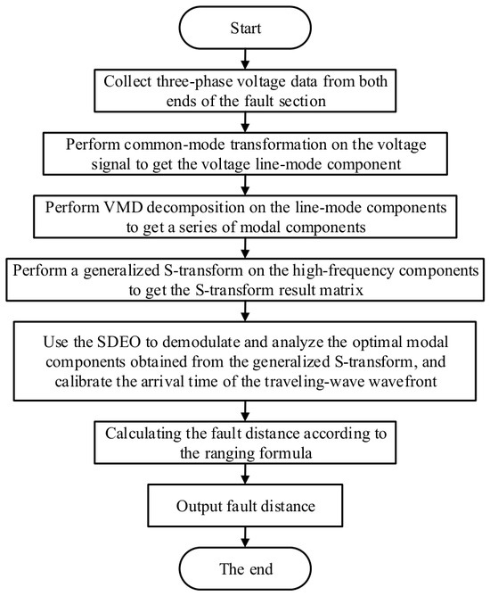
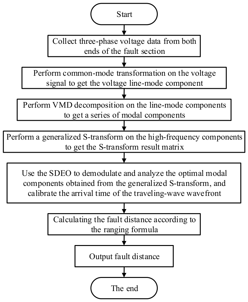
The wavefront calibration process includes four steps. First, the three-phase voltage traveling waves measured at both ends of the fault section are transformed using Clarke transformation, and the voltage line-mode component is obtained. Second, VMD is applied to the line-mode component, and the high-frequency IMF component containing the fault mutation feature is selected. Third, GST is used to obtain the local time–frequency distribution of the high-frequency component. Fourth, the SDEO instantaneous energy spectrum is calculated, and the first significant energy mutation point is used to determine the wavefront arrival time at each terminal.

The overall procedure of the proposed method is shown in Figure 2. The flowchart includes data acquisition, modal transformation, VMD decomposition, GST time–frequency analysis, SDEO mutation point detection, and improved double-ended distance calculation.

2.4.4. Role of SDEO in Weak Mutation Wavefront Identification

The initial traveling-wave wavefront may be weak when the fault inception angle is small or when the transition resistance is high. In this situation, direct peak detection from the original line-mode waveform is not stable because the first mutation may not be the largest point in the waveform. Later reflected waves or oscillatory components may have larger amplitudes than the first arrival. If the arrival time is determined only by amplitude comparison, the method may select a later wavefront and introduce an error into the distance calculation.

The SDEO stage is used to avoid this problem by focusing on the energy mutation rather than the raw amplitude. The center-difference structure of the SDEO uses adjacent sampling points to describe the instantaneous change of the signal. When the first traveling wave arrives, the waveform slope and local frequency content both change quickly. This change appears as a sharp point in the SDEO energy spectrum. Because GST has already enhanced the local time–frequency features, the SDEO output can indicate the first mutation more clearly.

This processing chain also explains why the proposed method performs better than methods using only one or two stages. VMD alone can separate frequency components but cannot determine the arrival time. GST alone can show time–frequency energy concentration but may still require threshold judgment. The SDEO alone may be affected by noise and raw waveform oscillation. The combined process uses each step for a specific function: VMD separates modes, GST enhances time–frequency features, and the SDEO detects the first energy mutation.

2.5. Improved Double-Ended Traveling-Wave Location Model

2.5.1. Conventional Double-Ended Traveling-Wave Location Formula

The conventional double-ended traveling-wave method uses the time difference between the arrival times of the initial wavefront at both ends of the line. Suppose that the horizontal length of the fault section is L, the fault point is located at a distance x_s from the upstream terminal, and the initial traveling wave reaches the upstream and downstream terminals at times t_m and t_n, respectively. The conventional formula can be written as follows:

$$x_s={\displaystyle \frac{L+v(t_m-t_n)}{2}}$$

(8)

Equation (8) requires a predefined traveling-wave velocity v. In practical distribution lines, v is affected by line parameters, conductor arrangement, frequency dispersion, and environmental conditions. If an empirical velocity is directly used, the location result may deviate from the actual fault position. Moreover, the actual conductor length may differ from the horizontal length because of terrain and sag. These factors reduce the stability of the conventional location formula.

2.5.2. Improved Propagation-Time-Ratio Formula

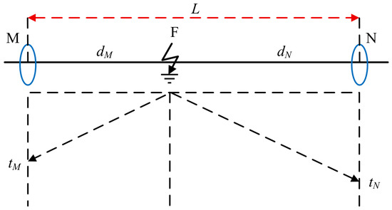
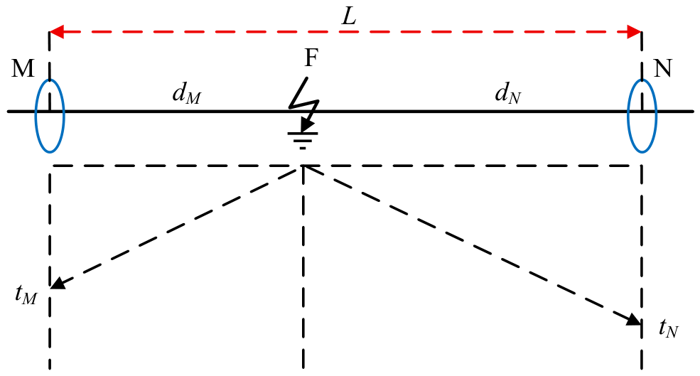
To reduce the dependence on fixed empirical velocity, this study introduces a double-ended absolute propagation-time-ratio model. Let T_m and T_n denote the absolute propagation times from the fault point to the upstream and downstream terminals, respectively. If the conductors and propagation environment in the same fault section are approximately consistent, the traveling-wave velocities on both sides of the fault point can be considered identical or nearly identical. Under this condition, the ratio of the horizontal distance from the fault point to one terminal to the section horizontal length is approximately equal to the ratio of the corresponding propagation time to the total propagation time.

$${\displaystyle \frac{x}{L}}={\displaystyle \frac{T_m}{T_m+T_n}}$$

(9)

The improved double-ended location formula can therefore be written as:

$$x={\displaystyle \frac{L{T}_m}{T_m+T_n}}$$

(10)

In Equation (10), x is the horizontal distance from the upstream terminal to the fault point, and L is the horizontal length of the fault section. Compared with Equation (8), Equation (10) does not explicitly introduce a fixed empirical wave velocity. It calculates the fault position according to the propagation time ratio at both ends. This formulation reduces the influence of wave-velocity selection and actual line length deviation on the location result. The principle of the improved double-ended location model is shown in Figure 3.

The absolute propagation times T_m and T_n are obtained from the time interval between the fault inception reference and the calibrated arrival time of the initial wavefront at the two terminals. In the PSCAD/EMTDC simulation, the fault inception time is known from the preset fault trigger, so T_m and T_n can be extracted directly from the simulated waveform window. In practical implementation, the fault inception reference should be obtained from a high-speed disturbance trigger, such as a zero-sequence-voltage mutation trigger or a common GPS/BeiDou-synchronized recording trigger. Therefore, the improved formula still requires accurate triggering and terminal synchronization, although it avoids direct substitution of a fixed empirical wave velocity.

To clarify the influence of timing errors, let the measured propagation time errors at the upstream and downstream terminals be ΔT_m and ΔT_n, respectively. For Equation (10), the first-order location error perturbation can be written as follows:

$$\Delta x\approx {\displaystyle \frac{L(T_n\Delta T_m-T_m\Delta T_n)}{{(T_m+T_n)}^2}}$$

(11)

This expression shows that independent timing errors at the two terminals directly affect the calculated distance. If both terminal records are shifted by the same common time offset, the error is partly canceled in the ratio form; however, a relative synchronization error between the two terminals is still converted into a location error. Using the propagation velocity approximation v = 3.0 × 10⁸ m/s for order-of-magnitude estimation, a relative terminal timing error of 0.1 μs corresponds to an equivalent double-ended distance error of approximately vΔt/2, namely about 15 m. Thus, the reported 11–15 m errors are already close to the timing-quantization floor of the 10 MHz sampling setting. This point is considered when interpreting the simulation results, and the method should not be described as having sub-sample accuracy unless interpolation or higher-frequency sampling is further introduced.

2.5.3. Fault Location Procedure

The accurate fault location procedure can be summarized as follows: First, after the fault section is determined, voltage traveling-wave recording devices at both ends of the fault section collect the post-fault three-phase voltage signals. Second, Clarke transformation is performed to obtain the voltage line-mode component. Third, VMD is used to decompose the line-mode component into several IMF components, and, under K = 3, the third/highest-frequency IMF component is retained as the high-frequency component related to the initial traveling wave. Fourth, GST is applied to the high-frequency IMF component to enhance the local time–frequency mutation feature. Fifth, the SDEO is used to calculate the instantaneous energy spectrum, and the first significant mutation point is taken as the initial wavefront arrival time. Finally, the improved double-ended location formula is used to calculate the fault distance.

This method combines signal preprocessing, time–frequency enhancement, energy mutation detection, and double-ended location model improvement. The method is especially suitable for the condition in which the fault current is weak but the voltage traveling wave contains identifiable high-frequency transient information.

2.6. Algorithm Implementation and Reproducibility Description

2.6.1. Input Data Organization

The MATLAB program reads the voltage traveling-wave data exported from the PSCAD/EMTDC model and then performs signal processing in sequence. The data file contains the sampled three-phase voltage signals at the measurement terminals. For each fault condition, the program first determines the time window around the fault inception moment and extracts the corresponding voltage samples. This window contains the initial wavefront and several later oscillatory components. The subsequent algorithm uses this window rather than the entire steady-state waveform, which reduces unnecessary computation and focuses the analysis on the transient stage that contains location information.

The 10 MHz sampling condition is used consistently for all deterministic cases. No sub-sample interpolation is used in the MATLAB processing, and the arrival time is selected according to the discrete SDEO mutation point. Therefore, the reported deterministic location errors should be interpreted together with the timing-quantization floor of the sampling setting, rather than as evidence of continuous sub-sample spatial resolution.

2.6.2. Signal Processing Sequence

The MATLAB implementation follows the theoretical procedure described above. The three-phase voltage signals are first transformed into modal quantities using Clarke transformation. The line-mode voltage component is selected because it has a more stable propagation path than the zero-mode component. The selected line-mode signal is then decomposed using VMD. The algorithm parameters are set as K = 3 and α = 2000. Under this fixed K value, the third IMF component corresponds to the highest-frequency mode in the adopted decomposition order and is retained by construction for subsequent GST processing, rather than being selected through a data-dependent visual comparison among candidate IMFs.

After GST processing, the time–frequency matrix is converted into an energy feature sequence. This sequence is smoother and more concentrated around the initial wavefront than the original voltage waveform. The SDEO is then applied to the sequence, and the first significant energy mutation is used as the wavefront arrival time. The same operation is performed for the two terminals of the fault section. The two arrival times are converted into the absolute propagation times Tm and Tn used in the improved location formula.

For reproducibility, the arrival time calibration rule used in the MATLAB implementation can be summarized as follows: Step 1: Use a preset fault inception reference to define a short analysis window around the transient stage. Step 2: Extract the voltage line-mode signal at the two terminals and decompose it using VMD with K = 3 and α = 2000. Step 3: Retain the third/highest-frequency IMF component by construction as the high-frequency component containing the initial traveling-wave mutation under K = 3. Step 4: Apply GST to the selected IMF and take the high-frequency row of the GST magnitude matrix as the feature sequence. Step 5: Remove the edge-affected samples by using a safe index window. Step 6: Calculate the absolute SDEO sequence of the GST feature. Step 7: Within the post-fault search interval from tfault + 2 μs to tfault + 100 μs, select the sample with the maximum SDEO response as the first significant mutation point. Step 8: Convert the two selected sample times into Tm and Tn and substitute them into the improved double-ended formula. This rule explains that the present implementation uses a discrete peak-search criterion in a predefined post-fault window rather than sub-sample interpolation or a statistically optimized adaptive threshold.

2.6.3. Parameter-Sensitivity Discussion

The wavefront calibration result is affected by the VMD penalty factor, VMD modal number, GST window adjustment parameter, SDEO mutation criterion, and high-frequency IMF selection rule. In this study, these parameters are fixed according to the MATLAB processing implementation and deterministic simulation cases. A complete numerical sweep over all parameter combinations is not included because the available validation set does not contain the additional waveform data required for statistically meaningful parameter sensitivity analysis.

For VMD, the modal number K determines whether the transient high-frequency component can be separated from the low-frequency background. If K is too small, the fault mutation may remain mixed with the background component. If K is too large, over-decomposition and false modes may appear. The penalty factor α controls modal bandwidth. A smaller α may cause mode mixing, whereas an excessively large α may smooth local mutation features and weaken wavefront identification. The settings K = 3 and α = 2000 are therefore used as fixed parameters for the present deterministic validation.

For GST, the window adjustment parameter controls the tradeoff between time and frequency resolution. A wider high-frequency window may blur the mutation time, while an overly narrow window may increase sensitivity to noise. For the SDEO, the mutation criterion determines which energy change is selected as the first wavefront. A low threshold may select a noise-induced fluctuation, whereas a high threshold may skip the first weak mutation and select a later reflected wave. In this study, the first significant SDEO energy mutation after VMD-GST preprocessing is selected consistently for the two terminals.

The high-frequency IMF selection rule is also important. The selected IMF should contain the first traveling-wave mutation and should not be dominated by low-frequency background variation or later reflected-wave components. If multiple high-frequency IMFs contain comparable mutation features, cross-checking the first SDEO mutation time among candidate IMFs is recommended. In future work, quantitative parameter-sensitivity analysis should be carried out by sweeping K, α, the GST window parameter, SDEO threshold settings, sampling frequency, and noise level using repeated stochastic simulations and field-measured traveling-wave records.

2.6.4. Distance Calculation and Error Evaluation

After the arrival times at both terminals are obtained, the improved double-ended formula is used to calculate the fault distance. The fault section horizontal length is taken from the simulation model. The calculated distance is compared with the known fault distance set in PSCAD/EMTDC. The absolute error is defined as the absolute difference between the calculated location and the actual location multiplied by 1000, with the final unit expressed in meters.

The same error definition is used in all result tables, including the fault distance test, transition resistance test, fault inception angle test, and comparison with other wavefront calibration methods. No repeated-trial statistic or confidence interval is reported because the available validation set consists of deterministic PSCAD/EMTDC-MATLAB simulation cases. Therefore, the reported errors are point estimates for the studied conditions, and the manuscript avoids treating them as statistical robustness indicators.

$$\epsilon =\left|x-x_0\right|\times 1000$$

(12)

In this expression, x₀ is the actual fault distance in kilometers, x is the calculated fault distance in kilometers, and ε is the absolute location error in meters. The smaller the value of ε, the closer the calculated location is to the actual fault position.

3. Results

3.1. Representative Case Analysis

3.1.1. Line-Mode Voltage and High-Frequency IMF Components

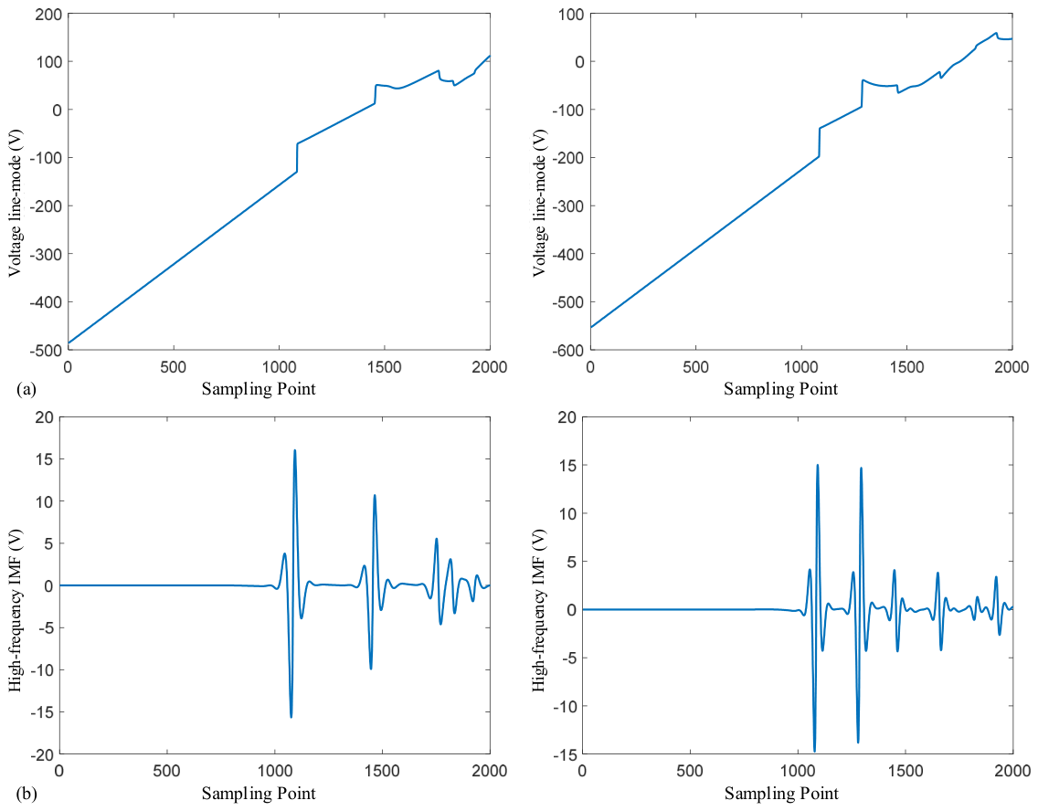
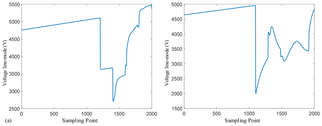
A representative case is selected to illustrate the proposed wavefront calibration process. The fault distance is 2.5 km, the transition resistance is 100 Ω, and the fault inception angle is 30°. The three-phase voltage signals measured at both ends of the fault section are transformed using Clarke transformation, and the voltage line-mode component is extracted. After the fault occurs, the line-mode component contains a step-like mutation and high-frequency oscillation near the initial wavefront arrival time. However, the mutation duration is short, and direct manual identification from the original waveform is unstable.

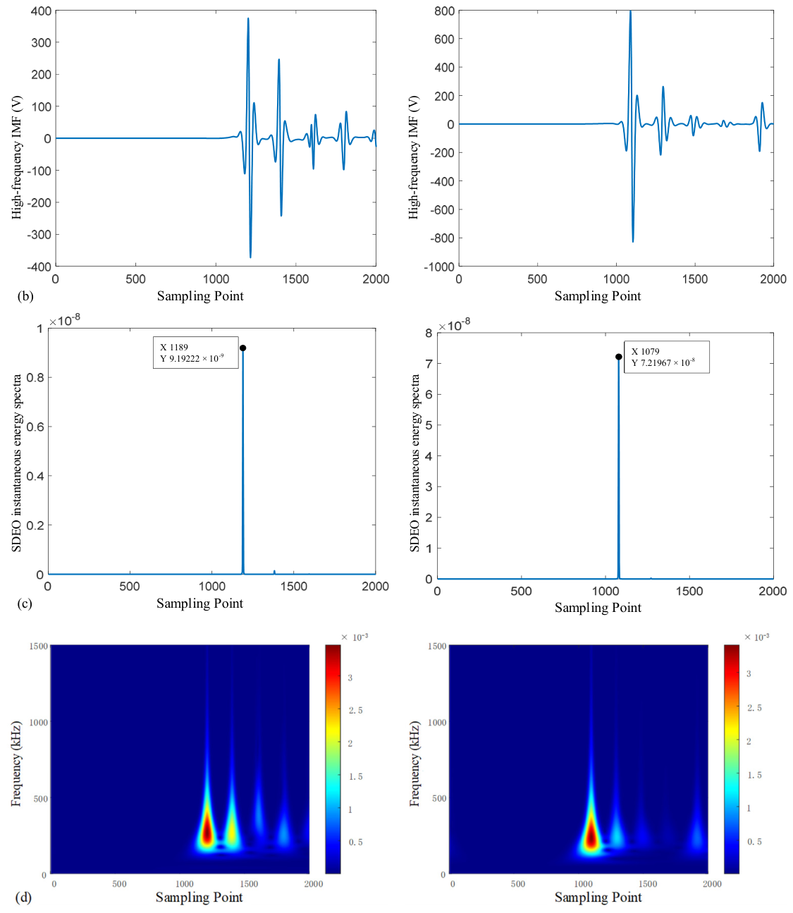
After VMD decomposition, the high-frequency IMF component more clearly represents the initial wavefront mutation information. The low-frequency trend and part of the background oscillation are separated into other modal components. This decomposition provides a more suitable input signal for the subsequent GST-SDEO processing.

3.1.2. GST Enhancement and SDEO Energy Spectrum

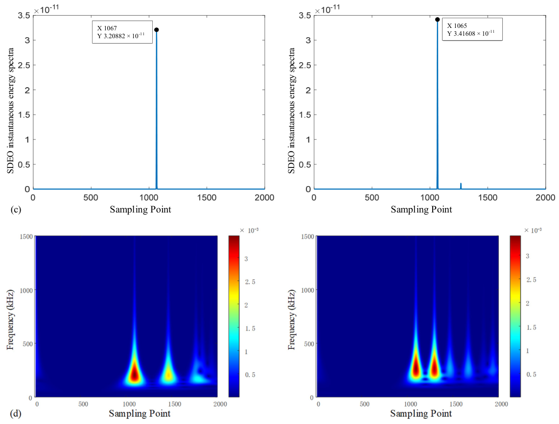
The high-frequency IMF component is further processed using GST. The time–frequency diagram shows that the energy distribution is concentrated near the wavefront arrival time. After SDEO energy demodulation, the first significant mutation point in the energy spectrum becomes clear. These mutation points at the two terminals are used to calculate the absolute propagation times.

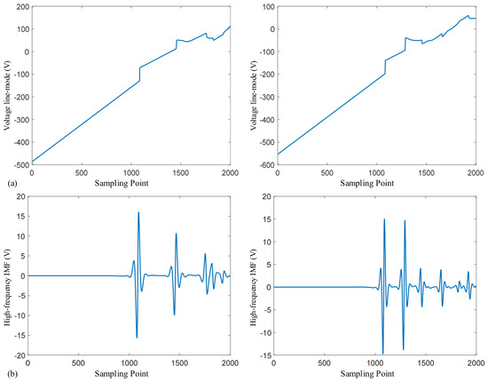
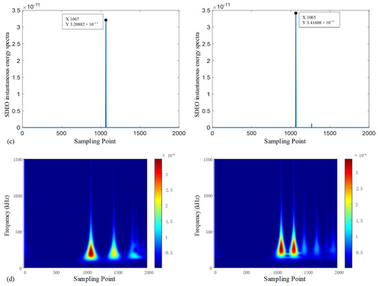
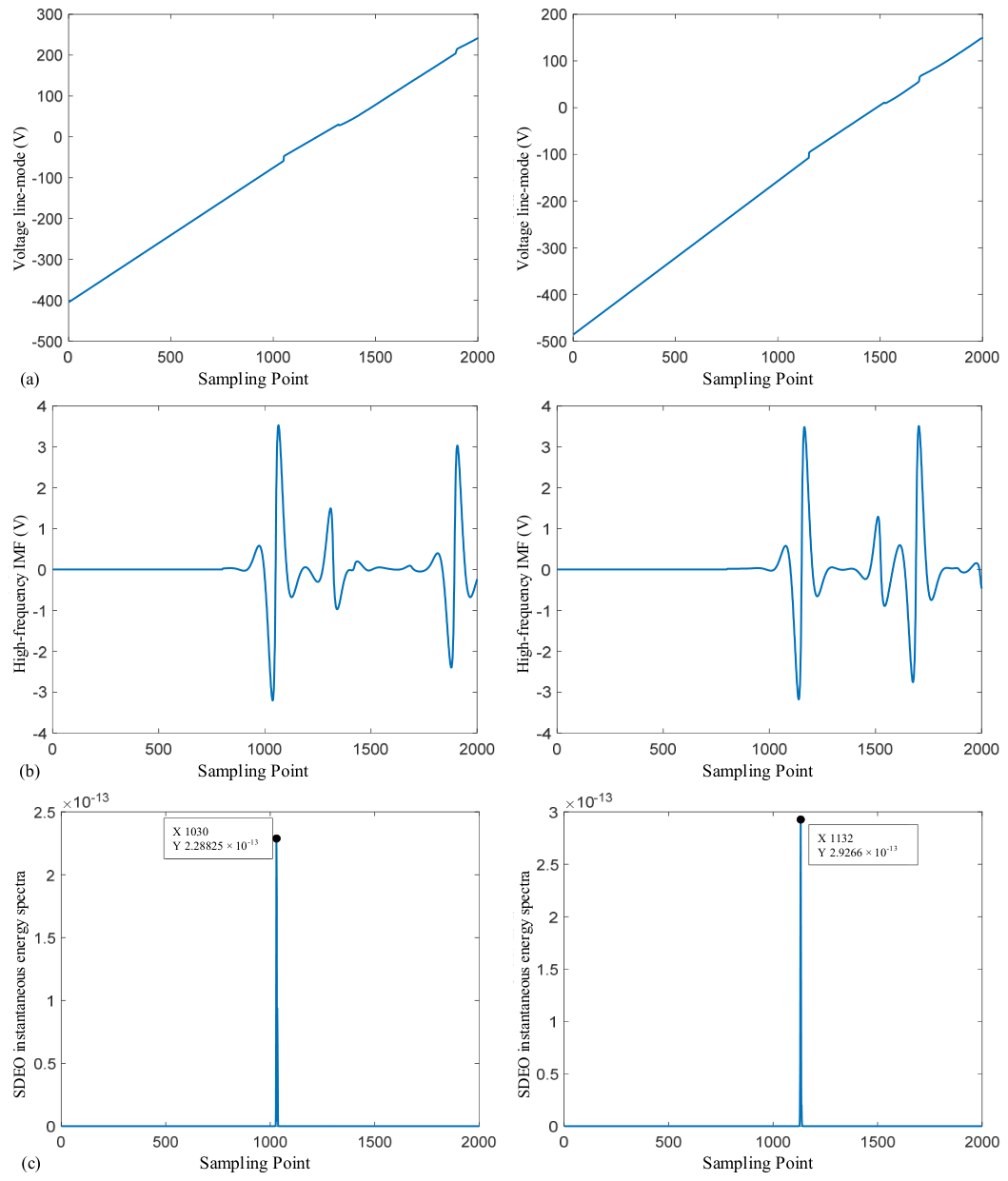
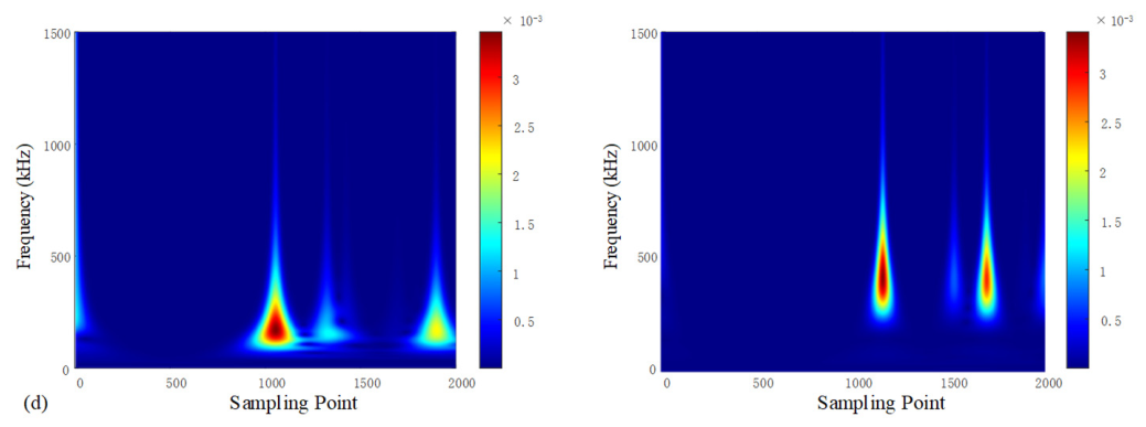
Figure 4 presents the representative simulation results, including the voltage line-mode components at both ends of the fault section, the selected high-frequency IMF components, the GST time–frequency diagrams, and the SDEO instantaneous energy spectra. According to the mutation points in the SDEO spectra, the calculated fault location is 2.515 km. The absolute location error is 15 m. This result indicates that the VMD-GST-SDEO framework can extract a stable wavefront feature from the nonstationary fault transient signal.

3.2. Adaptability Under Different Fault Distances

Fault distance changes the traveling-wave propagation path and the arrival time difference at both terminals. To verify the adaptability of the proposed method to fault position variation, single-phase-to-ground faults are set at several different positions. The transition resistance is 100 Ω, and the fault inception angle is 30°. The location results are listed in Table 2. The two 4.0 km entries correspond to different fault points and terminal pairs, and the results are therefore grouped by fault point and tested terminal pair.

The results show that the absolute location error remains below 100 m when the tested fault distance varies from 1.5 km to 6.15 km. The minimum error is 11 m, and the maximum error is 47 m. The results indicate that the proposed VMD-GST-SDEO calibration and the propagation-time-ratio formula can provide correct deterministic location results for the studied cases. Because the sampling interval is 0.1 μs, the error values should also be interpreted together with the sampling-bin resolution discussed in Section 2.1.2.

3.3. Adaptability Under Different Transition Resistances

3.3.1. Location Results Under Transition-Resistance Variation

Transition resistance directly affects the transient amplitude at the fault point. A larger transition resistance weakens the fault transient component and makes the initial wavefront mutation less pronounced. To verify the resistance adaptability of the proposed method, faults are set at 1.5 km, 2.5 km, and 6.15 km. The fault inception angle is 30°, and the transition resistance is set to 10 Ω, 100 Ω, 500 Ω, and 1000 Ω. The results are shown in Table 3.

The results indicate that the proposed method maintains an absolute location error of less than 100 m over the transition-resistance range from 10 Ω to 1000 Ω. At the 1.5 km fault point, the error remains 45 m for all tested transition resistances. At the 2.5 km fault point, the error is 43 m under 10 Ω and 15 m under 100 Ω, 500 Ω, and 1000 Ω. At the 6.15 km fault point, the error remains 11 m under all tested transition resistances. These repeated values indicate that the identified wavefronts may fall into the same discrete sampling bins under these deterministic cases; therefore, they should be interpreted as deterministic consistency within the current sampling resolution rather than as repeated-trial statistical robustness.

3.3.2. High-Transition-Resistance Waveform Analysis

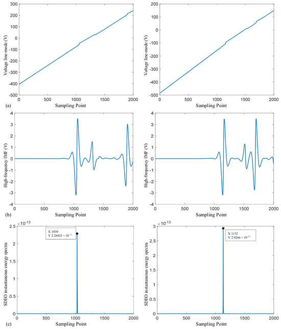
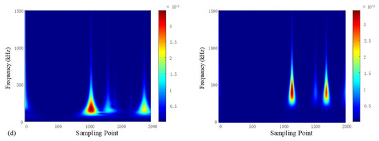
A 500 Ω transition-resistance fault is selected as a typical high-resistance condition. Although the transient amplitude is weakened by the high transition resistance, the line-mode component still contains the initial mutation feature. After VMD decomposition, the high-frequency IMF component preserves the mutation information more clearly than the original waveform. GST further enhances the local time–frequency feature, and the SDEO identifies the first energy mutation point.

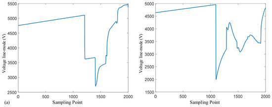
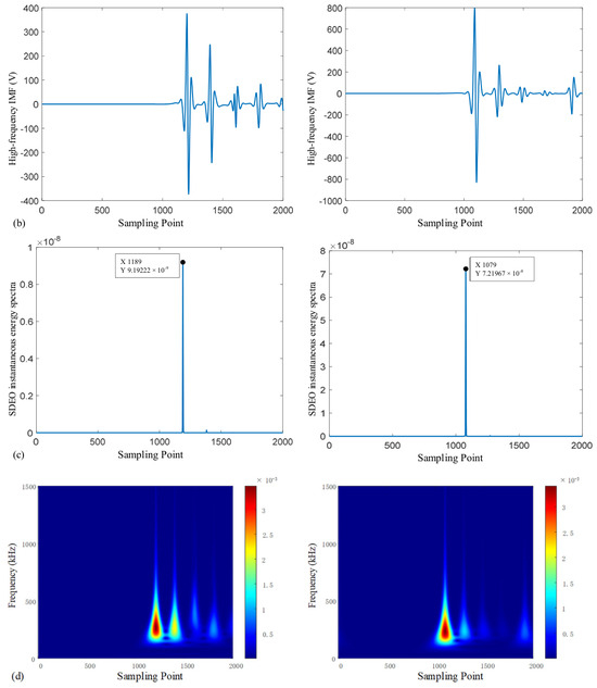
Figure 5 shows the simulation results under the 500 Ω transition-resistance fault. The results demonstrate that the first energy mutation point can still be identified after time–frequency enhancement and energy demodulation. The calculated location result is 1.455 km, and the absolute location error is 45 m.

3.4. Adaptability Under Different Fault Inception Angles

3.4.1. Location Error Under Different Inception Angles

The fault inception angle affects the instantaneous voltage at the fault moment and therefore changes the amplitude and mutation strength of the fault transient. When the inception angle is small, the transient mutation may be weak, which increases the difficulty of wavefront identification. To verify the influence of this factor, the transition resistance is set to 100 Ω, and fault inception angles of 0°, 30°, 60°, and 90° are tested. The results are listed in Table 4.

The errors at the three tested fault positions remain within the range of 11–45 m. Even under a 0° fault inception angle, the proposed method maintains stable location results in the deterministic simulation cases. This demonstrates that GST-SDEO has a certain capability for identifying weak mutation wavefronts under the tested simulation conditions.

3.4.2. Typical 60° Inception Angle Result

A representative 60° fault inception angle case is further analyzed. The fault point is f3 in the M9–M10 section, the fault distance is 6.15 km, and the transition resistance is 100 Ω. Under this condition, the voltage line-mode component presents an obvious mutation. The high-frequency IMF component and GST time–frequency diagram highlight the initial wavefront region, and the SDEO energy spectrum provides a clear mutation point. The corresponding error value in Table 4 is 11 m.

Figure 6 shows the simulation results under the 60° fault inception angle. The calibrated SDEO mutation points correspond to the arrival times used in the improved double-ended distance calculation.

3.5. Comparison with Different Wavefront Calibration Methods

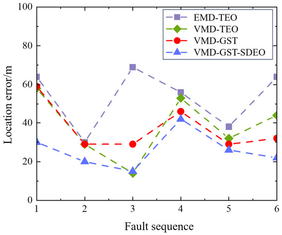
To further verify the effectiveness of the proposed VMD-GST-SDEO wavefront calibration strategy, EMD-TEO, VMD-TEO, VMD-GST, and the proposed method are compared under six fault positions. EMD-TEO can use the energy operator to detect mutation points, but EMD is prone to mode mixing and end effects when processing transient traveling waves. The separation of high-frequency features is not sufficiently stable, leading to larger location errors. VMD-TEO improves the signal decomposition quality by using VMD, but a single TEO is still sensitive to weak wavefronts and noise. VMD-GST enhances local time–frequency features, but without subsequent energy mutation detection, wavefront calibration can still be influenced by threshold selection.

The proposed VMD-GST-SDEO method combines narrowband decomposition, time–frequency enhancement, and mutation detection. The comparison results show that EMD-TEO has a maximum location error of 69 m and a minimum error of 30 m. VMD-TEO and VMD-GST improve location accuracy to some extent, but their overall errors remain higher than those of VMD-GST-SDEO. The average error of the proposed method at six different fault positions is approximately 26 m. Figure 7 shows the location error comparison of different methods.

4. Discussion

4.1. Mechanism-Level Advantages of VMD-GST-SDEO

The advantage of the proposed method comes from the cooperation of the three signal-processing stages. VMD first decomposes the original voltage line-mode traveling wave into several finite-bandwidth IMF components. This decomposition separates the high-frequency mutation component from low-frequency background variation and reduces the probability of direct misidentification from the original waveform. GST then enhances local time–frequency features of the selected high-frequency mode. Because the initial wavefront is a short-duration mutation, a time–frequency representation with high time resolution is useful for wavefront calibration. Finally, the SDEO uses a central difference structure to extract the energy mutation point. This operation is more stable than direct amplitude thresholding under weak mutation conditions.

The method therefore uses physical characteristics and signal-processing characteristics simultaneously. The input signal is a voltage line-mode traveling wave, which is relatively stable compared with the zero-mode component. The wavefront is calibrated using local mutation information rather than steady-state amplitude variation. This feature makes the method suitable for small-current grounding systems, in which steady-state current features may be weak or affected by arc-suppression-coil compensation.

4.2. Interpretation of the Improved Double-Ended Location Formula

In a conventional double-ended traveling-wave formula, the wave velocity is an explicit input. Once the selected velocity deviates from the actual propagation velocity, the calculated fault position is affected. The improved formula in this study uses the absolute propagation time ratio. When the propagation velocity on both sides of the fault point is approximately the same within the same fault section, the ratio of horizontal distance can be represented by the ratio of propagation time. Therefore, the final formula depends on the section horizontal length and the two absolute propagation times instead of depending directly on an empirical velocity.

The improved formula also has clear sensitivity to wavefront timing errors. As shown by Equation (11), independent timing errors at the two terminals, including synchronization error, ADC sampling quantization, and channel noise, can perturb both the numerator and the denominator of the propagation time ratio. The 10 MHz sampling rate gives a 0.1 μs sampling interval, corresponding to an ideal propagation distance interval of about 30 m. This explains why several deterministic cases show repeated or close error values: the identified arrival time can fall into the same sampling bin under different operating conditions.

This improvement is meaningful for reducing the explicit dependence on a selected empirical wave velocity, but it does not eliminate the requirement for accurate time synchronization. If a common time offset affects both terminal records equally, its influence can be partly canceled in the ratio. However, the relative clock error between the two terminals changes Tm and Tn differently and may directly affect the calculated distance. Therefore, the proposed formula should be used together with high-precision synchronized acquisition devices. Quantitative tests with controlled synchronization error, jitter, and measurement noise will be necessary in future work to fully evaluate engineering robustness.

The propagation-time-ratio formula is most appropriate when the selected fault section can be treated as a section with approximately uniform propagation characteristics. In mixed overhead cable sections, sections containing conductor-type transitions, or feeders with an internal branch between the two measurement terminals, the propagation velocity and wave attenuation on the two sides of the fault point may differ. Under these conditions, the simple ratio model may introduce systematic error, and a segmented propagation model or calibrated section-specific velocity ratio should be used. Because the available validation data do not include mixed overhead cable or nonuniform parameter cases, this limitation is now stated explicitly rather than treated as already verified.

4.3. Interpretation of the Existing Simulation Results

The deterministic simulation results show that the proposed method maintains errors below 100 m under the studied changes in fault distance, transition resistance, and fault inception angle. The fault distance results indicate that the method can calculate the fault position correctly for the selected tested sections. The transition-resistance results indicate that the wavefront can still be calibrated under high transition resistance after VMD-GST-SDEO processing. The inception angle results show that weak mutation conditions can also be handled within the adopted sampling resolution. However, because the validation set does not include repeated trials, noise realizations, synchronization jitter tests, or confidence intervals, these results should be understood as deterministic simulation evidence rather than full statistical robustness verification.

The comparison with EMD-TEO, VMD-TEO, and VMD-GST further explains the role of each processing stage. EMD-TEO suffers from mode mixing during decomposition. VMD-TEO improves decomposition but still relies on a single energy operator. VMD-GST enhances the time–frequency representation but does not include the SDEO mutation detection step. The proposed method integrates the advantages of these stages and therefore obtains lower and more stable location errors under the deterministic test conditions listed in

Table 5. Error values underlying Figure 7 for different wavefront calibration methods.

Fault Sequence	Fault Point	Fault Distance/km	Tested Terminal Pair	EMD-TEO Error/m	VMD-TEO Error/m	VMD-GST Error/m	VMD-GST-SDEO Error/m
1	f1	1.5	M5–M6	64	58	56	45
2	f2	2.5	M6–M7	30	29	29	15
3	f2	3.5	M6–M7	69	14	30	22
4	f1	4.0	M5–M6	56	53	46	47
5	f3	4.0	M9–M10	38	32	29	26
6	f3	6.15	M9–M10	64	44	32	11

.

The comparison is limited to EMD-TEO, VMD-TEO, and VMD-GST because the available data set contains only the deterministic waveforms and error values used for these algorithms. Recent wavelet-based, Hough-transform, threshold-free, and intelligent fault location methods are important reference methods, but a fair numerical comparison would require implementing each method under the same topology, sampling frequency, noise condition, and terminal configuration. Since such additional simulations are not available in the present data set, this manuscript does not create unsupported comparison values and instead lists broader comparative evaluation as future work.

The result groups are interpreted according to the revised tables and figures. The fault distance, transition resistance, fault inception angle, and algorithm comparison results jointly show the role of the proposed signal-processing chain under the deterministic simulation settings. They do not replace repeated-trial statistics, confidence intervals, or field data validation. This interpretation keeps the claims consistent with the available validation data while making the relationship among the existing validation cases clearer.

4.4. Engineering Applicability and Limitations

The proposed method has potential engineering applicability in distribution networks equipped with synchronized traveling-wave measurement devices at both ends of the fault section. The method does not require an injected signal source, and the main signal-processing steps can be implemented in MATLAB or embedded algorithms after signal acquisition. The method is also compatible with a fault section identification scheme: after the fault section is determined, the two terminals of the fault section can be used for accurate fault point calculation.

In practical distribution networks, the required measurement infrastructure includes high-speed voltage traveling-wave acquisition units, synchronized clocks at both terminals, communication or data retrieval channels for the two terminal records, and a triggering strategy for detecting the fault inception reference. These requirements may increase installation cost compared with methods using only steady-state measurements. The 10 MHz sampling rate used in the simulation also implies that the achievable location accuracy is linked to the recorder bandwidth, ADC resolution, triggering stability, and GPS/BeiDou timing uncertainty. Therefore, the proposed method is more suitable for feeders or critical sections where synchronized traveling-wave recording devices are already installed or can be justified by the required fault location accuracy.

The verification is based on the PSCAD/EMTDC-MATLAB simulation model and the deterministic result set. Additional simulation conditions beyond the studied topology and grounding mode are not included in the present validation. Before formal engineering application, further work should be carried out using measured waveform data, semi-physical simulation data, different noise levels, different sampling frequencies, controlled synchronization errors, mixed overhead cable structures, and line parameter variation. These additional studies are outside the scope of the present manuscript and are listed as future work to avoid overextending the conclusions.

Possible failure cases include a wavefront that is completely masked by noise, a weak mutation below the SDEO selection level, severe terminal synchronization mismatch, internal reflections arriving before the selected first mutation window, and line sections whose propagation characteristics differ strongly on the two sides of the fault point. In such cases, the detected mutation point may shift to a secondary reflection or to a noise-induced peak, which will directly affect Tm, Tn, and the final distance result. These conditions should be tested before the method is used as an engineering decision tool.

4.5. Practical Use in a Fault-Handling Workflow

In an engineering fault-handling workflow, the proposed accurate location method can be used after the fault line and fault section have been identified. The measurement terminals at the two ends of the suspected fault section provide the three-phase voltage traveling-wave signals. The algorithm then calculates the fault distance from the upstream terminal. This result can be used to guide patrol inspection, switching operation, and restoration planning. The method therefore complements section location methods rather than replacing them.

The method also has a clear data requirement. It requires high-frequency voltage traveling-wave data at both ends of the fault section and reliable synchronization between the two measurement terminals. The simulation uses a 10 MHz sampling frequency, which provides a 0.1 μs time interval for identifying the initial wavefront. In practical implementation, the sampling capability and synchronization precision of the measurement device should be selected according to the target location accuracy, and the possible quantization floor should be considered.

Because the improved formula uses a propagation time ratio, it can reduce but not completely eliminate the influence of nonuniform line parameters. If the fault section contains a uniform overhead line, the assumption of approximately equal propagation velocity on both sides of the fault point is reasonable. If the section contains mixed overhead lines and cables, conductor-type changes, internal branch nodes, or obvious parameter discontinuities, a segmented model may be required. This boundary condition should be considered during engineering application.

5. Conclusions

(1) A VMD-GST-SDEO-based double-ended traveling-wave accurate fault location method is proposed for single-phase-to-ground faults in small-current grounding distribution networks. The method extracts the voltage line-mode component using Clarke transformation, applies VMD to separate high-frequency transient features, uses GST to enhance local time–frequency mutation characteristics, and adopts the SDEO to identify the initial wavefront arrival time. An improved double-ended location formula based on the absolute propagation time ratio is used to calculate the fault distance.

(2) Theoretical analysis shows that the voltage line-mode component is more suitable for fault traveling-wave processing than the zero-mode component because it is less affected by earth-return parameters and frequency-dependent attenuation. VMD can reduce mode mixing and provide a clearer high-frequency component. GST improves time–frequency feature representation near the wavefront. The SDEO provides a stable instantaneous energy spectrum and helps identify the first significant mutation point.

(3) The PSCAD/EMTDC-MATLAB deterministic simulation results show that the proposed method maintains an absolute location error below 100 m under the studied fault distances, transition resistances, and fault inception angles. The representative errors include 15 m at the 2.5 km fault point, 45 m under a 500 Ohm transition resistance, and 11 m under a 90-degree inception angle at the 6.15 km fault point. Compared with EMD-TEO, VMD-TEO, and VMD-GST, the proposed method achieves lower average error under the tested deterministic conditions. These results verify feasibility within the current simulation scope, but they do not represent repeated-trial statistics.

(4) The method reduces the explicit dependence of conventional double-ended traveling-wave location on fixed empirical velocity by using the propagation time ratio. This improvement can weaken the influence of velocity selection error and actual line length deviation, but it still requires accurate wavefront calibration and reliable terminal synchronization. Future work will further verify the method using additional noise conditions, synchronization error tests, repeated trials, mixed-line structures, sampling frequency variation, and field-recorded transient data. The practical implication is that the method can provide a candidate accurate-location module after fault section identification when synchronized traveling-wave measurements are available, but it should not be regarded as a complete standalone field fault location system until additional validation under measured, noisy, nonuniform, and synchronized-acquisition conditions is completed.

References

- Sun, G.; Ma, W.; Wei, S.; Cai, D.; Wang, W.; Xu, C.; Zhang, K.; Wang, Y. A Fault Location Method for Medium Voltage Distribution Network Based on Ground Fault Transfer Device. Electronics 2023, 12, 4790. [Google Scholar] [CrossRef] [Scilit]
- Lin, J.; Guo, M.; Zheng, Z. Active Location Method for Single-Line-to-Ground Fault of Flexible Grounding Distribution Networks. IEEE Trans. Instrum. Meas. 2023, 72, 3524712. [Google Scholar] [CrossRef] [Scilit]
- Liu, Z.; Chen, K.; Xie, J.; Wu, X.; Lu, W. Active Distribution Network Fault Section Location Method Based on Characteristic Wave Coupling. IET Renew. Power Gener. 2024, 18, 3020–3039. [Google Scholar] [CrossRef] [Scilit]
- Su, S.; Xie, Q.; Ma, P.; Li, Y.; Chen, F.; Zhang, J.; Li, B.; Wang, C. A Single-Phase Ground Fault Line Selection Method in Active Distribution Networks Based on Transformer Grounding Mode Modification. Energies 2024, 17, 4743. [Google Scholar] [CrossRef] [Scilit]
- Hong, C.; Qiu, H.Y.; Gao, J.H.; Lin, S.; Guo, M.F. Semantic Segmentation-Based Intelligent Threshold-Free Feeder Detection Method for Single-Phase Ground Fault in Distribution Networks. IEEE Trans. Instrum. Meas. 2024, 73, 2500309. [Google Scholar] [CrossRef] [Scilit]
- Li, L.; Gao, H.; Yuan, T.; Peng, F.; Xue, Y. Location Method of High-Impedance Fault Based on Transient Zero-Sequence Factor in Non-Effectively Grounded Distribution Network. Electr. Power Syst. Res. 2024, 226, 109912. [Google Scholar] [CrossRef] [Scilit]
- Wang, Y.; Feng, C.; Liu, J.; Dong, X.; Yuan, J.; Jiao, Z. Faulty Line Detection for Cross-Line Same-Phase Successive Ground Faults in Distribution Network Based on Transient Characteristics. IET Gener. Transm. Distrib. 2024, 18, 1624–1640. [Google Scholar] [CrossRef] [Scilit]
- Lin, J.; Guo, M.; Hong, Q.; Jiang, R. An Earth Fault Diagnosis Method Based on Online Dynamically Calculated Thresholds for Resonant Ground Systems. IEEE Trans. Smart Grid 2024, 15, 3459–3473. [Google Scholar] [CrossRef] [Scilit]
- Chen, F.X.; Guo, M.F.; Lin, J.; Zheng, Y.L.; Zeng, X.K.; Hong, Q. Single-Ended Traveling Wave Location for Single-Phase Ground Faults in Distribution Networks Based on Hough Transform. IEEE Trans. Instrum. Meas. 2025, 74, 9005916. [Google Scholar] [CrossRef] [Scilit]
- An, J.-G.; Song, J.-U.; Oh, Y.-S. A Fuzzy-Based Fault Section Identification Method Using Dynamic Partial Tree in Distribution Systems. Int. J. Electr. Power Energy Syst. 2023, 153, 109344. [Google Scholar] [CrossRef] [Scilit]
- Chang, Z.; He, Q.; Chang, N.; Tan, W.; Zhang, W.; Zhang, Z.; Song, G. Phase Current Based Fault Section Location for Single-Phase Grounding Fault in Non-Effectively Grounded Distribution Network. IEEE Trans. Ind. Appl. 2025, 61, 5242–5250. [Google Scholar] [CrossRef] [Scilit]
- Zhang, Q.; Qi, Z.; Cui, P.; Xie, M.; Din, J. Detection of Single-Phase-to-Ground Faults in Distribution Networks Based on Gramian Angular Field and Improved Convolutional Neural Networks. Electr. Power Syst. Res. 2023, 221, 109501. [Google Scholar] [CrossRef] [Scilit]
- Wang, C.; Feng, L.; Hou, S.; Ren, G.; Wang, W. A Method for Single-Phase Ground Fault Section Location in Distribution Networks Based on Improved Empirical Wavelet Transform and Graph Isomorphic Networks. Information 2024, 15, 650. [Google Scholar] [CrossRef] [Scilit]
- Wang, Y.; Zhang, L.; Ning, K.; Guo, W.; Xing, N. Single-Phase Grounding Fault Line Selection Method Based on CWT-YOLOv11. Electr. Power Syst. Res. 2025, 248, 111879. [Google Scholar] [CrossRef] [Scilit]
- Zhao, G.J.; Guo, M.F.; Zhang, B.L.; Zheng, Z.Y.; Hong, Q. Cascaded H-Bridge Converter-Based Flexible Arc Suppression Method Adapting to Line Parameter Variations. IEEE Trans. Power Electron. 2025, 40, 11809–11819. [Google Scholar] [CrossRef] [Scilit]
- Yang, D.; Dong, H.; Gao, H.; Ma, J.; Chen, Z. Single-Phase Grounding Fault Line Detection in Low-Current Grounding Distribution Networks Based on Dynamic Contribution Factors from Dynamic Mode Decomposition. Electr. Power Syst. Res. 2026, 252, 112382. [Google Scholar] [CrossRef] [Scilit]
- Huang, Y.; Sun, J.; Ye, J. Fault-Section Location System and Strategy for Single-Phase Ground Faults in Flexible-Grounded Distribution Networks. Electronics 2026, 15, 2279. [Google Scholar] [CrossRef] [Scilit]
- Chen, Y.; Yin, J.; Li, Z.; Wei, R. Location for Single-Phase Grounding Fault in Distribution Network Based on Equivalent Admittance Distortion Rate. IET Gener. Transm. Distrib. 2021, 15, 1716–1729. [Google Scholar] [CrossRef] [Scilit]
- Li, Z.; Wan, J.; Wang, P.; Weng, H.; Li, Z. A Novel Fault Section Locating Method Based on Distance Matching Degree in Distribution Network. Prot. Control Mod. Power Syst. 2021, 6, 20. [Google Scholar] [CrossRef] [Scilit]
- Dragomiretskiy, K.; Zosso, D. Variational Mode Decomposition. IEEE Trans. Signal Process. 2014, 62, 531–544. [Google Scholar] [CrossRef] [Scilit]
- Stockwell, R.G.; Mansinha, L.; Lowe, R.P. Localization of the Complex Spectrum: The S Transform. IEEE Trans. Signal Process. 1996, 44, 998–1001. [Google Scholar] [CrossRef] [Scilit]
- Maragos, P.; Kaiser, J.F.; Quatieri, T.F. On Amplitude and Frequency Demodulation Using Energy Operators. IEEE Trans. Signal Process. 1993, 41, 1532–1550. [Google Scholar] [CrossRef] [Scilit]
Disclaimer/Publisher’s Note: The statements, opinions and data contained in all publications are solely those of the individual author(s) and contributor(s) and not of MDPI and/or the editor(s). MDPI and/or the editor(s) disclaim responsibility for any injury to people or property resulting from any ideas, methods, instructions or products referred to in the content. |
© 2026 by the authors. Licensee MDPI, Basel, Switzerland. This article is an open access article distributed under the terms and conditions of the Creative Commons Attribution (CC BY) license.