A Controlled Benchmark for Sampling-Based Monitoring of Compound Power Quality Disturbances in Nonlinear Three-Phase Systems: Trade-Offs Between Adaptive, Uniform, and Event-Triggered Strategies

Abstract

This paper presents a reproducible MATLAB R2025b benchmark for evaluating uniform, adaptive, and event-triggered sampling under a compound power-quality disturbance in a nonlinear three-phase system. The benchmark combines voltage swell, harmonic distortion, a damped transient, low-frequency oscillation, and phase unbalance within a finite interval. Performance is assessed using phase-specific and aggregated three-phase indicators, including RMSE, maximum error, detection delay, reconstruction percentage, spectral deviation, critical-time error, symmetrical components, and voltage unbalance factor. To ensure methodological fairness, the strategies are compared using a common linear reconstruction method and an additional experiment with an equal sample budget. Robustness is evaluated for different disturbance severities and durations, as well as under 40 dB and 30 dB noise, using 30 Monte Carlo realizations. The Fault Detection Sensitivity Index (FDSI) is introduced as a benchmark-specific composite metric and examined through 1000 weight perturbations of $\pm 20\%$. Under the natural acquisition configuration, event-triggered sampling achieved the lowest three-phase RMSE (0.0302 p.u.), the highest reconstruction percentage (96.149%), and the shortest detection delay (7.75 ms). Under equal-budget conditions, uniform sampling provided the lowest RMSE, whereas event-triggered sampling retained the fastest temporal response. The complete FDSI ranking remained stable in 100% of the sensitivity trials. The proposed framework provides a traceable pre-validation tool for sampling-based monitoring in industrial networks, microgrids, and converter-dominated electrical systems.

1. Introduction

The increasing penetration of power electronic converters, renewable energy sources, nonlinear loads, and dynamic operating schemes has intensified power-quality challenges in modern electrical systems [1,2]. Non-stationary disturbances such as voltage swells, harmonic distortion, switching transients, low-frequency oscillations, and three-phase unbalance can reduce equipment efficiency, accelerate thermal and insulation stress, and affect protection and control performance [3,4]. These effects are especially relevant in converter-dominated networks, where conventional steady-state indicators are often insufficient to describe the temporal and spectral evolution of a disturbance [5,6].

Total Harmonic Distortion (THD) remains one of the most widely used indicators for assessing waveform degradation in systems containing nonlinear loads, converters, inverters, and fast-switching devices. IEEE 519-2022 [7] establishes harmonic-control criteria at the Point of Common Coupling to limit additional losses, overheating, measurement errors, insulation deterioration, and unintended protection operation [8,9,10].

Nevertheless, practical power-quality disturbances rarely occur as isolated phenomena. Amplitude variations, harmonic injection, transient responses, oscillatory components, and phase asymmetry may coexist within the same finite interval [11,12,13]. Their evaluation, therefore, requires a framework capable of representing the disturbed waveform as a time-localized, multi-component event rather than as a stationary deviation from nominal operation [14,15,16].

Power-quality monitoring has consequently evolved towards digital acquisition, time-frequency analysis, event detection, intelligent supervision, and data-assisted decision support. In this process, the sampling strategy directly affects the amount, location, and diagnostic value of the information acquired. Uniform sampling provides regular acquisition and simple implementation, but its fixed interval cannot redistribute samples towards rapidly changing regions.

Adaptive sampling varies the acquisition interval based on local signal dynamics and may increase temporal resolution around transients, although its performance depends on tuning parameters and the available sample budget. Event-triggered sampling stores new information when a predefined variation criterion is satisfied, making it suitable for rapid detection and selective data acquisition. However, comparisons among these strategies are often performed using different disturbance models, sample counts, reconstruction methods, or evaluation indicators, which limits the traceability of the conclusions.

Recent developments in smart grids, microgrids, digital twins, and digital shadows have further increased the need for reproducible test environments before monitoring algorithms are transferred to real-time platforms. Digital-twin- and digital-shadow-based approaches provide close interaction with physical assets, field measurements, and operational models [17,18,19]. Their implementation, however, generally requires validated plant models, high-quality measurements, communication infrastructure, or hardware-in-the-loop facilities. A controlled analytical benchmark provides a complementary pre-validation stage in which acquisition, reconstruction, and detection procedures can be examined under known ground-truth conditions before experimental deployment.

A methodological gap remains in studies comparing sampling-based monitoring approaches without simultaneously controlling for the disturbance model, temporal evolution, spectral content, reconstruction rule, and acquisition effort. Under such conditions, it is difficult to determine whether the observed performance differences arise from the sampling logic itself, the number of samples, the reconstruction method, or the selected indicators [20,21]. This limitation becomes particularly relevant in fault-detection and power-quality monitoring studies, where the absence of a common reference signal weakens repeatability and interpretation [22,23,24,25]. A controlled benchmark should therefore distinguish the contribution of sampling placement, reconstruction procedure, acquisition density, and disturbance variability within the same evaluation framework.

This study develops a MATLAB-based benchmark for sampling-based monitoring of a mathematically defined compound power-quality disturbance in a nonlinear three-phase system. The input signals combine a voltage swell, background, and additional harmonics; a damped transient; a low-frequency oscillation; and controlled phase unbalance, all within a finite interval governed by a smooth temporal envelope. Uniform, adaptive, and event-triggered strategies are evaluated using phase-specific and aggregated three-phase metrics, including RMSE, maximum error, detection delay, reconstruction percentage, spectral deviation, and critical-time error. The electrical characterization also includes THD, STFT, symmetrical components, and the voltage unbalance factor.

The comparison is organized into complementary experiments. First, each strategy is evaluated under its natural acquisition configuration. Second, the same linear-reconstruction method is applied to the three sample sets to separate the effect of sampling placement from that of the reconstruction rule. Third, an equal-sample-budget experiment constrains the final sample counts within 1% of the uniform reference. Robustness is assessed under different disturbance severities and durations, as well as under 40 dB and 30 dB measurement noise using repeated Monte Carlo realizations. Event-triggered sampling is additionally reconstructed using a zero-order hold to represent its practical digital implementation.

The study also introduces the Fault Detection Sensitivity Index (FDSI) as an original benchmark-specific composite evaluation metric. The index integrates reconstruction fidelity, detection and temporal localization, and signal information preservation. Its weighting structure is not treated as normative; instead, its stability is tested by applying 1000 independent perturbations to the component weights. The FDSI is therefore interpreted together with its constituent metrics and is not used as a substitute for established power-quality indicators.

Table 1. Methodological positioning of the proposed benchmark with respect to related monitoring approaches.

Approach	Purpose	Main Advantage	Main Limitation	Role in This Study
Uniform sampling	Baseline acquisition	Regular and simple	Fixed temporal resolution	Reference and equal-budget baseline
Adaptive sampling	Variable-rate acquisition	Higher density in dynamic regions	Parameter-dependent sample count	Natural and equal-budget evaluation
Event-triggered sampling	Selective acquisition	Rapid response and selective storage	Threshold- and reconstruction-dependent	Linear and ZOH reconstruction
Digital twin/shadow	Online supervision	Interaction with physical assets	Requires validated models and real-time data	Deployment and validation framework
Proposed benchmark	Controlled comparison	Common reference and reproducible metrics	Requires subsequent experimental assessment	Algorithmic pre-validation

positions the proposed benchmark with respect to the evaluated sampling strategies and digital monitoring approaches. The contribution does not lie in proposing a new sampling algorithm, but in providing a reproducible comparison framework in which the disturbance model, reconstruction conditions, acquisition effort, three-phase response, robustness tests, and evaluation metrics are explicitly controlled. This structure supports the pre-validation of monitoring procedures for industrial electrical networks, microgrids, and converter-dominated systems before field- or hardware-based implementation.

The contribution of this work is not a new sampling algorithm, but a controlled and reproducible benchmark for comparing uniform, adaptive, and event-triggered strategies under the same compound disturbance and reference signals. The revised framework controls the reconstruction method, sample budget, three-phase response, and evaluation metrics, thereby separating the effects of sampling logic, acquisition density, and signal reconstruction. It also incorporates robustness tests under disturbance variation and measurement noise, providing a traceable pre-validation stage before experimental or field deployment.

The benchmark is formulated for nonlinear three-phase systems and allows the temporal, spectral, and asymmetrical characteristics of the disturbance to be independently parameterized. For each phase $k\in \left\{a,b,c\right\}$, the disturbed voltage is represented as:

$$v_k\left(t\right)={\alpha }_k\left(t\right)\left[v_{k,1}\left(t\right)+v_{k,h}\left(t\right)\right]+v_{lf}\left(t\right)+v_{tr}\left(t\right)+v_{hb}\left(t\right)+u_k\left(t\right),$$

(1)

where $v_k\left(t\right)$ is the instantaneous disturbed voltage of phase $k$; $v_{k,1}\left(t\right)=V_1\sin \left({\omega }_{0}t+{\varphi }_k\right)$ is the balanced fundamental component, with ${\varphi }_a=0$, ${\varphi }_b=-2\pi /3$, and ${\varphi }_c=2\pi /3$; and $v_{k,h}\left(t\right)$ represents the pre-disturbance harmonic background associated with nonlinear loads and power-electronic interfaces. The time-dependent factor ${\alpha }_k\left(t\right)$ introduces the voltage swell, whereas $v_{lf,k}\left(t\right)$, $v_{tr,k}\left(t\right)$, and $v_{hb,k}\left(t\right)$ represent the low-frequency oscillation, damped transient, and additional harmonic content activated during the disturbance, respectively. The term $u_k\left(t\right)$ introduces a controlled phase-dependent amplitude variation to reproduce mild three-phase unbalance.

The individual components are activated through the same smooth temporal envelope, thereby preserving continuity at disturbance inception and clearance and avoiding artificial numerical discontinuities [23,26,27,28,29].

The harmonic background and the additional harmonic content are represented by finite sums of sinusoidal components at integer multiples of the fundamental frequency. Their magnitudes are selected to reproduce the pre-disturbance and during-disturbance harmonic levels reported in

Table 2. Parameters of the controlled benchmark and sampling configuration.

Parameter	Symbol	Value	Unit
Fundamental frequency	$f_0$	60	Hz
Simulation frequency	$f_s$	8000	Hz
Simulation period	$T_s$	$1/8000$	s
Total simulation duration	$T$	15.0	s
Disturbance inception time	$t_s$	5.00	s
Disturbance clearance time	$t_e$	10.00	s
Envelope rise/fall duration	$t_r$	0.05	s
Nominal peak amplitude	$V_1$	1.00	p.u.
Phase-A swell increment	$s_a$	0.30	p.u.
Phase-B swell increment	$s_b$	0.27	p.u.
Phase-C swell increment	$s_c$	0.31	p.u.
Pre-disturbance harmonic orders	${\mathcal{H}}_{bg}$	$3,5,7,11,13$	—
Background harmonic amplitudes	$A_{bg}$	$0.012,0.048,0.032,0.018,0.010$	p.u.
Additional harmonic orders	${\mathcal{H}}_d$	$9,15,21$	—
Additional harmonic amplitudes	$A_d$	$0.045,0.030,0.018$	p.u.
Phase-A pre-disturbance THD	${\mathrm{THD}}_{a,\mathrm{pre}}$	6.24	%
Phase-A disturbance THD	${\mathrm{THD}}_{a,\mathrm{dist}}$	7.63	%
Damped-transient amplitude	$A_{tr}$	0.15	p.u.
Damped-transient frequency	$f_{tr}$	120	Hz
Exponential decay coefficient	${\gamma }_{tr}$	2.0	${\mathrm{s}}^{-1}$
Low-frequency oscillation amplitude	$A_{lf}$	0.05	p.u.
Low-frequency oscillation frequency	$f_{lf}$	5.0	Hz
Phase-dependent unbalance terms	$u_a,u_b,u_c$	$+0.020,-0.015,+0.010$	p.u.
Uniform sampling frequency	$f_u$	600	Hz
Uniform sampling period	$T_u$	$1/600$	s
Adaptive minimum interval	$\mathsf{\Delta }{t}_{\min }^{\left(a\right)}$	$1/1800$	s
Adaptive maximum interval	$\mathsf{\Delta }{t}_{\max }^{\left(a\right)}$	$1/150$	s
Adaptive lower slope threshold	$G_{\mathrm{low}}$	6	p.u. ${\mathrm{s}}^{-1}$
Adaptive upper slope threshold	$G_{\mathrm{high}}$	35	p.u. ${\mathrm{s}}^{-1}$
Event-trigger threshold	$\delta$	0.020	p.u.
Event-trigger guard interval	$\mathsf{\Delta }{t}_{\mathrm{guard}}$	$1/1200$	s
Event-trigger maximum hold interval	$\mathsf{\Delta }{t}_{\mathrm{hold},\max }$	$1/180$	s
STFT window length	$N_w$	1024	samples
STFT overlap	$N_{\mathrm{ov}}$	870	samples
FFT length	$N_{\mathrm{FFT}}$	2048	samples
Maximum harmonic order	$H$	25	—

. Harmonic deterioration is quantified independently for each phase using the conventional total harmonic distortion definition.

From a spectral perspective, the model enables the redistribution of energy among harmonic components during the disturbance to be quantified using the standard THD definition:

$$\mathrm{THD}\left(\%\right)=100\cdot {\displaystyle \frac{\sqrt{{{\displaystyle \sum }}_{h=2}^H{V}_{h,k}^2}}{V_{1,k}}},$$

(2)

where $V_{h,k}$ is the RMS magnitude of the $h$-th harmonic component of phase $k$, $V_{1,k}$ is the RMS magnitude of its fundamental component, and $H$ is the maximum harmonic order included in the analysis. The same frequency resolution, observation interval, and harmonic order are used for the pre-disturbance and disturbed periods to ensure a consistent comparison. The resulting THD values are interpreted as characteristics of the controlled benchmark and not as universal compliance limits, since the applicable limits depend on the voltage level, measurement point, harmonic order, and assessment conditions established in the relevant power-quality standards.

Because the proposed disturbance evolves over a finite time interval, a stationary Fourier spectrum alone does not fully capture its temporal evolution. The time-frequency content of each phase is therefore evaluated using the discrete Short-Time Fourier Transform:

$$X_k\left[m,\mathcal{l}\right]={\displaystyle {\displaystyle \sum }_{n=0}^{N_w-1}}{x}_k\left[n+\mathcal{l}R\right]w\left[n\right]e^{-j2\pi mn/N_{\mathrm{FFT}}},$$

(3)

where $x_k\left[n\right]$ is the discrete phase voltage, $w\left[n\right]$ is the analysis window, $N_w$ is the window length, $R$ is the frame shift, and $N_{\mathrm{FFT}}$ is the FFT length. The same STFT configuration is applied to all strategies to ensure a consistent spectral comparison [30,31,32].

Uniform, adaptive, and event-triggered sampling are assessed under the same three-phase benchmark. Their performance is quantified using RMSE, maximum error, detection delay, reconstruction percentage, spectral deviation, and critical-time error. These indicators are integrated into the Fault Detection Sensitivity Index (FDSI), introduced here as a benchmark-specific composite metric for jointly assessing reconstruction, detection, spectral preservation, and temporal localization [33,34,35].

The objective of this study is to compare the three sampling strategies under natural and equal-sample-budget conditions, using a common reconstruction method and phase-specific as well as aggregated three-phase indicators. The analysis also evaluates robustness under disturbance variation and measurement noise. The aim is to identify the operational trade-offs among acquisition effort, reconstruction fidelity, detection speed, and signal preservation rather than to establish a universal ranking [36,37].

The main contributions are: (i) a reproducible three-phase compound-disturbance benchmark; (ii) a fair comparison using common reconstruction and equal sample budgets; (iii) phase-specific, symmetrical-component, and robustness analyses; and (iv) the formulation and sensitivity assessment of the FDSI as an original evaluation metric.

Section 2 describes the benchmark, sampling strategies, reconstruction criteria, and evaluation metrics. Section 3 presents the electrical characterization and comparative results. Section 4 discusses the methodological and practical implications, and Section 5 summarizes the main conclusions.

2. Materials and Methods

2.1. Methodological Approach of the Study

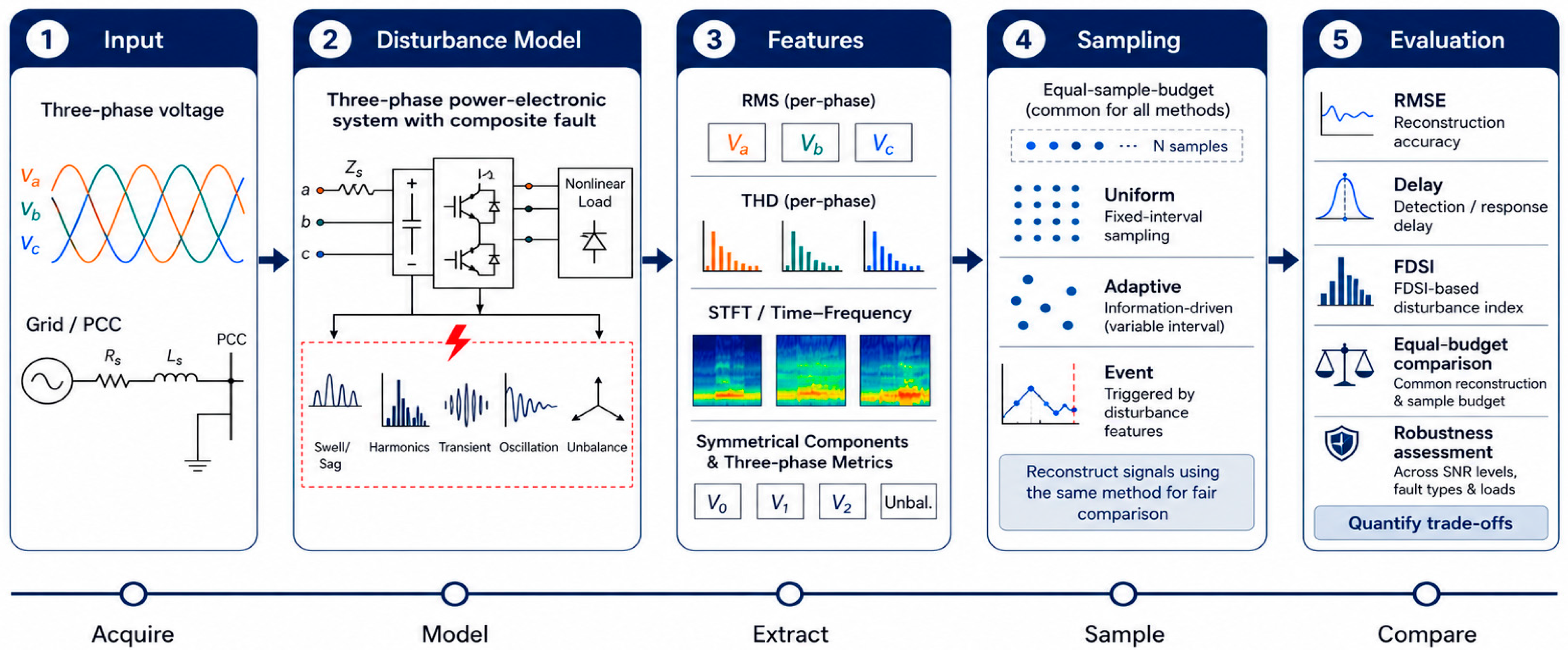
This study presents a controlled MATLAB benchmark to compare uniform, adaptive, and event-triggered sampling under the same three-phase compound disturbance. The methodology comprises five stages: signal generation, disturbance modeling, electrical-feature extraction, sampling and reconstruction, and quantitative performance assessment, as summarized in Figure 1.

A high-resolution three-phase voltage is generated from a grid-connected power-electronic system and modified by a compound disturbance comprising voltage swell, harmonics, a damped transient, low-frequency oscillation, and phase unbalance. RMS, THD, STFT, and symmetrical-component indicators are extracted before applying uniform, adaptive, and event-triggered sampling. The reconstructed signals are then compared using a common reconstruction rule, equal sample budgets, robustness tests, and temporal, spectral, three-phase, and FDSI-based metrics [38,39,40].

2.2. Benchmark Parameterization

Table 2 reports the electrical, disturbance, sampling, and signal-processing parameters used in the MATLAB implementation. The values define the discrete-time benchmark and ensure that all sampling strategies are evaluated using the same three-phase reference signals and compound-disturbance conditions.

The parameters represent a controlled industrial power-quality event rather than a specific field record. The voltage swell, harmonic components, damped transient, low-frequency oscillation, and phase-dependent terms reproduce electrical effects associated with switching operations, nonlinear loads, power electronic converters, and non-ideal three-phase conditions. This parameterization provides known temporal and spectral ground truth for evaluating sampling, reconstruction, and detection performance.

The temporal envelope is discretized as $e\left[n\right]=e\left(n{T}_s\right)$, where $T_s=1/f_s$. A Hann-type transition of duration $t_r$ activates and clears the disturbance between $t_s$ and $t_e$, preventing abrupt numerical discontinuities:

$$e\left(t\right)=\left\{\begin{array}{cc}0,& t<t_s,\\ 0.5\left[1-\cos \left(\pi {\displaystyle \frac{t-t_s}{t_r}}\right)\right],& t_s\le t<t_s+t_r,\\ 1,& t_s+t_r\le t\le t_e-t_r,\\ 0.5\left[1+\cos \left(\pi {\displaystyle \frac{t-\left(t_e-t_r\right)}{t_r}}\right)\right],& t_e-t_r<t\le t_e,\\ 0,& t>t_e,\end{array}\right.$$

(4)

The envelope gradually activates and deactivates the voltage swell, additional harmonics, damped transient, low-frequency oscillation, and phase-unbalance terms. In the present implementation, $t_r=0.05 \mathrm{s}$, while $t_s=5.00 \mathrm{s}$ and $t_e=10.00 \mathrm{s}$. Consequently, the complete disturbance remains confined to the prescribed interval and the mathematical model does not introduce abrupt switching artifacts at its boundaries.

The reference waveforms are generated at a simulation frequency $f_s$, with $T_s=1/f_s$. The discrete three-phase reference signal is expressed as:

$$x\left[n\right]=\left[\begin{array}{c}{x}_a\left[n\right]\\ x_b\left[n\right]\\ x_c\left[n\right]\end{array}\right]=\left[\begin{array}{c}{v}_a\left(n{T}_s\right)\\ v_b\left(n{T}_s\right)\\ v_c\left(n{T}_s\right)\end{array}\right], n=0,1,\dots ,N-1$$

(5)

.

This high-resolution sequence serves as the numerical ground truth for the controlled benchmark. The sampling strategies select different subsets of $x\left[n\right]$, which are subsequently reconstructed on the complete simulation grid. Therefore, the comparison quantifies the performance of each acquisition–reconstruction chain with respect to the same reference waveform and disturbance parameters [41,42,43].

2.3. Qualitative Description of the Composite Disturbance

The benchmark combines five power-quality phenomena within the interval $t_s=5.0 \mathrm{s}$ to $t_e=10.0 \mathrm{s}$: voltage swell, harmonic distortion, a damped transient, low-frequency oscillation, and three-phase unbalance. The phase-dependent swell factors increase the voltage magnitude, while the background and additional harmonic components raise the Phase-A THD from 6.24% to 7.63%. A 120 Hz damped transient with a decay coefficient of $2.0{ \mathrm{s}}^{-1}$ is activated at disturbance inception, and a 5 Hz oscillatory component modifies the voltage envelope. The asymmetric terms $u_a=+0.020$, $u_b=-0.015$, and $u_c=+0.010$ p.u. produce a measurable negative- and zero-sequence response [44,45,46].

This combination represents a controlled industrial disturbance rather than a specific field event. Its purpose is to provide a traceable reference in which temporal, spectral, and asymmetrical effects coexist under known conditions. These characteristics are subsequently evaluated through the three-phase waveform, moving RMS, symmetrical components, THD, and STFT [47].

2.4. Sampling and Reconstruction Criteria

The three sampling strategies are first evaluated using linear interpolation as a common reconstruction method. This controlled comparison isolates the influence of the sampling instants from that of the reconstruction rule. Event-triggered sampling is additionally reconstructed using a zero-order hold to represent its practical digital implementation. Two acquisition conditions are considered. The natural configuration preserves the sample count generated by each strategy, whereas the equal-sample-budget experiment adjusts the adaptive and event-triggered parameters until their final sample counts remain within 1% of the uniform reference. The resulting comparisons therefore distinguish the effects of sampling logic, acquisition density, and reconstruction method.

2.5. Uniform Sampling

Uniform sampling is used as the baseline acquisition strategy. Its sampling instants are defined by:

$$t_n^{\left(u\right)}=n{T}_u, n=0,1,\dots ,N_u-1,$$

(6)

where $T_u=1 \mathrm{ms}$, corresponding to a nominal acquisition rate of $1000$ samples per second, and $N_u$ is the resulting number of acquired samples. The sampled values are $x_k^{\left(u\right)}\left[n\right]=x_k\left(t_n^{\left(u\right)}\right)$. Because the interval remains constant throughout the observation period, uniform sampling provides regular data acquisition and straightforward implementation, although it does not increase its temporal resolution during rapid waveform variations.

For the common-reconstruction comparison, the uniformly sampled signal is reconstructed by linear interpolation between consecutive samples. This reconstruction rule is also applied to the adaptive and event-triggered sample sets when evaluating the isolated effect of the sampling instants. In the practical acquisition-chain comparison, the reconstruction method for each implementation is also reported.

2.6. Adaptive Sampling

Adaptive sampling modifies the acquisition interval according to the local temporal variation in the monitored waveform. To obtain a bounded and dimensionally consistent interval, the local variation is normalized with respect to a reference derivative $G_{\mathrm{ref}}$, and the adaptive sampling interval is defined as:

$$\mathsf{\Delta }{t}_n^{\left(a\right)}=\mathrm{clip}\left[{\displaystyle \frac{\mathsf{\Delta }{t}_{\max }^{\left(a\right)}}{1+\lambda g\left[n\right]}},\mathsf{\Delta }{t}_{\min }^{\left(a\right)}\mathsf{\Delta }{t}_{\max }^{\left(a\right)}\right], g\left[n\right]={\displaystyle \frac{\mid x\left[n\right]-x\left[n-1\right]\mid }{T_s{G}_{\mathrm{ref}}+\epsilon }},$$

(7)

where $g\left[n\right]$ is the normalized local rate of variation, $\lambda$ controls the sensitivity of the adaptive response, and $\epsilon$ prevents numerical division by zero. The operator $\mathrm{clip}\left(\cdot \right)$ constrains the interval between the prescribed minimum and maximum values. In the implemented benchmark, the lower limit prevents excessive oversampling around steep transient variations, whereas the upper limit prevents prolonged intervals without acquisition during slowly varying conditions. The adaptive sampling instants are recursively updated according to:

$$t_{n+1}^{\left(a\right)}=t_n^{\left(a\right)}+\mathsf{\Delta }{t}_n^{\left(a\right)}.$$

(8)

Accordingly, the sampling density increases as the waveform derivative increases and decreases as the signal returns to a slowly varying regime. The adaptive parameters are kept constant throughout each simulation scenario. When an equal-sample-budget comparison is performed, $\lambda$ and the admissible interval limits are adjusted before the simulation so that the resulting sample count remains within the predefined tolerance relative to the uniform-sampling budget. The reconstructed adaptive signal is obtained by linear interpolation, thereby preserving consistency with the common-reconstruction experiment.

2.7. Event-Triggered Sampling

Event-triggered sampling acquires a new value when either the signal variation exceeds a prescribed magnitude threshold or the maximum admissible time without acquisition is reached. The triggering condition is written as:

$$\mathcal{E}\left[m\right]=\left(\mid x\left[m\right]-x\left[n_{\mathrm{last}}\right]\mid \ge \delta \right)\vee \left[\left(m-n_{\mathrm{last}}\right)T_s\ge \mathsf{\Delta }{t}_{\max }\right],$$

(9)

where $n_{\mathrm{last}}$ is the index of the most recently acquired sample, $\delta =0.02 \mathrm{p}.\mathrm{u}.$ is the magnitude-change threshold, and $\mathsf{\Delta }{t}_{\max }=0.01 \mathrm{s}$ is the maximum interval permitted between consecutive acquisitions. When $\mathcal{E}\left[m\right]$ is satisfied, the current point is stored and $n_{\mathrm{last}}$ is updated. The temporal constraint prevents information loss during intervals in which the signal variation remains below the amplitude threshold.

For the methodologically controlled comparison, the event-triggered samples are reconstructed using the same linear interpolation applied to uniform and adaptive sampling. A second result is obtained using zero-order hold, which represents the conventional implementation of event-based digital monitoring and control systems. Under zero-order hold, each acquired value is maintained until the next event is generated. Reporting both reconstruction conditions separates the influence of the sampling logic from the influence of the reconstruction method [39,44,48].

2.8. Performance Evaluation Metrics

The reconstructed signals are evaluated on the complete simulation grid and compared with the high-resolution reference signal. The root mean square error quantifies the average reconstruction deviation and is calculated for each phase and sampling strategy as:

$$RMS{E}_{i,k}=\sqrt{{\displaystyle \frac{1}{N}}{\displaystyle {\displaystyle \sum }_{n=0}^{N-1}}{\left[x_k\left[n\right]-{\widehat{x}}_{i,k}\left[n\right]\right]}^2},$$

(10)

where $i\in \left\{u,a,e\right\}$ identifies the uniform, adaptive, or event-triggered strategy, $k\in \left\{a,b,c\right\}$ identifies the phase, and ${\widehat{x}}_{i,k}\left[n\right]$ is the reconstructed waveform. In addition to the phase-specific values, the three-phase RMSE is obtained by aggregating the squared errors of phases A, B, and C over the same observation interval. The maximum absolute error identifies the largest local reconstruction discrepancy:

$$E_{\max ,i,k}=\underset{0\le n<N}{max}{x}_k\left[n\right]-{\widehat{x}}_{i,k}\left[n\right].$$

(11)

This metric complements the RMSE because a strategy may achieve a low average reconstruction error while still failing to reproduce an isolated transient peak. The reported three-phase maximum error is the largest value across all phases and simulation instants.

The detection time is defined as the first reconstructed-signal instant, after the prescribed disturbance inception, at which the selected detection criterion is satisfied. The corresponding detection delay is

$$D_{t,i,k}=\max \left[0,t_{det,i,k}-t_s\right].$$

(12)

The non-negative constraint avoids interpreting pre-event threshold crossings as negative delays. A common threshold of 1.10 p.u. is applied to all reconstructed signals as a benchmark detection criterion rather than as a universal protection setting [49,50,51].

Spectral preservation is evaluated through the normalized Euclidean difference between the magnitude spectra of the reference and reconstructed signals. Lower spectral-deviation values indicate better retention of the harmonic content.

The reconstruction percentage represents the proportion of the reference waveform retained after reconstruction, bounded between 0% and 100%. The same definition is applied to all strategies and phases. The critical-time error is the absolute difference between the reference instant of maximum distortion and the corresponding instant identified in the reconstructed signal. It therefore measures the temporal accuracy with which each strategy preserves the most severe waveform alteration.

2.9. Metric Normalization

Because the performance indicators have different units and ranges, they are normalized before calculating the composite index. For cost-type metrics, where lower values indicate better performance, the score is

$$S_{i,j}^{\left(-\right)}=1-{\displaystyle \frac{M_{i,j}-M_j^{\min }}{M_j^{\max }-M_j^{\min }+\epsilon }},$$

(13)

where $M_{i,j}$ is the value of metric $j$ for strategy $i$, and $M_j^{\min }$ and $M_j^{\max }$ are the minimum and maximum values within the same experiment. This expression is applied to RMSE, maximum error, detection delay, spectral deviation, and critical-time error. For benefit-type metrics, where higher values are preferable, the score is

$$S_{i,j}^{\left(+\right)}={\displaystyle \frac{M_{i,j}-M_j^{\min }}{M_j^{\max }-M_j^{\min }+\epsilon }}.$$

(14)

This expression is used for the reconstruction percentage. The normalization limits are calculated separately for each experiment and remain fixed during the FDSI weight-sensitivity analysis.

2.10. Fault Detection Sensitivity Index

The normalized metrics are integrated through the Fault Detection Sensitivity Index, introduced in this study as a benchmark-specific multi-criteria indicator:

$${\mathrm{FDSI}}_i=w_{\mathrm{RMSE}}{S}_{i,\mathrm{RMSE}}+w_{E_{\max }}{S}_{i,E_{\max }}+w_{D_t}{S}_{i,D_t}+w_R{S}_{i,R}+w_{\mathrm{SD}}{S}_{i,\mathrm{SD}}+w_{E_c}{S}_{i,E_c}, {\displaystyle \sum }_j{w}_j=1.$$

(15)

The assigned weights are 0.22 for RMSE, 0.14 for maximum error, 0.22 for detection delay, 0.16 for reconstruction percentage, 0.14 for spectral deviation, and 0.12 for critical-time error. At the performance-dimension level, reconstruction fidelity, detection and temporal localization, and signal-information preservation receive total weights of 0.36, 0.34, and 0.30, respectively.

The base weights were assigned according to three monitoring functions represented with comparable overall importance. Reconstruction fidelity combines RMSE and maximum error and receives a total weight of 0.36; detection and temporal localization combine detection delay and critical-time error and receive 0.34; and signal-information preservation combines reconstruction percentage and spectral deviation and receives 0.30. Within each function, the larger weight is assigned to the metric that characterizes its global response, namely RMSE, detection delay, and reconstruction percentage, while the complementary metric captures local or domain-specific deviations. This structure prevents any single performance dimension from dominating the index. The subsequent ±20% perturbation analysis tests whether the reported ordering depends on these nominal coefficients.

The FDSI supports the joint interpretation of the individual metrics and does not replace established power-quality indices. Its robustness is evaluated through weight perturbation and renormalization, while the constituent metrics, sample count, and reconstruction method are reported alongside the composite score.

Table 3. Configuration of the robustness assessment scenarios.

Scenario	Severity Factor	Disturbance Duration [s]	SNR [dB]	Number of Runs	Evaluated Condition
1	1.0	5.0	Noiseless	1	Nominal benchmark
2	0.8	5.0	Noiseless	1	Reduced disturbance severity
3	1.2	5.0	Noiseless	1	Increased disturbance severity
4	1.0	2.5	Noiseless	1	Short-duration disturbance
5	1.0	7.5	Noiseless	1	Extended-duration disturbance
6	1.0	5.0	40	30	Moderate measurement noise
7	1.0	5.0	30	30	Higher measurement noise

summarizes seven representative scenarios used to assess the influence of disturbance severity, duration, and measurement noise. Deterministic cases are evaluated once, while the 40 dB and 30 dB noise conditions use 30 independent Monte Carlo realizations. This compact set captures the principal sources of variability without requiring a full factorial simulation campaign.

2.11. Specific Configuration of the Simulation Scenario

The benchmark was implemented using the parameters in Table 2. Three-phase voltages were generated at 8 kHz, with the compound disturbance applied from $t_s=5.00 \mathrm{s}$ to $t_e=10.00 \mathrm{s}$. The resulting high-resolution signals served as the common numerical reference for temporal, spectral, asymmetry, sampling, and reconstruction analyses.

The evaluation combined phase-specific and aggregated three-phase indicators. RMS, THD, and STFT were used to characterize power-quality degradation, while positive-, negative-, and zero-sequence components and the voltage unbalance factor quantified the asymmetric response [52,53,54].

Two sampling conditions were analyzed. The natural configuration preserved the sample counts produced by each strategy, whereas the equal-sample-budget experiment adjusted the adaptive and event-triggered parameters to keep them within 1% of the uniform reference. Linear interpolation was used for all three strategies in the controlled comparison, and event-triggered sampling was additionally evaluated with zero-order hold.

Performance was evaluated using Equations (10)–(15). Robustness was assessed for different disturbance severities and durations, as well as under 40 dB and 30 dB noise using 30 Monte Carlo realizations per noise level. FDSI sensitivity was examined through 1000 independent weight perturbations of ±20%, from which the score range and ranking stability were obtained. Figure 1 summarizes the complete workflow.

2.12. Pseudocode for Reproducibility

Algorithm 1 summarizes the MATLAB implementation used to reproduce the benchmark. The procedure generates the high-resolution three-phase reference signals, applies the three sampling strategies, reconstructs the sampled waveforms, and computes the phase-specific and aggregated performance indicators. The same disturbance model and reference grid are used throughout the analysis to ensure that the observed differences arise from the sampling, reconstruction, and acquisition conditions.

Algorithm 1. Controlled benchmark for sampling-based monitoring.

Input: - Simulation parameters: $f_s$, $f_0$, $T$, $t_s$, $t_e$, $t_r$ - Disturbance parameters: swell, harmonics, transient, oscillation, unbalance - Sampling parameters: $T_u$, $\Delta t_{min}^{\left(a\right)}$, $\Delta t_{max}^{\left(a\right)}$, $G_{low}$, $G_{high}$, $\delta$, $\Delta t_{guard}$, $\Delta t_{hold,max}$ - Robustness parameters: severity, duration, SNR, number of Monte Carlo runs - FDSI parameters: base weights and perturbation range Output: - Reconstructed three-phase signals, phase-specific and aggregated metrics, equal-budget verification, robustness statistics, and FDSI sensitivity results $\mathbf{Generate} \mathbf{the} \mathbf{time} \mathbf{vector} \mathbf{and} \mathbf{the} \mathbf{Hann}\mathbf{-}\mathbf{type} \mathbf{disturbance} \mathbf{envelope} e\left(t\right)$. $\mathbf{Construct} \mathbf{the} \mathbf{nominal} \mathbf{and} \mathbf{disturbed} \mathbf{voltages} v_a\left(t\right)$$, v_b\left(t\right)$$, \mathbf{and} v_c\left(t\right)$. Compute RMS, THD, STFT, symmetrical components, and VUF. Apply uniform, adaptive, and event-triggered sampling to the same reference signals. Reconstruct all sampled signals using linear interpolation. Reconstruct the event-triggered signal additionally using zero-order hold. Compute, for each phase and strategy, RMSE, maximum error, detection delay, reconstruction percentage, spectral deviation, and critical-time error. Aggregate the phase-specific results into three-phase indicators. Evaluate the natural acquisition configuration and record the resulting sample count. Adjust the adaptive and event-triggered parameters until their sample counts remain within 1% of the uniform reference. Repeat the analysis for the defined severity, duration, and noise scenarios; use 30 Monte Carlo realizations for the 40 dB and 30 dB cases. Normalize the metrics using Equations (13) and (14) and calculate the FDSI using Equation (15). $\mathbf{Perturb} \mathbf{the} \mathbf{FDSI} \mathbf{weights} \mathbf{1000} \mathbf{times} \mathbf{within} \pm \mathbf{20}\mathbf{\%}$, renormalise them, and calculate the minimum, maximum, mean, standard deviation, first-rank probability, and complete-ranking stability. Report the results for the natural, common-reconstruction, equal-budget, robustness, and FDSI-sensitivity experiments.

Algorithm 1 provides a direct link between the mathematical formulation and the reported results. Reconstruction and monitoring performance is quantified through the metrics defined in Equations (10)–(15), while the equal-budget verification controls the effect of acquisition density. The robustness scenarios assess the influence of disturbance severity, event duration, and measurement noise, and the weight-sensitivity analysis determines whether the FDSI ranking remains stable under moderate changes in metric importance.

3. Results

The results are organized to evaluate the benchmark from electrical characterization to sampling performance. First, the temporal, spectral, and asymmetric features of the three-phase disturbance are quantified. The sampling strategies are then compared under common reconstruction, natural acquisition, and equal-sample-budget conditions. Finally, robustness to disturbance variation and measurement noise is assessed together with the sensitivity of the proposed FDSI.

All results are obtained from the same high-resolution three-phase reference signals, with the compound disturbance applied from $t_s=5.00 \mathrm{s}$ to $t_e=10.00 \mathrm{s}$. Phase-specific and aggregated three-phase indicators are reported to account for the unbalance included in the benchmark. Graphical and quantitative results are presented throughout this section according to the corresponding analysis.

To improve the traceability of the results,

Table 4. Summary of the principal quantitative results obtained from the controlled benchmark.

Analysis Dimension	Main Indicator	Value	Interpretation
Disturbance definition	Disturbance interval	5.00–10.00 s	Finite compound-disturbance window
Voltage excursion	Phase-A maximum	1.514 p.u. at 5.3874 s	Maximum instantaneous voltage during the event
Harmonic distortion	Phase-A THD	6.24% to 7.63%	Increase of 1.39 percentage points
Relative harmonic variation	Relative THD increase	22.3%	Measurable spectral degradation
Three-phase asymmetry	VUF	0% to 0.929%	Mild but measurable voltage unbalance
Natural acquisition effort	Sample count	U: 9001; A: 23,524; E: 16,328	Data volume produced by each sampling rule
Best natural reconstruction	Three-phase RMSE	Event-triggered: 0.03020 p.u.	Lowest aggregate reconstruction error
Highest natural reconstruction	Reconstruction percentage	Event-triggered: 96.149%	Highest retained waveform fidelity
Fastest natural detection	Detection delay	Event-triggered: 0.007750 s	Shortest disturbance-localization delay
Natural composite performance	FDSI	U: 0.60574; A: 0.21741; E: 0.99989	Composite result under common linear reconstruction
Equal-budget outcome	Sample count	U: 9001; A: 9000; E: 8981	Maximum deviation of 0.2222% from the target
Equal-budget trade-off	FDSI	U: 0.77818; A: 0.19748; E: 0.77189	Uniform and event-triggered provide comparable composite performance

Abbreviations: U, uniform; A, adaptive; E, event-triggered.

summarizes the principal quantitative indicators obtained from the temporal, spectral, and monitoring analyses. It provides a concise overview of the relationships among the model variables, disturbance behavior, and sampling-performance metrics.

3.1. Temporal Characterization of the Three-Phase Disturbance

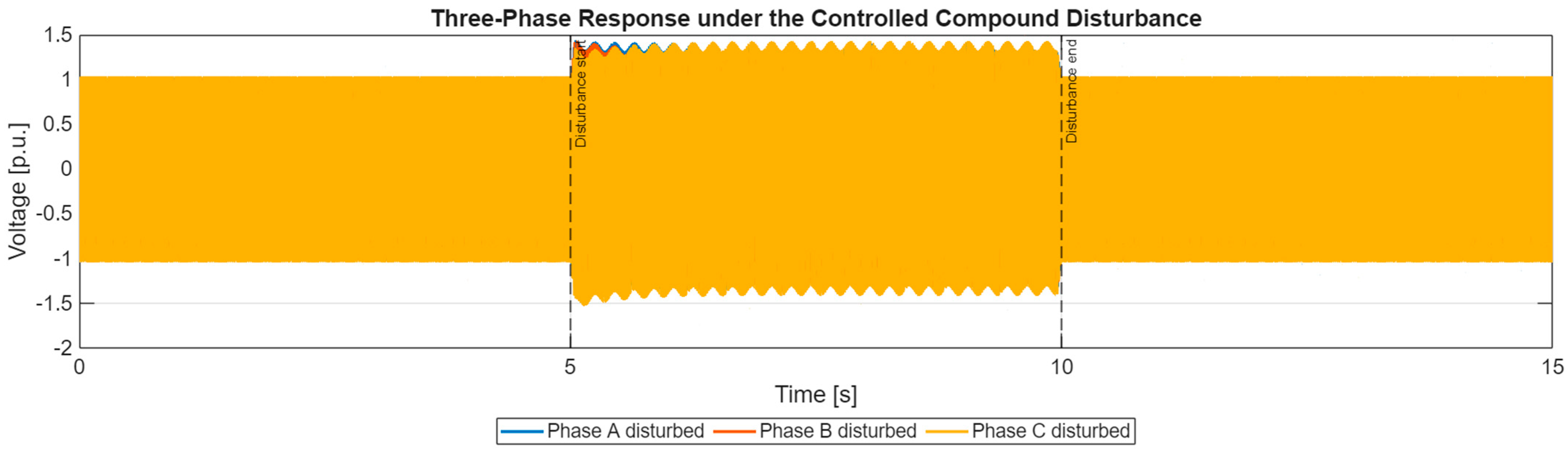
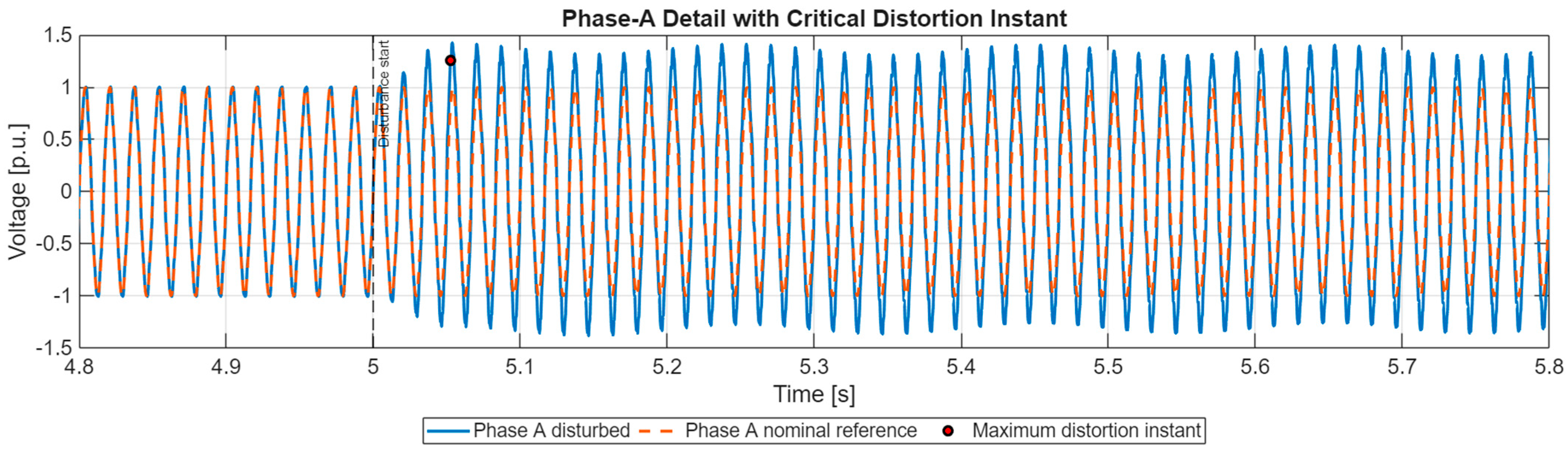
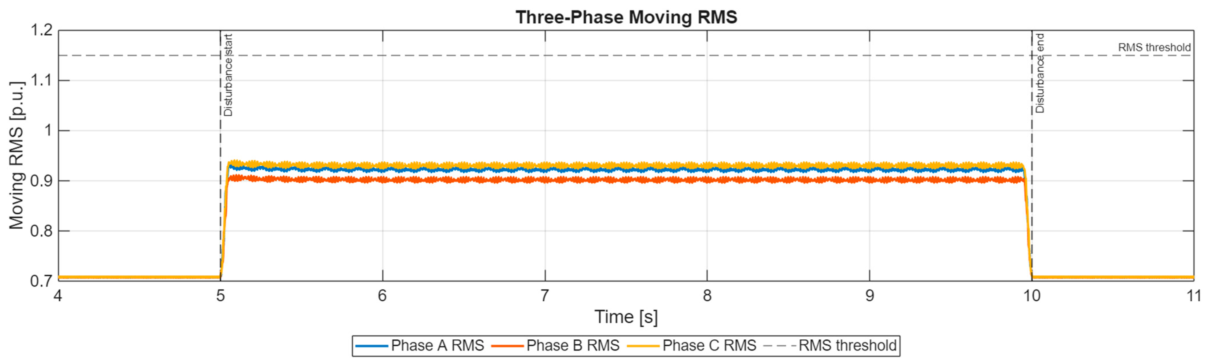
Figure 2, Figure 3 and Figure 4 characterize the temporal input signals at global, local, and cycle-averaged levels. Figure 2 shows that the three-phase waveform remains within its nominal amplitude range before $t=5 \mathrm{s}$ and returns to this condition after $t=10 \mathrm{s}$.

Within the prescribed disturbance interval, the voltage envelope increases from approximately 1 p.u. to peak values close to 1.4 – 1.5 p.u. The transition remains confined to the analytical disturbance window, confirming that the temporal envelope activates and clears the compound event without extending its effect into the nominal intervals.

The complete 15 s representation intentionally shows the sustained modification of the voltage envelope; however, the individual cycles are resolved more clearly in Figure 3. The Phase-A detail around the disturbance inception shows that the nominal and disturbed signals coincide before $t=5$ s, after which the smooth ramp introduces the voltage swell and the superimposed oscillatory components. The maximum distortion instant occurs shortly after inception, during the interval in which the damped transient, harmonic injection, and amplitude transition coexist. This local condition defines a demanding reconstruction interval because the signal combines a rapid envelope variation with non-sinusoidal content.

The moving-RMS values in Figure 4 provide a cycle-based representation of the three-phase amplitude change. Before the event, the RMS remains close to $1/\sqrt{2}$, approximately 0.707 p.u., as expected for a unit-peak sinusoidal voltage. During the disturbance, the phase RMS values increase to approximately 0.90–0.93 p.u., with Phase B exhibiting the lowest value and Phase C the highest. The separation between the phase RMS trajectories confirms that the disturbance modifies both the common voltage magnitude and the relative three-phase balance. The RMS values remain below the 1.15 p.u. monitoring threshold; therefore, the benchmark cannot be fully characterized through a single amplitude criterion and requires the complementary spectral and asymmetry indicators presented below.

Taken together, Figure 2, Figure 3 and Figure 4 establish the temporal ground truth used by the sampling experiments. The global waveform identifies the finite disturbance interval, the local view resolves the transition and the critical distortion point, and the RMS trajectories quantify the sustained phase-dependent amplitude change. These signal characteristics reproduce conditions relevant to converter-fed industrial networks, variable-speed drives, UPS systems, and microgrids, where a disturbance may combine a persistent voltage variation with short-duration components that require different acquisition resolutions.

3.2. Three-Phase Asymmetry and Time-Frequency Content

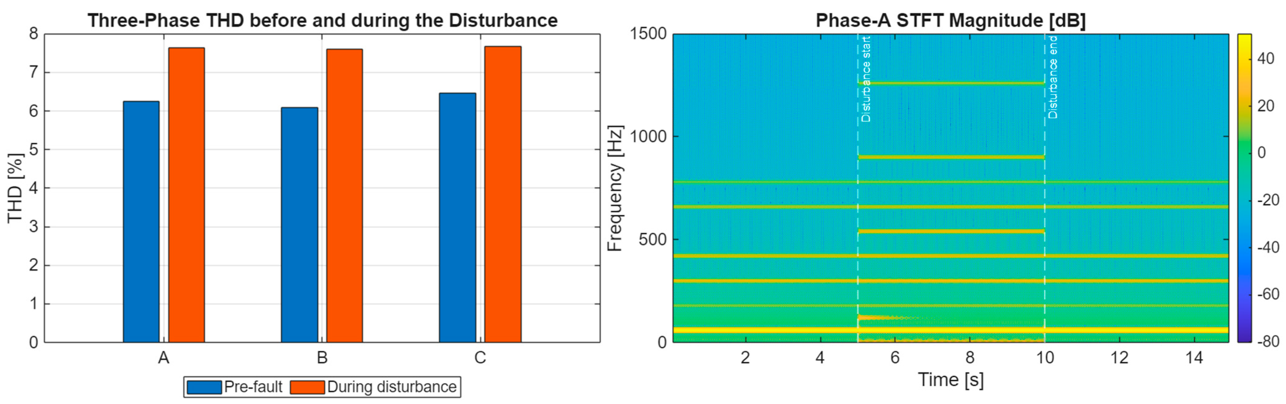
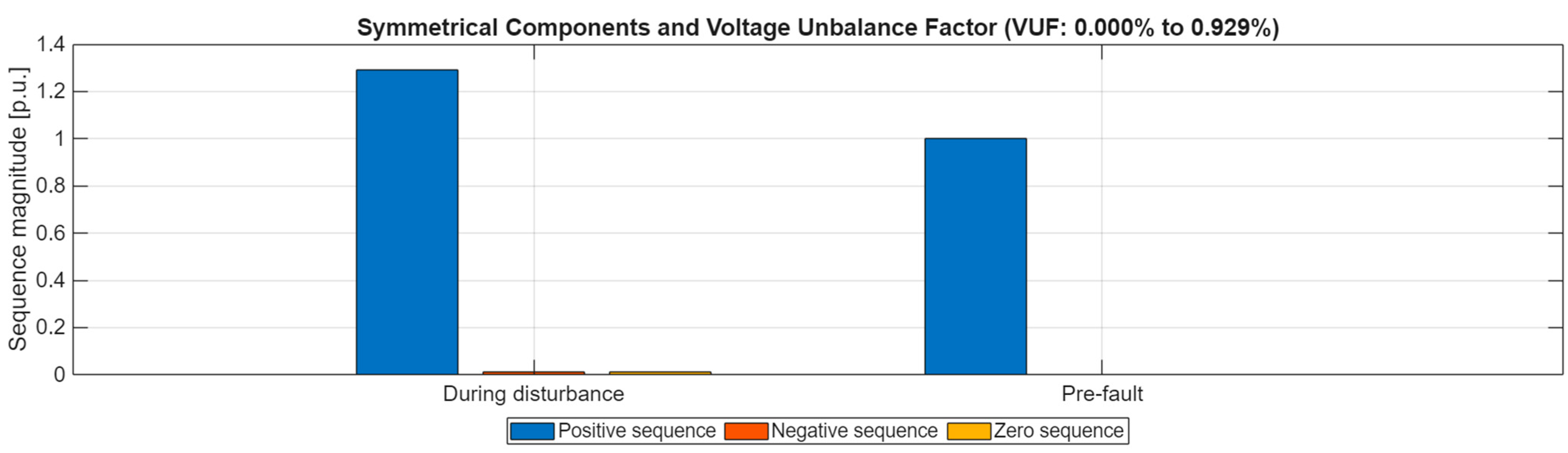
Figure 5 and Figure 6 extend the assessment from time-domain amplitude to sequence components, harmonic distortion, and time-frequency localization. The symmetrical-component results in Figure 5 show that the pre-disturbance voltage is dominated by the positive sequence, with negligible negative- and zero-sequence components. During the compound event, the positive-sequence magnitude increases to approximately 1.29 p.u., while measurable negative- and zero-sequence components appear. The resulting voltage unbalance factor increases from approximately 0% to 0.929%.

The sequence-component result verifies that the phase-dependent terms of the analytical model produce an electrically interpretable asymmetric condition rather than three independently distorted waveforms. A VUF of 0.929% represents a mild but clearly measurable imbalance, allowing the benchmark to assess whether the reconstruction procedures retain information associated with the negative sequence. This characteristic is relevant to monitoring systems for three-phase converters, induction motors, distributed generation interfaces, and industrial loads, where low levels of voltage asymmetry may affect current balance, thermal stress, and control performance.

Figure 6 combines the three-phase THD results with the Phase-A STFT. The THD increases in all phases during the disturbance. For Phase A, it rises from approximately 6.24% to 7.63%, equivalent to an increase of 1.39 percentage points or about 22.3% relative to the pre-disturbance value. Phases B and C exhibit a comparable increase, demonstrating that the additional harmonic content affects the complete three-phase system rather than a single selected signal.

The STFT localizes this spectral modification between 5 and 10 s. In addition to the persistent 60 Hz component, the map exhibits reinforced frequency bands during the disturbance, including components associated with the added harmonics and the 120 Hz transient. The simultaneous changes in THD, time-frequency energy, and sequence components indicate that the generated event contains temporal, spectral, and asymmetric information. Consequently, the subsequent sampling comparison evaluates the ability to preserve a compound diagnostic signature, not merely the amplitude of a voltage swell.

The principal electrical indicators derived from the input signals are summarized in

Table 5. Quantitative characterization of the three-phase compound disturbance.

Indicator	Pre-Disturbance	During Disturbance	Variation
Positive-sequence magnitude [p.u.]	1.0000	1.2933	+29.33%
Negative-sequence magnitude [p.u.]	$5.14\times {10}^{-15}$	0.012018	+0.012018 p.u.
Zero-sequence magnitude [p.u.]	$7.57\times {10}^{-15}$	0.012041	+0.012041 p.u.
Voltage unbalance factor [%]	$\approx 0$	0.92925	+0.92925 percentage points
Phase-A THD [%]	6.24	7.63	+1.39 percentage points
Phase-A relative THD increase [%]	—	—	22.3
Moving RMS [p.u.]	$\approx 0.707$	0.90–0.93	approximately +27–32%

. The results confirm that the disturbance simultaneously modifies the voltage magnitude, harmonic content, and phase symmetry. The positive-sequence component increases from 1.0000 to 1.2933 p.u., while the negative- and zero-sequence components reach approximately 0.012 p.u., producing a VUF of 0.929%. These values provide the three-phase electrical basis for the subsequent sampling analysis.

The sequence components confirm that the pre-disturbance system is practically balanced, whereas the compound event introduces measurable negative- and zero-sequence voltages and increases the VUF to 0.929%. In parallel, Phase-A THD rises by 1.39 percentage points, corresponding to a relative increase of 22.3%, while the moving RMS increases to approximately 0.90–0.93 p.u. These results confirm the simultaneous amplitude, spectral, and asymmetric degradation represented by the benchmark.

3.3. Common-Reconstruction Comparison of the Sampling Strategies

Figure 7, Figure 8 and Figure 9 compare uniform, adaptive, and event-triggered sampling using the same linear-interpolation method. Applying a common reconstruction rule removes a methodological source of bias and allows differences in the reconstructed signals to be associated primarily with the distribution of the sampling instants.

Uniform sampling in Figure 7 produces a regular representation of the disturbed voltage because its acquisition instants remain equally spaced before and after the event. The reconstructed curve consistently follows the reference signal over the displayed interval, while the uniform temporal distribution yields predictable data throughput and a homogeneous reconstruction pattern. Its fixed acquisition rate, however, cannot reallocate samples specifically towards the disturbance transition or local high-slope regions.

Adaptive sampling in Figure 8 adjusts its local acquisition density based on the temporal variation in the waveform. The acquired points become more concentrated in regions with larger derivatives, particularly after the disturbance inception and around local extrema. The reconstructed signal retains the main voltage envelope and oscillatory structure, although the phase-specific results presented later show that the benefit depends on the signal phase and the acquisition budget assigned to the method.

Event-triggered sampling in Figure 9 stores new data when the signal change exceeds the prescribed threshold or when the maximum admissible interval is reached. Under linear interpolation, the reconstructed waveform closely follows the reference signal throughout the displayed interval. This result demonstrates that the reduced reconstruction performance previously associated with event-triggered acquisition cannot be attributed exclusively to its sampling rule; part of that behavior was produced by the use of a zero-order hold in the practical reconstruction chain.

The joint interpretation of Figure 7, Figure 8 and Figure 9, therefore, separates two effects that were combined in the original analysis. The common-reconstruction experiment evaluates how the sampling instants represent the waveform, whereas the subsequent zero-order-hold experiment evaluates the practical digital implementation of the event-triggered strategy. This distinction strengthens the comparison because linear interpolation is not implicitly favored across the two strategies, whereas a different reconstruction mechanism is imposed on the third.

3.4. Natural Acquisition Effort, Equal-Sample-Budget Comparison, and Phase-Specific Performance

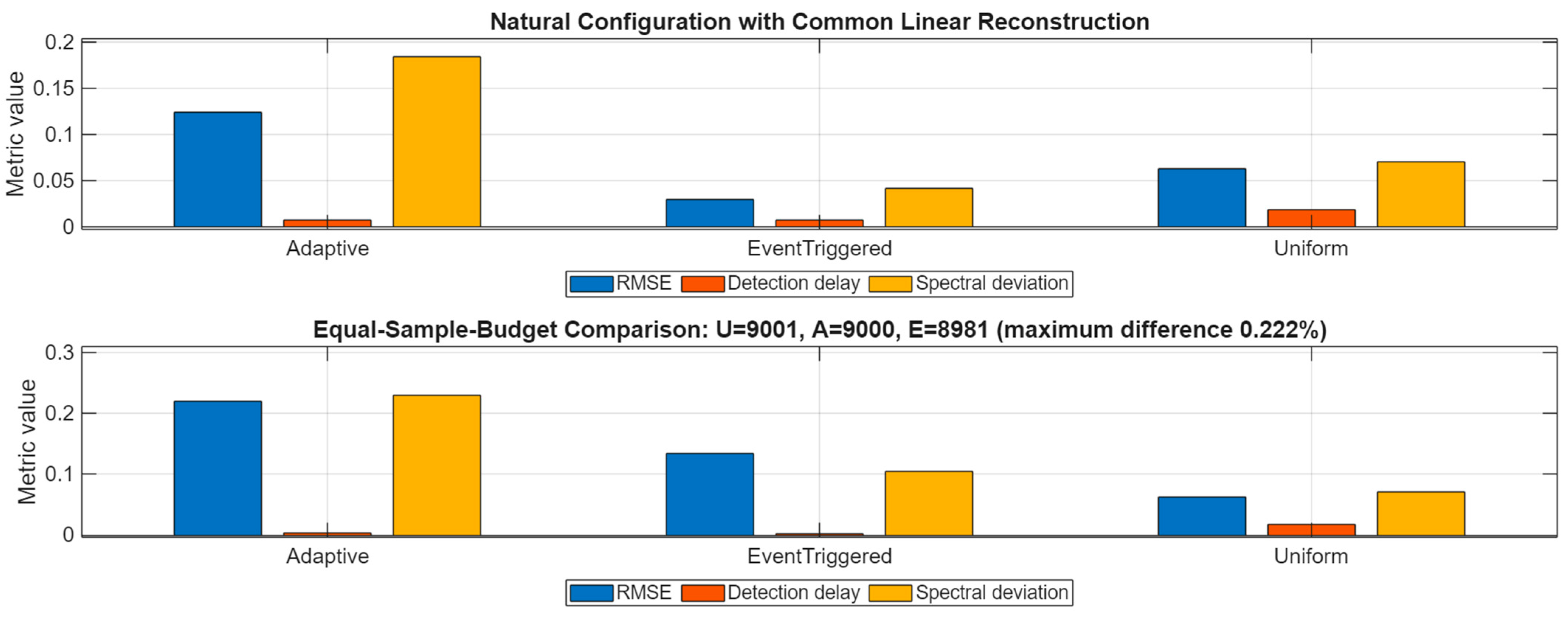
Figure 10, Figure 11, Figure 12, Figure 13, Figure 14 and Figure 15 provide complementary analyses that cannot be inferred from a single performance table. They separately examine phase dependence, robustness to noise and severity, FDSI weight sensitivity, reconstruction-rule effects, and the relationship between acquisition effort and monitoring performance. The comparison is therefore representative of how the strategies would operate when their internal parameters are not forced to achieve identical data volumes. The equal-budget experiment controls the influence of acquisition density. Uniform, adaptive, and event-triggered sampling used 9001, 9000, and 8981 samples, respectively, with a maximum deviation of 0.222%, well below the 1% tolerance. Under this condition, uniform sampling achieved the lowest RMSE and highest reconstruction percentage, whereas event-triggered sampling retained the shortest detection delay and lowest critical-time error.

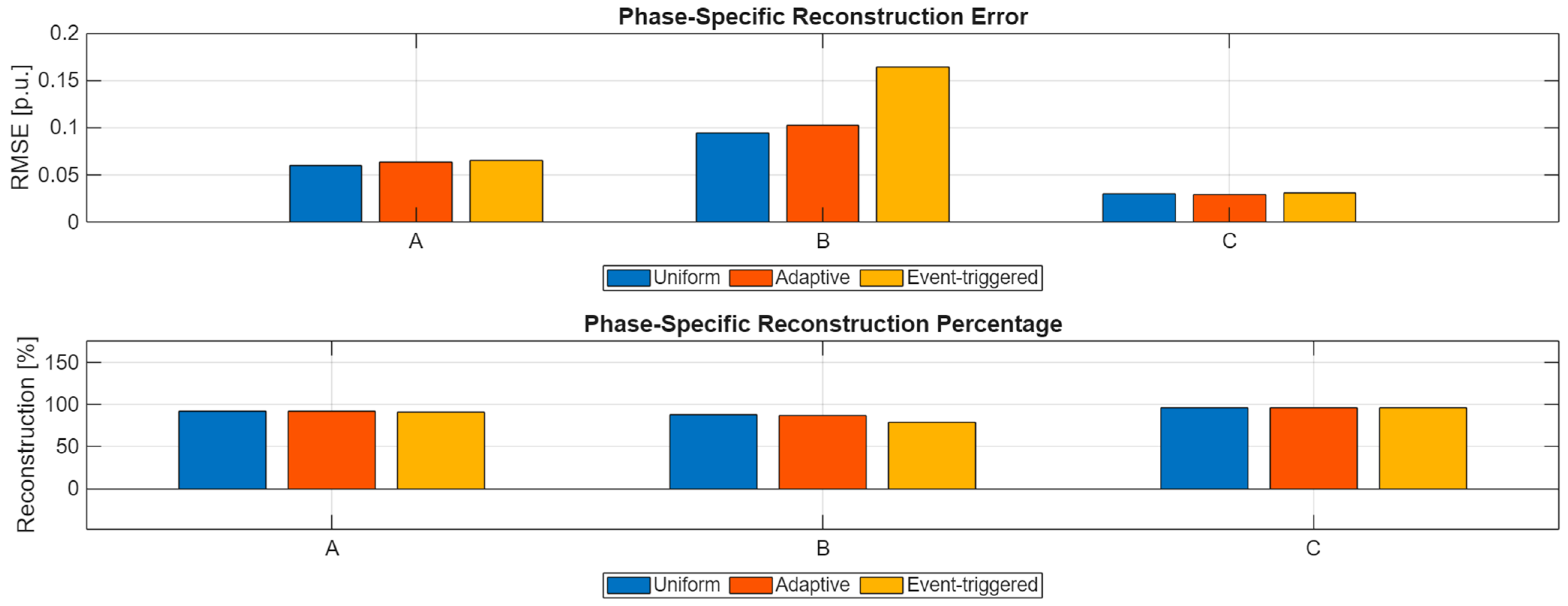
Figure 10 shows that Phase B is the most demanding signal for the three strategies. Event-triggered sampling reaches a Phase-B RMSE of approximately 0.16 p.u. and a reconstruction percentage close to 79%, while Phase C remains near 96%. This phase-dependent response confirms the need for aggregated three-phase indicators rather than a Phase-A-only assessment.

Table 6. Three-phase performance under the natural acquisition configuration.

Method	Ns	RMSE [p.u.]	emax [p.u.]	Dt [s]	(R) [%]	Dsp	Ect [s]	FDSI
Uniform	9001	0.06330	0.26790	0.018375	91.929	0.071062	0.089625	0.60574
Adaptive	23,524	0.12444	1.10960	0.007875	84.647	0.184520	4.808500	0.21741
Event-triggered	16,328	0.03020	0.20706	0.007750	96.149	0.041599	0.094000	0.99989

Note: $N_s$, sample count; $e_{\max }$, maximum error; $D_t$, detection delay; $R$, reconstruction percentage; $D_{\mathrm{sp}}$, spectral deviation; $E_{\mathrm{ct}}$, critical-time error.

reports the natural-configuration results obtained with common linear reconstruction. Event-triggered sampling yields the lowest RMSE, maximum error, detection delay, and spectral deviation, and the highest reconstruction percentage. Uniform sampling maintains an intermediate, regular profile, whereas adaptive sampling allocates the largest acquisition budget and exhibits greater sensitivity to the alignment between its derivative-based sampling instants and the compound waveform.

Event-triggered sampling reduces the three-phase RMSE by 52.3% relative to uniform sampling and by 75.7% relative to adaptive sampling. It also achieves the highest reconstruction percentage, 96.149%, despite using fewer samples than the adaptive strategy. These results show that sample placement is more influential than acquisition density alone when all strategies use the same reconstruction method.

To control the effect of sample count, the adaptive and event-triggered parameters were adjusted using the uniform configuration as the reference, as reported in

Table 7. Equal-sample-budget verification and three-phase performance.

Method	Budget Target/Final ΔN [%]	RMSE [p.u.]	emax [p.u.]	Dt [s]	R [%]	Dsp	Ect [s]	FDSI
Uniform	9001/9001 (0.0000)	0.06330	0.26790	0.018375	91.929	0.071062	0.089625	0.77818
Adaptive	9001/9000 (0.0111)	0.21945	1.09530	0.004125	73.133	0.230490	4.833700	0.19748
Event-triggered	9001/8981 (0.2222)	0.13398	0.45961	0.002500	84.051	0.104120	0.016500	0.77189

Note: All final sample counts satisfy the predefined 1% tolerance. $\mathsf{\Delta }N$ denotes the relative difference from the target budget. The remaining abbreviations follow Table 6.

. The final counts were 9001, 9000, and 8981 samples, with a maximum deviation of 0.2222%, thereby satisfying the predefined 1% tolerance.

The equal-budget experiment modifies the balance observed under the natural configuration. Uniform sampling achieves the lowest RMSE, 0.06330 p.u., and the highest reconstruction percentage, 91.929%, whereas event-triggered sampling retains the shortest detection delay, 0.0025 s, and the lowest critical-time error, 0.0165 s. Their FDSI values are comparable, at 0.77818 and 0.77189, respectively, indicating that the preferred strategy depends on whether the monitoring objective prioritizes global waveform reconstruction or rapid temporal localization.

Adaptive sampling is the most sensitive to the restricted acquisition budget. Its reconstruction percentage decreases to 73.133%, while the RMSE increases to 0.21945 p.u. The equal-budget configuration was obtained using an upper slope threshold of 235.7753 and an event-trigger threshold of 0.307116 p.u., which define the reproducible operating conditions of this comparison.

Figure 11 resolves the aggregated sampling results by phase. The phase-dependent differences in RMSE and reconstruction percentage confirm that the imposed unbalance affects the three signals differently and that a Phase-A-only evaluation would not represent the complete system response.

The phase-resolved results confirm that the aggregated indicators reflect distinct three-phase behavior. Uniform sampling provides the most consistent reconstruction across phases, whereas adaptive and event-triggered sampling are more sensitive to local waveform variations. This response is consistent with the sequence-component results in Figure 5.

3.5. Robustness to Measurement Noise and Disturbance Variation

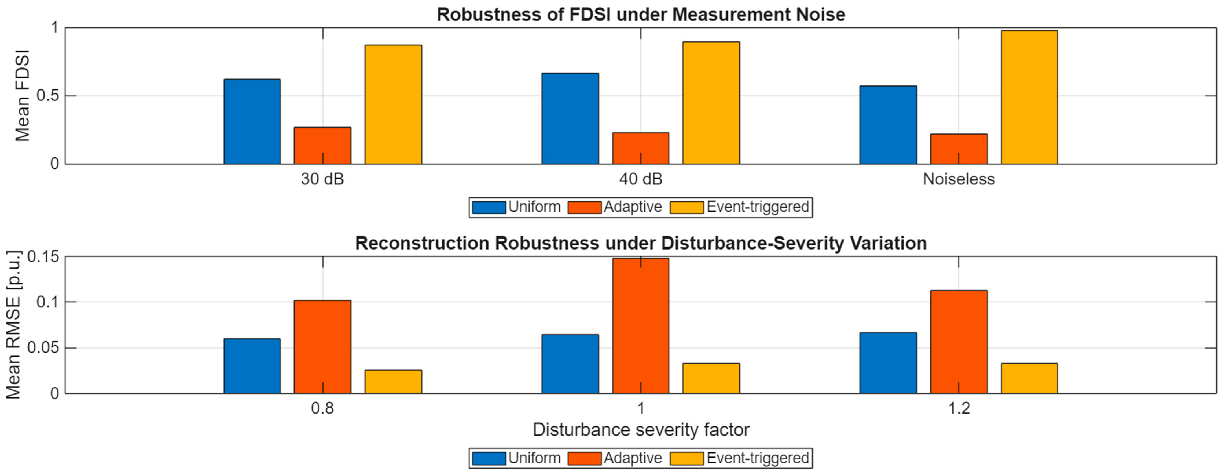
Figure 12 evaluates robustness under measurement noise and disturbance-severity variation. The Monte Carlo results at 40 dB, and 30 dB distinguish the influence of random noise from the deterministic response, while the severity analysis shows how each sampling rule reacts to changes in disturbance magnitude.

The 30 dB and 40 dB cases were evaluated using 30 independent Monte Carlo realizations. The preserved performance order across both noise levels indicates that the observed behavior is not dependent on a particular noise sequence. The reduction in FDSI under noisier conditions reflects the combined degradation of reconstruction accuracy, spectral preservation, and event localization.

The lower panel of Figure 12 shows the mean three-phase RMSE for severity factors of 0.8, 1.0, and 1.2. Uniform sampling varies only from approximately 0.06 to 0.067 p.u., while event-triggered sampling remains below 0.035 p.u. Adaptive sampling exhibits the largest variation, reaching approximately 0.15 p.u. at the nominal severity. This non-monotonic response is consistent with its slope-dependent acquisition rule, since changes in disturbance severity modify the instants at which the sampling interval contracts or expands.

Overall, event-triggered sampling provides the most stable composite performance under the analyzed conditions, uniform sampling maintains the most regular response, and adaptive sampling remains more sensitive to parameter tuning and acquisition density. These differentiated behaviors support their use in complementary monitoring functions rather than as interchangeable strategies.

3.6. FDSI Weight Sensitivity and Ranking Stability

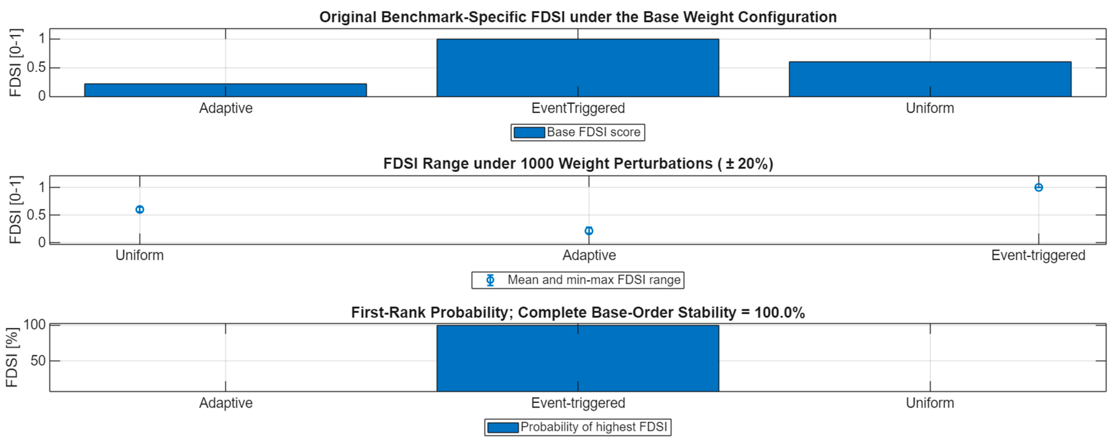
Figure 13 examines whether the FDSI ranking depends on the selected weighting structure. The score ranges obtained from 1000 independent perturbations of ±20% quantify index variability and verify the stability of the resulting strategy order.

The second panel shows the mean and minimum–maximum FDSI ranges obtained from 1000 independent weight perturbations of $\pm 20\%$. The ranges remain clearly separated, indicating limited sensitivity to moderate changes in metric importance. Event-triggered sampling retains the first position in 100% of the tested cases, and the complete base ranking is also preserved in 100% of the perturbations.

The corresponding statistics are reported in

Table 8. FDSI sensitivity under 1000 independent weight perturbations.

Method	Base	Mean	SD	Minimum	Maximum	Pfirst [%]
Uniform	0.60574	0.60657	0.016989	0.56057	0.65032	0
Adaptive	0.21741	0.21645	0.021078	0.16597	0.27514	0
Event-triggered	0.99989	0.99989	(1.253\times ×10−5)	0.99986	0.99991	100

Note: SD, standard deviation; $P_{\mathrm{first}}$, probability of obtaining the first-ranked FDSI.

. These results confirm that the ranking is determined by the separation among the underlying performance metrics rather than by a narrowly selected set of weights.

The event-triggered FDSI shows the lowest variability, with a standard deviation of $1.253\times {10}^{-5}$ and a range of $5\times {10}^{-5}$. Uniform and adaptive sampling exhibit wider ranges of 0.08975 and 0.10917, respectively, while the ranking remains unchanged: Event-triggered $>$ Uniform $>$ Adaptive. This result shows that the ranking is driven by the constituent reconstruction, detection, spectral, and temporal metrics rather than by a specific weight combination. The FDSI should therefore be interpreted as a benchmark-specific composite metric and reported together with its individual indicators.

3.7. Influence of the Reconstruction Rule and Metrics for External Comparison

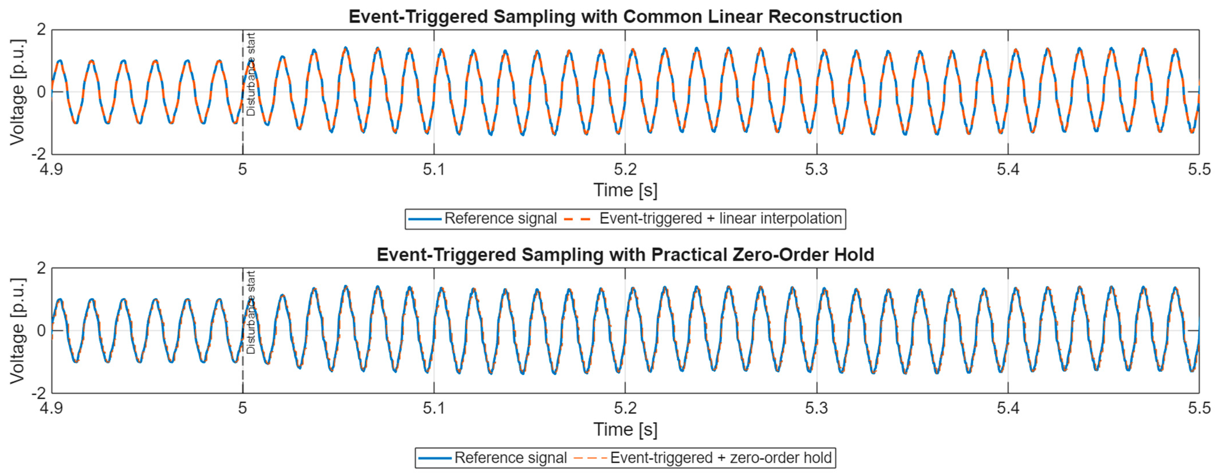
Figure 14 separates the influence of event-triggered acquisition from that of the reconstruction rule. Comparing linear interpolation and zero-order hold using the same event samples shows how reconstruction affects local waveform fidelity without changing the underlying sampling instants.

The similarity between the two panels confirms that the event-triggered sampling instants preserve the main disturbance structure. However, the reconstruction rule affects the local waveform shape: zero-order hold introduces step-like deviations, whereas linear interpolation provides a smoother approximation between consecutive events. Reporting both cases, therefore, separates the effect of event-based acquisition from that of the reconstruction method. Zero-order hold remains suitable for low-complexity alarm systems, while linear interpolation offers higher fidelity for diagnostic analysis using the same sample sequence.

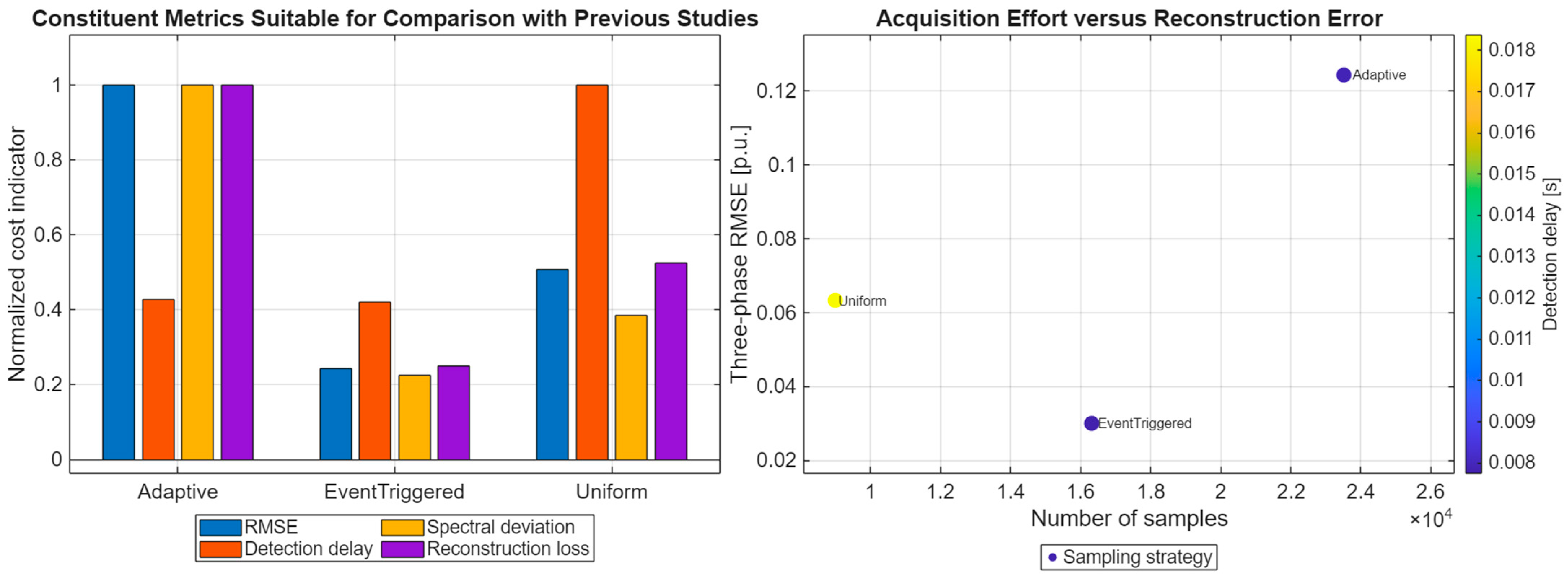
Figure 15 relates acquisition effort to reconstruction and detection performance. Unlike the metric tables, this representation directly shows the trade-off between sample count, three-phase RMSE, spectral preservation, and temporal response, thereby supporting strategy selection according to the monitoring objective.

The right panel relates acquisition effort to three-phase RMSE. Event-triggered sampling achieves the lowest error with fewer samples than adaptive sampling, while uniform sampling uses the smallest acquisition budget and maintains an intermediate RMSE. These results show that sample count alone does not determine reconstruction quality; the temporal distribution of the acquired points and the reconstruction rule are equally decisive.

Figure 15 links acquisition effort with three-phase reconstruction performance. Uniform sampling uses approximately 9000 samples and yields an RMSE of 0.063 p.u. Event-triggered sampling uses about 16,300 samples and reduces the RMSE to 0.030 p.u., whereas adaptive sampling requires approximately 23,500 samples and reaches 0.124 p.u. under the natural configuration.

These results show that acquisition density alone does not determine reconstruction quality. Event-triggered sampling achieves the most efficient balance between sample count, reconstruction error, and detection speed, while uniform sampling provides the lowest data volume with stable intermediate performance.

Adaptive sampling remains more sensitive to parameter tuning and sample placement. The constituent metrics, therefore, provide a suitable basis for comparison with previous monitoring approaches, provided that the disturbance model, reconstruction method, and metric definitions are reported consistently.

3.8. Synthesis of Findings and Strategy Selection According to Operational Objective

The revised experiments show that sampling performance depends on the interaction among acquisition logic, reconstruction method, sample budget, and monitoring objective. Under the natural configuration with common linear reconstruction, event-triggered sampling achieves the lowest three-phase RMSE (0.0302 p.u.), the highest reconstruction percentage (96.149%), and the shortest detection delay (7.75 ms). Uniform sampling yields a stable intermediate response with 9001 samples and an RMSE of 0.0633 p.u., whereas adaptive sampling requires 23,524 samples and exhibits greater sensitivity to parameter tuning and phase-dependent waveform variation.

The equal-sample-budget experiment provides a complementary interpretation. With final counts of 9001, 9000, and 8981 samples, uniform sampling achieves the lowest RMSE and highest reconstruction percentage, while event-triggered sampling preserves the shortest detection delay and the lowest critical-time error. Their FDSI values remain close, at 0.77818 and 0.77189, respectively. This result indicates that uniform sampling is preferable when global waveform fidelity is prioritized under a fixed data budget, whereas event-triggered sampling is more suitable when rapid localization of the disturbance is required.

The robustness analysis supports these differentiated roles. Event-triggered sampling retains the highest composite performance under noiseless, 40 dB, and 30 dB conditions and remains comparatively stable across the severity levels analyzed. Uniform sampling exhibits the most regular behavior across phases and operating conditions. Adaptive sampling responds more strongly to changes in severity, sample budget, and slope thresholds, indicating that its effectiveness depends on careful parameter adjustment to the expected disturbance dynamics.

These results support a layered monitoring architecture rather than the use of a single strategy for all functions. Uniform sampling can provide continuous baseline supervision with predictable data throughput. Event-triggered sampling can operate as a rapid detection and selective-acquisition layer, reducing unnecessary measurements during stationary intervals. Adaptive sampling can be activated for detailed post-event analysis when its parameters are tuned to the disturbance class and a larger acquisition budget is available.

Such an architecture is applicable to converter-fed industrial networks, renewable-energy interfaces, UPS systems, variable-speed drives, microgrids, and digital shadow or digital twin platforms. By separating baseline acquisition, rapid event localization, and high-resolution diagnostic reconstruction, the proposed framework links sampling performance with practical requirements for storage, communication, processing, and decision support.

4. Discussion

The revised benchmark provides a controlled framework for evaluating sampling-based monitoring under a compound three-phase power-quality disturbance. The simultaneous presence of voltage swell, harmonic distortion, a damped transient, low-frequency oscillation, and phase unbalance enables assessment of the temporal, spectral, and asymmetric response under known and reproducible conditions. The increase in Phase-A THD from 6.24% to 7.63%, together with a VUF of 0.929%, confirms that the benchmark contains measurable harmonic and three-phase degradation beyond a simple amplitude variation.

The sampling comparison shows that performance depends on acquisition logic, reconstruction method, and data budget. Under the natural configuration with common linear reconstruction, event-triggered sampling achieved the lowest three-phase RMSE, 0.03020 p.u., the highest reconstruction percentage, 96.149%, and the shortest detection delay, 7.75 ms. Uniform sampling required the fewest samples and maintained intermediate reconstruction performance, whereas adaptive sampling used the largest acquisition budget and showed greater sensitivity to parameter tuning and phase-dependent waveform variation.

The equal-sample-budget experiment provides a different operational interpretation. With 9001, 9000, and 8981 samples, uniform sampling achieved the lowest RMSE and highest reconstruction percentage, while event-triggered sampling retained the shortest detection delay and lowest critical-time error. Their FDSI values were close, at 0.77818 and 0.77189, respectively. Thus, uniform sampling is preferable when global reconstruction under a fixed data budget is prioritized, whereas event-triggered sampling is more suitable for rapid event localization.

The robustness analysis supports these differentiated roles. Event-triggered sampling retained the highest composite response under noiseless, 40 dB, and 30 dB conditions, while uniform sampling exhibited the most regular behavior across phases and disturbance severities. Adaptive sampling remained more dependent on the selected slope thresholds and available sample budget. These results support a layered monitoring architecture in which uniform sampling provides baseline supervision, event-triggered acquisition supports rapid detection, and adaptive sampling is activated for detailed post-event analysis when its parameters can be tuned to the disturbance class.

From a technical perspective, the proposed benchmark and digital-twin-based monitoring address different stages of the validation process. The proposed framework operates with mathematically defined ground-truth signals, controlled disturbance parameters, fixed reconstruction rules, and explicitly constrained acquisition budgets. These characteristics allow the isolated evaluation of sampling placement, reconstruction accuracy, detection delay, spectral preservation, and three-phase asymmetry without the influence of plant-model uncertainty, communication latency, synchronization errors, or sensor dynamics. In contrast, a digital twin continuously interacts with a physical asset through field measurements, model updating, communication infrastructure, and real-time computational processes. Therefore, digital-twin performance depends not only on the monitoring algorithm but also on model fidelity, parameter identification, data quality, communication delays, and synchronization between the physical and virtual systems. The novelty of the proposed approach lies in its reproducible and low-complexity pre-validation environment. This framework enables the intrinsic performance of the sampling strategies to be quantified before their integration into a digital twin, digital shadow, hardware-in-the-loop platform, or field-monitoring architecture. The two approaches are therefore complementary rather than interchangeable: the proposed benchmark supports controlled algorithmic pre-validation, whereas digital-twin platforms provide the subsequent environment for online supervision, model updating, prediction, and decision support.

A complete quantitative comparison with an operational digital twin, including computational burden, communication latency, online model adaptation, synchronization accuracy, and real-time implementation, is beyond the scope of the present simulation-based benchmark and will be addressed in future research using hardware-in-the-loop and field-measurement platforms.

The main limitation is the study’s simulation-based nature. Although the revised analysis includes three-phase indicators, common reconstruction, equal sample budgets, disturbance variation, measurement noise, Monte Carlo assessment, and FDSI sensitivity, experimental validation with field or hardware-in-the-loop data remains necessary. In addition, the benchmark parameters represent a controlled disturbance rather than a specific network event. The FDSI should therefore be interpreted as an original benchmark-specific composite metric and always be considered together with its constituent indicators.

Comparison with Existing Monitoring Approaches

Because the FDSI is introduced in this study, its absolute values cannot be compared directly with previous publications. External comparison should instead use the constituent metrics reported in

Table 9. Constituent metrics available for comparison with previous studies.

Method	Ns	RMSE [p.u.]	emax [p.u.]	Dt [s]	R [%]	Dsp	Ect [s]
Uniform	9001	0.06330	0.26790	0.018375	91.929	0.071062	0.089625
Adaptive	23,524	0.12444	1.10960	0.007875	84.647	0.184520	4.808500
Event-triggered	16,328	0.03020	0.20706	0.007750	96.149	0.041599	0.094000

Note: All results correspond to the controlled MATLAB benchmark under common linear reconstruction. Abbreviations follow Table 6.

, together with the disturbance model, signal scaling, reconstruction method, sample count, and validation conditions.

Under common linear reconstruction, event-triggered sampling provides the lowest RMSE, maximum error, detection delay, and spectral deviation, while uniform sampling requires the lowest acquisition effort. Adaptive sampling detects the disturbance faster than uniform sampling but uses the most samples and exhibits the highest reconstruction error under the selected natural parameters. These constituent metrics provide the appropriate basis for comparison with published monitoring methods, whereas the FDSI should remain specific to the proposed benchmark.

5. Conclusions

This study developed a controlled and reproducible MATLAB benchmark for comparing uniform, adaptive, and event-triggered sampling under a compound three-phase power-quality disturbance. The simulated event combined voltage swell, harmonic distortion, a damp transient, low-frequency oscillation, and phase unbalance within a finite interval. The electrical characterization confirmed simultaneous temporal, spectral, and asymmetric degradation, with Phase-A THD increasing from 6.24% to 7.63% and the voltage unbalance factor reaching 0.929%.

To ensure a fair comparison, the three sampling strategies were first evaluated using a common linear-reconstruction method. Under their natural acquisition configurations, event-triggered sampling achieved the lowest three-phase RMSE (0.03020 p.u.), the highest reconstruction percentage (96.149%), and the shortest detection delay (7.75 ms) using 16,328 samples. Uniform sampling required the lowest acquisition effort (9001 samples) and maintained an RMSE of 0.06330 p.u. and a reconstruction percentage of 91.929%. Adaptive sampling used 23,524 samples but remained more sensitive to its slope parameters and to the phase-dependent waveform structure.

The equal-sample-budget experiment separated the influence of acquisition density from that of the sampling logic. The final sample counts were 9001, 9000, and 8981 for uniform, adaptive, and event-triggered sampling, respectively, with a maximum deviation of 0.2222% from the common target. Under this constraint, uniform sampling yielded the lowest RMSE and highest reconstruction percentage, whereas event-triggered sampling maintained the shortest detection delay and the lowest critical-time error. Their FDSI values were similar, 0.77818 and 0.77189, confirming that strategy selection depends on whether the monitoring objective prioritizes global waveform reconstruction or rapid temporal localization.

The three-phase analysis showed that the sampling performance was not uniform across phases, with Phase B representing the most demanding reconstruction condition. The inclusion of positive-, negative-, and zero-sequence components therefore provided a more complete assessment than a Phase-A-only comparison and directly quantified the effect of the imposed voltage unbalance.

Robustness was evaluated under variations in disturbance severity and duration, as well as under 40 dB and 30 dB measurement-noise conditions, using 30 Monte Carlo realizations. Event-triggered sampling retained the highest composite performance across the noise levels analyzed, while uniform sampling exhibited the most regular behavior across phases and severity conditions. Adaptive sampling showed greater dependence on parameter tuning and sample allocation.

The FDSI was introduced as an original benchmark-specific composite evaluation metric rather than as a standard power-quality index. Its sensitivity analysis, based on 1000 independent weight perturbations of $\pm 20\%$, preserved the complete ranking in 100% of the cases. This result indicates that the observed ordering was governed by the separation among the constituent reconstruction, detection, spectral, and temporal metrics rather than by a narrowly selected weighting configuration.

Overall, the results support a layered monitoring architecture in which uniform sampling provides continuous baseline supervision, event-triggered acquisition supports rapid event localization and selective data capture, and adaptive sampling is applied when its parameters can be tuned to the expected disturbance dynamics. The benchmark provides a traceable pre-validation stage for industrial networks, microgrids, converter-fed systems, UPS installations, variable-speed drives, and renewable-energy interfaces.

Future research will focus on validating the benchmark using field measurements and hardware-in-the-loop platforms under representative operating conditions. Further work will also investigate real-time implementation constraints, including communication latency, packet loss, sensor noise, time synchronization, computational burden, and embedded processing requirements. Additional research directions include the automatic tuning of adaptive and event-triggered sampling parameters, the evaluation of other compound power-quality disturbances, and the extension of the benchmark to current signals, converter variables, and multi-point monitoring architectures. Finally, the proposed framework will be integrated into digital-shadow and digital-twin environments to assess online model updating, predictive monitoring, and decision-support capabilities.