


Abstract
Shared energy storage (SES) in renewable energy bases can integrate reliability support, curtailed-energy accommodation, spot-market arbitrage, and frequency-regulation services, but unclear service boundaries and static depreciation may distort capacity-allocation and economic-evaluation results. This paper proposes a bi-level capacity optimization model that incorporates operational intensity and dynamic depreciation. The model defines service-occupation boundaries and cycle-attribution rules, uses annual equivalent cycles to quantify cycling intensity, and feeds this intensity back into economic lifetime and capacity-side depreciation, forming a closed loop of capacity configuration, operational dispatch, lifetime assessment, and cost correction. A seasonal representative-day case study shows that static depreciation overestimates annualized net income by 7.55% under the same configuration. The dynamic-depreciation closed loop corrects the evaluation of high-cycling schemes and identifies leasing-based reliability support, passive curtailed-energy accommodation, and spot-market arbitrage as the preferred scheme under the benchmark conditions. Passive accommodation reduces annual curtailed energy by 54.90% and increases annualized net income by 41.40%. The proposed method provides a quantitative basis for capacity configuration and multi-service operation of shared energy storage in renewable energy bases.
1. Introduction
With the continued advancement of the “Dual Carbon” goals, the installed capacity of renewable energy represented by wind power and photovoltaic power has grown rapidly, and renewable energy bases and clusters have become an important direction for the low-carbon transformation of power systems [1]. Compared with conventional power sources, renewable energy output is characterized by randomness, volatility, and counter-peak regulation features. When large-scale renewable energy is centrally connected to the grid, mismatches among renewable output, load demand, transmission-channel capacity, and system regulation capability may cause wind and solar curtailment, grid-connection constraints, and insufficient operational flexibility [2,3]. Energy storage systems, owing to their fast charging and discharging capability, energy time-shifting function, and bidirectional regulation characteristics, have become an important technical means to improve renewable energy accommodation, enhance system flexibility, and support the construction of new power systems.
Conventional energy storage configuration is generally dominated by self-built and self-used systems for individual renewable energy stations. However, in renewable energy base scenarios, the output fluctuations, curtailment periods, and regulation requirements of different wind farms and photovoltaic stations are not completely consistent. Independent configuration at each station may therefore lead to duplicated investment, redundant capacity, and insufficient equipment utilization. Shared energy storage, through centralized construction, unified operation, and multi-entity sharing, transforms energy storage resources from dedicated station-side assets into public regulation resources serving multiple renewable energy entities [4]. Existing studies have examined shared energy storage from several perspectives, including capacity planning, coordinated operation of station clusters [5,6], leasing mechanisms, spot-market arbitrage, ancillary-service participation, and degradation-aware evaluation [7,8].
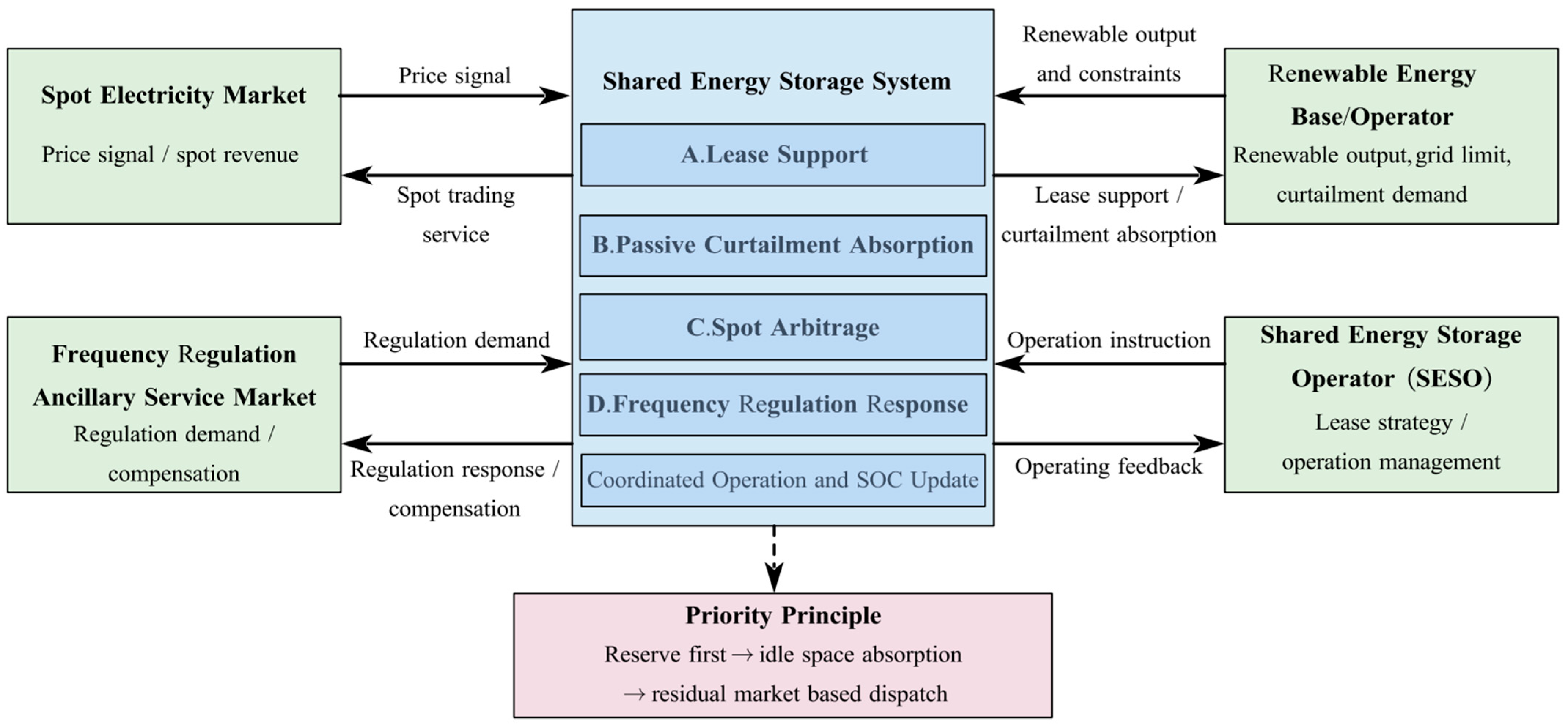
As shared energy storage shifts from single-function operation to joint multi-service operation, its capacity configuration and dispatch become more strongly coupled [9,10]. Leasing-based reliability support, passive accommodation of curtailed renewable energy, spot-market arbitrage, and frequency-regulation ancillary services occupy power capacity, energy capacity, and state-of-charge (SOC) space in different ways [11]. If service boundaries are not explicitly defined, reliability-support resources may be crowded out by market-oriented dispatch, and conflicts may arise among accommodation space, arbitrage space, and frequency-regulation reserves. Meanwhile, multi-service stacking increases cycling intensity and may accelerate battery degradation [12,13,14]. Capacity configuration models based on fixed-lifetime or static-depreciation assumptions may therefore overestimate the long-term economic performance of high-cycling operation schemes.
In summary, although existing studies have addressed the multi-scenario configuration and diversified revenue evaluation of shared energy storage, several limitations remain. First, the allocation of power-capacity space and service priorities among stacked services has not been clearly characterized, making it difficult to reflect resource-occupation boundaries in joint operation. Second, lifetime degradation is often treated using fixed depreciation periods or fixed cycling costs, without feeding actual operating intensity back into the economic lifetime and capacity-side depreciation cost. Third, the closed-loop mechanism among service boundaries, operating intensity, lifetime depreciation, and capacity configuration has not been sufficiently characterized [15,16]. Therefore, it remains difficult to jointly evaluate the effects of multi-service revenue improvement, curtailed-energy accommodation enhancement, and lifetime-depreciation cost variation on capacity configuration results.
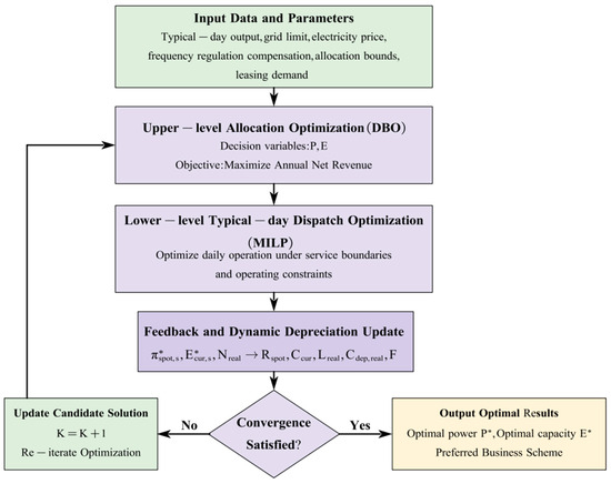
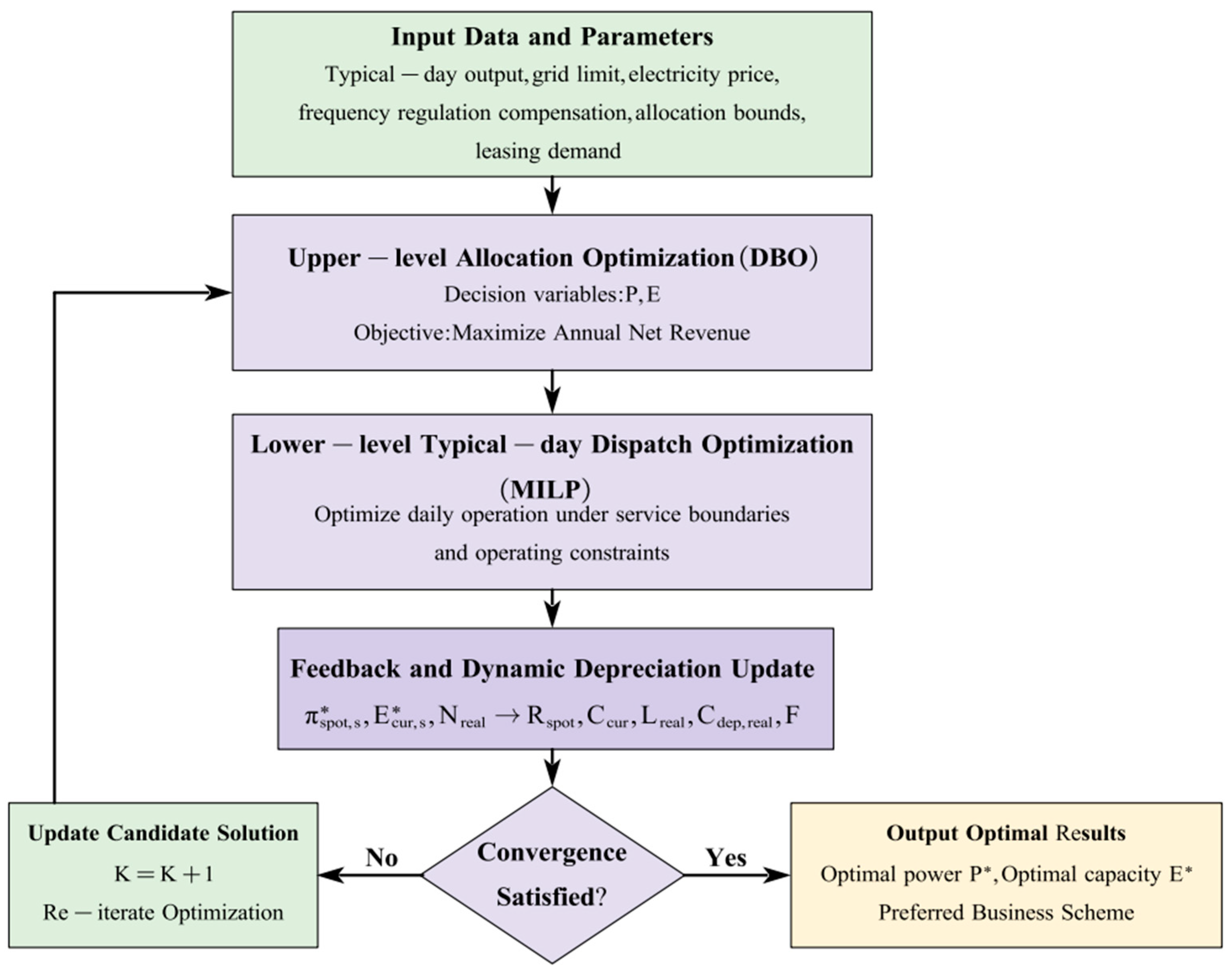
To address the above issues, this paper develops a bi-level optimal configuration method for shared energy storage in renewable energy bases under multi-service operation, considering operational intensity and dynamic depreciation. First, service-occupation boundaries and cycle-attribution rules are clarified under the principle of “reserve priority, idle-space accommodation, and residual market-based dispatch”. Second, annual equivalent cycles are used to quantify the operational intensity of shared energy storage and to connect service-specific cycling contributions with lifetime assessment. Third, operational intensity is fed back into the actual economic lifetime and capacity-side dynamic depreciation cost, forming a closed-loop capacity optimization framework solved by Dung Beetle Optimizer (DBO) and Mixed-integer linear programming (MILP) [17]. Seasonal representative-day case studies further verify the proposed method through dynamic-depreciation model comparison, multi-service scheme selection, operational-mechanism verification, and parameter sensitivity analysis. The results show that dynamic depreciation can correct the overestimation of high-cycling schemes and support economically robust multi-service operation decisions for shared energy storage in renewable energy bases. Compared with existing studies that mainly focus on shared energy storage scheduling, multi-service revenue evaluation, degradation-aware dispatch, or fixed cycling-cost representation, the present study further emphasizes the closed-loop interaction between service-boundary allocation, service-specific cycling intensity, economic lifetime correction, and capacity configuration. The methodological novelty of this paper therefore lies in the integration of four linked elements. First, the power-capacity, SOC-feasibility, and cycle-attribution boundaries of leasing-based reliability support, passive curtailed-energy accommodation, spot-market arbitrage, and frequency-regulation services are explicitly separated. Second, a service-specific cycle-attribution logic is established to avoid double counting of cycling contributions under multi-service stacking. Third, annual equivalent cycles are fed back into the actual economic lifetime and the annualized capacity-side dynamic depreciation cost, so that high-cycling configurations are economically corrected during capacity planning rather than only evaluated after dispatch. Finally, the above mechanisms are embedded into a bi-level configuration-dispatch framework, in which upper-level capacity decisions and lower-level representative-day operation interact through revenue, curtailed energy, cycling intensity, lifetime, and depreciation-cost feedback.
4. Case Study Setup and Verification of the Dynamic Depreciation Model
To verify the proposed shared energy storage capacity configuration model and the dynamic depreciation closed-loop mechanism, a case study is conducted using representative-day data from a renewable energy base. This section presents the data sources and parameter settings, and then verifies the model through depreciation comparison, business-scheme comparison, representative-day operation analysis, and market-parameter sensitivity analysis.
4.1. Data Sources and Parameter Settings
The case study uses data from a renewable energy base consisting of two wind farms and two photovoltaic power stations. The dispatch horizon is 24 h with a time resolution of 1 h, and the total installed capacity is 384 MW. Seasonal representative days are selected based on typicality indicators and converted into annualization weights according to the number of seasonal samples. The grid-connected power limit of each representative day is set as an exogenous boundary to characterize transmission constraints and potential curtailment risk, while the spot electricity price adopts a unified 24-point time-of-use sequence. Shared energy storage is located on the renewable energy base side and provides leasing-based reliability support, passive accommodation of curtailed renewable energy, spot-market arbitrage, and frequency-regulation ancillary services [34]. Its charging energy mainly comes from available renewable energy and curtailed-energy accommodation on the renewable energy side, without considering reverse charging from the external grid. The typicality evaluation results are provided in Table A1.
To improve the transparency of the representative-day construction, the selection procedure is further described as follows. The case study covers the full year of 2020 with an hourly resolution. The annual samples are first divided into four seasonal subsets, namely spring, summer, autumn, and winter. For each seasonal subset, candidate days are evaluated according to typicality indicators that reflect the renewable-output profile, the occurrence of grid-connection constraints, and the potential curtailed-energy risk. The day with the best overall representativeness is then selected as the representative day for the corresponding season. The probability coefficient in Table A1 denotes the normalized proportion of annual samples represented by each seasonal subset and is used as the annualization weight. The difference coefficient measures the normalized deviation between the selected representative day and the corresponding seasonal sample set. It is used to evaluate the representativeness of the selected day, rather than as an annualization weight. Therefore, the representative-day dispatch results are converted into annual values using the probability coefficients, while the difference coefficients are reported only to indicate the typicality of the selected scenarios.
To improve the reproducibility of the main case-study results, a simplified representative-day reproducibility dataset is provided as Supplementary Materials. This dataset includes the 24 h representative-day renewable-output profiles for spring, summer, autumn, and winter, the hourly grid-connection limits, the potential curtailed-energy profiles, the hourly spot-market price series, and the main parameter tables used in the optimization. The representative-day profiles are the direct inputs to the lower-level MILP dispatch model, while the economic parameters, engineering boundaries, and business-scheme settings are used in the upper-level capacity configuration and annualized economic evaluation.
The upper bounds of power and energy capacity in Table 1 are engineering planning boundaries rather than unconstrained optimization results. In the benchmark case, MW is determined by the grid-access capability, converter-capacity planning, and station-side installation feasibility of the renewable energy base. The corresponding upper energy-capacity bound MWh represents the maximum planned energy-storage scale under the benchmark engineering setting. Therefore, the optimized capacity results should be interpreted as optimal configurations under the specified access, investment, market, and engineering-boundary conditions.
To unify the economic evaluation criteria, the initial investment of shared energy storage is calculated as . Since the annualized net income F has already deducted the capacity-side annualized depreciation cost and the power-side annualized investment cost, the operating net cash flow is reconstructed as , where denotes the capacity-side annualized depreciation cost adopted in the evaluation model and denotes the power-side annualized investment cost. In the static depreciation model, is calculated using the fixed calendar life, whereas in the dynamic depreciation model it is taken as . These two annualized capital-cost terms are added back because they are accounting annualization items rather than actual annual operating cash outflows. The internal rate of return (IRR) is calculated by setting the net present value to zero, and the static payback period is calculated as . In the static depreciation model, the evaluation period is the calendar life; in the dynamic depreciation evaluation, it is the actual economic lifetime.
As shown in Table 1, the reference cycle life is 6000 cycles, and the calendar life is 15 years, corresponding to a lifetime transition threshold of 400 cycles/year. In subsequent schemes, P is close to 180 MW, and E reaches or approaches the upper limit, indicating that the optimized results are affected by the engineering configuration boundaries.
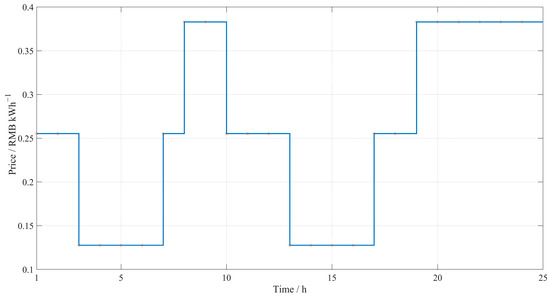
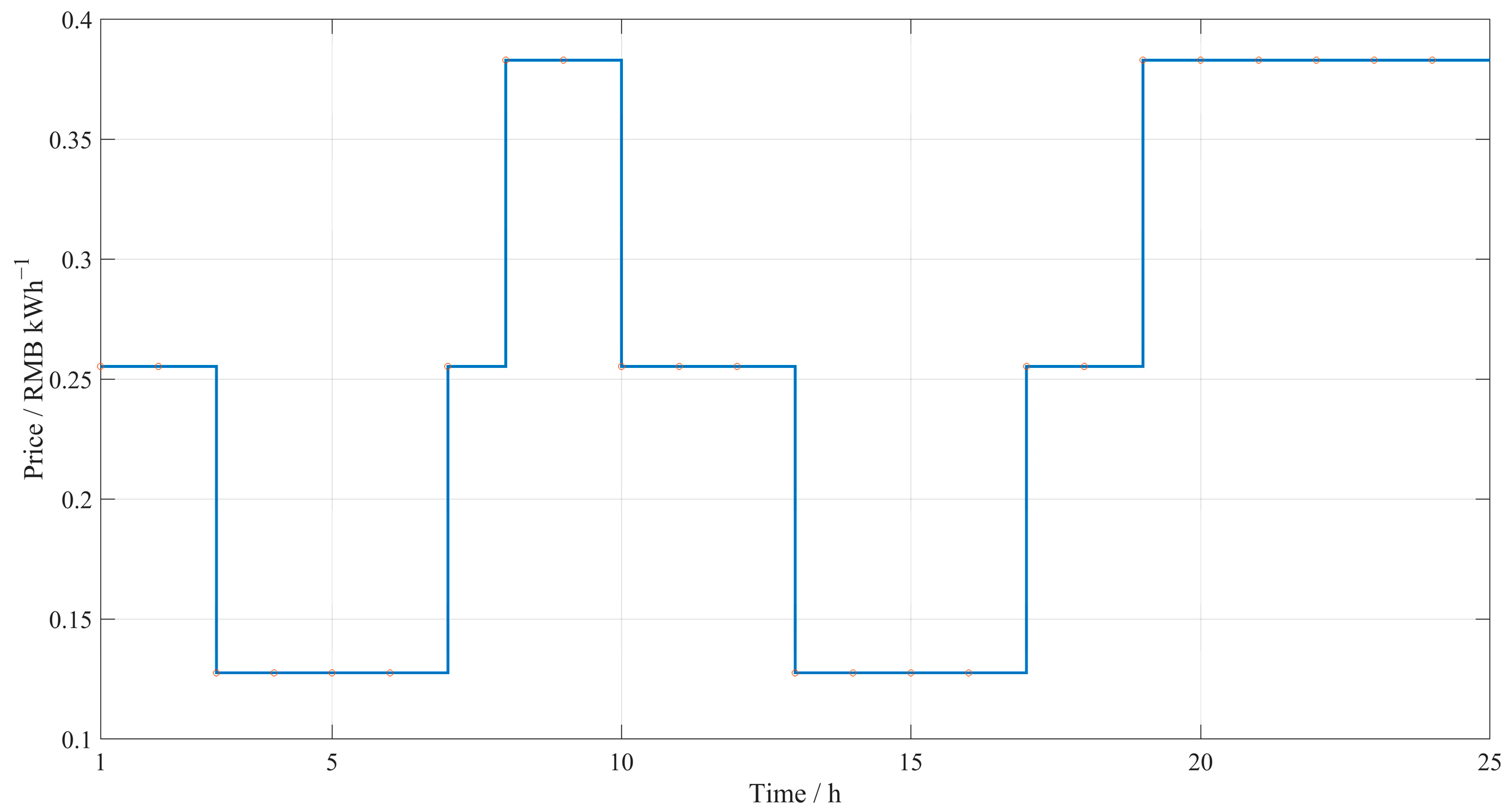
Figure 3 presents the 24 h electricity price curve. The peak-valley spread provides the price signal for spot-market arbitrage and the incentive for releasing SOC space at different times.
Figure 3.
Representative-day electricity price profile. The circular markers indicate hourly price-sampling points.
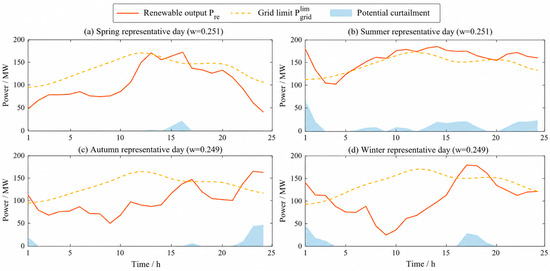
Figure 4 shows that renewable output exceeds the grid-connected power limit during some periods of all seasonal representative days, indicating the existence of curtailed-energy accommodation demand. The representative-day weights are provided in Table A1.
Figure 4.
Renewable energy output and grid-connected power limits of seasonal representative days.
4.2. Effectiveness Verification of the Dynamic Depreciation-Based Capacity Configuration Model
To examine the effect of dynamic depreciation, three depreciation treatments are compared under the S2 service boundary. M1 is the static depreciation model with a fixed 15-year battery lifetime. M2 keeps the M1 configuration unchanged but evaluates the actual lifetime and dynamic depreciation cost using annual equivalent cycles. M3 is the proposed dynamic-depreciation closed-loop model, in which operational cycles are fed back into lifetime assessment and depreciation-cost calculation during capacity optimization.
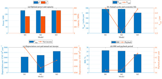
Table 2 gives the numerical comparison, while Figure 5 visualizes the relative differences among M1, M2, and M3.
Table 2.
Configuration, lifetime, and economic results under different depreciation models.
Figure 5.
Comparison of configuration, lifetime, and economic indicators under M1, M2, and M3.
As shown in Table 2 and Figure 5, M1 selects E* = 533 MWh and produces 476.71 cycles/year, exceeding the 400 cycles/year lifetime-transition threshold. Under the same configuration, M2 reduces the evaluated lifetime to 12.59 years, increases the capacity-side depreciation cost to 3436.46 × 104 CNY/year, and decreases annualized net income to 4274.93 × 104 CNY/year. This indicates that static depreciation overestimates the economic performance of high-cycling schemes. Compared with M2, M3 expands E* to 720 MWh, reduces to 403.04 cycles/year, restores the lifetime to 14.89 years, and increases annualized net income by 120.97 × 10⁴ CNY/year. Although its IRR is lower and payback period is longer due to the larger initial investment, M3 better reflects the trade-off among capacity scale, cycling intensity, lifetime degradation, and annualized income. The boundary values of P* and E* also indicate that the result should be interpreted as an optimum under the given access, cost, price, and capacity limits.
Although M1 and M2 have different evaluated lifetimes and annualized net incomes, their payback periods are the same because M2 is an ex post dynamic-depreciation evaluation of the M1 capacity configuration. Therefore, M1 and M2 share the same P*/E* configuration, initial investment, and representative-day dispatch results. The payback period is calculated according to the recovery of the initial investment by operating cash flows, rather than by the accounting annualized depreciation cost. Consequently, the dynamic lifetime correction in M2 changes the annualized depreciation cost and annualized net income, but it does not change the cash-flow recovery process under the same configuration and dispatch.
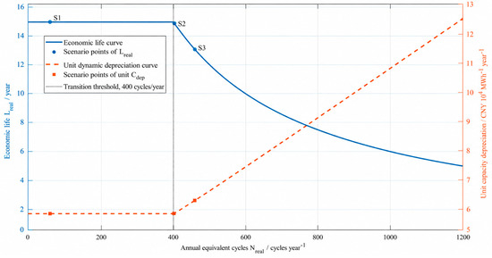
Figure 6 explains the mechanism behind Table 2: once annual equivalent cycles exceed 400 cycles/year, economic lifetime declines and unit capacity-side dynamic depreciation cost increases, converting operational intensity into a cost signal for capacity configuration.
Figure 6.
Relationship among annual equivalent cycles, economic lifetime, and unit capacity-side dynamic depreciation cost.
4.3. Economic Operation Analysis of Shared Energy Storage Under Different Business Schemes
Three business schemes are compared. S1 includes leasing-based reliability support and passive accommodation of curtailed renewable energy. S2 adds spot-market arbitrage to S1, while S3 further incorporates frequency-regulation ancillary services. For all schemes, the capacity configuration is re-optimized under the corresponding service boundaries, and the detailed settings are provided in Table A2. The parameter settings of S1, S2, and S3 are not intended to represent a purely additive revenue comparison with all boundary parameters fixed. Instead, they are designed to represent three feasible business-boundary scenarios under the priority principle of “reserve first, idle-space accommodation, and residual market-based dispatch”. Specifically, S1 represents a leasing-dominated operation mode, in which a relatively larger proportion of power capacity is reserved for reliability support and only idle leased resources are used for passively curtailed-energy accommodation. S2 introduces spot-market arbitrage and therefore retains part of the converter capacity as arbitrage-available power after satisfying the leasing boundary. S3 further reserves part of the converter capacity for frequency-regulation services, which reduces the power space available for arbitrage and changes the cycling-intensity level. The corresponding leasing reserve ratios, frequency-regulation reserve ratio, and maintenance-cycle assumptions are reported in Table A3 and are used to define internally consistent service-boundary scenarios rather than isolated service additions.
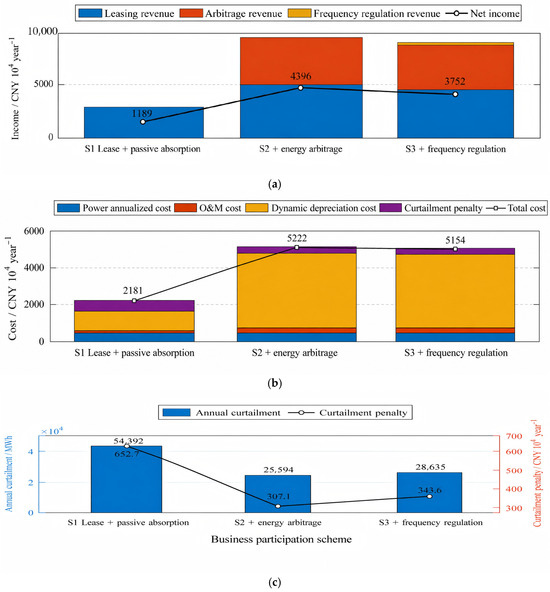
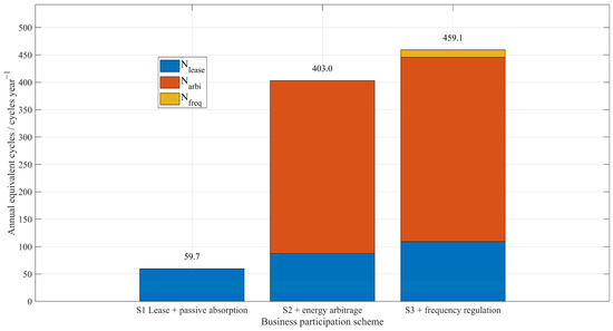
Table 3 summarizes the cycling, lifetime, and net-income results; Figure 7 further presents the economic-performance comparison from three aspects, including revenue composition and annual net income, cost composition and total annual cost, and annual curtailment and curtailment penalty; Figure 8 separates the cycle sources.
Table 3.
Cycling, lifetime, and economic results under different business schemes.
Figure 7.
Economic-performance comparison under different business participation schemes: (a) revenue composition and annual net income; (b) cost composition and total annual cost; (c) annual curtailment and curtailment penalty.
Figure 8.
Composition of annual equivalent cycle sources under different business schemes.
As shown in Table 3 and Figure 7a, S1 obtains 1188.98 × 104 CNY/year of annualized net income with only 59.70 cycles/year. After spot-market arbitrage is introduced in S2, increases to 315.69 cycles/year, and the annualized net income rises to 4395.90 × 104 CNY/year. Figure 7b shows that the total annual cost also increases because the larger optimized capacity and higher multi-service cycling intensity raise the dynamic depreciation cost. Figure 7c further shows that annual curtailment decreases from 54,392 MWh in S1 to 25,594 MWh in S2, indicating that the combination of passive accommodation and spot-market arbitrage improves SOC-space utilization and curtailed-energy accommodation. Although S3 gains frequency-regulation revenue, frequency-regulation reserves occupy part of the adjustable power capacity and increase to 459.08 cycles/year, reducing to 13.07 years and making its annualized net income lower than that of S2 under the benchmark compensation level. Therefore, S2 is selected as the preferred scheme under the benchmark conditions.
It should be emphasized that the comparison among S1, S2, and S3 reflects the combined effects of service addition and service-boundary settings. The increase in annualized net income from S1 to S2 is mainly related to the introduction of spot-market arbitrage and the improved use of SOC space for passive accommodation. However, it is also affected by the adjusted leasing boundary and maintenance-cycle assumptions. Similarly, the lower annualized net income of S3 under the benchmark compensation level is not caused by frequency-regulation participation alone, but by the combined effect of frequency-regulation revenue, reserve-capacity occupation, reduced arbitrage-available power, increased cycling intensity, and higher dynamic depreciation pressure.
Figure 8 further shows that the increase in S2 mainly comes from price-driven arbitrage cycles, whereas the additional cycles in S3 include the frequency-regulation component. This supports the conclusion that scheme selection should consider both revenue increments and dynamic depreciation costs.
4.4. Verification of Representative-Day Dispatch Strategy and Operating Mechanism
To explain the operating mechanisms of different business schemes, the spring representative day of 26 April 2020 is selected to analyze power allocation, SOC variation, and curtailed-energy accommodation. These results illustrate representative-day operation, while annualized economic performance is still evaluated using the weighted results of four seasonal representative days.
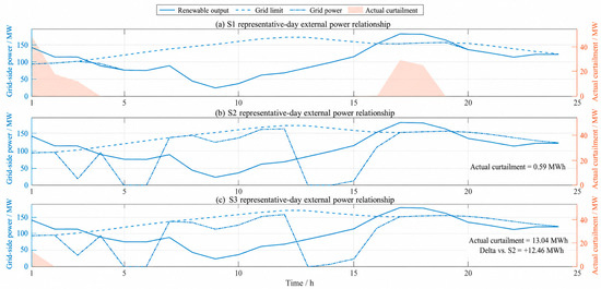
Figure 9 and Figure 10 describe the dispatch process from external power balance and internal storage allocation, respectively; Table 4 then summarizes the corresponding accommodation and arbitrage statistics. The corresponding SOC trajectories under different business schemes are provided in Figure A1.
Figure 9.
External power relationships of S1, S2, and S3 on the representative day.
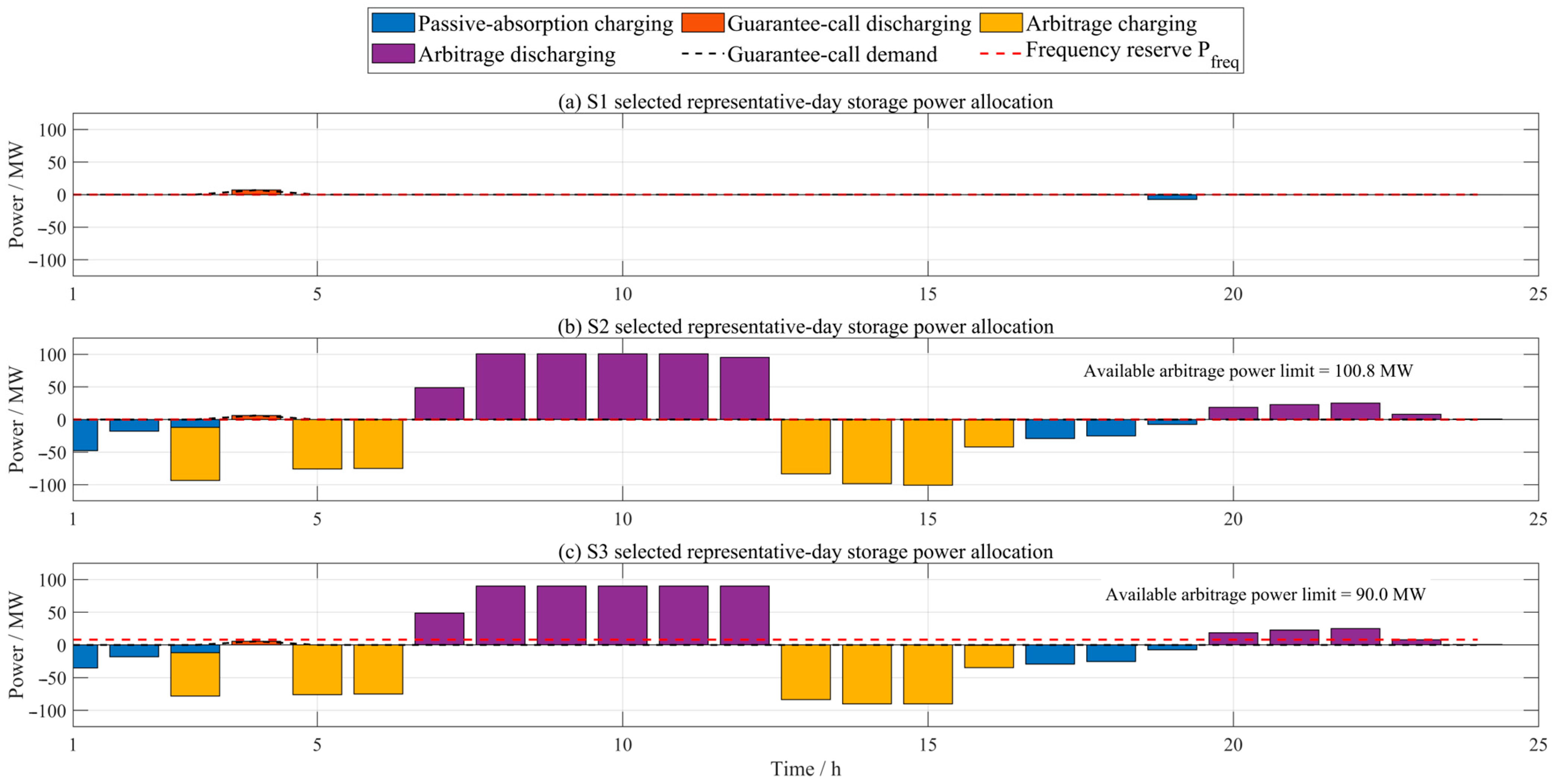
Figure 10.
Energy storage power allocation of S1, S2, and S3 on the representative day.
Table 4.
Representative-day curtailed-energy accommodation and arbitrage dispatch results.
Figure 9 shows the external relationship among renewable output, grid-connection limits, curtailed energy, and grid-connected power.
Figure 10 decomposes the internal power allocation of shared energy storage under the three schemes, explaining the operational source of the differences observed in Figure 9.
As shown in Figure 9 and Figure 10 and Table 4, the actual curtailed energy in S1 is 132.66 MWh. In S2, arbitrage discharging releases SOC space, increasing passive accommodation to 139.86 MWh and reducing actual curtailment to 0.59 MWh. In S3, frequency-regulation reserves reduce the available dispatch space, decreasing passive accommodation to 127.40 MWh and increasing actual curtailment to 13.04 MWh. The arbitrage charging and discharging values in Table 4 are statistical results of the arbitrage power channel and do not form an independent energy-closure relationship; the overall energy balance is governed by the SOC dynamic equation and the initial-terminal SOC closure constraint in Equation (23).
The charging and discharging quantities reported in Table 4 are channel-specific statistical quantities used for revenue calculation and cycle attribution. They do not imply that each service channel must be independently energy balanced. The physical energy balance of the shared energy storage system is enforced at the system level by the SOC dynamic constraint, SOC upper and lower limits, and the initial-terminal SOC closure condition. As shown by the SOC trajectories in Figure A1, the SOC remains within the allowable range and returns to the specified terminal level for each representative day. Therefore, the channel-specific statistics in Table 4 should be interpreted together with the SOC trajectories in Figure A1.
4.5. Verification of Key Mechanisms and Sensitivity Analysis
4.5.1. Verification of the Passive Curtailed-Energy Accommodation Mechanism
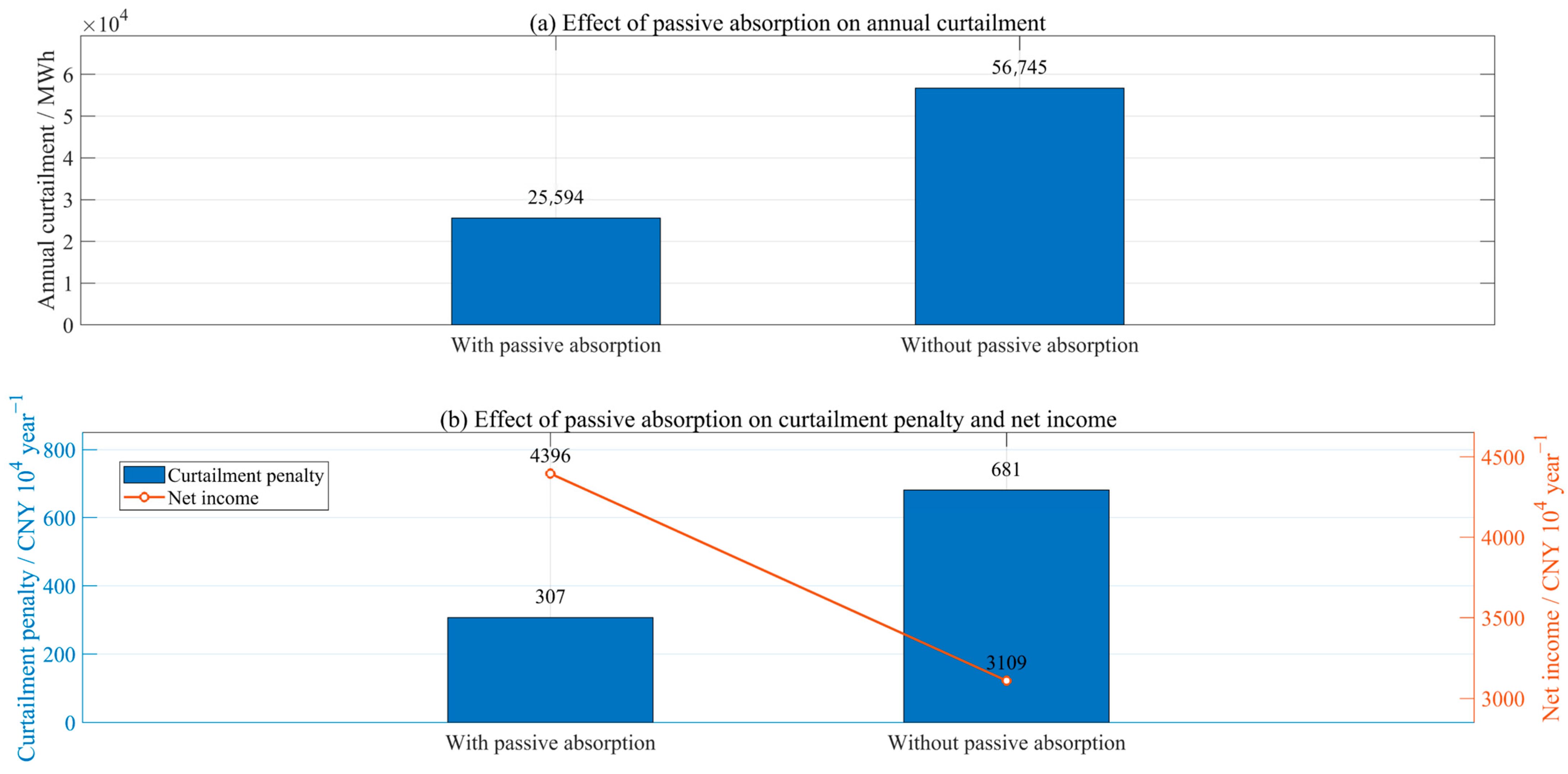
To verify the role of passive curtailed-energy accommodation, S2 is used as the benchmark, the passive accommodation function is disabled, and the capacity configuration is then re-optimized. As shown in Figure 11, disabling passive accommodation increases annual curtailed energy from 25,594.30 MWh to 56,744.74 MWh and decreases annualized net income from 4395.90 × 104 CNY to 3108.88 × 104 CNY. Therefore, passive accommodation improves economic performance by reducing curtailment penalties and utilizing idle leased resources, and its cycling contribution should be attributed to leasing-related cycles rather than spot-market arbitrage cycles [35].
Figure 11.
Ablation analysis of the passive curtailed-energy accommodation mechanism.
4.5.2. Market Parameter Sensitivity and Preferred Business Scheme
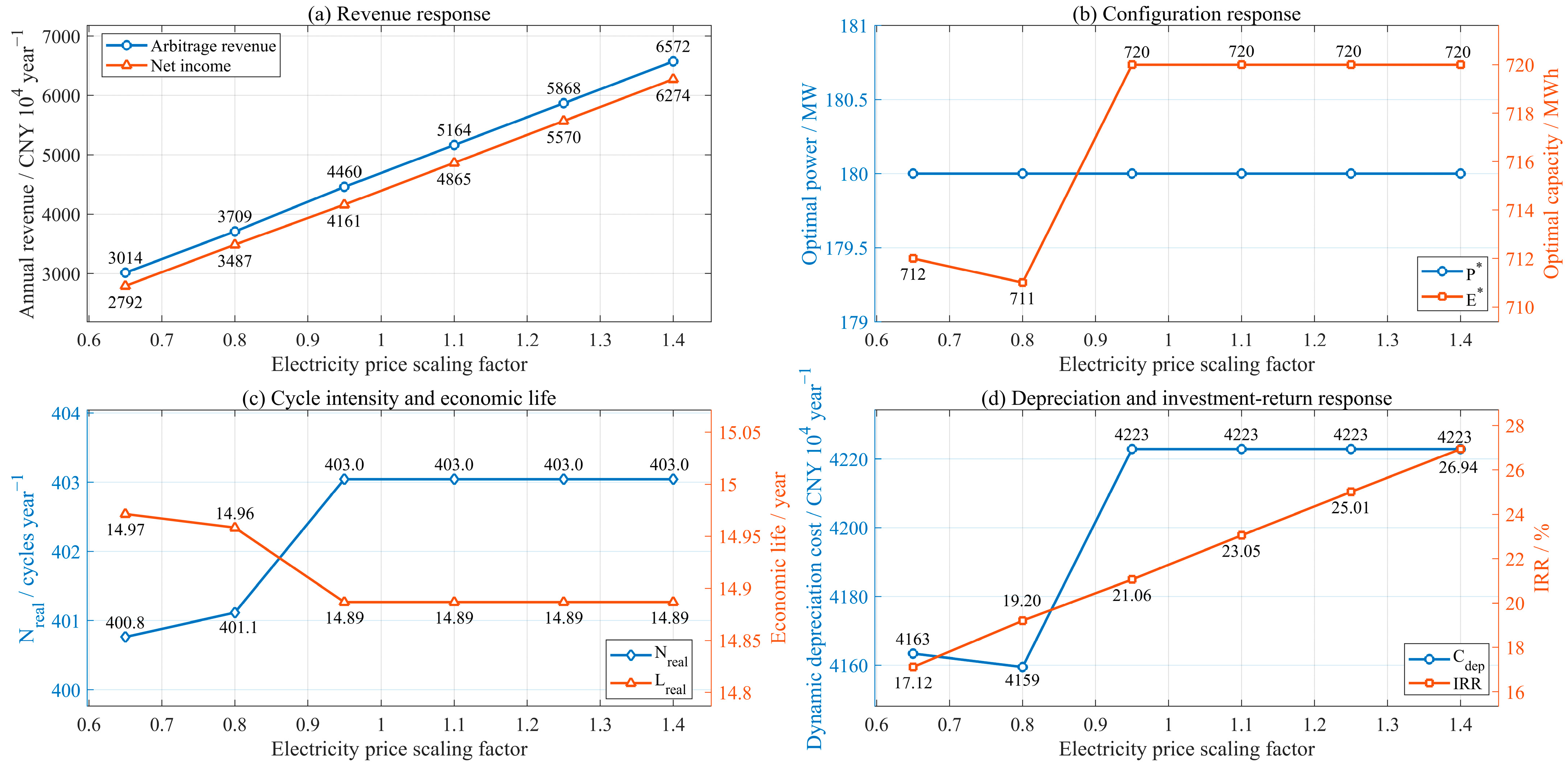
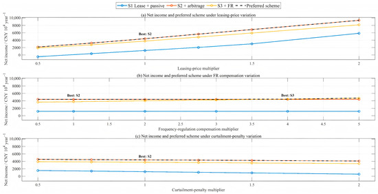
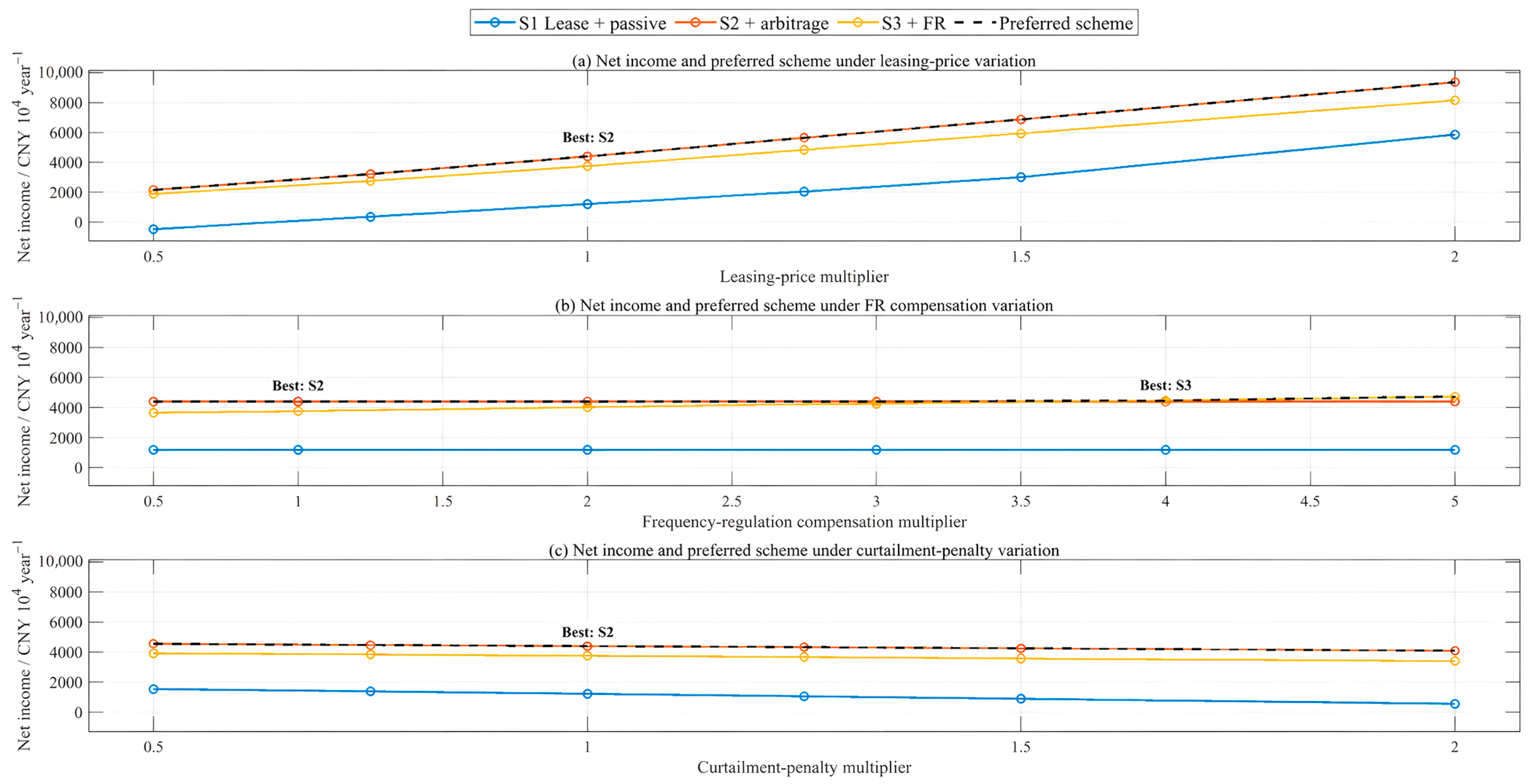
To examine parameter robustness, sensitivity analyses are conducted on electricity price scaling, unit leasing prices, and frequency-regulation compensation. The proposed depreciation mechanism should be interpreted as an economic planning model based on annual equivalent cycles, rather than as a full electrochemical battery degradation model, and curtailed-energy penalty. The electricity price scaling results are reported in Table 5 and Figure A2, while the sensitivity results for unit leasing prices, frequency-regulation compensation, and curtailed-energy penalty are shown in Figure 12 and Table 5.
Table 5.
Market parameter sensitivity analysis results.
Figure 12.
Sensitivity of unit leasing price, frequency-regulation compensation, and curtailed-energy penalty, and the preferred business scheme.
Figure 12 shows the sensitivity trends, and Table 5 provides the corresponding low- and high-value endpoint results.
As shown in Figure 12 and Table 5, increasing the electricity price scaling factor from 0.65 to 1.40 raises annualized net income from 2791 × 104 CNY/year to 6274 × 104 CNY/year and increases the optimal energy capacity from 707 MWh to 720 MWh, indicating that electricity price mainly affects arbitrage revenue and boundary utilization. Under variations in unit leasing prices and curtailed-energy penalty, S2 remains preferred.
To further identify the economic switching point between S2 and S3, a refined sweep of the frequency-regulation compensation multiplier was conducted around the transition region. As shown in Table A6, S2 remains preferable when ,whereas S3 becomes preferable from under the adopted 0.05 scanning resolution. Linear interpolation between and gives an estimated switching threshold of . Therefore, under the benchmark service-boundary and dynamic-depreciation assumptions, S3 becomes economically preferable only when the frequency-regulation compensation level increases to approximately 3.68 times the benchmark value. Below this threshold, the additional frequency-regulation revenue cannot offset reserve-capacity occupation, reduced arbitrage-available power, increased cycling intensity, and higher dynamic depreciation pressure.
4.5.3. Capacity-Boundary Sensitivity Analysis
In the benchmark M3 and S2 results, the optimized energy capacity reaches the imposed upper bound of 720 MWh. To further examine whether this result is mainly restricted by the upper energy-capacity boundary, an additional sensitivity test is conducted by expanding from 720 MWh to 840 MWh and 960 MWh, while keeping the power-capacity upper bound, market parameters, grid-connection constraints, and service-boundary settings unchanged. Since the model also imposes an upper limit on the E/P ratio, the E/P upper bound is relaxed consistently with the expanded to avoid retaining the original 4 h duration boundary.
As shown in Table 6, when is increased from 720 MWh to 840 MWh, the optimized energy capacity increases only slightly from 720 MWh to 728 MWh, and the annualized net income increases from 4395.90 × 104 CNY/year to 4400.79 × 104 CNY/year, corresponding to an increase of approximately 0.11%. When is further increased to 960 MWh, the optimized configuration and annualized net income remain unchanged. These results indicate that the benchmark solution is affected by the imposed energy-capacity boundary, but the marginal economic benefit of further expanding the energy capacity is very limited. Therefore, the benchmark M3 result should be interpreted as a boundary-conditioned optimum close to the economic saturation region under the given market, grid-connection, service-boundary, and dynamic-depreciation assumptions. It should also be noted that the optimized power capacity remains at the upper bound of 180 MW, indicating that the result is still conditioned by the engineering power-access boundary.
Table 6.
Sensitivity of the optimized M3 configuration to the upper energy-capacity bound.
4.6. Applicability and Limitations of the Proposed Model
The proposed model is most applicable to renewable energy bases where shared energy storage simultaneously provides leasing-based reliability support, passive curtailed-energy accommodation, spot-market arbitrage, and frequency-regulation reserve under clearly defined service boundaries. The representative-day reduction is appropriate when the selected seasonal profiles can adequately capture renewable-output patterns, grid-connection constraints, and curtailed-energy risk characteristics of the annual samples. Under these conditions, the model can evaluate how service-boundary allocation and cycling intensity affect capacity configuration, economic lifetime, dynamic depreciation cost, and annualized net income.
The model may become less reliable when actual operation deviates from the benchmark assumptions. First, if extreme renewable-output events or grid-connection restrictions are not represented by the selected typical days, the annual revenue, curtailed-energy reduction, and cycling-intensity evaluation may be biased. Second, if market rules or contractual arrangements allow the service boundaries to be dynamically redefined, for example, if passive accommodation becomes an independently priced service or frequency-regulation reserve is co-optimized with energy arbitrage at a higher time resolution, the boundary parameters should be recalibrated. Third, the current frequency-regulation treatment assumes an approximately zero-mean response at the day-ahead dispatch timescale; persistent regulation-energy bias or high-resolution regulation trajectories with nonzero cumulative energy should be explicitly incorporated into the SOC dynamics. Fourth, the dynamic depreciation mechanism is a planning-level economic depreciation model based on annual equivalent cycles. It does not explicitly capture temperature dependence, C-rate effects, variable depth-of-discharge ageing, SOC-dependent calendar ageing, or state-of-health-dependent capacity fade. Therefore, applications requiring detailed battery-health prediction should replace or extend the equivalent-cycle-based lifetime function with a more detailed degradation model. Finally, the optimized capacity and preferred business scheme remain conditional on market prices, compensation levels, grid-connection limits, and configuration boundaries. Cross-regional applications should therefore recalibrate these parameters and, when necessary, repeat the market-parameter and capacity-boundary sensitivity analyses.
5. Conclusions
Based on representative-day data from a renewable energy base, this paper verifies the shared energy storage capacity configuration model, the dynamic-depreciation closed-loop mechanism, and the multi-service operation strategy through a case study. The main conclusions are as follows.
(1) The dynamic-depreciation closed-loop mechanism can correct the overestimation of the economic performance of high-cycling schemes caused by static depreciation. The ex post dynamic evaluation in M2 shows that, for the M1 configuration, the actual economic lifetime decreases to 12.59 years and the annualized net income decreases to 4274.93 × 104 CNY. Through cycle feedback, M3 increases the energy capacity from 533 MWh to 720 MWh, reduces the annual equivalent number of cycles to 403.04 cycles/year, and achieves a higher annualized net income than M2. Although its annualized net income is lower than the static-depreciation estimate in M1, M3 provides a more realistic evaluation by incorporating the impact of operational intensity on lifetime and capacity-side depreciation.
(2) Under the benchmark parameters, S2 achieves the highest annualized net income, indicating that “leasing-based reliability support + passive accommodation + spot-market arbitrage” provides a better balance among revenue improvement, SOC-space utilization, and lifetime degradation. The selected spring representative day further shows that S2 coordinates price-driven arbitrage and passive accommodation by releasing SOC space before high-curtailment-risk periods and using idle leased resources for curtailed-energy accommodation. As a result, the potential curtailed-energy accommodation rate of this representative day increases from 5.54% in S1 to 99.59% in S2.
(3) The passive-accommodation disabling test and sensitivity analysis show that passive accommodation plays an important role in reducing curtailed-energy penalties and improving annualized net income. Under variations in electricity price scaling, unit leasing prices, and curtailed-energy penalties, S2 maintains strong stability. When frequency-regulation compensation becomes high enough to offset the additional cycling degradation and dynamic-depreciation pressure, the preferred scheme may switch from S2 to S3. This indicates that the proposed model can identify the switching boundary of business strategies under different market compensation conditions.
It should be noted that the optimal configuration and preferred business scheme obtained in this paper are closely related to renewable energy output characteristics, grid-connection constraints, market prices, frequency-regulation compensation levels, and configuration boundary conditions. Therefore, they should not be directly interpreted as general capacity recommendations for all renewable energy bases. The main contribution of this paper is to establish an analytical framework that couples service boundaries, operational intensity, cycle-intensity-adjusted economic depreciation, and capacity configuration. The proposed depreciation mechanism should therefore be interpreted as a planning-level economic depreciation model based on annual equivalent cycles, rather than as a full electrochemical battery degradation model. Future research can further incorporate higher-resolution frequency-regulation response signals, more detailed state-of-health degradation models considering temperature, C-rate, variable depth-of-discharge ageing, and SOC-dependent calendar ageing, as well as broader cross-regional validation under different market mechanisms, grid-connection constraints, and planning-boundary assumptions.
Supplementary Materials
The following supporting information can be downloaded at: https://www.mdpi.com/article/10.3390/en19143311/s1, Supplementary Materials provides a simplified representative-day reproducibility dataset, covering seasonal representative-day renewable-output profiles, grid-connection limits, potential curtailed-energy profiles, spot-market price series, common parameter settings, and business-scheme settings.
Author Contributions
Conceptualization, Y.W., M.H. and T.X.; methodology, Y.W.; software, Y.W.; validation, Y.W., J.Z. and P.L.; investigation, Y.W.; resources, M.H. and T.X.; data curation, Y.W.; writing—original draft preparation, Y.W.; writing—review and editing, Y.W., J.Z., P.L., M.H. and T.X.; visualization, Y.W.; supervision, M.H. and T.X. All authors have read and agreed to the published version of the manuscript.
Funding
This research was funded by the Yunnan Provincial Science and Technology Talents and Platform Program, grant number 202105AD160042.
Data Availability Statement
The simplified representative-day reproducibility dataset and parameter tables used to reproduce the main case-study results are provided in Supplementary Materials. The original full-year renewable-energy output data, grid-connection constraint data, and part of the raw market-parameter data are available from the corresponding author upon reasonable request. Some raw project and third-party data are not publicly available due to project confidentiality and third-party data restrictions.
Conflicts of Interest
The authors declare no conflicts of interest.
Abbreviations
| Symbol | Definition |
| SES | Shared energy storage |
| DBO | Dung Beetle Optimizer |
| MILP | Mixed-integer linear programming |
| IRR | Internal rate of return |
| S1 | Leasing-based reliability support + passive accommodation of curtailed renewable energy |
| S2 | Leasing-based reliability support + passive accommodation of curtailed renewable energy + spot-market arbitrage |
| S3 | Leasing-based reliability support + passive accommodation of curtailed renewable energy + spot-market arbitrage + frequency-regulation ancillary services |
| M1 | Static depreciation model |
| M2 | Ex post dynamic depreciation evaluation model under a fixed configuration |
| M3 | Dynamic depreciation closed-loop optimization model |
| P | Rated power of shared energy storage |
| E | Rated energy capacity of shared energy storage |
| Annual equivalent number of cycles | |
| Actual economic lifetime | |
| Capacity-side dynamic depreciation cost | |
| Annual leasing revenue | |
| Annual spot-market arbitrage revenue | |
| Annual revenue from frequency-regulation ancillary services | |
| Annualized curtailed-energy penalty cost |
Appendix A
Appendix A provides supplementary information supporting the case study and sensitivity analysis, including the typicality indicators of seasonal representative days, the settings of comparative models and business schemes, the service-reservation and supplementary-constraint parameters, representative-day SOC trajectories, and electricity-price-scaling sensitivity results.
Table A1.
Probability coefficients and difference coefficients of seasonal typical scenarios.
Table A2.
Business boundaries and main results of comparative cases.
Table A3.
Parameter settings for service reservation and supplementary constraints.
To support computational reproducibility, the detailed implementation settings of the DBO–MILP solution procedure are provided in Table A4.
Table A4.
Computational implementation settings of the DBO–MILP solution procedure.
To evaluate the stability of the metaheuristic upper-level search, the benchmark M3 case was repeated for 10 independent DBO runs with different random seeds, and the results are reported in Table A5.
Table A5.
Independent-run stability of the upper-level DBO search.
Table A6.
Refined threshold analysis of the frequency-regulation compensation multiplier.
Figure A1.
Representative-day SOC trajectories under different business schemes.
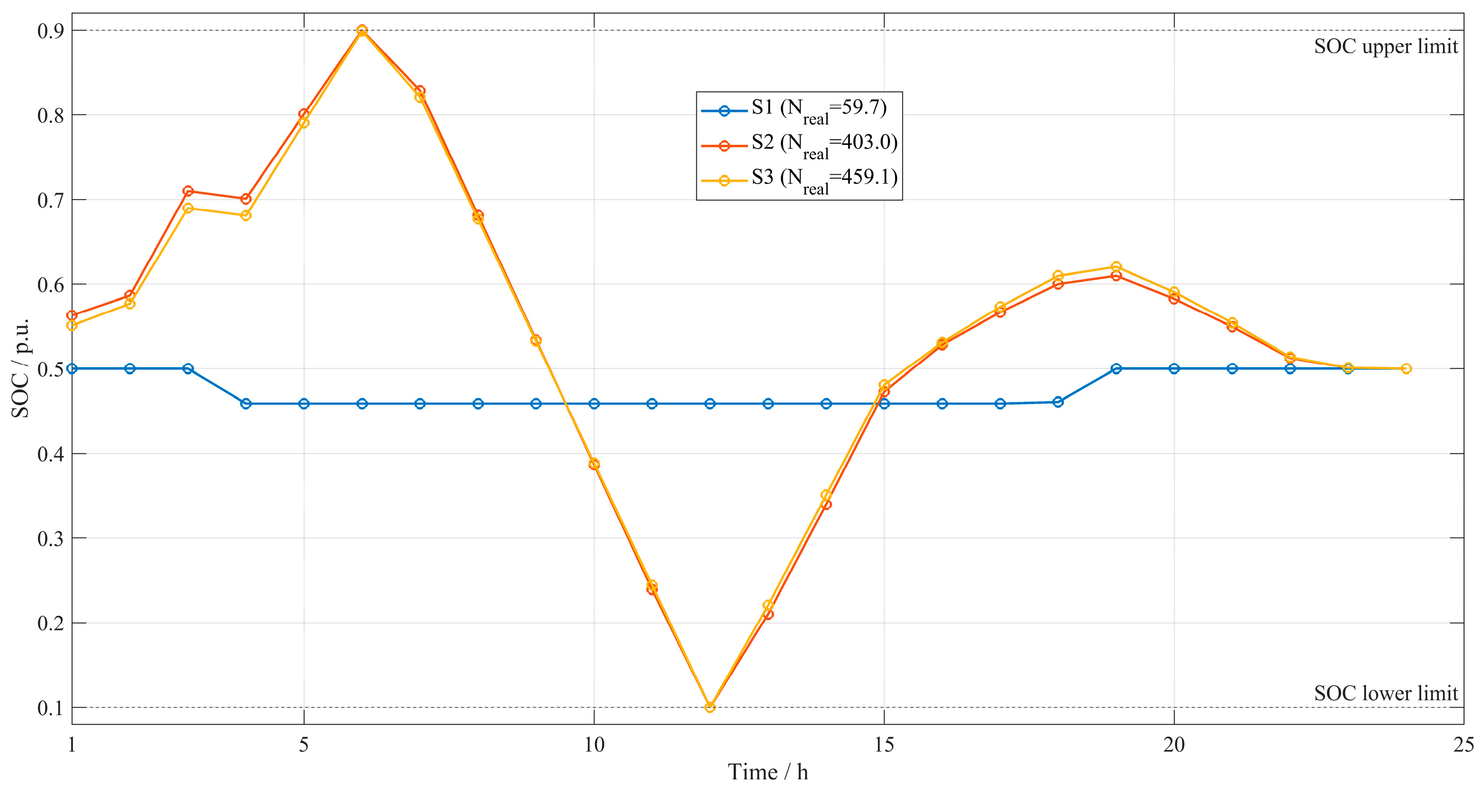
Figure A2.
Effects of electricity price scaling on revenue, configuration, cycle life, and investment return.
References
- Sayed, E.T.; Olabi, A.G.; Alami, A.H.; Radwan, A.; Mdallal, A.; Rezk, A.; Abdelkareem, M.A. Renewable Energy and Energy Storage Systems. Energies 2023, 16, 1415. [Google Scholar] [CrossRef] [Scilit]
- Yuan, Z.; He, Y.; Meng, Z. Hybrid energy storage configuration methodology, taking into account the accumulation of wind farm forecast deviations. Front. Energy Res. 2024, 12, 1343879. [Google Scholar] [CrossRef] [Scilit]
- Jafari, M.; Korpås, M.; Botterud, A. Power system decarbonization: Impacts of energy storage duration and interannual renewables variability. Renew. Energy 2020, 156, 1171–1185. [Google Scholar] [CrossRef] [Scilit]
- Qiu, W.; Zhou, S.; Yang, Y.; Lv, X.; Lv, T.; Chen, Y.; Huang, Y.; Zhang, K.; Yu, H.; Wang, Y.; et al. Application Prospect, Development Status and Key Technologies of Shared Energy Storage toward Renewable Energy Accommodation Scenario in the Context of China. Energies 2023, 16, 731. [Google Scholar] [CrossRef] [Scilit]
- Xiao, J.-W.; Yang, Y.-B.; Cui, S.; Liu, X.-K. A new energy storage sharing framework with regard to both storage capacity and power capacity. Appl. Energy 2022, 307, 118171. [Google Scholar] [CrossRef] [Scilit]
- Khojasteh, M.; Faria, P.; Gomes, L.; Vale, Z. Energy trading strategy of community shared energy storage. Electr. Eng. 2024, 106, 3415–3426. [Google Scholar] [CrossRef] [Scilit]
- Li, L.; Cao, X.; Zhang, S. Shared energy storage system for prosumers in a community: Investment decision, economic operation, and benefits allocation under a cost-effective way. J. Energy Storage 2022, 50, 104710. [Google Scholar] [CrossRef] [Scilit]
- Han, O.; Ding, T.; Zhang, X.; Mu, C.; He, X.; Zhang, H.; Jia, W.; Ma, Z. A shared energy storage business model for data center clusters considering renewable energy uncertainties. Renew. Energy 2023, 202, 1273–1290. [Google Scholar] [CrossRef] [Scilit]
- He, Y.; Xiao, J.-W.; Wang, Y.-W.; Liu, Z.-W.; He, S.-Y. Subjective-uncertainty-oriented dynamic renting framework for energy storage sharing. Appl. Energy 2025, 378, 124765. [Google Scholar] [CrossRef] [Scilit]
- Lan, Z.; Hu, J.; Fang, X.; Qiu, W.; Li, J. Risk-based optimization for facilitating the leasing services of shared energy storage among renewable energy stations. Front. Energy Res. 2023, 11, 1286045. [Google Scholar] [CrossRef] [Scilit]
- Liu, J.; Wu, J.; Lei, Z. Two-Stage Optimization Strategy for Market-Oriented Lease of Shared Energy Storage in Wind Farm Clusters. Energies 2025, 18, 2697. [Google Scholar] [CrossRef] [Scilit]
- Miao, Y.; Chen, T.; Bu, S.; Liang, H.; Han, Z. Co-Optimizing Battery Storage for Energy Arbitrage and Frequency Regulation in Real-Time Markets Using Deep Reinforcement Learning. Energies 2021, 14, 8365. [Google Scholar] [CrossRef] [Scilit]
- Pusceddu, E.; Zakeri, B.; Castagneto Gissey, G. Synergies between Energy Arbitrage and Fast Frequency Response for Battery Energy Storage Systems. Appl. Energy 2021, 283, 116274. [Google Scholar] [CrossRef] [Scilit]
- Ellis, B.; White, C.; Swan, L. Degradation of Lithium-Ion Batteries That Are Simultaneously Servicing Energy Arbitrage and Frequency Regulation Markets. J. Energy Storage 2023, 66, 107409. [Google Scholar] [CrossRef] [Scilit]
- Lee, J.-O.; Kim, Y.-S. Novel Battery Degradation Cost Formulation for Optimal Scheduling of Battery Energy Storage Systems. Int. J. Electr. Power Energy Syst. 2022, 137, 107795. [Google Scholar] [CrossRef] [Scilit]
- Amini, M.; Khorsandi, A.; Vahidi, B.; Hosseinian, S.H.; Malakmahmoudi, A. Optimal Sizing of Battery Energy Storage in a Microgrid Considering Capacity Degradation and Replacement Year. Electr. Power Syst. Res. 2021, 195, 107170. [Google Scholar] [CrossRef] [Scilit]
- Xue, J.; Shen, B. Dung Beetle Optimizer: A New Meta-Heuristic Algorithm for Global Optimization. J. Supercomput. 2023, 79, 7305–7336. [Google Scholar] [CrossRef] [Scilit]
- Dou, Q.; Gao, X.; Wu, Y.; Chen, Y.; Xie, R.; Chen, J. A Multi-Level Coordinated Scheduling Strategy for Shared Energy Storage Systems under Electricity Spot and Ancillary Service Markets. IET Renew. Power Gener. 2024, 18, 3855–3868. [Google Scholar] [CrossRef] [Scilit]
- Wang, Z.; Yang, S.; Xue, F.; Tan, Z.; Liu, W.; Ju, L. Robust Two-Level Market Coordinated Transaction Optimal Model and Benefit Allocation Strategy for a Novel Shared-Energy Aggregator. IET Renew. Power Gener. 2024, 18, 1535–1555. [Google Scholar] [CrossRef] [Scilit]
- Yang, Y.; Chen, T.; Yan, H.; Wang, J.; Yan, Z.; Liu, W. Optimization Operation Strategy for Shared Energy Storage and Regional Integrated Energy Systems Based on Multi-Level Game. Energies 2024, 17, 1770. [Google Scholar] [CrossRef] [Scilit]
- Cui, K.; Fan, K.; Zhao, Y.; Chi, M. Decentralized Micro-Energy Storage Capacity Sharing within the Residential Community: An Enhanced Uniform Price-Based Bidding Framework. Front. Energy Res. 2024, 12, 1409444. [Google Scholar] [CrossRef] [Scilit]
- Wang, W.; Wang, H.; Sun, S.; Cao, G.; Wang, S.; Ji, Y. Optimal Configuration of Shared Energy Storage for Industrial Users Considering Lifetime and Charge-Discharge Strategy Coupling. Front. Energy Res. 2024, 12, 1510259. [Google Scholar] [CrossRef] [Scilit]
- Zhang, L.; Yu, Y.; Li, B.; Qian, X.; Zhang, S.; Wang, X.; Zhang, X.; Chen, M. Improved Cycle Aging Cost Model for Battery Energy Storage Systems Considering More Accurate Battery Life Degradation. IEEE Access 2022, 10, 297–307. [Google Scholar] [CrossRef] [Scilit]
- Collath, N.; Cornejo, M.; Engwerth, V.; Hesse, H.; Jossen, A. Increasing the Lifetime Profitability of Battery Energy Storage Systems through Aging Aware Operation. Appl. Energy 2023, 348, 121531. [Google Scholar] [CrossRef] [Scilit]
- He, G.; Ciez, R.E.; Moutis, P.; Kar, S.; Whitacre, J.F. The Economic End of Life of Electrochemical Energy Storage. Appl. Energy 2020, 273, 115151. [Google Scholar] [CrossRef] [Scilit]
- Mostafa, M.H.; Abdel Aleem, S.H.E.; Ali, S.G.; Ali, Z.M.; Abdelaziz, A.Y. Techno-Economic Assessment of Energy Storage Systems Using Annualized Life Cycle Cost of Storage (LCCOS) and Levelized Cost of Energy (LCOE) Metrics. J. Energy Storage 2020, 29, 101345. [Google Scholar] [CrossRef] [Scilit]
- El Barkouki, B.; Laamim, M.; Rochd, A.; Chang, J.-W.; Benazzouz, A.; Ouassaid, M.; Kang, M.; Jeong, H. An Economic Dispatch for a Shared Energy Storage System Using MILP Optimization: A Case Study of a Moroccan Microgrid. Energies 2023, 16, 4601. [Google Scholar] [CrossRef] [Scilit]
- Keske, C.; Srinivasan, A.; Sansavini, G.; Gabrielli, P. Optimal Economic and Environmental Arbitrage of Grid-Scale Batteries with a Degradation-Aware Model. Energy Convers. Manag. X 2024, 22, 100554. [Google Scholar] [CrossRef] [Scilit]
- Dai, B.; Wang, H.; Li, B.; Li, C.; Tan, Z. Capacity Model and Optimal Scheduling Strategy of Multi-Microgrid Based on Shared Energy Storage. Energy 2024, 306, 132472. [Google Scholar] [CrossRef] [Scilit]
- Gu, M.; Song, H.; Liu, C.; Meegahapola, L.; Jalili, M.; Yu, X.; Dickson, G. Large-Scale Battery Inverter and Energy Capacity Sizing for Frequency Control Ancillary Services with High Share of Solar-PV Generation: A Data-Driven Approach. IET Energy Syst. Integr. 2025, 7, e70003. [Google Scholar] [CrossRef] [Scilit]
- Liang, Y.; Zhou, M.; Bai, X.; Wang, Z.; Cao, Y.; Wang, X.; Zhu, R.; Zhang, W. Capacity Compensation Mechanism Design for Energy Storage Sharing in New Energy Base. IET Renew. Power Gener. 2025, 19, e70059. [Google Scholar] [CrossRef] [Scilit]
- Zhou, S.; Wu, W.; Sun, Y.; Zhang, Y.; Li, Y.; Zheng, X.; Su, X. Energy Storage Configuration and Benefit Evaluation Method for New Energy Power Plants Based on Game Theory. J. Electr. Eng. Technol. 2025, 20, 1959–1973. [Google Scholar] [CrossRef] [Scilit]
- Khan, I.U.; Jamil, M. Energy Arbitrage Analysis for Market-Selection of a Battery Energy Storage System-Based Venture. Energies 2025, 18, 4245. [Google Scholar] [CrossRef] [Scilit]
- Zhao, C.; Andersen, P.B.; Træholt, C.; Hashemi, S.; Kerekes, T. Grid-Connected Battery Energy Storage System: A Review on Application and Integration. Renew. Sustain. Energy Rev. 2023, 182, 113400. [Google Scholar] [CrossRef] [Scilit]
- Ma, Q.; Wei, W.; Mei, S. Health-Aware Coordinate Long-Term and Short-Term Operation for BESS in Energy and Frequency Regulation Markets. Appl. Energy 2024, 356, 122363. [Google Scholar] [CrossRef] [Scilit]

Disclaimer/Publisher’s Note: The statements, opinions and data contained in all publications are solely those of the individual author(s) and contributor(s) and not of MDPI and/or the editor(s). MDPI and/or the editor(s) disclaim responsibility for any injury to people or property resulting from any ideas, methods, instructions or products referred to in the content. |
© 2026 by the authors. Licensee MDPI, Basel, Switzerland. This article is an open access article distributed under the terms and conditions of the Creative Commons Attribution (CC BY) license.