Two-Stage Energy Management for Hydrogen-Powered Ships: Integrating Dynamic Empirical Probabilistic Load Forecasting and Model Predictive Control

Abstract

With the advancement of global energy conservation and emission reduction, hydrogen-powered ships (HPSs) have received great attention. However, the current drainage volume of HPSs is generally small, and its operating load fluctuates greatly due to the influence of hydrological and meteorological conditions in the waterway. Therefore, a reasonable energy management strategy (EMS) is needed to allocate the output of hydrogen fuel cells (HFCs) and lithium batteries (LBs). This article proposes a two-stage EMS framework for HPSs based on dynamic empirical modeling and model predictive control (DEM-MPC) to achieve optimal operational energy efficiency of the HFC-LB energy supply system. Firstly, a DEM probabilistic load forecasting (PLF) model was established by combining the operational status data of an HPS system with the meteorological data of waterway water level. The DEM model was constructed using delay coordinate embedding (DCE) and nearest neighbor prediction (NNP) methods to obtain future multi-step PLF sequences as important reference information for the EMS. Subsequently, the PLF sequence is used as input for MPC to optimize the output allocation of the EMS. In the first stage of MPC, the efficiency of HFCs and LBs is optimized, and in the second stage, the comprehensive cost is optimized. Finally, the method was validated using actual data from an HPS in the Yangtze River waterway. The results indicate that the proposed DEM-MPC framework significantly improves the overall operational energy efficiency of HPSs.

1. Introduction

By 2025, the total global demand for hydrogen will exceed 100 million tons, with an annual growth rate of about 3%. Among them, the global investment in low-carbon hydrogen energy will be 8 billion US dollars, a year-on-year increase of 80% [1]. However, the high costs associated with hydrogen storage and transportation have limited the further expansion of hydrogen energy applications [2]. Therefore, hydrogen-powered ships (HPSs) have emerged as a key pathway for hydrogen utilization due to their large hydrogen storage capacity and higher safety compared to hydrogen-powered vehicles [3]. However, HPSs powered by hydrogen fuel cells and batteries face challenges such as low energy density and inadequate refueling infrastructure [4]. Therefore, it is necessary to adopt reasonable energy management strategies (EMSs) during navigation to enhance the overall operational efficiency of HPS [5].

EMSs play a key role in coordinating the operation of different power supply devices, effectively improving the overall performance of the system. Based on differences in control strategies, existing research generally categorizes EMSs into two main types: rule-based and optimization-based [6]. Rule-based EMSs employ predefined control logic, offering relatively simple implementation and lower computational overhead. Typical control methods include thermostat on/off control [7], power allocation strategies based on wavelet transforms [8], and state machine fuzzy logic control [9]. However, such methods often struggle to achieve optimal system operation. In contrast, optimization-based EMSs establish mathematical models and solve optimal control problems, enabling more thorough exploitation of system potential. Research indicates that such methods offer significant advantages in terms of energy efficiency improvement and emissions reduction [10]. However, they have high computational complexity and impose higher demands on hardware platforms and state sensing capabilities [11]. In recent years, with the continuous improvement of computational performance in ship embedded systems and the widespread application of advanced sensing technologies, optimization-based EMSs have gradually become a research focus in both academia and industry.

Optimized EMSs can be divided into two major categories: global optimization and real-time optimization [12]. Global optimization aims to achieve the optimal comprehensive energy efficiency of the optimization objective throughout the entire voyage cycle of the vessel [13]. The operational optimization of an all-electric vessel is mathematically formulated as a multi-objective economic scheduling problem, and solved using a particle swarm optimization (PSO) algorithm combined with the nondominated sorting genetic algorithm II (NSGA-II) [14]. Considering actual data from a ferry, including load curves and routes, a one-day ship energy management system was implemented on an hourly basis, with power scheduling optimization achieved using an improved sine–cosine algorithm [15]. A mathematical model of the power supply module in a ship’s hybrid energy system is established, and a multi-objective optimization function is constructed with operational costs, equipment lifespan, and power supply reliability as objectives. The multi-objective quantum particle swarm optimization (QPSO) algorithm is used to optimize the objective function. However, global optimization requires obtaining operational status over a relatively long future period, making it more suitable for ships with fixed routes [16].

Real-time optimization can allocate the output of different devices at a faster frequency based on the current operating conditions [17]. Ref. [18] proposed a real-time EMS based on the sardine swarm algorithm (SSA), which considers the requirement of fully satisfying the load demand under the constraints of various energy sources. Compared with other optimization algorithms, it requires fewer control parameters to be adjusted. Ref. [19] proposes a hybrid online–offline two-layer energy management framework. The first layer optimizes the previous day’s power generation plan based on the vessel’s next day’s cruise schedule, while the online second layer dynamically adjusts power allocation decisions based on the first layer’s output and real-time load information. However, real-time optimization has a limited scope, focusing solely on current load demands, and can only achieve local optimal allocation.

To improve the real-time optimization performance of EMSs and better handle sustained future load fluctuations over extended prediction horizons, model predictive control (MPC) that accounts for multi-step future system states has been widely introduced into ship hybrid energy management systems [19]. As a typical rolling optimization method, MPC can effectively resolve multi-variable coupled constraint problems, balance hydrogen consumption expenditure and equipment degradation loss within a future prediction window, and maintain stable dynamic regulation against sudden load variations [20]. Reference [21] implemented a multi-objective MPC energy management scheme embedded with a mode selection module, which establishes a complete mathematical model for ship power systems and simultaneously takes hydrogen fuel cost, fuel cell aging and battery degradation into the optimization objectives. Reference [22] formulated segmented ship operation plans based on navigation scenario analysis, and solved the MPC cost function via mixed-integer nonlinear programming, which significantly reduces comprehensive operating costs under variable cruising and maneuvering conditions.

However, the core premise of giving full play to MPC’s optimization advantages lies in acquiring accurate future power demand sequences, which has become a key bottleneck limiting the practical performance of shipboard MPC-EMSs. Current prediction research for marine vessels mainly focuses on ship motion and attitude parameters, which are only applied to hull stability control and cannot provide reliable load data support for rolling power optimization [23]. For MPC-based EMSs, complete multi-step future load fluctuation sequences are essential to guarantee the optimality of real-time power allocation decisions [16]. In the field of land fuel cell hybrid vehicles, scholars adopt long short-term memory (LSTM) networks to predict time-varying power demand, which effectively improves MPC’s optimization performance and narrows the efficiency gap between online MPC and offline global dynamic programming (DP) optimization [4]. In existing marine research, simplified ship motion models are used to generate sinusoidal approximate load fluctuation curves, and the ARIMA model is adopted to complete multi-step load prediction. Nevertheless, the actual load demand of hydrogen-powered ships (HPSs) is affected by strongly coupled complex meteorological and hydrological factors of inland waterways [24], resulting in irregular and drastic power output fluctuations that bring huge challenges to high-precision load prediction. Related research in this field is still incomplete, and most existing prediction models fail to fuse multi-source environmental monitoring data to quantify load uncertainty. In addition, multi-objective MPC optimization for ship hybrid power systems requires coordinated optimization of multiple conflicting indicators, including system energy efficiency, equipment degradation degree and lithium battery SOC operating range [25]. The mutual restriction among different optimization objectives brings great difficulties to the reasonable setting of weight coefficients, and conventional single-layer MPC architectures cannot well balance the trade-off between efficiency pursuit and economic operation cost control. Therefore, targeted research on real-time multi-step probabilistic load forecasting and hierarchical decoupled MPC optimization architecture is urgently required.

In response to the above unresolved defects of existing EMS technologies for hydrogen-powered ships, this paper proposes a two-stage energy management framework DEM-MPC based on dynamic empirical modeling and hierarchical MPC. The DEM module fully characterizes the coupling relationship between HPS operating states and waterway hydrometeorological conditions, and realizes multi-step probabilistic load forecasting (PLF) to provide reliable future load sequences for MPC rolling optimization. Meanwhile, the two-stage hierarchical MPC optimization mechanism is constructed to separately optimize equipment efficiency and comprehensive economic cost, which greatly improves the overall full-cycle operational efficiency of HPSs. The distinct innovations and core contributions compared with previous studies are explicitly summarized as follows:

A two-stage DEM-MPC collaborative optimization framework is proposed for HPS energy management. The multi-step PLF sequence generated by DEM serves as core reference input for MPC, which expands the optimization scope of traditional single-step MPC, optimizes real-time power distribution between fuel cells and batteries, and lifts system efficiency while cutting overall operating costs.

A decoupled two-stage MPC strategy is designed to solve the objective conflict problem of single-layer MPC. The first stage dynamically adjusts HFC and lithium battery output in real time to maximize equipment operating efficiency; the second stage introduces a multi-factor comprehensive cost function to optimize long-term economic performance, addressing the inherent difficulty of balancing efficiency and economy in single-layer MPC control.

A DEM method integrating delay coordinate embedding (DCE) and nearest point prediction (NNP) is proposed for the first time to implement multi-step PLF for HPSs under complex inland navigation environments, effectively tackling the uncertainty risks induced by severe fluctuating loads.

The proposed DEM-MPC strategy is verified with actual measured navigation data of the Yangtze River hydrogen vessel. Comparative experiments with other mainstream EMS methods prove its outstanding tracking and economic performance, and it significantly improves the comprehensive operational energy efficiency of HPS hybrid power systems.

The remainder of the article is structured as follows: Section 2 models the hybrid propulsion system of hydrogen-powered vessels; Section 3 provides a detailed process of DEM-MPC; Section 4 presents a case study; and Section 5 offers conclusions and outlook.

2. HPS Hybrid System Topology and Modeling

This paper constructs the complete topological structure and mathematical model of the HPS hybrid power system. First, the overall architecture of the HPS system is introduced, followed by the establishment of detailed mathematical models for HFCs and LBs, including efficiency curves and dynamic response characteristics. Finally, the system operating constraints are mathematically modeled, including power balance constraints and equipment operating restrictions.

2.1. Introduction to HPS Hybrid System Topology

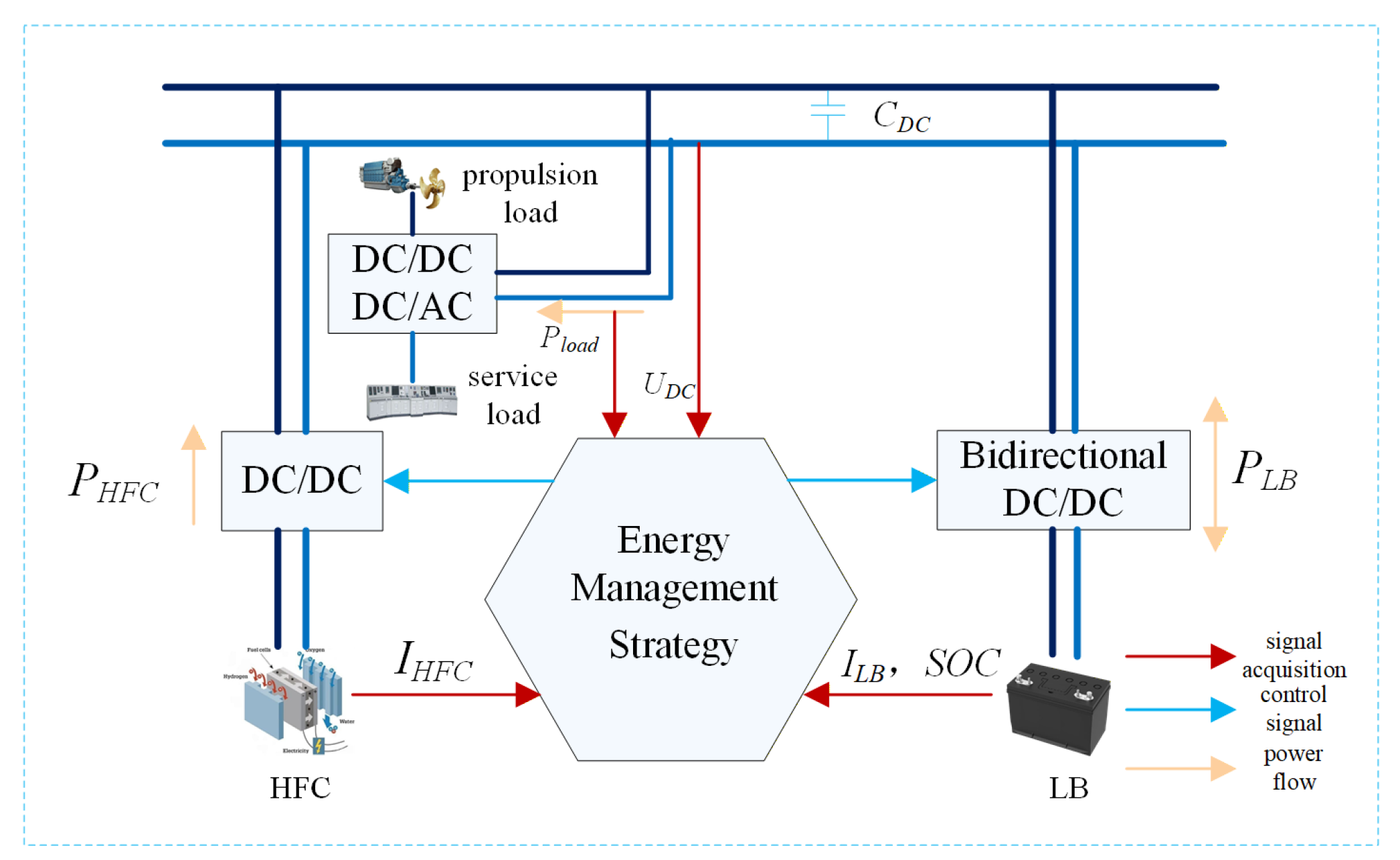
The topology structure of an HPS is shown in Figure 1, and its hybrid power system is mainly powered by multi-stack hydrogen fuel cells (HFCs), with lithium batteries (LBs) as auxiliary energy storage units. In this power system, the HFC is connected to the DC bus through a unidirectional DC/DC converter, while the LB is connected to the DC bus through a bidirectional DC/DC converter. The main load types of ships include high-power propulsion loads and service loads that maintain the basic operation of the ship. The collaborative operation and optimization control of the entire system are achieved through the EMS, which issues control instructions to each converter to allocate and schedule HFCs and LBs reasonably, thereby achieving real-time power balance between the power source and the load.

2.2. HFC Model

2.2.1. HFC Energy Costs

The HFC converts chemical energy into electrical energy through an electrochemical reaction between hydrogen and oxygen [26], and its instantaneous hydrogen consumption rate ṁ_H can be expressed as follows:

$${\dot{m}}_H={\displaystyle \frac{P_{HFC}}{{\eta }_{HFC}\cdot LH{V}_H}}$$

(1)

where η_HFC is the efficiency of the HFC, LHV_H is the lower heating value of hydrogen, and P_HFC is the output power of the HFC.

The operating cost of the HFC can be expressed as follows:

$$F_{HFC}=Q_H{\dot{m}}_H\mathrm{\Delta }t$$

(2)

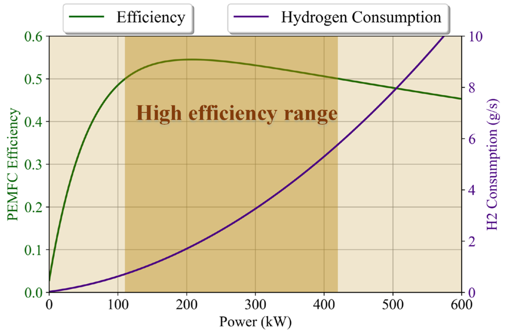
where Q_H is the selling price of hydrogen, m_H is the mass of hydrogen, and Figure 2 shows the fitted curve of efficiency versus hydrogen consumption rate.

2.2.2. HFC Battery Performance Degradation Cost

The actual operating conditions of the HFC are complex and can be roughly divided into the following categories: idle, ideal operating conditions, high power output, transient power changes, and start–stop [27], among which idle, high power, power changes, and start–stop are the main causes of HFC attenuation [28].

When the total output power of the HFC system is no higher than 20% of the maximum power, the system is considered to be in idle mode. When the total output power is no lower than 80% of the rated power, the system is considered to be in high-power output mode. The degradation costs F_HFC.l and F_HFC.h caused by idle mode and high-power output can be calculated using the following formula:

$$\begin{array}{l}{F}_{HFC.l}={\displaystyle \frac{{\alpha }_{low}{T}_{low}{Q}_{HFC}}{\mathrm{\Delta }{U}_{HFC}}}\\ F_{HFC.h}={\displaystyle \frac{{\alpha }_{high}{T}_{high}{Q}_{HFC}}{\mathrm{\Delta }{U}_{HFC}}}\end{array}$$

(3)

where α_low and α_high are the degradation rates (μV/h) of the single HFC under idle operation and high-power output conditions, respectively; T_low and T_high are the cumulative times under idle conditions and high-power operation, respectively; Q_HFC is the total price of the HFC; and ΔU_HFC represents the allowable voltage drop limit of the single HFC from the beginning of its service life to the end of its service life.

The degradation cost F_HFC.s caused by start–stop can be calculated using the following formula:

$$F_{HFC.s}={\displaystyle \frac{{\alpha }_{start}{N}_{on-off}{Q}_{HFC}}{\mathrm{\Delta }{U}_{HFC}}}$$

(4)

where α_start is the degradation rate (μV/cycle) of the monomer HFC caused by start–stop cycles; N_on-off is the number of start–stop cycles.

The degradation cost F_HFC.c caused by power changes in the HFC system can be calculated using the following formula:

$$F_{HFC.c}={\displaystyle \sum _0^t\frac{{\alpha }_{power}}{\mathrm{\Delta }{U}_{HFC}\cdot N_{HFC}}\cdot \mathrm{\Delta }{P}_{HFC}(t)\cdot Q_{HFC}}$$

(5)

where α_power is the degradation rate (μV/kW) caused by HFC power changes in the entire stack; N_HFC is the number of individual HFCs.

2.3. LB Model

2.3.1. LB Energy Cost

The LB can be represented by an equivalent internal resistance model [29], in which the output power is calculated as follows:

$$P_{LB}=U_{oc}{I}_{LB}-I_{LB}^2{R}_{in}$$

(6)

where U_oc, I_LB, and R_in represent the open-circuit voltage, battery current, and equivalent internal resistance of the lithium battery pack, respectively. During discharge, I_LB is positive.

This allows us to calculate the battery current of the battery pack I_LB:

$$I_{LB}={\displaystyle \frac{U_{\mathrm{oc}}-\sqrt{U_{\mathrm{oc}}^2-4R_{in}{P}_{LB}}}{2R_{in}}}$$

(7)

The battery current and state of charge (SOC) [30] of a single lithium battery are calculated as follows:

$$SOC=SO{C}_0-{\displaystyle \frac{1}{C_{LB}}}{\displaystyle {\int }_0^t{I}_{LB}}dt$$

(8)

where SOC₀ represents the SOC value in the initial state; C_LB represents the rated capacity of a single cell.

The electrical energy consumed by the battery can be expressed using equivalent hydrogen consumption m_LB.eq:

$$\mathrm{\Delta }SOC=-{\displaystyle \frac{I_{LB}}{3600\cdot C_{LBA}}}·\mathrm{\Delta }t$$

(9)

$$m_{LB.eq}=\left\{\begin{array}{c}{P}_{LB}·{\displaystyle \frac{1}{{\eta }_{ch.avg}·{\eta }_{dis}}}·{\displaystyle \frac{m_{HFC.avg}}{P_{HFC.avg}}},\mathrm{\Delta }SOC<0\\ P_{LB}·{\eta }_{ch}·{\eta }_{dis.avg}·{\displaystyle \frac{m_{HFC.avg}}{P_{HFC.avg}}},\mathrm{\Delta }SOC\ge 0\end{array}\right.$$

(10)

where P_LB represents the power of the battery pack; m_HFC.avg represents the average hydrogen consumption of HFC; P_HFC.avg represents the average power of HFC; η_ch and η_dis represent the charging efficiency and discharging efficiency of the battery pack, respectively; η_ch.avg and η_dis.avg represent the average charging efficiency and average discharging efficiency of the battery pack, respectively.

Therefore, the equivalent energy cost FLB of lithium batteries is

$$F_{LB}=Q_H{m}_{LB.eq}$$

(11)

where m_LB.eq represents the equivalent hydrogen consumption mass.

2.3.2. LB Performance Degradation Cost

The performance degradation of lithium-ion battery packs is influenced by various factors such as charge–discharge cycles and operating temperature [31]. Their lifespan models are highly complex and computationally demanding, so semi-empirical aging models [32] are typically used to quantify their degradation:

$$C_{\mathrm{loss}}=B\left(c\right)\cdot \exp \left({\displaystyle \frac{-E_a\left(c\right)}{RT}}\right){\left(A_h\left(c\right)\right)}^z$$

(12)

$$E_a\left(c\right)=\mathrm{31,700}-370.3c$$

(13)

where C_loss represents the percentage of battery capacity degradation; B represents the pre-exponential coefficient; c represents the battery current rate; E_a represents the activation energy; R is the molar gas constant; T is the operating temperature of the lithium battery pack; A_h(c) represents the cumulative charge–discharge ampere-hour count; z is set to 0.55.

Therefore, A_h(c) [33] can be calculated as follows:

$$A_h(\mathfrak{c})={\left({\displaystyle \frac{C_{loss}}{B(c)\cdot \exp \left(\frac{-E_a(c)}{RT}\right)}}\right)}^{1/z}$$

(14)

When the battery reaches the end of its life, the number of charge–discharge cycles K can be expressed as follows:

$$K={\displaystyle \frac{A_h(c)}{C_{LBA}}}$$

(15)

The performance degradation cost F_LB.d can be calculated as follows:

$$\begin{array}{l}SOH(k)=SOH(k-1)-{\displaystyle \frac{|I_{LB}(k-1)|t_{on}}{2K{C}_{LBA}}}\\ \hspace{1em}\hspace{1em}\hspace{1em}\hspace{0.33em}\hspace{0.33em}=SOH(k-1)-{\displaystyle \frac{|I_{LB}(k-1)|t_{on}}{2A_h(c)}}\end{array}$$

(16)

$$F_{LB.d}=\lambda Q_{LB}[SOH(k-1)-SOH(k)]$$

(17)

where SOH represents the health of lithium batteries; t_on represents operating time; λ represents the balance coefficient; and Q_LB represents the price of lithium battery packs.

2.4. Constraint Modeling

During the operation of the hybrid power system, in order to ensure the normal operation of the system, it is necessary to constrain the relevant parameters of the HFC and LB. The constraint conditions are as follows:

$$\left\{\begin{array}{c}{P}_{HFC.min}\le P_{HFC}\le P_{HFC.max}\\ P_{LB.min}\le P_{LB}\le P_{LB.max}\\ \left|\mathrm{\Delta }{P}_{HFC}\right|\le \mathrm{\Delta }{P}_{HFC.max}\\ \left|\mathrm{\Delta }{P}_{LB}\right|\le \mathrm{\Delta }{P}_{LB.max}\\ SO{C}_{min}\le SOC\le SO{C}_{max}\\ SO{H}_{min}\le SOH\end{array}\right.$$

(18)

where P_HFC and P_LB are the power of HFC and LB, respectively; ΔP_HFC and ΔP_LB are the changes in HFC power and LB power, respectively.

Table 1. HPS basic parameter information and modeling information.

Parameter	Value	Unit
Length/Width/Height	49.9/10.4/3.2	m
Maximum Speed	28	m/h
Cruising Speed	20	m/h
Rated Power of Propulsion Motor	500	W
Rated Capacity of Battery	1806	Wh
Rated Power of HFC System	500	kW
Rated DC bus voltage	650	V
Rated Voltage of Battery	537.6	V
Output Voltage of HFC System	220–380	V
αlow	8.662	μV/h
αhigh	10.00	μV/h
αstart	13.79	μV/cycle
αpower	0.04185	μV/kW
z	0.55	-
λ	15.18	-
R	8.314	J·mol−1·K−1
SOC0	60%	-
SOCmin	30%	-
SOCmax	80%	-
SOCref	50%	-
ΔPHFC.max	20	kW
ΔPLB.max	300	kW
PHFC.min/PHFC.max	50/450	kW
PLB.min/PLB.max	0/600	kW

shows the basic parameter information for modeling.

3. DEM-MPC Detailed Process

First, based on the DEM method, PLF is achieved through DCE and NNP, and PLF evaluation indicators are provided. Subsequently, a two-stage MPC framework is constructed, including the MPC basic model and hierarchical optimization modeling. Finally, DEM and MPC are integrated to form a complete DEM-MPC control process to achieve system optimization and operation.

3.1. PLF Based on DEM

3.1.1. Delay Coordinate Embedding (DCE)

For the PLF of the HPS power system, the delayed coordinate embedding method is used for state space reconstruction [34]. This method uses time delay reconstruction technology to map the one-dimensional load time series x(t) into a high-dimensional state vector to fully extract the dynamic characteristics of the system.

$$X(t)=[x(t),x(t-\tau ),x(t-2\tau ),\dots ,x(t-(E-1)\tau )]$$

(19)

where X(t) is the reconstructed E-dimensional state vector; τ is the optimal time delay; E is the embedding dimension.

Determination of time delay τ: A strategy combining the autocorrelation function method and mutual information method is adopted. First, the autocorrelation function of the load sequence is calculated, and the first zero crossing point is selected as the initial τ value. Subsequently, verification is performed based on mutual information theory, and the first minimum point of the mutual information function is selected as the optimal τ.

Autocorrelation function calculation formula:

$$R_{xx}(\tau )={\displaystyle \frac{\mathbb{E}[(x(t)-\mu )(x(t+\tau )-\mu )]}{{\sigma }^2}}$$

(20)

where μ is the mean of the time series, and σ is the standard deviation. The optimal time delay τ is taken as the first value that satisfies R_xx(τ) ≤ 1/e.

Mutual information calculation formula:

$$I(\tau )={\displaystyle \sum _{i,j}p}(x(t_i),x(t_j+\tau ))\log \left({\displaystyle \frac{p(x(t_i),x(t_j+\tau ))}{p(x(t_i))p(x(t_j+\tau ))}}\right)$$

(21)

where the optimal delay corresponds to the first minimum point of the mutual information function.

The embedding dimension E is determined by applying the false nearest neighbor point method [35], gradually increasing the E value, calculating the false neighbor point ratio, and determining the optimal E value when the ratio is less than 5%. This method can effectively avoid information loss caused by insufficient dimensions or excessive computational complexity caused by dimensional redundancy.

$$r(E)={\displaystyle \frac{\Vert X_{E+1}(t)-X_{E+1}^{(nn)}(t)\Vert }{\Vert X_E(t)-X_E^{(nn)}(t)\Vert }}$$

(22)

where X_E(t) represents the E-dimensional embedding vector, and the superscript (nn) represents the nearest neighbor point. The optimal embedding dimension E^∗ satisfies the following:

$$P(r(E^{\ast })>r_{tol})<5\%$$

(23)

3.1.2. Nearest Neighbor Prediction (NNP)

In the reconstructed state space, NNP [36] is used for prediction. The steps are as follows:

Given the current state X(t), we find its k nearest neighbors in the historical data:

$$X_{NN}^{(i)}=\arg {\min }_{X(t^{\prime })}\Vert X(t)-X(t^{\prime })\Vert ,\hspace{1em}i=1,2,\dots ,k$$

(24)

where ||·||, we use the Mahalanobis distance:

$$D(X_i,X_j)=\sqrt{{(X_i-X_j)}^T{\Sigma }^{-1}(X_i-X_j)}$$

(25)

Then, based on the selected k neighboring points, we construct a time-varying weighted prediction function:

$$\widehat{x}(t+T)={\displaystyle \sum _{i=1}^k{w}_i}(T)\cdot x(t_i+T)+ϵ(T)$$

(26)

The weighting coefficient uses a double weighting strategy, distance weighting:

$$w_i^d=\exp (-\gamma D(X(t),X_{NN}^{(i)}))$$

(27)

Time-weighted:

$$w_i^t=\exp (-\beta |t-t_i|)$$

(28)

Final weighting:

$$w_i(T)={\displaystyle \frac{w_i^d\cdot w_i^t}{{\displaystyle \sum _{j=1}^k{w}_j^d}\cdot w_j^t}}$$

(29)

Finally, we establish a probability prediction interval (PI):

$$[{\widehat{x}}_{lower},{\widehat{x}}_{upper}]=\widehat{x}(t+T)\pm z_{\alpha /2}\cdot \sigma (T)$$

(30)

$$\sigma (T)=\sqrt{{\displaystyle \frac{1}{k-1}}{\displaystyle \sum _{i=1}^k}{[x(t_i+T)-\overline{x}(T)]}^2}$$

(31)

where $\overline{x}$(T) is the mean of the nearest point prediction, and z_α/2 is the standard normal quantile.

3.1.3. PLF Evaluating Indicator

Three probability evaluation indicators are used to assess the performance of the HPS power system PLF model. The predicted interval coverage probability (PICP) is used to evaluate the statistical probability of actual observed values falling within the predicted interval range, reflecting the reliability level of the model. The prediction interval normalized average width (PINAW) objectively measures the accuracy of the prediction results by calculating the ratio of the predicted interval width to the data range.

$$PICP={\displaystyle \frac{1}{N}}{\displaystyle \sum _{i=1}^N{b}_i},b_i=\left\{\begin{array}{c}1,\begin{array}{cc}& y_i\in \left[P_{Li},P_{Ui}\right]\end{array}\\ 0,\begin{array}{cc}& y_i\notin \left[P_{Li},P_{Ui}\right]\end{array}\end{array}\right.$$

(32)

$$PINAW={\displaystyle \frac{1}{N}}{\displaystyle \sum _{i=1}^N\frac{\left(P_{Ui}-P_{Li}\right)}{y_{\max }-y_{\min }}}$$

(33)

where N is the total number of samples, P_Ui and P_Li represent the prediction interval range at the i-th time point. We define the indicator function b_i∈{0,1}, such that bi = b_i when the actual value y_i∈[P_Li, P_Ui], and 0 otherwise. We let y_max and y_min denote the maximum and minimum values of the target parameter over the entire prediction time domain, respectively.

Under the given confidence level requirements, a high-quality prediction interval must simultaneously satisfy two key characteristics: the interval width should be as compact as possible while ensuring sufficient coverage probability. The PINAW of the prediction interval should be small, reflecting the precision of the prediction results; while the PICP should be maintained at a high level, reflecting the reliability of the prediction results. To comprehensively evaluate these two important metrics, this study adopted the coverage-width criterion (CWC) as a composite evaluation standard for a comprehensive assessment of prediction performance.

$$\left\{\begin{array}{l}CWC=PINAW\left(1+\gamma e^{-\beta \left(PICP-\alpha \right)}\right)\\ \gamma =\left\{\begin{array}{c}0,\begin{array}{cc}& PICP\ge \alpha \end{array}\\ 1,\begin{array}{cc}& PICP<\alpha \end{array}\end{array}\right.\end{array}\right.$$

(34)

where β is used as the penalty coefficient for PICP that does not meet the standard, and α represents the nominal confidence level that PICP must meet.

3.2. Two-Stage MPC Modeling and Optimization

Based on the multi-step PLF provided by DEM, the two-stage MPC developed in the first step optimizes the efficiency of the HFC system and maintains the SOC status of the LB. The second step optimizes the overall cost of the hybrid system, including energy consumption and equipment degradation.

3.2.1. MPC

MPC calculates the future historical state of N_p steps based on historical information and future inputs to the system [37], expressed as follows:

$$\begin{array}{l}x(k+1)=Ax(k)+Bu(k)\\ x(k+2)=A^{2}x(k)+ABu(k)+Bu(k+1)\\ \cdot \cdot \cdot \cdot \cdot \cdot \cdot \cdot \\ x(k+N_p)=A^{N_p}x(k)+A^{N_p-1}Bx(k)+\cdot \cdot \cdot \cdot +Bu(k+N_p)\end{array}$$

(35)

where A and B are coefficient matrices; x(k) and u(k) are state variables and control variables, respectively. This paper controls four independent fuel cell stacks and batteries in the HFC system and maintains the SOC within the reference range. The single-step state and control variables are the following:

$$x(k)=[{\dot{m}}_{H\_HFC1}:{\dot{m}}_{H\_HFC2}:{\dot{m}}_{H\_HFC3}:{\dot{m}}_{H\_HFC4}:SOC{]}_k^{\mathrm{T}}$$

(36)

$$u(k)={\left[P_{FC1}^{ref}:P_{FC2}^{ref}:P_{FC3}^{ref}:P_{FC4}^{ref}:P_{LB}\right]}_k^{\mathrm{T}}$$

(37)

3.2.2. Two-Stage Optimization Modeling

In the first optimization step, the efficiency of the HFC system for the next N_p moments is optimized to get as close as possible to the maximum efficiency point. At the same time, the deviation range between SOC and the reference value needs to be ensured. The cost function is given in Formula (37), and Formula (38) calculates the efficiency of the HFC system based on four independent fuel cell stacks.

$$J_1:\min {\displaystyle \sum _{n=1}^{Np}[{\lambda }_1\cdot {(\frac{\eta (k+n)-{\eta }_{max}}{{\eta }_{max}})}^2}+{\lambda }_2\cdot {(SOC(k+n)-SO{C}_{ref})}^2$$

(38)

$$\eta ={\displaystyle \frac{{\displaystyle \sum _{i=1}^{I=4}{P}_{HFCi}}}{{\displaystyle \sum _{i=1}^{I=4}\frac{P_{HFCi}}{{\eta }_{HPCi}}}}}$$

(39)

where λ₁ and λ₂ are optimization weights. Due to fluctuations in load demand, pursuing the maximum efficiency point of the HFC will cause fluctuations in the SOC, and the weights need to be set according to the tendency.

The optimization results u(k + 1), …, u(k + N_p) obtained in the first step of MPC are applied to the system model. Subsequently, the output [$P_{FC1}^{ref}$ : $P_{FC2}^{ref}$ : $P_{FC3}^{ref}$ : $P_{FC4}^{ref}$] of the HFC system over N_p steps is used as the reference power sequence for the hydrogen fuel cell, and the second step of MPC optimization is performed.

In the second optimization step, the objective is to minimize the total cost, and the constraints in the optimization model are the same as those in Equation (17). The control variable optimized in the first step, u*(k + 1), is used as the final control output. The cost optimization function is as follows:

$$J_2:\min {\displaystyle \sum _{n=1}^{Np}[C_{FC\_total}}(k+n)+C_{bat\_total}(k+n)+Q_{PC}(k+n)]$$

(40)

$$Q_{PC}(k+n)=\alpha \cdot {\displaystyle \sum _{i=1}^{I=4}\left|P_{FCi}\right.}(k+n)-P_{FCi}^{ref}(\left.k+n)\right|$$

(41)

where Q_PC is used as a penalty term, and α is the penalty coefficient, which limits the deviation between the final HFC system output and the reference power, thereby maximizing energy efficiency.

3.3. DEM-MPC Process

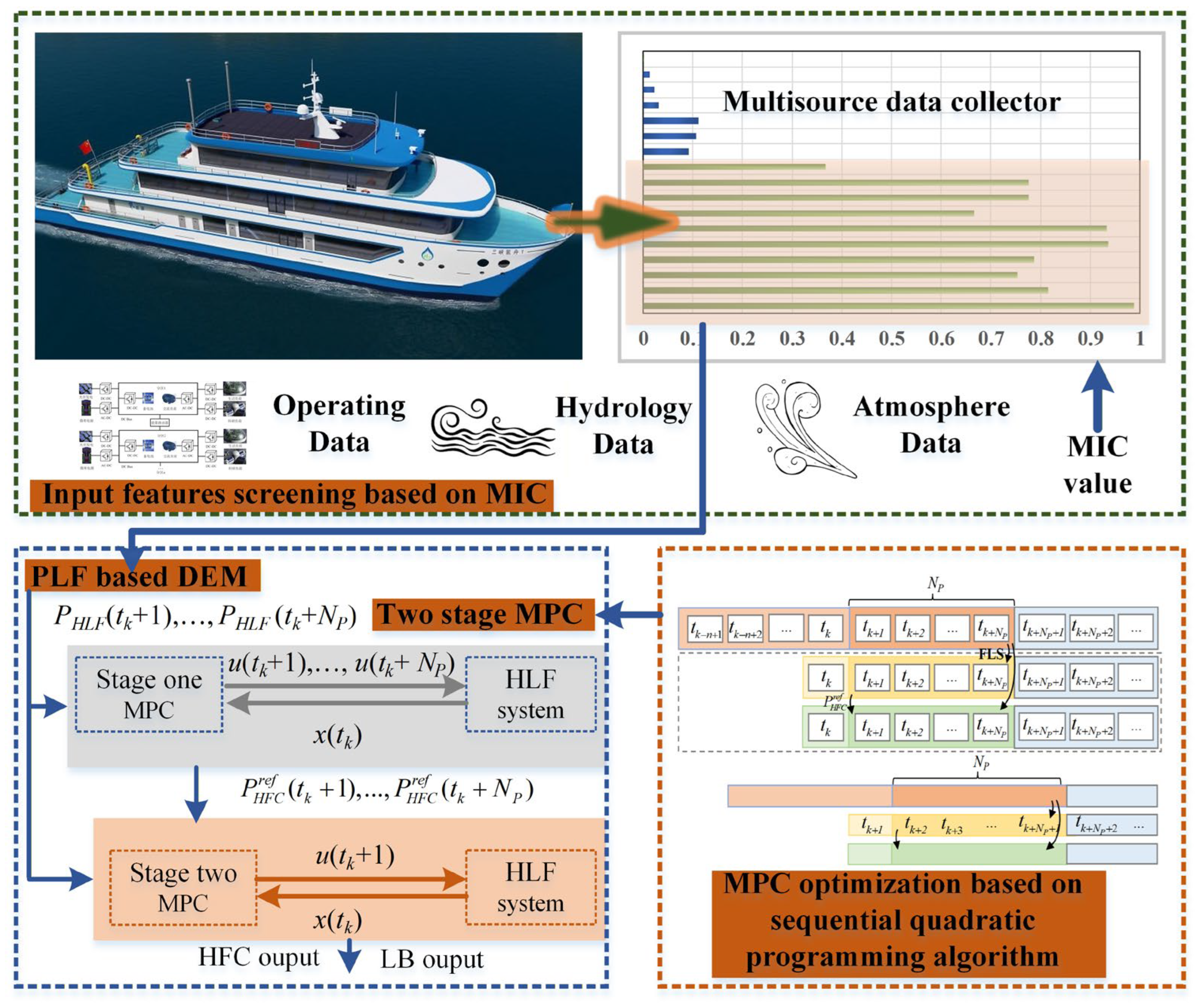
The workflow of the DEM-MPC framework (Figure 3) primarily consists of three key stages:

(1)

Multi-source data collection and processing. The system collects three types of core data in real time: channel hydrological parameters (including changes in flow velocity and water depth), environmental meteorological information (such as wind speed and temperature), and the operational status of the vessel’s propulsion system (including working parameters of fuel cells and lithium batteries). Through maximum information coefficient (MIC) analysis [38], the key parameters most influential to load prediction are identified.

(2)

DEM dynamic load prediction modeling. The DEM model integrates channel water depth, flow velocity, and other hydrological features, as well as wind speed, temperature, and other meteorological parameters, to accurately capture the dynamic impact of environmental factors on vessel load. This data-driven approach does not require the prior establishment of precise physical models but, instead, directly learns the system’s dynamic characteristics from historical data, making it particularly suitable for addressing load prediction issues for hydrogen-powered vessels in complex channel conditions.

(3)

Two-stage MPC optimization. The first-stage optimization focuses on equipment efficiency to determine the baseline power output of the fuel cell; the second-stage optimization comprehensively considers operational economics and equipment protection factors, generating final control commands through an iterative optimization algorithm. The entire optimization process is executed in a fixed-cycle rolling manner, dynamically adjusting the power allocation ratio between the fuel cell and lithium-ion battery to ensure the system remains in an optimal operational state at all times.

Figure 3. DEM-MPC detailed flowchart.

Figure 3. DEM-MPC detailed flowchart.

4. Case Study

This study uses actual ship operation data from the “Three Gorges Hydrogen Boat No. 1” to experimentally validate the proposed method. Based on DEM, a PLF interval prediction sequence is generated and compared with the prediction results of multiple benchmark models. Subsequently, the proposed two-stage MPC is comprehensively compared with three typical energy management strategies: rule-based control, single-stage MPC, and dynamic programming. Table 1 shows the main parameters of the HPS.

4.1. PLF Test Results

4.1.1. Dataset Introduction and Variable Selection

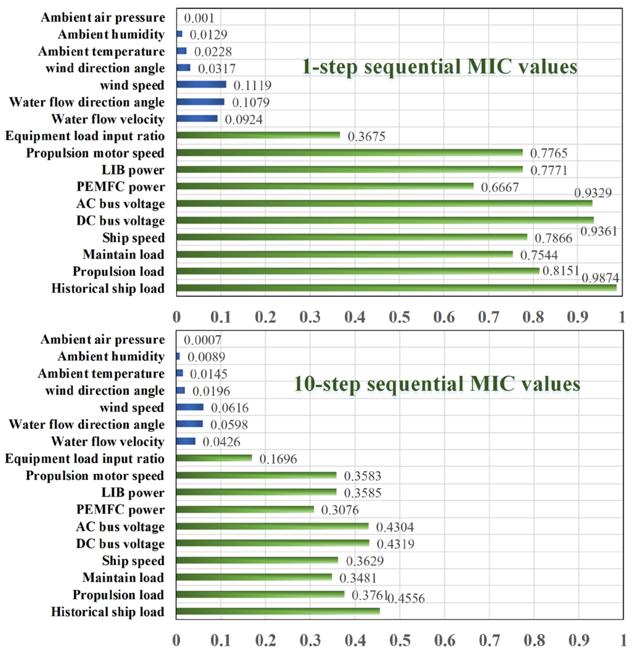
Based on the navigation data from the “Three Gorges Hydrogen Boat No. 1” in October 2023 (sampling frequency of 1 Hz, totaling 252,000 data points), the system collected multi-dimensional features including power system status parameters, navigation conditions, and environmental monitoring data. Through MIC analysis (as shown in Figure 4), the nonlinear correlation between each feature and the load prediction values for the next 10 time steps was evaluated. Ultimately, 10 key features marked with green bars in Figure 4 were selected as inputs for the prediction model. These green-labeled indicators all possess significantly higher maximum information coefficient values compared with environmental parameters such as air pressure and wind direction angle, which display negligible correlation with ship load. MIC quantifies the nonlinear coupling strength between each variable and future power demand; only the 10 features with prominent MIC scores can effectively reflect load dynamic evolution. Excluding low-correlation environmental variables reduces model-redundant input dimensions and cuts computational overhead, while retaining core physical factors that dominate short-term and long-term load fluctuations.

Consistent with the 1 Hz sampling frequency of ship navigation monitoring data, the energy management controller operates under the identical 1 Hz sampling cycle, meaning the 10-step prediction window precisely corresponds to a 10 s forward rolling horizon, which conforms to the reviewer’s deduction. This 10 s prediction span is deliberately designed to strike a balance between optimization performance and on-board real-time computing capacity. In theory, extending the prediction length may bring marginal additional optimization benefits, while contrast experiments with the global optimization strategy confirm that the 10 s window can capture nearly all major efficiency and economic gains available. Longer prediction horizons would introduce massive extra computation burden and cause control delay that fails to meet the real-time demand of ship power systems. Therefore, the 10-step prediction length is a practical trade-off, which can realize most optimization potential without sacrificing the real-time response capability required for vessel energy management.

4.1.2. Prediction Results and Analysis

To validate the superiority of the DEM model, comparative experiments were conducted using ARIMA [39], support vector regression (SVR) [40], and neural networks (NNs) [41]. All models utilized the same input features and dataset, with a prediction step size of 10.

The comparative analysis in

Table 2. Statistics of multiple prediction model indicators.

Horizon	Model	Indicator Statistics
		PICP	PINAW	CWC	Forecast Time (s)
1-step	ARIMA	0.9313	0.1984	0.5461	0.0297
	SVR	0.9370	0.1863	0.4615	0.0779
	NN	0.9447	0.1841	0.3999	0.1756
	DEM	0.9501	0.1754	0.1754	0.0363
3-step	ARIMA	0.9126	0.2247	0.9148	0.0326
	SVR	0.9183	0.2111	0.7575	0.0857
	NN	0.9257	0.2086	0.6410	0.1932
	DEM	0.9311	0.1987	0.5490	0.0399
5-step	ARIMA	0.8853	0.2644	2.1061	0.0356
	SVR	0.8907	0.2483	1.7192	0.0934
	NN	0.8980	0.2455	1.4138	0.2107
	DEM	0.9032	0.2338	1.1857	0.0435
10-step	ARIMA	0.8498	0.2909	6.1689	0.0386
	SVR	0.8551	0.2731	4.9803	0.1012
	NN	0.8621	0.2701	4.0437	0.2283
	DEM	0.8671	0.2573	3.3514	0.0471

demonstrates that the DEM model exhibits significant advantages in ship load prediction. Within the 1–10-step prediction range, the DEM model consistently achieved the highest PICP (0.9501–0.8671) and lowest PINAW (0.1754–0.2573), with CWC values (0.5461–3.3514) outperforming the comparison models, indicating more reliable interval prediction performance. Notably, the DEM model excels in computational efficiency, with prediction times (0.0363–0.0471 s) comparable to those of lightweight ARIMA models and significantly lower than those of computationally intensive NN models (0.1756–0.2283 s). This dual advantage in prediction accuracy and computational efficiency makes the DEM model particularly suitable for real-time application requirements in ship energy management systems. As the prediction step length increases, the performance metrics of all models exhibit the expected downward trend, but the DEM model consistently maintains the best prediction stability, thanks to its dynamic empirical modeling method effectively capturing the system’s nonlinear characteristics, thereby balancing prediction accuracy and real-time requirements.

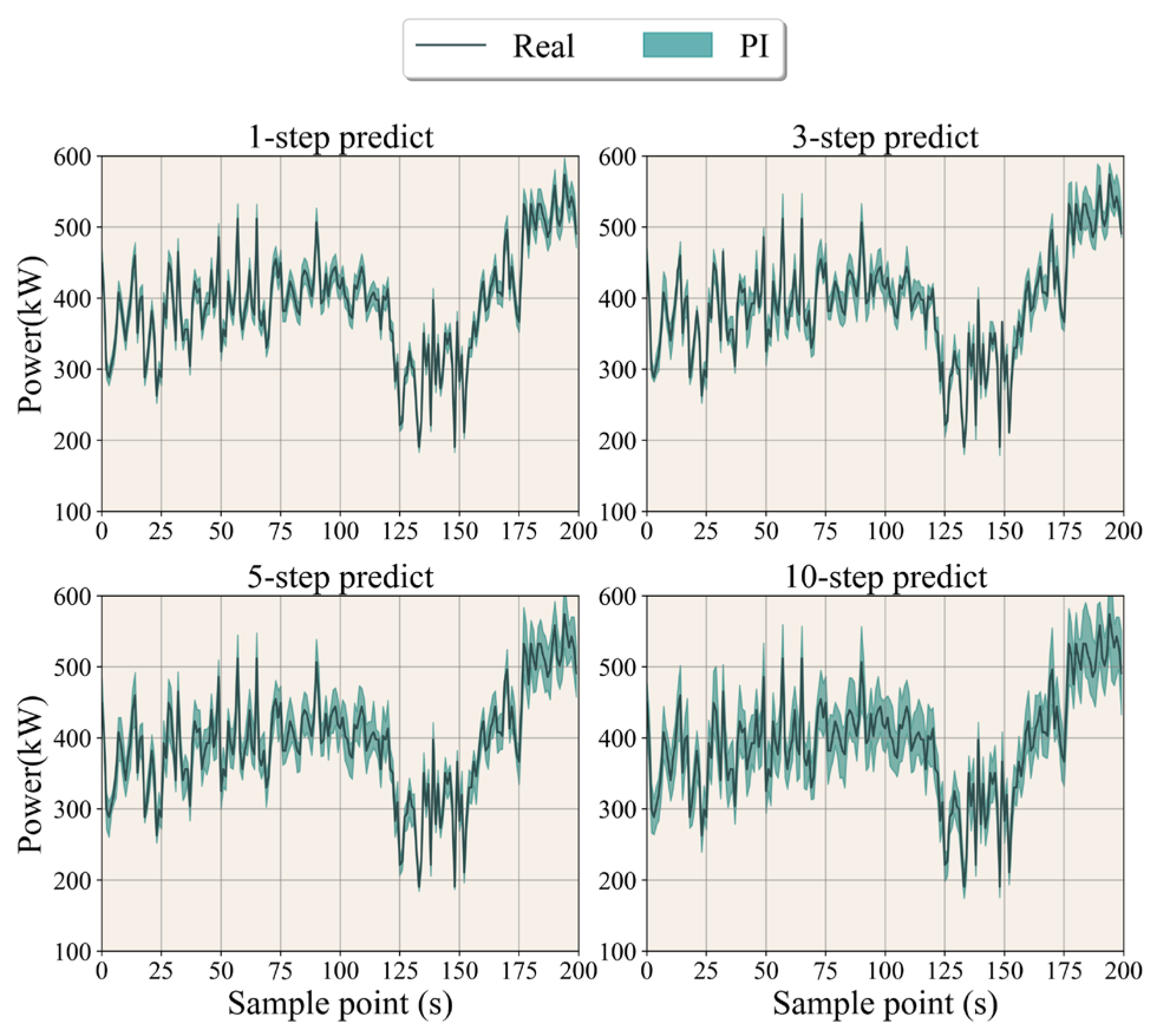
Figure 5 shows the comparison between the 1-step, 3-step, and 5-step prediction PI and the actual load. In the 1-step prediction, the prediction curve closely matches the actual power changes, demonstrating the DEM model’s precise capture of short-term load fluctuations. As the prediction step length increases to three steps and five steps, the prediction error gradually increases, but the overall trend remains consistently good, particularly at load inflection points where the direction of change is accurately predicted. This indicates that the proposed method possesses good multi-step prediction capabilities in ship energy management, providing reliable input for real-time optimization control.

4.2. Optimization of Experimental Results Analysis

To demonstrate the effectiveness of DEM-MPC, three existing EMS strategies were used for comparison: rule-based power following strategy (PFS) [42], equivalent hydrogen consumption minimization strategy (ECMS) [43], classical MPC [19], and global optimization (GO) strategy [44] as a perfect control.

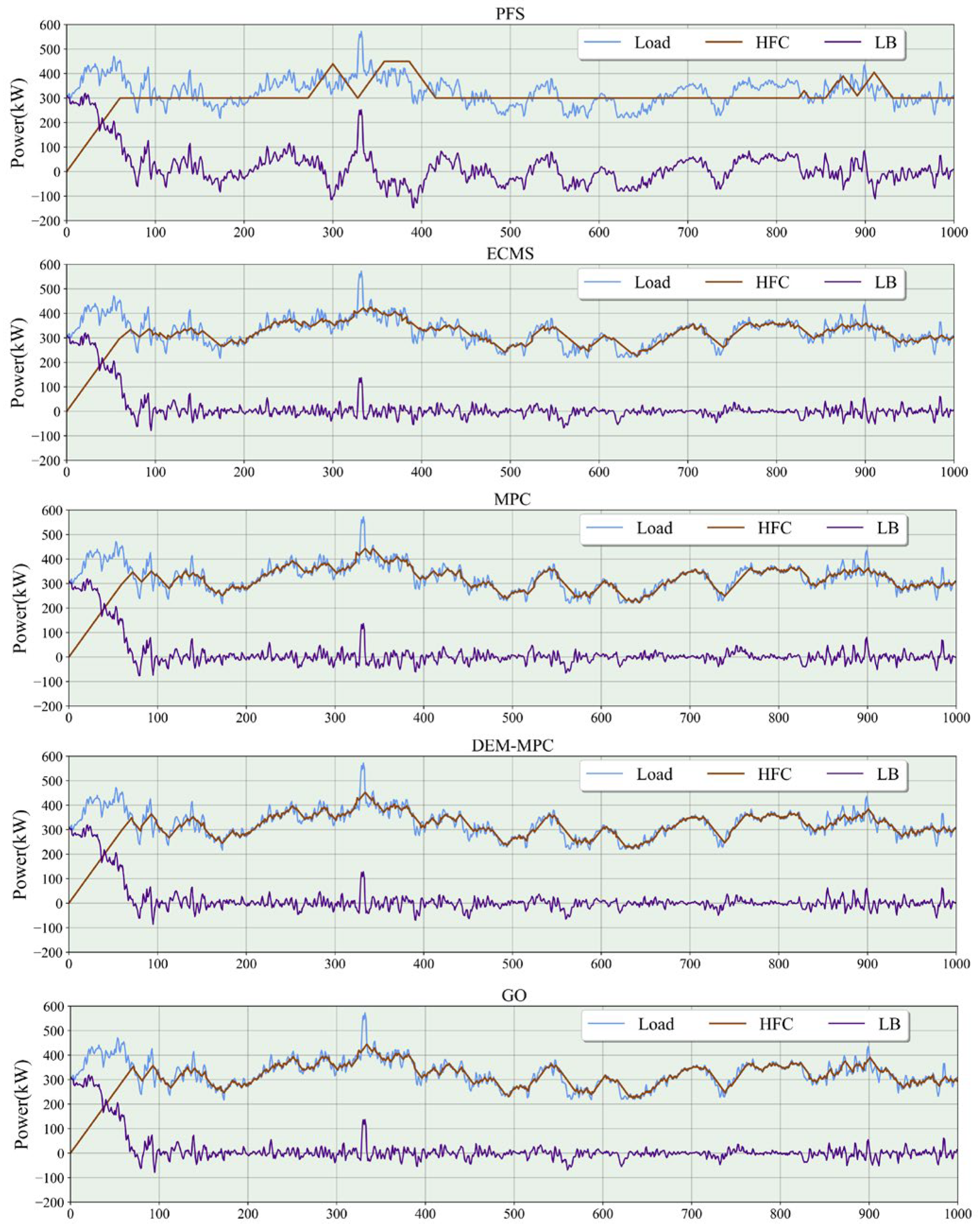
The basic principle of PFS is to ensure that the output power of the PEMFC system follows changes in the required power according to a pre-designed ratio, while maintaining the SOC within a reasonable range. PFS sets the PFC_rep reference value to 300 kW. The specific PFS design is as follows:

The remaining methods use the same constraints and parameter settings as DEM-MPC, and all use the mature nonlinear optimization algorithm of sequential quadratic programming [45] to optimize and solve the cost function, with the solution length N_P set to 10 steps.

4.2.1. HFC and LB Power Distribution

The power distribution comparison results shown in Figure 6 indicate that the DEM-MPC strategy demonstrates significant advantages in terms of dynamic response. Benefiting from the multi-step probabilistic load forecasting module embedded in the DEM framework, the method can quantitatively characterize the stochastic uncertainty of future ship power demand, and pre-compensate the power allocation reference sequence according to the prediction interval boundary of fluctuating loads. Under conditions of rapid load fluctuations, DEM-MPC can achieve a smooth transition in HFC power output, with a more gradual change in the power curve compared to the traditional PFS strategy, effectively avoiding sharp fluctuations in power output triggered by unpredictable load deviations. Additionally, this strategy coordinates power allocation between the HFC and LB, fully considering the uncertainty risk of real-time power mismatch caused by load forecasting errors, ensuring more harmonious power output coordination between the two, resulting in more stable overall system operation. Compared to the classic MPC strategy without uncertainty quantification, DEM-MPC exhibits faster response speeds during sudden load changes while maintaining better power tracking accuracy under stochastic load disturbances. DEM-MPC also closely aligns with GO in terms of power output trends. These characteristics indicate that DEM-MPC can better adapt to the dynamic, uncertain demands of ship propulsion systems, providing an optimal energy management solution for hybrid propulsion systems.

4.2.2. HFC Operating Efficiency

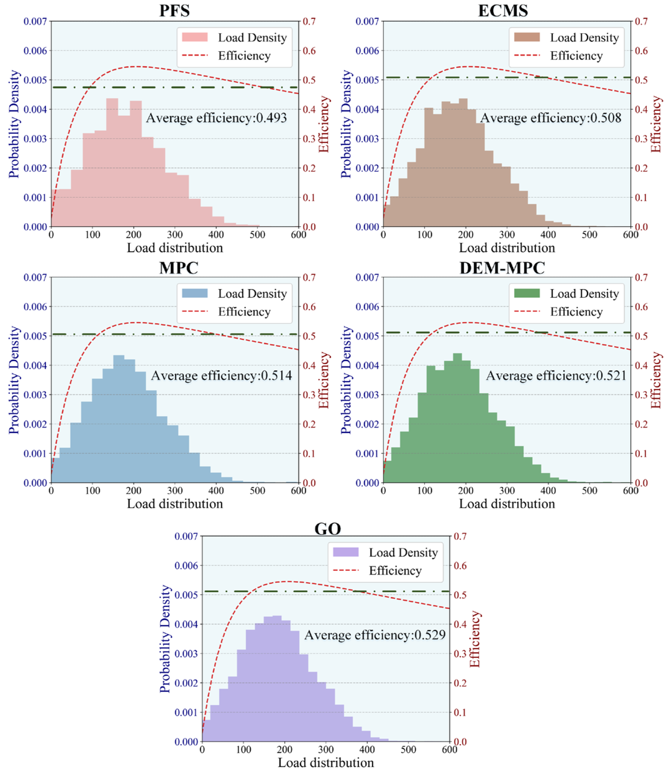
Figure 7 shows the comparison results of different energy management strategies in terms of load density efficiency. From the overall trend, the DEM-MPC strategy demonstrates a significant advantage in load allocation efficiency, with an average efficiency value between the traditional MPC strategy and the GQ strategy, showing good comprehensive performance. Specific analysis shows that the DEM-MPC strategy has the most balanced load density distribution, avoiding local inefficiencies induced by unconsidered load uncertainty. Compared with the PFS strategy that ignores load randomness, the DEM-MPC strategy significantly improves the overall system efficiency; compared with the classic MPC strategy relying on deterministic single-point prediction, although the efficiency improvement is not obvious under ideal deterministic loads, the load distribution curve is smoother under uncertain fluctuating scenarios, indicating better dynamic adaptability; compared with the ECMS strategy, the DEM-MPC strategy achieves better load balancing while maintaining a similar average efficiency. Notably, the efficiency performance of the DEM-MPC strategy is close to that of the GO strategy, indicating that this strategy can effectively approximate the theoretical optimal solution while ensuring real-time performance and robust handling of load uncertainty. This balanced performance is primarily attributed to the DEM-MPC strategy’s integration of the predictive uncertainty quantification advantages of dynamic experience modeling and the optimization capabilities of model predictive control, enabling it to allocate system load more reasonably and thereby enhance overall operational efficiency under stochastic navigation conditions.

4.2.3. Operating Costs

Table 3. Cruising and working condition cost statistics.

Operating Conditions	Method	Cost Statistics (USD)
		FHFC	FLB	FHFC.d	FLB.d	Ftotal
Cruising condition	PFS	332.8485	76.2926	7.0451	2.1130	418.2992
	ECMS	316.9985	74.5643	6.7096	2.0124	400.2849
	MPC	323.3385	59.4858	6.8438	1.9319	391.6000
	DEM-MPC	329.8053	48.4379	6.9807	1.8546	387.0785
	GO	313.2360	54.5802	6.3714	1.8997	376.0873
Working condition	PFS	182.1128	78.7734	3.8123	3.9350	268.6335
	ECMS	198.1241	46.6027	4.1935	1.2578	250.1781
	MPC	202.0866	37.1786	4.2774	1.2074	244.7500
	DEM-MPC	206.1283	30.2737	4.3629	1.1591	241.9241
	GO	195.7725	34.1126	3.9821	1.1873	235.0545

shows a comparison of the comprehensive costs of different energy management strategies under two operating conditions: cruising and operation. All cost indicators are calculated considering the uncertainty penalty term derived from the probabilistic load prediction interval, which quantifies the extra economic loss brought by load forecasting bias. Under cruising conditions, the DEM-MPC strategy performed best with a total cost of $387.08, which is 7.5% lower than the PFS strategy and 3.3% lower than the ECMS strategy. Although its HFC direct cost is slightly higher than that of the MPC strategy, it achieves better overall economic efficiency through optimized LB usage and advance response to uncertain load spikes. Notably, the DEM-MPC strategy exhibits suboptimal performance in terms of HFC degradation costs and LB degradation costs, demonstrating excellent equipment protection characteristics against random load shocks. Under working conditions with stronger load uncertainty, the DEM-MPC strategy continues to maintain its advantage, with significantly lower LB usage costs than other strategies, indicating that this strategy can effectively coordinate the usage ratio of the two energy sources under different operating conditions with distinct stochastic load features. Compared to the GO strategy, the cost differences between the DEM-MPC strategy and the GO strategy under the two operating conditions are 2.9% and 3.5%, respectively, demonstrating performance close to the theoretical optimum even after introducing uncertainty loss assessment.

Table 4. HFC single-item depreciation cost statistics.

Operating Conditions	Method	HFC Degrade Cost Statistics (USD)
		FHFC.s	FHFC.c	FHFC.h	FHFC.l
Cruising condition	PFS	0.1409	4.9316	0.3523	1.6204
	ECMS	0.1342	5.3677	0.3355	0.8723
	MPC	0.1369	5.4751	0.3422	0.8897
	DEM-MPC	0.1396	5.5846	0.3490	0.9075
	GO	0.1274	5.0971	0.3186	0.8283
Working condition	PFS	0.0762	1.9062	0.1906	0.3050
	ECMS	0.0839	3.3548	0.2097	0.5452
	MPC	0.0855	3.4219	0.2139	0.5561
	DEM-MPC	0.0873	3.4904	0.2181	0.5672
	GO	0.0796	3.1857	0.1991	0.5177

provides a detailed analysis of the impact of each strategy on HFC degradation costs, where all degradation metrics account for the uncertainty-induced frequent power switching risks. In cruise conditions, the HFC start–stop costs and power change costs of DEM-MPC are slightly higher than those of the MPC strategy but significantly better than those of the PFS strategy. This indicates that DEM-MPC effectively reduces mechanical stress on the HFC through smooth power regulation that offsets uncertain load jumps. Under working conditions with severe random load variations, although the degradation cost metrics of DEM-MPC are slightly higher than those of MPC, its power variation cost is more balanced than that of ECMS, thereby avoiding damage to the HFC caused by extreme operating conditions triggered by unpredicted load shifts. Comprehensive analysis indicates that DEM-MPC achieves the optimal balance between operational stability and economic efficiency in controlling HFC degradation with full consideration of load uncertainty, making it particularly suitable for the long-term operational requirements of ships under complex stochastic waterway environments.

4.3. Further Discussion and Analysis

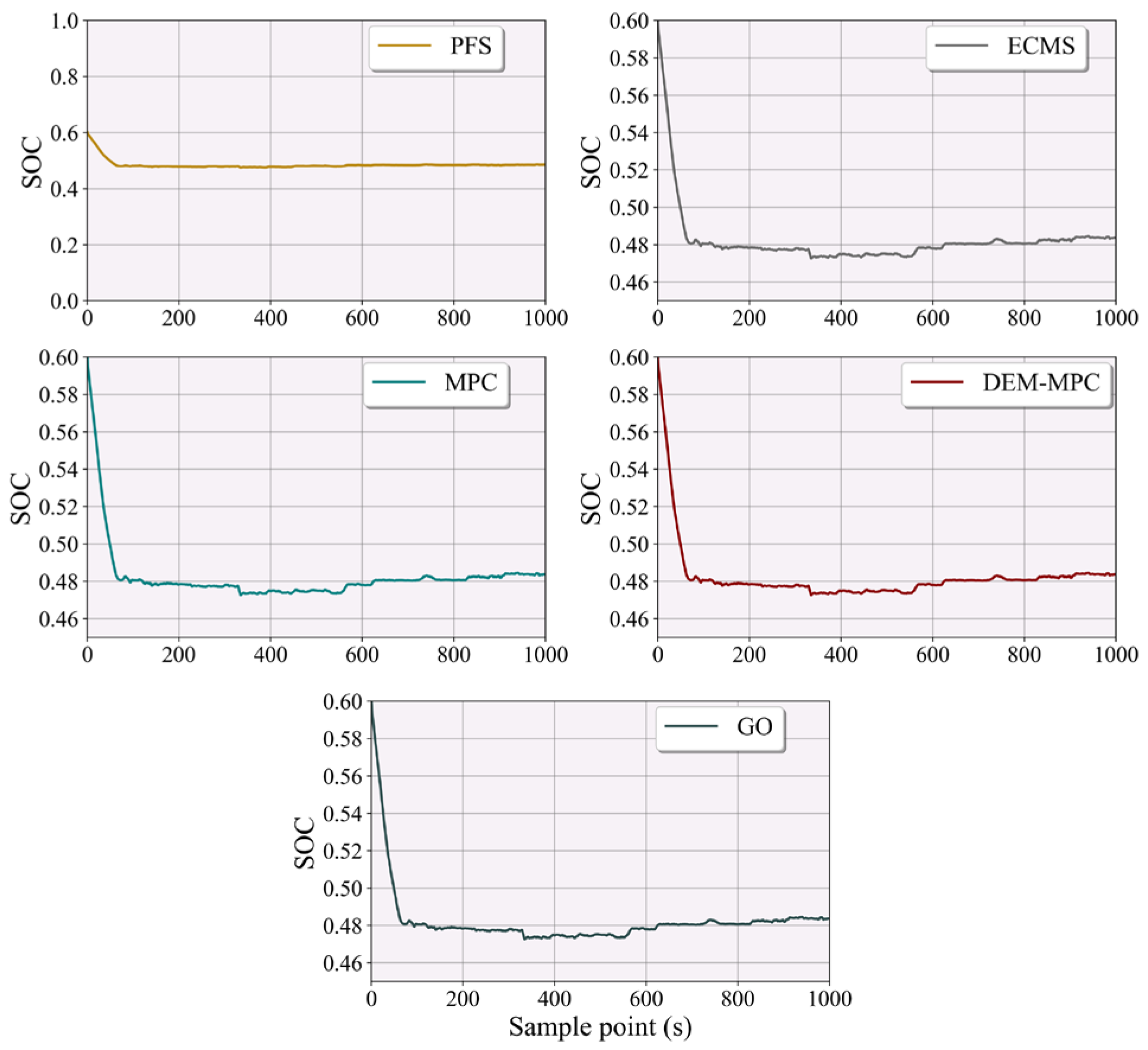
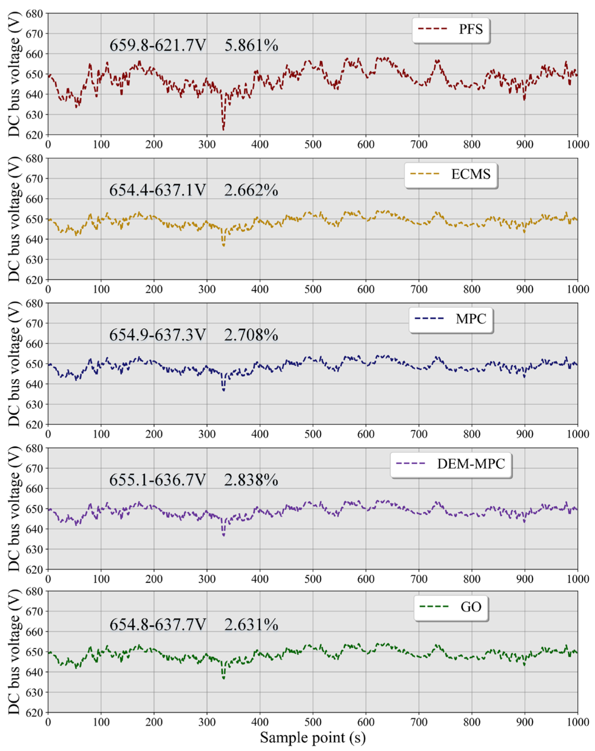
Figure 8 shows a performance comparison of different energy management strategies in terms of SOC maintenance and DC bus voltage stability. From the SOC change curve, it can be seen that the SOC fluctuation range of the DEM-MPC strategy is between 0.46 and 0.5, demonstrating better energy storage management capabilities to resist uncertain load impact compared to PFS. The voltage data in Figure 9 shows that DEM-MPC controls DC bus voltage fluctuations within a range of 2.708%, significantly outperforming ECMS’s 5.861%, indicating its stronger voltage regulation capability against random power disturbances.

Further analysis indicates that DEM-MPC’s advantages in SOC and voltage control stem from its unique predictive optimization mechanism with complete uncertainty analysis. By accurately predicting load demand and deriving the probability interval of future power variation through dynamic empirical modeling, the two-stage optimization algorithm reserves reasonable power margin to counteract prediction uncertainty, and it achieves stable maintenance of SOC and precise voltage control. Especially during the 300–400 s load surge phase with prominent load randomness, DEM-MPC can quickly adjust power allocation according to the predicted uncertainty boundary, control SOC fluctuation amplitude, and suppress voltage transient fluctuations within 3%. This coordinated control capability with embedded uncertainty compensation ensures the stable operation of the hybrid system under various operating conditions with stochastic load interference.

5. Conclusions and Future Work

This article proposes a two-stage energy management framework DEM-MPC to address the issues of high load fluctuations and difficulty in energy management for HPS in complex navigational environments. By integrating HPS operation status with channel hydrometeorological data, the DEM module utilizes DCE and NNP methods to achieve high-precision multi-step PLF, providing reliable input for MPC optimization. The two-stage optimization strategy of MPC focuses on the efficiency optimization and comprehensive cost control of HFCs and LBs, effectively solving the difficult problem of balancing economy and equipment performance in traditional single objective optimization. The verification based on actual ship data in the Yangtze River channel shows that the proposed framework significantly improves the overall energy efficiency of the system. DEM-MPC achieves performance close to the global optimum (with a difference of less than 3%) while ensuring real-time performance, providing a solution that combines theoretical innovation and practicality for the engineering application of hydrogen powered ships.

Future research can be conducted from three aspects: (1) Further integration of deep learning techniques to enhance the robustness of DEM models in predicting extreme weather conditions; (2) Consider expanding the hybrid system of multi-energy ships (such as introducing wind and solar energy) and improving the multi-objective optimization framework of MPC; (3) Develop an online EMS platform that combines digital twin technology and adaptive parameter updates to achieve full lifecycle performance optimization: these improvements will drive the development of hydrogen powered ships towards smarter and more reliable directions; (4) Carry out comparative experiments under highly fluctuated, extreme abrupt power profiles involving large load startup/shutdown and sharp speed shifts, to systematically benchmark the robustness of the DEM-MPC framework against the traditional PFS energy management strategy.

References

1. International Energy Agency (IEA). Global Hydrogen Review 2026; IEA Publications: Paris, France, 2026. [Google Scholar]
2. Nebey, A.H. Recent advancements in hydrogen production from renewable energy sources. Energy Convers. Manag. X 2026, 30, 101717. [Google Scholar] [CrossRef]
3. Dall’Armi, C.; Pivetta, D.; Taccani, R. Hybrid PEM fuel cell power plants fuelled by hydrogen for improving sustainability in shipping: State of the art and review on active projects. Energies 2023, 16, 2022. [Google Scholar] [CrossRef]
4. Xie, P.; Tan, S.; Bazmohammadi, N.; Guerrero, J.M.; Vasquez, J.C. A real-time power management strategy for hybrid electrical ships under highly fluctuated propulsion loads. IEEE Syst. J. 2023, 17, 123–135. [Google Scholar] [CrossRef]
5. Bai, M.; Ke, W.; Wu, C.; Cheng, H.; Zhang, J.; Yang, X. Energy management strategies for fuel cell hybrid ships: Classification, comparison, and outlook. Energies 2026, 19, 1171. [Google Scholar] [CrossRef]
6. Bouguerra, A.; Badoud, A.E.; Mekhilef, S.; Deghfel, N.; Hmad, J. An intelligent energy management strategy for standalone PV–fuel cell–battery system using elk herd optimization approach. Energy Convers. Manag. X 2026, 30, 101826. [Google Scholar] [CrossRef]
7. Gao, J.; Sun, F.; He, H.; Zhu, G.; Strangas, E. A comparative study of supervisory control strategies for a series hybrid electric vehicle. In Proceedings of the Asia-Pacific Power and Energy Engineering Conference, Wuhan, China, 28–30 March 2009; pp. 1–7. [Google Scholar]
8. Peng, X.; Chen, H.; Guan, C. Energy management optimization of fuel cell hybrid ship based on particle swarm optimization algorithm. Energies 2023, 16, 1373. [Google Scholar] [CrossRef]
9. Jouili, K.; Jouili, M.; Mohammad, A.; Babqi, A.J.; Belhadj, W. Neural network energy management-based nonlinear control of a DC micro-grid with integrating renewable energies. Energies 2024, 17, 3345. [Google Scholar] [CrossRef]
10. Ma, L.; Yang, P.; Gao, D.; Bao, C. A multi-objective energy efficiency optimization method of ship under different sea conditions. Ocean Eng. 2023, 290, 116337. [Google Scholar] [CrossRef]
11. Jamma, M.; Builo, P.; Ulleberg, Ø. Optimal operation of maritime hybrid fuel cell/battery power systems via a real-time energy management approach—A tugboat case study. Energy Convers. Manag. X 2026, 30, 101780. [Google Scholar] [CrossRef]
12. Fang, S.; Xu, Y.; Li, Z.; Zhao, T.; Wang, H. Two-step multi-objective management of hybrid energy storage system in all-electric ship microgrids. IEEE Trans. Veh. Technol. 2019, 68, 3361–3373. [Google Scholar] [CrossRef]
13. Wang, X.; Zhu, H.; Luo, X.; Chang, S.; Guan, X. A novel optimal dispatch strategy for hybrid energy ship power system based on the improved NSGA-II algorithm. Electr. Power Syst. Res. 2024, 232, 110385. [Google Scholar] [CrossRef]
14. Rafiei, M.; Boudjadar, J.; Khooban, M.H. Energy management of a zero-emission ferry boat with a fuel-cell-based hybrid energy system: Feasibility assessment. IEEE Trans. Ind. Electron. 2021, 68, 1354–1363. [Google Scholar] [CrossRef]
15. Si, Y.P.; Wang, R.J.; Zhang, S.Q.; Zhou, W.; Lin, A.; Zeng, G. Configuration optimization and energy management of hybrid energy system for marine using quantum computing. Energy 2022, 253, 124131. [Google Scholar] [CrossRef]
16. Li, Z.; Wang, K.; Hua, Y.; Liu, X.; Ma, R.; Wang, Z.; Huang, L. GA-LSTM and NSGA-III-based collaborative optimization of ship energy efficiency for low-carbon shipping. Ocean Eng. 2024, 312, 119190. [Google Scholar] [CrossRef]
17. Jiang, J.; Zou, L.; Zhang, L.; Wang, H.; Wang, Y.; Liu, X. A three-layer energy management system for hydrogen-powered ships combined instantaneous load forecasting. Electr. Power Syst. Res. 2025, 243, 111494. [Google Scholar] [CrossRef]
18. Fathy, A.; Rezk, H.; Nassef, A.M. Robust hydrogen-consumption-minimization strategy based salt swarm algorithm for energy management of fuel cell/supercapacitor/batteries in highly fluctuated load condition. Renew. Energy 2019, 139, 147–160. [Google Scholar] [CrossRef]
19. Mahmood, F.; Govindan, R.; Al-Ansari, T. Efficient energy management and temperature control of a high-tech greenhouse using an improved data-driven model predictive control. Energy Convers. Manag. X 2025, 26, 100939. [Google Scholar] [CrossRef]
20. Vivas, F.J.; Pajares, A.; Blasco, X.; Herrero, J.M.; Segura, F.; Andújar, J.M. A novel energy management system based on two-level hierarchical economic model predictive control for use in microgrid control. Energy Convers. Manag. X 2025, 26, 101027. [Google Scholar] [CrossRef]
21. Hu, X.; Zou, C.; Tang, X.; Liu, T.; Hu, L. Cost-optimal energy management of hybrid electric vehicles using fuel cell/battery health-aware predictive control. IEEE Trans. Power Electron. 2020, 35, 382–392. [Google Scholar]
22. Banaei, M.; Rafiei, M.; Boudjadar, J.; Khooban, M.H. A comparative analysis of optimal operation scenarios in hybrid emission-free ferry ships. IEEE Trans. Transp. Electrif. 2020, 6, 318–333. [Google Scholar] [CrossRef]
23. Zhang, Z.; Li, Z.; Du, Y.; Jiang, X. A rapid motion forecast strategy for ships in waves using seakeeping and maneuvering modules. Ocean Eng. 2024, 309, 118539. [Google Scholar] [CrossRef]
24. Wei, Y.; Chen, Z.; Zhao, C.; Chen, X.; Tu, Y.; Zhang, C. Big multi-step ship motion forecasting using a novel hybrid model based on real-time decomposition, boosting algorithm and error correction framework. Ocean Eng. 2022, 256, 111471. [Google Scholar] [CrossRef]
25. Sellali, M.; Ravey, A.; Betka, A.; Kouzou, A.; Benbouzid, M.; Djerdir, A.; Kennel, R.; Abdelrahem, M. Multi-objective optimization-based health-conscious predictive energy management strategy for fuel cell hybrid electric vehicles. Energies 2022, 15, 1318. [Google Scholar] [CrossRef]
26. Jia, C.; Zhou, J.; He, H.; Li, J.; Wei, Z.; Li, K.; Shi, M. A novel energy management strategy for hybrid electric bus with fuel cell health and battery thermal- and health-constrained awareness. Energy 2023, 271, 126765. [Google Scholar] [CrossRef]
27. Feng, Y.; Dong, Z. Optimal energy management strategy of fuel cell battery hybrid electric mining truck to achieve minimum lifecycle operation costs. Int. J. Energy Res. 2020, 44, 10797–10808. [Google Scholar] [CrossRef]
28. Li, J.; Yang, L.; Yang, Q.; Wei, Z.; He, Y.; Lan, H. Degradation adaptive energy management with a recognition-prediction method and lifetime competition-cooperation control for fuel cell hybrid bus. Energy Convers. Manag. 2022, 271, 116324. [Google Scholar] [CrossRef]
29. Li, M.; Liu, H.; Yan, M.; Xu, H.; He, H. A novel multi-objective energy management strategy for fuel cell buses quantifying fuel cell degradation as operating cost. Sustainability 2022, 14, 15678. [Google Scholar] [CrossRef]
30. Liu, Y.; Lei, A.; Yu, C.; Huang, T.; Yu, Y. An improved collaborative estimation method for determining the SOC and SOH of lithium-ion power batteries for electric vehicles. Energies 2024, 17, 3287. [Google Scholar] [CrossRef]
31. Yi, H.; Du, Z.; Chen, H.; Zhang, K. Multi-objective optimization framework for PEMFC hybrid marine power systems: Integrating dynamic lifetime degradation and energy management. Ocean Eng. 2025, 340, 115678. [Google Scholar] [CrossRef]
32. Zou, W.; Li, J.; Yang, Q.; Wan, X.; He, Y.; Lan, H. A real-time energy management approach with fuel cell and battery competition-synergy control for the fuel cell vehicle. Appl. Energy 2023, 334, 120678. [Google Scholar] [CrossRef]
33. Hu, H.; Yuan, W.W.; Su, M.; Ou, K. Optimizing fuel economy and durability of hybrid fuel cell electric vehicles using deep reinforcement learning-based energy management systems. Energy Convers. Manag. 2023, 291, 117288. [Google Scholar] [CrossRef]
34. Noh, H.; Cho, H.; Lee, S.; Lee, B. STATCOM with SSR damping controller using geometric extraction on phase space reconstruction method. Int. J. Electr. Power Energy Syst. 2020, 120, 106017. [Google Scholar] [CrossRef]
35. Yaghoubi, A.A.; Gandomzadeh, M.; Gholami, A.; Gavagsaz-Ghoachani, R.; Zandi, M. Long-term comparative analysis of machine learning models: A deep dive into applications of artificial intelligence for enhancing photovoltaic performance prediction. Int. J. Electr. Power Energy Syst. 2025, 170, 110866. [Google Scholar] [CrossRef]
36. Polaizer, B.; Mohammadi, Y.; Olofsson, T.; Stumberger, G. Optimal ensemble-based framework for ground-fault protection in radial MV distribution networks with resonant grounding. Int. J. Electr. Power Energy Syst. 2025, 170, 110881. [Google Scholar]
37. Liu, Y.; Li, M.; Wang, Y.; Sun, Z.; Chen, Z. Predictive energy management for fuel cell hybrid vehicles considering efficiency and safety. IEEE Trans. Power Electron. 2024, 39, 13842–13852. [Google Scholar] [CrossRef]
38. Liu, X.; Zou, L.; Zhang, L.; Wang, J.; Han, Z.; Li, Y. A multi-channel spatiotemporal SegNet model for short-term wind power prediction with sequence decomposition and reconstruction. Results Eng. 2025, 27, 105797. [Google Scholar] [CrossRef]
39. Chodakowska, E.; Nazarko, J.; Nazarko, L. ARIMA models in electrical load forecasting and their robustness to noise. Energies 2021, 14, 7952. [Google Scholar] [CrossRef]
40. Li, H.; Li, C.; Liu, Y. Maximum frequency deviation assessment with clustering based on metric learning. Electr. Power Syst. Res. 2020, 120, 105980. [Google Scholar] [CrossRef]
41. Ma, H.; Liu, C.; Qiao, Z.; Liang, Y.; Wang, H. A multi-objective optimization-based ensemble neural network wind speed prediction model. Int. J. Electr. Power Energy Syst. 2025, 170, 110833. [Google Scholar] [CrossRef]
42. Xiao, F.; Li, C.; Fan, Y.; Yang, G.; Tang, X. State of charge estimation for lithium-ion battery based on Gaussian process regression with deep recurrent kernel. Int. J. Electr. Power Energy Syst. 2021, 124, 106369. [Google Scholar] [CrossRef]
43. Chua, L.; Yuan, W. Power Management for All-Electric Hybrid Marine Power Systems; Nanyang Technological University: Singapore, 2018. [Google Scholar]
44. Zhang, X.; Yang, L.; Sun, X.; Jin, Z.; Xue, M. ECMS-MPC energy management strategy for plug-in hybrid electric buses considering motor temperature rise effect. IEEE Trans. Transp. Electrif. 2023, 9, 210–221. [Google Scholar] [CrossRef]
45. Montoya, O.D.; Gil-González, W.; Grisales-Noreña, L.F. Relaxed convex model for optimal location and sizing of DGs in DC grids using sequential quadratic programming and random hyperplane approaches. Electr. Power Syst. Res. 2023, 144, 108543. [Google Scholar]
Figure 1. HPS topology.
Energies 19 03310 g001
Figure 2. HFC efficiency and hydrogen consumption curve.
Energies 19 03310 g002
Figure 4. The 1-step and 10-step sequential MIC values.
Energies 19 03310 g004
Figure 5. 1-step, 3-step, 5-step and 10-step PLF PI.
Energies 19 03310 g005
Figure 6. 5 EMS method output distribution curves.
Energies 19 03310 g006
Figure 7. HFC operating efficiency and load distribution density.
Energies 19 03310 g007
Figure 8. SOC fluctuation curve.
Energies 19 03310 g008
Figure 9. Busbar voltage fluctuation curve.
Energies 19 03310 g009