The Importance of Feature Descriptors in Identifying Fuel Types Using Machine Learning Models: An Ablation Study

Abstract

Oil and gas industry operations are critical and laborious. Recent advances in artificial intelligence and machine learning (ML) have opened up a variety of Industry 4.0 applications in the oil and gas sector. This paper introduces the architecture of an automation system for identifying the fuel types in the downstream sectors. In this research, a real-time image dataset of fuel samples is collected and annotated with the corresponding class labels, i.e., petrol and diesel. The three core modules of the architecture are pre-processing, feature extraction and classification. In pre-processing, the input images are rescaled for spatial normalization. Then, discrete wavelet transform (DWT) is applied to extract approximate, vertical, horizontal and diagonal subimages. In the feature extraction module, the features from the DWT subimages are extracted to exploit the textural properties of the input images. This work is an ablation study of various individual image features and their combinations. During classification, the extracted features are modeled using six different ML models to provide a detailed study of the image features for identifying fuel types. To fine tune the ML models, the hyperparameters are adjusted using grid search and randomized search approaches. The results show that the extreme gradient boosting (XGB) model fine tuned with randomized search is the most effective classification model with an accuracy of 97.6% on the fuel classification task.

1. Introduction

Oil is one of the most important commodities in the world. According to global market insights [1], the market size of the oil and gas industry is around USD 620 billion US. The industry is projected to grow to over a trillion dollars in 2030. Upstream, midstream, and downstream are the three major divisions of the oil and gas industry. All three divisions are adopting Industry 4.0 technologies like the Internet of Things (loT) and artificial intelligence (AI) to leverage the benefits of those technologies by increasing automation and reducing operational costs. This research particularly focuses on downstream operations. The important task in downstream operations is to convert oil and gas into finished refined products like gasoline/petrol, diesel, kerosene [2]. Then the refined products are transported and distributed to the consumer via retailers. The first and foremost step in downstream automation is to classify the different fuels for further application and transportation to the point of sale. In this work, image processing and machine learning models are used for classifying fuel types based on image feature descriptors. Petrol and diesel are the most common fuel types, and hence the major objective of this work is to classify petrol and diesel based on the image feature descriptors. From a thorough search of the relevant literature, it was identified that there was no image database available for the fuel classification task. Hence we considered this as an opportunity to explore and created an image database for petrol and diesel samples. Once a dataset is created, it is important to extract the useful features from the input image before applying a machine learning model.

Image pre-processing is one such technique for extracting useful features, and the input image can be enhanced using numerous filtering techniques including linear and non-linear filters. These filters help remove noise and blurriness and detect/enhance the edges. Image enhancement is potentially useful in finding distinctive statistics and locating the Region of Interest (ROI) in an image. Once the image is pre-processed and the useful feature descriptors are extracted, it can be analyzed in either the spatial domain or the frequency domain. Spatial domain approaches refer to the pixel values in the input image and capture the changes in pixel values among scenes. The features of the spatial domain are color, shape, texture, edge, orientation, etc. In the frequency domain, the signal is analyzed with respect to frequency. High and low frequencies are the two major components in the frequency spectrum. High-frequency components refer to the edges in the image. Low-frequency components refer to the smooth regions in an image. Fourier transforms and wavelet transforms are the most popular approaches in the frequency domain. In this work, both spatial features and frequency features were considered for classification. In the spatial domain, local features refer to a pattern or distinct structure found in an image. Local features are edge, corner, and orientation. Abrupt changes in pixels are termed edges and are detected by variations in brightness, depth, surface orientation, texture and illumination [3,4]. The above features are the key features used for image matching, object detection and recognition. This work thoroughly explored various image feature extraction methods in our ablation study, which will be helpful in identifying fuel samples. The following four major methods were explored for the fuel identification task:

1.1. Color-Based Feature Extraction

Color is an easy and effective feature to index and retrieves similar images. The color histogram, color moments, color coherence vector and color correlogram [5,6] are common and well-known techniques for color-based feature extraction. A color histogram divides the color space that contains the color space information into cells. The most widely used color spaces in the literature are Red Green Blue (RGB), L* u*v*, where L represents the luminosity or brightness and u*v* represents the chromaticity (red/green) coordinates, Hue Saturation Value (HSV), chromaticity (blue/yellow coordinate), YIQ and L*a* b* (luma and chroma components). Color moments are processed by the mean, variance and skewness of the color components present in the image. It depends on the number of pixels in the image and does not work with the spatial distribution of colors. The color-based approach is not a viable option for our objective of identifying fuel type due to its low robustness against lighting conditions and difficulty in distinguishing objects with similar or slight deviations in colors.

1.2. Shape-Based Feature Extraction

Shape silhouettes are indispensable in analyzing images, especially in geometry. Basic types of shape-based feature extraction are region-based and boundary-based [7,8]. Shapes are calculated by the number of corner points, area of the ROI, curvature, and orientation features. The shape-based approach is not an optimal solution for fuel identification due to its computationally expensive and time-consuming nature. Furthermore, shape-based features extracted through this approach have limited relevance to the task of fuel identification.

1.3. Edge- and Orientation-Based Feature Extraction

Edge detection refers to the detection of sharp changes in the brightness of an image. Canny, Deriche, Differential, Sobel, Prewitt and Roberts cross have been used in the literature for edge detection [9]. In corner detection techniques [10], Harris operator, Shi and Tomasi, level curve curvature, Hessian feature, Smallest Univalue Segment Assimilarity Nucleus (SUSAN) and Feature from Accelerated Segment Test (FAST) are extensively used in the literature. Local image orientation has been computed for the detection of corner points, motion estimation and noise reduction. Structure tensor, energy, and boundary tensor methods have been used for computing or estimating orientation representations. Van de weijer et al. [11] introduced quasi-invariant derivatives for edge and corner detection. They detected photometric-invariant features using a set of derivatives-based feature detectors. Their model performed robust feature detection on shadows, shading and specularity. Edge- and orientation-based feature extraction methods are not well-suited for fuel identification tasks due to their limited ability to capture the richness and complexity of fuel samples. Furthermore, these methods may not be robust enough to handle changes in orientation and color, which are important features for accurate fuel identification.

1.4. Texture-Based Feature Extraction

The texture is an important feature for the analysis of the intrinsic properties of surfaces. Coarseness, contrast, directionality, line-likeness and regularity are some texture properties [12]. The two dominant texture-based feature extraction methods are region-based and boundary-based approaches. The former identifies a group or cluster of pixels based on a particular region of objects in an image. The latter identifies a group or cluster of pixels based on the edge points of the object in the image. Gray-level co-occurrence matrix (GLCM) [13,14,15] approaches are some of the commonly used texture-based feature extraction methods. Recent studies on texture-based feature extraction use local binary pattern (LBP) approaches. Some of the tweaked LBP approaches are adaptively binarizing magnitude vectors (ABMV) [16], local frequency binary pattern [17], completed hybrid local binary pattern [18], local vector pattern [19], local derivative pattern (LDP) [20], local tetra pattern (LTrP) [21], compressive binary pattern (CBP) [22], extended complete LBP [23], temporal tensor LBP [24], support local pattern [25] and some extended LBPs [26,27,28,29]. Texture-based feature extraction is a suitable choice for identifying fuel types due to its robustness to changes in illumination, color, and other environmental factors. Additionally, it is highly discriminative, scale-invariant, and computationally efficient compared to other approaches. Therefore, state-of-the-art texture-based approaches were used in our ablation study.

When compared to standard picture classification challenges, fine-grained image recognition emphasizes the ability to recognize objects that share similar appearance attributes but fall into separate categories. Generic problems in insufficient feature extraction and utilization were resolved in this work with help of DNN and feature fusion using bi-linear feature extraction in stream networks. This model compares their results with Concat feature fusion techniques and achieved an area under curve value of 0.947 [30].

Change in tongue coating in tongue diagnosis based on variation in color, texture, and substance is a famous study in the medical field. But color tongue images have less spectral information, which could mean that important details for tongue diagnosis are missing. Unlike normal color images, spectral images are rich in sensitive features that are essential for the proposed biomedical field of study. The proposed technique classifies and quantitatively recognizes tongue coatings using a spectral–spatial feature deep learning framework based on hyperspectral image features [31].

Researchers proposed a wildfire region detection technique based on optimized CNN with the combination of spatial and temporal information, with forest wildfire picture classification and wildfire region detection based on Reduce-VGGnet. According to the experimental findings, the optimized CNN model using a mix of spatial and temporal features achieved 97.35% accuracy, while the suggested Reduce-VGGNet model achieved 91.20% accuracy [32].

Once useful feature descriptors were extracted from image samples, machine learning models were utilized to classify the target class, i.e., petrol and diesel. The widely adopted classification algorithms like support vector machine (SVM), decision trees (DTs), random forest (RF), k-nearest neighbor (KNN) and boosting algorithms like extreme gradient boosting (XGB) and light gradient boosting machine (LGBM) were used for the ablation study. Chen et al. [33] worked on a convolutional neural network with long short-term memory (CNN-LSTM) model, which was designed for energy consumption prediction. Alazemi et al. [34] studied the application of ensemble bagged and decision tree algorithms for predicting fuel consumption and exhaust emissions in gasoline and diesel engine vehicles using GPS-based speed input and vehicle speed as parameters.

In [35] Josef et al. investigated the combined use of Fourier-Transform Infrared (FTIR), density, ASTM D86 distillation data, and spectroscopy along with chemometric techniques for quantification and detection of gasoline adulteration under realistic experimental variability. Pedro et al. [36] state that there has been effort made by companies distributing gasoline to maximize profit by reducing the cost of producing using illegal techniques.

1.5. Research Gap and Our Contribution

There have been instances of accidental fuel mix-ups during the transportation of fuels from refineries to fuel depots and from the fuel depot to the end consumers. These lead to financial loss, machinery faults and reputation loss. Identifying fuel types is a crucial and primary task for solving this problem in the downstream sector. Previous studies in this area of research proposed different laboratory-based techniques such as gas chromatography, infrared spectroscopy, mass spectrometry and density-based approaches to identify fuel types [37]. The existing approaches are time-consuming and costly. This research aims to bridge the research gap between traditional laboratory-based techniques with the recent machine learning (ML)-based image processing techniques. The major contributions of this work are as follows:

• Proposed a system architecture to highlight the three important tasks in identifying fuel types using machine learning models: image pre-processing, feature extraction and classification.
• Created a synthesized image dataset for petrol and diesel samples with various challenging scenarios.
• Performed an ablation study of different machine learning models and analyzed those models with individual features and fusion of features.

This research underscores the importance of feature descriptors in the task of distinguishing petrol and diesel samples, which can be particularly challenging for machine learning algorithms due to the subtle differences between them. The complexity of image pre-processing and feature extraction presents a daunting challenge in the analysis of fuel samples. Moreover, there are several hurdles encountered during the image acquisition process, including sensitivity to lighting conditions, viewing angle, background, and resolution. As a result, the task of feature extraction and machine learning model generalization for fuel identification is even more difficult than for other natural image data. Therefore, this research emphasizes the significance of feature descriptors in the task of identifying fuel types.

The remaining part of this article is organized as follows. Section 2 describes the proposed system architecture. The results and discussion are provided in Section 3. Section 4 outlines to the conclusion and future directions for research.

2. Proposed System Architecture

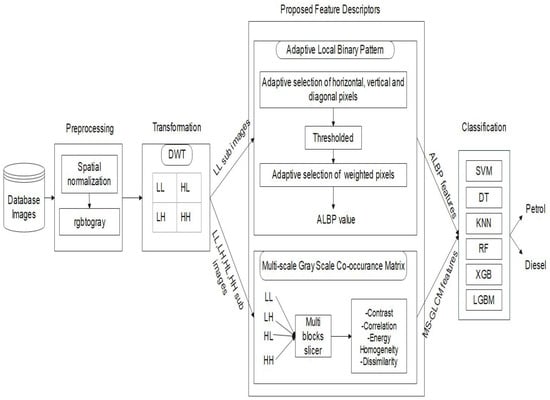
The overall flow of the proposed work is shown in Figure 1 as an architecture diagram. The proposed work consists of three main stages: (i) pre-processing, (ii) proposed feature descriptors, (iii) classification.

Figure 1. Overall proposed system architecture.

2.1. Pre-Processing

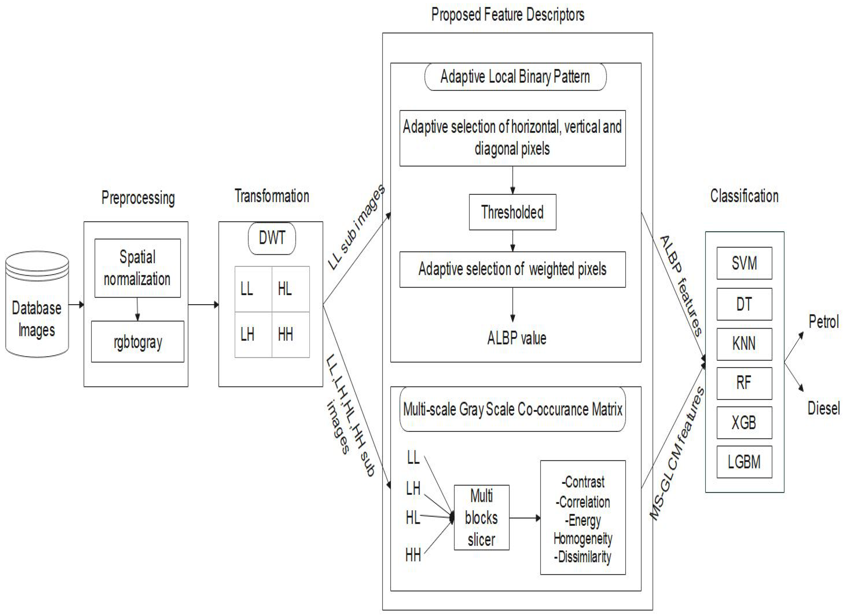
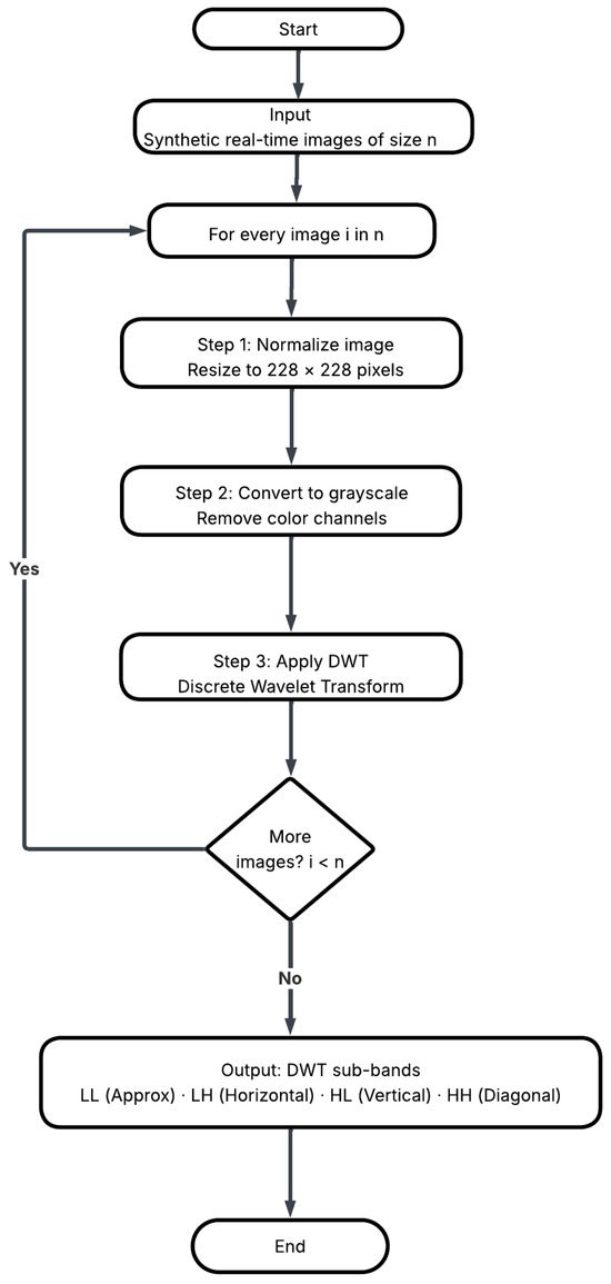
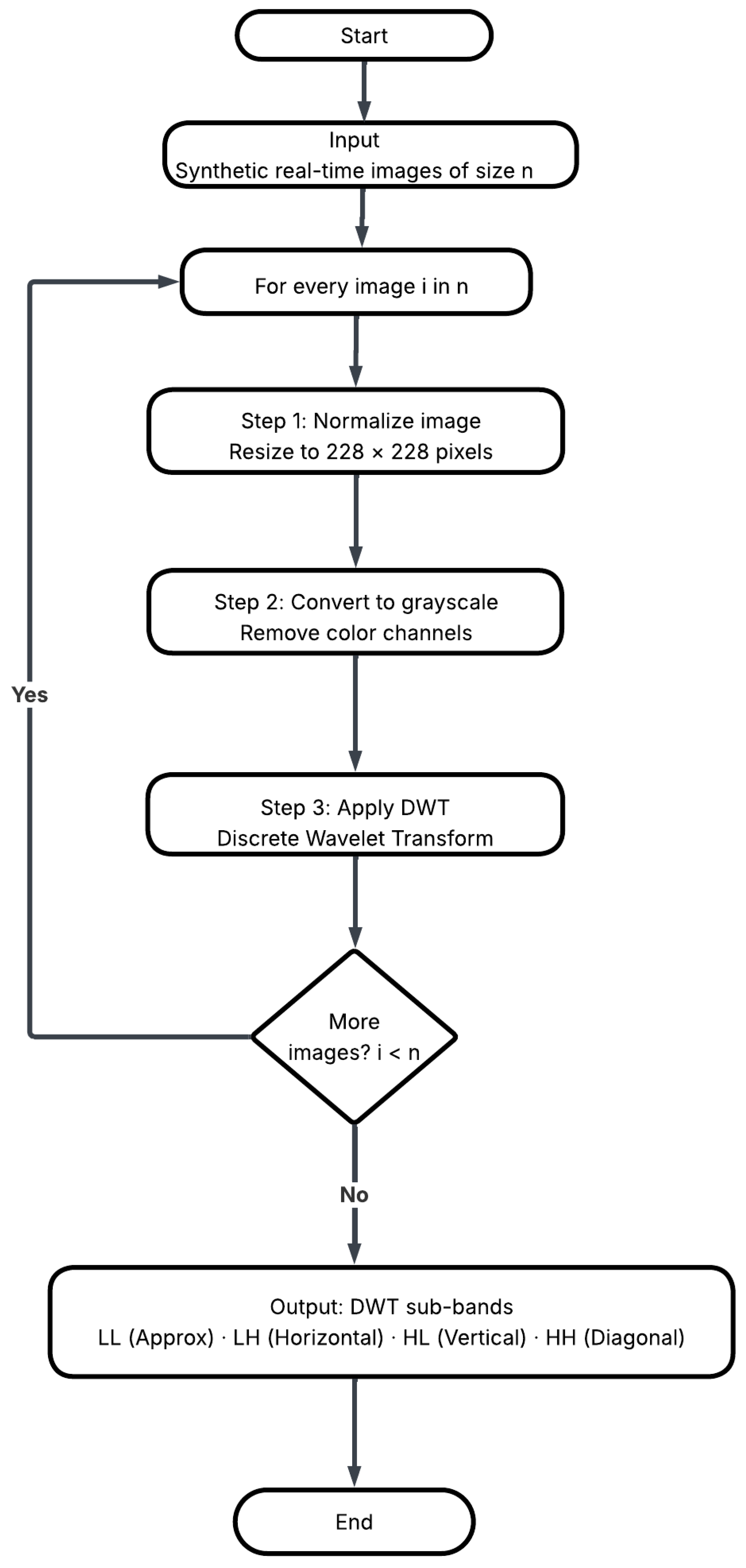
Image pre-processing is performed using three steps. Algorithm 1 explains the step-by-step procedure of image pre-processing and Figure 2 shows the detailed flowchart. The first and foremost task is to spatially normalize the input image to size 228 × 228 pixels. The spatially normalized images are converted from RGB to gray-scale images. Then, Discrete Wavelet Transform (DWT) is applied to the resultant images from the gray-scale images and decomposed into 4 different sub-bands, namely: Low-Low (LL), Low-High (LH), High-Low (HL), High-High (HH). These sub-bands are also called subimages. LL subimages are the approximate image of the original input image. LH subimages contain the information on horizontal features of the original input image. HL subimages contain the vertical features, and HH subimages contain the diagonal features. In this research, DWT helps to reduce the dimensionality of the image samples by decomposing it into multiple sub-bands with different levels of details and resolutions. This reduces the redundancy in the image samples and makes it more efficient for subsequent feature extraction.

Algorithm 1 Pre-processing
1:	Input: synthesized real-time images of size n
2:	Output: DWT subimages of LL, LH, HL, HH
3:	for every image i in n do
4:	Normalize the image to 228 × 228 pixel
5:	Convert the image into gray-scale form
6:	Transform the image using DWT
7:	end for
8:	return Approximate, Horizontal, Vertical and Diagonal sub-bands

Figure 2. Flowchart for pre-processing.

2.2. Feature Extraction

Feature extraction plays a major role in image processing while using machine learning models. The classification of image types depends on the extracted relevant features. The concept behind feature extraction is to extract essential information using shape, color, texture features, etc. The adaptive local binary pattern (ALBP) and multi-scale gray-level cooccurrence matrix (MS-GLCM) features are used in our work to extract meaningful information from subimages of DWT to train the machine learning models for the classification of fuel.

2.2.1. Adaptive Local Binary Pattern (ALBP)

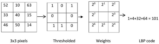
Ojala [26] introduced the LBP technique to extract the texture information in an image. The basic idea behind local binary patterns (LBPs) involves calculating the difference between a center pixel and its neighboring pixels using Equation (1). The center pixel value is taken as the threshold value. If the neighbor pixel values are greater than the threshold value, then it is replaced with value 1; else, it will be marked as 0. The resultant values taken in a clockwise direction are written as a single binary string. The extracted single binary string is converted into a decimal number. The basic LBP operator is shown in Figure 3.

Figure 3. Basic LBP operator.

In this work, $\mathrm{R}=1$ and $\mathrm{P}=8$ parameter values are used, where $\mathrm{R}$ represents radius, and $\mathrm{P}$ represents parameters. The representation of round field LBP operator with $\mathrm{R}=1$ and $\mathrm{P}=8$ is depicted in Figure 3.

$$LB{P}_{P,R}={\displaystyle \sum _{P=0}^{P-1}}s\left(g_P-g_C\right)2^P$$

(1)

where, $\mathrm{s}\left(\mathrm{x}\right)=1$ if $\mathrm{x}>0$; else, 0

In order to achieve the rotation invariant of the LBP operator,

$$LB{P}_{P,R}^{ri}=\min \left\{\mathrm{ROR}\left(LB{P}_{P,R},i\right)\right\},i=0,1,2,3,\dots ,p-1$$

(2)

where ROR in Equation (2) represents the bitwise clockwise shift rotation.

$$LB{P}_{P,R}^{ri}={\displaystyle \sum _{P=0}^{P-1}}s\left(g_P-g_C\right)\mathrm{if}U\le 2,\mathrm{otherwise}P+1$$

(3)

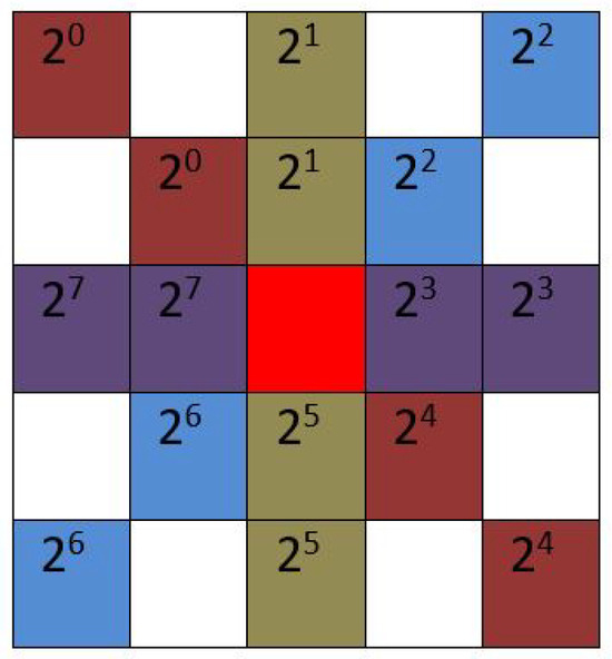
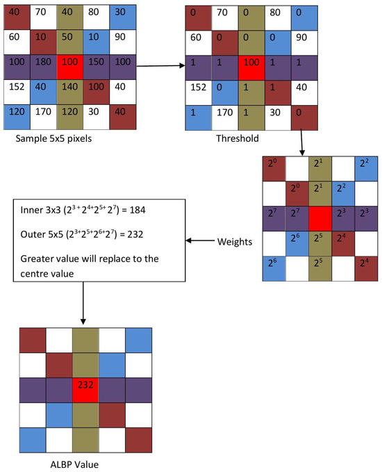
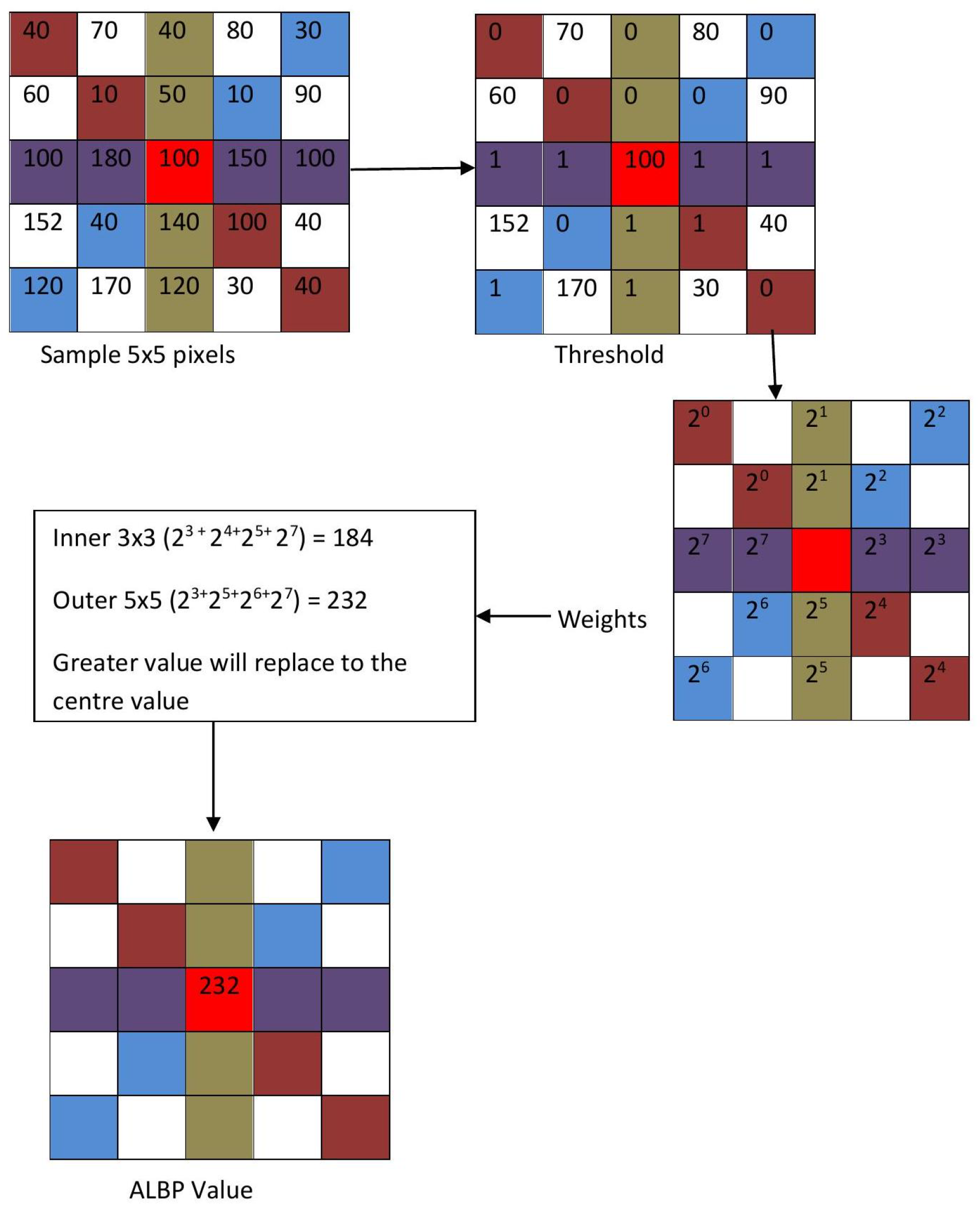
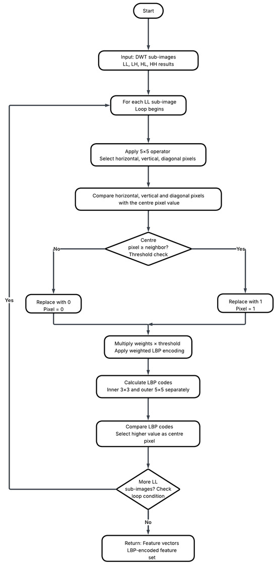
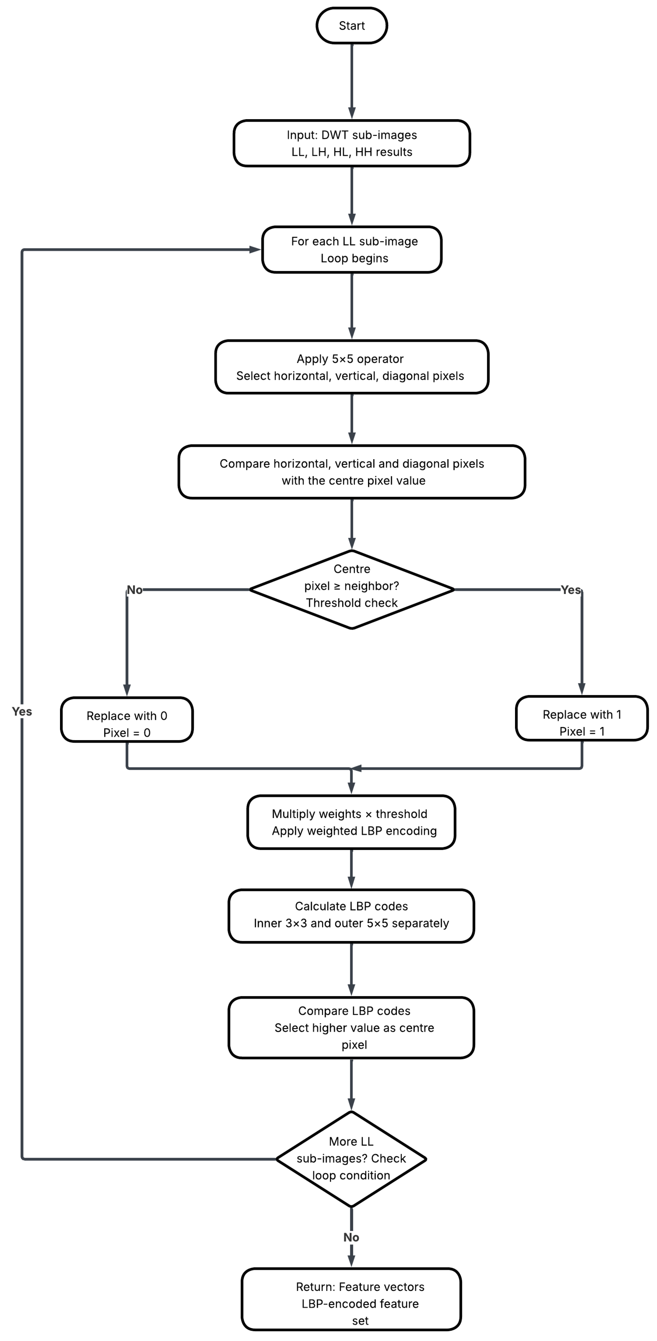
In the proposed Adaptive Local Binary Pattern (ALBP), 5 × 5 LBP operators are considered to extract the points, as shown in Figure 4. The detailed steps are given in Algorithm 2 and Figure 5.

Algorithm 2 Proposed adaptive LBP (ALBP) descriptor
1:	Input: DWT results of LL, LH, HL, HH
2:	Output: feature vectors
3:	for each LL subimage do
4:	Apply the 5 × 5 operator and select horizontal, vertical and diagonal pixels as shown in Figure 4
5:	Compare horizontal, vertical and diagonal pixels with the center pixel value
6:	if center pixel value ≥ neighbor pixel then
7:	Replace the pixel value with 1
8:	else
9:	Replace the pixel value with 0
10:	end if
11:	Multiply the weights with the threshold value
12:	Calculate the inner 3 × 3 and outer 5 × 5 operators LBP code separately
13:	Compare and choose the higher value as the center pixel of the LBP
14:	end for
15:	return Feature vectors

Figure 4. Adaptive Local Binary Pattern (ALBP) feature descriptor weights.

Figure 5. Adaptive Local Binary Pattern (ALBP) feature descriptor.

ALBP approach follows $5\times 5$ operators with an overlapping approach. The stride value is 1. Within the $5\times 5$ operator, the center pixel value is taken as the threshold. The horizontal, vertical and diagonal pixel values are compared with the center pixel value at two levels using Equation (3). At level 1, all the $3\times 3$ matrix values are taken for comparison. At level 2, 8 pixels are selected from 16 pixels. The 8 pixels location are in either horizontal or vertical or diagonal pixel values. Once the two-level layers are thresholded with the center pixels, the resultant 0’s and 1’s are multiplied with allocated weights, which are depicted in Figure 5. Level 1 is considered as inner $3\times 3$; outer is $5\times 5$. The LBP code is compared between inner versus outer, and the highest value is considered the LBP code. In Figure 5, the highest value between the inner and outer is selected and assigned as the new center pixel value. This flow is repeated for the whole set of pixel values. Figure 6 shows the detailed flowchart of the ALBP approach.

Figure 6. Flowchart for proposed Adaptive LBP (ALBP) descriptor.

2.2.2. Multi-Scale Gray-Level Co-Occurrence Matrix (MS-GLCM)

Gray-level co-occurrence matrix [13,14] is created from the gray-scale image, which calculates how often a pixel with gray-level value occurs 0° (horizontal), 90° (vertical), −45° or −135° (diagonal either bottom left to right or top left to bottom right). These angles are represented as $P_0,P_{90},P_{45},P_{135.}$ Various GLCM features can extract features. The utilized GLCM features are given below.

(a)

Contrast:

Contrast is calculated by measuring the intensity contrast between a pixel and its neighbors across the entire image [21], as defined by Equation (4). The contrast value can vary from 0 to (size(GLCM,1)-1)² [18]. In the case of an image with uniform intensity, the resulting contrast value is 1.

$$F_{\mathrm{contrast}}=\sum _{i,j}{|i-j|}^{2}P(i,j)$$

(4)

(b)

Homogeneity (similarity):

Homogeneity (Similarity) [19] is computed using Equation (5) to measure the closeness of the distribution of the pixels in the GLCM to the diagonal pixels, and the results range from 0 and 1. A diagonal GLCM has a homogeneity value of 1.

$$F_{\mathrm{Homogeneity}}=\sum _{i,j}P(i,j){\displaystyle \frac{1}{1+{(i-j)}^2}}$$

(5)

where the dissimilarity is calculated using Equation (6).

$$F_{\mathrm{Dissimilarity}}=\sum _{i,j}P(i,j)|i-j|$$

(6)

(c)

Energy:

Energy is calculated using Equation (7) from the results of the sum of squared elements in the gray-scale local co-occurrence matrix. Energy value ranges from 0 to 1.

$$F_{\mathrm{Energy}}=\sqrt{ASM}$$

(7)

where the angular second moment (ASM) [20] is calculated using Equation (8). The constant image has an energy value of 1.

$$ASM=\sum _{i,j}P{(i,j)}^2$$

(8)

(d)

Correlation:

Correlation is the measure of how a pixel is correlated to its neighbor in the given image. The correlation value ranges from $-1$ to 1, where 1 represents a positively correlated result, and $-1$ represents a negatively correlated result. Nan is the result for a constant image. The correlation is calculated using Equation (9).

$$F_{\mathrm{Correlation}}=\sum _{i,j}\frac{P(i,j)x\left(i-{\mu }_i\right)\left(j-{\mu }_j\right)}{\sqrt{{\sigma }_i^2}x{\sigma }_j^2}$$

(9)

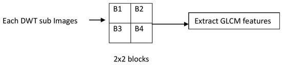
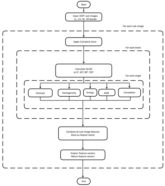
The proposed MS-GLCM feature descriptor explained in Algorithm 3 extracts the above-listed properties from a given input. The proposed model is adaptable for multi-scale object recognition and has a scale-invariant property. Each subimage from DWT is taken as input, and each subimage is divided into $4\times 4$ blocks: B1, B2, B3, B4. A total of 16 blocks are given as input to the GLCM feature extractor. Figure 7 shows the multi-scale GLCM feature descriptor. Figure 8 shows the detailed flowchart for the proposed multi-scale GLCM features.

Algorithm 3 Proposed multi-scale GLCM descriptor
1:	Input: DWT results of LL, LH, HL, HH
2:	Output: Feature Vectors
3:	for each subimage do
4:	Apply 2 × 2 block slicer
5:	for each block do
6:	Calculate GLCM in [0°, 45°, 90°, 145°]
7:	for each angle do
8:	Compute contrast using Equation (4)
9:	Compute homogeneity using Equation (5 )
10:	Compute energy using Equation (7)
11:	Computer ASM using Equation (8)
12:	Compute correlation using Equation (9)
13:	end for
14:	end for
15:	end for
16:	Combine the features of all the subimages and store them as a feature vector
17:	return Feature vectors

Figure 7. Multi-scale GLCM (MS-GLCM) approach.

Figure 8. Flowchart for proposed multi-cale GLCM descriptor.

2.3. Classification

For the ablation study, the following machine learning models were used for the empirical analysis of the classification task: support vector machine, decision tree, random forest, k-nearest neighbor, extreme gradient boosting and light gradient boosting machine [38]. The details of each model are explained below.

2.3.1. Support Vector Machine (SVM)

The SVM model is a widely used ML algorithm for the classification task. SVM can be useful for binary classification, multiclass classification and regression problems. SVM is highly successful in many applications, especially in object recognition, video analytics and text analysis. SVM aims to find a feasible solution, and it separates the classes with an optimal hyperplane. In SVM, inputs are mapped into high-dimensional space with the help of a kernel function. There are several kernel functions including Radial Basis Function (RBF), Polynomial, Gaussian, linear. Out of these kernel functions, RBF and linear kernels are widely used kernels.

2.3.2. Decision Tree (DT)

The decision tree is one of the versatile and powerful algorithms that can be used to solve a variety of problems in ML [39]. DT starts with the root node and calculates the attribute selection measure (ASM) with information gain using entropy and the Gini index. It is helpful for finding the best attribute, which is used to split the input data into subsets until all data are correctly classified.

2.3.3. Random Forest (RF)

Random forest uses multiple decision tree models and merges them to build a more accurate model. It is more reliable than DT, and it can resolve the overfitting issue. In this work, the bootstrap aggregating method was utilized in RF implementation. The bootstrap aggregating approach follows the given steps: Let us consider the number of samples in the dataset as D, and features are represented as F. Bootstrapped dataset is created by selecting random samples from D until the D in the bootstrapped set is equal to F. Each bootstrap set creates the decision tree and its model. When the unlabeled data are passed to the model, the majority voting or averaging method is used for the final prediction.

2.3.4. K-Nearest Neighbor (KNN)

KNN is a distance-based algorithm that is easy to implement and widely adopted to solve some interesting ML problems. KNN follows the lazy learning approach, where it does not involve any explicit training process; instead, it just stores the training set in memory. During testing, the unlabeled data points are classified based on the $\mathrm{K}$ number of nearest labeled data points. There are several geometrical distance metrics available, namely, Euclidean distance and Minkowski distance, to find the distance between the test data and training data.

$$\mathrm{Minkowski\_distance}\left(d_1,d_2\right)={\left({\displaystyle \sum _{i=1}^n}{\left|d_1-d_2\right|}^p\right)}^{\frac{1}{p}}$$

(10)

where Minkowski distance represents the generalized form of Manhattan and Euclidean distance with a different order $\left(p\right)$, and it is calculated using Equation (10).

$$\mathrm{Euclidean\_distance}\left(d_1,d_2\right)=\sqrt{\sum _{i=1}^n{\left(d_1-d_2\right)}^2}$$

(11)

Euclidean distance is calculated using Equation (11), where it uses the same Minkowski formula by setting the value of order $\left(p\right)=2$; thus, it is known as the $L2$-norm metric. Substituting order $\left(p\right)=1$ in Equation (10) will give the value of the Manhattan distance.

2.3.5. eXtreme Gradient Boosting (XGB)

Gradient boosting decision tree (GBDT) model is the root model. XGB is inferred from GBDT concepts, and it was proposed by Tianqi chen et al. [40]. Gradient boosting is an ensemble learning model that trains multiple weak classifiers with sequence order. The XGB algorithm aims to minimize the loss and increase the weight of the misclassified targets by calculating the negative gradients to improve further iterations in the training. The advantage of XGB with the regularization method is reduced complexity of the model, a smoother loss function and avoiding overfitting.

2.3.6. Light Gradient Boosting Machine (LGBM)

LGBM is a type of gradient boosting that is based on the decision tree algorithm. LGBM reduces memory usage and increases the efficiency of the model. The main difference between LGBM and other gradient boosting is the level-wise growth and horizontal expansion. LGBM selects the leaf that produces the least error and maximum efficiency.

2.4. Hyperparameter Tuning and Cross-Validation

Hyperparameters are the variables that control the learning process. There are two ways to find the optimal parameters. In the first method, GridsearchCV is used, and it tries all the parameter combinations. In the second method, RandomsearchCV is used, which chooses only a few random combinations out of all the available combinations.

Cross-validation is used to check the stability of the prediction model. In this work, K-fold cross-validation is used to improve the regularization of the model, where K refers to the number of partitions from the sample dataset [41]. Each time, the model fits the training set and then evaluates the test data on the trained model. Finally, the average of all the evaluation scores is used to analyze the overall method.

Performance Evaluation

The confusion matrix is used to visualize the binary classification and to calculate the True Positive (TP), True Negative (TN), False Positive (FP), and False Negative (FN). The accuracy of the classification of fuels is evaluated using Equation (12).

$$\mathrm{Accuracy}={\displaystyle \frac{TP+TN}{TP+TN+FP+FN}}$$

(12)

3. Experimental Results and Discussion

Throughout this section, the details of the experiments in the proposed work and the results on the synthesized dataset are discussed. It includes the experimental setup, dataset information, environment, parameters, and evaluation metrics.

3.1. Synthesized Dataset

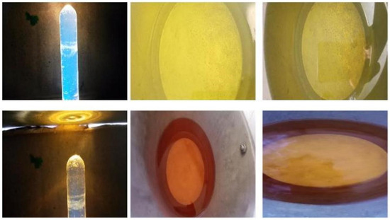
The initial samples were taken from a professional digital single lens reflex (DSLR) Sony camera in the daytime with various illuminating conditions. To analyze the importance of the illumination parameter, the samples were collected based on the illumination from direct sunlight, natural lighting inside a room and artificial lighting using a fluorescent bulb. The synthesized dataset was created using a mobile phone camera for different real-time scenarios for the task of classifying fuels. It contains two classes: diesel and petrol. This subsection describes the details of the synthesized dataset. The sample images from the synthesized dataset are shown in Figure 9. The total number of images in the datasets is 2433:1515 images are from petrol, and 918 images are from diesel samples.

Figure 9. Sample images from the synthesized dataset, categorized by fuel type: the top three images are of diesel samples, while the bottom three images are of petrol samples.

In order to improve the robustness of the models and to operate on imbalanced datasets, we used data augmentation techniques, like flipping, scaling, and rotation. These methods contribute to enhanced performance by reducing overfitting and enhancing generalization.

All the images were captured in JPEG format under various challenging scenarios such as static homogeneous background, outdoor, multi-view, different resolutions, and different viewing angles.

3.2. Experimental Setup

The experiments were carried out on a system equipped with a core i3-10105 processor and 8 gigabytes of RAM in the Windows 11 pro operating system. Python 3 programming language was utilized to implement the ablation study, and several libraries were employed, including pandas-1.0.5, numpy-1.17.3, scikit-learn-0.20, and OpenCV-3.1.0. The proposed hybrid ALBP–MS-GLCM features were compared with the state-of-the-art feature descriptors like LBP-only approach [27], GLCM-only approach [14], Hybrid LBP–GLCM approach [15].

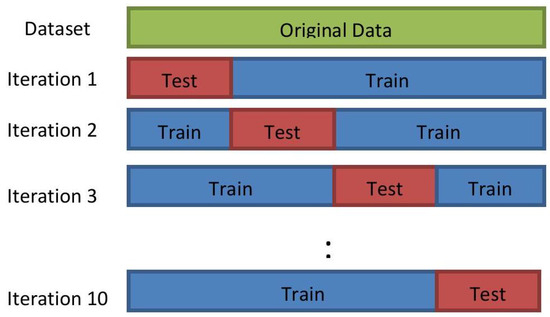
The proposed method involves several steps, including spatial normalization of input images to a 224 × 224 pixel size and conversion of RGB images into gray-scale images. DWT is then applied to each image, and features are extracted using a fusion of LBP and GLCM features. The classification accuracy of six different models, including SVM, RF, KNN, DT, XGB, and LGBM, is evaluated using GridSearchCV and RandomSearchCV parameters with 10-fold cross-validation. The details of the hyperparameters for each ML model are shown in Table 1. The 10-fold cross-validation visual representation is depicted in Figure 10 for better understanding. Notably, in the 10-fold cross-validation approach, the ten test predictions are averaged to derive the final result.

Table 1. Parameters used in GridSearchCV and RandomSearchCV and chosen hyperparameters for each machine learning model.

ML Model	Hyperparameters	Values	RandomSearchCV	GridSearchCV
SVM	C	[0.1, 10, 100, 1000]	0.1	0.1
	Gamma	[1, 0.1, 0.01, 0.001]	0.1	0.1
	Kernel	[rbf, linear]	rbf	rbf
DT	Max_depth	[2, 3, 5, 10, 20]	3	3
	Min_leaf	[5, 10, 20, 50]	20	20
	Criterion	[‘Gini’, ‘Entropy’]	Entropy	Entropy
RF	N_estimators	[10, 50, 100]	50	50
	Max_features	[‘auto’, ‘log2’, ‘sqrt’]	sqrt	sqrt
	Bootstrap	[‘True’, ‘False’]	True	True
	Max_depth	[3, 5, 6, 7, 8]	5	5
	Min_sample_split	[5, 6, 7, 8]	7	8
K-NN	Leaf_size	[3, 4, 5, 6, 7, 8, 9]	6	6
	N_neighbours	[1, 2, 3, 4, 5, 6, 7]	4	4
	Weights	[‘uniform’, ‘distance’]	uniform	uniform
XGB	Learning_rate	[0.01, 0.1]	0.01	0.01
	Max_depth	[3, 5, 7, 10]	7	7
	Minchildweight	[1, 3, 5]	3	3
	Subsample	[0.5, 0.7]	0.5	0.5
	N_estimators	[100, 200, 500]	200	100
	Objective	[‘reg’, ‘squarederror’]	squarederror	squarederror
	Max_features	[7, 8, 9, 10]	9	9
LGBM	Max_depth	[8, 10, 15]	10	10
	Learning_rate	[0.001, 0.01, 0.012]	0.01	0.012
	Num_leaves	[80, 100, 200]	100	100
	N_estimators	[200, 250]	250	250

Figure 10. Ten-fold cross-validation visual representation.

The values of precision, recall and F1 score are 0.9505, 0.9600, and 0.9552, respectively, for the proposed approach applied on the synthesized dataset.

Deep learning technique ensemble upgraded, which is a combination of Upgraded ResNet152V2, Upgraded InceptionResNetV2, and Upgraded EfficientNetB7 produced a recall, precision and F1 score of 99.54, 99.69 and 99.62, respectively.

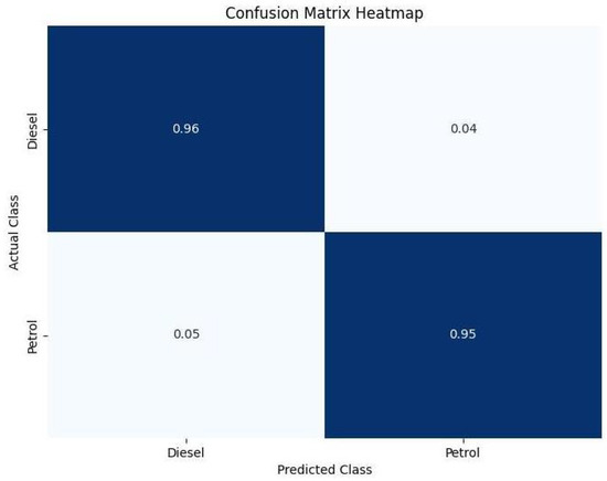
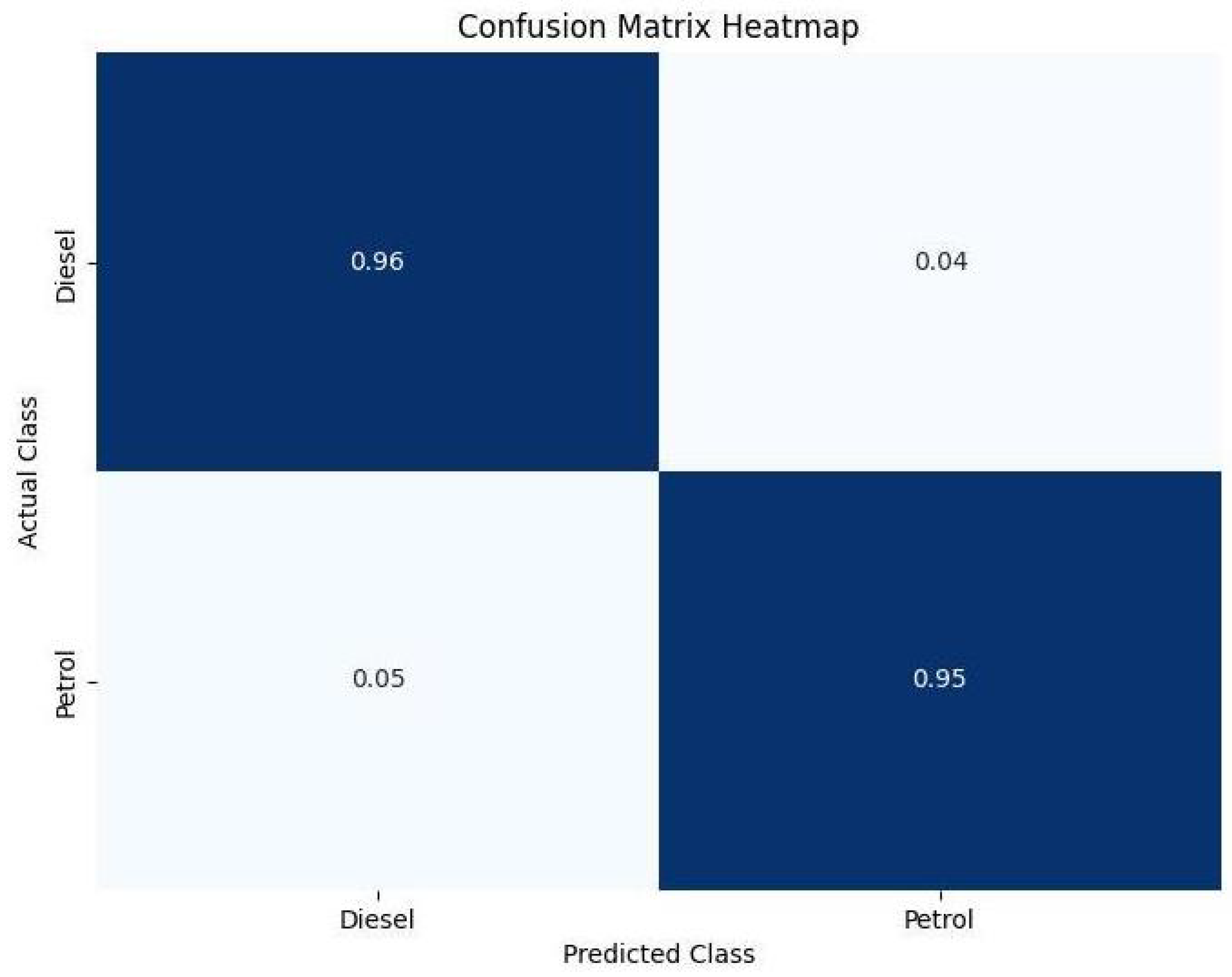
In the same way, we analyzed all six machine learning models listed above. The confusion matrix of the proposed approach run on the synthesized dataset is shown in Figure 11.

Figure 11. Confusion matrix of proposed approach applied on synthesized dataset.

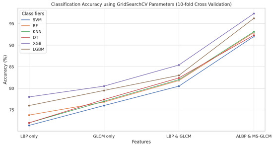
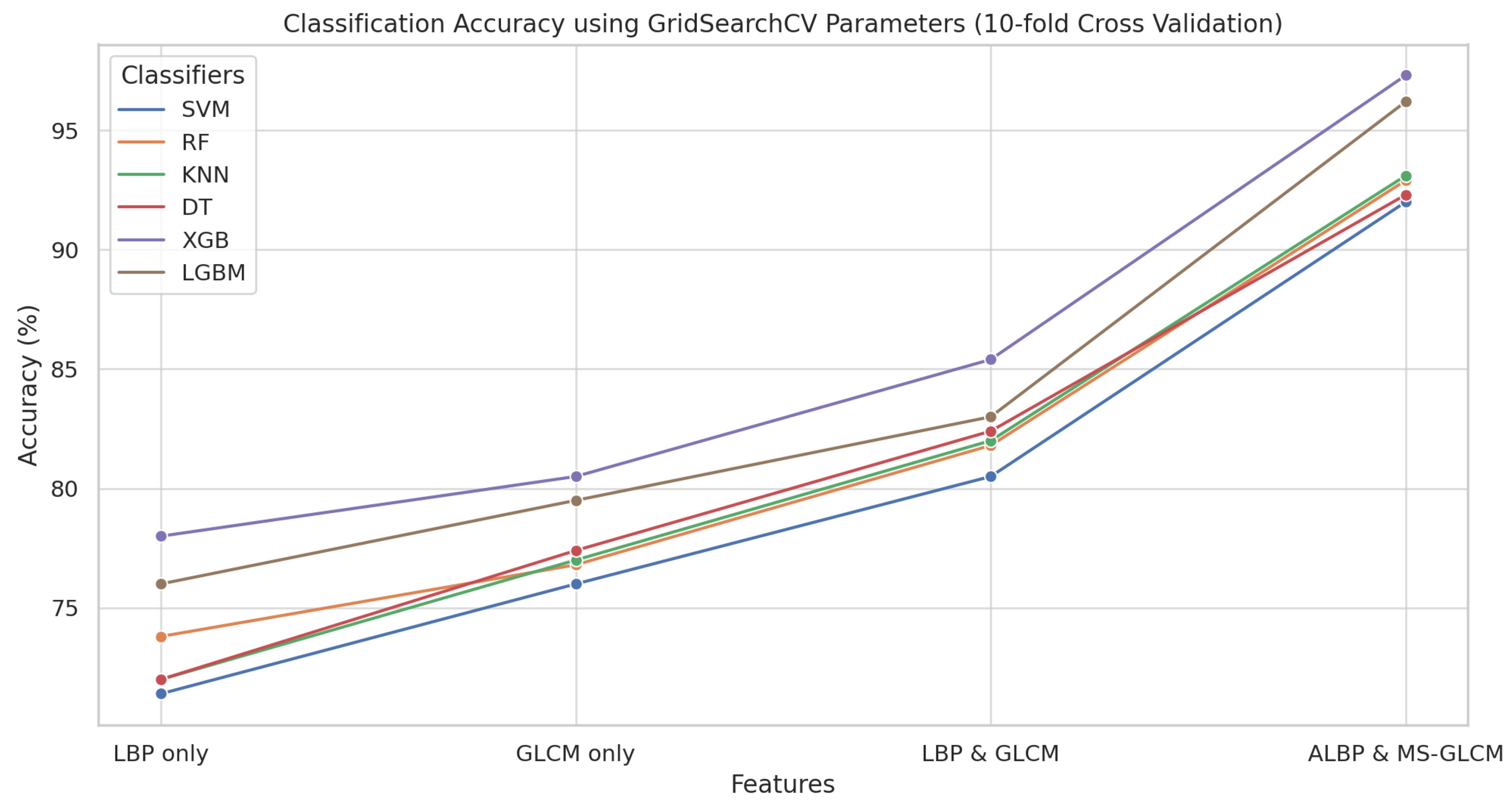
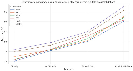
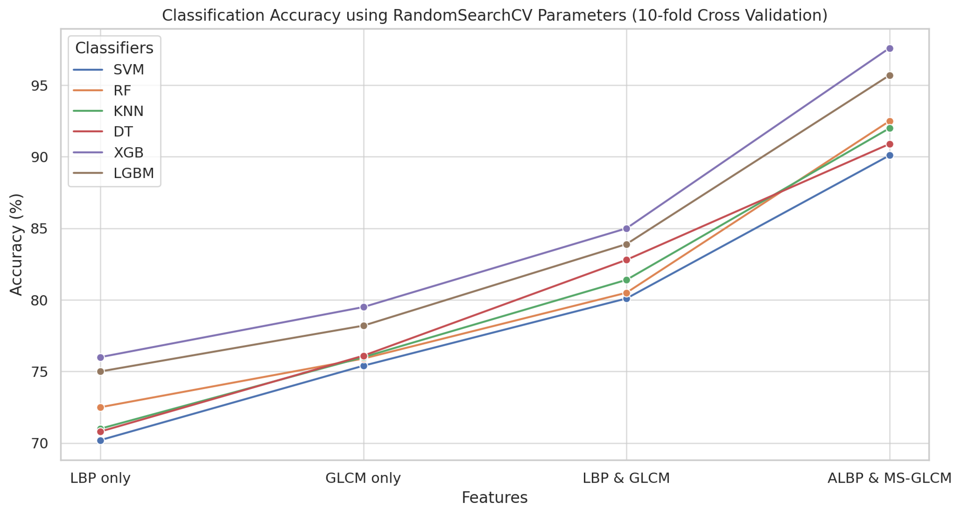
The performance evaluation metric, i.e., classification accuracy of the ML models, is shown in Table 2 and Table 3. In this ablation study, LBP and GLCM descriptors were individually analyzed with the ML models and then the fusion of LBP and GLCM descriptors without DWT transform was taken into consideration. Finally, the hybrid LBP and GLCM descriptors with DWT components were considered for evaluation. As per the results in Figure 12 and Figure 13, the XGB model achieved better accuracy than the other classifiers.

Table 2. Classification accuracy using GridSearchCV parameters (in %) using 10-fold cross validation.

Classifiers	LBP Only	GLCM Only	LBP & GLCM	ALBP & MS-GLCM
SVM	71.4	76	80.5	92
RF	73.8	76.8	81.8	92.9
KNN	72	77	82	93.1
DT	72	77.4	82.4	92.3
XGB	78	80.5	85.4	97.3
LGBM	76	79.5	83	96.2

Table 3. Classification accuracy using RandomSearchCV parameters (in %) using 10-fold cross validation.

Classifiers	LBP Only	GLCM Only	LBP & GLCM	ALBP & MS-GLCM
SVM	70.2	75.4	80.1	90.1
RF	72.5	75.9	80.5	92.5
KNN	71	76	81.4	92
DT	70.8	76.1	82.8	90.9
XGB	76	79.5	85	97.6
LGBM	75	78.2	83.9	95.7

Figure 12. Classification accuracy using GridSearchCV parameters (10-fold Cross Validation).

Figure 13. Classification Accuracy using RandomSearchCV Parameters (10-fold cross-validation).

4. Conclusions and Future Work

In this work, we performed an ablation study on fuel adulteration by integrating different feature descriptors and modeled it with different $\mathrm{ML}$ algorithms.

To provide a more in-depth analysis, the hyperparameters of the ML models were adjusted to fine tune the results based on grid search and random search. In this ablation study, the XGB model achieved $97.6$% accuracy using ALBP and MS-GLCM feature descriptors on the synthesized dataset.

The data were acquired in a controlled environment, which may impact the generalizability of the ML models.

Future works are planned to include more challenging scenarios in a controlled environment for image acquisition.

References

- Team, I. What Percentage of the Global Economy Is the Oil and Gas Drilling Sector? 2022. Available online: https://www.investopedia.com/ask/answers/030915/what-percentage-global-economy-comprised-oil-gas-drilling-sector.asp (accessed on 4 January 2023).
- Hemachandiran, S.; Aghila, G.; Siddharth, R. Automation to Find Adulteration in Downstream Petroleum Monitoring Using Machine Learning: An Overview. In Proceedings of the Recent Advances in Manufacturing, Automation, Design and Energy Technologies; Natarajan, S.K., Prakash, R., Sankaranarayanasamy, K., Eds.; Springer Nature: Berlin/Heidelberg, Germany, 2022; pp. 415–423. [Google Scholar]
- Li, J.; Allinson, N.M. A comprehensive review of current local features for computer vision. Neurocomputing 2008, 71, 1771–1787. [Google Scholar] [CrossRef]
- Kazmi, W.; Garcia-Ruiz, F.; Nielsen, J.; Rasmussen, J.; Andersen, H.J. Exploiting affine invariant regions and leaf edge shapes for weed detection. Comput. Electron. Agric. 2015, 118, 290–299. [Google Scholar] [CrossRef]
- Chen, W.T.; Liu, W.C.; Chen, M.S. Adaptive Color Feature Extraction Based on Image Color Distributions. IEEE Trans. Image Process. 2010, 19, 2005–2016. [Google Scholar] [CrossRef] [PubMed]
- Atlam, H.F.; Attiya, G.; El-fishawy, N. Comparative Study on CBIR based on Color Feature. Int. J. Comput. Appl. 2013, 78, 9–15. [Google Scholar] [CrossRef]
- Ojala, T.; Pietikäinen, M.; Harwood, D. A comparative study of texture measures with classification based on featured distributions. Pattern Recognit. 1996, 29, 51–59. [Google Scholar] [CrossRef]
- Patel, M.N.; Tandel, P. Article: A Survey on Feature Extraction Techniques for Shape based Object Recognition. Int. J. Comput. Appl. 2016, 137, 16–20. [Google Scholar]
- Krithika, L.B.; Priya, G.G.L. Graph based feature extraction and hybrid classification approach for facial expression recognition. J. Ambient. Intell. Humaniz. Comput. 2021, 12, 2131–2147. [Google Scholar] [CrossRef] [PubMed]
- Rosten, E.; Porter, R.; Drummond, T. Faster and Better: A Machine Learning Approach to Corner Detection. IEEE Trans. Pattern Anal. Mach. Intell. 2010, 32, 105–119. [Google Scholar] [CrossRef] [PubMed]
- van de Weijer, J.; Gevers, T.; Geusebroek, J.M. Edge and corner detection by photometric quasi-invariants. IEEE Trans. Pattern Anal. Mach. Intell. 2005, 27, 625–630. [Google Scholar] [CrossRef] [PubMed]
- Humeau-Heurtier, A. Texture Feature Extraction Methods: A Survey. IEEE Access 2019, 7, 8975–9000. [Google Scholar] [CrossRef]
- Veerashetty, S.; Virupakshappa; Ambika. Face recognition with illumination, scale and rotation invariance using multiblock LTP-GLCM descriptor and adaptive ANN. Int. J. Syst. Assur. Eng. Manag. 2022, 15, 174–187. [Google Scholar] [CrossRef]
- Khan, S.U.; Islam, N.; Jan, Z.; Haseeb, K.; Shah, S.I.A.; Hanif, M. A machine learning-based approach for the segmentation and classification of malignant cells in breast cytology images using gray level co-occurrence matrix (GLCM) and support vector machine (SVM). Neural Comput. Appl. 2022, 34, 8365–8372. [Google Scholar] [CrossRef]
- Öztürk, Ş.; Akdemir, B. Application of Feature Extraction and Classification Methods for Histopathological Image using GLCM, LBP, LBGLCM, GLRLM and SFTA. Procedia Comput. Sci. 2018, 132, 40–46. [Google Scholar] [CrossRef]
- Hu, S.; Pan, Z.; Dong, J.; Ren, X. A Novel Adaptively Binarizing Magnitude Vector Method in Local Binary Pattern Based Framework for Texture Classification. IEEE Signal Process. Lett. 2022, 29, 852–856. [Google Scholar] [CrossRef]
- Roy, H.; Bhattacharjee, D.; Krejcar, O. Interpretable Local Frequency Binary Pattern (LFrBP) Based Joint Continual Learning Network for Heterogeneous Face Recognition. IEEE Trans. Inf. Forensics Secur. 2022, 17, 2125–2136. [Google Scholar] [CrossRef]
- Yuan, J.H.; Huang, D.S.; Zhu, H.D.; Gan, Y. Completed hybrid local binary pattern for texture classification. In Proceedings of the 2014 International Joint Conference on Neural Networks (IJCNN), Beijing, China, 6–11 July 2014; pp. 2050–2057. [Google Scholar] [CrossRef]
- Fan, K.C.; Hung, T.Y. A Novel Local Pattern Descriptor—Local Vector Pattern in High-Order Derivative Space for Face Recognition. IEEE Trans. Image Process. 2014, 23, 2877–2891. [Google Scholar] [CrossRef] [PubMed]
- Zhang, B.; Gao, Y.; Zhao, S.; Liu, J. Local Derivative Pattern Versus Local Binary Pattern: Face Recognition With High-Order Local Pattern Descriptor. IEEE Trans. Image Process. 2010, 19, 533–544. [Google Scholar] [CrossRef] [PubMed]
- Karis, M.S.; Razif, N.R.A.; Ali, N.M.; Rosli, M.A.; Aras, M.S.M.; Ghazaly, M.M. Local Binary Pattern (LBP) with application to variant object detection: A survey and method. In Proceedings of the 2016 IEEE 12th International Colloquium on Signal Processing & Its Applications (CSPA), Melaka, Malaysia, 4–6 March 2016; pp. 221–226. [Google Scholar] [CrossRef]
- Deng, W.; Hu, J.; Guo, J. Compressive Binary Patterns: Designing a Robust Binary Face Descriptor with Random-Field Eigenfilters. IEEE Trans. Pattern Anal. Mach. Intell. 2019, 41, 758–767. [Google Scholar] [CrossRef] [PubMed]
- Qiang, Z.; Jianhua, A.; Xiaoya, S.; Sunyan, H. Extended complete local binary pattern for texture classification. Multimed. Tools Appl. 2022, 81, 5389–5405. [Google Scholar] [CrossRef]
- Hu, X.; Li, G. Temporal Tensor Local Binary Pattern: A Novel Local Tensor Time Series Descriptor. IEEE Trans. Ind. Inform. 2020, 16, 6393–6402. [Google Scholar] [CrossRef]
- Nguyen, V.D.; Nguyen, D.D.; Nguyen, T.T.; Dinh, V.Q.; Jeon, J.W. Support Local Pattern and its Application to Disparity Improvement and Texture Classification. IEEE Trans. Circuits Syst. Video Technol. 2014, 24, 263–276. [Google Scholar] [CrossRef]
- Ojala, T.; Pietikainen, M.; Maenpaa, T. Multiresolution gray-scale and rotation invariant texture classification with local binary patterns. IEEE Trans. Pattern Anal. Mach. Intell. 2002, 24, 971–987. [Google Scholar] [CrossRef]
- Zhao, G.; Pietikainen, M. Dynamic Texture Recognition Using Local Binary Patterns with an Application to Facial Expressions. IEEE Trans. Pattern Anal. Mach. Intell. 2007, 29, 915–928. [Google Scholar] [CrossRef] [PubMed]
- Zhang, W.; Shan, S.; Gao, W.; Chen, X.; Zhang, H. Local Gabor binary pattern histogram sequence (LGBPHS): A novel non-statistical model for face representation and recognition. In Proceedings of the Tenth IEEE International Conference on Computer Vision (ICCV’05), Beijing, China, 17–20 October 2005; Volume 1, pp. 786–791. [Google Scholar] [CrossRef]
- Wang, W.; Jiang, Y.; Wang, G.; Guo, F.; Li, Z.; Liu, B. Multi-Scale LBP Texture Feature Learning Network for Remote Sensing Interpretation of Land Desertification. Remote Sens. 2022, 14, 3486. [Google Scholar] [CrossRef]
- Zhu, J.; Zhang, W. Application of Improved DNN Algorithm Based on Feature Fusion in Fine-Grained Image Recognition. IEEE Access 2024, 12, 32140–32151. [Google Scholar] [CrossRef]
- Zhang, D.; Pang, W.; Wang, K.; Yang, F.; Zhang, J. Tongue Coating Grading Identification Using Deep Learning for Hyperspectral Imaging Data. IEEE Access 2023, 11, 93151–93159. [Google Scholar] [CrossRef]
- Wang, L.; Zhang, H.; Zhang, Y.; Hu, K.; An, K. A Deep Learning-Based Experiment on Forest Wildfire Detection in Machine Vision Course. IEEE Access 2023, 11, 32671–32681. [Google Scholar] [CrossRef]
- Chen, Y.; Zhang, H.; Yan, W.; Zhang, X.; Jiang, Z.; Liu, Y. A multi-dimensional data integration approach for machining system multi-level energy consumption modeling and prediction. Int. J. Comput. Integr. Manuf. 2026, 39, 245–266. [Google Scholar]
- Alazemi, F.; Alazmi, A.; Alrumaidhi, M.; Molden, N. Predicting fuel consumption and emissions using GPS-based machine learning models for gasoline and diesel vehicles. Sustainability 2025, 17, 2395. [Google Scholar] [CrossRef]
- Josef, L.; Kawlni, L.; Lawmawmi, L.; Thanga, H. Exploration of various chemometric methods for analysis of gasoline adulteration. Next Res. 2026, 8, 101608. [Google Scholar] [CrossRef]
- Sobreira, P.J.M.B.; Filho, A.C.L.; de Lucena, J.A.; Belo, F.A. Detection of adulteration in gasoline blends with ethanol via machine learning and infrared images. Proc. Inst. Mech. Eng. Part D J. Automob. Eng. 2026, 2026, 09544070261443453. [Google Scholar] [CrossRef]
- Babu, V.; Krishna, R.; Mani, N. Review on the Detection of Adulteration in Fuels through Computational Techniques. Mater. Today Proc. 2017, 4, 1723–1729. [Google Scholar] [CrossRef]
- Kumari, R.; Srivastava, S.K. Machine Learning: A Review on Binary Classification. Int. J. Comput. Appl. 2017, 160, 11–15. [Google Scholar] [CrossRef]
- Baashar, Y.; Alkawsi, G.; Ali, N.; Alhussian, H.; Bahbouh, H.T. Predicting student’s performance using machine learning methods: A systematic literature review. In Proceedings of the 2021 International Conference on Computer & Information Sciences (ICCOINS), Virtual, 13–15 July 2021; pp. 357–362. [Google Scholar] [CrossRef]
- Chen, T.; Li, H.; Yang, Q.; Yu, Y. General Functional Matrix Factorization Using Gradient Boosting. In Proceedings of the 30th International Conference on Machine Learning, Atlanta, GA, USA, 17–19 June 2013; Proceedings of Machine Learning Research; Dasgupta, S., McAllester, D., Eds.; PMLR: Cambridge, MA, USA, 2013; Volume 28, pp. 436–444. [Google Scholar]
- Khan, M.A.; Zafar, A.; Farooq, F.; Javed, M.F.; Alyousef, R.; Alabduljabbar, H.; Khan, M.I. Geopolymer Concrete Compressive Strength via Artificial Neural Network, Adaptive Neuro Fuzzy Interface System, and Gene Expression Programming With K-Fold Cross Validation. Front. Mater. 2021, 8, 621163. [Google Scholar] [CrossRef]
Disclaimer/Publisher’s Note: The statements, opinions and data contained in all publications are solely those of the individual author(s) and contributor(s) and not of MDPI and/or the editor(s). MDPI and/or the editor(s) disclaim responsibility for any injury to people or property resulting from any ideas, methods, instructions or products referred to in the content. |
© 2026 by the authors. Licensee MDPI, Basel, Switzerland. This article is an open access article distributed under the terms and conditions of the Creative Commons Attribution (CC BY) license.