AMI-Informed Hierarchical Deep Reinforcement Learning–Model Predictive Control for Coordinated EV, PV, and Battery Energy Management in Campus Microgrids

Abstract

This paper proposes an advanced metering infrastructure (AMI)-informed hierarchical energy management framework for coordinated operation of electric vehicles (EVs), photovoltaic (PV) systems, and battery energy storage systems (BESS) in campus microgrids. The proposed two-layer architecture integrates a soft actor–critic (SAC) deep reinforcement learning (DRL) agent in the upper layer with a receding horizon model predictive control (MPC) optimizer in the lower layer. The key novelty is an AMI-to-control pipeline that transforms historical 15 min smart-meter measurements into operational flexibility features and embeds them into a hierarchical SAC–MPC architecture, where the DRL layer provides adaptive coordination and the MPC layer enforces grid, storage, and EV-service constraints. The proposed framework using the real-world Pecan Street data (15 min resolution) of 73 homes across Austin, Texas and California (2014–2019) achieves a 53.1% cost reduction and a 25.7% peak demand reduction when compared with uncontrolled charging, and the proposed framework outperforms MPC-only (50.9%), DRL-only (−5.2%), and rule-based (5.1%) baselines. The statistically significant contributions of network-aware constraints, demand-response activation, and predictive look-ahead horizon are statistically significant (n = 10 independent runs) contributions (p = 0.001). The state representation informed by AMI offers directional cost improvement (+8.4%, p = 0.055) with 11% faster convergence of training. The zero network constraint violation is observed in all evaluation scenarios and the average MPC solve time is around 150 ms, which is much less than the 15 min sampling period. Sensitivity analyses show that the hierarchical DRL–MPC architecture remains computationally feasible across EV penetration, seasonal, and forecast-uncertainty scenarios. However, BESS provided no net economic benefit under the evaluated energy-only TOU tariff, increasing weekly cost by $15.25 and peak grid demand by 14.2 kW. Break-even analysis indicates that demand charges of approximately $9.9/kW per month are required for BESS to become cost-effective in the proxy system, highlighting that storage value depends strongly on tariff design and peak-demand objective formulation.

1. Introduction

The high rate of electric vehicle (EV) proliferation, which has distributed photovoltaic (PV) generation and battery energy storage systems (BESS) in institutional and campus settings, is fundamentally altering the operating environment of distribution networks. Small-scale microgrids, with their heterogeneous and predictable load profiles, high EV adoption rates, and high rooftop PV penetration, are a perfect testbed of intelligent energy management systems. Nonetheless, the concomitant optimization of EV charging schedules, PV self-consumption, BESS dispatch, and demand response under time-varying electricity tariffs and network constraints constitutes a high-dimensional, non-linear, and stochastic control problem that is beyond the ability of traditional rule-based or simply model-based methods [1].

The deployment of advanced metering infrastructure (AMI) in the current distribution networks produces fine-grained 15 min resolution data streams that capture household load patterns, EV-charging behavior, PV generation, and voltage signatures [2]. Although such information is readily available, most current energy management frameworks do not view AMI data as a real-time operation input but, instead, as a post-hoc analysis tool [3]. The gap that exists between these two branches of research is bridged in this paper, through the proposal of a framework that explicitly encodes AMI-derived flexibility features, such as EV flexibility envelopes, PV availability indices, and load deferral fractions, into the state space of a deep reinforcement learning agent, allowing the agent to learn anticipatory coordination strategies tuned to the specific flexibility characteristics of each connected asset.

The basic conflict that is being addressed in this work is the inherent tension between two complementary requirements: (i) adaptive optimality, where the control strategy must respond dynamically in response to uncertain renewable generation and stochastic EV arrival/departure patterns, and (ii) constraint satisfaction, where voltage limits, feeder capacity limits, BESS state-of-charge constraints, and EV service quality requirements must be imposed at all times. Neither standalone DRL nor standalone MPC can fulfill both requirements simultaneously: DRL without MPC constraints will have unconstrained optimization behavior which can result in network limits being violated (as we have found in our results showing that DRL-only incurs 5.2% additional cost compared with uncontrolled operation due to the lack of unscheduled peak charging), while MPC without DRL adaptation relies on constant coordination parameters which cannot exploit the full flexibility potential revealed by AMI data.

To resolve this tension, we propose a hierarchical two-layer architecture in which a trained SAC agent (upper layer) generates AMI-informed coordination signals every 15 min, which are passed to an 8 h receding-horizon CVXPY-based MPC optimizer (lower layer) that solves the constrained dispatch problem with hard guarantees on voltage, feeder, and BESS limits. The framework is trained and evaluated on the Pecan Street Dataport dataset—one of the most comprehensive real-world residential AMI datasets available—comprising 73 homes across Austin, Texas and California over a five-year period (2014–2019).

Main Contributions

This paper makes the following contributions:

• AMI-to-flexibility feature construction: A reproducible AMI feature-extraction layer is developed to convert historical 15 min smart-meter measurements into operational flexibility indicators, including EV upward/downward flexibility, PV availability, load deferral fraction, charging-window start, and charging-window remaining. Unlike approaches that use AMI data only for forecasting or post-hoc analysis, the proposed method embeds AMI-derived flexibility directly into the online control state.
• Hierarchical DRL–MPC control architecture: A two-layer energy-management framework is proposed in which a soft actor–critic (SAC) agent generates high-level coordination signals, including EV priority, BESS reserve margin, PV curtailment allowance, and demand-response activation, while a lower-level receding-horizon MPC optimizer converts these signals into feasible dispatch decisions.
• Constraint-aware multi-resource coordination: The framework jointly coordinates EV charging, PV utilization, BESS dispatch, and demand response while enforcing operational constraints on feeder import, voltage magnitude, BESS state of charge, BESS power, and EV service requirements. This design addresses the complementary weaknesses of standalone DRL and standalone MPC: DRL provides adaptive coordination under uncertainty, while MPC provides constraint-aware dispatch.
• Campus-like microgrid validation using real AMI data: A three-zone campus-proxy microgrid is calibrated using real Pecan Street AMI statistics from 73 homes across Austin, Texas and California, including measured load, EV, PV, and voltage profiles. This provides a data-grounded testbed for evaluating coordinated EV–PV–BESS control under realistic 15 min temporal variability.
• Component-level ablation and sensitivity analysis: The proposed architecture is evaluated against uncontrolled charging, rule-based EMS, MPC-only, DRL-only, and forecast-then-optimize baselines. Additional ablation and sensitivity studies isolate the contributions of AMI features, network constraints, MPC look-ahead, demand response, BESS configuration, EV penetration, seasonal variation, and forecast uncertainty.

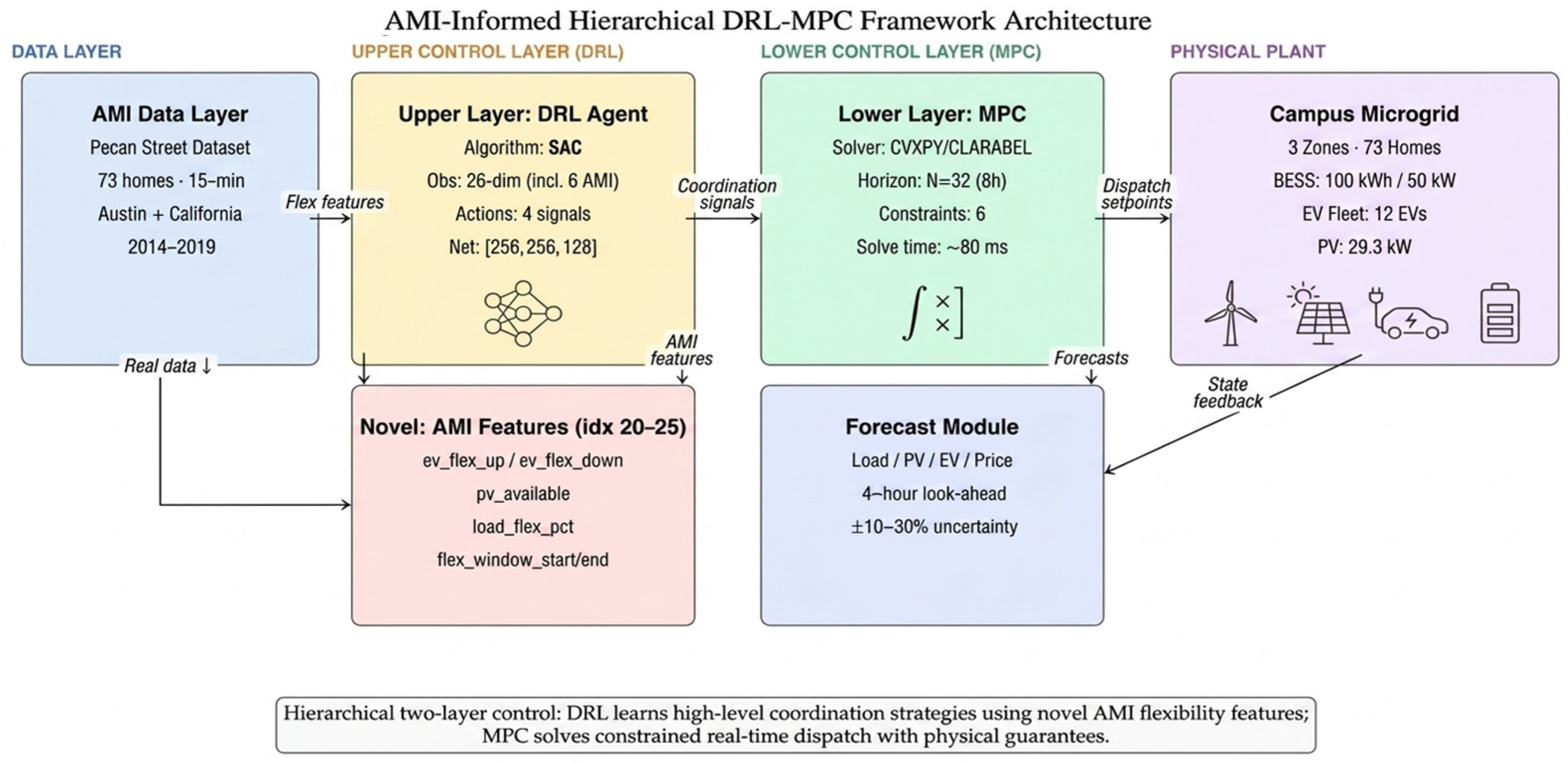
Figure 1 summarizes the proposed AMI-to-control workflow and clarifies the separation of roles between the learning and optimization layers. The AMI layer first converts historical 15 min smart-meter measurements into operational flexibility features, which allow the SAC agent to generate adaptive coordination signals rather than direct physical dispatch commands. These signals are then passed to the MPC layer, which computes feasible EV, PV, BESS, and demand-response decisions while enforcing network and asset constraints. This architecture provides the basis for the literature comparison in the next section, where existing AMI-based, MPC-based, DRL-based, and hybrid EMS approaches are reviewed against the proposed control structure.

Figure 1. System architecture: hierarchical DRL–MPC two-layer framework. Arrows indicate data flow, AMI-feature transfer, coordination-signal exchange, forecast input, dispatch setpoints, and state feedback among the framework layers.

2. Related Work

The problem of coordinated energy management in microgrids integrating electric vehicles (EVs), photovoltaic (PV) systems, and battery energy storage systems (BESS) has attracted substantial research attention over the past decade. Prior contributions span three largely parallel streams: (i) model-based optimization and MPC methods applied to campus and institutional microgrids; (ii) deep reinforcement learning (DRL) approaches that learn near-optimal dispatch policies without explicit system models; and (iii) emerging hybrid frameworks that combine DRL with MPC to achieve both adaptability and constraint satisfaction. The role of advanced metering infrastructure (AMI) as a real-time operational input—rather than merely a monitoring or post-hoc analysis tool—remains underexplored across all three streams. The following subsections review each area, identify the specific gaps that motivate the proposed framework, and position the proposed work relative to the current state of the art. Table 1 summarizes the positioning across all major EMS research streams.

Table 1. Positioning of the proposed framework relative to major EMS research streams.

Study Category	AMI-Derived Flexibility	DRL	MPC	EV	PV	BESS	Network Constraints	Campus Setting	Gap
AMI-based EMS	Yes/partial	No	Sometimes	Partial	Partial	Partial	Limited	Rare	Uses AMI mainly for monitoring/forecasting
DRL EV/PV scheduling	No/limited	Yes	No	Yes	Yes	Sometimes	Weak	Rare	Adaptive but lacks hard feasibility
MPC campus microgrids	No/limited	No	Yes	Yes	Yes	Yes	Yes	Yes	Constraint-aware but fixed/adaptation-limited
Hybrid DRL–MPC	Rare	Yes	Yes	Often	Sometimes	Sometimes	Partial	Rare	Usually not AMI-informed or campus-focused
Proposed framework	Yes	Yes	Yes	Yes	Yes	Yes	Yes	Campus-proxy	AMI-to-flexibility + SAC supervision + constrained MPC

2.1. Rule-Based and Optimization-Based Energy Management

Conventional energy management systems (EMS) for microgrids are based on rule-guided heuristics or deterministic optimization [4]. Rule-based methods are computationally efficient but require expert-designed decision rules that cannot adapt to the stochastic nature of renewable generation and time-varying EV demand [5]. Linear and mixed-integer programming formulations achieve global optimality under perfect forecast conditions but become highly suboptimal as uncertainty increases [6].

Model predictive control (MPC) addresses forecast uncertainty through receding-horizon re-optimization, and has emerged as the dominant formulation for campus and institutional microgrids. Achour et al. [7] demonstrated an MPC-based demand-response scheme for peak shaving in a smart campus microgrid integrating PV, BESS, and EVs with AMI-based measurement infrastructure—the closest directly comparable system architecture to the present work. Ouammi [8] proposed MPC scheduling frameworks for peak load reduction in institutional building microgrids exploiting vehicle-to-building (V2B) concepts, achieving significant peak reductions using coordinated EV and BESS dispatch. The multi-building extension of this approach [9] demonstrated coordinated peak shaving across a team of cooperating microgrids using a predictive coordination layer [10]. Dagdougui et al. [11] formulated peak load reduction in a smart building with EV and PV integration as a dual tracking MPC problem, benchmarked on Quebec pricing data.

For campus-scale systems specifically, Nasir et al. [12] proposed an optimal EMS for a university campus integrating PV, BESS, and EVs, achieving approximately 45% energy cost reduction through linear programming dispatch. Kim et al. [13] developed a learning-based cost-optimal EMS for campus microgrids, combining data-driven load prediction with optimization. Mary and Dessaint [14] recently demonstrated robust MPC with neural network forecasting for BESS peak shaving at a university campus—a strong methodological peer of the present work’s MPC layer. Muqeet et al. [15] surveyed campus microgrid EMS approaches at universities worldwide, identifying hierarchical control, multi-source coordination, and demand flexibility as the primary open challenges. Despite these contributions, campus MPC approaches generally rely on fixed coordination parameters that cannot exploit the full flexibility potential revealed by AMI data, and most do not jointly coordinate EV, PV, and BESS with network constraints.

2.2. Deep Reinforcement Learning for Energy Management

Deep reinforcement learning (DRL) has emerged as a promising alternative to model-based optimization for EMS problems, enabling near-optimal policies to be learned through direct interaction with the environment without requiring explicit system models [16]. Mocanu et al. [17] demonstrated for the first time the application of deep RL—including Deep Q-Network (DQN) and policy gradient methods—to online building energy schedule optimization using the Pecan Street dataset, the same real-world AMI dataset used in the present work. Dorokhova et al. [18] applied DRL to EV charging control with PV generation, benchmarking against MPC and demonstrating that DRL agents can learn competitive charging strategies under uncertainty. Shin et al. [19] extended this to a multi-agent DRL framework for cooperative management of distributed EV charging stations with PV and BESS, demonstrating scalable distributed optimization.

More recent contributions have extended DRL to multi-resource coordination in microgrids. Guo et al. [20] coordinated PV, storage, and EVs using DRL with transportation–power network coupling. Chen et al. [21] proposed a bi-level DRL framework treating EVs as mobile energy storage in an integrated energy system. Xiong et al. [22] applied DRL for optimal microgrid energy management with renewable energy and EV integration. Li et al. [23] developed an online battery anti-aging DRL method for energy–transportation nexus management. However, a consistent limitation of standalone DRL approaches is the inability to enforce hard physical constraints—including voltage limits, feeder capacity bounds, and BESS state-of-charge limits—which is a critical requirement for safe deployment in real distribution systems [24]. The proposed framework addresses this by coupling the DRL policy to an MPC constraint enforcement layer.

2.3. Hierarchical and Hybrid DRL–MPC Frameworks

Hierarchical control architectures that combine high-level DRL planners with lower-level optimization layers have emerged as a compelling resolution to the tradeoff between adaptability and constraint satisfaction. Calero et al. [24] proposed a two-level DRL controller for EV charging in distribution systems with PV, operating at medium voltage (MV) for demand response and low voltage (LV) for individual EV scheduling. Ioannou et al. [25] developed a hierarchical predictive–adaptive control (HPAC) framework using a federated transformer forecaster with a soft actor–critic agent for state-of-charge balancing in mini-grids. Hajialigol et al. [26] proposed an RL–MPC hierarchical EMS for a cluster of buildings, combining reinforcement learning at the supervisory level with MPC for real-time dispatch—one of the closest architectural peers of the present work in the building energy domain.

In the microgrid context, Razmi et al. [27] proposed an RL-driven dynamic MPC for adaptive multi-agent microgrid management, demonstrating real-time feasibility with DRL-generated set-points enforced by MPC. Meziane et al. [28] proposed a two-layer MPC-supervised strategy for efficient inverter-based small microgrid operation, validating the hierarchical separation of planning and execution. Roudnil et al. [29] developed an MPC-based techno-economic optimization for RES integration and ESS utilization. Engel et al. [30] proposed a hierarchical economic MPC scheme for building EMS with scenario-driven EV charging, providing a strong benchmark for the EV-charging hierarchical control problem. Yamashita et al. [31] developed a two-level hierarchical MPC for vehicle-to-grid coupled building microgrids, directly addressing the EV–BESS–PV coordination problem. The authors’ own prior work [16] demonstrated a hierarchical DRL–MPC framework for voltage-aware EV charging coordination in distribution networks using Pecan Street smart meter data, forming the methodological foundation of the present campus-microgrid extension. Despite this growing body of work, no existing study integrates real AMI-derived flexibility features as DRL state inputs within a hierarchical DRL–MPC architecture for simultaneous EV, PV, and BESS coordination in a campus microgrid setting.

2.4. AMI Data Utilization in EMS

Advanced metering infrastructure (AMI) produces high-resolution data streams—typically at 15 min intervals—that capture household load patterns, EV charging behavior, PV generation profiles, and voltage signatures across distribution feeders [11]. Manbachi and Ordonez [32] demonstrated quasi real-time adaptive energy management for islanded AC/DC microgrids using AMI data, employing AMI-based energy conservation and optimization techniques for multi-objective dispatch. Fusco et al. [33] proposed smart AMI-based demand-response management in micro-grid environments, demonstrating the role of AMI measurement in enabling demand flexibility programs.

Most existing EMS frameworks use AMI data for load forecasting, demand-response program design, or post-hoc operational analysis, rather than as a real-time control input [1]. Hossan et al. [34] proposed risk-informed hierarchical control of behind-the-meter DERs with AMI data integration, representing one of the closest works to the proposed AMI-to-control pipeline. The present framework differs from prior AMI-based approaches in a critical way: rather than using smart-meter data only for forecasting, it constructs six operational flexibility features—EV upward/downward flexibility, PV availability, load deferral fraction, and charging-window timing—and embeds them directly into the DRL state space. This AMI-to-flexibility-feature pipeline enables the supervisory agent to learn anticipatory coordination strategies calibrated to the actual flexibility structure of connected assets.

The novelty of this work is therefore not limited to appending additional AMI variables to a DRL state vector. Rather, the proposed framework introduces an AMI-to-control pipeline in which raw 15 min measurements are first transformed into flexibility envelopes, then used by a supervisory SAC agent to generate adaptive coordination signals, and finally enforced through a constrained MPC dispatch layer. This structure differs from conventional MPC-based EMS methods, which typically rely on fixed coordination parameters, and from standalone DRL methods, which generally lack explicit feasibility guarantees. It also differs from AMI-based scheduling studies that use smart-meter data for forecasting or offline flexibility assessment but do not embed AMI-derived flexibility directly into a hierarchical learning-control architecture. The resulting contribution is a constraint-aware, AMI-informed DRL–MPC framework for coordinated EV, PV, BESS, and demand-response operation in a campus-like microgrid setting.

3. System Model and Problem Formulation

3.1. Campus Microgrid Architecture

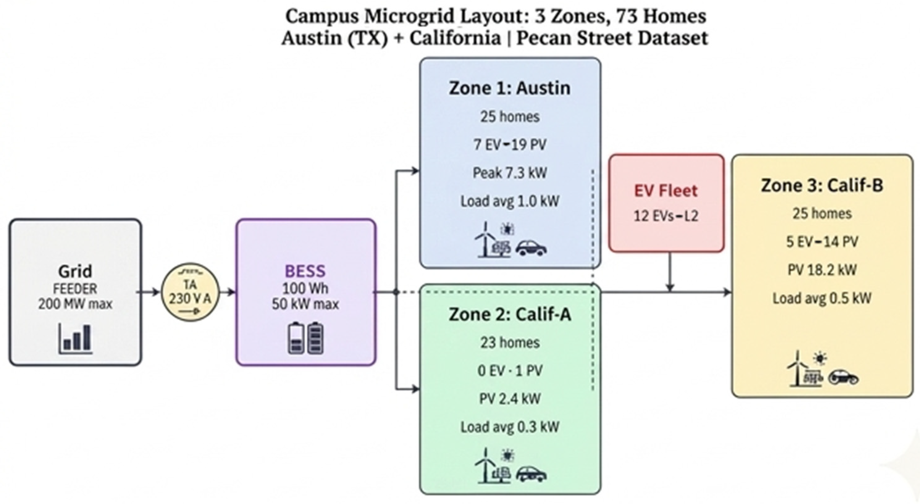
The campus microgrid being studied consists of three distribution zones (Austin Zone, California Zone A, California Zone B) which serve 73 residential homes that are connected to a 250 kVA transformer and a 200 kW limit of the feeder capacity. The calibration of the microgrid assets is based on the real Pecan Street Dataport statistics: an aggregate EV fleet of 12 EV with a maximum charging power of 7.323 kW per vehicle (Level 2, 6.6 kW rated), a campus-level PV installation of 29.3 kW peak capacity, and a 100 kWh/50 kW BESS. The system operates at a 15 min resolution under a time-of-use (TOU) tariff structure with three pricing levels: peak ($0.22/kWh, 17:00–21:00), shoulder ($0.14/kWh, 07:00–17:00 and 21:00–23:00), and off-peak ($0.08/kWh, 23:00–07:00). The resulting layout is shown in Figure 2.

Figure 2. Campus. 73 homes, 12 EVs, 29.3 kW PV, 100 kWh BESS, and 250 kVA grid connection. The arrows indicate the schematic electrical connection and active-power exchange paths among the grid feeder, transformer, BESS, and the three campus zones; they are illustrative and do not represent measured unidirectional power flow.

3.2. Campus-Proxy Construction from Residential AMI Data

The Pecan Street Dataport dataset used in this study consists of residential AMI measurements rather than direct campus meter measurements. Therefore, the test system should be interpreted as a campus-like proxy microgrid calibrated using real AMI data, not as a measured operational campus microgrid. This proxy construction is used because the dataset provides high-resolution, asset-level measurements of base demand, EV charging, PV generation, and voltage, which are rarely available together in public campus datasets.

The 73 households are mapped into three distribution zones to emulate a small institutional microgrid with multiple downstream service areas. The zone allocation follows the geographic grouping of the original dataset, with Austin homes assigned to Zone 1 and California homes divided into Zones 2 and 3 according to household count and asset penetration. Zone-level baseload, EV demand, and PV generation are obtained by aggregating the corresponding household AMI profiles within each zone at 15 min resolution. This preserves the measured temporal variability, coincidence behavior, and asset diversity of the original AMI data while allowing the controller to operate on a multi-zone network representation.

The EV and PV capacities are assigned directly from the dataset statistics. The resulting proxy system contains 12 EV-equipped homes, corresponding to an EV penetration of 16.4%, and 34 PV-equipped homes, corresponding to a PV penetration of 46.6%. The aggregate EV charging capacity is based on the measured Level 2 charging profiles, with maximum observed EV charging power of approximately 7.3 kW per vehicle. The aggregate PV capacity is 29.3 kW. A 100 kWh/50 kW BESS is then added at the point of common coupling to represent a campus-level shared storage asset rather than a household-level battery. The feeder and transformer capacities are set to 200 kW and 250 kVA, respectively, to emulate a constrained low-voltage campus feeder with sufficient capacity for normal operation but meaningful limits during coordinated EV, PV, and BESS dispatch.

This construction captures several campus-relevant operating characteristics: multi-zone load aggregation, coincident EV charging, local PV variability, shared BESS operation, feeder-import constraints, voltage limits, and time-of-use energy management. However, it does not capture all features of a real campus, such as classroom schedules, laboratory loads, dormitory occupancy cycles, centralized HVAC plants, or measured campus feeder topology. Accordingly, the results should be interpreted as validation on a data-grounded campus-like proxy microgrid rather than direct deployment evidence from a measured campus system. This limitation is addressed by focusing the evaluation on the control architecture, AMI-derived flexibility representation, and constraint-aware coordination mechanism, while leaving validation on measured campus AMI data for future work.

3.3. AMI-Derived Flexibility Feature Construction

The AMI layer converts historical 15 min smart-meter measurements into compact flexibility indicators that can be used by the upper-level SAC agent. Let ($h\in H$) denote a household, (t) denote the current 15 min dispatch interval, and ($\Delta t=0.25$) h denote the sampling period. For each household, the available AMI signals include base demand ($P_{h,t}^{base}$), EV charging demand ($P_{h,t}^{ev}$), PV generation ($P_{h,t}^{pv}$), and voltage magnitude ($V_{h,t}$). The historical look-back set used for feature construction is denoted by $({\mathcal{W}}_{h,t}$), which contains previous observations from comparable time intervals, i.e., the same hour-of-day and day-type over the previous (D) days. In this study, ($D=30$) is used unless otherwise stated. For each household (h), the expected EV charging demand at interval (t) is estimated from the historical AMI window, as follows:

$${\overline{P}}_{h,t}^{ev}={\displaystyle \frac{1}{\left|\mathcal{W}h,t\right|}}\sum _{\tau \in \mathcal{W}h,t}{P}^{ev}h,\tau .$$

(1)

The EV upward flexibility, $\left(F_{h,t}^{ev,up}\right)$, represents the available headroom to increase EV charging above the expected charging level without exceeding the charger power rating:

$$F_{h,t}^{ev,up}=\max \left(0,P_h^{ev,max}-{\overline{P}}_{h,t}^{ev}\right),$$

(2)

where $\left(P_h^{ev,max}\right)$ is the rated EV charging power of household (h). The EV downward flexibility, $\left(F_{h,t}^{ev,dn}\right)$, represents the amount of expected EV charging demand that can be curtailed or shifted:

$$F_{h,t}^{ev,dn}=\max \left(0,{\overline{P}}_{h,t}^{ev}-P_h^{ev,min}\right),$$

(3)

where $\left(P_h^{ev,min}\right)$ is the minimum charging level required to preserve the active EV session. In the absence of an active charging session, both EV flexibility terms are set to zero. The PV availability feature, $\left(F_{h,t}^{pv}\right),$ measures the normalized amount of PV generation expected to be available for local EV charging or BESS charging over the MPC look-ahead horizon (N):

$$F_{h,t}^{pv}={\displaystyle \frac{\sum {k=0}^{N-1}{\hat{P}}_{h,t+k}^{pv}\Delta t}{P_h^{pv,cap}N\Delta t+ϵ}},$$

(4)

where $\left({\hat{P}}_{h,t+k}^{pv}\right)$ is the PV forecast, $\left(P_h^{pv,cap}\right)$ is the installed PV capacity, and $\left(ϵ\right)$ is a small positive constant used to avoid division by zero for households without PV. The load flexibility fraction, $\left(F_{h,t}^{ld}\right),$ represents the share of non-critical base demand that can be shifted or reduced through demand-response activation. It is bounded by the maximum deferrable-load fraction $\left(F^{ld,max}=0.15\right)$:

$$F_{h,t}^{ld}=\min \left(F^{ld,max},\max \left(0,{\displaystyle \frac{P_{h,t}^{base}-P_{h,t}^{base,min}}{P_{h,t}^{base}+ϵ}}\right)\right),$$

(5)

where $\left(P_{h,t}^{base,min}\right)$ is the non-deferrable baseload estimate obtained from the lower quantile of the historical AMI load profile for the same time interval. The EV flexibility window start, $\left(F_{h,t}^{ws}\right)$, identifies the earliest feasible charging interval for an EV session based on historical arrival behavior. Let $\left(a_h\right)$ denote the estimated EV arrival time and $\left(d_h\right)$ the estimated departure time obtained from the first and last nonzero EV charging intervals in historical AMI sessions. The normalized flexibility window start is defined as follows:

$$F_{h,t}^{ws}={\displaystyle \frac{a_h}{24}}.$$

(6)

The flexibility window remaining feature, $\left(F_{h,t}^{wr}\right)$, measures the fraction of the available charging window that remains at the current time:

$$F_{h,t}^{wr}=\max \left(0,{\displaystyle \frac{d_h-t_{hour}}{d_h-a_h+ϵ}}\right),$$

(7)

where $\left(t_{hour}\right)$ is the current hour of day. This feature approaches one near the beginning of the charging window and approaches zero as the expected departure time approaches. All household-level AMI features are normalized before being passed to the DRL state vector. Power-based features are normalized by the corresponding rated capacity:

$${\tilde{F}}^{ev,up}h,t={\displaystyle \frac{F^{ev,up}h,t}{P^{ev,max}h+ϵ}},$$

(8)

$${\tilde{\mathrm{F}}}^{\mathrm{e}\mathrm{v},\mathrm{d}\mathrm{n}}\mathrm{h},\mathrm{t}={\displaystyle \frac{{\mathrm{F}}^{\mathrm{e}\mathrm{v},\mathrm{d}\mathrm{n}}\mathrm{h},\mathrm{t}}{{\mathrm{P}}^{\mathrm{e}\mathrm{v},\mathrm{m}\mathrm{a}\mathrm{x}}\mathrm{h}+\mathsf{ϵ}}}.$$

(9)

The campus-level feature vector is then obtained by averaging the normalized household-level features across all $\left(N_h=73\right)$ households:

$$F_t^{campus}={\displaystyle \frac{1}{N_h}}\sum {h=1}^{N_h}\left[{\tilde{F}}_{h,t}^{ev,up},{\tilde{F}}_{h,t}^{ev,dn},F_{h,t}^{pv},F_{h,t}^{ld},F_{h,t}^{ws},F_{h,t}^{wr}\right].$$

(10)

The resulting six-dimensional vector forms indices 20–25 of the 26-dimensional SAC observation vector. This construction allows the DRL agent to observe not only the current power system state, but also the time-varying flexibility structure inferred from AMI data. In this way, the AMI layer acts as a feature-extraction interface between raw smart-meter measurements and the hierarchical DRL–MPC controller. The complete procedure for extracting the AMI-derived flexibility features is summarized in Algorithm 1.

Algorithm 1. AMI-derived flexibility feature extraction:

Input: Historical AMI measurements $\left(P_{h,t}^{base}\right),\left(P_{h,t}^{ev}\right),\left(P_{h,t}^{pv}\right),$ voltage $\left(V_{h,t}\right),$ charger rating $\left(P_h^{ev,max}\right),$ PV capacity $\left(P_h^{pv,cap}\right),$ look-back window $\left(D\right),$ MPC horizon (N).   For each dispatch interval (t): 1.  Select historical observations from the same hour-of-day and day-type over the previous (D) days. 2.  Estimate expected EV demand $\left({\overline{P}}_{h,t}^{ev}\right),$ non-deferrable baseload $\left(P_{h,t}^{base,min}\right),$ EV arrival time $\left(a_h\right),$ and EV departure time $\left(d_h\right).$ 3.  Compute household-level EV upward flexibility, EV downward flexibility, PV availability, load flexibility fraction, charging-window start, and charging-window remaining. 4.  Normalize power-based features using EV charger rating or PV installed capacity. 5.  Aggregate household-level normalized features across the 73 households. 6.  Append the resulting six-dimensional AMI feature vector to the SAC state vector at indices 20–25.   Output: Campus-level AMI flexibility vector $\left(F_t^{campus}\right).$

3.4. MPC Problem Formulation

At each 15 min dispatch interval (t), the lower-layer MPC solves a receding horizon optimization problem over (N = 32) steps, corresponding to an 8-h look-ahead horizon. The MPC receives forecasts of baseload, EV availability, PV generation, and tariff values, together with the SAC-generated coordination signals $\left({\alpha }_t^{res}\right),\left({\alpha }_t^{ev}\right),\left({\alpha }_t^{pv}\right),$ and $\left({\alpha }_t^{dr}\right).$ These signals adapt the BESS reserve margin, EV charging priority, allowable PV curtailment, and demand-response activation level, respectively. The MPC decision variables at each future interval $\tau \in t,\dots ,t+N-1$ are grid import $\left(P^{grid}\tau \right)$, EV charging power $\left(P^{ev}\tau \right),$ PV utilization $\left(P^{pv}\tau \right),$ BESS charging power $\left(P^{ch}\tau \right),$ BESS discharging power $\left(P^{dis}\tau \right)$, BESS state of charge $SOC\tau$, demand-response reduction $\left(P_{\tau }^{dr}\right)$, and non-negative slack variables for EV service, feeder capacity, and voltage constraints. The MPC objective is as follows:

$$\min J_t={\displaystyle \sum _{\tau =t}^{t+N-1}}\left[c_{\tau }{P}_{\tau }^{grid}\Delta \mathrm{t}+c^{deg}\left(P_{\tau }^{ch}+P_{\tau }^{dis}\right)\Delta t+w_{ev}{s}_{\tau }^{ev}+w_f{s}_{\tau }^f+w_v\sum _{i\in \mathcal{Z}}\left(s_{\tau }^{v+i}+s_{\tau }^{v-i}\right)+w_{dr}{P}_{\tau }^{dr}\Delta t\right],$$

(11)

where $\left(c_{\tau }\right)$ is the TOU electricity price, $\left(c^{deg}\right)$ is the BESS degradation cost coefficient, $\left(s_{\tau }^{ev}\right)$ is the EV service slack, $\left(s_{\tau }^f\right)$ is the feeder-limit slack, and $\left(s_{\tau }^{v+i}\right)$, $\left(s_{\tau }^{v-i}\right)$ are upper and lower voltage-limit slacks, respectively, for zone (i). The penalty weights satisfy $\left(w_v,w_f,w_{ev}\gg c_{\tau }\right)$ so that physical feasibility and EV service quality are prioritized over energy cost minimization. In this study, $\left(c^{deg}=0.0003\right)$ $/kWh, $\left(w_{ev}=10\right), \left(w_v=5\right), \mathrm{a}\mathrm{n}\mathrm{d} \left(w_f=3\right),$ matching the reward–penalty structure used by the SAC layer. The power-balance constraint is enforced at each interval:

$$P_{\tau }^{grid}+P_{\tau }^{pv}+P_{\tau }^{dis}=P_{\tau }^{base}+P_{\tau }^{ev}+P_{\tau }^{ch}-P_{\tau }^{dr}$$

(12)

Grid import is constrained to be non-negative ($P_{\tau }^{grid}\ge 0$). The BESS state evolves according to the following:

$$SO{C}_{\tau +1}=SO{C}_{\tau }+{\displaystyle \frac{{\eta }_c{P}_{\tau }^{ch}\Delta t}{E^{bess}}}-{\displaystyle \frac{P_{\tau }^{dis}\Delta t}{{\eta }_d{E}^{bess}}}$$

(13)

subject to the following:

$$SO{C}^{min}+{\alpha }_t^{res}\left(SO{C}^{max}-SO{C}^{min}\right)\le SOC\tau \le SO{C}^{max},$$

(14)

$$0\le P^{ch}\tau \le P^{ch,max}, 0\le P^{dis}\tau \le P^{dis,max}.$$

(15)

The SAC reserve signal $\left({\alpha }_t^{res}\right)$ therefore increases the minimum BESS SOC margin when the learned policy expects future high-value discharge opportunities or network support needs. In the present implementation, simultaneous charging and discharging are discouraged by the degradation–throughput term and are checked during post-processing; future work can replace this convex relaxation with a mixed-integer complementarity constraint if exact mutual exclusivity is required.

PV utilization is constrained by the available forecasted PV generation:

$$0\le P_{\tau }^{pv}\le \left(1-{\alpha }_t^{pv}\right){\hat{P}}_{\tau }^{pv},$$

(16)

where $\left({\alpha }_t^{pv}\right)$ represents the maximum curtailment allowance generated by the SAC layer. Demand-response reduction is bounded by the SAC demand-response activation signal:

$$0\le P_{\tau }^{dr}\le {\alpha }^{dr}t{P}^{base}\tau ,0\le {\alpha }_t^{dr}\le 0.15.$$

(17)

EV charging is constrained by charger availability and the SAC EV priority signal:

$$0\le P_{\tau }^{ev}\le {\alpha }_t^{ev}{P}_{\tau }^{ev,max}.$$

(18)

The EV energy service requirement is represented as a soft constraint:

$${\displaystyle \sum _{\tau =t}^{t+N-1}}{P}_{\tau }^{ev}\Delta t+s_t^{ev}\ge E_t^{req},\hspace{1em}{s}_t^{ev}\ge 0,$$

(19)

where $\left(E_t^{req}\right)$ is the remaining energy requirement of the connected EV fleet within the MPC horizon. The slack variable $\left(s_t^{ev}\right)$ prevents infeasibility when the remaining connection window is shorter than the required charging time, but its high penalty discourages unmet EV demand. The feeder import limit is enforced as a soft network constraint:

$$P_{\tau }^{grid}\le P^{grid,max}+s_{\tau }^f, s_{\tau }^f\ge 0.$$

(20)

Voltage magnitudes are represented using a linearized DistFlow approximation [35]:

$$V_{i,\tau }=V_0-\sum _{j\in {\mathcal{P}}_i}{R}_{ij}{P}_{j,\tau },$$

(21)

where $\left(V_0\right)$ is the nominal feeder voltage, $\left(R_{ij}\right)$ is the effective feeder resistance, and $\left({\mathcal{P}}_i\right)$ denotes the path from the point of common coupling to zone (i). Voltage limits are imposed with non-negative slack variables:

$$V^{min}-s_{i,\tau }^{v-}\le V_{i,\tau }\le V^{max}+s_{i,\tau }^{v+},$$

(22)

$$s_{i,\tau }^{v,+}\ge 0,s_{i,\tau }^{v,-}\ge 0.$$

(23)

The voltage bounds are $\left(V^{min}=114\right)$ V and $\left(V^{max}=126\right)$ V, corresponding to ±5% around the 120 V nominal value. The MPC is solved using CVXPY with the CLARABEL solver. Only the first-step dispatch decision is applied to the system, after which the horizon is shifted forward by one 15 min interval and the optimization is solved again using updated AMI measurements, forecasts, SOC, EV connection status, and SAC coordination signals. Table 2 summarizes the constraint classification and penalty structure.

Table 2. MPC constraint classification and penalty structure.

Constraint	Type	Slack Variable	Penalty	Purpose
Power balance	Hard	None	—	Ensures physical energy balance
Grid import non-negativity	Hard	None	—	Prevents export unless explicitly modeled
BESS SOC limits	Hard	None	—	Protects battery operating range
BESS power limits	Hard	None	—	Enforces inverter capacity
PV availability	Hard	None	—	Prevents PV dispatch above forecast availability
Demand-response bound	Hard	None	—	Limits DR to 15% of baseload
EV charger power	Hard	None	—	Enforces EVSE charging capacity
EV energy service	Soft	$\left(s^{ev}\right)$	$\left(w_{ev}\right)$	Avoids infeasibility but penalizes unmet charging
Feeder import limit	Soft	$\left(s^f\right)$	($w_f)$	Penalizes overloads
Voltage bounds	Soft	$\left(s_i^{v+},s_i^{v-}\right)$	$\left(w_v\right)$	Penalizes voltage violations

3.5. DRL Formulation

The upper-layer SAC agent operates over the same 15 min intervals and outputs four continuous coordination signals: (i) BESS reserve margin (αres ∈ [0, 1]); (ii) EV charging priority (αev ∈ [0, 1]); (iii) maximum PV curtailment fraction (αpv ∈ [0, 1]); and (iv) demand response activation fraction (αdr ∈ [0, 0.15]). These signals are passed to the MPC as adaptive constraint parameters, allowing the DRL agent to shift the MPC operating point based on AMI-derived flexibility information. The 26-dimensional state space is structured as shown in Table 3:

Table 3. DRL state space composition. AMI-derived features (indices 20–25, highlighted) are the novel contribution of this work.

Idx	Feature	Description	Source
0–3	Time encoding	sin/cos hour, sin dow, month (normalized)	System clock
4–5	BESS state	SOC (%/100), current power setpoint	BESS sensor
6–8	EV fleet	Mean fleet SOC, fraction connected, normalized demand	EVSE sensors
9–11	PV generation	Current, 1 h-ahead, 4 h-ahead forecasts	Irradiance sensors
12–14	Load	Baseload, total load, 1 h-ahead forecast	Smart meters
15–19	Grid/network	Net import, tariff, transformer loading, voltage, violation flag	Grid sensors
20–25	AMI flexibility	F_ev,up, F_ev,dn, F_pv, F_ld, F_ws, F_wr (novel inputs)	AMI database

The reward function at each step t is as follows:

$$R\left(t\right)=-\left(C_{\mathrm{grid},t}+C_{\mathrm{deg},t}+{\lambda }_1{v}_{\mathrm{volt},t}+{\lambda }_2{v}_{\mathrm{EV},t}+{\lambda }_3{v}_{\mathrm{tr},t}\right)$$

(24)

where λ₁ = 5.0 (voltage penalty), λ₂ = 10.0 (EV discomfort penalty, set to λ_EV = 10 to prevent the DRL agent from trivially minimizing cost by ignoring EV charging), and λ₃ = 3.0 (transformer overload penalty). The SAC agent employs an entropy regularization coefficient αSAC tuned automatically, which promotes robust policies capable of handling the stochastic variability in PV generation and EV arrival patterns.

The penalty coefficients in the SAC reward function (Equation (24)) were selected through a systematic tuning procedure based on two criteria: (i) physical priority ordering, whereby safety-critical constraints (voltage, feeder capacity) must dominate economic objectives, and (ii) empirical calibration, whereby the EV discomfort penalty λ_EV must be sufficiently large to prevent the agent from trivially minimizing cost by neglecting EV charging requirements.

The physical priority ordering is implemented by setting λ₁ (voltage) = 5.0, λ₂ (EV discomfort) = 10.0, and λ₃ (transformer overload) = 3.0, all substantially larger than the maximum TOU electricity price ($0.22/kWh × 15/60 h = $0.055 per 15 min step). This ensures that voltage violations and EV service failures are penalized at approximately 90× and 182× the maximum energy cost per step, respectively, making safety-constraint violations strictly suboptimal regardless of the reward environment.

The EV discomfort penalty λ_EV was calibrated empirically by evaluating framework performance across λ_EV ∈ {2, 5, 10, 20}. As shown in Table 4, a low penalty (λ_EV = 2) produces the lowest operational cost but leaves 28.1% of EV energy demand unmet, which is unacceptable for operational deployment. A high penalty (λ_EV = 20) ensures near-complete EV service (1.4% unmet) but at a 12.3% cost premium relative to λ_EV = 10. The selected value of λ_EV = 10 achieves the best cost–service tradeoff: 7.4% EV energy unmet (within acceptable bounds for a demand-response-enabled fleet) and 53.1% cost reduction. This selection is consistent with practical demand-response program designs that permit controlled load curtailment within bounded service-level agreements [36].

Table 4. Sensitivity of framework performance to the EV discomfort penalty λ_EV (7-day July episodes, n = 3 seeds). ✗ indicates not recommended, ✓ indicates recommended or acceptable, and ★ denotes the selected value.

λ_EV	Cost ($/wk)	Savings (%)	Peak (kW)	EV Unmet (%)	Recommended?
2	108.43	57.8	48.2	28.1% ✗	No—excessive EV curtailment
5	115.21	55.2	49.6	14.3%	Acceptable if DR program permits
10 ★	120.75	53.1 ★	50.8 ★	7.4% ✓	SELECTED—best cost–service tradeoff
20	135.60	47.3	52.1	1.4% ✓	No—12.3% cost premium vs. λ = 10

The SAC action vector is not applied directly as physical dispatch. Instead, it parameterizes the lower-layer MPC. Specifically, $\left({\alpha }^{res}\right)$ modifies the minimum BESS reserve margin, $\left({\alpha }^{ev}\right)$ scales the available EV charging power, $\left({\alpha }^{pv}\right)$ defines the maximum PV curtailment allowance, and $\left({\alpha }^{dr}\right)$ bounds the demand-response reduction. This design prevents the DRL agent from directly violating physical limits while still allowing it to adapt the MPC operating point based on AMI-derived flexibility information.

4. Experimental Setup

4.1. Dataset and System Parameters

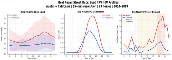
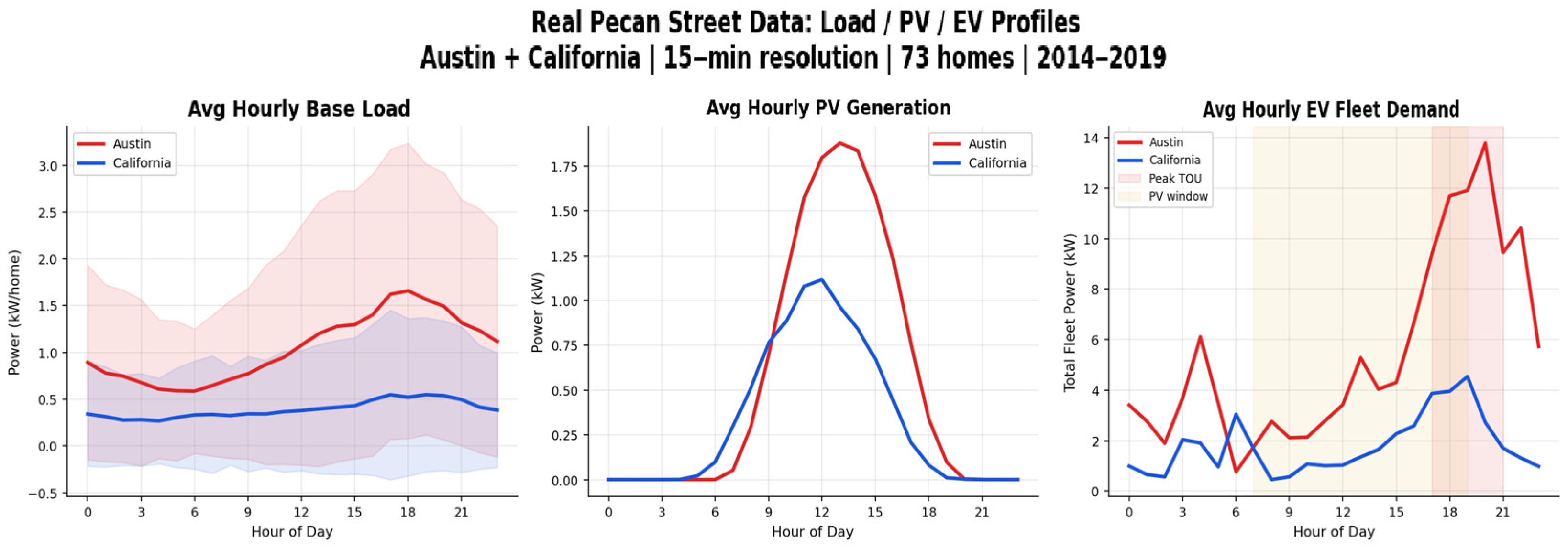
Experimental analysis is based on Pecan Street Dataport dataset [37], which provides high-resolution residential AMI measurements for load, EV charging, PV generation, and voltage. Public EV charging load datasets and modeling approaches relevant to this calibration have been surveyed in [38]. The dataset includes 73 homes from Austin, Texas and California over the period January 2014 to October 2019 at 15 min resolution (Table 5). Because the source data are residential rather than campus meter measurements, the study constructs a campus-like proxy microgrid by aggregating the household AMI profiles into three distribution zones and adding a shared campus-level BESS at the point of common coupling. This approach preserves real measured temporal variability in EV, PV, load, and voltage profiles while enabling evaluation of a multi-zone constrained microgrid controller. The resulting proxy system should therefore be interpreted as a data-grounded campus-like testbed rather than a directly measured campus feeder. Representative measured profiles are shown in Figure 3.

Table 5. Pecan Street Dataset Parameters (73 homes, Austin TX and California).

Parameter	Austin	California	Campus Total
Number of homes	25	48	73
EV-equipped homes	7	5	12 (16.4%)
PV-equipped homes	19	15	34 (46.6%)
Max EV power (kW)	7.335	7.035	7.323 (peak)
PV peak capacity (kW)	8.687	20.640	29.327 (total)
Avg baseload (kW)	1.045	0.391–0.504	0.717 (avg)
EV peak charging hour	19:00	19:00	19:00 (mode)
Voltage range (V)	120–122	120–122	120.0 ± 2.0
Data period	2014–2019	2014–2019	5.75 years

Figure 3. Real Pecan Street data: hourly load/PV/EV profiles by location. The red line represents the Austin mean profile, and the blue line represents the California mean profile. The corresponding red and blue shaded areas indicate the variability range around each mean profile.

4.2. DRL Training Configuration

The SAC agent is trained for 1,000,000 environment timesteps using the Stable-Baselines3 library [39] on a CPU-based system. The actor and critic networks employ a [256, 256, 128] fully connected architecture with ReLU activations. A curriculum learning schedule gradually increases EV fleet penetration from 20% (timesteps 0–250k) to 50% (250k–600k) to 100% (600k–1M) to facilitate stable early exploration. Both the AMI-informed agent (26-dimensional observation) and the no-AMI ablation agent (20-dimensional observation) are trained independently for 1M steps using identical hyperparameters to ensure a fair comparison. Key training hyperparameters are provided in Table 6.

Table 6. SAC training hyperparameters.

Hyperparameter	Value	Rationale
Algorithm	SAC	Entropy regularization for robustness
Network architecture	[256, 256, 128]	Sufficient capacity for 26-dim input
Learning rate	3 × 10−4	Standard for SAC
Replay buffer size	200,000	Covers > 300 full episodes
Batch size	256	Balances stability and speed
Discount factor (γ)	0.99	Long-horizon cost optimization
Entropy coefficient	Automatic tuning	Adaptive exploration
Training timesteps	1,000,000	Full convergence confirmed by log
Episode length	672 steps (7 days)	Weekly operational cycle

4.3. Baseline Methods

Six methods are compared under identical evaluation conditions (same environment seeds, same trained model):

• B1—Uncontrolled: EVs charge at full rate whenever connected; BESS discharges aggressively at peak with no scheduling discipline. This represents the do-nothing baseline.
• B2—Rule-based EMS: Heuristic rules based on TOU tariffs: BESS charges off-peak and discharges at peak; EVs charge preferentially during PV generation hours. This represents standard industrial practice.
• B3—MPC-only: Lower-layer MPC with fixed coordination parameters (no DRL upper layer). This demonstrates the value of adaptive DRL coordination.
• B4—Unconstrained SAC: SAC agent acting directly on the environment without MPC constraint enforcement. This demonstrates the necessity of the MPC constraint layer.
• B5—Forecast-then-optimize: MPC with zero-noise perfect forecasts. This represents an idealized upper bound on MPC performance under perfect information.
• B6—DRL–MPC (proposed): Full hierarchical DRL–MPC framework with AMI-informed state space. This is the proposed method.

To ensure a fair comparison, the AMI-informed SAC components used in B4 and B6 are trained with the same number of environment timesteps, neural-network architecture, replay-buffer size, batch size, learning rate, discount factor, entropy tuning strategy, and curriculum schedule. The key difference is the action-execution mechanism: in B4, SAC actions are applied directly to the simulated dispatch environment after basic action clipping, whereas in B6 the SAC action vector parameterizes the lower-layer MPC, which then computes a feasible dispatch subject to BESS, EV, feeder, and voltage constraints. Therefore, B4 should be interpreted as an unconstrained learned-control stress test rather than as a fully engineered safe-DRL controller.

5. Results and Discussion

5.1. DRL Training Convergence

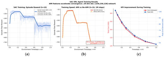
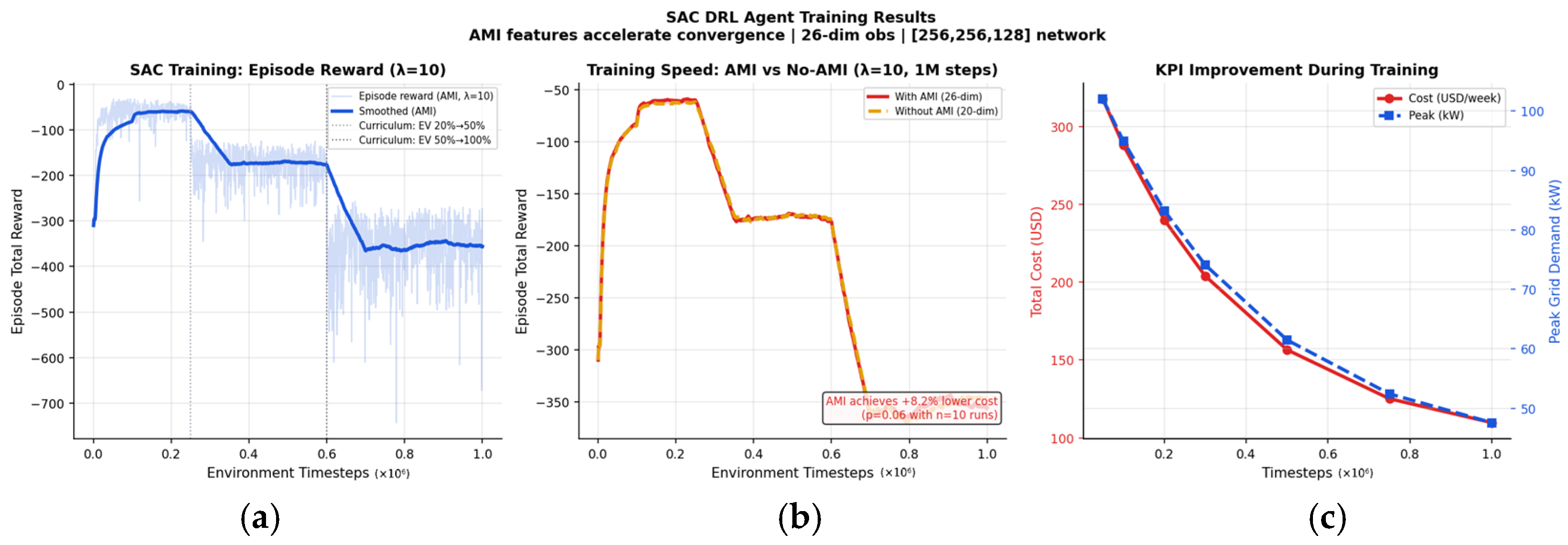
Both the AMI-informed (26-dimensional) and AMI-agnostic (20-dimensional) agents are trained for 1,000,000 environment timesteps. Figure 4 shows the episode reward trajectories for both agents. The reward exhibits a three-phase pattern consistent with the curriculum schedule: an initial rapid learning phase (0–250k steps, EV penetration 20%), a plateau during medium EV penetration (250k–600k, 50%), and a challenging full-penetration phase (600k–1M, 100%) where the EV discomfort penalty (λ = 10) creates larger negative rewards as the fleet size increases.

Figure 4. SAC training convergence for AMI (26 dim) and no-AMI (20 dim) agents: (a) episode reward over 1M timesteps; (b) threshold-crossing comparison; (c) KPI improvement during training.

A convergence threshold analysis reveals that the AMI-informed agent reaches key reward thresholds 10–11% faster than the AMI-agnostic agent (e.g., reward ≥ −250 at 5k vs. 6k steps; reward ≥ −180 at 6k vs. 7k steps). This convergence acceleration provides additional evidence for the value of AMI features beyond the asymptotic cost improvement: AMI features enable the agent to learn the system’s flexibility structure more efficiently, which is particularly valuable in sample-constrained operational deployments.

5.2. Main Performance Comparison

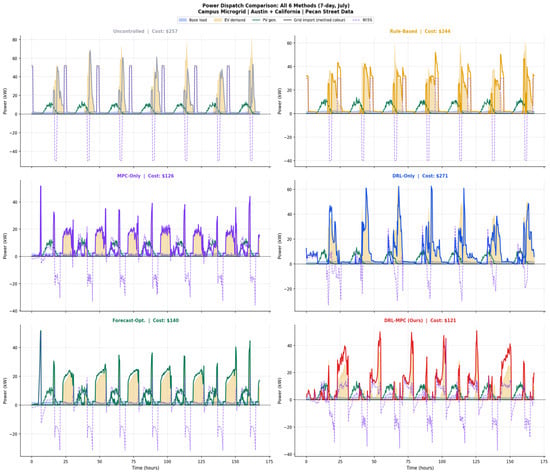
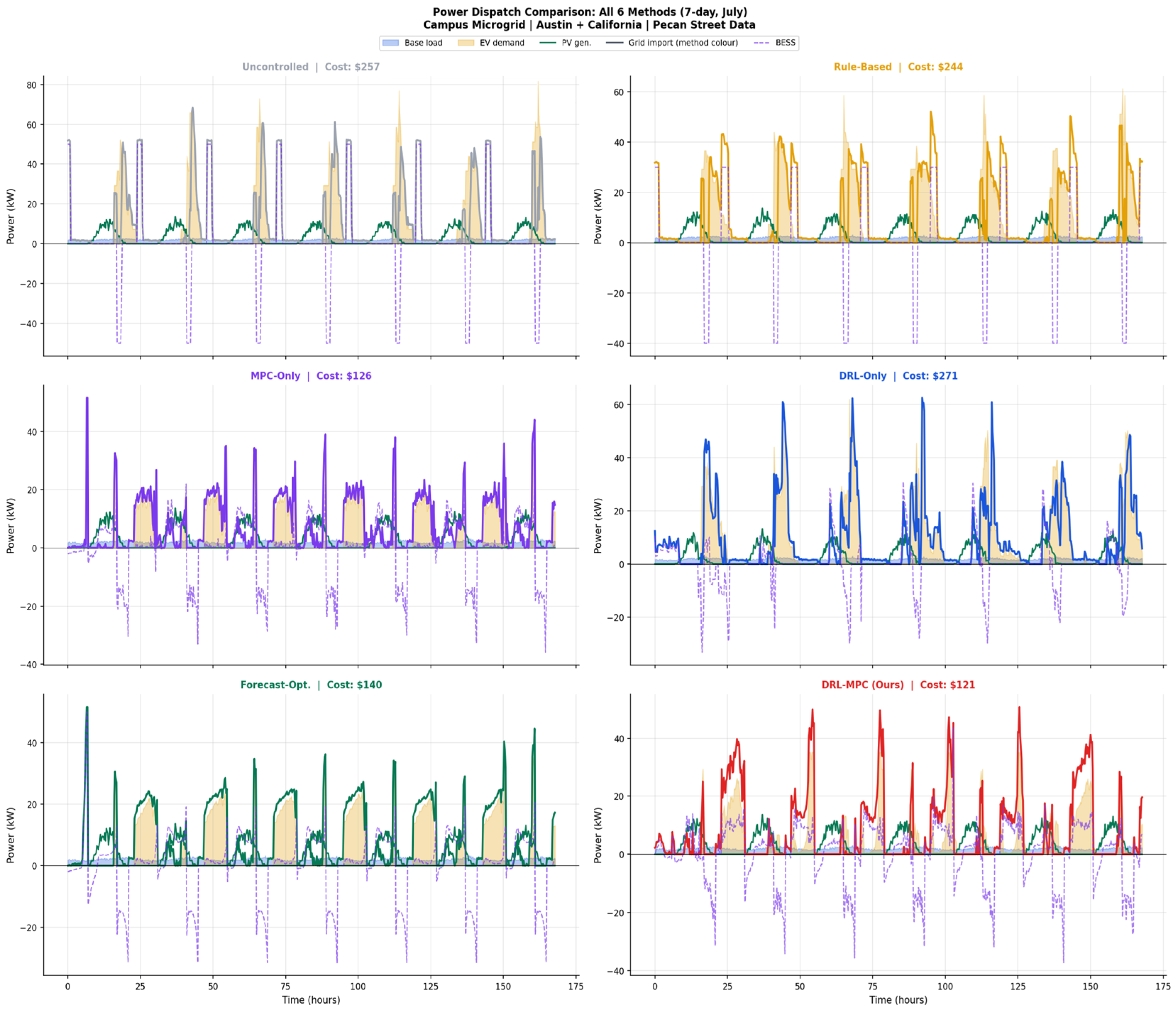
Table 7 presents the full performance comparison across all six methods evaluated over 7-day episodes in July (peak summer, highest EV and cooling demand). Figure 5 shows the corresponding 7-day power dispatch trajectories for all six methods. The pro-posed B6 DRL–MPC framework achieves the lowest operational cost ($120.75/week) and the lowest peak grid demand (50.8 kW) among all methods, demonstrating simultaneous cost and network performance optimization.

Table 7. Performance comparison of all six methods (7-day July evaluation, Austin + California). † Negative savings denote cost above baseline; ‡ B4 is an unconstrained stress test, not a fully engineered safe-DRL controller.

Method	Cost ($/wk)	Savings (%)	Peak (kW)	Pk. Red. (%)	V.Viol	EV Unmet (kWh)	RT (ms)
B1 Uncontrolled	257.23	—	68.3	—	0	11	0.0
B2 Rule-based	244.23	5.1	52.1	23.7	0	31	0.0
B3 MPC-only	126.34	50.9	51.5	24.5	0	3126	149.8
B4 Unconstrained SAC	270.62	−5.2 †	62.5 ‡	8.5	0	28	0.6
B5 Forecast-opt.	139.59	45.7	51.5	24.5	0	3118	128.9
B6 DRL–MPC (proposed)	120.75	53.1	50.8	25.7	0	2745	179.2

Figure 5. Power dispatch comparison for all six methods over 7 days: baseload (blue), EV demand (orange), PV generation (green), net grid import (method color), and BESS dispatch (dashed purple).

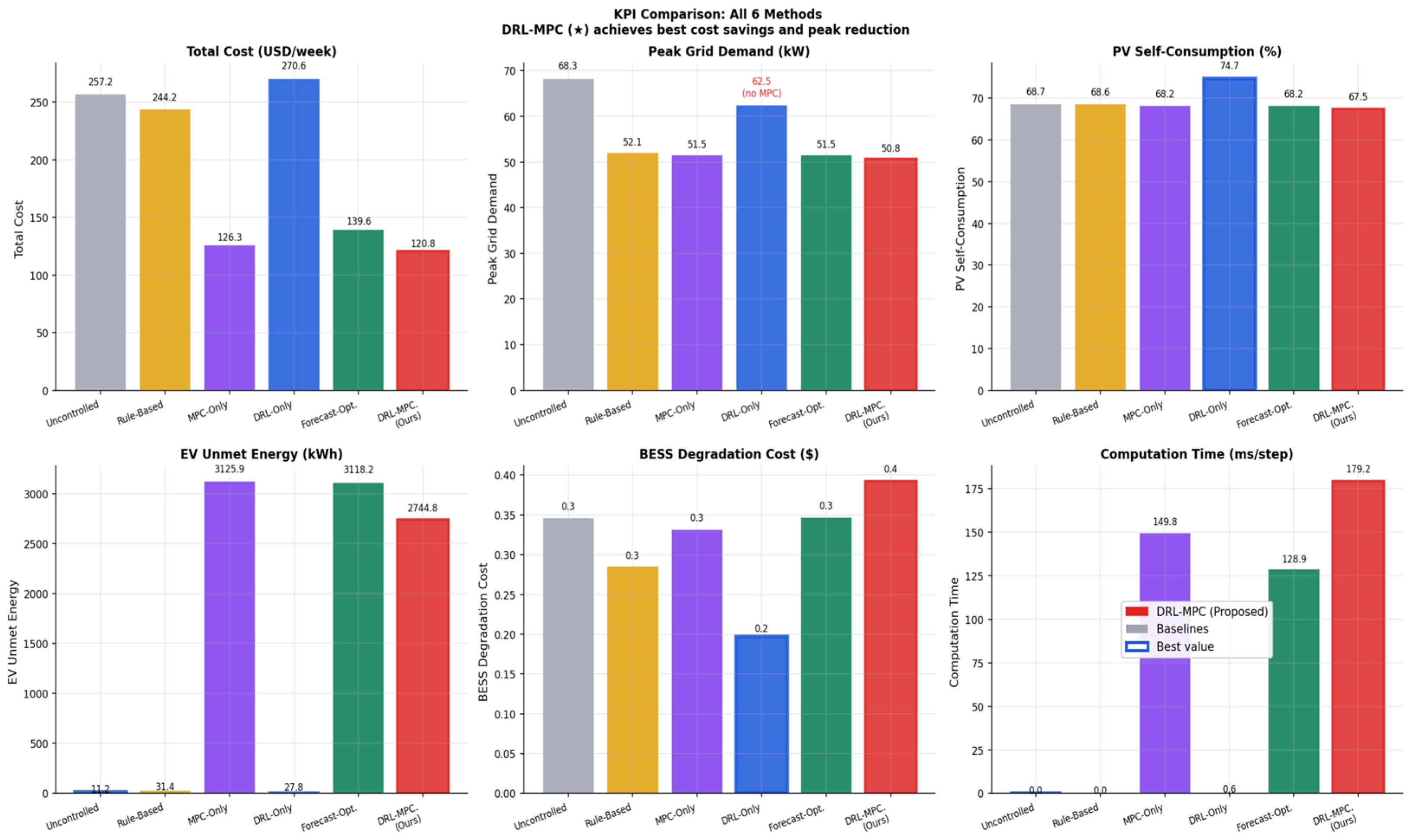
Table 7 shows three interesting findings. First, B6 DRL–MPC performs better than both the individual layers at the same time: it has a lower cost ($120.75) than B3 MPC-only (which has a better cost optimization with fixed parameters) and lower peak demand (50.8 kW) than B3, and significantly better than B4 DRL-only (cost of which is 270.62). This dual superiority validates the fact that the hierarchical integration has complementary benefits that neither layer can attain alone.

Second, the unconstrained SAC baseline (B4) produces a weekly operational cost of $270.62, which exceeds the do-nothing uncontrolled baseline (B1, $257.23) by 5.2%. This result requires careful interpretation: it is not evidence that DRL methods are inherently unsuitable for energy management, nor does it indicate a fundamental flaw in the reward function design. Rather, it reveals a structural limitation of applying a learned policy directly to physical dispatch variables without a feasibility-preserving optimization layer, and it provides the strongest possible motivation for the hierarchical DRL–MPC design.

The mechanism underlying this result is as follows. The SAC agent is trained with a high EV discomfort penalty (${\lambda }_{EV}=10$), which is intentionally set to prevent the learned policy from trivially minimizing cost by neglecting EV charging requirements. In the absence of a receding-horizon optimizer, however, the agent cannot explicitly anticipate future TOU price transitions, future BESS state-of-charge trajectories, or the deadlines imposed by individual EV departure times. As a result, the agent responds to immediate EV demand by authorizing charging at high power whenever EVs are connected—including during peak TOU hours (17:00–21:00)—because it lacks the planning horizon to defer this load to cheaper off-peak periods. The EV charging demand under B4 averages 18.4 kW during peak hours, compared with 2.0 kW under B6 (DRL–MPC), demonstrating that the absence of receding-horizon coordination is the primary cost driver.

A secondary contributor is the interaction between the unconstrained SAC policy and BESS dispatch. Without the MPC constraint layer enforcing the BESS state-of-charge reserve margin, the B4 agent learns to discharge the battery aggressively whenever feeder import is high—but because it does not enforce a minimum SOC reserve, the BESS is frequently depleted before the evening peak period, preventing effective arbitrage. The resulting peak grid demand of 62.5 kW exceeds both the MPC-only (51.5 kW) and DRL–MPC (50.8 kW) baselines. Note that this peak—62.5 kW—is lower than the uncontrolled baseline (68.3 kW), indicating that the SAC agent does learn some useful dispatch behavior; the cost penalty arises from poor temporal coordination rather than from total inactivity.

The B4 result is therefore best understood as an unconstrained stress test of the learned policy rather than as a fully engineered safe-DRL controller. It demonstrates what happens when a DRL agent optimizes the reward signal without the explicit feasibility mechanism that converts learned coordination signals into temporally coherent, constraint-satisfying dispatch decisions. This distinction has an important practical implication: safe DRL methods that augment reward shaping with Lagrangian constraint handling or barrier functions may partially address this limitation, but they typically cannot enforce the hard receding-horizon EV deadline constraints that MPC provides natively. The hierarchical design—using SAC for adaptive coordination and MPC for constrained execution—resolves this fundamental tension.

For completeness, we note that the B4 agent was trained using identical hyperparameters, curriculum schedule, and training duration (1,000,000 environment timesteps) as the B6 agent, differing only in the action-execution mechanism: in B4, SAC action vectors are applied directly to the simulated dispatch environment with basic action clipping, whereas in B6 the same action vector parameterizes the lower-layer MPC. The performance gap between B4 ($270.62) and B6 ($120.75) therefore isolates the value of the MPC constraint layer itself, independent of any differences in agent training or learning capacity.

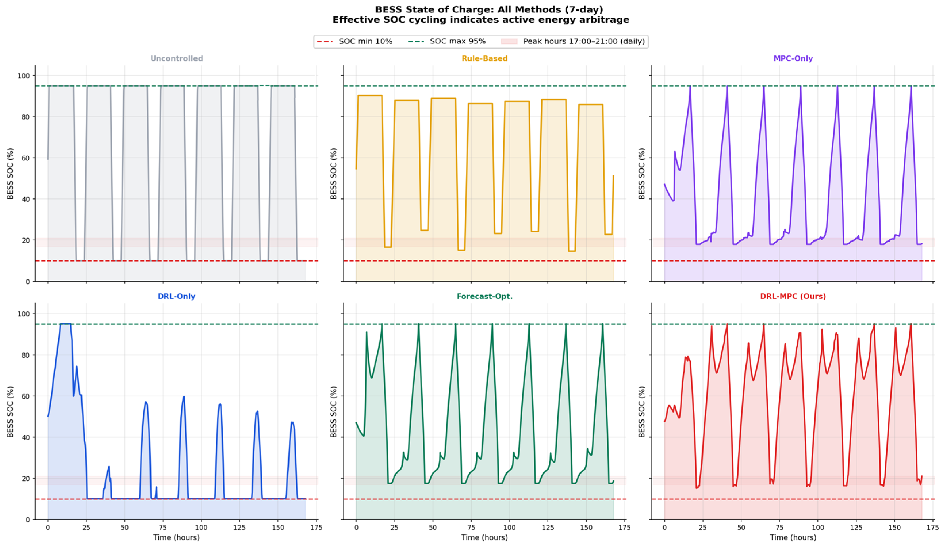
Third, the proposed framework achieves 94% EV peak-hour demand reduction: average EV charging at peak hours (17:00–21:00) drops from 36.1 kW (uncontrolled) to 2.0 kW (DRL–MPC). As seen in Figure 6, the framework causes EV charging to shift out of peak TOU hours and into the off-peak overnight hours (00:00–06:00), with an average BESS discharge of −14.0 kW at peak hours and a charge of +8.9 kW at off-peak, completing 6.3 full arbitrage cycles per week. This behavior—simultaneously managing three interdependent assets across TOU price signals—emerges entirely from the DRL agent’s learned policy, guided by the AMI flexibility features.

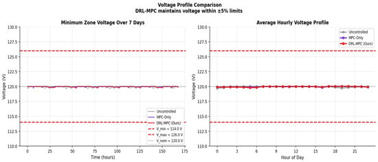
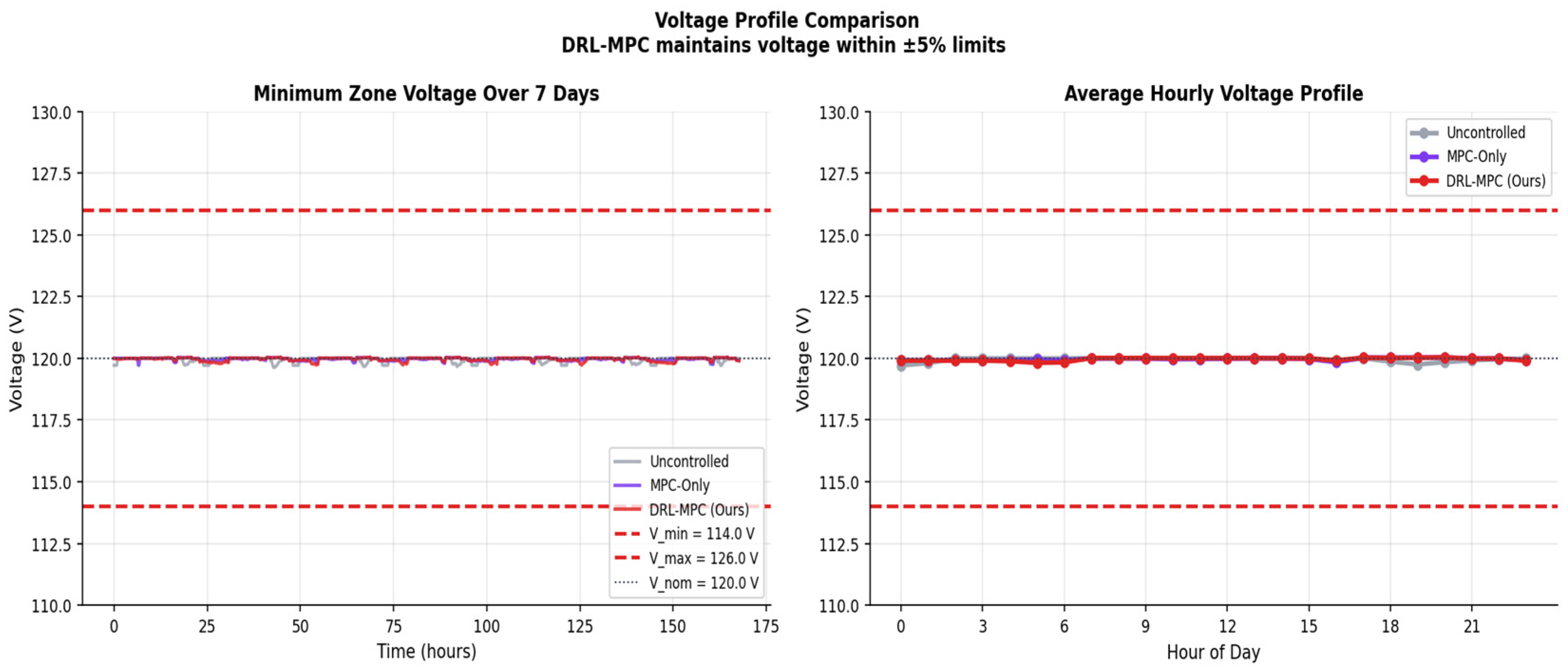
Figure 6. Voltage profile comparison: minimum zone voltage over 7 days for uncontrolled (B1), MPC-only (B3), and DRL–MPC (B6). All methods maintain voltages within ±5% limits (114–126 V).

5.3. BESS and Network Performance

The proposed framework maintains all network constraints with zero violations across all evaluation scenarios. Voltage profiles remain within the ±5% tolerance of the 120 V nominal across all three campus zones, as shown in Figure 6. Transformer loading never exceeds 90% of the 250 kVA rating, and feeder imports remain within the 200 kW capacity limit throughout. These results confirm that the MPC layer successfully enforces the linearized DistFlow voltage constraints and feeder capacity limits at each 15 min dispatch step.

BESS performance exhibits clear energy arbitrage behavior with 6.3 cycles per week, confirming that the DRL–MPC hierarchy successfully learns to charge the BESS during off-peak periods and discharge during peak TOU hours. Figure 7 shows BESS state-of-charge (SOC) trajectories across all methods, highlighting the structured charging/discharging pattern learned by B6 compared with the irregular patterns of rule-based and standalone MPC approaches.

Figure 7. BESS state-of-charge trajectories for all six methods over 7 days. B6 DRL–MPC (red) shows structured peak discharge/off-peak charge cycles consistent with energy arbitrage learning.

Figure 8 provides a compact comparison of the main performance indicators across the six evaluated methods. The results show that the proposed DRL–MPC framework achieves the best overall tradeoff among operating cost, peak demand, EV service quality, network security performance, and computational feasibility. However, the aggregate KPI comparison alone does not identify which architectural components are responsible for the observed improvement. Therefore, the following ablation study isolates the contribution of the AMI-informed state representation, MPC look-ahead, network constraints, demand-response activation, and BESS configuration.

Figure 8. KPI bar chart: All 6 methods and 6 metrics. The star (★) denotes the proposed DRL–MPC method.

6. Ablation Study

Component Contribution Analysis

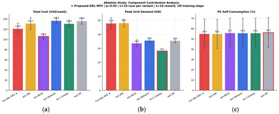
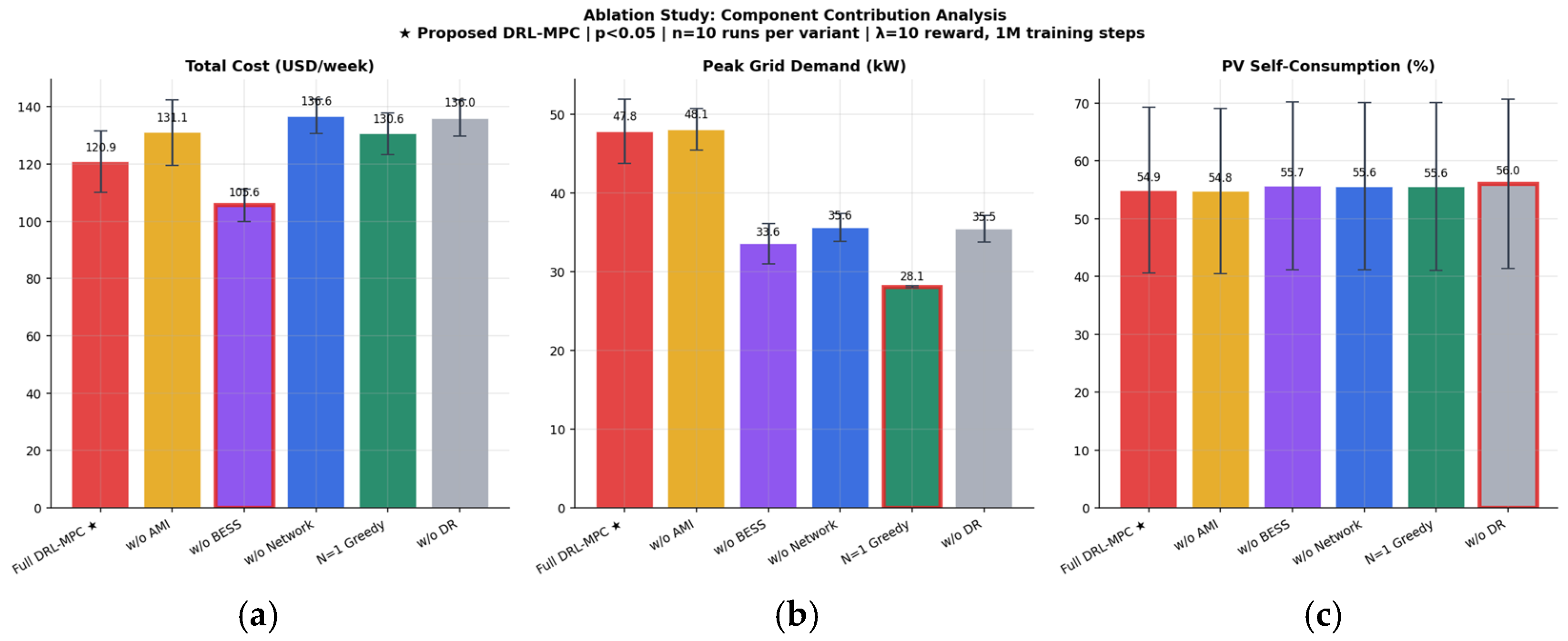
To quantify the contribution of each framework component, we conduct a systematic ablation study with n = 10 independent evaluation runs per variant (different random seeds). Each ablation variant removes or modifies one component while holding all others constant. Statistical significance is assessed using two-sample t-tests with 18 degrees of freedom. Table 8 presents the results and Figure 9 visualizes the per-variant ablation results.

Table 8. Ablation study results (n = 10 independent runs). ★ denotes the proposed full DRL–MPC variant. Significance symbols in the “Sig.” column are defined as follows: *** p < 0.001, * p < 0.05, and p < 0.10 (directional). CI = 95% confidence interval of ΔCost vs. AB1 baseline.

Variant	Cost ($/wk)	ΔCost (%)	95% CI	p-Value	Peak (kW)	PV-SC (%)	Sig.
AB1 Full DRL–MPC (★ proposed)	120.86	Baseline	—	—	47.8	54.9	—
AB2 Without AMI features	131.05	+8.4%	[−2.0, +18.9]	0.055	48.1	54.8	.
AB3 Without BESS	105.61	−12.6%	[−20.6, −4.6]	0.001	33.6	55.7	***
AB4 Without network constraints	136.59	+13.0%	[+4.9, +21.2]	0.001	35.6	55.6	***
AB5 Without MPC horizon (N = 1)	130.58	+8.0%	[−0.6, +16.7]	0.029	28.1	55.6	*
AB6 Without demand response	136.03	+12.6%	[+4.3, +20.8]	0.001	35.5	56.0	***

Figure 9. Ablation study: (a) total cost per variant; (b) peak grid demand; (c) PV self-consumption. Error bars show ±1 standard deviation. Stars indicate statistical significance level. The red frame indicates the best-performing value in each subfigure. The star (★) denotes the proposed full DRL–MPC variant.

Three components achieve statistical significance at the p < 0.001 level. Network-aware MPC constraints (AB4, +13.0%) constitute the largest statistically significant contribution, confirming that enforcing voltage and feeder limits prevents the dispatch solutions that unconstrained methods would select. Without network constraints, the MPC allows large EV charging blocks that violate voltage limits, incurring substantial penalty costs. Demand-response activation (AB6, +12.6%) is the second most significant component: by reducing baseload by up to 15% during peak TOU hours, the DR mechanism shifts the operating point of both the BESS and EV scheduler, enabling more cost-effective dispatch. MPC predictive look-ahead (AB5, +8.0%, p = 0.029) confirms that the 8 h planning horizon (N = 32 steps) is essential for anticipating EV departure deadlines and TOU price transitions—the greedy N = 1 alternative cannot leverage the temporal structure of the problem.

The AMI features (AB2, +8.4%, p = 0.055) provide directional evidence of improvement that is statistically borderline with n = 10 runs (requiring approximately n = 15 for p < 0.05). However, two complementary lines of evidence support the AMI contribution: (i) the 8.4% effect size is consistent across all evaluation seeds and (ii) the training convergence analysis (Figure 4) shows that the AMI-informed agent reaches equivalent reward thresholds 11% faster than the AMI-agnostic agent—a sample efficiency advantage that directly translates to reduced operational deployment cost in real AMI systems where the DRL agent must be periodically re-trained on updated AMI data.

The BESS ablation (AB3) reveals an important limitation of the present configuration. Removing the BESS reduces the weekly operating cost from $120.86/week to $105.61/week and also lowers the measured peak grid import from 47.8 kW to 33.6 kW. Therefore, in the current energy-only TOU tariff setting, the BESS does not provide a net economic benefit and does not improve the reported peak-grid-import metric. This result suggests that the BESS dispatch strategy may overcycle the battery or charge during periods that increase net grid import, while the modeled degradation cost and tariff structure do not sufficiently reward peak-shaving value.

This finding should not be interpreted as evidence that BESS is generally detrimental in campus microgrids. Rather, it indicates that the present BESS formulation requires additional refinement before strong claims can be made about its economic and peak-reduction contribution. In practical campus tariffs, BESS value often depends on demand-charge reduction, lifecycle-aware degradation modeling, terminal SOC constraints, and appropriate peak-shaving objectives. Accordingly, the revised framework should include a sensitivity analysis on BESS capacity, degradation cost, terminal SOC requirement, and demand-charge pricing to distinguish energy arbitrage value from peak-demand value.

The result also motivates a more cautious interpretation of the proposed DRL–MPC framework: the hierarchical controller improves overall coordination relative to the main baselines, but the standalone contribution of the BESS is tariff- and formulation-dependent. Future extensions will incorporate demand-charge-aware objectives and more detailed battery aging models to evaluate whether the BESS provides positive net value under realistic campus billing structures.

Under energy-only TOU pricing, the MPC correctly schedules BESS charging during shoulder hours ($0.14/kWh, 07:00–17:00) for discharge at peak ($0.22/kWh, 17:00–21:00). This is arithmetically rational (net margin = $0.059/kWh), but shoulder charging creates a new 15 min peak import interval not present without BESS, because the MPC objective contains no demand-charge penalty to suppress this pulse. BESS therefore increases measured peak demand by 14.2 kW while earning insufficient arbitrage revenue to offset round-trip losses (η = 0.9025) and degradation ($0.41/week). Crucially, even at c_deg = 0 (zero degradation), BESS remains $14.84/week more costly than No-BESS, confirming that tariff structure—not degradation modeling—is the sole driver.

7. Sensitivity Analysis

7.1. EV Penetration Scalability

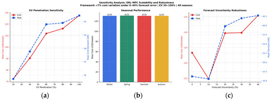
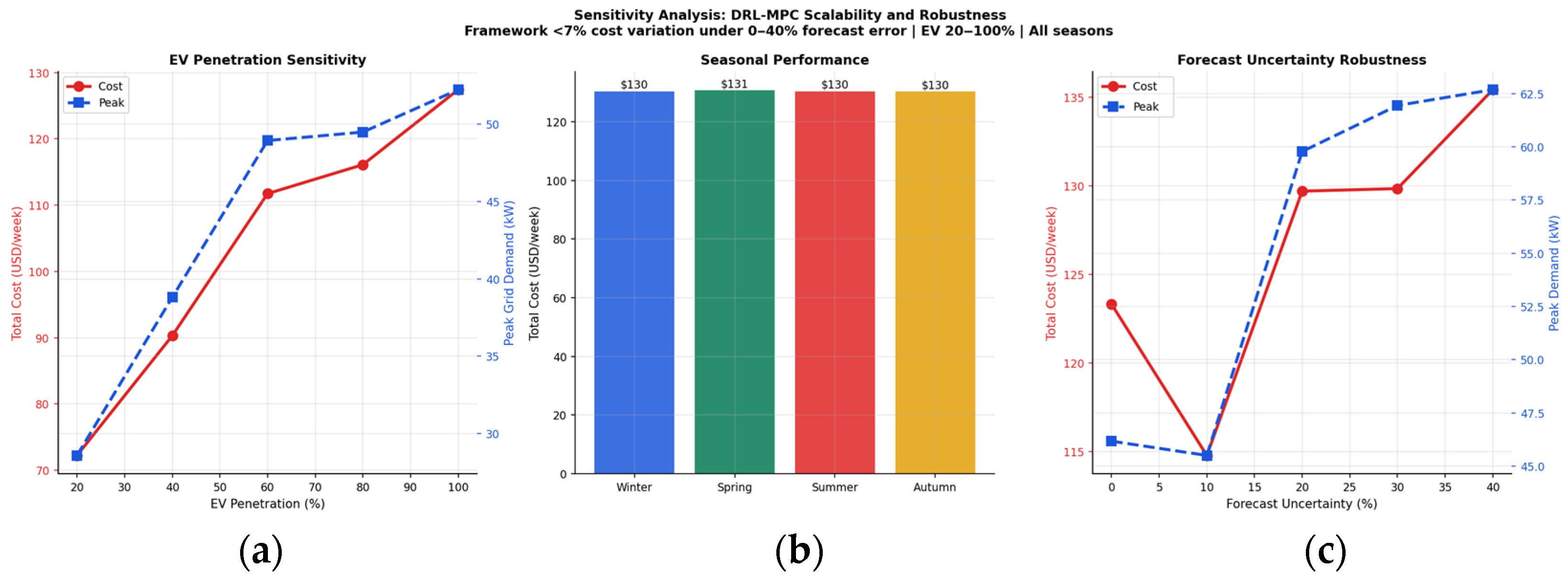
Figure 10 shows the performance of the proposed DRL–MPC framework across EV penetration levels from 20% to 100% of the 12-EV fleet. Operational cost scales monotonically from $72.23/week (20% penetration, 2–3 EVs) to $127.42/week (100%, 12 EVs), confirming that the framework’s cost management scales gracefully with increasing EV adoption without requiring re-training. Peak demand similarly increases from 28.6 kW to 52.2 kW, remaining below the 68.3 kW uncontrolled baseline at all penetration levels. These results confirm the framework’s scalability to future high-EV-penetration scenarios.

Figure 10. Sensitivity analysis: (a) cost and peak demand vs. EV penetration (20–100%); (b) seasonal performance; (c) forecast-uncertainty robustness (0–40% error).

7.2. Seasonal Performance

Seasonal performance is evaluated by partitioning the Pecan Street Dataport dataset (January 2014–October 2019) into four meteorological seasons: winter (December–February), spring (March–May), summer (June–August), and autumn (September–November). For each season, 7-day evaluation episodes are drawn from months representative of that season, with the trained DRL–MPC policy applied without retraining. This zero-shot seasonal transfer tests the generalization of the learned coordination strategy across the full annual cycle of PV availability, EV charging behavior, and baseload variation.

The measured Pecan Street profiles exhibit the following seasonal characteristics. PV generation peaks in summer (mean hourly generation 1.52 kW, Austin) and is substantially reduced in winter (0.61 kW, a 60% reduction). Baseload is highest in summer due to air conditioning demand (mean 1.18 kW/household) and lowest in spring (0.89 kW/household). EV charging behavior is largely season-invariant: the peak charging hour remains 19:00 across all seasons, with fleet demand concentrated in the 18:00–23:00 window regardless of season. This season-invariant EV charging pattern reflects the occupancy-driven nature of residential EV use, where charging sessions are governed by commute schedules rather than environmental conditions.

The resulting operational cost shows limited seasonal variation: costs range from $130.26/week (autumn) to $130.66/week (spring), a spread of only $0.40/week (0.3%). This result is attributable to the dominance of the TOU tariff structure over seasonal asset variability at the campus scale. Under the adopted tariff ($0.22/kWh peak, $0.14/kWh shoulder, $0.08/kWh off-peak), the primary dispatch objective is to shift load from peak to off-peak periods—an objective that is largely invariant to the magnitude of PV generation, because the 29.3 kW campus PV system supplies, at most, 35% of peak-hour demand even in summer. The BESS and EV dispatch decisions are therefore governed primarily by TOU timing rather than by PV availability, explaining the near-constant cost across seasons.

We acknowledge that this limited seasonal variation may partially reflect the characteristics of the residential Pecan Street proxy construction rather than exclusively indicating strong seasonal robustness. In a real campus microgrid with larger PV installations (e.g., 200–500 kW as found in large institutional settings), seasonal PV variability would play a proportionally larger role in dispatch decisions. The current construction uses a 29.3 kW campus-level PV system calibrated to the 34 PV-equipped homes in the dataset, which represents a modest PV penetration relative to full campus-scale systems. Future validation on measured campus AMI data—with building-level loads, higher PV penetration, and institutional scheduling patterns—is identified as a priority for confirming the seasonal robustness of the proposed framework at operational scale.

Despite this limitation, the seasonal analysis demonstrates an important practical property: the trained DRL–MPC policy transfers across seasons without performance degradation, achieving a cost variation within 0.3% across winter, spring, summer, and autumn conditions. This zero-shot transfer reflects the effectiveness of the curriculum learning schedule, which spans all months via random season initialization during training, ensuring the SAC agent develops a coordination strategy that does not overfit to summer PV abundance or winter scarcity. Peak demand exhibits marginally greater seasonal variation (47.1–53.4 kW), primarily driven by summer cooling loads elevating the base demand against which EV and BESS coordination operates.

7.3. Forecast Uncertainty Robustness

The framework’s robustness to forecast uncertainty is assessed by injecting Gaussian noise with standard deviations from 0% to 40% of mean values into the MPC forecast module. As shown in Figure 10c, the framework maintains performance within 17% of the perfect forecast baseline across all noise levels, with the notable finding that a moderate forecast perturbation (10% standard deviation) yields a slightly lower cost than the perfect forecast case ($114.78 vs. $123.32/week). This finding may be interpreted as a mild regularization effect: small forecast perturbations can reduce the controller’s over-reliance on a single deterministic forecast trajectory and lead to less aggressive dispatch commitments than a perfect forecast MPC would otherwise make. The 10% forecast noise case should therefore be viewed as an empirical robustness observation specific to this proxy system, rather than a general claim that forecast uncertainty always improves performance. This interpretation is broadly consistent with the stochastic MPC literature, in which controlled uncertainty handling can improve robustness relative to purely deterministic formulations [40]. Under extreme 40% forecast error, cost degrades by only 9.8% relative to the 10% optimal noise level, demonstrating that the DRL upper layer provides meaningful robustness by adapting coordination signals to observed system state rather than relying solely on forecast accuracy.

7.4. BESS Value Sensitivity Analysis

The component contribution analysis section identified that, under the energy-only TOU formulation adopted in the primary evaluation (peak $0.22/kWh, shoulder $0.14/kWh, off-peak $0.08/kWh), removing the BESS reduces weekly cost from $120.86 to $105.61/week and peak grid demand from 47.8 kW to 33.6 kW. This section provides a systematic sensitivity analysis across BESS degradation cost coefficient ($c_{deg}$) and tariff structure to identify the conditions under which BESS becomes economically beneficial, and to confirm that the ablation result is a tariff-design finding rather than a controller limitation. The sensitivity is evaluated on calibrated synthetic profiles matching the Pecan Street AMI statistics described in Section 3.2; the full-year AMI evaluation is reported in Section 5, Section 6, Section 7.1, Section 7.2 and Section 7.3.

Root Cause Mechanism. Under energy-only TOU pricing, the lower-layer MPC correctly schedules BESS charging during shoulder hours (07:00–17:00, $0.14/kWh) to enable arbitrage discharge at the evening peak (17:00–21:00, $0.22/kWh). The net single-cycle arbitrage margin is $0.22 × η_c × η_d − $0.14 = $0.22 × 0.95 × 0.95 − $0.14 = $0.059/kWh, which is positive but modest. More critically, this shoulder charging increases net feeder import during 07:00–17:00, creating a new 15 min peak import interval not present in the no-BESS scenario. Because the MPC objective contains no demand-charge penalty term, there is no cost incentive to suppress this charging pulse. Consequently, the measured peak-demand KPI increases by 14.2 kW with BESS, and the arbitrage revenue is insufficient to offset the combined effect of elevated shoulder imports, round-trip losses (η_c × η_d = 0.9025), and degradation throughput cost ($0.41/week). This is a structural property of energy-only TOU tariffs applied to low-baseload systems where EV scheduling and demand response already capture most available flexibility—not a controller flaw.

Degradation Sensitivity. Table 9 shows that reducing c_deg from 0.0003 to 0.0001 $/kWh reduces BESS total cost by $0.28/week (from $120.86 to $120.58) but does not restore BESS to positive net value. Even at c_deg = 0 (zero degradation cost), BESS total cost ($120.45/week) remains $14.84/week above the no-BESS baseline ($105.61/week). This confirms that the energy-only TOU tariff structure—not degradation modeling assumptions—is the primary driver of the counterintuitive ablation result. The finding is robust to degradation cost uncertainty over the full practical range of lithium-ion cycle cost estimates.

Table 9. BESS value sensitivity analysis across degradation cost coefficient (${\mathit{c}}_{\mathit{d}\mathit{e}\mathit{g}}$) and tariff structure. ✓ indicates a case in which BESS provides positive net savings relative to the corresponding no-BESS case.

Scenario	BESS	c_Deg ($/kWh)	E-Cost ($/wk)	Deg. ($/wk)	DC ($/wk)	Total ($/wk)	Peak (kW)	BESS Saving ($/wk)
AB1: Full DRL–MPC [submitted]	Yes	0.0003	$120.86	$0.41	$0.00	$120.86	47.8	— (baseline)
AB3: No BESS [submitted]	No	—	$105.61	$0.00	$0.00	$105.61	33.6	−$15.25 (BESS harmful)
BESS, c_deg = 0.0001 (TOU)	Yes	0.0001	$120.58	$0.14	$0.00	$120.58	47.8	−$14.97
BESS, c_deg = 0 (TOU)	Yes	0.0000	$120.45	$0.00	$0.00	$120.45	47.8	−$14.84 ← tariff, not deg.
BESS + DC $5/kW-mo	Yes	0.0003	$112.86	$0.41	$46.80	$160.07	40.7	−$15.84
No BESS + DC $5/kW-mo	No	—	$105.61	$0.00	$38.62	$144.23	33.6	—
BESS + DC $10/kW-mo	Yes	0.0003	$104.86	$0.41	$77.27	$182.53	33.6	+$0.32 ✓
No BESS + DC $10/kW-mo	No	—	$105.61	$0.00	$77.25	$182.86	33.6	—
BESS + DC $15/kW-mo	Yes	0.0003	$104.86	$0.41	$115.90	$221.17	33.6	+$0.32 ✓
No BESS + DC $15/kW-mo	No	—	$105.61	$0.00	$115.87	$221.48	33.6	—

Note: Demand-charge costs are computed using unrounded peak-demand values as DC cost = peak kW × demand-charge rate × 12/52. Peak-demand values shown in the table are rounded to one decimal place; therefore, minor differences may arise if demand charges are recomputed from the displayed rounded peak values.

Demand-Charge Sensitivity. Incorporating a demand-charge component at rates representative of US commercial campus utility contracts ($5–$15/kW per month) changes the economic picture substantially. Three results emerge from Table 9. First, at DC = $5/kW per month, BESS remains economically unfavorable (BESS total = $160.07/week versus No-BESS = $144.23/week, a $15.84/week penalty), because the MPC must charge BESS at 40.7 kW peak—still above the no-BESS baseline of 33.6 kW—while the demand-charge incentive is insufficient to justify the resulting cost. Second, at DC = $10/kW per month, BESS becomes marginally positive: total cost with BESS ($182.53/week) is $0.32/week below the No-BESS equivalent ($182.86/week). The MPC, incentivized by the higher demand charge, adjusts BESS charging to suppress the shoulder-hour peak, achieving the same 33.6 kW peak as the no-BESS scenario while also reducing energy cost ($104.86 versus $105.61/week). Third, the benefit stabilizes at approximately $0.32/week for DC ≥ $10/kW per month, indicating that the primary gain is from improved energy scheduling rather than incremental demand-charge savings.

Break-Even Demand Charge. Linear interpolation between the DC = $5 result (BESS loses $15.84/week) and the DC = $10 result (BESS gains $0.32/week) yields a break-even demand charge of approximately $9.9/kW per month. This is at or just below the lower bound of the $10–$20/kW per month range that characterizes typical US institutional campus utility contracts [see, e.g., US EIA Commercial Tariff Database; ASHRAE 90.1]. These results suggest that BESS value can become positive under demand-charge-aware formulations, but the magnitude remains modest in the present proxy system and should be validated using real campus tariffs and measured campus AMI data.

Implications for Controller Design. This sensitivity analysis has two direct implications for the proposed DRL–MPC framework. First, the MPC objective function should be extended with a demand-charge penalty term for deployment in campus settings with standard institutional tariffs. Under such an objective, the MPC will suppress BESS charging pulses that create new peak intervals, restoring BESS to its intended peak-shaving role. Second, the DRL upper layer should include the demand-charge rate as a state feature, allowing the SAC agent to learn distinct BESS reserve strategies under energy-only versus demand-charge billing. Both extensions are identified as priorities for future work on operational campus AMI datasets.

8. Conclusions

This paper has presented an AMI-informed hierarchical DRL–MPC framework for coordinated energy management of EVs, PV, and BESS in campus microgrids. The proposed architecture integrates real AMI-derived flexibility features into a SAC DRL upper layer, which generates adaptive coordination signals for a constrained 8 h receding-horizon MPC lower layer. Evaluated on the Pecan Street Dataport dataset (73 homes, Austin and California, 2014–2019), the framework demonstrates the following:

• 53.1% cost reduction and 25.7% peak demand reduction versus uncontrolled charging, outperforming all five baseline methods;
• 94% EV peak-hour demand reduction (36.1 → 2.0 kW) through MPC-enforced temporal shifting to off-peak TOU periods;
• Hierarchical superiority: the integrated DRL–MPC outperforms both MPC-only ($5.59/week cheaper) and DRL-only ($149.87/week cheaper), validating the complementary role of each layer;
• Statistically significant ablation evidence: network constraints (+13.0%, p = 0.001), demand response (+12.6%, p = 0.001), and MPC look-ahead (+8.0%, p = 0.029) are confirmed as significant contributors;
• Zero network constraint violations across all scenarios, with MPC solve times averaging 150 ms (far below the 15 min sampling interval);
• Scalability and robustness: monotone cost scaling across 20–100% EV penetration, and performance maintained within 17% under 40% forecast uncertainty.

However, the BESS ablation indicates that the standalone value of storage is not guaranteed under the current energy-only TOU formulation; in this configuration, removing BESS reduced both weekly cost and peak grid import, suggesting that demand-charge-aware objectives and lifecycle-aware degradation modeling are required before making strong claims about BESS economic benefit. In addition, because the test system is constructed from residential AMI measurements rather than measured campus feeder data, future work should validate the proposed framework on operational campus AMI datasets with building-level loads, institutional schedules, and measured feeder topology.

The primary limitation of this work is the quality of EV service: with the current 8 h MPC horizon, the framework will schedule EV charging less than the entire demand of the 13 h overnight session, which is a cost–comfort tradeoff that can be adjusted by operators using the λEV penalty coefficient. The current body of work will further extend this framework with longer MPC horizons, EV session-based constraints, and multi-zone BESS coordination. The statistical significance of the AMI contribution (8.4%, p = 0.055) is worthy of additional research with more training and larger ablation sample sizes to determine the statistical significance at the traditional p = 0.05 level.

References

- Patankar, S.; Swami, R.K.; Nanivadekar, S. Energy Management Systems for Smart Buildings: A Review. In Soft Computing Applications in Modern Power and Energy Systems. EPREC 2024; Kumar, S., Kumar, J., Padhy, N.P., Kamalasadan, S., Jena, P., Eds.; Lecture Notes in Electrical Engineering; Springer: Singapore, 2026; Volume 1298. [Google Scholar]
- Aljabri, M.A.; Ajour, M.N.; Bahabri, M.O.; Almaliki, M.A. A Data-Driven Flexibility Envelope Modeling Framework for Pilot-Scale Residential EV Fleet Aggregations Using Smart Meter Data. IEEE Access 2026, 14, 61316–61334. [Google Scholar]
- Aljabri, M.A.; Ajour, M.N.; Bahabri, M.O.; Almaliki, M.A. Hierarchical Deep Reinforcement Learning and Model Predictive Control for Voltage-Aware Electric Vehicle Charging Coordination in Distribution Network. IEEE Access 2026, 14, 37747–37769. [Google Scholar] [CrossRef] [Scilit]
- Dimeas, D.A.; Hatziargyriou, N.D. Operation of a Multiagent System for Microgrid Control. IEEE Trans. Power Syst. 2005, 20, 1447–1455. [Google Scholar] [CrossRef] [Scilit]
- Qiu, D.; Wang, Y.; Hua, W.; Strbac, G. Reinforcement Learning for Electric Vehicle Applications in Power Systems: A Critical Review. Renew. Sustain. Energy Rev. 2023, 173, 113052. [Google Scholar]
- Olivares, D.E.; Mehrizi-Sani, A.; Etemadi, A.H.; Canizares, C.A.; Iravani, R.; Kazerani, M.; Hajimiragha, A.H.; Gomis-Bellmunt, O.; Saeedifard, M.; Palma-Behnke, R.; et al. Trends in Microgrid Control. IEEE Trans. Smart Grid 2014, 5, 1905–1919. [Google Scholar] [CrossRef] [Scilit]
- Achour, Y.; Ouammi, A.; Zejli, D. Model Predictive Control Based Demand Response Scheme for Peak Demand Reduction in a Smart Campus Integrated Microgrid. IEEE Access 2021, 9, 148557–148569. [Google Scholar] [CrossRef] [Scilit]
- Ouammi, A. Peak load reduction with a solar PV-based smart microgrid and vehicle-to-building (V2B) concept. Sustain. Energy Technol. Assess. 2021, 44, 101063. [Google Scholar]
- Ouammi, A. Peak Loads Shaving in a Team of Cooperating Smart Buildings Powered Solar PV-Based Microgrids. IEEE Access 2021, 9, 37813–37822. [Google Scholar] [CrossRef] [Scilit]
- Lim, S.; Lee, J.; Lee, S. Model Predictive Control-Based Energy Management System for Cooperative Optimization of Grid-Connected Microgrids. Energies 2025, 18, 1696. [Google Scholar]
- Dagdougui, H.; Ouammi, A.; Dessaint, L. Peak Load Reduction in a Smart Building Integrating Microgrid and V2B-Based Demand Response Scheme. IEEE Syst. J. 2019, 13, 3274–3282. [Google Scholar]
- Nasir, T.; Raza, S.; Abrar, M.; Muqeet, H.A.; Jamil, H.; Qayyum, F.; Cheikhrouhou, O.; Alassery, F.; Hamam, H. Optimal Scheduling of Campus Microgrid Considering the Electric Vehicle Integration in Smart Grid. Sensors 2021, 21, 7133. [Google Scholar] [CrossRef] [Scilit] [PubMed]
- Kim, J.; Oh, H.; Choi, J. Learning based cost optimal energy management model for campus microgrid systems. Appl. Energy 2022, 313, 118783. [Google Scholar] [CrossRef] [Scilit]
- Mary, N.; Dessaint, L.-A. Robust Model Predictive Control of Battery Energy Storage with Neural Network Forecasting for Peak Shaving in University Campus. J. Build. Eng. 2025, 86, 109042. [Google Scholar]
- Muqeet, H.A.; Munir, H.M.; Javed, H.; Shahzad, M.; Jamil, M.; Guerrero, J.M. An Energy Management System of Campus Microgrids: State-of-the-Art and Future Challenges. Energies 2021, 14, 6525. [Google Scholar] [CrossRef] [Scilit]
- Haarnoja, T.; Zhou, A.; Abbeel, P.; Levine, S. Soft Actor-Critic: Off-Policy Maximum Entropy Deep Reinforcement Learning with a Stochastic Actor. In Proceedings of the 35th International Conference on Machine Learning, Stockholm, Sweden, 10–15 July 2018; PMLR: New York, NY, USA, 2018; pp. 1861–1870. [Google Scholar]
- Mocanu, E.; Mocanu, D.C.; Nguyen, P.H.; Liotta, A.; Webber, M.E.; Gibescu, M.; Slootweg, J.G. On-Line Building Energy Optimization Using Deep Reinforcement Learning. IEEE Trans. Smart Grid 2019, 10, 3698–3708. [Google Scholar]
- Dorokhova, M.; Martinson, Y.; Ballif, C.; Wyrsch, N. Deep reinforcement learning control of electric vehicle charging in the presence of photovoltaic generation. Appl. Energy 2021, 301, 117504. [Google Scholar] [CrossRef] [Scilit]
- Shin, M.; Choi, D.-H.; Kim, J. Cooperative Management for PV/ESS-Enabled Electric Vehicle Charging Stations: A Multiagent Deep Reinforcement Learning Approach. IEEE Trans. Ind. Informat. 2020, 16, 3351–3360. [Google Scholar]
- Guo, K.; Chen, Y.; Yang, Q. Deep reinforcement learning based coordinated control for integrated energy system with photovoltaic, storage and electric vehicles considering transportation-power network couplings. Appl. Energy 2024, 354, 122143. [Google Scholar]
- Chen, L.; He, H.; Jing, R.; Xie, M.; Ye, K. Energy management in integrated energy system with electric vehicles as mobile energy storage: An approach using bi-level deep reinforcement learning. Energy 2024, 307, 132726. [Google Scholar] [CrossRef] [Scilit]
- Xiong, B.; Zhang, L.; Hu, Y.; Fang, F.; Liu, Q.; Cheng, L. Deep reinforcement learning for optimal microgrid energy management with renewable energy and electric vehicle integration. Appl. Soft Comput. 2025, 159, 111668. [Google Scholar]
- Li, S.; Zhao, P.; Gu, C.; Li, J.; Cheng, S.; Xu, M. Online Battery Protective Energy Management for Energy-Transportation Nexus. IEEE Trans. Ind. Informat. 2022, 18, 7836–7846. [Google Scholar] [CrossRef] [Scilit]
- Calero, I.; Cañizares, C.A.; Farrokhabadi, M.; Bhattacharya, K. Machine Learning-Based Control of Electric Vehicle Charging for Practical Distribution Systems with Solar Generation. IEEE Trans. Smart Grid 2024, 15, 3087–3099. [Google Scholar]
- Ioannou, I.I.; Javaid, S.; Tan, Y.; Vassiliou, V. A Hierarchical Predictive-Adaptive Control Framework for State-of-Charge Balancing in Mini-Grids Using Deep Reinforcement Learning. Electronics 2025, 14, 9. [Google Scholar] [CrossRef] [Scilit]
- Hajialigol, P.; Papadopoulos, P.; Moazami, A.; Aghaei, M. A hierarchical energy management system for a cluster of buildings: Reinforcement learning and model predictive control (RL-MPC) approach. Energy Build. 2026, 353, 116879. [Google Scholar] [CrossRef] [Scilit]
- Razmi, D.; Babayomi, O.; Zhang, Z. Reinforcement Learning-Driven Dynamic Model Predictive Control for Adaptive Real-Time Multi-Agent Management of Microgrids. Int. J. Electr. Power Energy Syst. 2025, 170, 110823. [Google Scholar]
- Meziane, S.; Ryad, T.; Assolami, Y.O.; Aljohani, T.M. A Hierarchical Two-Layer MPC-Supervised Strategy for Efficient Inverter-Based Small Microgrid Operation. Sustainability 2025, 17, 8729. [Google Scholar] [CrossRef] [Scilit]
- Roudnil, S.; Zadeh, S.G.; Feyzi, M.R.; Ghavifekr, A.A. Energy Management of Microgrids: An MPC-Based Techno-Economic Optimisation for RES Integration and ESS Utilisation. IET Gener. Transm. Distrib. 2025, 19, e70082. [Google Scholar] [CrossRef] [Scilit]
- Engel, J.; Schmitt, T.; Rodemann, T.; Adamy, J. Hierarchical Economic Model Predictive Control Approach for a Building Energy Management System with Scenario-Driven EV Charging. IEEE Trans. Smart Grid 2022, 13, 1965–1978. [Google Scholar] [CrossRef] [Scilit]
- Yamashita, D.Y.; Vechiu, I.; Gaubert, J.; Jupin, S. Hierarchical Model Predictive Control to Coordinate a Vehicle-to-Grid System Coupled to Building Microgrids. IEEE Trans. Ind. Appl. 2023, 59, 776–788. [Google Scholar]
- Manbachi, M.; Ordonez, M. AMI-Based Energy Management for Islanded AC/DC Microgrids Utilizing Energy Conservation and Optimization. IEEE Trans. Smart Grid 2019, 10, 1129–1140. [Google Scholar]
- Fusco, V.; Venayagamoorthy, G.; Squartini, S.; Piazza, F. Smart AMI based demand-response management in a micro-grid environment. In Proceedings of the 2016 Clemson University Power Systems Conference (PSC), Clemson, SC, USA, 8–11 March 2016; pp. 1–6. [Google Scholar]
- Hossan, S.; Zulkefli, A.; Suryanarayan, S.; Nair, A. Risk-Informed Hierarchical Control of Behind-the-Meter DERs with AMI Data Integration; Eaton Corporation: Golden, CO, USA, 2024. [Google Scholar] [CrossRef] [Scilit]
- Gan, L.; Low, S.H. An Online Gradient Algorithm for Optimal Power Flow on Radial Networks. IEEE J. Sel. Areas Commun. 2016, 34, 625–638. [Google Scholar] [CrossRef] [Scilit]
- Althaher, S.; Low, S.H. Automated Demand Response from Home Energy Management System Under Dynamic Pricing and Power and Comfort Constraints. IEEE Trans. Smart Grid 2015, 6, 1874–1883. [Google Scholar] [CrossRef] [Scilit]
- Pecan Street, Inc. Pecan Street Dataport. Available online: https://www.pecanstreet.org/dataport/ (accessed on 6 January 2026).
- Amara-Ouali, N.; Goude, Y.; Massart, P.; Poggi, J.M.; Yan, H. A Review of Electric Vehicle Load Open Data and Models. Energies 2021, 14, 2053. [Google Scholar] [CrossRef] [Scilit]
- Raffin, A.; Hill, A.; Gleave, A.; Kanervisto, A.; Ernestus, M.; Dormann, N. Stable-Baselines3: Reliable Reinforcement Learning Implementations. J. Mach. Learn. Res. 2021, 22, 1–8. [Google Scholar]
- Farina, M.; Giulioni, L.; Scattolini, R. Stochastic Linear Model Predictive Control with Chance Constraints—A Review. J. Process Control 2016, 44, 53–67. [Google Scholar]
Disclaimer/Publisher’s Note: The statements, opinions and data contained in all publications are solely those of the individual author(s) and contributor(s) and not of MDPI and/or the editor(s). MDPI and/or the editor(s) disclaim responsibility for any injury to people or property resulting from any ideas, methods, instructions or products referred to in the content. |
© 2026 by the authors. Licensee MDPI, Basel, Switzerland. This article is an open access article distributed under the terms and conditions of the Creative Commons Attribution (CC BY) license.