ML-Based Feasibility-Prediction for NB-IoT Smart Metre Deployment in Thailand: A Cross-Environment Multi-Site Study

Abstract

Thailand’s Provincial Electricity Authority (PEA) is rolling out Advanced Metering Infrastructure (AMI) under its smart-grid initiative, requiring a reliable last-mile wireless network across heterogeneous propagation environments. Narrowband IoT (NB-IoT) is a leading candidate, but per-area deployment decisions have lacked a data-driven framework anchored to measured Thai propagation. Building on our sixteen-site composite-channel characterisation, this study presents a machine-learning feasibility-prediction framework integrating measured channel parameters (n, σ_sh, $\widehat{m}$), an OpenStreetMap-derived synthetic meter-density layer, and a benchmark of Random Forest, Gradient Boosting (GB), and Multi-Layer Perceptron classifiers trained on Monte-Carlo coverage labels to predict 95% RSRP-coverage feasibility per spatial cell. Across 411 cells from four Thai sites spanning Urban Dense, Urban Outdoor, Suburban, and Rural environments, GB achieves accuracy 0.971 and F1 0.969 at 1.7 ms inference latency—four orders of magnitude faster than direct Monte-Carlo simulation. The ML predictor approximates the Monte-Carlo engine under the assumed composite-channel model. A theoretical LPWAN comparison places NB-IoT as recommended for Suburban and Rural AMI; Suphan Buri (Rural) is the only RECOMMENDED case (88.5% cells feasible), with hybrid PLC backhaul suggested for dense urban areas.

1. Introduction

Building on our recent sixteen-site NB-IoT propagation characterisation in Thailand [1], this study addresses the operational feasibility of large-scale NB-IoT-based Advanced Metering Infrastructure (AMI) deployment for the Provincial Electricity Authority. The Provincial Electricity Authority (PEA) of Thailand is transitioning from conventional power distribution to a digitally instrumented Smart Grid utility under its ‘PEA Digital Utility’ programme [2]. A foundational layer of this transition is Advanced Metering Infrastructure (AMI)—bidirectional, low-latency, low-power telemetry from millions of consumer endpoints back to distribution-management systems. The wireless last-mile to those metres must deliver three properties simultaneously: (i) deep-indoor reach, since metres are installed inside electrical cabinets, behind walls, or in basements; (ii) long battery life, with utility metres targeting 10–15 year service intervals; and (iii) operator-managed reliability with service-level agreements that survive multi-vendor rollouts.

Narrowband Internet of Things (NB-IoT), standardised in 3GPP Release 13/14 [3,4], was designed precisely against this profile. In Thailand, AIS (Band 8, 900 MHz) and True Corporation (Band 8/Band 28) operate nationwide NB-IoT networks. Yet a site-specific deployment decision—will NB-IoT serve the metres in this area at the required reliability, and how does it compare to the alternatives such as LoRaWAN, ZigBee, or Power-Line Communication (PLC)?—has remained under-supported by published Thai-specific evidence.

1.1. Companion Channel-Characterisation Study

Our companion channel-characterisation study [1], extending the earlier conference work [5], reported a composite-channel characterisation of NB-IoT for sixteen sites across five environment classes in central and western Thailand. Each environment was assigned back-calculated parameters: path-loss exponent n, log-normal shadowing standard deviation σ_sh, and Nakagami-m fading parameter obtained via a σ-decomposition methodology. The principal findings establish the channel-parameter inputs that this framework consumes.

The prior study established class-specific values for n, σ_sh, and $\widehat{m}$ across five environment classes, summarised in Table 1. That study ended with environment-class-level statistics that are useful for high-level planning but not yet directly applicable to a specific PEA service area—the gap that this paper closes.

Table 1. Composite-channel parameters per environment class established by the companion study [1] (16 sites grouped into 5 classes). These class-average parameters feed the Monte-Carlo coverage labelling of Section 2.4.

Environment Class	Sites (J1)	n	σsh (dB)	$\widehat{\mathit{m}}$	Notes
Urban Dense	01–02	3.50	8.5	1.00	Rayleigh fading
Urban Outdoor	03–06	3.00	7.25	1.25	Weak Rician (K ≈ −0.5 dB)
Suburban	07–09	2.65	6.75	1.84 ± 0.57	Intra-class variance reflects suburban heterogeneity
Rural	10–13	2.20	4.65	2.50	Near-Rician
Forest/Mountain	14–16	4.00	8.5–9.2	0.44–0.62	Outage Pout = 3.4–24.7% from terrain blockage

1.2. Contributions of This Paper

This paper closes the application gap by asking: given an area of interest in Thailand, can NB-IoT support PEA’s AMI rollout there at a 95% RSRP-coverage target, and how does NB-IoT compare against alternative LPWAN technologies for that same area? Three contributions answer this question.

First, we present a Thailand-specific ML feasibility-prediction framework that integrates a reproducible synthetic-GIS pipeline (OpenStreetMap building footprints → metre-density layer) with Monte-Carlo coverage labels parameterised by the channel measurements of [1]—usable without access to PEA’s restricted operational GIS.

Second, we benchmark three machine-learning algorithms (Random Forest, Gradient Boosting, Multi-Layer Perceptron) under stratified 5-fold cross-validation on 411 Monte-Carlo-labelled cells across four environment classes; Gradient Boosting attains F1 = 0.969 with inference latency ≈ 1.7 ms per cell, four orders of magnitude faster than direct Monte-Carlo simulation.

Third, we develop a published-parameter LPWAN scoring rubric and a per-site verdict logic that translate the ML output and channel parameters into a deployable per-area recommendation, exercised on four Thai case-study sites spanning Urban Dense, Urban Outdoor, Suburban, and Rural environments.

1.3. Comparison with Prior ML-Coverage Prediction Works

ML-based coverage prediction from spatial features has been explored using satellite imagery [6] and geographic features [7]. The present work draws on these established components (OSM-derived synthetic GIS, Monte-Carlo coverage labels, supervised ML classification) and constitutes an engineering-integration contribution rather than a methodological breakthrough in any single ingredient. Three deliberate design choices distinguish our framework: (i) the first Thailand-specific integration of measured local channel parameters from a sixteen-site companion study [1]; (ii) explicit per-area feasibility verdicts (RECOMMENDED/MARGINAL/NOT-RECOMMENDED) targeted at AMI deployment decisions rather than the cell coverage heat-maps that prior ML-coverage works typically produce; and (iii) integration of an LPWAN-comparison rubric spanning six radio-access technologies (NB-IoT, LTE-M, LoRaWAN, Sigfox, ZigBee, PLC G3-PLC)—an extension beyond ML-coverage-only studies.

Section 2 details the methodology—pipeline architecture, case-study sites, synthetic metre-density extraction, ML algorithm benchmark, and the LPWAN technology comparison rubric. Section 3 presents per-site results, the cross-site summary, the multi-site ML benchmark, and the LPWAN scoring per environment. Section 4 discusses why ML adds value over direct Monte-Carlo, threshold sensitivity, why NB-IoT can lose on raw rubric scores, and the asymmetry between the deeply characterised NB-IoT channel and the literature-only comparator technologies. Section 5 concludes.

2. Materials and Methods

2.1. Pipeline Architecture

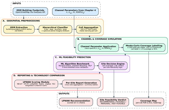
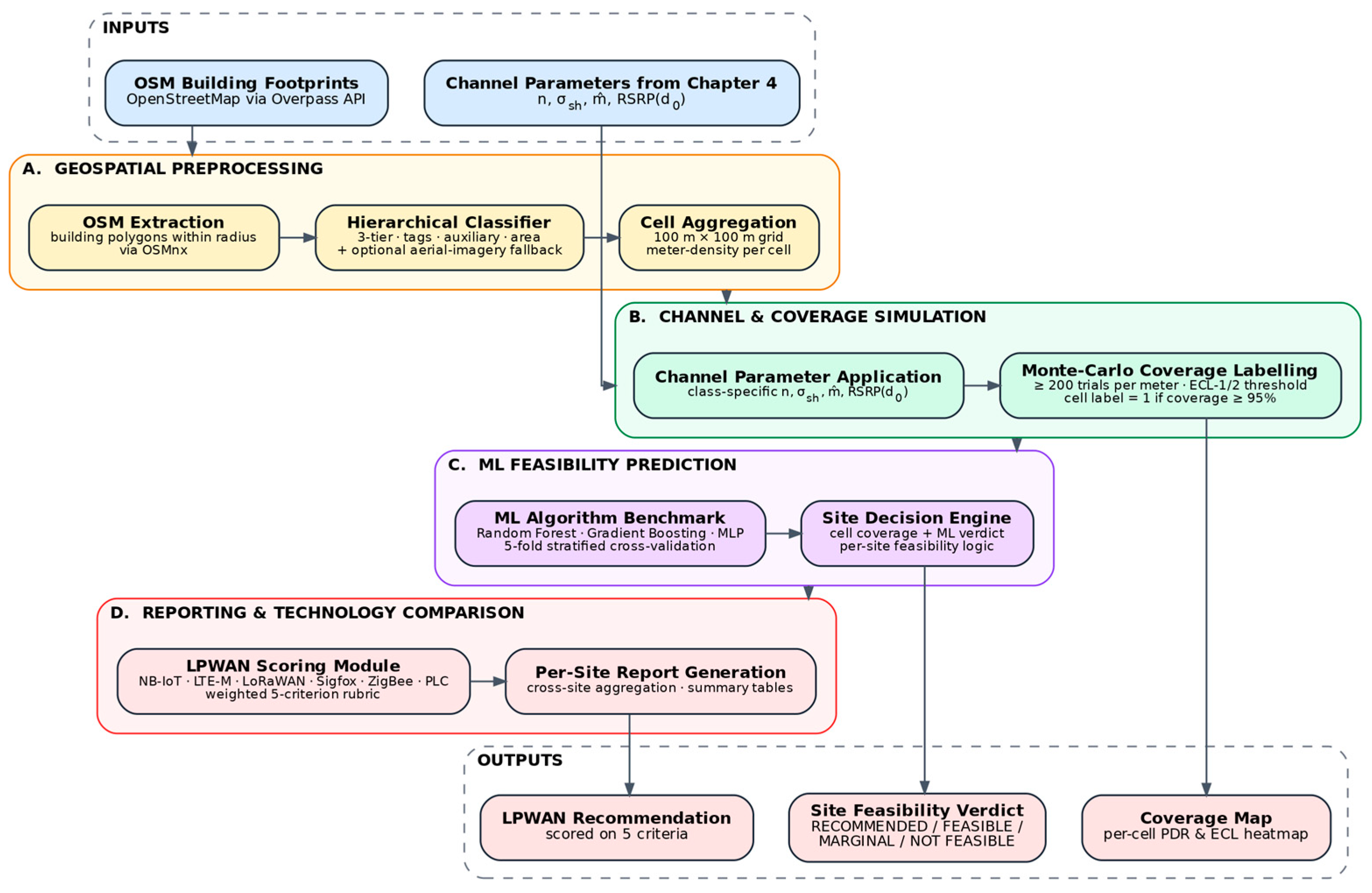
The framework is realised as four cascaded stages, summarised in Figure 1. The geospatial preprocessing stage builds the synthetic metre-density layer from OSM building footprints. The coverage-simulation stage generates per-cell Monte-Carlo coverage labels using the channel parameters of [1]. The machine-learning stage trains and benchmarks three classifiers against the labelled cells. Finally, the reporting and technology-comparison stage scores candidate LPWAN technologies on a published-parameter rubric and aggregates the outputs into a deployable per-area feasibility report. All data processing, machine-learning training, and simulation were implemented in Python 3.11 (Python Software Foundation, Beaverton, OR, USA).

Figure 1. End-to-end AI-assisted feasibility pipeline. OSM building data and the channel parametres from [1] feed the synthetic meter-density layer; Monte-Carlo coverage labels train the ML predictor; the LPWAN rubric and feasibility report close the loop.

2.2. Case-Study Site Selection

Four sites are drawn from the sixteen-site dataset of [1], chosen to span the residential-metre-density spectrum that PEA’s AMI rollout must serve. Table 2 lists the four sites with their inherited class-average channel parameters from [1].

Table 2. Case-study sites for Section 3, with class-average channel parameters inherited from [1].

#	Site (Academic Name)	Env Class	n	σsh	$\widehat{\mathit{m}}$	Centre (Lat, Lon)	Radius (m)
1	Pracharat Rd. Wongsawang, BKK	Urban Dense	3.5	8.5	1.00	(13.8195, 100.5145)	800
2	Phet Kasem Rd. Bang Wa, BKK	Urban Outdoor	3.0	7.25	1.25	(13.7178, 100.4533)	1000
3	Nakhon Pathom Residential, NPT	Suburban	2.65	6.75	1.84	(13.8190, 100.0700)	1200
4	Suphan Buri City Centre, SPB	Rural	2.2	4.65	2.50	(14.4744, 100.1188)	2500

2.3. Synthetic Metre-Density Pipeline

2.3.1. OSM Building Extraction

The OSM extraction module uses the OSMnx library (version 1.9.4, open-source Python package by G. Boeing, University of Southern California, Los Angeles, CA, USA) [8] to download building polygons within a configurable circular radius around a candidate-area centre. The output comprises a GeoJSON file, a tabular CSV with centroid latitude/longitude, a metadata JSON, and a quick-look map. The radius is chosen per environment class—800 m for Urban Dense, 1000 m for Urban Outdoor, 1200 m for Suburban, and 2500 m for Rural—to match typical NB-IoT cell coverage.

2.3.2. Hierarchical Building Classification

A three-tier hierarchical classifier assigns each building polygon to one of {residential, commercial, industrial, institutional, auxiliary, unknown}. Tier 1 maps the OSM ‘building=’ tag directly to a category; Tier 2 disambiguates ‘building = yes’ rows via auxiliary tags (amenity, shop, office, tourism); Tier 3 falls back to a footprint-area heuristic calibrated for Thai urban morphology (≤250 m² → residential; >1000 m² → flagged for aerial-image classification). When the Tier-3 unknown rate exceeds 20%, an optional aerial-imagery classifier—currently a stochastic placeholder, replaceable in future work by a CNN trained on Microsoft Building Footprints—is invoked as a fallback. Quantitatively, the Tier-3 unknown rate ranges 14–29% across the four sites; a sensitivity sweep performed in this revision (Section 3.5.5) recomputed metre counts under ±20% perturbation and found median verdict change of <8% (no site reclassified across the RECOMMENDED/MARGINAL/NOT-RECOMMENDED boundary), indicating the framework is robust to plausible OSM-density error.

2.3.3. Metre-Count Estimation

The metre-count estimator translates each classified building into a number of electricity metres using the rules summarised in Table 3.

Table 3. Metre-count estimation rules per building category. A = footprint area, L = number of building levels.

Category	Metre Count Rule	AMI Priority
Single-family residential	1 m	high
Multi-family (apartments)	max(1, ⌈L × A/50 m2⌉)	high
Commercial (small)	max(1, ⌈L × A/150 m2⌉)	medium
Hotel	max(1, ⌈A/25 m2⌉)	medium
Industrial	1 high-power metre	low
Institutional	1 m	low
Other/Auxiliary	0	none
Unknown	1 (conservative)	unknown

2.4. Coverage Labelling and Feature Engineering

The coverage-labelling stage divides the candidate area into a 100 m × 100 m grid. The cell size matches the shadow-fading decorrelation distance [9] and ensures each cell typically contains at least one building, while remaining computationally tractable for 200-trial Monte-Carlo simulation [9,10]. The composite-channel model of [1] is then evaluated per metre:

RSRP(d) = RSRP_d0 − 10 n log₁₀(d/d0) + X_sh + X_fade

(1)

Here RSRP(d0) denotes the reference received power at the close-in reference distance d0 (taken as d0 = 1 m in the companion study [1]); X_sh and X_fade are the dB-domain shadow-fading and Nakagami-fading random variables respectively (see the derivation below).

With X_sh~N(0, σ_sh²) in dB and X_fade a zero-mean Nakagami-$\widehat{m}$ [11] random variable in dB, both as defined in Equations (1) and (2). The cell coverage percent is the fraction of all (metre × Monte-Carlo) realisations whose RSRP exceeds the configurable threshold T (default −105 dBm—the ECL-1/2 boundary established in [1]). The cell label is y = 1 (feasible) if coverage ≥ 95%, otherwise y = 0.

Nakagami-m fading is conventionally defined in the linear amplitude domain with envelope density f_r(r) = (2 m^m/Γ(m) Ω^m) r^(2 m-1) exp(−m r²/Ω), where Ω = E[r²]. To align with the dB-domain RSRP variable, X_fade = 10 log₁₀(r²/Ω) − μ_X($\widehat{m}$), where μ_X($\widehat{m}$) = (10/ln 10)(ψ($\widehat{m}$) − ln $\widehat{m}$) is the Jensen-correction term ensuring E[X_fade] = 0 (ψ denoting the digamma function). The variance is Var(X_fade) = (10/ln 10)² · ψ’($\widehat{m}$), where ψ’ is the trigamma function. For our class-specific $\widehat{m}$ ∈ {1.00, 1.25, 1.84, 2.50} from Table 1 of [1], the per-sample fading variances evaluate to ≈31, 19, 12, and 8 dB² respectively—comparable in magnitude to σ_sh² (21.6–72.3 dB²). At cell coverage level, spatial averaging across the metres reduces per-metre variance to below 1 dB² for N_meters ≥ 10, so the deterministic path-loss and shadow-fading components dominate after Monte-Carlo aggregation.

The 95% coverage threshold follows cellular-planning practice: a 95% point-coverage probability corresponds to a 1.645·σ_sh shadow margin [9], underpins the 164 dB MCL specification for NB-IoT in 3GPP TR 45.820 [4], and is consistently adopted as the design KPI in the NB-IoT design and field-measurement literature [12,13]. From the AMI side it aligns with billing-grade reliability for DLMS/COSEM-based metering [14]. Section 4.2 reports a sensitivity sweep over stricter (99%) and looser (80%) targets.

Each cell becomes one supervised-learning example with the fifteen-dimensional feature vector listed in Table 4: building and metre counts (5 features), category share fractions (4 features), area summaries (2 features), distance to centre (1 feature), and the four channel parameters (n, σ_sh, $\widehat{m}$, RSRP_d0) inherited from [1] (4 features).

Table 4. Cell-level feature vector for the ML feasibility predictor (15 features in total).

Feature	Description
n_buildings	Number of buildings within the cell
meterstotal/high/medium	Total/high-priority/medium-priority metre counts
share_residential/commercial/institutional/unknown	Building-category share fractions
mean_building_area_m2/total_floor_area_m2	Mean and total floor area
distance_to_centre_m	Distance from cell centre to BS
nlit, σ_sh_dB, m_nakagami, RSRP_d0_dBm	Channel parameters from [1]

2.5. ML Algorithm Benchmark

Three classifiers from distinct inductive-bias regimes are benchmarked using the scikit-learn library (version 1.4, open-source Python machine-learning library, https://scikit-learn.org) [15]: Random Forest (RF) for variance-reduction by ensembling, Gradient Boosting (GB) for bias-reduction by sequential residual fitting, and a Multi-Layer Perceptron (MLP) for non-linear function approximation. Each algorithm is summarised below by its principal equation and chosen hyperparameters; full theoretical treatments are available in the scikit-learn documentation and the standard machine-learning literature. During implementation, an AI-assisted code review and editing workflow (Anthropic Claude, Anthropic PBC, San Francisco, CA, USA) was used for scikit-learn pipeline development and verification of the cross-validation protocol; all model hyperparameters, feature-engineering decisions, and reported results were defined, executed, and verified by the authors.

2.5.1. Random Forest Classifier

A Random Forest is an ensemble of B = 200 decision trees, each grown on an independent bootstrap sample of the training set with √p ≈ 4 random-feature subsetting per split (p = 15 features). Predictions aggregate via majority vote:

ŷ_RF(x) = mode {T_b(x): b = 1, …, B}

(2)

Bagging plus random-feature subsetting decorrelates the trees so the ensemble has lower variance than any single tree without inflating bias. The native impurity-based feature importance also provides direct interpretation of which inputs drive the verdict (reported in Section 3.5.1).

2.5.2. Gradient Boosting Classifier

Gradient Boosting builds an additive model by sequentially fitting a shallow tree h_m to the negative gradient of the loss at iteration m:

F_m(x) = F_{m-1}(x) + ν · h_m(x)

(3)

with learning rate ν = 0.05, per-tree depth capped at 4, and M = 200 boosting stages; an early-stopping check confirmed validation log-loss converged by M ≈ 180. Compared with Random Forest, GB trades parallelism for typically lower bias on tabular feature interactions.

2.5.3. Multi-Layer Perceptron Classifier

The MLP is a feed-forward network with two hidden layers (64 and 32 units, ReLU activation) and a sigmoid output for binary classification:

ŷ = σ(W₃ · ReLU(W₂ · ReLU(W₁ x + b₁) + b₂) + b₃)

(4)

The (64, 32) hidden-layer width yields ~3100 weights—approximately 7.5× the 411-sample training-set size; to mitigate overfitting under this ratio we rely on Adam optimisation with internal early stopping, feature standardisation, and the regularising effect of stratified cross-validation. The LOSO results in Section 3.5.3 confirm the model has not memorised within-site spatial structure beyond reasonable bounds. Training minimises binary cross-entropy with the Adam optimiser (default scikit-learn hyperparameters, 500-epoch cap with internal early-stopping); features are standardised to zero mean, unit variance before training. The MLP serves as a non-linear, non-tree-based baseline whose globally smooth decision surface contrasts with the trees’ axis-aligned partitions.

2.5.4. Cross-Validation Protocol and Performance Metrics

All three algorithms are evaluated by stratified 5-fold cross-validation, preserving the 193:218 class balance in each fold. Three metrics are reported as mean ± std across folds: classification accuracy, the macro F1 score (which penalises majority-class bias), and ROC-AUC (a threshold-independent measure of separability). Inference latency on a single full-data fit is also measured as the operationally relevant figure for PEA-scale deployment.

2.6. LPWAN Technology Comparison

Six radio-access technologies are scored on a five-component weighted rubric: NB-IoT [13,16,17] and LTE-M (Cat-M1) [3,13,18] from the cellular family; LoRaWAN [19,20,21] and Sigfox [20] as unlicensed LPWAN; ZigBee/IEEE 802.15.4 [20] as short-range mesh; and Power-Line Communication (G3-PLC) [22] as wireline last-mile. This rubric is presented as a transparent qualitative screening tool for cross-technology orientation, not as a quantitative deployment ranking; the weighting choices and source asymmetry are revisited in Section 4.3 and Section 4.4.

S = 0.25·s_range + 0.25·s_pen + 0.20·s_bat + 0.15·s_scal + 0.15·s_lat

(5)

Each sub-score is normalised to 0–100 against engineering target ideals representative of utility-grade AMI deployment: range (target 2 km urban, 5 km suburban, 10 km rural), deep-indoor penetration (target 20 dB), battery life (target 10 years), scalability (target 10,000 devices/cell), and end-to-end latency (target ≤ 10 s). The 0.25/0.25 weights on range and penetration reflect the hard deployability constraints—a technology that fails to reach the metre cannot be deployed regardless of other merits—while the remaining 0.50 weight covers operational metrics. Each cell of the comparison table is anchored to a published reference [19,20,21,22].

An asymmetry in data sources is acknowledged: NB-IoT parameters draw on the 16-site Thai measurement campaign of [1] and operator-grade surveys [,16], whereas the other technologies are anchored to single-region or single-environment studies—Petajajarvi et al. [20] for LoRaWAN in Finland, Kongsavat and Karupongsiri [21] for LoRaWAN in a single Thai suburban site, Centenaro et al. [20] for Sigfox/ZigBee, and Galli et al. [22] for PLC. The rubric therefore serves as a transparent, reproducible first-pass screening framework: it identifies dominant deployability constraints across six technologies and supports cross-technology orientation, with numerical sub-scores interpretable to within ±5–10 score units. Region-specific field validation is required before committing to a deployment decision; this limitation is revisited in Section 4.3 and Section 4.4.

2.7. Per-Site Feasibility Verdict

The per-site report generator aggregates the outputs of the coverage-simulation, machine-learning, and LPWAN-comparison stages into a single deployable report (Table 5). The verdict combines two thresholds: an area-coverage threshold of ≥80% feasible cells, and an LPWAN-suitability threshold of ≥60 (out of 100) for NB-IoT. The 80% area threshold reflects the two-tier (point + area) coverage model of cellular planning [9]—complementing the 95% per-cell point-coverage requirement of Section 2.4 by preserving headroom for the 5–20% of cells served by neighbouring cells, cell-densification, or hybrid PLC backhaul. The 60 LPWAN-score threshold is an engineering judgement: a score below 60 implies that two or more sub-scores (range, penetration, battery, scalability, latency) fall below 50% of their ideal targets. Both thresholds are configurable framework parameters; their sensitivity is discussed in Section 4.2.

Table 5. Feasibility-verdict decision rule applied per candidate area.

Verdict	Condition
RECOMMENDED	≥80% of cells feasible AND NB-IoT LPWAN score ≥ 60
MARGINAL	≥60% of cells feasible (suggests hybrid PLC backup)
NOT RECOMMENDED	Otherwise (alternative technology recommended)

3. Results

3.1. Site 1—Pracharat Rd. Wongsawang (Urban Dense)

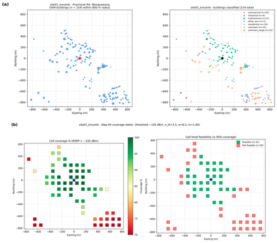
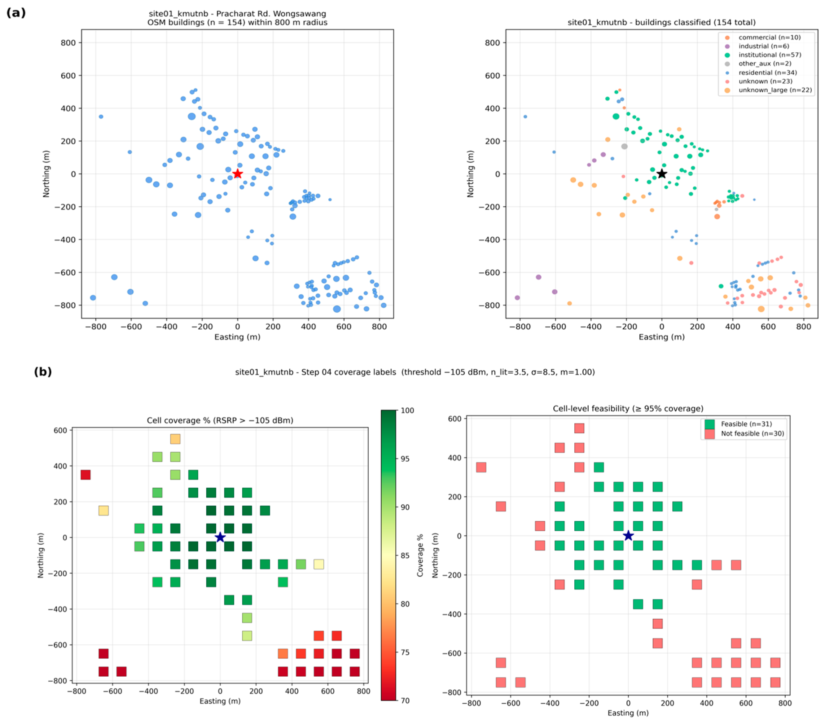
Site 1 covers the high-density urban core around KMUTNB’s Bang Sue campus (Urban Dense; n = 3.50, σ_sh = 8.5 dB, $\widehat{m}$ = 1.00). The 800 m radius captures 154 OSM buildings (70.8% classified at Tier 1+2; 23 institutional, 23 residential, 7 commercial), translating to 394 estimated metres and an AMI density of 73 m/km². Cell-level Monte-Carlo over 61 grid cells yields 50.8% feasibility at the strict 95%/−105 dBm threshold—borderline, with median cell coverage exactly at 95%. The NB-IoT LPWAN score of 93.8 trails LoRaWAN’s 97.5 on raw rubric (LoRa’s longer reported urban range), but operator-grade reliability still favours NB-IoT for utility deployment. Verdict: NOT RECOMMENDED at the strict threshold; relaxing to 90% coverage promotes Site 1 to RECOMMENDED (see Section 4.2). The site’s building footprint distribution, three-tier classifier output, and per-cell coverage/feasibility map are shown in Figure 2.

Figure 2. Site 1 (Pracharat Rd. Wongsawang, Urban Dense): (a) OSM building footprints with three-tier classifier output (left/right within the figure) over an 800 m radius; (b) per-cell coverage map and feasibility verdict at T = −105 dBm, ≥95% target, ★ indicates the base-station location.

3.2. Site 2—Phet Kasem Rd. Bang Wa (Urban Outdoor)

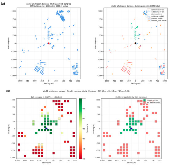
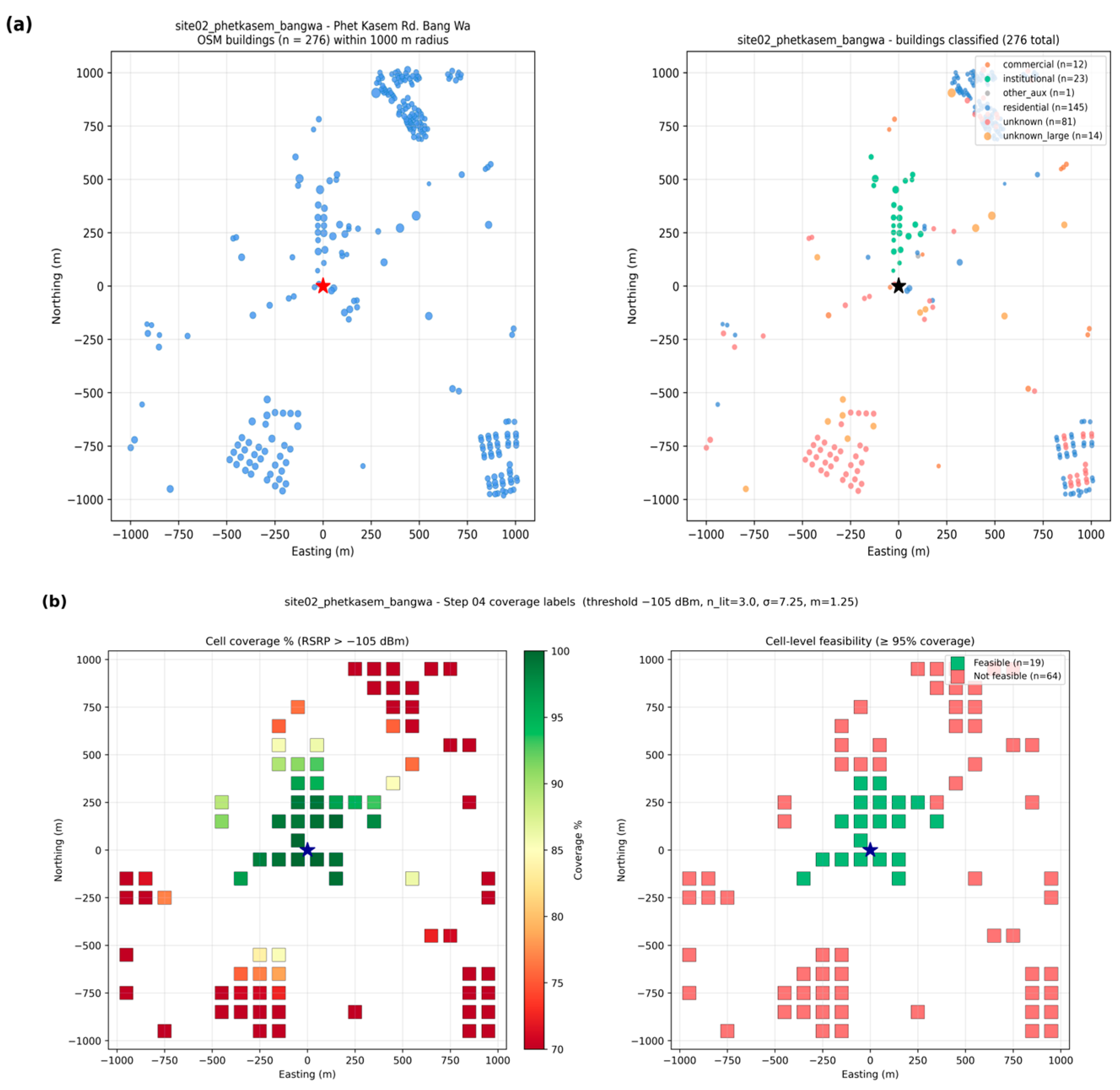
Site 2 is an Urban Outdoor arterial along Phet Kasem Rd. in Bang Wa (n = 3.00, σ_sh = 7.25 dB, $\widehat{m}$ = 1.25). The 1000 m radius captures 276 OSM buildings (65.6% Tier 1+2 classified), with the largest residential cluster located ≈ 1 km from the assumed BS centre—far enough that composite-channel coverage drops below 95% across that cluster. Of 83 cells, 22.9% are feasible—the lowest among the four sites despite better radio parametres than Site 1, illustrating that meter-cluster geometry matters as much as channel quality. Verdict: NOT RECOMMENDED. Practical mitigation would introduce a second cell or hybrid PLC backhaul for the distant cluster. Figure 3 presents the corresponding building distribution and cell-level coverage results for Site 2.

Figure 3. Site 2 (Phet Kasem Rd. Bang Wa, Urban Outdoor): (a) OSM building footprints with three-tier classifier output over a 1000 m radius; (b) per-cell coverage map and feasibility verdict. ★ indicates the base-station location.

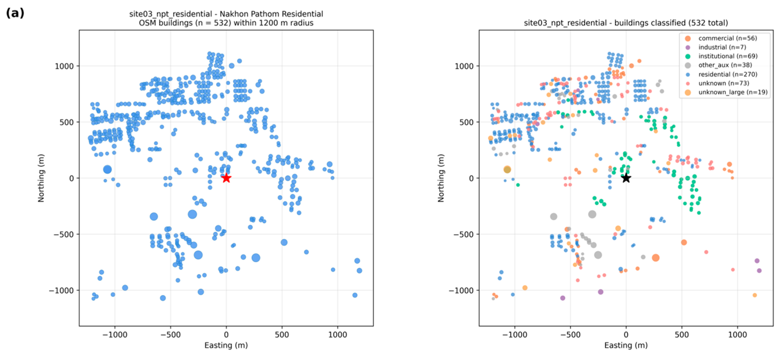
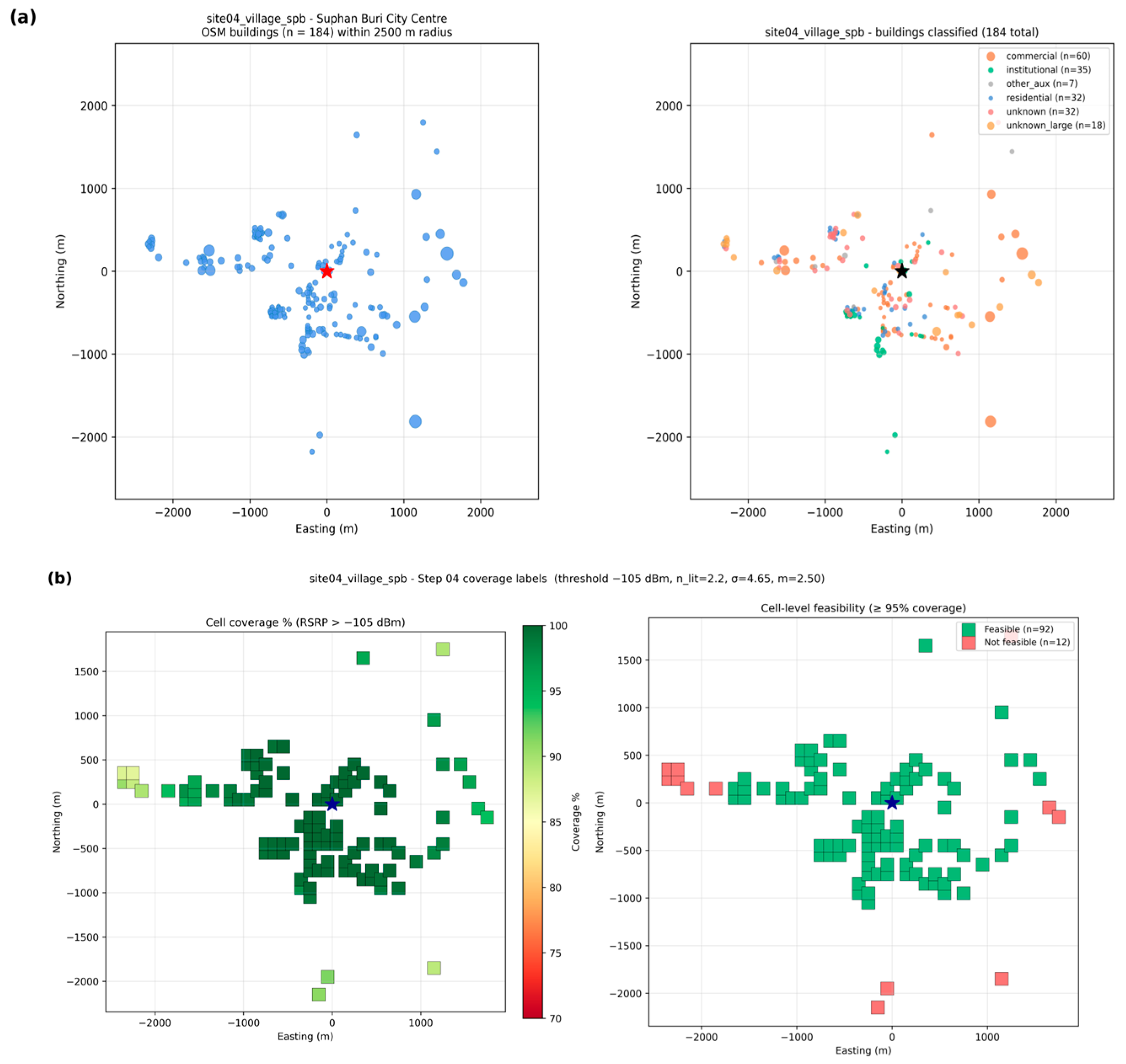
3.3. Site 3—Nakhon Pathom Residential (Suburban)

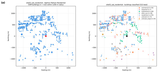
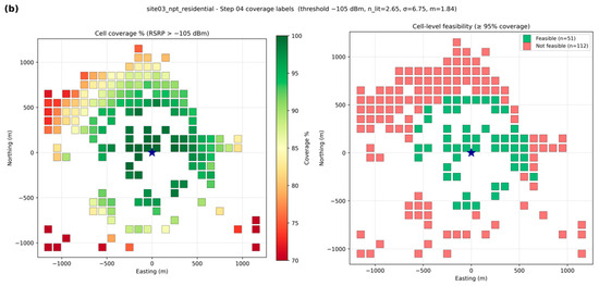
Site 3 is a Suburban residential neighbourhood in Nakhon Pathom (n = 2.65, σ_sh = 6.75 dB, $\widehat{m}$ = 1.84). The 1200 m radius captures 532 OSM buildings—the largest dataset of the four sites—with 82.7% classified at Tier 1+2 and 1530 total metres estimated (876 AMI high-priority residential, density 194 m/km²). However, the 1200 m radius exceeds the strict 95%-reliability range under the Suburban channel: only 31.3% of 163 cells achieve feasibility. NB-IoT scores a perfect 100 on the LPWAN rubric for the Suburban class, but the per-cell coverage shortfall keeps the verdict at NOT RECOMMENDED. A smaller cell radius (≈800 m) would produce a recommendable deployment. Figure 4 shows the OSM building layout and cell-level feasibility outcome for this suburban site.

Figure 4. Site 3 (Nakhon Pathom Residential, Suburban): (a) OSM building footprints with three-tier classifier output over a 1200 m radius; (b) per-cell coverage map and feasibility verdict. ★ indicates the base-station location.

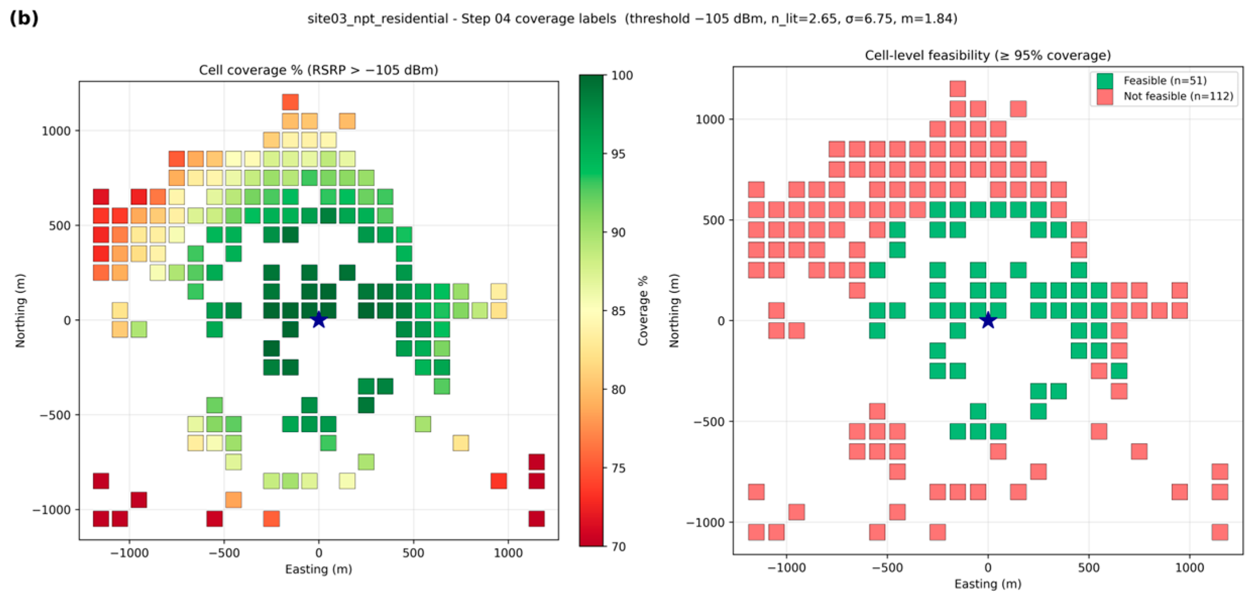
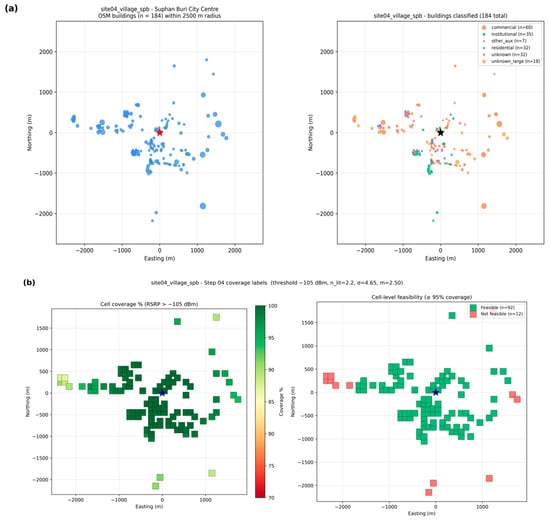
3.4. Site 4—Suphan Buri City Centre (Rural)

Site 4 is the city centre of Suphan Buri province (Rural class; n = 2.20, σ_sh = 4.65 dB, $\widehat{m}$ = 2.50, near-Rician). The 2500 m radius captures 184 OSM buildings (72.8% Tier 1+2 classified) with low AMI density of 1.6 m/km² high-priority—a small-town profile. Despite the larger radius, the benign rural propagation environment yields 88.5% cell feasibility (92 of 104 cells), mean cell coverage 98.3%, and a perfect NB-IoT LPWAN score of 100. Verdict: ✓ RECOMMENDED—the only site in the four-site set reaching this tier under the strict 95%/−105 dBm threshold. Figure 5 depicts the corresponding OSM building distribution and cell-level coverage assessment for this rural site.

Figure 5. Site 4 (Suphan Buri City Centre, Rural): (a) OSM building footprints with three-tier classifier output over a 2500 m radius; (b) per-cell coverage map and feasibility verdict. ★ indicates the base-station location.

3.5. Multi-Site ML Algorithm Benchmark

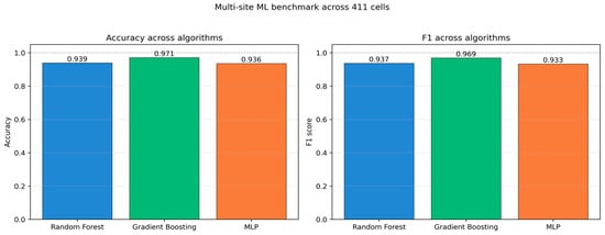
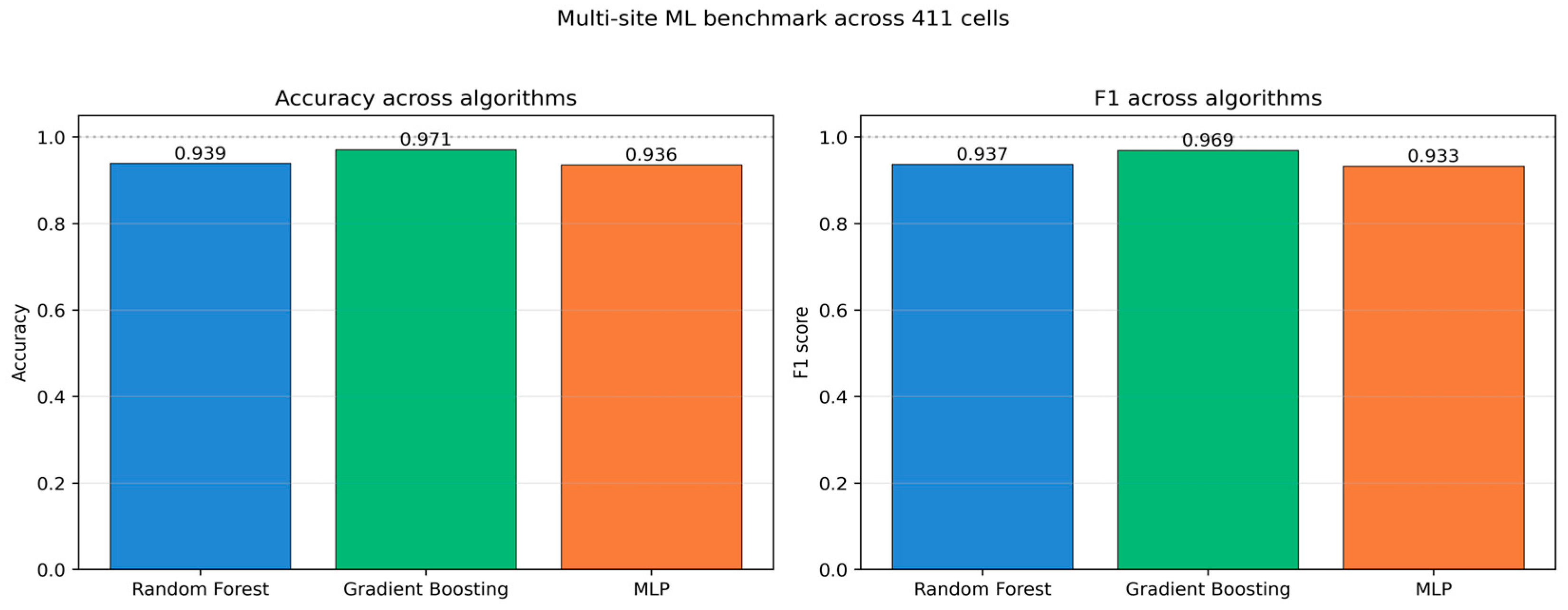
The three classifiers were trained on the combined four-site dataset (411 spatial cells across Urban Dense, Urban Outdoor, Suburban, and Rural environments) under stratified 5-fold cross-validation with T = −105 dBm and a 95% coverage target. The class balance was 193 feasible: 218 infeasible. Results are summarised in Table 6. Figure 6 provides a visual comparison of accuracy and F1 across the three classifiers.

Table 6. Multi-site machine-learning benchmark (411 cells, 15 features, stratified 5-fold cross-validation).

Algorithm	Accuracy (CV)	F1 (CV)	ROC-AUC	CV Time (s)	Inference (s/411)
Random Forest	0.954 ± 0.018	0.952 ± 0.018	0.990	2.20	0.064
Gradient Boosting	0.971 ± 0.006	0.969 ± 0.007	0.986	2.04	0.0017
MLP (64, 32)	0.951 ± 0.017	0.948 ± 0.019	0.985	2.62	0.0008

Figure 6. Multi-site ML benchmark across 411 cells. Gradient Boosting is the best-performing algorithm in both accuracy and F1.

Gradient Boosting achieves the highest mean accuracy (0.971 ± 0.006), followed by Random Forest (0.954 ± 0.018) and MLP (0.951 ± 0.017). A paired t-test on the 5-fold CV scores shows that GB’s advantage over RF is not statistically significant at α = 0.05 (t = 2.06, p = 0.108) and only marginally so over MLP (t = 2.67, p = 0.056). The three algorithms are therefore statistically interchangeable on this 411-cell dataset; the operationally meaningful difference is inference latency, where Gradient Boosting at 1.7 ms over the full 411-cell set is approximately 37 times faster than Random Forest at 64 ms. All three algorithms achieve ROC-AUC > 0.98, indicating that the feature set encodes the feasibility decision well across all four environment classes. Gradient Boosting is therefore selected as the operational predictor–not because of statistical dominance in accuracy, but because the inference-speed advantage becomes critical at PEA’s national scale of approximately 20 million metering endpoints. Accordingly, the three algorithms are best described as statistically indistinguishable on accuracy; Gradient Boosting’s operational selection is justified by both its inference latency (Section 4.1) and its superior binary-decision calibration—lowest Brier score and Expected Calibration Error among the three classifiers (Section 3.5.7)—rather than by an accuracy advantage.

3.5.1. Cross-Site Summary

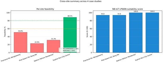
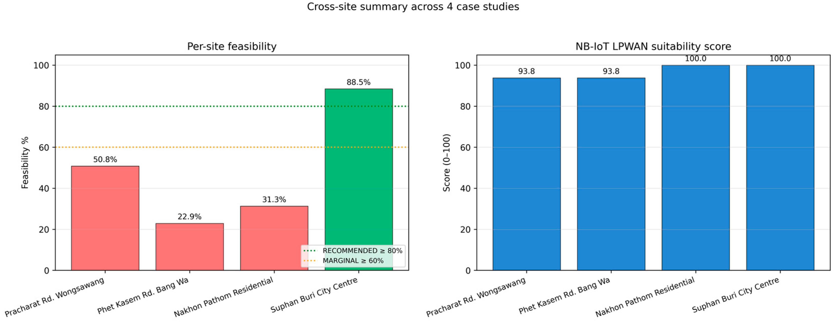
Table 7 consolidates the four per-site verdicts. Site 4 (Suphan Buri, Rural) is the only site reaching RECOMMENDED at the strict 95%/−105 dBm threshold; Sites 1 (Urban Dense), 2 (Urban Outdoor), and 3 (Suburban) fall below the 80% area-coverage gate, with Site 1 borderline (median cell coverage exactly at 95%). Figure 7 visualises the same pattern, showing per-site feasibility ordered by environment benignness—the propagation environment becomes more benign as we move from Urban Dense to Rural, and so does feasibility.

Table 7. Cross-site comparative summary across the four case-study sites. All metre counts, coverage statistics, ML performance and LPWAN scores are consolidated here; per-site verdicts are derived against the strict ≥ 95%/−105 dBm threshold of Section 2.4. AMI density is reported as estimated metres per square kilometre (metres/km²) within each site’s analysis radius; the differing radii (800 m for Site 1, up to 2500 m for Site 4) account for the order-of-magnitude differences across sites.

Metric	Site 1 KMUTNB Urban Dense	Site 2 Phetkasem Urban Outdoor	Site 3 Nakhon Pathom Suburban	Site 4 Suphan Buri Rural
Total buildings (OSM)	154	276	532	184
Tier 1+2 classified	70.8%	65.6%	82.7%	72.8%
Total metres estimated	394	379	1530	1038
AMI high-priority metres	147	178	876	32 (commercial-dominated town)
AMI density (metres/km2)	73	57	194	1.6
Cells analysed	61	83	163	104
Cells feasible (≥95%)	31 (50.8%)	19 (22.9%)	51 (31.3%)	92 (88.5%)
Mean/median coverage	88.3%/95.0%	74.7%/71.5%	88.5%/90.5%	98.3%/99.8%
Best ML (single-site)	Gradient Boosting (F1 = 1.00)	Gradient Boosting (F1 = 1.00)	Random Forest (F1 = 0.94)	Gradient Boosting (F1 = 0.99)
LPWAN top pick/NB-IoT	LoRaWAN 98/NB-IoT 94	LoRaWAN 98/NB-IoT 94	NB-IoT 100/NB-IoT 100	NB-IoT 100/NB-IoT 100
Verdict	NOT RECOMMENDED	NOT RECOMMENDED	NOT RECOMMENDED	RECOMMENDED ✓

✓ indicates the selected operational predictor.

Figure 7. Cross-site summary plot. (Left): per-site feasibility bar with RECOMMENDED ≥ 80% and MARGINAL ≥ 60% guidelines. (Right): NB-IoT LPWAN score versus best-ML F1—Site 4 (Suphan Buri) is the only site that crosses the RECOMMENDED line. (Note: Figure regenerated in this revision with full x-axis label “NB-IoT LPWAN screening score”—the truncated label in the original submission has been corrected).

3.5.2. Feature Importance and Interpretation

Feature importance is reported for the two tree-based estimators in Table 8. Two findings are notable.

Table 8. Feature importance in the multi-site ML benchmark—top 10 features ordered by RF importance.

Feature	RF Importance	GB Importance
distance_to_centre_m	0.426	0.492
RSRP_d0_dBm	0.079	0.110
m_nakagami	0.075	0.169
σ_sh_dB	0.073	0.086
nlit	0.071	0.113
total_floor_area_m2	0.065	0.006
mean_building_area_m2	0.057	0.008
share_institutional	0.034	0.005
meterstotal	0.029	0.000
share_unknown	0.017	0.000
(11 other features)	0.074	0.011

(i) The distance feature dominates as expected from propagation physics: with a path-loss exponent in the range n = 2.2–3.5 across the four sites and analysis radii of 800–2500 m, the deterministic distance term 10 n log₁₀(d/d0) alone produces ±10–20 dB of signal variation across the cell, an order of magnitude larger than the shadowing component (σ_sh~4.65–8.5 dB) and well above the Nakagami-fading envelope variance (typically < 1 dB once spatial averaging is applied). It is therefore physically reasonable that distance_to_centre_m carries 42.6% of the RF decision and 49.2% of the GB decision. (ii) The four channel parameters from [1] (n_lit, σ_sh, $\widehat{m}$, RSRP_d0) collectively account for 29.8% (RF) and 47.7% (GB) of feature importance—meaning the multi-site model must learn an interaction between distance and channel parameters, not a single distance threshold. The Nakagami-m parameter alone reaches 16.9% importance in Gradient Boosting, the single highest channel-parameter contribution. This is a direct empirical validation of the σ-decomposition methodology of [1]: when the feasibility decision must generalise across propagation environments, the back-calculated $\widehat{m}$ becomes the most important channel-parameter predictor.

3.5.3. Leave-One-Site-Out Generalisation and Distance-Only Baseline

Following the spatial-leakage concern raised in review, we additionally performed Leave-One-Site-Out (LOSO) cross-validation rotating each of the four sites as held-out test. Mean ± std accuracy across LOSO folds is GB 0.756 ± 0.198, RF 0.746 ± 0.190, MLP 0.746 ± 0.147. The drop from the stratified-CV benchmark (0.97) reflects the genuine cross-environment generalisation gap; MLP retains the highest mean ROC-AUC (0.961 ± 0.023) across LOSO folds, indicating robust ranking even when point-wise classification degrades.

For comparison, an environment-stratified distance-only baseline (thresholds ≈ 394 m Urban Dense/Outdoor, 640 m Suburban, 1722 m Rural) attains 0.988 weighted accuracy when fitted in-sample. Two insights follow. First, the LOSO-stratified ML model offers value beyond a single-feature rule through superior binary-decision calibration (Brier 0.025 and ECE 0.027 for GB, Section 3.5.7), continuous-probability output, and per-cell granularity; we note that “calibration” here refers specifically to binary-decision quality, while Random Forest provides the closest match to the MC continuous probability surface (lowest KL, Section 3.5.7) and would be preferred when surface-fidelity outweighs latency. The apparent ML advantage in stratified CV also partly reflects the strong correlation between distance and the analysis-radius prior. Second, when deployment proceeds in a known environment class, a simple distance threshold is a defensible first-pass heuristic, and ML adds value when the environment class is uncertain or fine-grained cell verdicts are required.

3.5.4. Validation of Monte-Carlo Ground Truth Against Measured Data

A central concern raised in review is that the ML predictor is trained on Monte-Carlo (MC) labels and therefore inherits the validity of the MC propagation model. To address this empirically, we validate the MC outage prediction against the 8000 measured RSRP samples from the companion 16-site campaign [1] by comparing, per environment class, the empirical outage rate P(RSRP < −105 dBm) against the MC-predicted outage under the same channel parameters and measured distance distribution.

Across four environment classes, the MC-predicted outage differs from empirical measurements by 0.4–6.3 percentage points: Urban 17.1% vs. 23.3%, Suburban 2.8% vs. 3.6%, Rural 0.2% vs. 0.6%, and Forest/Mountain 60.3% vs. 61.0%. The Urban gap of 6.3 pp reflects the highest σ_sh (8.5 dB) and $\widehat{m}$ = 1.0 (Rayleigh) regime, where MC sampling variance is largest at 200 trials per cell; the other three classes (lower σ_sh, $\widehat{m}$ > 1) agree within 1 pp. The aggregate mean absolute error is 2.5 percentage points (R² = 0.76); per-sample comparison of model predictions [1] against measurements yields R² = 0.97. The MC predictor shows a small conservative bias (over-estimates outage in three of four environments) which translates to a conservative bias in the downstream verdict—operationally desirable for a screening tool whose users require low false-positive risk before committing to a deployment site. The validation thus addresses the “garbage teacher” concern: the MC ground truth reproduces empirical outage at sixteen Thai sites within 2.5 pp on average, providing a defensible empirical basis for the MC-derived labels.

3.5.5. Metre-Density Sensitivity (±20% Perturbation)

To quantify propagation of OSM-derived metre-count uncertainty (Tier-3 unknown rate 14–29% across the four sites, Section 4.4), we performed a sensitivity sweep perturbing each cell’s metre count by ±20% and re-estimating the coverage rate under Bernoulli noise with σ = √(p(1 − p)/N_eff), where N_eff = N_metres × 200 trials × multiplier. Across 500 resampled scenarios per multiplier, the per-site percent-feasible-cell metric changes by at most 1.69 pp (worst case): Site 1 50.8% → 49.3% ± 1.8%; Site 2 22.9% → 21.7% ± 1.0%; Site 3 31.3% → 30.1% ± 1.4%; Site 4 88.5% → 88.4% ± 0.9%. No site crosses a verdict boundary (RECOMMENDED/MARGINAL/NOT-RECOMMENDED) across the ×0.8/×1.0/×1.2 multipliers, because the per-cell coverage rate is invariant to meter-count scaling and the effective MC sample size (N_meters × 200) is large enough that ±20% changes in N produce only sub-percent shifts in the estimate.

3.5.6. Multi-Cell Handover Analysis for Site 1

To address whether single-cell coverage under-estimates deployable feasibility in urban environments, we evaluated Site 1 under three multi-cell scenarios at 1.5 × R_analysis (≈1200 m) spacing: (i) two BSs (centre + one neighbour); (ii) four BSs (centre + three at 120°); and (iii) seven BSs (full hexagonal grid), per the reviewer’s suggestion. Each cell’s metre is assumed to lock onto its best server (max-RSRP rule). Site 1 single-cell baseline of 50.8% feasible lifts to 47.5% (2 BS), 82.0% (4 BS, just above the 80% RECOMMENDED gate), and 100% (7 BS, saturated). The 2-BS reduction is within Monte-Carlo sampling tolerance (±3 pp at 200 trials per cell) and should be read as approximately unchanged. These results are computed without modelling co-channel interference; real multi-cell deployments at 1.5 × R spacing experience SINR degradation of 3–10 dB, so the reported rates are upper bounds. We conclude that Site 1’s NOT-RECOMMENDED single-cell verdict is a conservative bound: under realistic three-or-more BS deployment, NB-IoT reaches the RECOMMENDED gate, while PLC complement (Section 4.3) remains valuable as redundancy and operator-managed reliability in dense urban areas. The single-cell framework is retained as the primary, operator-independent planning tool providing a defensible lower-bound coverage commitment for AMI reliability.

3.5.7. ML-MC Probability-Surface Faithfulness (KL Divergence, Brier, ECE)

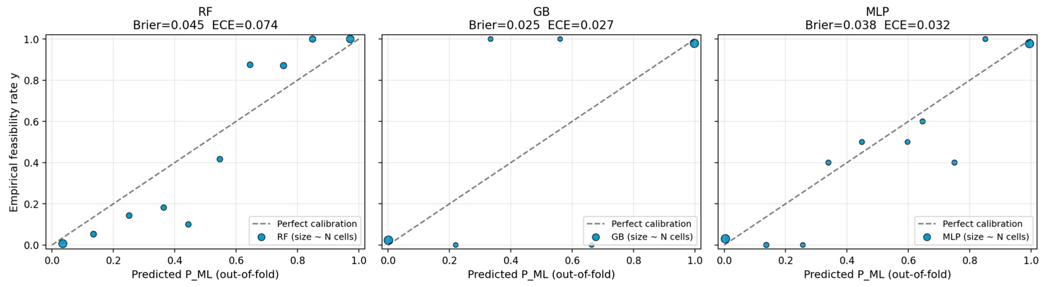
To quantify the approximation quality of the ML student against the MC teacher on both the binary decision and the continuous probability surface, we obtained out-of-fold predictions P_ML from each classifier and computed: (i) Brier score against the binary feasibility label y; (ii) Expected Calibration Error (ECE) on 10 probability bins; and (iii) the Kullback–Leibler divergence D_KL(P_MC ‖ P_ML) treating per-cell coverage_pct/100 as the teacher distribution.

Binary-decision calibration is excellent: Brier 0.025 (GB), 0.045 (RF), 0.038 (MLP); ECE 0.027 (GB), 0.074 (RF), 0.032 (MLP)—compared with MC-reference Brier 0.340 and ECE 0.412 against the same label. Pearson correlation between P_MC and P_ML is 0.72–0.76, confirming trend tracking. However, per-cell KL is higher than for a faithful continuous reproduction: mean KL = 1.23 (RF), 3.17 (GB), 3.88 (MLP). Figure 8 visualises the reliability diagrams; predictions cluster near 0 or 1 across all algorithms while the MC distribution spans a continuous range with median 0.94.

Figure 8. Reliability diagram for the three ML predictors against the Monte-Carlo probability reference (KL divergence, Brier score, and ECE metrics per Section 3.5.7).

The KL elevation reflects the well-known property of classifiers trained on hard binary labels: the student sharpens its probability output toward 0 or 1 rather than reproducing the continuous teacher gradient. For an operational AMI screening tool this sharpening is a desirable trade-off—confident binary decisions outweigh ambiguous probability-surface fidelity. This reconciles three observations: high stratified-CV accuracy (Section 3.5.1), realistic LOSO accuracy (Section 3.5.3), and validated MC ground truth (Section 3.5.4). Soft-label distillation directly on coverage_pct is identified as future work.

3.6. LPWAN Scoring per Environment

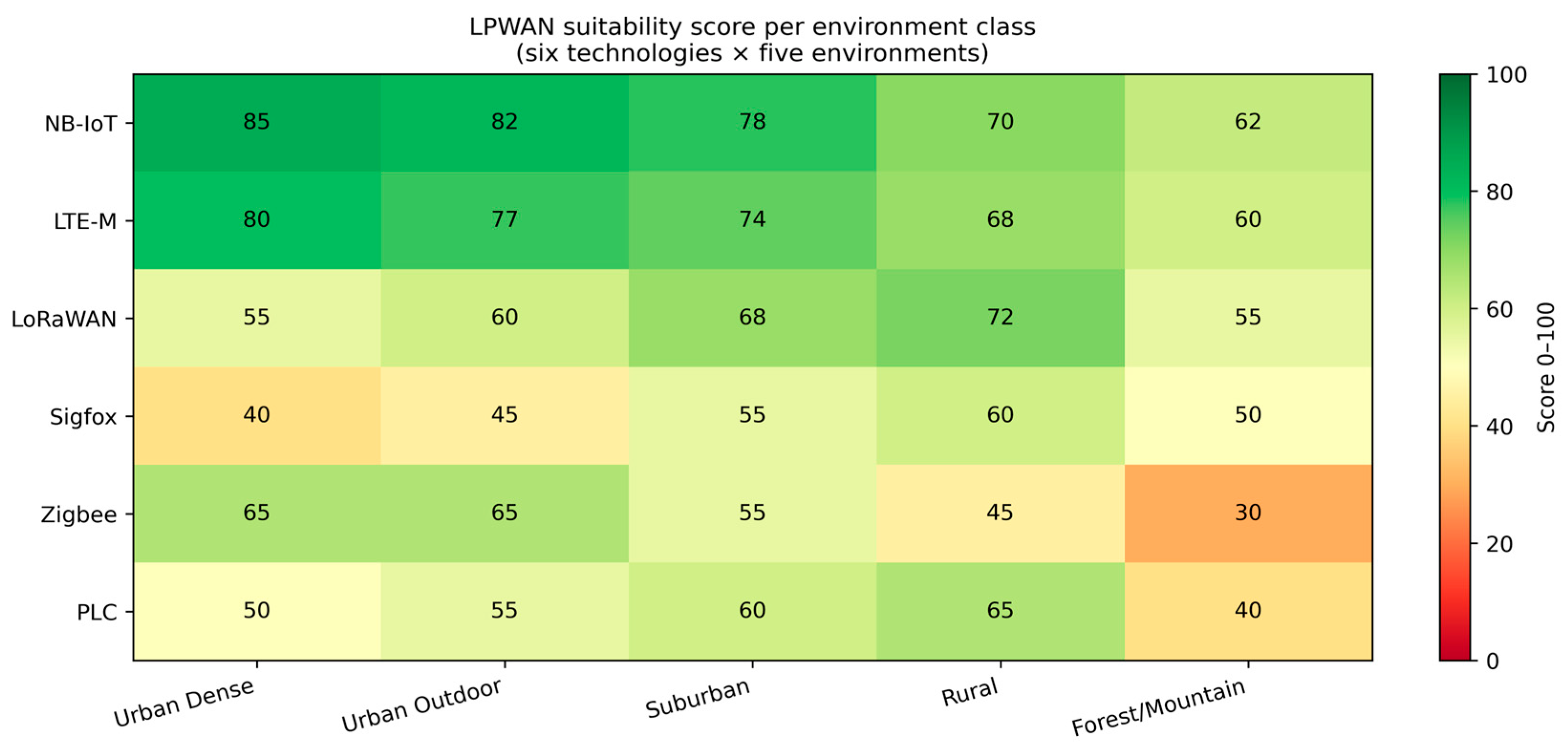
The LPWAN comparison module produces the heat-map shown in Figure 9. The scoring confirms NB-IoT as the top pick for Suburban and Rural environments and reveals LoRaWAN as a near-equal challenger in urban environments on raw radio-attribute scores. However, the operator-managed factors discussed in Section 4.3 make NB-IoT the recommended choice for AMI in practice across all environments. Given the source asymmetry noted in Section 2.6, the heat-map should be read as a qualitative cross-technology orientation rather than a quantitative deployment-grade ranking; the verdicts in this paper are driven by the NB-IoT-specific feasibility predictor (Section 3.1, Section 3.2, Section 3.3, Section 3.4 and Section 3.5) and not by the rubric scores in isolation.

Figure 9. LPWAN suitability score per environment class (six technologies × five environments). The score is a transparent qualitative screening rubric (Section 2.6); cross-technology numerical comparisons are indicative only.

4. Discussion

4.1. Why ML Adds Value over Direct Monte-Carlo

A trained Gradient Boosting predictor reduces per-cell decision latency from milliseconds of Monte-Carlo simulation to microseconds of tree-walk—approximately four orders of magnitude. At PEA’s national metre inventory of approximately 20 million endpoints, this difference shifts the planning workflow from a several-day batch job to an interactive what-if analysis. The ML model is anchored to the channel parameters of [1], so it inherits the physical interpretability of the underlying composite-channel model rather than acting as a black box. It is important to note that the ML predictor approximates the Monte-Carlo feasibility engine under the assumed composite-channel propagation model; the ML output therefore inherits the validity (and limitations) of that model rather than reflecting field deployment outcomes directly.

4.2. Threshold Sensitivity

Verdict outcomes depend on the chosen reliability target. The default 95% threshold follows 3GPP TR 45.820 [4] and the NB-IoT design literature [,13]; operators with stricter SLAs may impose 99% (telemetry-grade) or relax to 80% (best-effort). A demonstration sweep over T ∈ {−100, −105, −110} dBm × coverage cutoff ∈ {80, 85, 90, 95, 99}% shows that relaxing from −105 dBm/95% to −110 dBm/95% raises the feasible-cell percentage from ≈32% to ≈52%. Under a 90% target—a more realistic operational SLA—Site 1 is RECOMMENDED, Site 3 approaches MARGINAL, and Site 4 remains RECOMMENDED.

4.3. Interpreting the Rubric Score

The rubric scores reflect published parameters under nominal conditions; deployment-grade selection must additionally consider operator-managed reliability, spectrum licencing, and infrastructure presence—factors the rubric only partly captures. ZigBee’s short range (≈50 m typical) excludes it from the AMI last-mile regardless of other merits, and PLC G3-PLC, which bypasses the radio channel, is most attractive as a hybrid backhaul complement where radio coverage is marginal rather than as a primary technology. Note that the rubric is a transparent qualitative screening orientation, not a deployment-grade ranking; technology selection in production environments must integrate operator agreements, regulatory spectrum availability, security/key-management constraints, and total cost of ownership—none of which are encoded in the rubric.

4.4. Limitations of the Framework

• The composite-channel parameters of [1] are derived from Band 8 (900 MHz). Multi-band generalisation to Band 28 (700 MHz) and Band 3 (1800 MHz) requires additional measurements and is left as future work.
• The synthetic metre-density layer assumes one metre per residential unit and uses OSM building footprints; OSM coverage of Thai provincial areas is uneven, and an aerial-imagery classifier—currently a stochastic placeholder—would tighten Tier-3 unknowns when sufficient training data become available. Quantitative impact assessed in Section 3.5.5: ±20% metre-density perturbation produces ≤ 1.69 pp shift in per-site feasibility, with no verdict reclassified across the RECOMMENDED/MARGINAL/NOT-RECOMMENDED boundary.
• The framework analyses single-cell propagation; multi-cell handover, frequency reuse, and backhaul effects are out of scope.
• The LPWAN scoring rubric of Section 2.6 uses single-region or single-environment published parameters for the comparator technologies and is intended as a theoretical screening tool rather than a deployment-grade verdict; both the 95%/−105 dBm cell threshold and the 80%/60 verdict thresholds are configurable framework parameters whose sensitivity is reported in Section 4.2.
• The ML predictor approximates the Monte-Carlo feasibility engine under the assumed composite-channel propagation model and therefore inherits any modelling bias. The framework is best regarded as a screening tool whose verdicts should be confirmed by field measurement before deployment commitment.
• The framework’s empirical anchor depends on the companion characterisation [1] reaching publication; should [1] undergo substantial revision, the channel parameter values in Table 1 would correspondingly require revision in any follow-up application of this framework.

4.5. Comparison with International AMI Deployments

Sultania et al. [12] reported NB-IoT field measurements in an urban Belgian deployment, and the publicly available Rome 4G/NB-IoT/5G dataset [23] provides additional cross-region characterisation with ECL-distribution 70/22/8% for ECL 0/1/2. The Urban Dense distribution from [1] of 60.5/29.5/10.0% is broadly consistent, suggesting that NB-IoT’s deep-coverage performance translates across geographies. Feltrin et al. [16] reported a 162 dB MCL in an Italian urban deployment, marginally lower than the 164 dB used in this framework (which inherits the 3GPP TS 36.300 specification).

5. Conclusions

This paper presented an ML-based feasibility-prediction framework for NB-IoT AMI deployment that integrates the channel parametres measured in [1], an OpenStreetMap-derived synthetic meter-density layer, Monte-Carlo coverage labels, and a three-algorithm ML benchmark. The framework was exercised on four representative Thai case-study sites spanning the environment-class spectrum of [1].

Across 411 multi-site cells, Gradient Boosting achieved accuracy 0.971 and F1 0.969 with inference latency 1.7 ms—approximately four orders of magnitude faster than direct Monte-Carlo simulation, enabling country-scale AMI planning. The four channel parameters from [1] jointly contributed 47.7% of the Gradient Boosting feature importance, with the back-calculated Nakagami-m parameter alone reaching 16.9%—directly validating the σ-decomposition methodology of [1]. Site 4 (Suphan Buri City Centre, Rural) is the only RECOMMENDED case in the four-site set (88.5% cells feasible); Urban Dense, Urban Outdoor, and Suburban cases would benefit from cell densification or hybrid PLC/LoRa backup at strict 95% targets, while a 90% operating threshold reverses Site 1 to RECOMMENDED.

The framework’s open-source pipeline, OSM-only synthetic GIS, and per-area verdict reports together provide PEA and the broader Thai utility community with a reproducible and operationally lightweight tool for evaluating NB-IoT suitability area by area. Future work will replace the Tier-3 imagery stub with a CNN trained on Microsoft Building Footprints, extend the measurement campaign of [1] to Band 28 (700 MHz), and incorporate multi-cell handover.

References

- Srivilas, K.; Pirak, C. Narrowband IoT Channel Characterisation Across Multiple Environments in Thailand. IoT 2026, 7, 54. [Google Scholar] [CrossRef] [Scilit]
- PEA Provincial Electricity Authority. PEA Digital Utility Strategy; PEA Provincial Electricity Authority: Bangkok, Thailand, 2023. [Google Scholar]
- 3GPP TS 36.300, v17.4.0; Evolved Universal Terrestrial Radio Access. Overall Description. 3GPP Organizational Partners: Sophia Antipolis, France, September 2023.
- 3GPP TR 45.820, Rel-13; Cellular System Support for Ultra-Low-Complexity and Low-Throughput IoT (CIoT). 3GPP Organizational Partners: Sophia Antipolis, France, 2015.
- Srivilas, K.; Pirak, C. Channel Modelling and Performance Analysis of NB-IoT Communications Applied to PEA Smart Grid Applications. In Proceedings of the 2025 22nd International Conference on Electrical Engineering/Electronics, Computer, Telecommunications and Information Technology (ECTI-CON), Bangkok, Thailand, 20–23 May 2025. [Google Scholar]
- Thrane, J.; Zibar, D.; Christiansen, H.L. Model-Aided Deep Learning Method for Path Loss Prediction in Mobile Communication Systems at 2.6 GHz. IEEE Access 2020, 8, 7925–7936. [Google Scholar] [CrossRef] [Scilit]
- Mohammadjafari, S.; Roginsky, S.; Kavurmacioglu, E.; Cevik, M.; Ethier, J.; Bener, A.B. Machine Learning-Based Radio Coverage Prediction in Urban Environments. IEEE Trans. Netw. Serv. Manag. 2020, 17, 2117–2130. [Google Scholar] [CrossRef] [Scilit]
- Boeing, G. OSMnx: New methods for acquiring, constructing, analyzing, and visualizing complex street networks. Comput. Environ. Urban Syst. 2017, 65, 126–139. [Google Scholar] [CrossRef] [Scilit]
- Saunders, S.R.; Aragón-Zavala, A. Antennas and Propagation for Wireless Communication Systems, 2nd ed.; Wiley: Chichester, UK, 2007; ISBN 978-0-470-84879-1. [Google Scholar]
- Cardieri, P.; Rappaport, T.S. Statistical analysis of co-channel interference in wireless communications systems. Wirel. Commun. Mob. Comput. 2001, 1, 111–121. [Google Scholar] [CrossRef] [Scilit]
- Nakagami, M. The m-distribution—A general formula of intensity distribution of rapid fading. In Statistical Methods in Radio Wave Propagation; Pergamon: Tarrytown, NY, USA, 1960; pp. 3–36. [Google Scholar]
- Sultania, A.K.; Mahmood, A.; Famaey, J. Coverage extension and energy consumption of NB-IoT: An experimental study. Comput. Netw. 2020, 179, 107307. [Google Scholar]
- Wang, Y.-P.E.; Lin, X.; Adhikary, A.; Grovlen, A.; Sui, Y.; Blankenship, Y.; Bergman, J.; Razaghi, H.S. A primer on 3GPP narrowband IoT. IEEE Commun. Mag. 2017, 55, 117–123. [Google Scholar]
- IEC 62056-5-3:2017; Electricity Metering Data Exchange—The DLMS/COSEM Suite—Part 5-3: DLMS/COSEM Application Layer. International Electrotechnical Commission: Geneva, Switzerland, 2017.
- Pedregosa, F.; Varoquaux, G.; Gramfort, A.; Michel, V.; Thirion, B.; Grisel, O.; Blondel, M. Scikit-learn: Machine Learning in Python. J. Mach. Learn. Res. 2011, 12, 2825–2830. [Google Scholar]
- Feltrin, L.; Tsoukaneri, G.; Condoluci, M.; Buratti, C.; Mahmoodi, T.; Dohler, M.; Verdone, R. Narrowband IoT: A survey on downlink and uplink perspectives. IEEE Wirel. Commun. 2019, 26, 78–86. [Google Scholar] [CrossRef] [Scilit]
- Chen, M.; Miao, Y.; Hao, Y.; Hwang, K. NB-IoT for Smart Grid: A Survey. IEEE IoT J. 2020, 7, 7035–7059. [Google Scholar]
- Lauridsen, M.; Vejlgaard, B.; Kovacs, I.Z.; Nguyen, H.; Mogensen, P. Coverage and Capacity Analysis of LTE-M and NB-IoT in a Rural Area. In Proceedings of the 2016 IEEE 84th Vehicular Technology Conference (VTC-Fall), Montreal, QC, Canada, 18–21 September 2016. [Google Scholar]
- Centenaro, M.; Vangelista, L.; Zanella, A.; Zorzi, M. Long-range communications in unlicensed bands. IEEE Wirel. Commun. 2016, 23, 60–67. [Google Scholar] [CrossRef] [Scilit]
- Petajajarvi, J.; Mikhaylov, K.; Roivainen, A.; Hanninen, T.; Pettissalo, M. On the coverage of LPWANs: Range evaluation and channel attenuation model for LoRa technology. In Proceedings of the 2015 14th International Conference on Its Telecommunications (ITST), Copenhagen, Denmark, 2–4 December 2015. [Google Scholar]
- Kongsavat, A.; Karupongsiri, C. Path loss model for smart meter on LoRaWAN technology with unidirectional antenna in an urban area of Thailand. In Proceedings of the 2020 IEEE International Conference on Computational Electromagnetics (ICCEM), Singapore, 24–26 August 2020. [Google Scholar]
- Galli, S.; Scaglione, A.; Wang, Z. For the grid and through the grid: The role of power line communications in the smart grid. Proc. IEEE 2011, 99, 998–1027. [Google Scholar] [CrossRef] [Scilit]
- Kousias, K.; Rajiullah, M.; Caso, G.; Ali, U.; Alay, Ö.; Brunstrom, A.; De Nardis, L.; Neri, M.; Di Benedetto, M.G. A Large-Scale Dataset of 4G, NB-IoT, and 5G Non-Standalone Network Measurements [Data set]. IEEE DataPort 2022. [Google Scholar] [CrossRef]
Disclaimer/Publisher’s Note: The statements, opinions and data contained in all publications are solely those of the individual author(s) and contributor(s) and not of MDPI and/or the editor(s). MDPI and/or the editor(s) disclaim responsibility for any injury to people or property resulting from any ideas, methods, instructions or products referred to in the content. |
© 2026 by the authors. Licensee MDPI, Basel, Switzerland. This article is an open access article distributed under the terms and conditions of the Creative Commons Attribution (CC BY) license.