Solar Photovoltaic Maximum Power Point Tracking (MPPT): A Comparative Analysis of Incremental Conductance, Q-Learning, and Transformer Deep Learning for Performance Evaluation Under Standard and Dynamic Environmental Scenarios

Abstract

Maximum power point tracking (MPPT) is essential for photovoltaic (PV) efficiency under dynamic environments. This paper presents a comparative analysis of three MPPT algorithms: incremental conductance (INC), Q-Learning (QL) reinforcement learning, and Transformer-inspired Machine Learning (TML) applied to a photovoltaic (PV) array configured in a 1S×3P with a DC-DC boost converter designed for a 48 V DC output. Simulations were performed under four scenarios in MATLAB/Simulink: standard test conditions (STC), irradiance variation, temperature variation, and combined wide-range variations. At STC, all three exceed 99% tracking efficiency, with QL achieving the highest efficiency, 99.914%; TML having the best output voltage regulation (48.071 V); and INC converging fastest (5.4 ms). Under dynamic irradiance variations, QL attained the highest average tracking efficiency (91.85%) and average output power (481.4 W), whereas INC converged within 36.9 ms. Under temperature variations, TML achieved the highest average tracking efficiency (97.448%) and average power output (549.30 W), while INC maintained the fastest convergence rate (68.6 ms). With wide-range combined variation, QL achieves the highest average tracking efficiency (91.32%) and output power (469.9 W), outperforming TML (84.06%) and INC (57.39%) by 7.3 and 33.9 percentage points, respectively; INC converges fastest (33.1 ms) but delivers 64.1% less output power than QL. The simulation results demonstrate that artificial intelligence-driven algorithms can significantly improve maximum power point tracking (MPPT) under dynamic conditions. To establish real-world viability, future work requires hardware-in-the-loop (HIL) testing and experimental validation.

1. Introduction

The global shift towards pollution-free and environmentally friendly energy generation systems has made renewable energy a leading technology for power generation. The rapid growth in demand for renewable energy has led to increased deployment of photovoltaic (PV) systems [1].

According to an International Energy Agency (IEA) study, global renewable energy capacity grew by 50% in 2023 compared to 2022, reaching around 510 GW, with solar PV accounting for three-quarters of this capacity expansion [2]. However, variations in environmental conditions, particularly irradiance and temperature, significantly influence PV system performance. Fluctuations in these parameters cause continuous shifts in the maximum power point (MPP), defined as the operating point at which the PV system delivers maximum power. Consequently, maintaining maximum energy harvesting under varying environmental conditions remains a major challenge in PV system design [3]. Due to these complexities, operating the PV system at a fixed voltage or current does not guarantee the extraction of the maximum available power. To address these challenges, maximum power point tracking (MPPT) techniques are widely employed. MPPT algorithms continuously monitor the PV system output and adjust the operating point to locate and maintain the true maximum power point despite varying environmental conditions [4]. The MPPT control algorithm is typically integrated into the power converter control loop to maximize energy extraction from the PV array, thereby enhancing overall system efficiency, reliability, and operational lifespan. Several algorithms for MPPT have been proposed in the literature. Traditional methods such as Perturb and Observe (P&O) and incremental conductance (INC) remain widely adopted because of their simplicity and ease of implementation [5,6]. Comparative analyses indicate that P&O is more efficient at low irradiance and low temperatures, whereas INC is preferable for applications requiring higher precision and dynamic adaptability [7,8]. A review of 47 MPPT variants demonstrated that INC outperformed P&O by an average efficiency margin of 1.3% across 12 irradiance profiles [9]. Similarly, a survey of 19 MPPT algorithms established INC as the reference benchmark for dynamic tracking performance [10]. Despite their widespread use, both P&O and INC algorithms face challenges under large, rapid MPP voltage variation caused by abrupt irradiance or temperature changes. These sudden changes can lead to slow convergence and persistent steady-state oscillation [11,12]. Recent studies further emphasize that both methods suffer from oscillatory behavior and reduced convergence speed under rapidly changing environmental conditions, thereby motivating the development of enhanced and hybrid MPPT techniques [8,12,13,14]. Consequently, current research focuses on enhancing conventional MPPT methods through adaptive and hybrid approaches. Modified INC adaptations incorporating variable step sizes and predictive control mechanisms have been proposed to reduce oscillations and improve convergence speed [15,16]. Similarly, advanced INC-based methods using variable step-size incremental conductance (VSS-INC) focus on balancing tracking speed and accuracy while reducing drift problems in rapidly changing environments [17,18]. In addition to these methods, various computational approaches are employed to achieve MPPT in challenging dynamic environments [19]. Deep learning, optimization, and machine learning methods are gaining attention as alternatives that better adapt to changing weather conditions and complex operational environments. For example, artificial intelligence techniques such as fuzzy logic control and artificial neural networks (ANNs) address the limitations of conventional methods by handling the nonlinearity of PV systems without requiring precise mathematical models [20,21,22,23,24].

More advanced optimization-based techniques, such as Particle Swarm Optimization (PSO), Semi-Definite Programming (SDP) [25], and Genetic Algorithms (GAs), have been developed to address challenges in highly dynamic G-T environments. These methods can accurately track the MPP under rapid environmental changes; however, their high computational demands may limit their suitability for real-time embedded applications [26,27]. Consequently, recent research on maximum power point tracking (MPPT) has focused on hybrid and adaptive statistical modeling techniques. These methods leverage both conventional and advanced data-driven strategies to enhance convergence speed, minimize steady-state oscillations, and improve robustness in complex conditions, positioning hybrid and advanced computational approaches as leading solutions for next-generation photovoltaic (PV) systems [28,29]. Adaptive tracking techniques have demonstrated the capacity to adapt tracking behavior over time without requiring explicit system modeling [30]. This adaptive capability results in fewer iterations, reduced state ripples, and higher accuracy compared with traditional methods [31,32,33]. Furthermore, recent studies have explored advanced prediction and correlation-based control strategies that utilize temporal relationships among system variables to improve tracking efficiency and stability under transient conditions [34,35,36,37,38,39]. For example, temporal correlation-based forecasting methods have been successfully applied in microgrid load prediction [40], while enhanced feature extraction techniques have demonstrated improved prediction accuracy compared with conventional forecasting methods [41,42]. In addition, advanced long-sequence forecasting approaches have shown significant potential for real-time MPPT control applications [43].

Despite the increasing adoption of advanced techniques for maximum power point tracking (MPPT), systematic, quantitative comparisons between incremental conductance (INC), reinforcement learning (RL), and attention-based MPPT methods under identical dynamic operating conditions remain limited in the existing literature. The present work addresses this gap by implementing all three algorithms within a MATLAB/Simulink model subjected to an identical scenario test protocol.

The present work addresses this gap by implementing all three algorithms within a MATLAB/Simulink model subjected to an identical scenario test protocol.

The primary contributions of this paper are as follows:

i.  

Systematic four-scenario evaluation of three algorithm classes under identical configuration and performance metrics. No prior comparative study combines incremental conductance (INC), tabular Q-Learning, and Transformer–deep learning across standard test conditions (STC), irradiance-only variation (G = 600–1200 W/m²), temperature-only variation (T = 0–75 °C), and combined G-T variation under a single experimental protocol [3,4,11,12].

ii. 

A Transformer encoder utilizing multi-scale Fourier tokenization is introduced for Maximum Point Tracking (MPPT). The complement token T5 (complement, $1-V_n$) provides a 3.6-fold thermal signal range of raw $V_n$ over a 75 °C span, introducing a physics-informed inductive bias to the multi-head self-attention mechanism that is absent in prior MPPT designs.

iii.

Exact, analytically derived training label $D^{*}=1-{\displaystyle \frac{V_{mp}(G,T)}{V_{out,target}}}$. Unlike ANN-MPPT methods that use empirical or lossless-formula references, this work formulates and calibrates the training label to the measured no-load target voltage (49.07 V), accounting for resistive voltage drop under rated current. The resulting D* = 0.4640 differs from the commonly used lossless approximation, D = 0.4521, by 0.0119 duty-cycle units, which is statistically significant for voltage-sensitive DC loads.

iv.

An evidence-based, six-scenario algorithm selection guide and detailed novelty comparison tables are established to benchmark this work against four recent machine learning MPPT studies. Comprehensive numerical data spanning 15 tables and 44 waveforms are provided to ensure complete independent verification of all reported results.

The remainder of the paper is organized as follows. Section 2 describes the PV system and boost converter design. Section 3 presents the algorithm formulations. Section 4 details the simulation framework and metric. Section 5 reports and analyzes results for each scenario. Section 6 presents cross-scenario comparative analysis.

2. System Photovoltaic (PV) System Model and Boost Converter Design

2.1. Photovoltaic (PV) Configuration

The photovoltaic (PV) array is modeled using three Kyocera KC200GT modules (Kyocera Corporation, Kyoto, Japan) connected in parallel (1S×3P), yielding a total rated power of 600.43 W under standard test conditions (STC). The KC200GT modules are characterized using the standard single-diode equivalent circuit, expressed as [44,45]

$$I_{pv}=I_{ph}-I_0\left[exp\left({\displaystyle \frac{V_{pv}+I_{pv}{R}_s}{n{V}_T}}\right)-1\right]-{\displaystyle \frac{V_{pv}+I_{pv}{R}_s}{R_{sh}}}$$

(1)

where the symbols are defined as follows (Table 1):

Table 1. Single-diode model equation parameters.

Symbol	Definition	Unit
$I_{pv}$	PV array output current	A
$I_{ph}$	Photocurrent (proportional to irradiance G)	A
$I_0$	Diode reverse saturation current	A
$V_{pv}$	PV terminal voltage	V
$R_s$	Series resistance	Ω
$R_{sh}$	Shunt (parallel) resistance	Ω
$N$	Diode ideality factor	Dimensionless
$V_T$	Thermal voltage	V

The photocurrent is expressed as $I_{ph}=I_{sc}\left({\displaystyle \frac{G}{G_0}}\right)\left[1+K_I\left(T-25\right)\right]$, where $G_0$ = 1000 $\mathrm{W}/{\mathrm{m}}^2$ is the reference irradiance and $K_I=0.06\mathrm{A}/°\mathrm{C}$ is the temperature coefficient of short-circuit current obtained from the KC200GT (Kyocera Corporation, Kyoto, Japan) datasheet [46].

The thermal voltage of a PV cell is defined as [47,48]

$$V_T={\displaystyle \frac{K{T}_{op}}{q}}$$

(2)

where “K is the Boltzmann constant”, “$T_{op}$ is the operation temperature”, and “q is the electron charge”.

The electrical parameters of the Kyocera KC200GT module under standard test conditions (STC) are presented in Table 2.

Table 2. Electrical parameters of the Kyocera KC200GT at STC (G = 1000 $\mathrm{W}/{\mathrm{m}}^2$, T = 25 °C) [46].

Parameter	Symbol	Value	Unit	Source
Maximum power	$P_{max}$	200.143	W	[46]
MPP Voltage	$V_{mp}$	26.3	V	[46]
MPP Current	$I_{mp}$	7.61	A	[46]
Open-Circuit Voltage	$V_{oc}$	32.9	V	[46]
Short-Circuit Current	$I_{sc}$	8.21	A	[46]
Temperature Coefficient (Voc)	${\displaystyle \frac{{dV}_{oc}}{dt}}$	−0.355	V/°C	[46]
Temperature Coefficient (Isc)	${\displaystyle \frac{I_{sc}}{dt}}$	0.06	A/°C	[46]

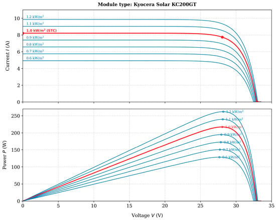
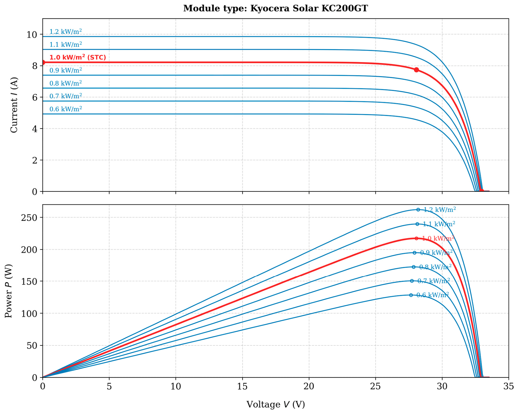
Figure 1 illustrates the current–voltage (I-V) and power–voltage (P-V) characteristic curves of the Kyocera KC200GT module under varying solar irradiance levels ranging from 0.6 $\mathrm{k}\mathrm{W}/{\mathrm{m}}^2$ to 1.2 $\mathrm{k}\mathrm{W}/{\mathrm{m}}^2$.

Figure 1. $\mathrm{I}-\mathrm{V}\mathrm{a}\mathrm{n}\mathrm{d}\mathrm{P}-\mathrm{V}$ characteristic curves under varying solar irradiance conditions. Scope note: All four simulation scenarios (S1–S4) in this paper test single-peak P-V characteristics under uniform irradiance across the array. Partial shading conditions, multi-peak P-V curve, and global MPPT are outside the scope of the study. The red line indicates the locus of maximum power points (MPP) across all irradiance levels, connecting the peak of each I-V and P-V curve to identify the optimal operating voltage for MPPT control at each irradiance condition.

2.2. Boost Converter Design and Output Voltage Target Derivation

The non-isolated DC–DC boost converter steps up the PV array voltage to the load bus. The no-load Simulink target output voltage is set to $V_{out,target}=49.07\mathrm{V}$ rather than a 48 V reference to ensure accurate calculation of duty-cycle values and evaluate MPPT performance.

2.2.1. Ideal Steady-State Conversion Ratio

For a lossless boost converter operating in continuous conduction mode, the ideal voltage conversion ratio is

$${\displaystyle \frac{V_{out}}{V_{in}}}={\displaystyle \frac{1}{1-D}}$$

(3a)

$$D=1-{\displaystyle \frac{V_{in}}{V_{out}}}$$

(3b)

At STC, $V_{in}$ =  $V_{mp}$ =  26.3 V. Setting $V_{out}$  =  48 V in the ideal equation gives the duty cycle

$$D_{ideal}=1-{\displaystyle \frac{26.3}{48}}=0.452$$

(4)

However, these neglect resistive losses in the inductor, MOSFET, and output capacitor.

2.2.2. Load Voltage Drop and No-Load Target Compensation

For a boost converter, the output voltage and load resistance are related by

$$R={\displaystyle \frac{V_{out}^2}{P_{out}}}$$

(5a)

where the $V_{out}$ is 48 V, and the power out is 600.43 W (3 × KC200GT at MPP):

$$R={\displaystyle \frac{{48}^2}{600}}=3.84\Omega$$

(5b)

$$I_{load}={\displaystyle \frac{V_{out}}{R}}$$

(6a)

$$={\displaystyle \frac{48}{3.84}}=12.5\mathrm{A}$$

(6b)

For a resistive load ($R_{load}$) of 3.84 Ω, the nominal rated output voltage is 48 V. However, the simulated output voltage under no-load conditions, $V_{out,NL}$ is 46.93 V rather than 48 V. This reduction is attributed to voltage drops across the boost converter components, including the inductor winding resistance, MOSFET on-state resistance, and diode forward voltage drop. Considering the inductor winding resistance $R_L$ and the MOSFET on-state resistance $R_{DS}$, actual output voltage under load is given by

$$R={\displaystyle \frac{V_{measured}^2}{P_{out}}}$$

(7)

$$R={\displaystyle \frac{{46.3}^2}{600}}={\displaystyle \frac{2143.69}{600}}=3.57\Omega$$

To get exactly 48 V at the output, back-calculate the required R; target $V_{out}$ is 48 V; the measured $V_{out}$ is 46.93 V.

$$Ratio={\displaystyle \frac{48}{46.3}}=1.0367$$

$$R_{new}=R_{old}\ast {\left({\displaystyle \frac{48}{46.3}}\right)}^2=3.84\ast {\left({\displaystyle \frac{48}{46.3}}\right)}^2=4.02\Omega$$

$$\approx 4.1\Omega \left(\mathrm{n}\mathrm{e}\mathrm{a}\mathrm{r}\mathrm{e}\mathrm{s}\mathrm{t}\mathrm{s}\mathrm{t}\mathrm{a}\mathrm{n}\mathrm{d}\mathrm{a}\mathrm{r}\mathrm{d}\mathrm{v}\mathrm{a}\mathrm{l}\mathrm{u}\mathrm{e}\right)\Omega$$

The no-load target voltage is established at $V_{out,target}=49.07\mathrm{V}$ to compensate for converter losses. The value 49.07 V is the iteratively calibrated Simulink set-point, obtained by adjusting the no-load output voltage until the measured resistive load output reached 48 V at D_mpp = 0.4640. This iterative process yielded the calibrated no-load target set-point $V_{out,target}$. Therefore, the theoretical duty cycle under standard test conditions is expressed as

$$D_{mpp}=1-{\displaystyle \frac{V_{mp}}{V_{out,target}}}=1-{\displaystyle \frac{26.3}{49.07}}=0.4640$$

(8)

Consequently, the calibrated value of D = 0.4640, rather than the idealized value of D = 0.4521, serves as the correct reference for evaluating the maximum power point tracking (MPPT) duty cycle, as it accurately accounts for the internal resistive voltage drop of the converter.

2.2.3. Boost Converter

In photovoltaic (PV) systems, a DC–DC boost converter operating at a fixed switching frequency is utilized to optimize energy extraction via maximum power point tracking (MPPT). By continuously adjusting the duty cycle, the converter regulates the PV array’s operating point to match the source and load impedances, thereby maximizing power transfer [49]. The mathematical formulation for the boost converter parameter design is expressed as follows:

i.  

Input capacitor sizing:

$$C_{in}={\displaystyle \frac{I_{pv}\ast D}{f_s∆V_{pv}}}$$

(9)

ii. 

Inductor design:

$$L={\displaystyle \frac{V_{in}D}{∆I{f}_s}}$$

(10)

iii.

Output capacitor:

$$C_{out}={\displaystyle \frac{I_{o}D}{f_s∆V_o}}$$

(11)

The inductor (L) is 150 $\mathsf{\mu }$H to handle 22.83 A without saturation. $C_{in}$ is 110 µF to stabilize $V_{pv}$ and reduces PV ripple,$C_{out}$ is 680 µF for a smooth 48 V output, $f_s$ is 20 kHz for the PWM Generator carrier frequency and interfaces the string with a 48 V. The boost voltage relationship is $V_{out}={\displaystyle \frac{V_{in}}{\left(1-D\right)}}$, where D ∈ [0.1, 0.9] is the MPPT-generated duty cycle [50].

3. MPPT Algorithms Formulation

3.1. Incremental Conductance (INC) Algorithm

The incremental conductance (INC) algorithm locates the maximum power point (MPP) by evaluating the derivative of PV power with respect to voltage [51,52,53]. At the MPP, ${\displaystyle \frac{dP}{dV}}=0$; to its left ${\displaystyle \frac{dP}{dV}}>0$; to its right ${\displaystyle \frac{dP}{dV}}<0$. Expanding through the product rule,

$$P=I\ast V$$

(12)

Differentiating with respect to the voltage, Equation (12) becomes

$${\displaystyle \frac{dP}{dV}}=I+V\ast \left({\displaystyle \frac{dI}{dV}}\right)=0\hspace{1em}\hspace{1em}\left(atMPPcondition\right)$$

(13a)

Rearranged MPP condition:

$${\displaystyle \frac{dI}{dV}}=-{\displaystyle \frac{I}{V}}$$

(13b)

In discrete-time implementation with sampling period $T_s$, the continuous derivative is approximated by finite difference:

$$∆V\left(k\right)=V_{pv}\left(k\right)-V_{pv}\left(k-1\right),\hspace{1em}\hspace{1em}∆I\left(k\right)=I_{pv}\left(k\right)-I_{pv}\left(k-1\right)$$

(14)

$${\displaystyle \frac{∆I\left(k\right)}{∆V\left(k\right)}}\approx {\displaystyle \frac{dI}{dV}}\hspace{1em}\mathrm{w}\mathrm{h}\mathrm{e}\mathrm{n}∆V\left(k\right)\ne 0$$

(15)

where $∆V\left(k\right)$ and $∆I\left(k\right)$ are the voltage and current increments at sample $k$. The MPPT condition is therefore evaluated through each of the following three-branch decisions [52,53,54]:

• If $∆V\left(k\right)=0$ and $∆I\left(k\right)=0$: $D\left(k+1\right)=D\left(k\right)$ [at MPP, hold]
• If $∆V\left(k\right)=0$ and $∆I\left(k\right)>0$: $D\left(k+1\right)=D\left(k\right)+∆D$ [increase $V_{pv}$]
• If $∆V\left(k\right)\ne 0$: compare ${\displaystyle \frac{∆I\left(k\right)}{∆V\left(k\right)}}$ with ${\displaystyle \frac{-I\left(k\right)}{V\left(k\right)}}$

  ○ 

  If ${\displaystyle \frac{∆I\left(k\right)}{∆V\left(k\right)}}>-{\displaystyle \frac{I\left(k\right)}{V\left(k\right)}}$: $D\left(k+1\right)=D\left(k\right)+∆D$ [left of MPP]

  ○ 

  If ${\displaystyle \frac{∆I\left(k\right)}{∆V\left(k\right)}}=-{\displaystyle \frac{I\left(k\right)}{V\left(k\right)}}$: $D\left(k+1\right)=D\left(k\right)$ [exact MPP or at MPP]

  ○ 

  If ${\displaystyle \frac{∆I\left(k\right)}{∆V\left(k\right)}}<-{\displaystyle \frac{I\left(k\right)}{V\left(k\right)}}$: $D\left(k+1\right)=D\left(k\right)-∆D$ [right of MPP]

$$D\left(k+1\right)=D\left(k\right)\pm ∆D,D\left(k\right)\in \left[D_{min},D_{max}\right]=\left[\mathrm{0.10,0.90}\right]$$

(16)

where ΔD is a fixed perturbation step applied at 2 kHz. The minimum measurable $V_{pv}$ shift per cycle is $∆V_{min}\approx 0.16\mathrm{V}$. For MPP displacements exceeding ${\displaystyle \frac{∆V_{min}}{D}}$ cycles (e.g., $\ge 3\mathrm{V}$ at T = 0 °C requiring $\ge$ 31 steps $\approx 15.5\mathrm{m}\mathrm{s}$), convergence may be incomplete within the phase window under the combined transition, which constitutes a structural coverage failure inherent to fixed-step INC [55,56].

3.2. Q-Learning Reinforcement Learning

Reinforcement learning-based maximum power point tracking (MPPT) optimizes power as a sequential decision-making task using a Markov Decision Process (MDP) [57,58].

The MDP five-tuple is defined as

$$MDP=\left(S,A,R,\gamma ,\alpha \right)$$

(17)

where S is the finite set of observable system states; A is the finite action set available to the agent; R is the reward function (change in $P_{pv}$); γ = 0.90 is the discount factor; and α = 0.10 is the learning rate. The QL agent operates at a 500 µs sampling interval and updates the action-value function via the Bellman temporal-difference rule. For Scenarios S1 and S3, the state space uses a three-sample power-change history (27 states). For Scenario S2, the Q-table is trained over G = 600–1200 W/m² at T = 25 °C, preserving the 27-state representation. For Scenario S4 (G = 600–1200 W/m², T = 0–75 °C), the state space is extended with an explicit temperature bin, as described in Section 3.2.1.

3.2.1. State and Reward Formulations

For Scenarios S1–S3, the state $s_t$ is a three-sample temporal window encoding the sign of the power change:

$$s\left(t\right)=\left(sgn\left(∆P_t\right),sgn\left(∆P_{t-1}\right),sgn\left(∆P_{2-1}\right)\right)$$

(18)

yielding $\left|\mathcal{S}\right|=3^3=27$ discrete states. For Scenario S2, the Q-table is retrained on a uniform irradiance grid G ∈ {600, 625, …, 1200} W/m² at T = 25 °C (25 irradiance levels) using this same 27-state representation.

Extension for Scenario S4. Under combined G–T variation, identical-sign triples can arise at operating points that require different duty cycles as temperature varies. To resolve this, the S4 state space is extended:

$$s_t=\left(V_{bin},{∆P}_{bin},T_{bin}\right)$$

(19)

where $V_{bin}\in \left\{1,\dots \dots ,20\right\}$ discretizes $V_{pv}$ over $\left[\mathrm{10,32}\right]V$; $∆P_{in}\in \left\{1,\dots \dots ,5\right\}$ classifies the power increment into five levels; and $T_{bin}\in \left\{1,\dots \dots ,6\right\}$ maps temperature to six bands: [0–10), [10–25), [25–35), [35–50), [50–62), [62–75] $°\mathrm{C}$. The resulting Q-table has $20\ast 5\ast 6\ast 3=1800\mathrm{e}\mathrm{n}\mathrm{t}\mathrm{r}\mathrm{i}\mathrm{e}\mathrm{s}.$ The reward function for all scenarios is

$$R_t=P_{pv,t}-P_{pv,t-1}$$

(20)

Using $∆P_{pv}$ rather than absolute power, the reward remains irradiance-independent and transferable across all G–T operating conditions.

3.2.2. Action Space and Duty-Cycle Modulation

The action space is $A=\left\{-∆D,0,+∆D\right\}$. For Scenarios S1–S3, the step size is set to $∆D=0.003$, consistent with the baseline controller. For Scenario S4, a temperature-adaptive step size is employed as follows:

$$∆D=0.003+0.001·min\left({\displaystyle \frac{\left|T-25\right|}{50}},1\right)$$

(21a)

This formulation accounts for the wider optimal duty-cycle range of [0.4014, 0.5894] required across 0–75 °C, compared to [0.4390, 0.5142] for S3. Consequently, the perturbation step size increases from $∆D=0.003$ under standard test conditions (STC) to $∆D=0.004$ at extreme temperatures. At each sampling interval of 500 μs, the duty cycle is constrained within the range $D\in \left[\mathrm{0.10,0.90}\right]$ to ensure stable converter operation and prevent saturation.

3.2.3. Q-Table Update and Convergence

The action-value function $Q(s,a)$ is updated at each sampling instant via Bellman temporal-difference rule:

$$Q\left(s_t,a_t\right)\leftarrow Q\left(s_t,a_t\right)+\alpha \left[r_t+\gamma \underset{a}{\max }Q(S_{t+1},a)-Q(s_t,a_t)\right]$$

(21b)

with a learning rate $\alpha =0.10$ and discount factor $\gamma =0.90$. For Scenarios S1–S3, the $27\ast 3$ Q-table is initialized with zero values and updated through an $\epsilon$-greedy exploration strategy, where $\epsilon$ decays from 1.0 to 0.05 over 600 episodes. For Scenario S4, a 20 × 5 × 6 × 3 Q-table is pre-seeded with physics-derived initial values to reduce the computational and exploration burden. During the simulation, the controller selects the greedy action $\underset{a}{\max }Q(S_{t+1},a)$. Online Bellman updates continue during the S4 simulation, enabling adaptive corrections as the system encounters new (G, T) operating points. The configuration parameters for both operating modes are summarized in Table 3B.

Table 3. (A) DC–DC boost converter parameters and no-load voltage target derivation. (B) Summarizes the QL configuration for both modes. (C) Parameters of configuration for scenarios.

(A)
Parameter	Symbol	Value	Unit
Capacitor	$C_{in}$	110	µF
Inductor	$L$	150	µH
Input Capacitor	$C_{out}$	680	µF
Load Resistance	$R_L$	4.1	Ω
Switching Frequency	$f_s$	20	kHz
Target Load Voltage	$V_{out,load}$	48.0	V
Calibrated No-Load Target	$V_{out,target}$	49.07	V
STC Optimal Duty Cycle	$D_{mpp}$	0.4640	—
Rated Output Current at 48V	$I_{out}$	11.71	A
(B)
Parameter	S1–S3		S4
State representation	27 states (sign history)		20 × 5 × 6 = 600 state cells
Q-table size	27 × 3 = 81 entries		20 × 5 × 6 × 3 = 1800 entries
Initialization	Zero		Analytical D*(T) pre-seed
Temperature in state	No		Yes, $T_{bin}$ (6 bands, 0–75 °C)
Step size $∆D$	0.003 (fixed)		0.003–0.004 (T-adaptive, Equation (21))
Learning rate α	0.10		0.10
Discount factor γ	0.90		0.90
ε-greedy training	Yes		Pre-seeded
(C)
Parameters	S1–S3 (6-Token)		S4 (7-Token)
Tokens L	6		7 (adds T7 thermal)
Training samples N	650 $\left(G\ast Tgrid\right)$		400 $(25\ast 16grid)$
Optimizer/$I_r$	Adam/$\alpha =3\ast {10}^{-3}$		Adam/$\alpha =3\ast {10}^{-4}$
Stopping criterion	Early stopping (patience = 60)		5000 epochs, batch = 32
Training RMSE	0.000363		0.000218
Validation RMSE	0.000418		0.000176
Val/Train ratio	1.15		0.807
$D_{lo}/D_{hi}$	0.3916/0.6036		0.3514/0.6394
Parameters	9889		4585

Note: ${\mathrm{V}}_{\mathrm{o}\mathrm{u}\mathrm{t},\mathrm{t}\mathrm{a}\mathrm{r}\mathrm{g}\mathrm{e}\mathrm{t}}$ = 49.07 V is the no-load Simulink set-point, not 48 V. The resistive load drop accounts for the 1.07 V difference. ${\mathrm{R}}_{\mathrm{L}}$ = 4.1 Ω is the calibrated load resistance (${\mathrm{R}}_{\mathrm{c}\mathrm{a}\mathrm{l}\mathrm{i}\mathrm{b}\mathrm{r}\mathrm{a}\mathrm{t}\mathrm{e}\mathrm{d}}={\mathrm{R}}_{\mathrm{i}\mathrm{d}\mathrm{e}\mathrm{a}\mathrm{l}}\mathrm{\ast }{\left({\displaystyle \raisebox{1ex}{$48$}\!\left/ \!\raisebox{-1ex}{$46.93$}\right.}\right)}^2\approx 4.02\Omega$, rounded to the nearest standard simulation value of 4.1 Ω); the ideal lossless design value ${\mathrm{R}}_{\mathrm{i}\mathrm{d}\mathrm{e}\mathrm{a}\mathrm{l}}$ = 3.84 Ω appears in Equation (5b) and is distinct. Rated output current ${\mathrm{I}}_{\mathrm{o}\mathrm{u}\mathrm{t}}={\displaystyle \raisebox{1ex}{$48$}\!\left/ \!\raisebox{-1ex}{$4.1$}\right.}=11.71\mathrm{A}$, ${\mathrm{D}}_{\mathrm{m}\mathrm{p}\mathrm{p}}$ = 0.4640 is derived from Equation (8) using ${\mathrm{V}}_{\mathrm{o}\mathrm{u}\mathrm{t},\mathrm{t}\mathrm{a}\mathrm{r}\mathrm{g}\mathrm{e}\mathrm{t}}$.

3.3. Transformer-Inspired Machine Learning Model (TML)

The TML utilizes a Transformer encoder architecture to directly map normalized inputs (PV terminal voltage and current) to the optimal duty cycle (D), without the need for iterative perturbation, as the model’s self-attention mechanism captures complex dependencies to determine the duty cycle directly. The multi-head self-attention (MHSA) mechanism captures cross-variable dependencies between the electrical operating point and the ambient conditions, enabling single-step duty-cycle calculation at a 2 kHz maximum power point tracking (MPPT) update rate. For Scenarios S1–S3, the encoder operates on a six-element Fourier feature sequence (L = 6). For Scenario S4 (G = 600–1200 $\mathrm{W}/{\mathrm{m}}^2$, T = 0–75 °C), a seventh thermal input feature is appended (L = 7), providing the attention mechanism with a direct temperature signal that resolves the $G-T$ degeneracy inherent in the six-element representation.

3.3.1. Multi-Scale Feature Tokenization

The inputs are normalized as $V_n={\displaystyle \frac{V_{pv}}{32.9}}$ and $I_n={\displaystyle \frac{I_{pv}}{24.63}}$, where ($V_n$, $I_n\in$ [0,1]). For Scenario S4, the temperature is normalized as $T_n={\displaystyle \raisebox{1ex}{$T$}\!\left/ \!\raisebox{-1ex}{$75$}\right.}$. The input matrix $\tau ϵ{\mathbb{R}}^{L\ast 4}$ contains.

L = 6 feature vectors for Scenarios S1–S3 and L = 7 feature vectors for Scenario S4 are defined as follows:

i.  

TI (Polynomial): Captures raw magnitudes $\left[V_n,I_n,V_n^2,I_n^2\right]$.

ii. 

T2 (Cross product): Power-related $\left[V_n{I}_n,\left|V_n-I_n\right|,{\displaystyle \frac{V_n+I_n}{2}},V_n(1-I_n)\right]$.

iii.

T3 and T4: Fourier expansion at $\pi$ and $2\pi$ frequencies, specifically ${\displaystyle \frac{1}{2}}\sin \left(k\pi x\right)+{\displaystyle \frac{1}{2}}$, to capture periodic non-linearities.

iv.

T5 (complement): Contains $\left(1-V_n\right)$ and $\left(1-I_n\right)$ terms. This token is a critical temperature indicator; $\left(1-V_n\right)$ shift by $3.6$ times more than raw $V_n$ across a temperature $0-75°\mathrm{C}$ range, aiding thermal sensitivity.

v. 

T6 (Cubic): High-order interaction like $V_n^2(1-I_n)$ for fine-grained boundary detection.

vi.

T7 (Thermal vector, Scenario S4 only): $[T_n,1-T_n,T_n^2,{\left(1-T_n\right)}^2]$, a direct temperature signal that resolves the irradiance–temperature (G-T) degeneracy, where identical ${(V}_n{,I}_n)$ operating pairs can arise at different (G-T) combinations and require distinct optimal duty cycles $\left(D^{*}\right)$.

3.3.2. Transformer Architecture Formulation

The token sequence $\tau$ is mapped into a $d_{model}=24$ dimensional latent subspace via a transformation matrix $W_eϵ{\mathbb{R}}^{2\ast 24}$ with a fixed positional encoding matrix $\mathsf{{\rm P}}ϵ{\mathbb{R}}^{2\ast 24}$:

$$Z_0=\tau W_e+\mathsf{{\rm P}}$$

(22a)

The mapped matrix passes through two stacked structural encoder layers, each comprising the following:

i. 

A multi-head self-attention (MHSA) ($h=4heads$ and a scaling factor of $\sqrt{d_k}=\sqrt{6}$) utilizing scaled dot-product formulation:

$$Attention\left(Q,K,V\right)=softmax\left({\displaystyle \frac{Q{K}^T}{\sqrt{d_k}}}\right)V$$

(22b)

This is followed by a position-wise feed-forward network (FFN) with a hidden dimension $d_{ff}=48$ and ReLU activation.

ii.

Residual connections with layer normalization.

The final layer matrix $H_Bϵ{\mathbb{R}}^{L\ast 24}$ is compressed via global average pooling to a $1\ast 24$ state vector. A sigmoid-activated linear combination stage yields the optimal duty-cycle calculation:

$$D^{*}=D_{lo}+\sigma \left(pool\left(H_B\right)·W_o+b\right)·\left(D_{hi}-D_{lo}\right)$$

(22c)

For Scenarios S1–S3, the operational bounds are set to $D_{lo}=0.3916,D_{hi}=0.6036$. For Scenario S4, the bounds are extended to $D_{lo}=0.3514,D_{hi}=0.6394$, thereby encompassing the complete theoretical duty-cycle range of [0.4014,0.5894] over the temperature interval $Tϵ\left[0,75°\mathrm{C}\right]$ at a target output voltage.

3.3.3. Training and Convergence

Scenarios S1–S3 (Six-Token Model)

The model is trained using the Adam optimizer with a learning rate of $\alpha =3\ast {10}^{-3}$ and an early-stopping patience of 60 epochs. The training dataset consists of $N=650$ points samples generated from a $G\ast T$ operating grid. The reference targets are computed using the steady-state formulation:

$$D_i^{*}=1-{\displaystyle \frac{V_{mp}\left(G_i,T_i\right)}{V_{out}}}$$

(23)

The model achieved a training root-mean-square error (RMSE) of 0.000363 and a validation RMSE of 0.000418, corresponding to a validation-to-training error ratio of 1.15. The total number of trainable parameters is 9889. Under standard test conditions (STC), the predicted duty cycle is 0.4650, compared with the theoretical optimum of 0.4640, resulting in an absolute error of 0.0010 and a duty-cycle estimation error of 0.025%.

Scenario S4 (Seven-Token Model)

For Scenario S4, the model is retrained via the Adam optimizer using parameter weights $\alpha =3\ast {10}^{-4}$, ${\beta }_1=0.9$, and ${\beta }_2=0.999$ for 5000 epochs with a sample batch size of B = 32. The dataset comprises N = 400 analytically derived samples spanning the operating range $G\in \left\{\mathrm{600,625},\dots \dots \dots ,1200\right\}\mathrm{W}/{\mathrm{m}}^2$ and $T\in \left\{\mathrm{0,5},\dots \dots \dots ,75\right\}°\mathrm{C}$. This operational baseline remains invariant to changes in irradiance G because it relies exclusively on the temperature coefficient within the KC200GT photovoltaic single-diode model. The resulting 400-point operating grid provides complete coverage of the Scenario S4 operating envelope. The trained model achieved a training RMSE of 0.000218 and a validation RMSE of 0.000176, corresponding to a validation-to-training error ratio of 0.807 across 4585 degrees of freedom. Table 3C summarizes the training configuration for both models.

3.3.4. Ablation Study: Multi-Layer Perceptron Baseline Comparison

To justify the multi-scale feature input structure, a two-hidden-layer feed-forward network ($FNN:2\to 16\to 16\to 1$ for S1–S3; $3\to 16\to 16\to 1$ for S4, ReLU activations, sigmoid output, 337 and 353 parameters respectively) is trained on the identical dataset and optimizer configuration, with raw normalized measurements $\left(V_n.I_n\right)$ as the sole inputs. Table 4A summarizes the comparative results.

Table 4. (A) Comparative multi-layer perception baseline comparison. (B) Comparison of the three algorithms.

(A)
Metric	FNN S1–S3	TML S1–S3	FNN S4	TML S4
Architecture	$2\to 16\to 16\to 1$	6-token encoder	$3\to 16\to 16\to 1$	7-token encoder
Trainable parameters	337	9889	353	4585
MACs per inference	304	$\sim$50,000	320	$\sim$53,000
Memory (KB, float32)	1.32	39.5	1.38	18.3
Training RMSE (D*)	0.000312	0.000363	0.000289	0.000218
Validation RMSE (D*)	0.000481	0.000418	0.000523	0.000176
Max validation error (D*)	0.00078	0.00042	0.00065	0.00020
(B)
Metric	INC	Q-Learning	TML (S1–S3)	TML (S4)
Algorithm’s type	Gradient rule	Table lookup	Neural forward pass	Neural forward pass
Arithmetic operations per cycle	$\sim$6 arithmetic ops (subtract, divide, compare, increment)	$\sim$4 ops (3-int index, 1 argmax over 3)	$\sim$50,000 MACs (multiply accumulate)	~53,000 MACs (multiply accumulate)
Parameters	—	81 entries	9889	4585
Memory footprint	$<$10 bytes (prev. V, I; D)	$\sim$650 bytes (27 × 3 Q-table, float32) 324 B (S1–S3) 7.2 KB (S4)	$\sim$39.5 KB (9889 float32 weights)	18.3 KB
Offline training	None required	$\sim$600 episodes	650-point grid with Adam	400-point grid with Adam
Inference latency at 2 kHz	$<$1 $\mathsf{\mu }\mathrm{s}$	$<$1 $\mathsf{\mu }\mathrm{s}$	<500 $\mathsf{\mu }\mathrm{s}$	<500 $\mathsf{\mu }\mathrm{s}$
Suitable target	Any 8-bit MCU	Any 16-bit MCU with 1 KB RAM	ARM Cortex-M4/M7, STM32, TI C2000	ARM Cortex-M4/M7, STM32, TI C2000
Steady-state oscillation	$\pm ∆D=\pm 0.002$	Minimal	Zero	Zero

Table 4A. FNN against TML: training and validation performance. Both models trained on identical datasets with the same optimizer settings.

The FNN achieves lower training RMSE in both configurations but exhibits substantially higher validation RMSE (Val/Train = 1.542 and 1.810 for S1–S3 and S4, respectively), indicating overfitting is absent from TML (Val/Train = 1.150 and 0.807). The maximum S4 validation duty-cycle error for the FNN (0.00065) is 3.3 times larger than TML (0.00020). The generalization advantage of TML over the FNN arises from the physics-informed structure of the feature sequence. Tokens T3 and T4 encode the periodic curvature of the P-V characteristic through Fourier harmonic expansion, reducing the regression complexity the model must learn from data. Token T5 $\left(1-V_n\right)$ shifts 3.6× more than raw $V_n$ across 0–75 °C, providing implicit thermal sensitivity unavailable to raw measurement inputs. Under S4, Token T7 supplies a direct temperature encoding that resolves the G-T operating-point degeneracy. The FNN cannot replicate these structural properties from $\left(V_n,I_n,T_n\right)$ alone, irrespective of network width or depth, because the underlying feature information is absent from the raw input space.

3.3.5. Computational Complexity and Deployment Feasibility

Table 4B compares the three controllers in terms of computational complexity, memory requirements, and execution latency at a 2 kHz sampling rate. The TML execution cycle for Scenarios S1–S3 requires ≈50,000 multiply–accumulate operations (MACs) per interval: linear transformation (4 × 24 = 96 MACs), two structural layers featuring multi-head self-attention projections (3 × 24 × 24 = 1728 MACs) plus feed-forward networks (24 × 48 + 48 × 24 = 2304 MACs), and the output stage (≈24 MACs). The Scenario S4 seven-element configuration requires ≈ 53,000 MACs, a 6% increase due to the extra input feature, without altering structural depth. The S1–S3 configuration comprises 9889 structural coefficients (39.5 KB in 32-bit floating-point format), whereas the S4 configuration comprises 4585 coefficients (18.3 KB), reducing memory storage by 54% due to the constrained optimization domain. At 2 kHz, sustained throughput is 100 MFLOPS for S1–S3 and 106 MFLOPS for S4, which fits within the capabilities of any ARM Cortex-M4 or M7 microcontroller equipped with a hardware floating-point unit. Coefficient storage easily fits the on-chip flash memory of cost-effective photovoltaic inverter microcontrollers, such as the STM32H7 running at 480 MHz with a 1 GFLOPS peak capacity.

4. Simulation Framework and Metrics

The proposed MPPT algorithms were implemented using MATLAB Function blocks within the MATLAB/Simulink R2024a environment. The evaluation is conducted across four distinct scenarios, as detailed in Table 5. To quantify the performance of each algorithm, the following metrics were calculated for each phase:

Table 5. Overview of simulation scenarios (cases) and evaluation objectives.

	Scenarios	G $\mathbf{W}/{\mathbf{m}}^2$	T (°C)	Objective
S1	STC Baseline	1000	25	Steady-state accuracy, convergence
S2	Irradiance Variation	600–1200	25 (const)	G-driven MPP power tracking
S3	Temperature Variation	1000 (const)	0–75	T-driven MPP voltage shift
S4	Wide-Range G+T	600–1200	0–75	Joint G-T generalization

To quantify the performance of each algorithm as shown, the following metrics were calculated for each phase:

i.  

Tracking efficiency $\left({\eta }_{tr}\right)$ represents the ratio of extracted PV power to the theoretical maximum [59,60,61,62].

$${\eta }_{tr}={\displaystyle \frac{P_{pv}}{P_{th}}}\ast 100\%$$

ii. 

Converter efficiency $\left({\eta }_{conv}\right)$ evaluates the electrical efficiency of the power stage [63,64,65,66].

$$\left({\eta }_{conv}\right)={\displaystyle \frac{P_{out}}{P_{pv}}}\ast 100\%$$

iii.

Overall efficiency $\left({\eta }_{total}\right)$ assesses the end-to-end system performance [67,68,69,70,71].

$$\left({\eta }_{total}\right)={\displaystyle \frac{P_{out}}{P_{th}}}\ast 100\%$$

iv.

Power accuracy (PA) indicates the precision of the algorithm in maintaining the maximum power point [6,26,72,73].

$$PA=1-{\displaystyle \frac{\left|P_{pv}-P_{th}\right|}{P_{th}}}\ast 100$$

v. 

Convergence time $\left(t_{conv}\right)$ refers to the duration from the start of a phase to when the PV power first enters and remains within a $\pm 3\%$ error band of the steady-state value [74,75,76,77,78].

4.1. Scenario S1: Standard Test Conditions (STC) (G = 1000 $W/m^2$, T = 25 °C)

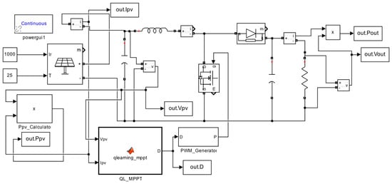
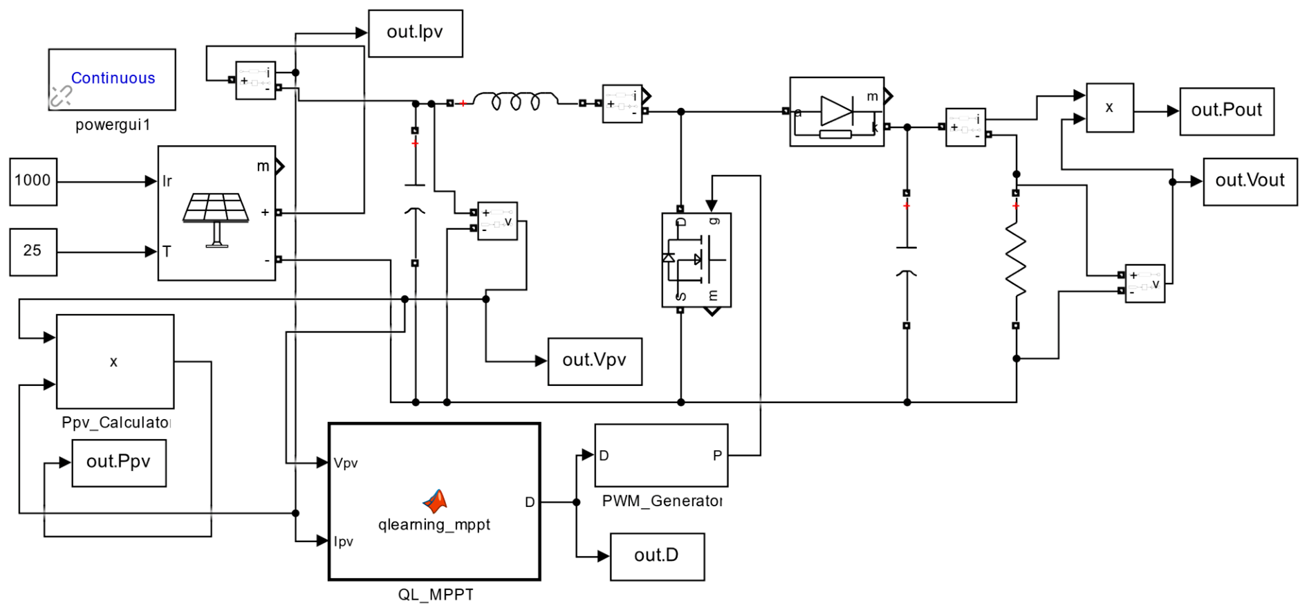
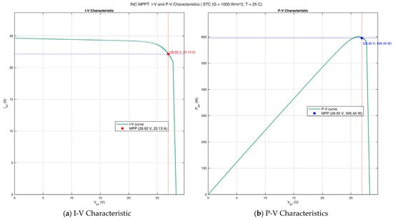
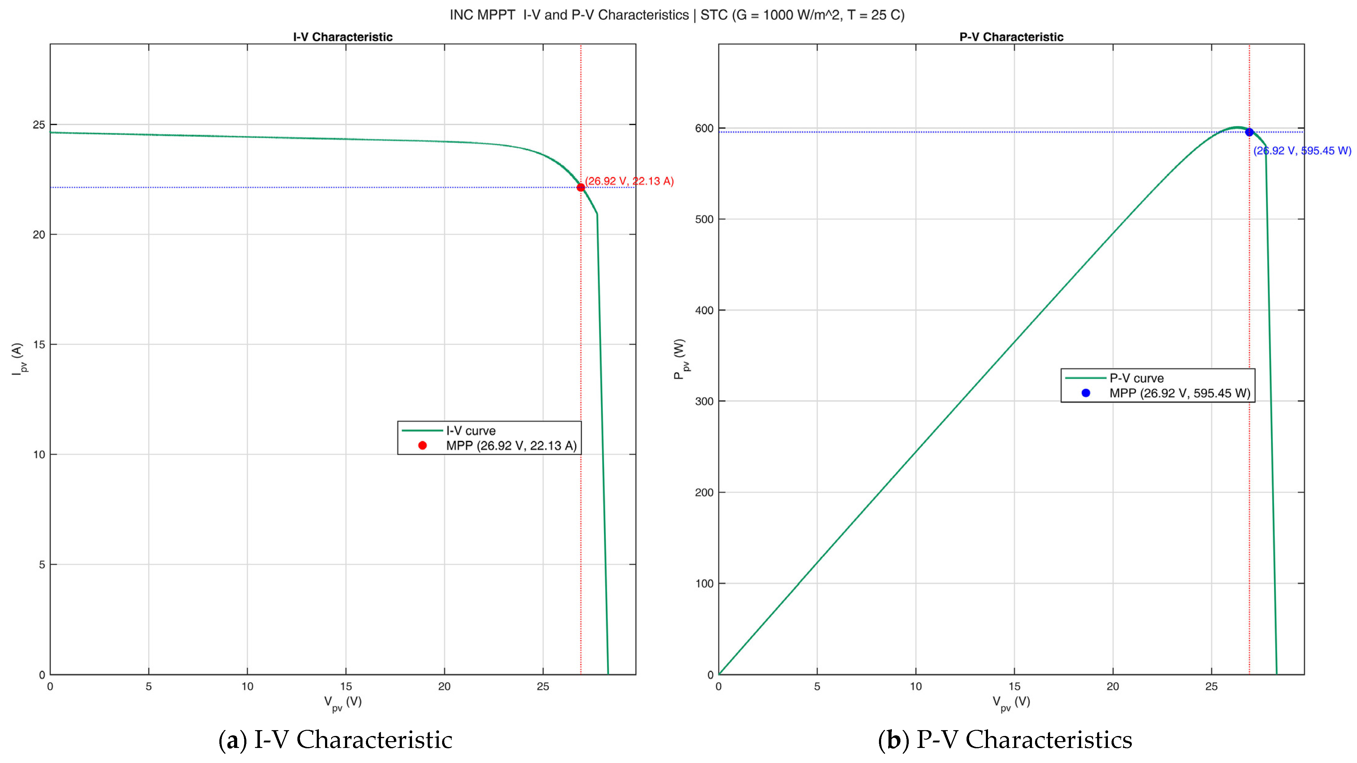
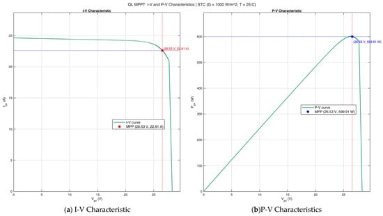
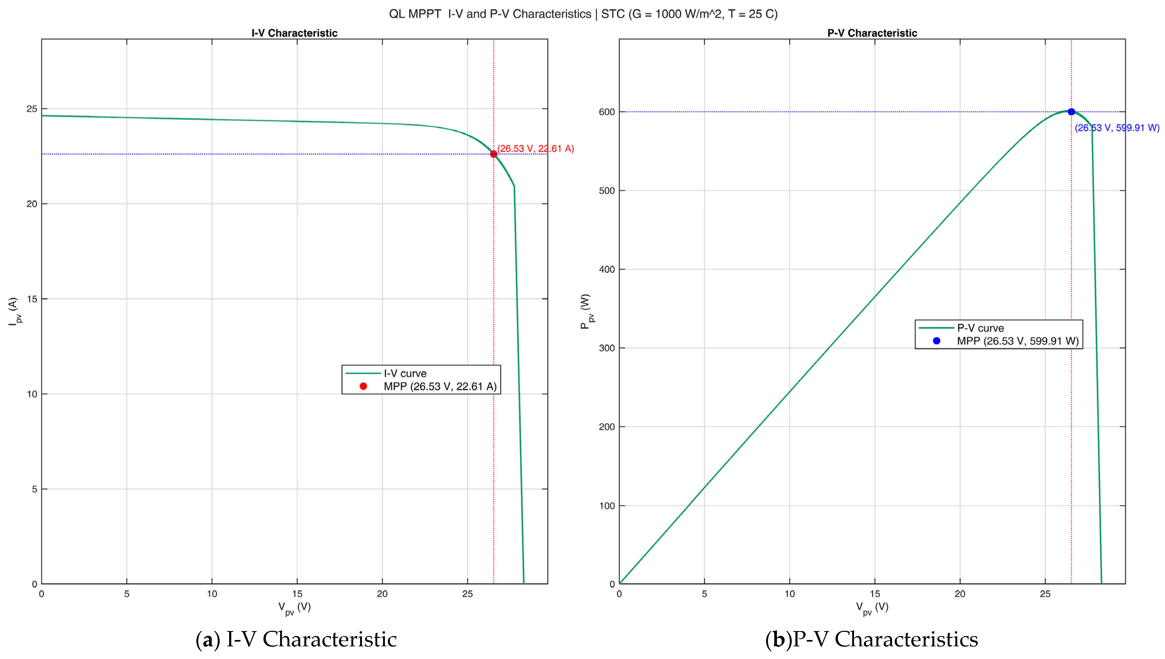
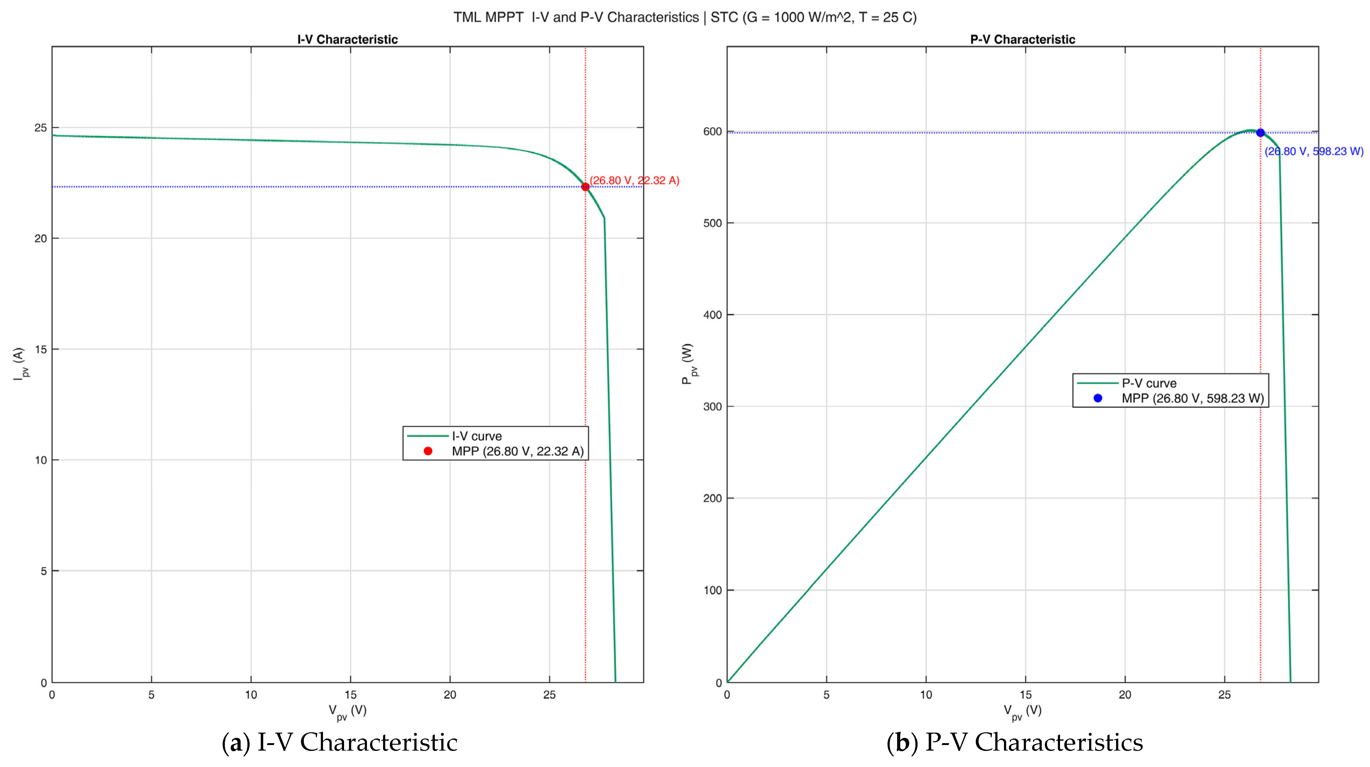
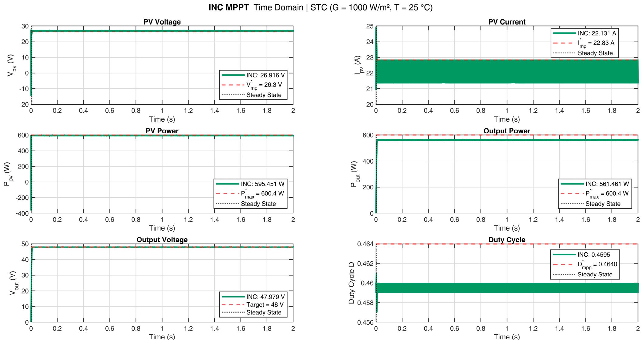
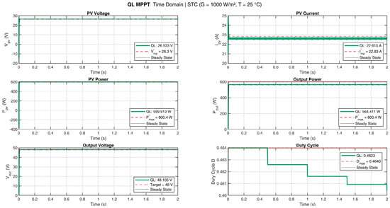
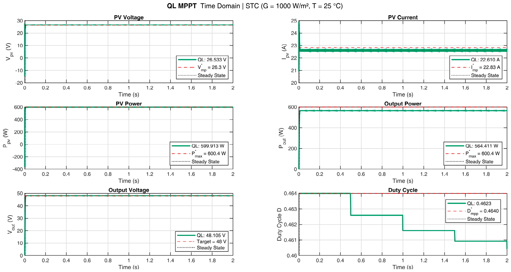
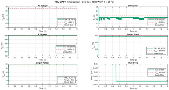
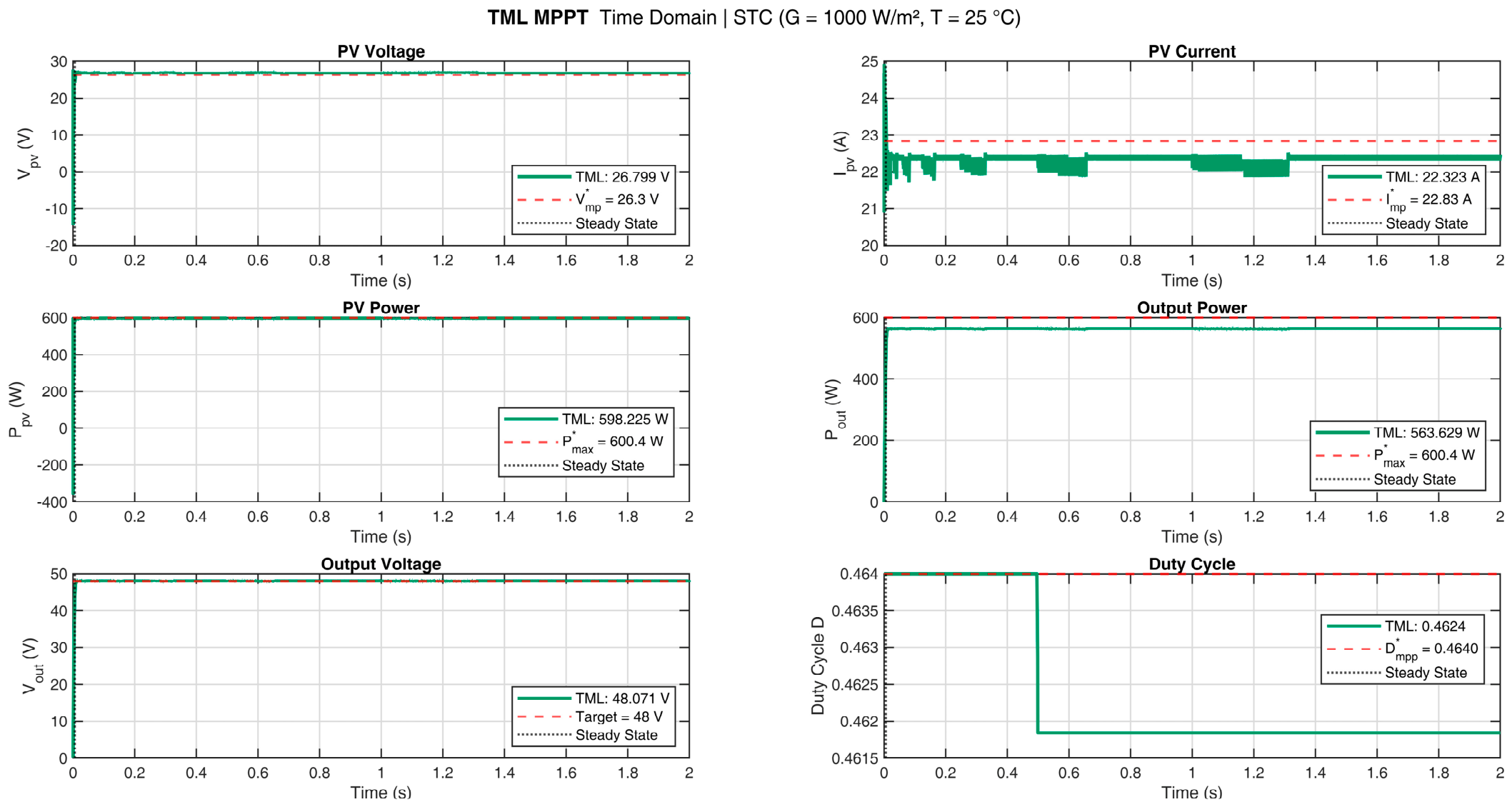
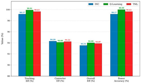
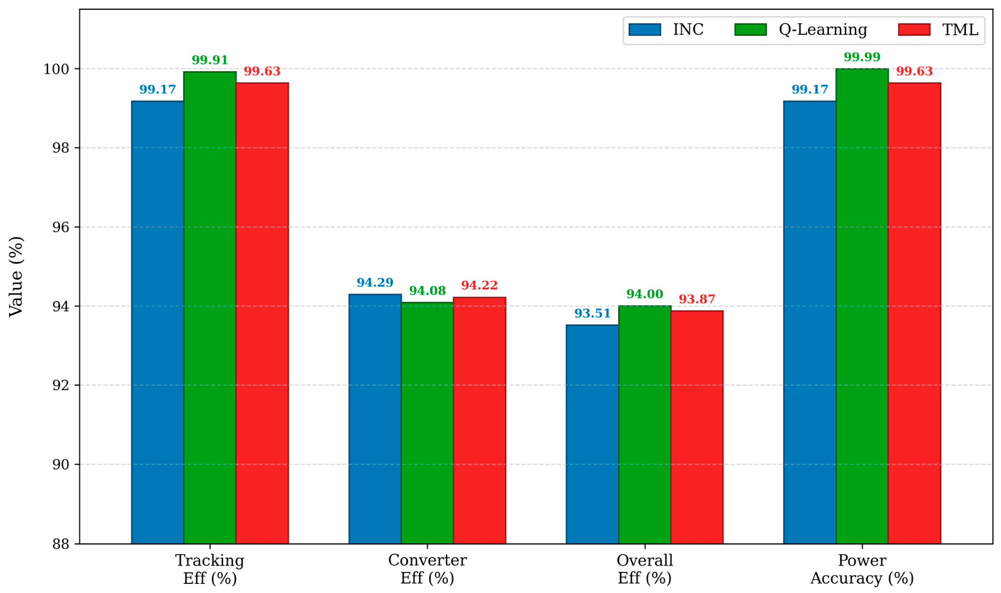
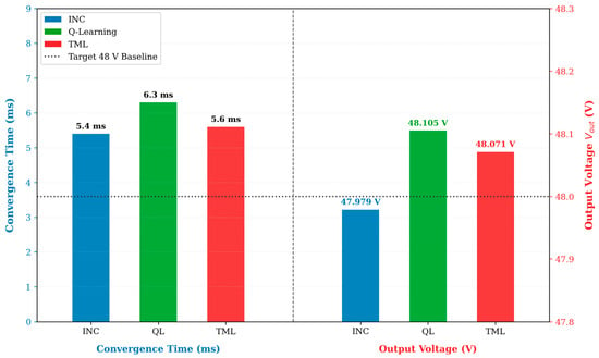
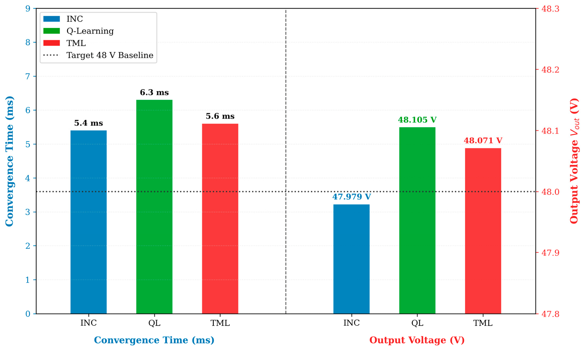
The steady-state performance metrics under standard test conditions (STC) are presented in Table 6. Figure 2 illustrates the complete simulation model of the proposed MPPT-controlled photovoltaic system under STC. Figure 3, Figure 4 and Figure 5 depict the current–voltage (I–V) and power–voltage (P–V) characteristic curves under STC for the evaluated tracking controllers. Furthermore, Figure 6, Figure 7 and Figure 8 show the time-domain responses of the MPPT controllers under STC, while Figure 9 presents a comparative analysis of the tracking efficiencies and accuracies. Figure 10 illustrates the convergence times (ms) and output voltages ($V_{out}$) under STC. All three algorithms exceed 99% tracking efficiency due to their robust steady-state capabilities under nominal conditions, with the tabular adaptive tracking approach achieving the highest tracking, converter, and overall efficiencies.

Table 6. STC steady-state performance: Scenario S1.

Metric	INC	Q-Learning	TML	Unit
$V_{pv}\left(\mathrm{V}\right)$	26.916	26.533	26.799	V
$I_{pv}\left(\mathrm{A}\right)$	22.131	22.610	22.323	A
$P_{pv}\left(\mathrm{W}\right)$	595.451	599.913	598.225	W
$V_{out}\left(\mathrm{V}\right)$	47.979	48.105	48.071	V
$P_{out}\left(\mathrm{W}\right)$	561.461	564.411	563.629	W
Tracking Efficiency (%)	99.171	99.914	99.633	%
Converter Efficiency (%)	94.292	94.084	94.217	%
Overall Efficiency (%)	93.510	94.001	93.871	%
Power Accuracy (%)	99.172	99.986	99.633	%
Duty Cycle D	0.4595	0.4623	0.4582	—
$\left|D-D_{mpp}\right|$ Error	0.0045	0.0017	0.0058	—
$V_{out}\left(V\right)$ Error from 48 V	0.021 V low	0.105 V high	0.071 V high	V
Convergence Time	5.4 ms	6.3 ms	5.6 ms	ms

Figure 2. MATLAB/Simulink model of the proposed MPPT-controlled system at STC.

Figure 3. INC MPPT characteristic curves at standard test condition (STC).

Figure 4. Q-Learning MPPT characteristic curves at standard test condition (STC).

Figure 5. TML MPPT characteristic curves at standard test condition (STC).

Figure 6. Time-domain response of the proposed INC MPPT controller under STC (G = 1000  $\mathrm{W}/{\mathrm{m}}^2$, T = 25 °C).

Figure 7. Time-domain response of the proposed Q-L MPPT controller under STC (G = 1000  $\mathrm{W}/{\mathrm{m}}^2$, T = 25 °C).

Figure 8. Time-domain response of the proposed TML MPPT controller under STC (G = 1000 $\mathrm{W}/{\mathrm{m}}^2$, T = 25 °C).

Figure 9. Comparative steady-state performance of the MPPT techniques in terms of tracking efficiency, converter efficiency, overall efficiency, and power accuracy under standard test conditions (G = 1000  $\mathrm{W}/{\mathrm{m}}^2$, T = 25 °C).

Figure 10. Performance comparison of the INC, Q-Learning, and TML MPPT algorithms in terms of convergence time (ms) and output voltage (V) under STC relative to the 48 V target.

4.2. Scenario S2: Irradiance Variation (T = 25 °C, G = 600–1200 W/m²)

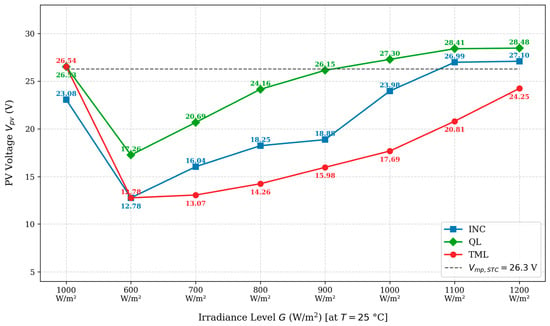
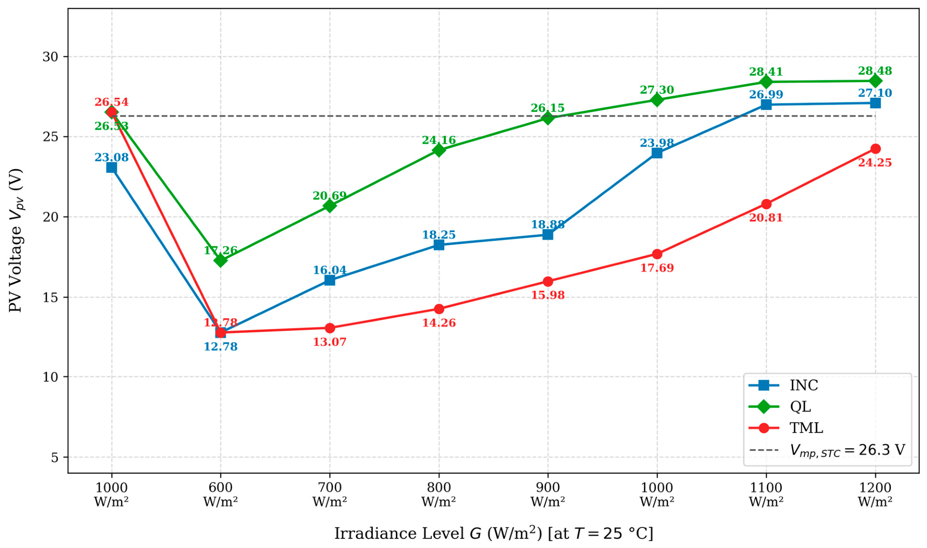
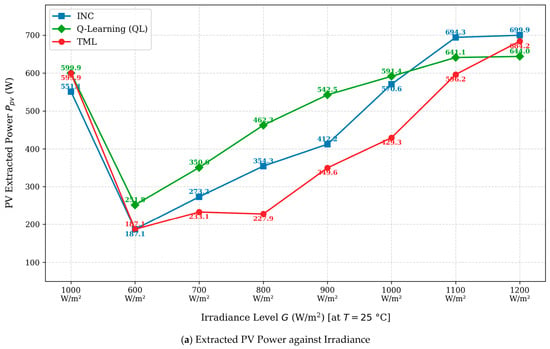
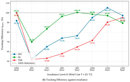
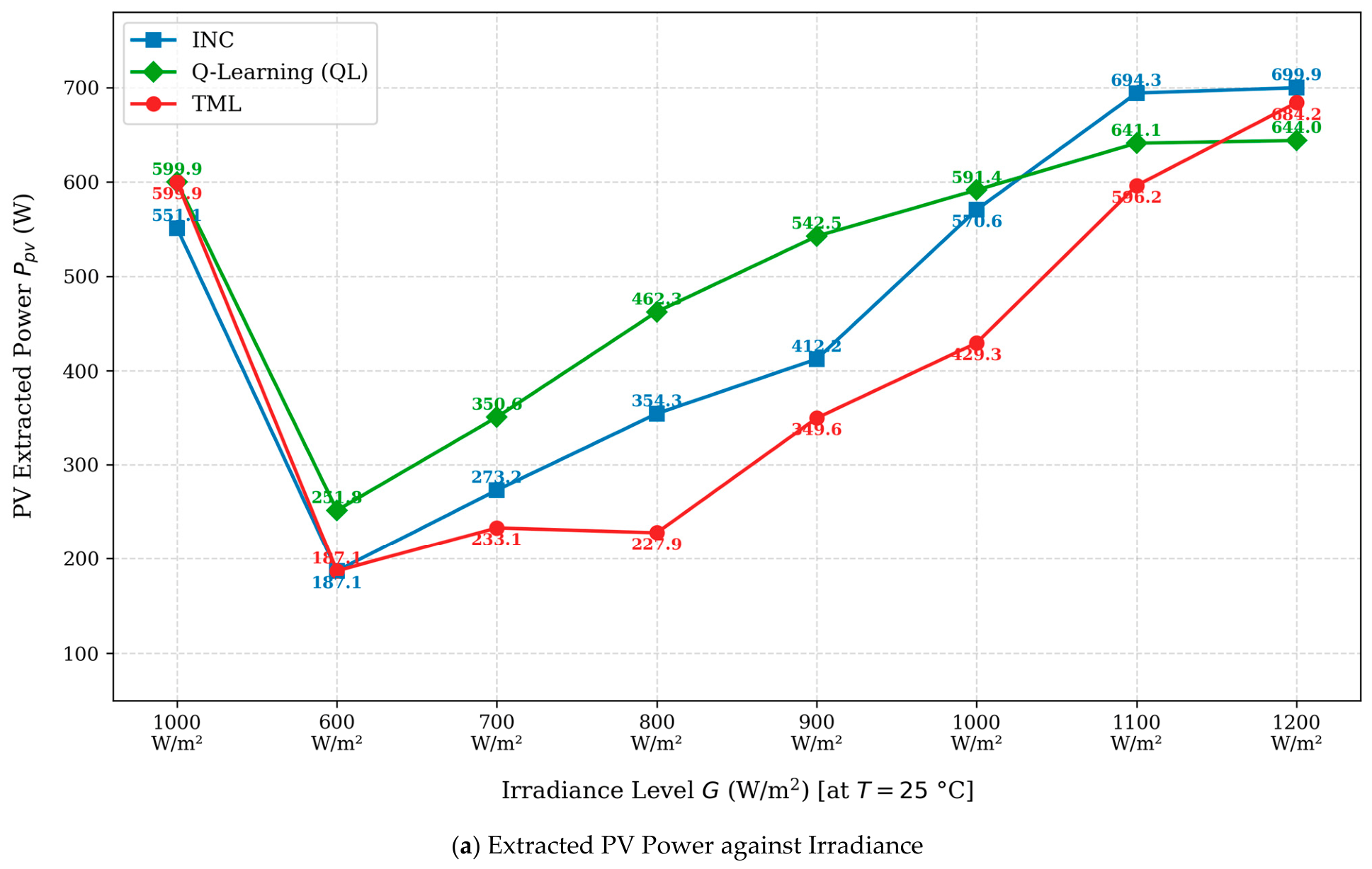
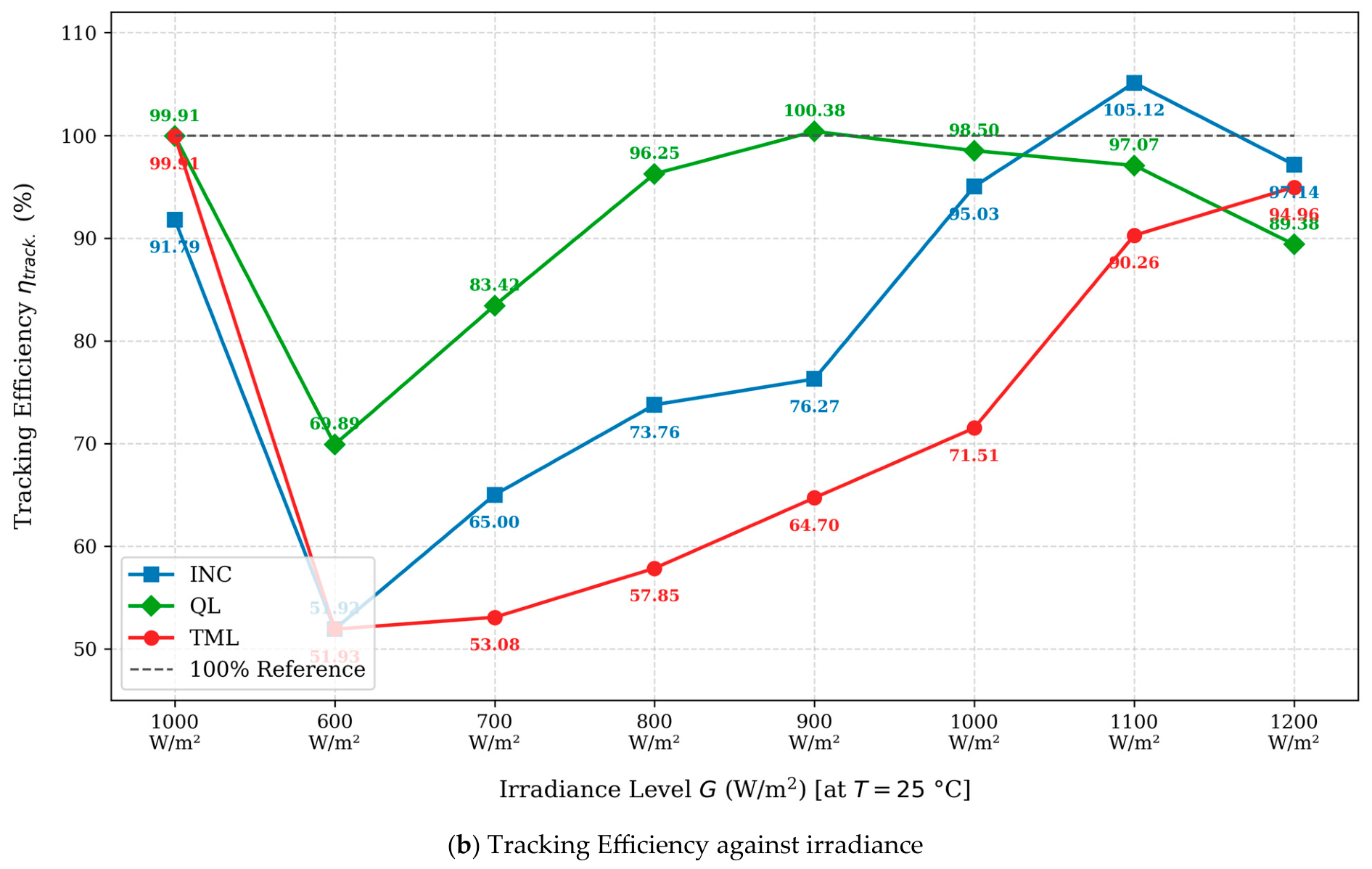
The second scenario (S2) examines the impact of irradiance fluctuations by stepping through eight distinct levels (600 to 1200 $\mathrm{W}/{\mathrm{m}}^2$) under a constant temperature of 25 °C. Table 7, Table 8, Table 9 and Table 10 list the per-phase performance metrics of the tracking algorithms, while Table 11 summarizes the average metrics across all eight phases. Figure 11 shows the effect of irradiance variation on PV voltage-tracking performance. Additionally, Figure 12 illustrates the performance comparison of the evaluated MPPT methods under dynamic irradiance conditions, depicting (a) the extracted PV power response and (b) the tracking efficiency performance.

Table 7. (S2): Per-phase (Ph) (G W/m², T $°\mathrm{C}$) $V_{pv}\left(\mathrm{V}\right)$ and $I_{pv}\left(\mathrm{A}\right)$ at T: 25 °C; G: 600–1200 $\mathrm{W}/{\mathrm{m}}^2$.

Ph	G (W/m2)	T (°C)	${\mathit{V}}_{\mathit{p}\mathit{v}}$ (V)			${\mathit{I}}_{\mathit{p}\mathit{v}}$ (A)
			INC	QL	TML	INC	QL	TML
1	1000	25	23.083	26.534	26.535	23.899	22.609	22.809
2	600	25	12.778	17.264	12.779	14.639	14.585	14.639
3	700	25	16.043	20.686	13.069	17.029	16.951	17.071
4	800	25	18.245	24.160	14.259	19.420	19.136	19.486
5	900	25	18.882	26.152	15.976	21.830	20.742	21.886
6	1000	25	23.984	27.298	17.686	23.803	21.666	24.276
7	1100	25	26.992	28.412	20.809	25.732	22.566	28.648
8	1200	25	27.101	28.475	24.249	25.837	22.616	22.108

Table 8. (S2): Per-phase (Ph) (G W/m², T $°\mathrm{C}$) $P_{pv}\left(\mathrm{W}\right)$ and $P_{out}\left(\mathrm{W}\right)$ at T: 25 °C; G: 600–1200 $\mathrm{W}/{\mathrm{m}}^2$.

Ph	G (W/M2)	T (°C)	${\mathit{P}}_{\mathit{p}\mathit{v}}$ (W)			${\mathit{P}}_{\mathit{o}\mathit{u}\mathit{t}}$ (W)
			INC	QL	TML	INC	QL	TML
1	1000	25	551.12	599.91	599.91	510.62	564.47	564.43
2	600	25	187.06	251.79	187.07	169.43	234.88	169.43
3	700	25	273.21	350.63	223.08	250.59	328.88	199.62
4	800	25	354.32	462.32	227.86	325.91	436.06	248.13
5	900	25	412.18	542.45	349.64	376.77	512.35	313.02
6	1000	25	570.57	591.44	429.34	530.47	559.01	385.13
7	1100	25	694.28	641.12	596.17	648.54	606.31	536.11
8	1200	25	699.93	643.98	684.18	653.93	609.07	627.37

Table 9. (S2): Per-phase (Ph) (G W/m², T $°\mathrm{C}$) $V_{out}\left(\mathrm{V}\right)$ and $D$ at T: 25 °C; G: 600–1200 $\mathrm{W}/{\mathrm{m}}^2$.

Ph	G (W/m2)	T (°C)	${\mathit{V}}_{\mathit{o}\mathit{u}\mathit{t}}$ (V)			Duty Cycle (D)
			INC	QL	TML	INC	QL	TML
1	1000	25	45.723	48.107	48.105	0.5207	0.4607	0.4608
2	600	25	26.357	31.033	26.356	0.5571	0.4651	0.5576
3	700	25	32.053	36.715	28600	0.5322	0.4600	0.5840
4	800	25	36.554	42.833	31.896	0.5280	0.4567	0.5990
5	900	25	39.303	45.833	35.824	0.5410	0.4589	0.5995
6	1000	25	46.625	47.874	39.737	0.5102	0.4590	0.5992
7	1100	25	51.565	49.858	46.882	0.4995	0.4571	0.5901
8	1200	25	51.779	49.972	50.702	0.4995	0.4552	0.5537

Table 10. (S2): Per-phase (Ph) (G W/m², T $°\mathrm{C}$) ${\eta }_{track.}(\%)$, ${\eta }_{conv.}(\%)$ and ${\eta }_{over.}(\%)$ at T: 25 °C; G: 600–1200 $\mathrm{W}/{\mathrm{m}}^2.$

Ph	G (W/m2)	T (°C)	Tracking Efficiency ${\mathit{\eta }}_{\mathit{t}\mathit{r}\mathit{a}\mathit{c}\mathit{k}.}$(%)			Converter Efficiency ${\mathit{\eta }}_{\mathit{c}\mathit{o}\mathit{n}\mathit{v}.}$(%)			Overall Efficiency ${\mathit{\eta }}_{\mathit{o}\mathit{v}\mathit{e}\mathit{r}.}$(%)
			INC	QL	TML	INC	QL	TML	INC	QL	TML
1	1000	25	91.788	99.914	99.914	92.651	94.091	94.085	85.043	94.010	94.004
2	600	25	51.923	69.893	51.926	90.578	93.284	90.572	47.031	65.199	47.030
3	700	25	65.003	83.423	53.075	91.722	93.798	89.483	59.622	78.250	47.493
4	800	25	73.764	96.248	57.846	91.983	94.319	89.303	67.850	90.780	51.658
5	900	25	76.274	100.383	64.703	91.410	94.450	89.524	69.722	94.812	57.924
6	1000	25	95.028	98.503	71.506	92.971	94.517	89.701	88.348	93.102	64.142
7	1100	25	105.118	97.071	90.264	93.412	94.570	89.926	98.193	91.799	81.170
8	1200	25	97.142	89.378	94.957	93.429	94.580	91.697	90.759	84.533	87.073

Table 11. Average performance across all phases S2 (T = 25 °C, G = 600–1200  $\mathrm{W}/{\mathrm{m}}^2$).

Metric	INC	Q-Learning	TML
Average Tracking Efficiency (%)	82.00	91.851	73.024
Average Converter Efficiency (%)	92.27	94.201	90.536
Average Overall Efficiency (%)	75.82	86.561	66.312
Average Duty Cycle D	0.5235	0.4591	0.5680
Average Convergence Time (s)	0.0369	0.0210	0.1958
$\mathrm{Average}{\mathrm{P}}_{\mathrm{p}\mathrm{v}}$ (W)	467.83	510.46	418.41
$\mathrm{Average}{\mathrm{P}}_{\mathrm{o}\mathrm{u}\mathrm{t}}$ (W)	433.28	481.38	380.40
Std Dev.-Tracking Efficiency (pp)	$\pm$18.2	$\pm 1$0.6	$\pm$19.4

Figure 11. (S2): Effect of irradiance variation on PV voltage-tracking performance.

Figure 12. (S2): Performance comparison of the evaluated MPPT methods under varying irradiance conditions: (a) extracted PV power response and (b) tracking efficiency performance.

4.3. Scenario S3: Temperature Variation (G = 1000 W/m², T = 0–75 °C)

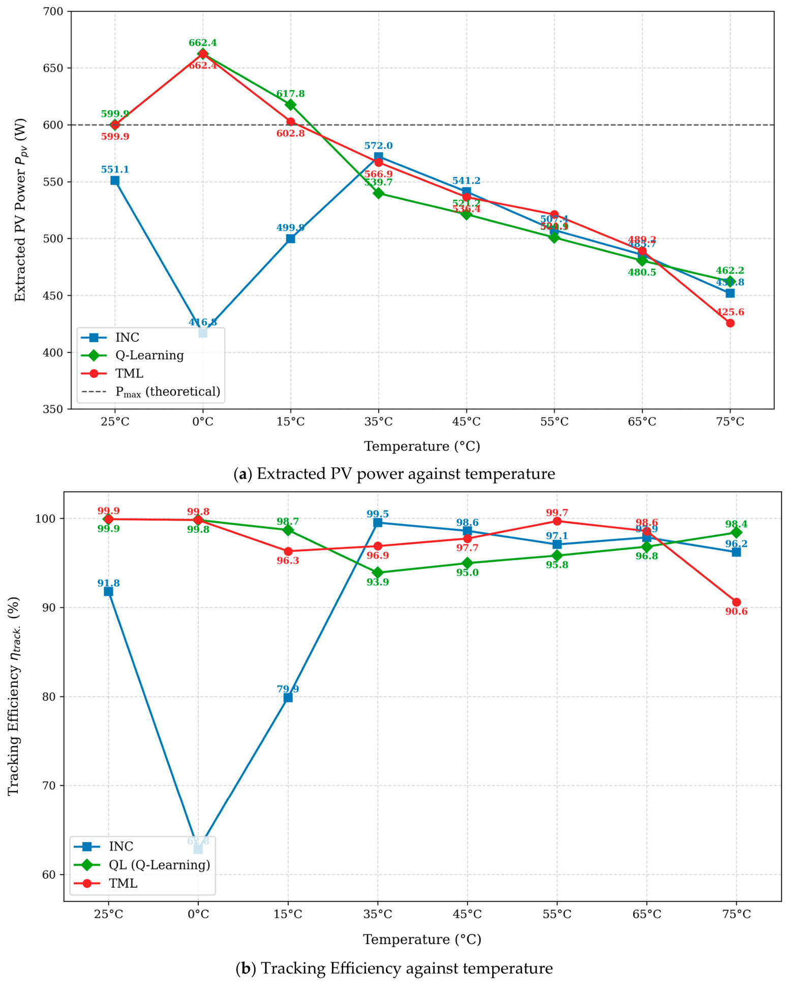
In Scenario S3, irradiance is fixed at 1000 W/m², while temperature is varied from 0 °C to 75 °C in eight increment steps. Table 12, Table 13, Table 14 and Table 15 present the per-phase performance of the algorithms in terms of voltage, current, power, efficiency, and duty cycle, while Table 16 summarizes the average performance metrics. Figure 13 shows the effect of temperature variation on MPPT performance, depicting (a) extracted PV power response and (b) tracking efficiency.

Table 12. (S3): Per-phase (Ph) (G W/m², T $°\mathrm{C}$) $V_{pv}\left(\mathrm{V}\right)$ and $I_{pv}\left(\mathrm{A}\right)$ (G = 1000 W/m², T = 0–75 °C).

Ph	G (W/m2)	T (°C)	${\mathit{V}}_{\mathit{p}\mathit{v}}$ (V)			${\mathit{I}}_{\mathit{p}\mathit{v}}$ (A)
			INC	QL	TML	INC	QL	TML
1	1000	25	23.083	26.534	26.535	23.899	22.609	22.609
2	1000	0	17.427	28.877	28.878	23.915	22.940	22.939
3	1000	15	20.777	28.361	28.982	24.062	21.789	20.806
4	1000	35	25.449	26.997	26.496	22.486	19.991	21.018
5	1000	45	24.758	25.640	25.099	21.866	20.330	21.373
6	1000	55	24.009	24.298	23.007	21.141	20.614	22.651
7	1000	65	22.609	22.915	20.556	21.490	20.970	23.800
8	1000	75	21.814	21.241	17.241	20.722	21.769	24.689

Table 13. (S3): Per-phase (ph) (G W/m², T $°\mathrm{C}$) $P_{pv}\left(\mathrm{W}\right)$ and $P_{out}\left(\mathrm{W}\right)$ (G = 1000 W/m², T = 0–75 °C).

Ph	G (W/m2)	T (°C)	${\mathit{P}}_{\mathit{p}\mathit{v}}$ (W)			${\mathit{P}}_{\mathit{o}\mathit{u}\mathit{t}}$ (W)
			INC	QL	TML	INC	QL	TML
1	1000	25	551.12	599.92	599.91	510.62	564.47	564.43
2	1000	0	416.76	662.42	662.42	373.77	626.65	626.61
3	1000	15	499.93	617.76	602.84	457.78	585.30	573.26
4	1000	35	572.05	539.70	566.88	536.64	511.82	526.06
5	1000	45	541.16	521.25	536.41	507.41	492.16	504.18
6	1000	55	507.40	500.85	521.11	475.58	470.54	484.37
7	1000	65	485.66	480.52	489.23	452.42	448.93	447.87
8	1000	75	451.84	462.23	425.55	420.64	427.69	379.75

Table 14. (S3): Per-phase (Ph) (G W/m², T $°\mathrm{C}$) $V_{out}\left(\mathrm{V}\right)$ and $D$ (G = 1000 W/m², T = 0–75 °C).

Ph	G (W/m2)	T ($\mathbf{°}\mathbf{C}$)	${\mathit{V}}_{\mathit{o}\mathit{u}\mathit{t}}$ (V)			Duty Cycle (D)
			INC	QL	TML	INC	QL	TML
1	1000	25	45.723	48.107	4105	0.5207	0.4627	0.4602
2	1000	0	39.146	50.688	50.686	0.5880	0.4522	0.4406
3	1000	15	43.323	48.987	48.479	0.5577	0.4381	0.4229
4	1000	35	46.906	45.809	46.441	0.4795	0.4354	0.4423
5	1000	45	45.611	44.920	45.446	0.4795	0.4453	0.4783
6	1000	55	44.157	43.923	44.563	0.4795	0.4723	0.5158
7	1000	65	43.069	42.902	42.851	0.4995	0.4914	0.5453
8	1000	75	41.528	41.875	39.450	0.4995	0.5212	0.5975

NB: One MPPT cycle = minimum measurable t_conv (values below 0.5 ms) indicate the algorithm entered the ±3% power convergence band within the first control cycle.

Table 15. (S3): Per-phase (Ph) (G W/m², T $°\mathrm{C}$) ${\eta }_{track.}(\%)$, ${\eta }_{conv.}(\%)$ and ${\eta }_{over.}(\%)$ at T: 25 °C; G: 600–1000 W/m².

Ph	G (W/m2)	T (°C)	Tracking Efficiency ${\mathit{\eta }}_{\mathit{t}\mathit{r}\mathit{a}\mathit{c}\mathit{k}}.$(%)			Converter Efficiency ${\mathit{\eta }}_{\mathit{c}\mathit{o}\mathit{n}\mathit{v}.}$(%)			Overall Efficiency ${\mathit{\eta }}_{\mathit{o}\mathit{v}\mathit{e}\mathit{r}.}$(%)
			INC	QL	TML	INC	QL	TML	INC	QL	TML
1	1000	25	91.788	99.914	99.914	92.651	94.091	94.085	85.043	94.010	92.004
2	1000	0	62.801	99.818	99.819	89.683	94.600	94.594	56.322	94.428	94.423
3	1000	15	79.876	98.702	96.319	91.569	94.746	95.093	73.142	93.516	91.592
4	1000	35	99.532	93.903	96.893	93.809	94.835	94.464	93.370	89.053	91.530
5	1000	45	98.604	94.978	97.740	93.764	94.418	93.992	92.456	89.676	91.868
6	1000	55	97.081	95.828	99.703	93.729	93.948	92.951	90.993	90.029	92.675
7	1000	65	97.864	96.827	98.582	93.156	93.426	91.546	91.166	90.462	90.247
8	1000	75	96.211	98.422	90.613	93.095	92.529	89.236	89.568	91.069	80.860

Table 16. (S3): Average performance across all phases—S3 (G = 1000 W/m², T = 0–75 °C).

Metric	INC	Q-Learning	TML
Average Tracking Efficiency (%)	90.470	97.299	97.448
Average Converter Efficiency (%)	92.682	94.074	93.245
Average Overall Efficiency (%)	84.007	91.531	90.900
Average Duty Cycle D	0.5130	0.4648	0.4879
Average Convergence Time (s)	0.0686	0.0997	0.1248
Average ${\mathrm{P}}_{\mathrm{p}\mathrm{v}}$ (W)	503.24	548.08	549.30
Average  ${\mathrm{P}}_{\mathrm{o}\mathrm{u}\mathrm{t}}$  (W)	466.86	515.95	513.32
Std Dev.—Tracking Efficiency (pp)	$\pm$12.9	$\pm$2.3	$\pm$3.1

Figure 13. (S3): Effect of temperature variation on MPPT performance: (a) extracted PV power response and (b) tracking efficiency.

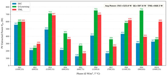
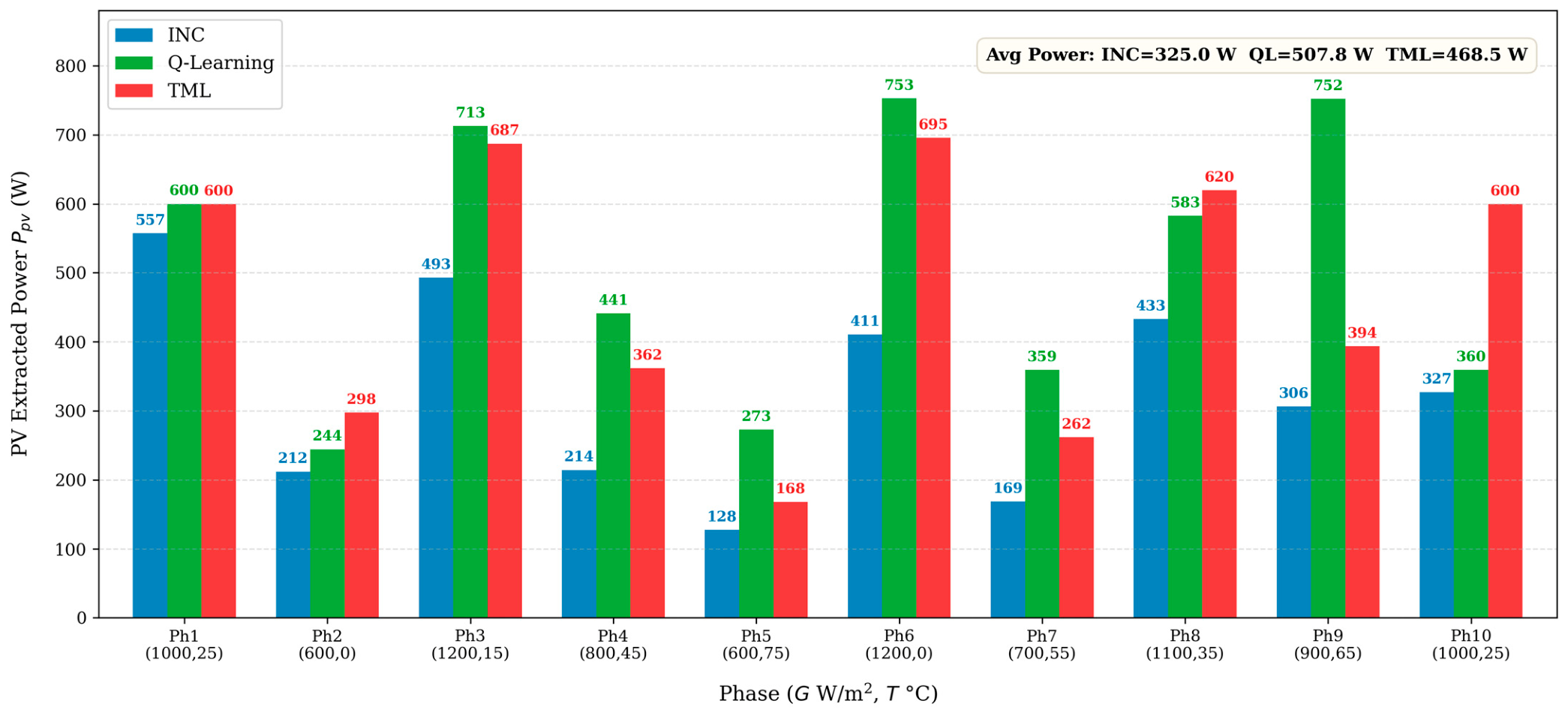
4.4. Scenario S4: Wide-Range Simultaneous G-T Variation (G = 600–1200 W/m², T = 0–75 °C)

Scenario S4 constitutes the most demanding evaluation with simultaneous irradiance and temperature variation across their full ranges over ten phases. Under these conditions, both the available power and the optimal operating voltage vary concurrently.

Table 17, Table 18, Table 19, Table 20 and Table 21 present per-phase and summarized performance results, while Table 22 presents the average performance statistics. Figure 14 compares the extracted PV power performance of the INC, Q-Learning, and TML MPPT methods under varying irradiance and temperature operating conditions.

Table 17. Per- phase (Ph) (G W/m², T $°\mathrm{C}$) $V_{pv}$ (V) and $I_{pv}$ (A)—S4 (wide-range G = 600–1200 W/m², T = 0–75 °C).

Ph	G (W/m2)	T (°C)	${\mathit{V}}_{\mathit{p}\mathit{v}}$ (V)			${\mathit{I}}_{\mathit{p}\mathit{v}}$ (A)
			INC	QL	TML	INC	QL	TML
1	1000	25	23.386	26.534	26.535	26.353	22.620	22.609
2	600	0	14.713	16.998	20.793	14.395	14.367	14.322
3	1200	15	17.033	28.891	29.407	28.959	24.671	23.366
4	800	45	10.821	23.597	18.438	19.777	18.699	19.629
5	600	75	8.437	18.594	11.120	15.133	14.661	15.098
6	1200	0	14.278	30.751	31.651	28.760	24.473	21.971
7	700	55	9.675	21.321	15.077	17.428	16.861	17.347
8	1100	35	16.111	27.089	25.993	26.894	21.517	23.836
9	900	65	13.642	23.241	17.698	22.449	18.411	22.246
10	1000	25	13.418	26.526	26.535	24.363	22.617	22.609

Table 18. Per-phase (Ph) (G W/m²,T $°\mathrm{C}$) $P_{pv}$ (W) and $P_{out}$ (W)—S4 (wide-range G = 600–1200 W/m², T = 0–75 °C).

Ph	G (W/m2)	T (°C)	${\mathit{P}}_{\mathit{p}\mathit{v}}$ (W)			${\mathit{P}}_{\mathit{o}\mathit{u}\mathit{t}}$ (W)
			INC	QL	TML	INC	QL	TML
1	1000	25	557.38	599.96	599.91	516.28	563.83	564.43
2	600	0	211.79	244.22	297.79	194.95	227.45	281.79
3	1200	15	493.25	712.75	687.12	430.07	670.71	650.15
4	800	45	214.00	441.24	361.92	182.25	415.50	332.96
5	600	75	127.68	272.61	167.90	108.15	255.41	148.96
6	1200	0	410.63	752.55	695.40	346.09	711.75	663.19
7	700	55	168.62	359.49	261.53	143.44	337.84	237.90
8	1100	35	433.28	582.85	619.55	378.10	550.18	580.00
9	900	65	306.25	752.25	393.72	266.80	402.82	356.53
10	1000	25	326.90	359.64	599.91	280.34	563.82	564.43

Table 19. Per-phase (Ph) (G W/m², T $°\mathrm{C}$) $V_{out}$ (V) and $D$—S4 (wide-range G = 600–1200 W/m², T = 0–75 °C).

Ph	G (W/m2)	T (°C)	${\mathit{V}}_{\mathit{o}\mathit{u}\mathit{t}}$ (V)			Duty Cycle (D)
			INC	QL	TML	INC	QL	TML
1	1000	25	45.978	48.080	48.105	0.5160	0.4670	0.4658
2	600	0	28.272	30.538	33.990	0.5180	0.4611	0.4154
3	1200	15	41.979	52.439	51.629	0.6339	0.4610	0.4478
4	800	45	27.331	41.274	36.947	0.6564	0.4564	0.5312
5	600	75	21.057	32.360	24.713	0.6530	0.4508	0.5870
6	1200	0	37.669	54.020	52.145	0.6610	0.4508	0.4175
7	700	55	24.251	37.217	31.231	0.6526	0.4441	0.5591
8	1100	35	39.367	47.494	48.765	0.6341	0.4496	0.4856
9	900	65	33.074	40.639	38.233	0.6290	0.4561	0.5639
10	1000	25	33.902	48.080	48.105	0.6410	0.4628	0.4659

Table 20. Per-phase (Ph) (G W/m², T $°\mathrm{C}$) ${\eta }_{track.}$(%), ${\eta }_{conv.}$(%), and ${\eta }_{over.}$(%)—S4 (wide-range G = 600–1200 W/m², T = 0–75 °C).

Ph	G (W/m2)	T (°C)	Tracking Efficiency ${\mathit{\eta }}_{\mathit{t}\mathit{r}\mathit{a}\mathit{c}\mathit{k}.}$(%)			Converter Efficiency ${\mathit{\eta }}_{\mathit{c}\mathit{o}\mathit{n}\mathit{v}.}$(%)			Overall Efficiency ${\mathit{\eta }}_{\mathit{o}\mathit{v}\mathit{e}\mathit{r}.}$(%)
			INC	QL	TML	INC	QL	TML	INC	QL	TML
1	1000	25	92.830	100.02	100.02	92.626	93.978	94.085	85.985	93.997	94.097
2	600	0	68.700	66.036	80.524	92.050	94.101	94.626	54.115	61.503	76.196
3	1200	15	68.459	97.723	94.210	87.191	93.243	94.620	59.690	91.959	89.141
4	800	45	44.551	95.337	78.199	85.165	94.166	91.996	37.942	89.775	71.940
5	600	75	35.441	85.227	52.491	84.704	93.691	88.723	30.020	79.851	46.572
6	1200	0	56.991	101.745	94.018	94.577	94.394	95.368	48.033	96.228	89.663
7	700	55	40.120	90.867	66.106	85.067	93.977	90.965	34.128	85.394	60.133
8	1100	35	65.602	89.796	95.450	87.263	94.681	93.617	57.246	84.762	89.357
9	900	65	56.673	86.439	79.534	87.119	94.140	90.555	49.373	81.373	72.022
10	1000	25	54.445	100.016	77.812	100.013	93.981	94.085	56.353	93.996	94.097

Table 21. Average performance—S4 (G = 600–1200 W/m², T = 0–75 °C).

Metric	INC	Q-Learning	TML
Average Tracking Efficiency (%)	57.39	91.321	84.056
Average Converter Efficiency (%)	87.12	94.014	92.864
Average Overall Efficiency (%)	50.32	85.884	78.322
Average Duty Cycle D	0.6195	0.4560	0.4939
Average Convergence Time (s)	0.0331	0.00124	0.0837
Average  ${\mathrm{P}}_{\mathrm{p}\mathrm{v}}$  (W)	324.98	499.35	468.48
Average  ${\mathrm{P}}_{\mathrm{o}\mathrm{u}\mathrm{t}}$  (W)	284.65	469.93	438.03
Std Dev.—Tracking Efficiency (pp)	$\pm 16.7$	$\pm 10.6$	$\pm 14.8$

Table 22. Average efficiency comparison across all four scenarios (%).

Scenario	INC Track	QL Track	TML Track	INC Conv	QL Conv	TML Conv	INC Total	QL Total	TML Total
S1—STC	99.171	99.914	99.633	94.292	94.084	94.217	93.510	94.001	93.871
S2—Irradiance	82.005	91.851	73.024	92.270	94.201	90.536	75.821	86.561	66.312
S3—Temperature	90.470	97.299	97.448	92.682	94.074	93.245	84.007	91.531	90.900
S4—Wide-Range G+T	57.39	91.32	84.06	87.12	94.014	92.864	50.32	85.884	78.322
Std Dev Tracking Eff. (pp) [S2/S3/S4]	$\pm$18.2/$\pm$10.6/ $\pm$19.4	$\pm 1$2/$\pm$2.1/$\pm$2.9	$\pm$16.7/$\pm 10.6/\pm$14.8	$\pm 0.95/\pm$1.33/$\pm 4.80$	$\pm 1.99/\pm 0.73/\pm 0.37$	$\pm 0.43/\pm 1.84/\pm 2.07$	$\pm$16.43/$\pm$12.12/$\pm$15.11	$\pm$9.62/$\pm$1.99/$\pm 9.71$	$\pm 17.44/\pm$3.86/$\pm 15.13$

Figure 14. (S4): Extracted PV power characteristics of the evaluated MPPT methods across different irradiance and temperature phases.

4.5. Cross-Scenario Comparative Analysis

4.5.1. Efficiency Summary Across All Scenarios

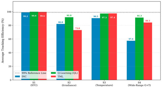
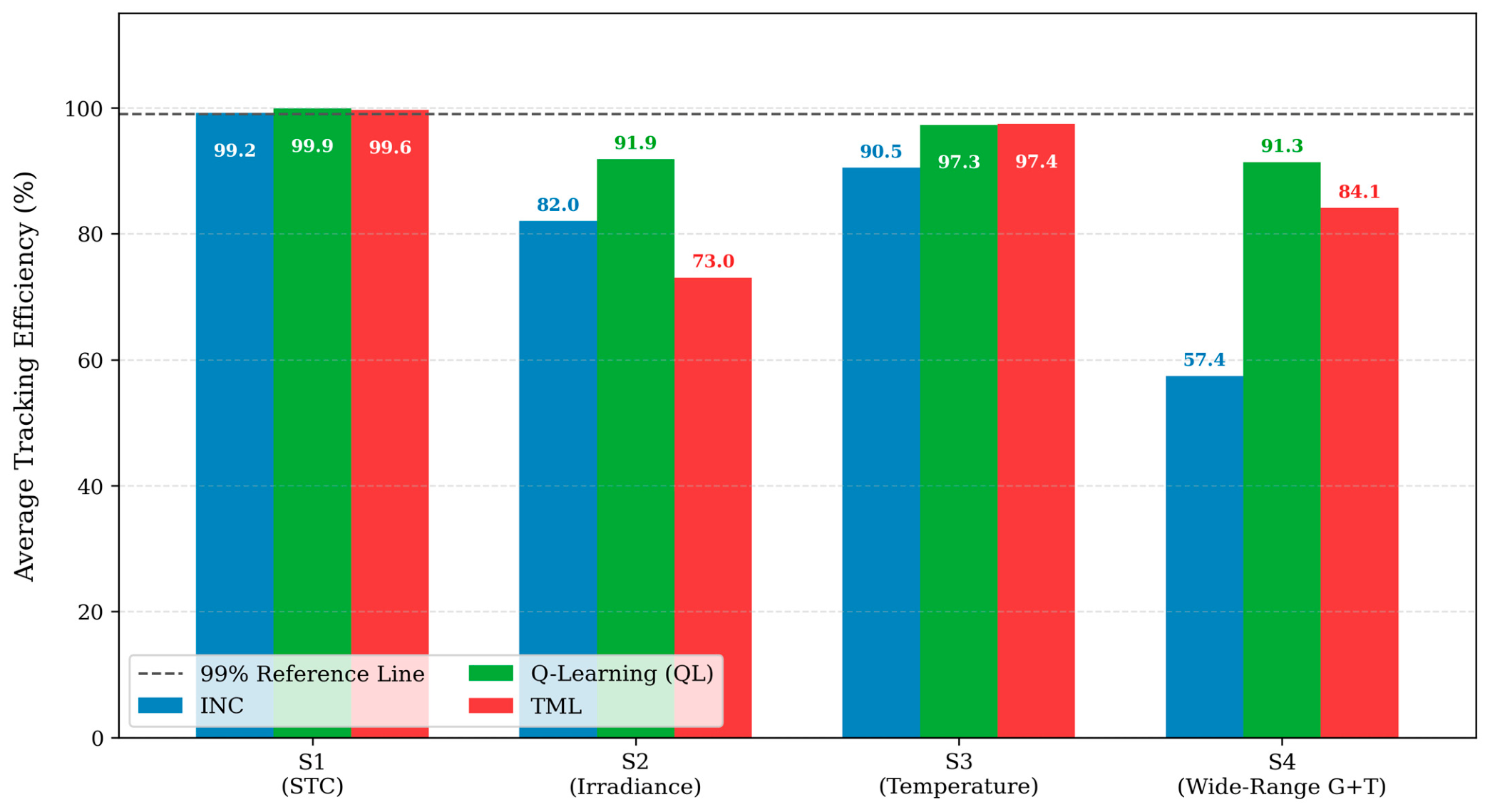
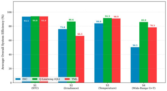
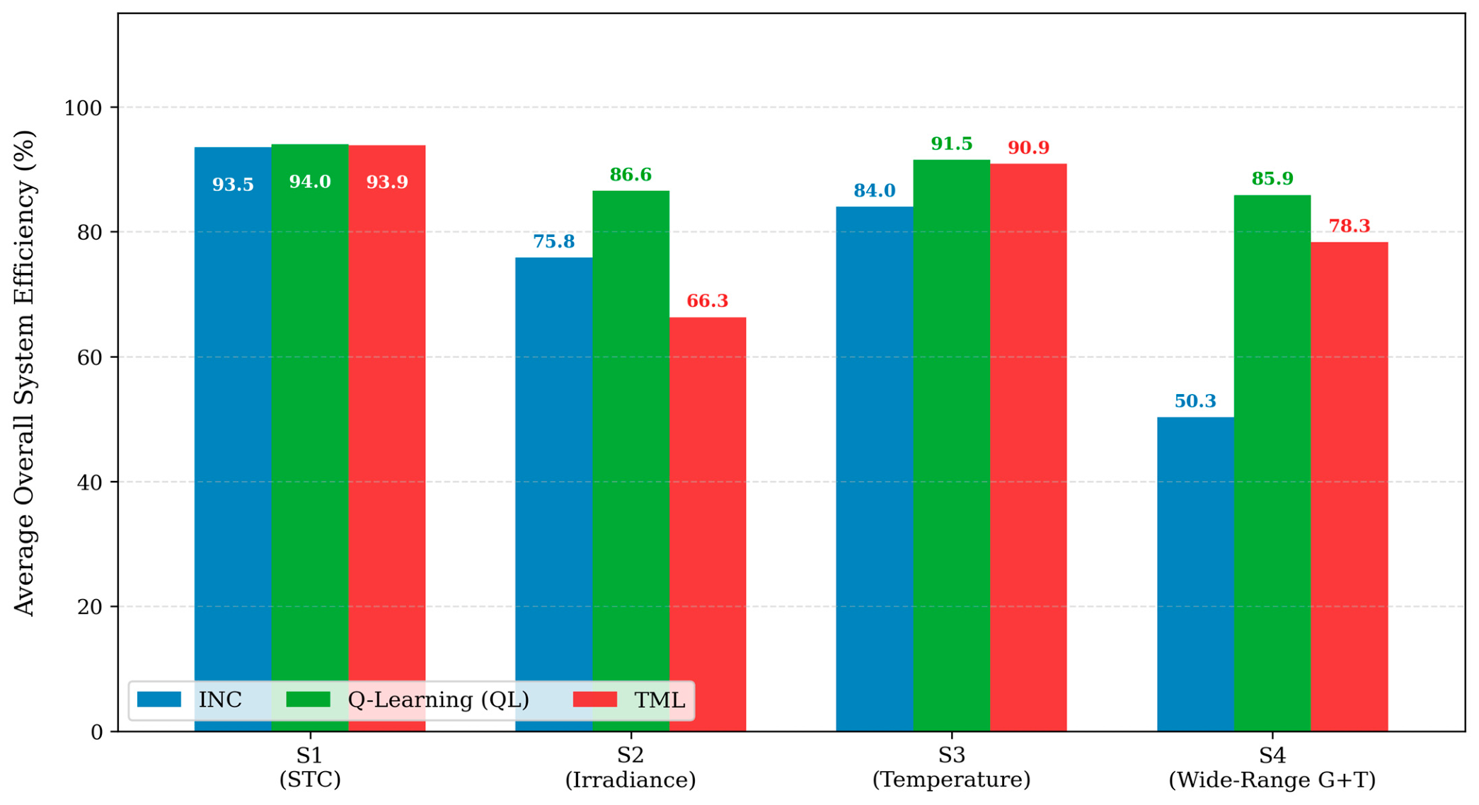
Table 22 summarizes the average tracking efficiency, converter efficiency, and overall system efficiency of the three evaluated algorithms across all four operating scenarios, thereby enabling assessment of performance consistency and degradation under increasing environmental complexity. Figure 15 compares the average tracking efficiency of the evaluated MPPT methods across the different operating scenarios, including STC, irradiance variation, temperature variation, and combined irradiance and temperature variations. Similarly, Figure 16 compares the average overall system efficiency of the evaluated MPPT methods under these respective operating scenarios.

Figure 15. Average tracking efficiency comparison of the evaluated MPPT methods under different operating scenarios.

Figure 16. Comparative analysis of overall system efficiency under varying environmental conditions.

4.5.2. Duty-Cycle Behavior and Voltage Regulation

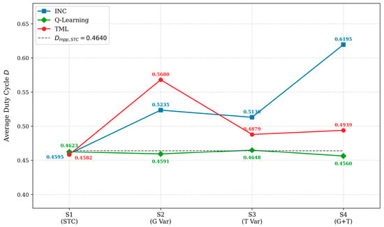
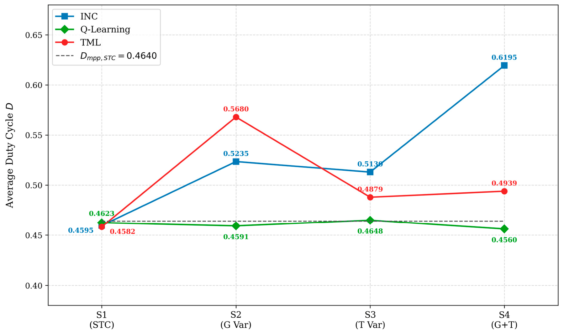
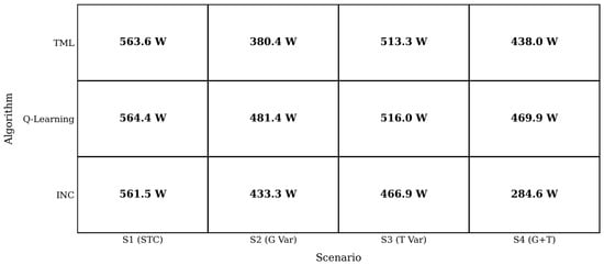
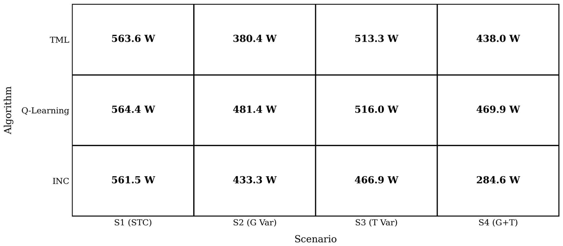
A particularly informative comparison is the average duty cycle across scenarios. Under standard test conditions (STC), all three algorithms correctly target a duty-cycle (D) near 0.4640. However, as operating conditions deviate from STC, the duty-cycle distributions of the evaluated algorithms diverge sharply. Figure 17 compares the average duty-cycle response of the evaluated MPPT methods across different operating scenarios, while Figure 18 compares the corresponding output power performance under these conditions. Under STC, the INC, Q-Learning, and TML methods achieved output voltages of 47.979 V, 48.105 V, and 48.071 V, respectively, all within 0.2 V of the nominal 48 V target. In Scenario S4, the average output voltage of the INC is 33.288 V, whereas Q-Learning and TML as an average output voltage of 43.21 V and 41.39 V respectively, demonstrating superior of load regulation performance under dynamic conditions.

Figure 17. Average duty-cycle response comparison of the evaluated MPPT methods under different operating scenarios.

Figure 18. Output power performance comparison across different operating scenarios.

5. Discussion and Results Analyses for Each Scenario

The simulation results across four operating scenarios are presented below. All values are obtained from MATLAB/Simulink closed-loop simulation of the KC200GT 1S×3P PV array with a DC–DC boost converter. In Scenario 1, under STC, all three algorithms achieve tracking efficiencies above 99% (INC: 99.171%, QL: 99.914%, TML: 99.633%), with an inter-algorithm spread of 0.743 pp, confirming that the single static operating point does not discriminate between MPPT strategies. QL attains the highest overall efficiency (94.001%) and the lowest duty-cycle deviation from the theoretical optimum D_mpp = 0.4640 ($\left|∆D\right|$ = 0.0017). INC achieves the shortest convergence time (5.4 ms), followed by TML (5.6 ms) and QL (6.3 ms); all three are well within any practical MPPT interrupt period. Output voltage $V_{out}$ is within 0.22% of the 48 V target for all algorithms, meeting standard regulation requirements. In Scenario 2, irradiance variation at constant temperature, QL achieves the highest average tracking efficiency (91.851%) and average P_pv (510.46 W), outperforming INC by 9.85 pp and TML by 18.83 pp because the Q-table lookup selects the duty-cycle action based on the observed power-gradient state, regardless of irradiance-step magnitude. In Scenario 3, temperature variation and constant irradiance, TML and QL achieve near-identical average tracking efficiencies (97.45% and 97.30%) and average P_pv (549.30 W and 548.08 W), outperforming INC (90.47%, 503.24 W). At fixed irradiance, both the sign-history state representation and the complement input feature (1–V_n) provide adequate thermal sensitivity to follow V_mp(T) shifts. QL exhibits the lowest inter-phase tracking standard deviation ($\pm$2.1 pp vs. TML $\pm$2.9 pp and INC $\pm$12.0 pp), confirming more consistent phase-to-phase performance. INC converges fastest (68.6 ms); INC converges fastest (68.6 ms) due to the direct gradient search. In Scenario 4, simultaneous irradiance and temperature variation, QL achieves the highest average tracking efficiency (91.321%) and average P_out (469.93 W) due to the 3D state space (V_bin, $∆$P_bin, T_bin) and the 1800-entry pre-seeded Q-table, which maps the temperature bin index to the correct duty-cycle direction within 1–2 update cycles. The TML and INC achieve average tracking efficiency and power of 84.056%, 438.03 W, and 57.390%, 284.65 W. The Scenario 4 results are the most operationally significant, as simultaneous irradiance and temperature variation is representative of realistic field conditions, including morning ramp-up, partial cloud cover, and seasonal temperature cycling. Under these conditions, QL extracts 39.4% more power than INC and 7.3% more than TML per simulated phase cycle. These simulation-derived rankings require hardware validation on a physical PV array to account for real converter dynamics, measurement noise, and component tolerances, as discussed in Section 5.1.

5.1. Algorithm Selection Guide

Based on the results, Table 23 presents the summary of MPPT algorithm selection for a real-life scenario under variable climate conditions for PV installation.

Table 23. Summarized MPPT algorithms results based on performance for practical deployment in real-life scenarios.

Deployment Scenario	Dominant Signal	Recommended Algorithm	Rationale
Narrow operating range/STC	Stable	Any (INC preferred)	All algorithms exceed 99% tracking efficiency. INC preferred: no offline training or dataset required; fastest convergence.
Pure irradiance variation (T = const)	$I_{pv}$ variation	QL	Irradiance drives a proportional change in Imp at fixed Vmp; the sign-history state captures the power-gradient direction within 1–2 sampling intervals, independent of the irradiance-step magnitude.
Pure temperature variation (G = const)	$V_{pv}$ variation	TML (QL also acceptable)	9.2 V $V_{mp}$ range gives rich $V_n$ signal for attention.
Combined G–T variation (real outdoor)	Both	TML strongly preferred	Continuous $D^{*}\left(G,T\right)$ mapping; 16.7 percentage point (pp) advantage over INC.
No training infrastructure	—	INC	Model-free; offline computation required; no dataset needed.
Rapid cloud-cover transients	Fast ΔI	INC	Closed-loop correction faster than open-loop prediction.

Notes: All performance values are derived from closed-loop MATLAB/Simulink simulation of the KC200GT 1S×3P PV array with DC–DC boost converter at 2 kHz MPPT update rate. pp = percentage points. $∆$D = 0.003 for INC/QL (S1–S3); 0.003–0.004 for QL (S4). Convergence is defined as the time to reach $\pm$3% of the steady-state P_pv within each phase.

5.2. Comparative Analysis Between This Study and Previous Works in the Literature

Table 24A–C present a comparative analysis between the present study and some selected MPPT studies reported in the literature. Previous studies include comparisons of nine MPPT algorithms in [79], ten algorithms in [80], three algorithms validated on real photovoltaic systems in [81], and six algorithms evaluated using MATLAB/Simulink simulations [82]. Table 24A evaluates the structural design parameters, Table 24B compares the operational capabilities of the evaluated algorithms, and Table 24C presents the performance metrics and distinct advantages of the proposed work over existing literature.

Table 24. (A) Comparative study overview based on design and algorithm. (B) Comparison based on algorithm capability. (C) Comparative analysis based on performance metric. (C) Comparative analysis based on performance metric.

(A)
Study Attribute	This Study	[79]	[81]	[80]	[82]
MPPT algorithms compared	3 algorithm classes (classical (INC) + RL (QL) + Transformer attention)	9 algorithms (classical + metaheuristic + deep learning) (P&O, INC, GWO, FL, PSO, ANN, LSTM, BiLSTM, ANFIS)	3 algorithms (classical + shallow NN + deep learning) (P &O, ANN, LSTM)	10 algorithms (INC, P&O, INC-PSO, FLC-PSO, P&O-PSO, ANN, ANFIS, FLC, PSO, ANN-PSO)	6 algorithms (classical + AI + deep RL) (INC, P&O, FLC, GA-hybrid, ANN, DQN)
PV system model/module	KC200GT 1S × 3P (600.43 W) single-diode model	Grid-connected PV model (module not specified)	Generic PV panel, real-world NASA/POWER dataset	Generic PV model, real fluctuating G/T conditions	SOLARPOWER XUNZEL 30 W/3-cell PSC model on MATLAB simulation
Simulation software/validation tool	MATLAB/Simulink R2024a, ode3	MATLAB/Simulink and grid-connected system	MATLAB/Simulink R2021b + RT_LAB (OPAL-RT real-time simulator)	MATLAB/Simulink Real environmental data	MATLAB/Simulink 2024 and reinforcement tool
Hardware validation	Only simulation	Only simulation	OPAL-RT real-time hardware in loop validation	Only simulation (real data used)	Only simulation
Number of test scenarios	4: STC, G-variation (600 w/m2), T variation (0–75 °C), combined variation in G+T	1: Grid-connected under standard and dynamic irradiance	1: Real-world G+T variation (single combined scenario)	1: Fluctuating real G+T conditions	2: Uniform irradiance and partial shading conditions (PSC)
Dynamic environment (Combine (G+T) variation)	S4: G = 600–1200 W/m2 and T = 0–75 °C simultaneously, 10 phases	Not explicitly isolated as a separate scenario	Combine G+T (real-world, single scenario)	Combined G+T fluctuation (single scenario)	G variation only under uniform; PSC tested but no temperature sweep
(B)
Capability	This Study	[79]	[81]	[80]	[82]
Transformer attention-based MPPT	TML: 6 tokens Fourier Transformer encoder, systematic MPPT evaluation	LSTM, BiLSTM, ANFIS only: no Transformer architecture	LSTM only: no Transformer mechanism	ANN/ANFIS only: no Transformer	DQN only: no Transformer
Reinforcement learning agent (RL)	Tabular Q-Learning with Bellman update, 27-state-space	No RL: metaheuristic optimization only (GWO, PSO)	No RL	No RL (PSO-hybrid only)	Dep Q-Network (DQN): deep RL with neutral Q-function
Exact duty-cycle $\left(D^{*}\right)$ training label deviation	$D^{*}=1-{\displaystyle \frac{V_{mp}\left(G,T\right)}{V_{out}}},$ analytically exact, calibrated to 49.07 V no-load target	Tracking-based algorithms (Not applicable)	LSTM maps G/T: $P_{max}$; no explicit $D^{*}$ derivation	No training label deviation reported	DQN learns duty-cycle policy via reward and no explicit $D^{*}$ deviation
Duty-cycle accuracy against $D^{*}$	$\left|D-D^{*}\right|=0.0016$ (TML, STC)	Duty-cycle accuracy not explicitly compared to $D^{*}$	Duty-cycle accuracy not evaluated	Duty-cycle accuracy not evaluated	Duty-cycle accuracy not evaluated
Convergence time measured	Per scenario: 5.4 ms (STC, INC) to 0.196 (S2, TML)	Rapid decision-making cited as the advantage of GWO/PSO/ML	LSTM converges faster than P&O, no exact time reported	Partially reported as a varying condition	Convergence time measured and compared
Phase by phase output tables	16 data tables covering all phases across four scenarios	Only aggregate metrics was reported	Aggregate comparison only	Aggregate metrics only	Per-phase data not provided
(C)
Study Attribute	This Study	[79]	[81]	[80]	[82]
STC tracking efficiency (best algorithm)	QL: 99.914%; INC: 99.171%; TML: 99.633%	GWO/PSO/ML methods: ~99%; P&O/INC: ~98.5%	LSTM avg output: 74 W (+29.8% over P&O = 57 W)	ANN-PSO best: ~99.9%; INC: 94%	DQN/ANN outperform P&O and INC at STC
Irradiance variation performance	INC leads: 82.00% tracking eff.; Q-Learning collapses to 51.09% above G = 1000 W/m2	GWO and PSO adapt; INC limited by fixed step	LSTM outperforms P&O under varying G (real data)	AI-based methods >99%; INC ~94%	DQN handles varying G; INC limited by fixed step
Temperature variation performance	TML: 97.45%; INC drops to 62.80% at T = 0 °C (step-size failure)	Not isolated as separate scenario	Not explicitly isolated	Not explicitly isolated	Not explicitly isolated; PSC tested instead
Combined G+T performance	TML: 73.54% tracking, 67.07% overall, 388.23 W avg Pout—best across all 4 scenarios	Not explicitly tested	Tested under combined real-world G+T: LSTM +29.8% output vs. P&O	Tested under combined fluctuation: AI methods superior	Not tested: partial shading used instead of G+T sweep
Steady-state oscillation	TML: zero; Q-Learning: minimal; INC: ±ΔD = ±0.002	P&O/INC: high oscillation; GWO/PSO/ML: minimal	LSTM: near-zero oscillation; P&O: observable oscillation	AI methods: reduced oscillation vs. conventional	DQN: smooth tracking; INC/P&O: oscillations present

By introducing unified, multi-scenario performance evaluation metrics, this present study addresses several limitations identified in the existing literature, such as the reliance on single-scenario evaluation, inconsistent comparative methodologies, and the absence of condition-dependent performance analysis. Unlike previous studies that rely on fixed or simplified operating conditions, this work incorporates the non-linear environmental factors inherent in real-world photovoltaic (PV) systems. Consequently, a technically consistent evaluation framework is established using parameters such as tracking efficiency, convergence time, and duty-cycle accuracy. The findings demonstrate that MPPT optimality is strictly condition-dependent, with significant performance variations driven by prevailing environmental factors. These insights are critical for the optimization and deployment of robust PV energy systems.

6. Conclusions

This study presents a simulation-based comparative evaluation of three MPPT controllers: incremental conductance (INC), Q-Learning (QL), and a Transformer-based transfer learning (TML) applied to a KC200GT 1S×3P PV array with a DC–DC boost converter targeting 48 V DC output, across four operating scenarios in MATLAB/Simulink at a 2 kHz control update rate. Under standard test conditions (S1), all three algorithms had tracking efficiencies above 99%; QL yielded the best tracking accuracy (99.91%), INC demonstrated the fastest convergence time (5.4 ms), and TML obtained the least duty-cycle error (0.0016) coupled with the most value of voltage regulation (48.071 V). Under STC (S1), all three controllers exceed 99% tracking efficiency (INC: 99.17%, QL: 99.91%, TML: 99.63%), with an inter-algorithm spread of 0.74 pp; INC records the highest converter efficiency (94.29%) and fastest convergence (5.4 ms), and QL achieves the smallest duty-cycle deviation from the theoretical optimum ($\left|∆D\right|$ = 0.0017). Under irradiance variation at constant temperature (S2), QL achieves the highest average tracking efficiency (91.85%), overall efficiency (86.56%), and output power (481.38 W) with the fastest convergence (21.0 ms); INC attains 82.00% (433.28 W), and TML the lowest at 73.02% (380.40 W). Under temperature variation at fixed irradiance (S3), TML achieves the highest average tracking efficiency (97.45%), and average P_pv (549.30 W), QL follows at 97.30% (515.95 W P_out) with the highest overall efficiency (91.53%) and lowest inter-phase tracking standard deviation ($\pm$2.1 pp against TML $\pm$2.9 pp and INC $\pm$12.0 pp), while INC trails at 90.47% with the fastest convergence (68.6 ms). Under combined irradiance–temperature variation (S4), QL achieves the highest average tracking efficiency (91.32%), overall efficiency (85.88%), and output power (P_out = 469.93 W), followed by TML (84.06%, 78.32%, 438.03 W) and INC (57.39%, 50.32%, 284.65 W). The QL–INC and TML–INC tracking gaps are 33.93 pp and 26.67 pp, respectively; QL extracts 65.1% more output power than INC under identical conditions. INC’s average duty cycle (D = 0.6195) systematically exceeds the theoretical D*(T) upper bound (0.5894) due to duty-cycle carry-over at phase boundaries, reducing average converter efficiency to 87.12%, the lowest across all scenarios and algorithms. Based on simulated results despite INC being the fastest to converge, it delivered less power compared to artificial intelligence. These findings confirm that no single MPPT technique is universally optimal. The choice of the MPPT algorithm for implementation should predominantly depend on the environmental variability in which the panel will be installed. All performance rankings are derived from closed-loop simulation and are subject to the following limitations: the boost converter model excludes switching transients, gate-driver delays, and parasitic inductance; all scenarios evaluate single-peak P-V conditions only; and the simulation environment does not replicate sensor noise or component tolerances. Hardware-in-the-loop validation on a physical KC200GT testbench is identified as the primary direction for future experimental confirmation to allow empirical quantification of the converter inductor-capacitor (LC) settling time under the combined irradiance–temperature (G–T) excitation of Scenario S4. Extension to partial shading conditions with multi-peak P-V characteristics, real-time adaptive normalization for irradiance ranges exceeding the STC reference (G > 1100 W/m²), and a multi-objective formulation incorporating transient energy loss alongside steady-state tracking efficiency are identified as directions for further investigation.

References

- Priya, P.; Stonier, A.A. Emerging Innovations in Solar Photovoltaic (PV) Technologies: The Perovskite Solar Cells and More. Energy Rep. 2025, 14, 216–242. [Google Scholar] [CrossRef] [Scilit]
- European Climate; Infrastructure and Environment Executive Agency. Renewables 2023: Analysis and Forecasts to 2028; International Energy Agency: Paris, France, 2024. [Google Scholar]
- Agrawal, P.; Bansal, H.O.; Gautam, A.R.; Mahela, O.P.; Khan, B. Transformer—Based Time Series Prediction of the Maximum Power Point for Solar Photovoltaic Cells. Energy Sci. Eng. 2022, 10, 3397–3410. [Google Scholar] [CrossRef] [Scilit]
- Lin, D.; Li, X.; Ding, S. Maximum Power Point Tracking Based on Reinforcement Learning in Photovoltaic System. In Proceedings of the IEEE International Conference on Power Electronics, Drives and Energy Systems (PEDES), Jaipur, India, 16–19 December 2020; IEEE: New York, NY, USA, 2020. [Google Scholar]
- Hohm, D.P.; Ropp, M.E. Comparative Study of Maximum Power Point Tracking Algorithms. Prog. Photovolt. Res. Appl. 2003, 11, 47–62. [Google Scholar] [CrossRef] [Scilit]
- Guanghua, L.; Muhammad, A.; Hadi, S.; Shah, H.; Shaikh, S.; Musznicki, P. Results in Engineering Maximum Power Point Tracking Strategies for Solar PV Systems: A Review of Current Methods and Future Innovations. Results Eng. 2025, 28, 107227. [Google Scholar] [CrossRef] [Scilit]
- Abssane, S.; Outzourhit, A.; Amatoul, F.Z. Comparison between Incremental Conductance and Perturb and Observe Algorithms in Photovoltaic System under Low Temperature and Irradiation Levels. Int. J. Electr. Comput. Eng. 2024, 14, 4897–4906. [Google Scholar] [CrossRef] [Scilit]
- Kumar, A. Performance Analysis of Perturb & Observe and Incremental Conductance Method of Maximum Power Point Tracking in Solar PV-Based. In Proceedings of the Renewable Power for Sustainable Growth, ICRP 2023; Lecture Notes in Electrical Engineering; Springer Nature: Singapore, 2024; Volume 1086, pp. 193–204. [Google Scholar]
- Kim, S.; Lee, J. A Comprehensive Survey of MPPT Algorithms for Photovoltaic Systems. Energies 2023, 16, 2023. [Google Scholar]
- Esram, T.; Chapman, P.L. Comparison of Photovoltaic Array Maximum Power Point Tracking Techniques. IEEE Trans. Energy Convers. 2007, 22, 439–449. [Google Scholar] [CrossRef] [Scilit]
- Conditions, P.; Koutroulis, E.; Blaabjerg, F. A New Technique for Tracking the Global Maximum Power Point of PV Arrays Operating Under. IEEE J. Photovolt. 2012, 2, 184–190. [Google Scholar] [CrossRef] [Scilit]
- Ergashov, K.A. A Comprehensive Analysis Of Mppt Techniques For Photovoltaic Systems Under Partial Shading Conditions. Tex. J. Eng. Technol. 2025, 44, 13–32. [Google Scholar]
- Endiz, M.S.; Gökku, G. A Review of Traditional and Advanced MPPT Approaches for PV Systems Under Uniformly Insolation and Partially Shaded Conditions. Appl. Sci. 2025, 15, 1031. [Google Scholar] [CrossRef] [Scilit]
- Kumar, M.; Panda, K.P. Comprehensive Review of Conventional and Emerging Maximum Power Point Tracking Algorithms for Uniformly and Partially Shaded Solar Photovoltaic Systems. IEEE Access 2023, 11, 31778–31812. [Google Scholar] [CrossRef] [Scilit]
- Liu, F.; Duan, S.; Liu, F.; Liu, B.; Kang, Y. A Variable Step Size INC MPPT Method for PV Systems. IEEE Trans. Ind. Electron. 2008, 55, 2622–2628. [Google Scholar] [CrossRef] [Scilit]
- Kim, E.; Warner, M.; Bhattacharya, I. Adaptive Step Size Incremental Conductance Based Maximum Power Point Tracking (MPPT). In Proceedings of the 47th IEEE Photovoltaic Specialists Conference (PVSC), Calgary, AB, Canada, 15 June–21 August 2020; IEEE: New York, NY, USA, 2020; pp. 2335–2339. [Google Scholar]
- Zhani, N.; Mahmoudi, H. Comparison of the performance of MPPT control techniques (Fuzzy Logic, Incremental Conductance and Perturb & Observe) under MATLAB/Simulink. IFAC-PapersOnLine 2024, 58, 617–623. [Google Scholar] [CrossRef] [Scilit]
- Asnil, A.; Nazir, R.; Krismadinata, K.; Sonni, M.N. Enhanced Incremental Conductance MPPT for Photovoltaic System Using Adaptive Step Size and Enhanced Incremental Conductance MPPT for Photovoltaic System Using Adaptive Step Size and Holding Strategy for Improved Performance. IOP Conf. Ser. Earth Environ. Sci. 2026, 1564, 012132. [Google Scholar]
- Tina, G.M.; Ventura, C.; Ferlito, S.; Vito, S. De Applied Sciences A State-of-Art-Review on Machine-Learning Based Methods for PV. Appl. Sci. 2021, 11, 7550. [Google Scholar] [CrossRef] [Scilit]
- Badawi, A.; Elzein, I.M.; Matter, K.; El-bayeh, C.Z.; Ali, H.; Zyoud, A. A State-of-the-Art Comprehensive Review on Maximum Power Tracking Algorithms for Photovoltaic Systems and New Technology of the Photovoltaic Applications. Energies 2025, 18, 6555. [Google Scholar] [CrossRef] [Scilit]
- Worku, M.Y.; Hassan, M.A.; Maraaba, L.S.; Shafiullah, M.; Elkadeem, M.R.; Hossain, M.I.; Abido, M.A. A Comprehensive Review of Recent Maximum Power Point Tracking Techniques for Photovoltaic Systems under Partial Shading. Sustainability 2023, 15, 11132. [Google Scholar] [CrossRef] [Scilit]
- Bagheri, M.; Nurmanova, V.; Abedinna, O.; Naderi, M.S. Enhancing Power Quality in Microgrids with a New Online Control Strategy for DSTATCOM Using Reinforcement Learning Algorithm. IEEE Access 2018, 6, 38986–38996. [Google Scholar] [CrossRef] [Scilit]
- Darvish, H.; Rahmani, S.; Sadeghi, A.M.; Baghdadi, M.H.E. The ANFIS-PSO Strategy as a Novel Method to Predict Interfacial Tension of Hydrocarbons and Brine. Pet. Sci. Technol. 2018, 36, 654–659. [Google Scholar] [CrossRef] [Scilit]
- Mir, M.; Kamyab, M.; Lariche, M.J.; Bemani, A.; Baghban, A. Applying ANFIS-PSO Algorithm as a Novel Accurate Approach for Prediction of Gas Density. Pet. Sci. Technol. 2018, 36, 820–826. [Google Scholar] [CrossRef] [Scilit]
- Ogunfowora, A.R.; Sadiq, A.I.; Dawodu, M.O.; Balogun, M.O.; Amusa, K.A.; Kadiri, I.O.; Hassan, S.A. Solving the Economic Dispatch Problem of a Two-Area Power System Considering Transmission Constraint Using Semi-Definite Programming. Int. J. Allied Res. Eng. Technol. 2024, 15, 1–10. [Google Scholar] [CrossRef]
- Chandola, J.; Pundir, S.; Sharma, A.; Song, Y.; Singh, T. Results in Engineering Recent Advances in MPPT Techniques for Photovoltaic Systems: A Review of Classical (P & O, IC), Intelligent (ANN), Optimization (PSO) and Hybrid (ANN-PSO) Methods. Results Eng. 2026, 29, 109395. [Google Scholar] [CrossRef] [Scilit]
- Badawi, A.; Elzein, I.M.; Matter, K.; El-bayeh, C.Z.; Ali, H.; Zyoud, A. A Comprehensive Review of Maximum Power Tracking Techniques for Photovoltaic Systems A Comprehensive Review of Maximum Power Tracking Techniques for Photovoltaic Systems. Preprints 2025, 2025101296. [Google Scholar] [CrossRef] [Scilit]
- Boubaker, O. MPPT Techniques for Photovoltaic Systems: A Systematic Review in Current Trends and Recent Advances in Artificial Intelligence. Discov. Energy 2023, 3, 9. [Google Scholar] [CrossRef] [Scilit]
- Bouksaim, M.; Mekhfioui, M.; Srifi, M.N. A Comprehensive Decade-Long Review of Advanced MPPT Algorithms for Enhanced Photovoltaic Efficiency. Solar 2025, 5, 44. [Google Scholar] [CrossRef] [Scilit]
- Costa, G.; Pérez-Aracil, J.; Salcedo-Sanz, S.; Pedreira, C.E. Evolving Interpretable Decision Trees for Reinforcement Learning. Artif. Intell. 2024, 327, 104057. [Google Scholar] [CrossRef] [Scilit]
- Jeungthanasirigool, W.; Sirimaskasem, T.; Boonraksa, T.; Boonraksa, P. Comparison of PPO-DRL and A2C-DRL Algorithms for MPPT in Photovoltaic Systems via Buck-Boost. Int. J. Innov. Res. Sci. Stud. 2025, 8, 2438–2453. [Google Scholar] [CrossRef] [Scilit]
- Lei, X. Intelligent MPPT Framework with Reinforcement Learning and Dynamic Search Region Optimization for Photovoltaic Systems. Prog. Electromagn. Res. B 2025, 112, 89–103. [Google Scholar] [CrossRef] [Scilit]
- Rajamallaiah, A.; Naresh, S.V.K.; Raghuvamsi, Y.; Manmadharao, S.; Bingi, K.; Anand, R.; Guerrero, J.M. Deep Reinforcement Learning for Power Converter Control: A Comprehensive Review. IEEE Open J. Power Electron. 2025, 6, 1769–1802. [Google Scholar] [CrossRef] [Scilit]
- Zemouri, R. Power Transformer Prognostics and Health Management Using Machine Learning: A Review and Future Directions. Machines 2025, 13, 125. [Google Scholar] [CrossRef] [Scilit]
- Kamatala, S. Transformers Beyond NLP: Expanding Horizons in Machine Learning. IRE J. 2025, 8, 1706957. [Google Scholar]
- Mowbray, T.; Bay, T. A Survey of Deep Learning Architectures in Modern Machine Learning Systems: From CNNs to Transformers. J. Comput. Technol. Softw. 2025, 4, 1–7. [Google Scholar] [CrossRef] [Scilit]
- Moveh, S.; Merchán-Cruz, E.A.; Abuhussain, M.; Dodo, Y.A.; Alhumaid, S.; Alhamami, A.H. Deep Learning Framework Using Transformer Networks for Multi Building Energy Consumption Prediction in Smart Cities. Energies 2025, 18, 1468. [Google Scholar] [CrossRef] [Scilit]
- Maratha, R.; Tanwar, S.; Agrawal, S. Grid Integration of Machine Learning -Based MPPT Photovoltaic System for Power Quality Improvement. In Proceedings of the IEEE DELCON—International Conference on Recent Smart Technologies in Engineering for Sustainable Development, New Delhi, India, 31 October–2 November 2025; IEEE: New York, NY, USA, 2025; pp. 1–7. [Google Scholar]
- Kumar, S.S.; Ganesh, J.M.; Sri, S.S.; Jayan, V.; Deepak, B.K.; Mounish, R. Implementation of a Deep Learning-Based MPPT System for Maximizing Energy Extraction in Solar PV Modules. In Proceedings of the International Conference on Intelligent Computing and Control Systems (ICICCS), Erode, India, 19–21 March 2025; IEEE: New York, NY, USA, 2025; pp. 441–447. [Google Scholar]
- Cavus, M.; Allahham, A. Spatio-Temporal Attention-Based Deep Learning for Smart Grid Demand Prediction. Electronics 2025, 14, 2514. [Google Scholar] [CrossRef] [Scilit]
- Vinolisha, M.; Dhason, A.; Bhattacharya, I.; Ezugwu, E.O.; Ayomide, A.I. Average Voltage Prediction of Battery Electrodes Using Transformer Models with SHAP-Based Interpretability. Energies 2025, 18, 4587. [Google Scholar] [CrossRef] [Scilit]
- Jiang, X.; Gou, Y.; Jiang, M.; Luo, L.; Zhou, Q. Photovoltaic Power Forecasting with Weather Conditioned. Big Data Min. Anal. 2025, 8, 326–345. [Google Scholar] [CrossRef] [Scilit]
- Zhou, H.; Zhang, S.; Peng, J.; Zhang, S.; Li, J.; Xiong, H.; Zhang, W. Informer: Beyond Efficient Transformer for Long Sequence Time-Series Forecasting. In Proceedings of the The Thirty-Fifth AAAI Conference on Artificial Intelligence (AAAI-21); The Association for the Advancement of Artificial Intelligence: Washington, DC, USA, 2021; pp. 11106–11115. [Google Scholar]
- Villalva, M.G.; Gazoli, J.R.; Filho, E.R. Comprehensive Approach to Modeling and Simulation of Photovoltaic Arrays. IEEE Trans. Power Electron. 2009, 24, 1198–1208. [Google Scholar] [CrossRef] [Scilit]
- Reguieg, Z.; Mehedi, F.; Bouyakoub, I.; Mohammed, W.; Saidi, F.; Mekhilef, S. ANN-Based PV-Integrated Power Conditioning System for MPPT Optimization and Power Quality Enhancement in Hybrid Microgrids. Energy Rep. 2026, 15, 109129. [Google Scholar] [CrossRef] [Scilit]
- Kyocera Corperation. Model KC200GT (High Efficiency Multicrystal Photovoltaic Module). In The New Value Frontier (Kyocera Datasheet); Kyocera Corperation: Kyoto, Japan, 2016; p. 2. [Google Scholar]
- Youssef, A.; Telbany, M.E.; Zekry, A. Reinforcement Learning for Online Maximum Power Point Tracking Control. J. Clean Energy Technol. 2016, 4, 245–248. [Google Scholar] [CrossRef] [Scilit]
- Malkawi, A.M.A.; Alsaqqa, Z.A.B.; Al-Mosa, T.O.; Jadallah, M.; Sadeddin, M.M.H.; Al-Quraan, A.; Almashagbeh, M. Results in Engineering Maximum Power Point Tracking Enhancement for PV in Microgrids Systems Using Dual Artificial Neural Networks to Estimate Solar Irradiance and Temperature. Results Eng. 2025, 25, 104275. [Google Scholar] [CrossRef] [Scilit]
- Erickson, R.W.; Maksimovic, D.; Patel, H.; Agarwal, V. Fundamentals of Power Electronics. In Discontinuous Conduction Mode; Springer Science Business Media: Berlin/Heidelberg, Germany, 2007; Volume 23, pp. 302–310. [Google Scholar]
- Mohan, N.; Undeland, T.M.; Robbins, W.P. Mohan Power_Electronics (Converters, Applications, and Design); John Wiley & Sons, Inc.: Hoboken, NJ, USA, 2003. [Google Scholar]
- Shanifa, S.B.; Mathew, J.; Vincent, G. A Novel High Performance Characteristic Resistance MPPT Algorithm for Photovoltaic Systems. Mater. Today Proc. 2020, 24, 1827–1834. [Google Scholar] [CrossRef] [Scilit]
- Mei, Q.; Member, S.; Shan, M.; Liu, L.; Guerrero, J.M. Member A Novel Improved Variable Step-Size Method for PV Systems. IEEE Trans. Ind. Electron. 2011, 58, 2427–2434. [Google Scholar] [CrossRef] [Scilit]
- Islam, H.; Mekhilef, S.; Binti, N.; Shah, M.; Soon, T.K.; Seyedmahmousian, M.; Horan, B.; Stojcevski, A. Performance Evaluation of Maximum Power Point Tracking Approaches and Photovoltaic Systems. Energies 2018, 11, 365. [Google Scholar] [CrossRef] [Scilit]
- Recai, C.; Çalık, H. Engineering Science and Technology, an International Journal Hotspots in Maximum Power Point Tracking Algorithms for Photovoltaic Systems—A Comprehensive and Comparative Review. Eng. Sci. Technol. Int. J. 2023, 43, 101436. [Google Scholar] [CrossRef] [Scilit]
- Katche, M.L.; Makokha, A.B.; Zachary, S.O.; Adaramola, M.S. A Comprehensive Review of Maximum Power Point Tracking (MPPT) Techniques Used in Solar PV Systems. Energies 2023, 16, 2206. [Google Scholar] [CrossRef] [Scilit]
- Guesmi, S.; Ghariani, M.; Ayadi, M.; Neji, R. Model of Stand-Alone Photovoltaic Module. In Proceedings of the International Conference on Advances in Electrical Systems (ICRAES), Hammamet, Tunisia, 20–22 December 2016; pp. 154–158. [Google Scholar]
- Kofinas, P.; Doltsinis, S.; Dounis, A.I.; Vouros, G.A. A Reinforcement Learning Approach for MPPT Control Method of Photovoltaic Sources. Renew. Energy 2017, 108, 461–473. [Google Scholar] [CrossRef] [Scilit]
- Hsu, R.C.; Liu, C.; Chen, W.; Hsieh, H.; Wang, H. A Reinforcement Learning-Based Maximum Power Point Tracking Method for Photovoltaic Array. Int. J. Photoenergy 2015, 2015, 496401. [Google Scholar] [CrossRef] [Scilit]
- Ali, M.H.; Zakaria, M.; El-Tawab, S. A Comprehensive Study of Recent Maximum Power Point Tracking Techniques for Photovoltaic Systems. Sci. Rep. 2025, 15, 14269. [Google Scholar] [CrossRef] [Scilit] [PubMed]
- Karamanakos, P.; Member, S.; Liegmann, E.; Member, S. Model Predictive Control of Power Electronic Systems: Methods, Results, and Challenges. IEEE Open J. Ind. Appl. 2020, 1, 95–114. [Google Scholar] [CrossRef] [Scilit]
- Taylor, A.R. Performance Analysis of Hybrid Ai-Based Technique for Maximum Power Point Tracking in Solar Energy System Applications. Dissertation Thesis, Prairie View A&M University, Prairie View, TX, USA, 2023. [Google Scholar]
- Enrique, J.M.; Durán, E.; Sidrach-de-Cardona, M.; Andújar, J.M. Theoretical Assessment of the Maximum Power Point Tracking Efficiency of Photovoltaic Facilities with Different Converter Topologies. Sol. Energy 2007, 81, 31–38. [Google Scholar] [CrossRef] [Scilit]
- Shrivastava, A.; Calhoun, B.H. A DC-DC Converter Efficiency Model for System Level Analysis in Ultra Low Power Applications. J. Low Power Electron. Appl. 2013, 3, 215–232. [Google Scholar] [CrossRef] [Scilit]
- Zaghba, L.; Borni, A.; Khennane, M.; Fezzani, A.; Alharbi, H.; Ali, E.; Merfo, A.; Ghoneim, S.S.M. Results in Engineering Design and Implementation of a Predictive Current Control Strategy for Enhanced Performance of DC-DC Boost Converters Applications. Results Eng. 2025, 28, 106960. [Google Scholar] [CrossRef] [Scilit]
- Yanarates, C. Optimizing Control Strategies for DC-DC Boost Converters: Real-Time Application of an Adaptive Gain Scheduled ISA-PI Controller with Hybrid State-Space and Linear Parameter-Varying Modelling. PLoS ONE 2025, 20, e0325969. [Google Scholar] [CrossRef] [Scilit] [PubMed]
- Khunte, K.V.; Madichetty, S.; Mishra, S. Output Voltage Control of DC-DC Boost Converter Using Model Predictive Control Approach. In Proceedings of the 2nd IEEE International Conference on Power Electronics, Intelligent Control and Energy Systems (ICPEICES), New Delhi, India, 22–24 October 2018; IEEE: New York, NY, USA, 2018; pp. 539–545. [Google Scholar]
- Restrepo, C.; González-Castaño, C.; Muñoz, J.; Chub, A.; Giral, R. An MPPT Algorithm for PV Systems Based on a Simplified Photo-Diode Model. IEEE Access 2021, 4, 33189–33202. [Google Scholar] [CrossRef] [Scilit]
- Penella, M.T.; Gasulla, M. A New MPPT Method for Low-Power Solar Energy Harvesting. IEEE Trans. Ind. Electron. 2010, 57, 3129–3138. [Google Scholar] [CrossRef] [Scilit]
- Ali, A.H.; Abdulrazzaq, A.A. Evaluating the Performance and Efficiency of MPPT Algorithm for PV Systems. Int. J. Eng. Technol. 2018, 7, 2122–2126. [Google Scholar] [CrossRef] [Scilit]
- Eyimaya, S.E. Efficiency Analysis of Artificial Intelligence and Conventional Maximum Power Point Tracking Methods in Photovoltaic Systems. Appl. Sci. 2025, 15, 5586. [Google Scholar] [CrossRef] [Scilit]
- Marańda, W.; Piotrowicz, M. Efficiency of Maximum Power Point Tracking in Photovoltaic System under Variable Solar Irradiance. Bull. Electr. Eng. Inform. 2014, 62, 713–721. [Google Scholar] [CrossRef] [Scilit]
- Li, X.; Dong, Z.; Cao, Y.; Qin, J.; Zhang, Z.; Member, S.; Tse, C.K.; Wang, R. Model-Predictive Control with Parameter Identification for Multi-Dual-Active-Bridge Converters Achieving Accurate Power Balancing. IEEE Trans. Power Electron. 2023, 38, 10880–10894. [Google Scholar] [CrossRef] [Scilit]
- Han, J.; Zhou, X.; Wang, C. Maximum Power Point Tracking Strategy for Fuel Cells Based on an Adaptive Particle Swarm Optimization Algorithm. World Electr. Veh. J. 2025, 16, 506. [Google Scholar] [CrossRef] [Scilit]
- Kumayl, S.; Moosavi, R.; Mansoor, M.; Hamza, M. Highly Efficient Maximum Power Point Tracking Control Technique for PV System under Dynamic Operating Conditions. Energy Rep. 2022, 8, 13529–13543. [Google Scholar] [CrossRef] [Scilit]
- Meira, C.; Inácio, F.; Tofoli, F.L. Accurate and Fast Convergence Technique for Enhanced Efficiency and Performance of Photovoltaic Systems. IEEE Access 2025, 13, 149326–149342. [Google Scholar] [CrossRef] [Scilit]
- Djelaila, S.; Tadjeddine, A.A.; Bendjillali, R.I.; Sofiane, M.B. Beyond a Simple Filter: Transient and Steady State Analysis of First-Order Resistor-Resistor-Capacitor Circuits. Bull. Electr. Eng. Inform. 2025, 14, 4255–4266. [Google Scholar] [CrossRef] [Scilit]
- Tomczyk, K.; Rozegnał, B.; Kozie, M.S. Investigation of Dynamic Errors in Low-Power Current Transformers for Accurate Current Measurement in Power and Electromechanical Systems. Energies 2025, 18, 5773. [Google Scholar] [CrossRef] [Scilit]
- Sadri, R. New Fast and Accurate Steady-State Analysis Approach for Design, Optimization, and Simulation of General Power Converter Systems. Master’s Thesis, University of Alberta, Edmonton, AB, Canada, 2022. [Google Scholar]
- Değermenci, M.; Yalman, Y.; Olcay, K. MPPT Algorithms for Grid- Connected Solar Systems Including Deep Learning Approaches. Sci. Rep. 2026, 16, 6189. [Google Scholar] [CrossRef] [Scilit] [PubMed]
- Sarang, S.A.; Raza, M.A.; Panhwar, M.; Khan, M.; Abbas, G.; Touti, E.; Altamimi, A.; Wijaya, A.A. Maximizing Solar Power Generation through Conventional and Digital MPPT Techniques: A Comparative Analysis. Sci. Rep. 2024, 14, 8944. [Google Scholar] [CrossRef] [Scilit] [PubMed]
- Roy, B.; Adhikari, S.; Datta, S.; Devi, K.J.; Devi, A.D.; Ustun, T.S. Harnessing Deep Learning for Enhanced MPPT in Solar PV Systems: An LSTM Approach Using Real-World Data. Electricity 2024, 5, 843–860. [Google Scholar] [CrossRef] [Scilit]
- Sousa, J.T.; Barbosa, R.S. Comparison of Classical and Artificial Intelligence Algorithms to the Optimization of Photovoltaic Panels Using MPPT. Algorithms 2025, 18, 493. [Google Scholar] [CrossRef] [Scilit]
Disclaimer/Publisher’s Note: The statements, opinions and data contained in all publications are solely those of the individual author(s) and contributor(s) and not of MDPI and/or the editor(s). MDPI and/or the editor(s) disclaim responsibility for any injury to people or property resulting from any ideas, methods, instructions or products referred to in the content. |
© 2026 by the authors. Licensee MDPI, Basel, Switzerland. This article is an open access article distributed under the terms and conditions of the Creative Commons Attribution (CC BY) license.