


Abstract
To address the limitations of traditional day-ahead bidding strategies in handling the time-varying uncertainty of photovoltaic output, and considering that single-point forecasts are insufficient for reliable risk-based decision-making, this paper proposes a day-ahead bidding strategy for PV power plants based on dynamic error-band optimization. First, a dynamic uncertainty quantification method based on dual-model prediction discrepancy is proposed. It couples two complementary forecasting mechanisms—Long Short-Term Memory, and Seasonal Autoregressive Integrated Moving Average—and utilizes the Dynamic Time Warping algorithm to extract their discrepancy as a dynamic input for subsequent risk assessment and decision-making. Secondly, based on this uncertainty indicator, a probabilistic mapping model is constructed to link prediction uncertainty to the risk of power violation, translating the abstract prediction discrepancy into a concrete economic risk probability. Finally, considering the trade-off between economic benefits and security, a dynamic error-band optimization mechanism is introduced to adaptively determine the bidding margin at different time periods. Case results for a 20 MW PV plant show that the dynamic strategy reduces the number of violation events to zero in the tested daily bidding case, compared with four violations under a fixed 5% error band and one violation under a fixed 10% error band. The corresponding economic revenue increases by 5.3% and 11.2% relative to the fixed 5% and fixed 10% strategies, respectively.
1. Introduction
Under the strategic goals of “Carbon Peaking and Carbon Neutrality,” photovoltaic (PV) power generation has become a key means to promote low-carbon transformation and greenhouse gas emission reduction [1,2]. However, the output of PV power plants is affected by multiple environmental factors, such as weather, temperature, and light intensity. Its inherent intermittency and uncertainty pose significant challenges to the stable operation of the power system [3,4,5]. According to the requirements of the “Two Detailed Rules,” PV power plants are included in the power assessment system from the date of grid connection, which includes indicators such as power generation curve deviation assessment. When participating in electricity spot market transactions, prediction deviations caused by output uncertainty and volatility may lead to high penalty fines and other balancing costs for the power plant [6]. To effectively control deviation assessment costs, PV power plants can proceed from two perspectives: one is to formulate reasonable power bidding strategies, and the other is to reduce the uncertainty of their own output. Therefore, constructing an efficient and accurate power bidding decision model tailored to PV power generation characteristics is of great significance for improving the grid’s coordination capability and safety stability. Achieving high-precision PV power prediction not only helps alleviate the negative impact of output fluctuations on the grid but also enhances the profitability of PV power plants in market competition.
To address the uncertainty of PV output, existing research has developed several categories of forecasting and uncertainty modeling methods. Weather-classification and physical-mechanism methods use numerical weather prediction or clear-sky components to improve interpretability under different meteorological regimes [7,8]. Statistical and signal-decomposition methods, such as SSA-based decomposition and SARIMA-type models, are effective for extracting trend, seasonal, and periodic components from PV time series [9]. Machine-learning and ensemble methods, including BPNN, GM(1,1), SVM, Random Forest, and optimized weighted combinations, improve nonlinear fitting and model combination ability [10,11]. Deep-learning models such as LSTM, CNN-LSTM, and CatBoost-LSTM further enhance the extraction of temporal or spatiotemporal features from PV output and meteorological variables [12,13,14,15]. Probabilistic forecasting methods based on Markov chains and Gaussian mixture models also attempt to represent PV uncertainty beyond a single point forecast [16]. However, many of these studies mainly focus on improving forecasting accuracy or generating prediction intervals. They do not systematically connect forecast uncertainty with the economic risk of day-ahead bidding penalties. In addition, advanced hybrid deep-learning models may achieve strong point forecasting performance, but their homogeneous data-driven structures are not always ideal for constructing an interpretable model-discrepancy indicator. Therefore, this study selects LSTM and SARIMA not because they universally outperform all alternatives, but because their nonlinear learning and linear seasonal statistical mechanisms are complementary and suitable for uncertainty characterization through prediction discrepancy.
Compared with the above state-of-the-art forecasting and probabilistic prediction studies, the focus of this work is shifted from point prediction alone to bidding-oriented risk decision-making. Existing forecasting models can improve the accuracy of the predicted PV curve, but a highly accurate point forecast still does not directly determine how much safety margin should be reserved in day-ahead bidding. Traditional fixed-band bidding strategies are simple and widely used in engineering practice, but they cannot adjust the bidding margin according to the time-varying reliability of the forecast. The proposed method therefore differs from existing forecasting-centered studies and fixed-ratio bidding strategies by explicitly linking dual-model forecast discrepancy, violation probability, dynamic error-band optimization, and robust declared-power determination in one decision framework.
However, high-precision prediction is not equivalent to optimal economic decision-making. In the actual day-ahead bidding process of PV power plants, existing decision strategies still have significant limitations. First, the decision mechanism is rigid. In current engineering practice, most power plants still adopt static strategies of point prediction and fixed-ratio error bands. This method cannot cope with the time-varying characteristics of PV output volatility, leading to wasted reserve capacity in stable weather and risks of violation penalties due to insufficient margin in sudden weather changes. Second, risk quantification is disjointed. Although some studies have proposed interval prediction or probabilistic prediction methods [17], they often fail to establish a direct mapping relationship between prediction uncertainty and economic assessment risks, making it difficult for prediction results to directly guide bidding decisions that pursue profit maximization.
To solve the difficulty of converting PV output uncertainty into economic assessment risk, this paper constructs a day-ahead bidding decision framework that includes three progressive layers:
- (1)
- Physical Perception Layer: By coupling complementary prediction mechanisms of LSTM and Seasonal Autoregressive Integrated Moving Average (SARIMA) models, and introducing the Dynamic Time Warping (DTW) algorithm to deconstruct prediction discrepancies, the abstract prediction uncertainty problem is transformed into a measurable dynamic indicator;
- (2)
- Risk Quantification Layer: A power violation classification model based on multi-dimensional features is constructed to analyze the nonlinear coupling relationship between environmental uncertainty and human decision boundaries, transforming abstract prediction discrepancies into measurable violation probabilities;
- (3)
- Economic Decision Layer: A dynamic error-band optimization mechanism is introduced to find the optimal error-band width between economy and security combining multi-objective optimization algorithms; and based on robust optimization theory, the worst-case scenario is analyzed within the uncertainty set to finally establish the optimal day-ahead bidding strategy.
The proposed framework is not intended to simply replace individual forecasting models with a more complex hybrid predictor. Instead, each module has a specific role in the decision chain. LSTM and SARIMA provide complementary point forecasts from nonlinear learning and linear seasonal statistical perspectives, respectively. Their disagreement is then transformed by DTW into a dynamic uncertainty indicator, which cannot be obtained from either point forecast alone. The classification model further converts this uncertainty indicator into a violation probability, while PSO and the robust optimization model translate the probability information into an error-band and bidding decision. Therefore, the integrated framework addresses not only forecasting accuracy but also forecast reliability, violation risk, and economic decision-making under uncertainty.
The main contributions of this paper are summarized as follows: First, a dual-model discrepancy indicator is constructed to quantify the reliability of PV forecasts from complementary forecasting mechanisms. Second, a second-order polynomial logistic regression model is used to map prediction discrepancy, candidate error-band width, power level, and intra-day temporal information to violation probability. Third, the violation probability is coupled with PSO-based dynamic error-band optimization and a robust lower-bound bidding rule, forming a complete decision chain from uncertainty perception to economic bidding. Therefore, the novelty of this work lies not in mechanically combining several existing algorithms but in organizing them into a traceable bidding-decision framework in which each module provides an explicit input for the next risk-control step.
Finally, through comparative analysis with traditional fixed error-band methods, the superiority of the proposed strategy in reducing deviation penalties, improving economic benefits, and operational robustness is verified from multiple dimensions.
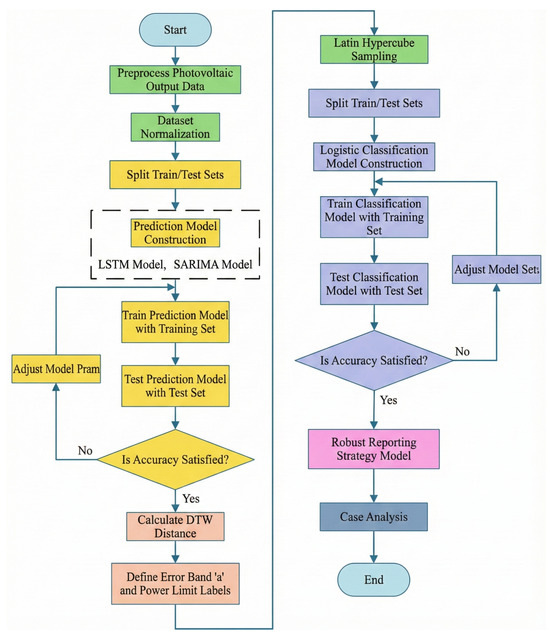
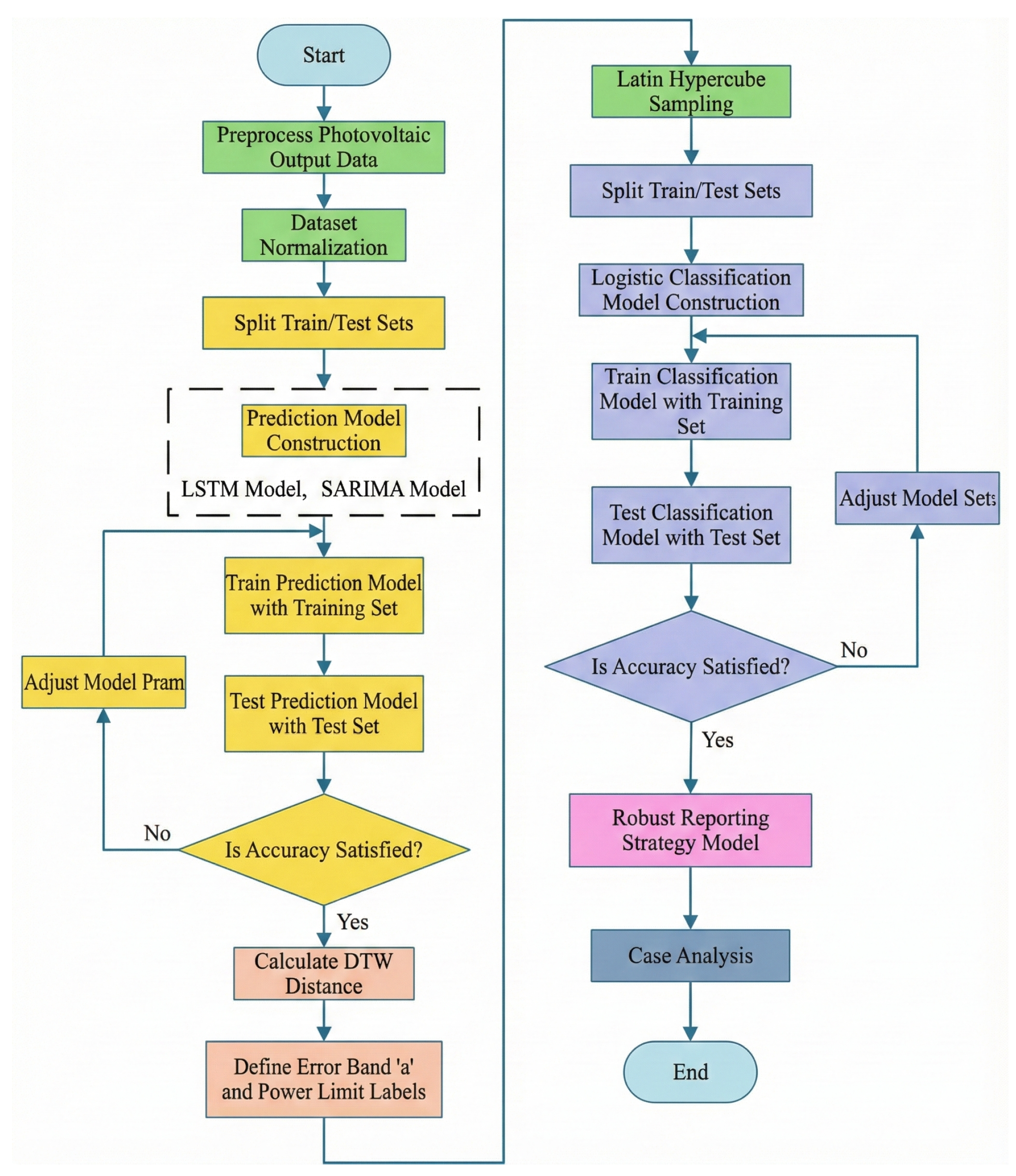
The overall methodology is shown in Figure 1. The framework contains three connected layers. In the physical perception layer, LSTM and SARIMA generate complementary day-ahead forecasts, and DTW extracts the discrepancy between the two forecast trajectories as an uncertainty indicator. In the risk quantification layer, the discrepancy indicator is combined with the candidate error-band width, predicted power, and intra-day time feature to estimate the violation probability through the trained polynomial logistic classifier. In the economic decision layer, PSO searches for the dynamic error-band width that balances bidding aggressiveness and violation risk, and the optimized error band is then passed to the robust bidding model to determine the declared power.
Figure 1.
Overall technical framework of the proposed day-ahead bidding strategy. The optimized dynamic error band obtained from PSO is used as the uncertainty margin in the subsequent robust bidding decision.
The remainder of this paper is organized as follows: Section 2 presents the PV output prediction and dual-model discrepancy quantification method. Section 3 constructs the violation-probability classification model and explains the generation of training labels and input features. Section 4 introduces the dynamic error-band optimization and robust bidding model. Section 5 reports the case study and compares the proposed strategy with fixed error-band benchmarks. Section 6 discusses the limitations and future work, and Section 7 concludes the paper.
2. Comprehensive Model for PV Power Plant Output Prediction
The formulation of the day-ahead bidding strategy begins with the prediction of future output. However, the inherent uncertainty and intermittency of PV output, which are easily affected by weather conditions [18,19], make completely accurate predictions difficult to achieve. Existing research also usually ignores the assessment of predicted power deviation. However, an isolated prediction value cannot inform decision-makers of prediction reliability. To solve this problem, this section introduces dual-model discrepancy analysis, indirectly assessing prediction uncertainty by comparing the prediction results of two models constructed based on different principles.
2.1. Selection of Prediction Models
Considering the nonlinearity and periodicity of PV output data [20,21,22], this paper establishes two prediction models at the PV node: LSTM and SARIMA, defining LSTM as the primary prediction model and SARIMA as the auxiliary prediction model.
LSTM is a Long Short-Term Memory neural network improved based on Recurrent Neural Networks (RNNs) [23]. It solves the “data explosion” and “gradient disappearance” problems in neural network training [24,25], thereby better mining nonlinear relationships in data sequences, making it suitable for scenarios with significant nonlinear characteristics like PV output. The basic unit structure of LSTM is more complex than traditional neural networks, containing forget gates, input gates, and output gates, which realize the forgetting and updating of cell state information through these gating mechanisms.
The SARIMA model is a time-series analysis method suitable for non-stationary data containing seasonal components. It is an extension of the Autoregressive Integrated Moving Average (ARIMA) model [26]. By introducing seasonal components based on ARIMA, this model can effectively describe the periodic fluctuation characteristics existing in PV output data.
2.2. Dynamic Time Warping (DTW)
Dynamic Time Warping is an effective algorithm for measuring the similarity of time series. Addressing the characteristic that PV output is prone to time phase shifts due to weather uncertainty, DTW is not limited to point-to-point rigid matching at each moment but finds the optimal matching path between data in two sequences by adjusting the correspondence between time points. In this study, DTW is used only as a feature for extracting the discrepancy pattern between two forecasts. It is not used to calculate market settlement deviations or penalty quantities, which are still evaluated point by point at each scheduling period. Therefore, DTW provides an uncertainty indicator for the classifier, while the economic assessment remains based on actual temporal deviations between declared and realized power. A smaller DTW distance indicates higher consistency in the evolution trend of the two forecasting sequences.
Assuming that the outputs of the two prediction models are time series of the same length, the primary prediction sequence is and the auxiliary prediction sequence is , with time-series length T. Their expressions are shown in Equations (1) and (2), respectively:
The calculation process of the DTW distance between and is as follows: First, calculate the Euclidean distance between any two time points of the primary prediction sequence and the auxiliary prediction sequence:
where represents the distance between the i-th element of and the j-th element of .
Based on the above calculation, construct a distance matrix :
Based on the distance matrix , the cumulative distance C can be obtained. The recursive formula is as follows:
where represents the minimum cumulative distance from the starting point to , while min represents taking the minimum value of C from the three adjacent units: upper, left, or diagonal.
The boundary conditions for C are
Finally, the DTW distance between sequence and sequence is
3. PV Power Violation Classification Model
By constructing complementary prediction models and employing the DTW algorithm, an indicator capable of dynamically quantifying prediction uncertainty was successfully obtained. However, this difference distance itself is a relative indicator with insufficiently intuitive physical meaning. To establish a bridge between abstract difference distances and specific violation risks, this section transforms this problem into a classification task. A classification model is constructed with known uncertainty information (difference distance) and decisions (error-band width) as inputs, and whether a violation occurs as the output, thereby transforming uncertainty assessment into a probabilistic problem that can guide decision-making.
3.1. Sample Generation for Classification Model
3.1.1. Error Band
Assume that the time series of single-node PV output prediction is expressed as follows:
where is the prediction time domain.
Define the fluctuation upper and lower limits (i.e., error bands) of PV power as the time-indexed ratio . Considering that PV output has strict physical boundaries, i.e., non-negative and not exceeding installed capacity, the error distribution in actual operation often exhibits asymmetric characteristics. Therefore, this paper introduces physical truncation constraints when constructing error bands. The corrected upper and lower bound calculation formulae are as follows:
where represents the upper bound of the error band, represents the lower bound of the error band, and is the installed capacity of the power plant.
For the normalized power values used in the case study, . Therefore, the upper bound of the error band is clipped at 1 p.u., and the lower bound is clipped at 0 p.u. In addition, nighttime and very-low-irradiance periods are masked when constructing violation labels and plotting error bands, because relative errors around near-zero PV output may be numerically unstable and do not represent meaningful bidding risk. The same physical truncation is applied in the revised result figures.
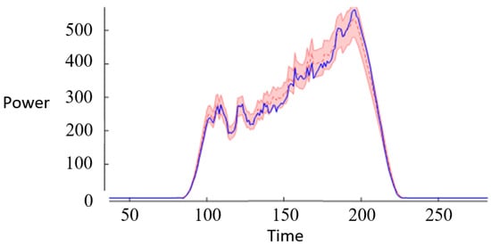
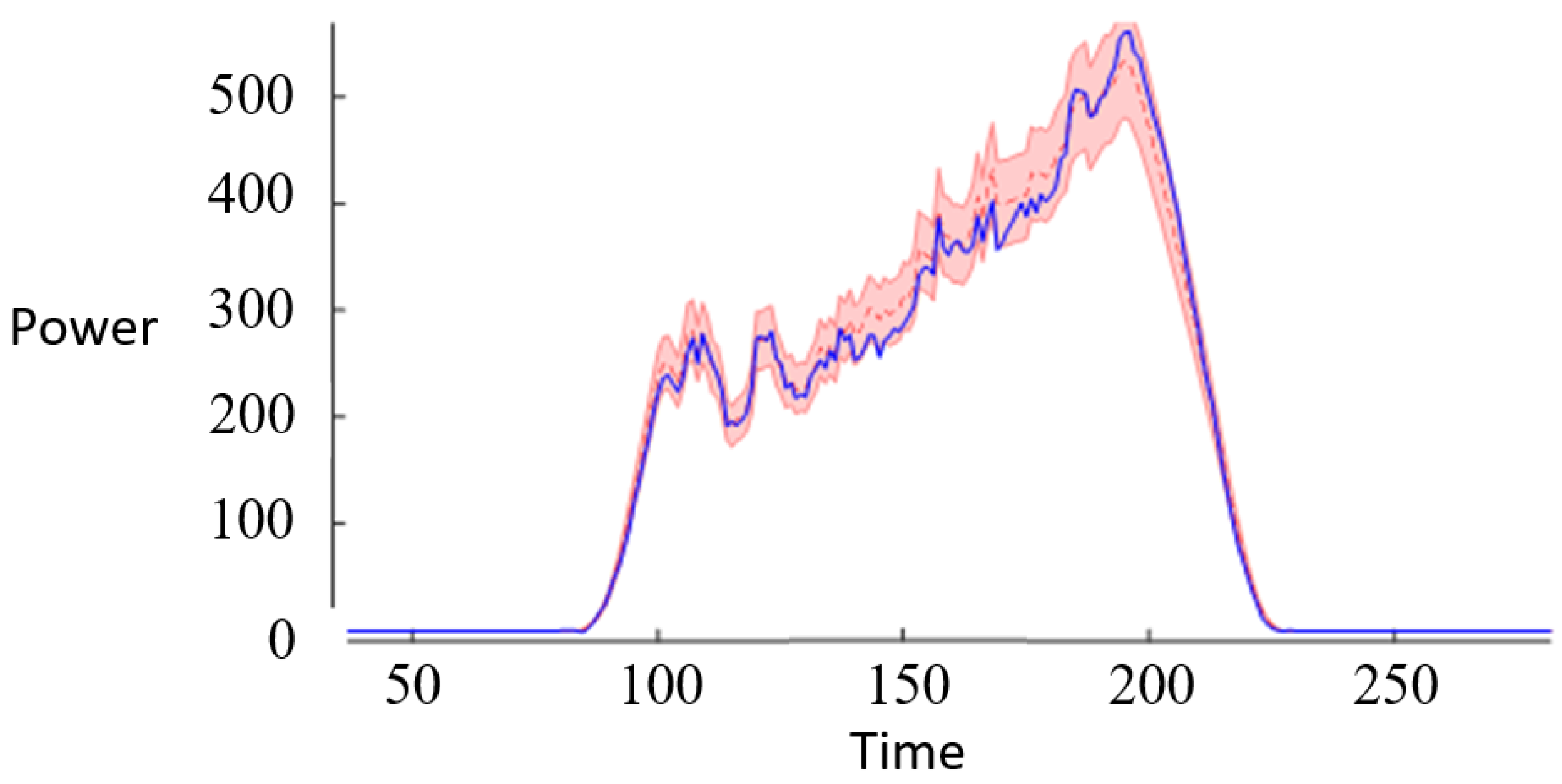
Based on Equations (11) and (12), the violation situation of PV power can be analyzed, and its schematic diagram is shown in Figure 2. The red dashed line represents the predicted power, the upper and lower bounds of the error band constitute the shaded area, and the blue solid line is the actual power. It can be seen that the larger the error band, the larger the shaded area, and the lower the probability of the actual power sequence crossing the boundary.
Figure 2.
Schematic diagram of photovoltaic power violation analysis.
When considering day-ahead bidding for PV power plants, the setting of the error band directly affects the plant’s economics. The error band does not change the physical volatility of PV output; instead, it changes the risk margin used in the bidding decision. A smaller error band usually increases the declared power and potential revenue, but it reduces the tolerance margin and may increase the deviation-penalty risk. A larger error band reduces the probability of violation, but it may cause conservative bidding and revenue loss.
3.1.2. Violation Label
Through training and testing the prediction model with PV operation data, the PV output prediction primary sequence and the actual PV output sequence can be obtained. To avoid the instability of relative errors at night or under extremely low predicted power, the violation-label calculation is performed on the valid daylight set , where is a small power threshold. Define the maximum relative prediction deviation within the considered valid period as
The power violation label is defined as the following binary variable:
where is the i-th element of the actual PV output sequence and is the i-th element of the PV output prediction primary sequence.
When , it indicates that the actual power is out of bounds; when , it indicates no violation. This piecewise definition ensures that the classification label always belongs to , including the boundary case .
3.1.3. Latin Hypercube Sampling
Latin Hypercube Sampling (LHS) [27] is a multi-dimensional parameter space sampling technique extended from traditional Latin square sampling. By establishing a stratified sampling structure within the parameter space, this method ensures that each sample can uniformly cover the entire parameter space, thereby achieving efficient sampling for multi-dimensional variable functions. While maintaining good coverage, LHS can achieve high sampling efficiency with a smaller number of samples.
This paper uses the LHS method to construct training samples, ensuring the randomness of the input variable while making the distribution of the output label y relatively uniform. The classifier is trained offline using historical PV operation data. For each historical prediction period, the historical actual power , the primary predicted power , and the sampled error-band width are used to generate the ground-truth violation label according to the above binary rule. The boundary value is therefore used only in offline historical sample construction. During online day-ahead bidding, future actual PV output is unavailable and is not used; the optimizer only uses forecast information, the dual-model discrepancy, time features, and candidate error-band widths.
First, determine the error-band boundary value according to Equation (15):
Set the sampling interval as , and divide it into N equal-length sub-intervals. The length of each sub-interval is
The i-th sub-interval can be expressed as follows:
where . Randomly select a point in each sub-interval, and after random permutation, constitute the training set of the input variable .
3.2. Classification Model Structure and Training
Based on the input and output sample sets constructed above, to improve the model’s generalization ability under different meteorological scenarios, this paper selects a four-dimensional feature vector composed of prediction difference , error band ratio , predicted power amplitude , and time to noon as the input for the classification model, with the sample label y used as the binary training label. The classifier type is a second-order polynomial logistic regression model with L2 regularization. Its training target is the binary violation state, namely, violation () or no violation (), while its operational output is the violation probability after sigmoid mapping.
The feature denotes the normalized time distance between the current prediction moment and solar noon, rather than a DTW distance calculated around noon. It is introduced because PV output has a clear intra-day pattern: the output is usually higher around noon and lower near sunrise or sunset. This temporal feature helps the classifier distinguish risk patterns at different positions of the daily PV generation curve. It is calculated as follows:
where is the hour of the current time step expressed in decimal form. A smaller indicates that the time step is closer to noon, while a larger value indicates that it is farther from noon.
To capture the complex nonlinear coupling relationship between input variables, this paper selects a polynomial feature mapping model. Since the power violation risk is not linearly determined by a single feature but depends on the dynamic interaction between environmental uncertainty and decision boundaries, introducing polynomial features containing high-order terms and interaction terms can effectively fit this nonlinear risk boundary. Compared with more complex classifiers such as Random Forest and XGBoost, the polynomial logistic model is selected because the feature dimension in this study is relatively low and the second-order interaction terms can explicitly describe the coupling among prediction discrepancy, error-band width, predicted power, and time information. More importantly, logistic regression directly provides a probabilistic output that can be embedded into the subsequent PSO objective function and robust bidding model. Its transparent functional form also helps explain how uncertainty and decision boundaries affect violation risk. The logit expression after second-order feature mapping is as follows:
where are input features, corresponding to respectively; are linear term weights, representing the independent influence of each feature; are quadratic interaction term weights, used to capture the coupling effect between features; and b is the bias term.
The outer layer of the classification model uses the sigmoid function to map the output to a probability value:
The loss function adopts the cross-entropy function:
Due to the high dimension of polynomial function weights, it is easy to cause overfitting. To improve the model’s generalization ability, L2 regularization is introduced to suppress insignificant feature weights. The corresponding loss function is
where is the regularization coefficient.
By training this classification model with historical data, the violation probability corresponding to a candidate bidding boundary can be obtained through the four-dimensional feature vector during actual operation. Specifically, the DTW distance measures the discrepancy between the LSTM and SARIMA forecasts, represents the candidate decision boundary, describes the power level at the current time step, and provides intra-day temporal information. The second-order polynomial logistic regression model maps these features to the probability of violation, which is then used in the subsequent dynamic error-band optimization.
3.3. Classification Model Performance Evaluation Metrics
Since the classification model is used for solving the problem, it is necessary to verify its classification performance to ensure reliability and accuracy in practical applications. This paper divides a portion of the data from the dataset as a test set to evaluate the model’s classification performance. Due to the sparsity of PV power violation events in actual scenarios, the PV dataset samples are unbalanced. Therefore, precision, recall, and F1-score are adopted as the main indicators for measuring the classification performance of the model:
where , , , and represent the number of true positives, false positives, true negatives, and false negatives, respectively.
4. Bidding Decision Model
4.1. Integrated Optimization of Error Band and Violation Probability
This paper employs Particle Swarm Optimization (PSO) to optimize the error-band width and violation probability for each time point. PSO is a global optimization algorithm based on swarm intelligence. Its core idea originates from the simulation of bird flock foraging behavior, utilizing the experience of individuals and the group to search for the optimal solution in the optimization space.
The optimization process of the PSO algorithm includes the following steps:
(1) Initialize Particle Swarm: First, randomly generate a set of particles in the optimization space:
A vector containing all dimensions is used to represent the current position state of the particle, where represents the specific position of the particle in the k-th dimension, and , where n is the dimension of the particle.
Similarly, a vector represents the change direction and step size of the particle, where is the velocity component of the particle in the k-th dimension.
(2) Fitness Evaluation: Evaluate the quality of the current solution for each particle according to the fitness function.
(3) Update Particle Velocity and Position: The velocity and position parameters of the particles are updated according to Equation (27):
where and are the personal best solution and global best solution of the particle, respectively; w is the inertia factor, adjusting the retention degree of the particle velocity, which is related to the global search ability of the algorithm; and are the individual learning factor and group learning factor, respectively, used to adjust the degree of the particle moving towards the individual best and global best; and and are random numbers.
(4) Termination Condition: When the preset stopping condition is met (e.g., the maximum number of iterations or the fitness change is lower than a certain threshold), the algorithm stops and outputs the current optimal solution.
In this study, PSO is applied independently to each scheduling period to obtain the corresponding dynamic error-band width. The population size is set to 20, the maximum number of iterations is set to 100, and the inertia weight decreases linearly from 0.9 to 0.4, so that the algorithm retains stronger global search capability in the early stage and improves local convergence in the later stage. Since the data sampling interval is 15 min, one day contains 96 scheduling periods. Under the maximum iteration setting, each period requires at most fitness-function evaluations, and the daily optimization requires at most fitness-function evaluations. The algorithm stops when the maximum number of iterations is reached or when the change in the fitness value is lower than the preset threshold.
For a given scheduling period t, the LSTM and SARIMA forecasts are first obtained, so , , and are fixed within the PSO optimization of that period. Each particle represents a candidate error-band width . During each iteration, the candidate is combined with the fixed features , , and and fed into the trained second-order polynomial logistic classifier to update the corresponding violation probability . The fitness value is then calculated by Equation (30), and the particle positions are updated until the stopping criterion is satisfied. Therefore, within one prediction period, the DTW distance is precomputed and kept fixed, while the violation probability changes with the candidate value of .
4.1.1. Dataset Construction and Processing
To avoid the influence of dimension and unit differences between different input parameters on model training, data normalization is required. Therefore, the data needs to be normalized, and the output needs to be denormalized after the model training is completed. The normalization and denormalization formulae are shown in Equations (28) and (29), respectively:
where d is the initial data before normalization, is the data after normalization, is the maximum value in the training dataset, and is the minimum value in the training dataset.
4.1.2. Objective Function
The size of the error band directly affects the economics and risk exposure of the bidding decision. In order to integrate bidding aggressiveness and penalty risk before the actual next-day output is known, this study uses a risk-proxy fitness function for each scheduling period. The objective combines the candidate error-band width and the classifier-estimated violation probability :
where and are the weights of the error band size and the violation probability, respectively. The PSO optimization procedure therefore provides the optimized dynamic error band for each scheduling period, which is then used as the uncertainty margin in the subsequent robust bidding model. The realized net revenue is not known during day-ahead optimization and is evaluated afterward in the case study using the settlement model in Section 4.2.
4.2. Robust Optimization Model
In the above content, a PV power violation risk assessment method based on DTW distance and a classification model was proposed. Through the difference analysis of LSTM and SARIMA prediction models, error-band definition, and power violation probability calculation, a framework capable of quantifying PV power uncertainty was initially constructed. On this basis, the optimized dynamic error band obtained from PSO is used to construct the uncertainty set for day-ahead bidding. Thus, PSO and robust bidding are not independent modules: PSO determines the width of the uncertainty interval, and the robust bidding rule converts this interval into the declared power.
Let the PV power plant’s day-ahead bidding output at time t be , the day-ahead predicted output be , and the actual available output the next day be . The uncertainty of the actual output around the forecast is represented by a normalized disturbance variable . To keep the uncertainty set consistent with the physical power bounds, define . Then,
Equivalently, the actual available output is assumed to lie within the dynamic uncertainty interval:
For a PV power plant under a high-penalty assessment mechanism, the conservative day-ahead decision is to maximize the declared power while ensuring feasibility under the worst realization in the uncertainty set:
The worst case for this constraint corresponds to , and the robust counterpart becomes
Therefore, the analytical robust bidding rule is
This expression shows that the final declared power is determined by the optimized dynamic error band from PSO and the forecasted power. The dynamic strategy can be less conservative than a fixed 5% rule in stable periods when , while still enlarging the margin in high-risk periods.
When applying this analytical rule, it is necessary to introduce the actual assessment background of the electricity market as a prerequisite: (1) High Risk of Deviation Assessment: In the current “Two Detailed Rules” assessment, the penalty price caused by power deviation is usually significantly higher than the feed-in tariff. (2) Risk Asymmetry: For PV power plants, the risk weight of direct fine losses caused by actual output being lower than the declared value is much greater than the opportunity cost of abandoned light caused by actual output being higher than the declared value.
This analytical simplification is specific to the assumed penalty structure and risk-asymmetric market context. If the deviation penalty coefficient, allowable deviation rate, or electricity price structure changes significantly, the lower-bound bidding rule may no longer remain optimal. Therefore, the above analytical solution should be interpreted as a robust decision rule under the high-penalty assessment environment considered in this study.
Furthermore, to verify the economic effectiveness of the above bidding decision strategy in actual electricity market settlement, this paper constructs an economic net revenue calculation model containing an allowable deviation domain. Net revenue R is defined as the difference between declared-power settlement revenue and power deviation assessment costs.
First, define the assessed default electricity quantity at time t. When the deviation between actual power and declared power is within the allowable range (), it is exempt from assessment; the excess part needs to pay a fine. The calculation formula is as follows:
On this basis, the daily total net revenue R is expressed as follows:
where T is the number of scheduling periods in the whole day, is the actual available power at time t, is the optimized day-ahead declared power, is the allowable deviation rate, is the PV benchmark feed-in tariff, and is the power deviation assessment penalty coefficient. This indicator will be used in subsequent case studies to quantitatively compare the economic benefits of different strategies.
It should be noted that this revenue model is a simplified settlement model used to compare the relative performance of different error-band strategies. It considers declared-power settlement revenue and deviation penalty costs. Time-varying spot market prices, ancillary service revenue, curtailment costs, transaction costs, operation and maintenance costs, and network constraints are not included in the current formulation.
5. Case Study
The case study data originates from a 20 MW PV power plant in Fujian Province, China. Collected data includes actual output power, solar irradiance, ambient temperature, and wind speed from 1 January 2022 to 1 January 2023, with a sampling interval of 15 min. This one-year record covers seasonal variations within the studied site, but it does not provide multi-year or multi-region validation. Therefore, the geographical and long-term generalization of the proposed strategy is discussed as a limitation in Section 6. The training set accounts for 0.8, and the test set accounts for 0.2. For ease of analysis, the output results of the prediction models in this paper are all normalized values. Operating environment: 13th Gen Intel(R) Core(TM) i7-13650HX processor, 32 GB RAM, Python 3.11.5. The PSO procedure was implemented in Python according to the update equations described in Section 3.1.
Before model training, the input variables are normalized to reduce the influence of different physical units and numerical scales. The data are divided chronologically into training and test sets rather than using random k-fold cross-validation. This is because PV output is a time-dependent sequence, and random shuffling may destroy temporal dependence and introduce information leakage from future samples. Therefore, the chronological split is adopted to better reflect the forecasting and bidding process in practical day-ahead operation.
The specific parameter settings for each model are as follows: (1) The LSTM model contains two LSTM layers, with 64 and 32 neurons, respectively, ReLU activation function, Adam optimizer, learning rate 0.001, and maximum iterations 50. (2) The SARIMA model order is determined by IC criterion, with parameters set to . (3) The PSO algorithm population size is set to 20, maximum iterations 100, and inertia weight w linearly decreases from 0.9 to 0.4. The stopping criterion is reaching the maximum number of iterations or satisfying the preset fitness-change threshold. (4) In the distance calculation of Dynamic Time Warping, the Sakoe–Chiba window is introduced as a global constraint. According to the data sampling frequency, the maximum time offset window (window size) is set to four time steps. (5) The Informer baseline uses the same chronological training and testing split and the same input variables as the other forecasting models. Its result is reported only as a reference baseline under the present dataset and parameter setting, rather than as a general conclusion that Informer is inferior to statistical models or as the main evidence for selecting SARIMA.
5.1. Analysis of Prediction Model Results
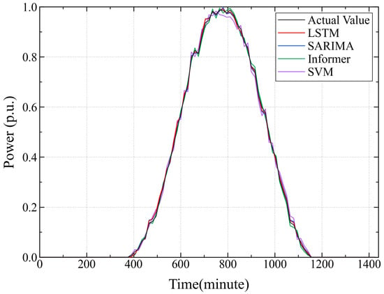
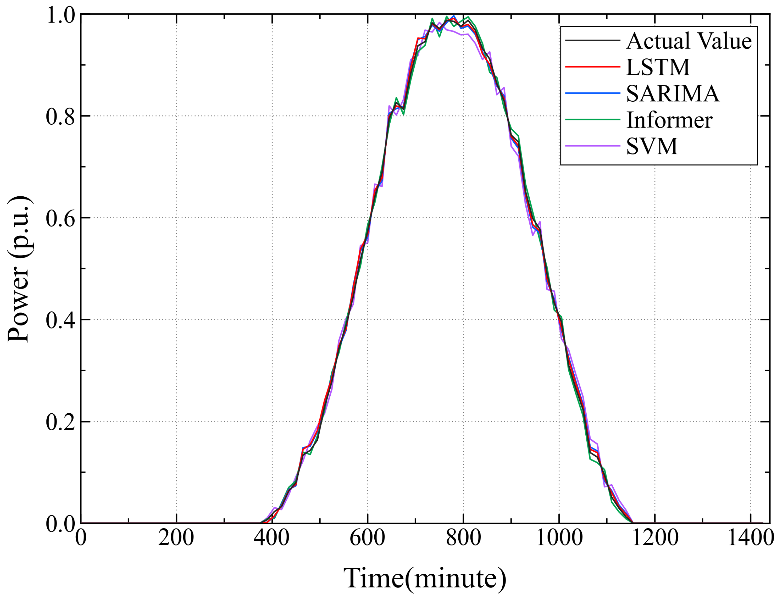
To verify the effectiveness of the selected prediction models, the primary prediction model (LSTM) and auxiliary prediction model (SARIMA) were compared with two other models in terms of performance. The input features of the prediction models include historical power series, irradiance, temperature, and wind speed, and the output is the power value at the future moment. The analysis table of prediction model results based on normalized data and the prediction effect diagram of each model are shown in Table 1 and Figure 3, respectively.
Table 1.
Analysis of forecasting model results with confidence intervals.
Figure 3.
Prediction effect diagrams of various models. The normalized power range is constrained within [0,1] p.u.
Comprehensive analysis of Table 1 and Figure 3 shows that the LSTM model has the best comprehensive prediction performance in this case, with the lowest Mean Squared Error (MSE) and Root-Mean-Square Error (RMSE), and the highest Coefficient of Determination (). The added confidence intervals provide a robustness check for the reported forecasting indicators. They support the conclusion that LSTM performs best under the present test setting, while the intervals of several models still partially overlap; therefore, the comparison is interpreted as a case-specific performance ranking rather than a general statistical dominance claim. The SARIMA model follows closely, with indicators closest to LSTM. The superior performance of the LSTM model lies in its recurrent gating structure. The PV output sequence is affected by multiple complex factors such as irradiance, temperature, and clouds, possessing nonlinearity and non-stationarity. LSTM can effectively learn long-term dependencies and complex nonlinear characteristics in time series, thereby achieving higher prediction accuracy [28,29]. As a classic time-series prediction method, the SARIMA model also performs steadily, and its model interpretability is strong and calculation efficiency is high [30]. The baseline result of Informer should be interpreted cautiously; it reflects the present dataset, input setting, and training configuration, and it does not imply that Informer is generally weaker than SARIMA. In this study, the Informer result is used only as a reference baseline, while SARIMA is selected mainly because it provides a forecasting mechanism complementary to LSTM, which is useful for constructing an interpretable discrepancy-based uncertainty indicator.
5.2. Analysis of Classification Model Results
This study constructed a power violation classification model dataset containing 100,000 samples. This dataset is based on the Latin Hypercube Sampling method, performing combinatorial construction within the parameter space formed by the decision variable and multi-dimensional features () for each prediction time step, producing simulated decision scenarios covering different risk levels.
To verify the rationality of selecting LSTM + SARIMA as the uncertainty quantification indicator, this paper compared the performance of DTW indicators constructed by different model combinations on the risk-identification task. The DTW distances calculated by these three combinations were used as features input to the classifier to evaluate their ability to identify power violation events. The comparison table of risk-identification performance of different dual-model combinations was obtained as shown in Table 2.
Table 2.
Comparison of risk-identification performance of different dual-model combinations.
The results in Table 2 show that the LSTM + SARIMA combination performs best in the risk-identification task considered in this study. The LSTM + Informer combination also uses two data-driven deep-learning models, and its discrepancy feature provides weaker risk-identification performance in the present experiment. This may be related to the relatively similar error structures of the two data-driven models under the current dataset and training setting, but a more detailed error-distribution analysis would be required to draw a general conclusion. Although SVM and LSTM belong to different algorithm categories, SVM’s generalization ability is weaker than that of deep-learning models when capturing the complex temporal dependencies and dynamic evolution laws of PV output. The prediction divergence that it produces may include random model error fluctuations when processing high-dimensional inputs. In contrast, the LSTM + SARIMA combination makes use of the mechanism complementarity of “nonlinear mapping” and “linear statistical laws”. When PV output changes suddenly, the prediction results of the two can show more interpretable divergence, thereby capturing potential uncertainty. Therefore, this combination was selected for constructing the quantitative indicator of the dynamic error band in this study.
Based on the above analysis, this paper selects the LSTM + SARIMA combination to construct the uncertainty indicator. To further verify the statistical validity of this indicator, a correlation analysis was performed on the full amount of data in the test set. The calculated Pearson correlation coefficient between the prediction difference of this combination and the actual prediction absolute error is 0.71, so the two show a significant positive correlation; that is, when the dual-model prediction divergence increases, the actual prediction deviation also increases. This statistical result once again confirms that the DTW distance of the selected combination can effectively characterize the violation risk at the current moment. Based on the optimal combination and verified features, the specific performance evaluation indicators of the classification model on the test set are shown in Table 3.
Table 3.
Performance analysis of the classification model.
Analysis of Table 3 leads to the following conclusions: (1) The total number of samples in the test set is 20,000. Through the balanced sampling of Latin Hypercube Sampling in the parameter space, the number of violation samples was expanded to 1150 (accounting for about 5.75%). Compared with the extremely scarce violation events in the original operation data, LHS sampling not only effectively expanded the sample scale but also significantly alleviated the class imbalance problem caused by the extreme sparsity of power violation events in the original operation data, thereby strengthening the classification model’s ability to identify and capture high-risk scenarios. (2) For non-violation samples, the model’s precision is 0.99, recall is 0.98, and F1 value is 0.98. This indicates that the model has a strong ability to identify normal operating states and can accurately capture the fluctuation characteristics of PV power within the normal range. For violation samples, the model’s precision is 0.96, recall is 0.97, and F1 value is 0.95. Despite the relative scarcity of violation samples, the model can still reach a high performance level, indicating that it maintains good discrimination ability under sparse sample conditions.
It should be clarified that Table 3 evaluates the classifier on the risk-identification sample set constructed from historical periods and LHS-generated error-band scenarios. LHS is used to cover different candidate values of and alleviate the sparsity of violation events, but the chronological train–test split is still preserved to avoid information leakage. To further test whether the classifier relies excessively on the LHS sampling distribution, Table 4 reports the result on a chronological operational test set without LHS rebalancing. The F1-score decreases from 0.95 to 0.88 because the original operational test contains fewer violation samples and stronger temporal imbalance. Nevertheless, the classifier still maintains acceptable precision and recall, indicating that the risk-identification model is not solely dependent on the artificial LHS distribution.
Table 4.
Comparison between the LHS-based risk-identification test and the chronological operational test without LHS rebalancing.
5.3. Analysis of Error Band and Violation Probability Optimization Results
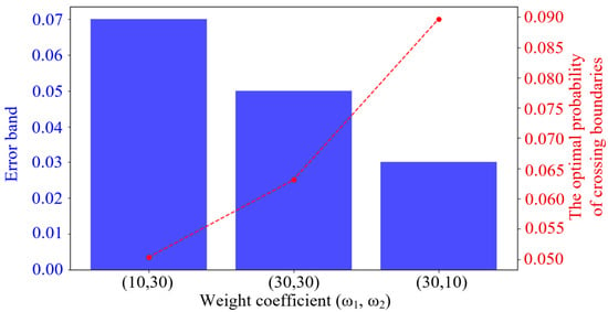
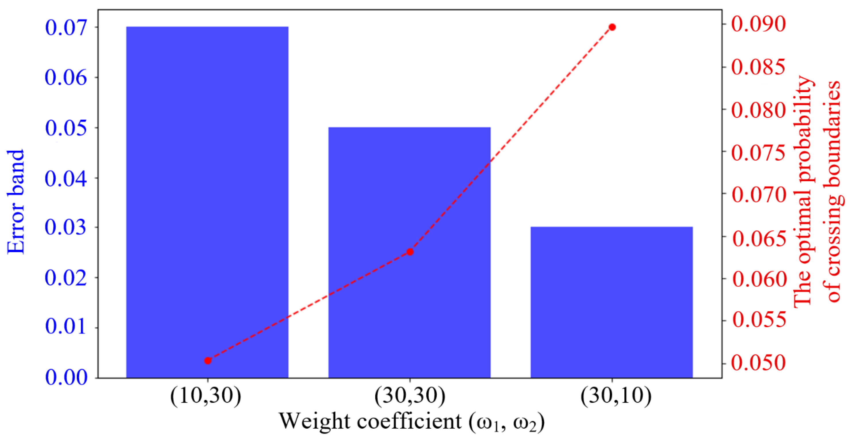
Set different weights for the error band and violation probability, respectively, and solve the model to obtain optimization results under different weights, as shown in Figure 4.
Figure 4.
Optimization results under different weightings.
From Figure 4, it can be seen that when the weight corresponding to the error band is low, the optimized error band is larger and the violation probability is lower, i.e., focusing more on the stability of operation; conversely, when the weight corresponding to the violation probability is low, the optimized error band is smaller and the violation probability is higher, i.e., focusing more on the overall economy. To further quantify the influence of the two weights, a sensitivity analysis is reported in Table 5.
Table 5.
Sensitivity analysis under different weight settings.
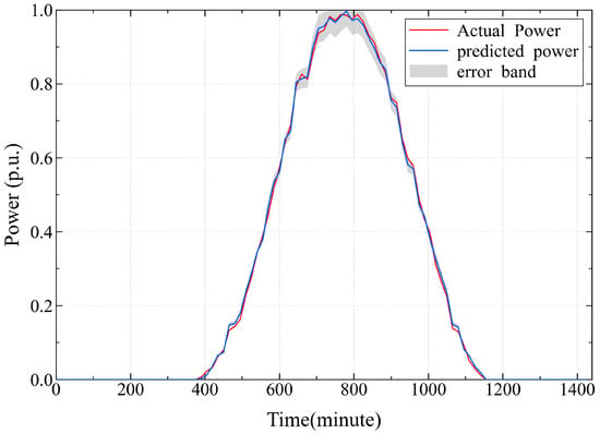
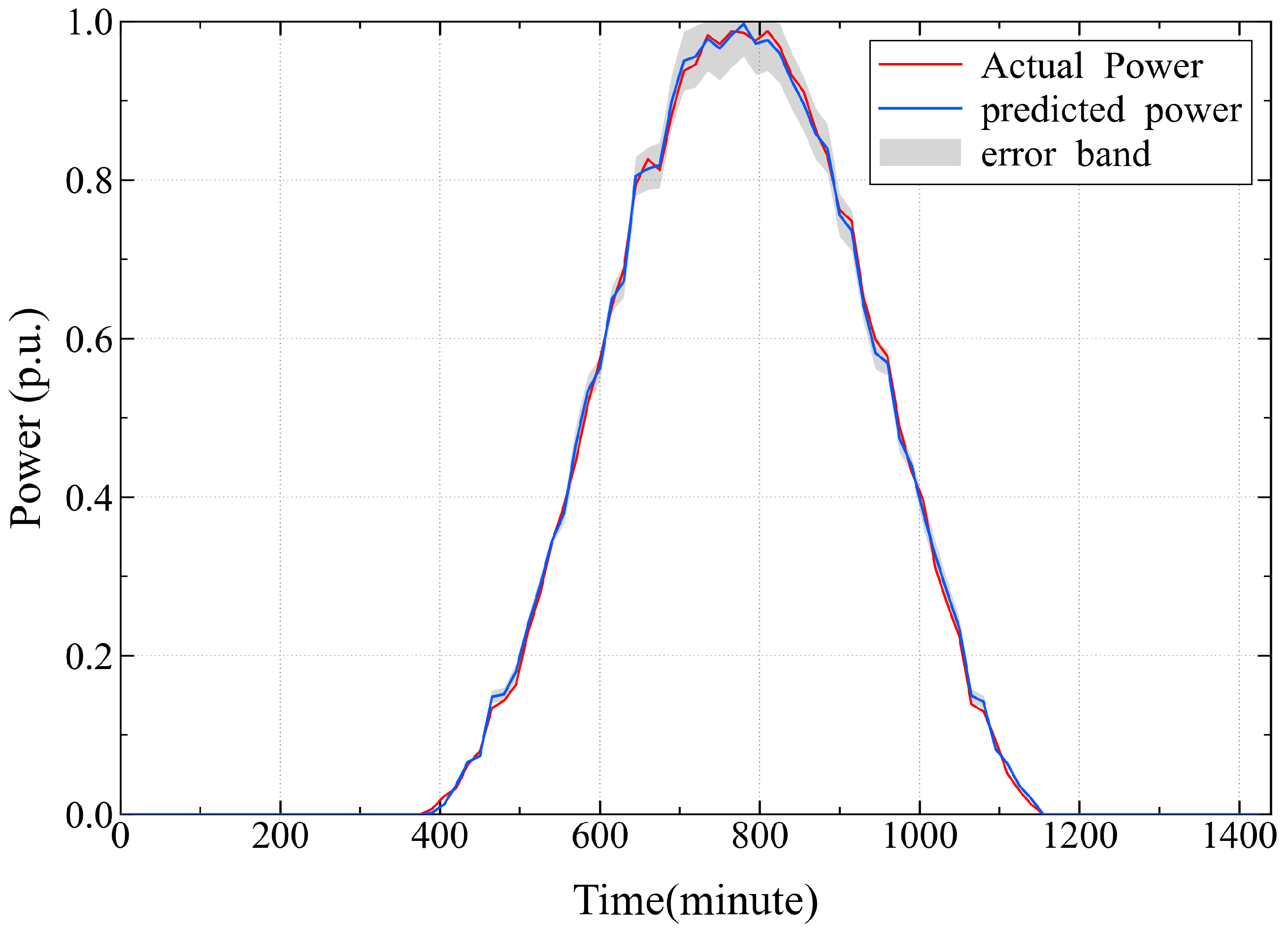
The results show that increasing the weight of the error-band term reduces the optimized band width and increases the declared power, but it also increases the violation probability and the number of violation events. Conversely, increasing the weight of the violation-probability term makes the strategy more conservative. The setting provides the highest net revenue in this comparison while keeping the number of violations at zero. Therefore, Figure 5 shows the optimization result under this balanced weight setting. In the revised figure, the power range and the error-band upper boundary are physically clipped within [0,1] p.u.
Figure 5.
Optimization results at .
5.4. Analysis of Bidding Decision Model Results
To verify the advancement and effectiveness of the dynamic error-band strategy proposed in this paper in the existing PV bidding field, a comparative experiment was set up. Two strategies representing current mainstream engineering decision modes were selected as comparison baselines: a fixed 5% error band, representing an “aggressive” strategy pursuing high bidding volume; and a fixed 10% error band, representing a “conservative” strategy avoiding assessment risks.
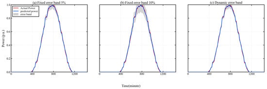
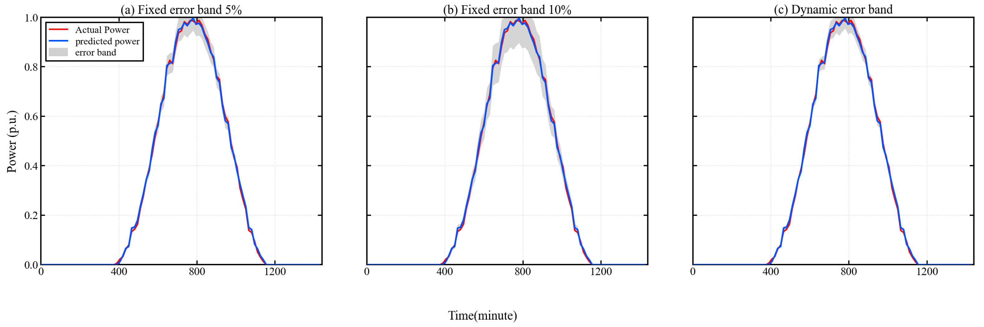
The robust optimization model constructed in this paper aims to establish a decision constraint framework between PV power prediction uncertainty and power station operation economy; on this basis, the PSO algorithm is used to dynamically optimize the error-band width, thereby finding the best balance point between the above two extreme strategies and achieving an effective trade-off between error-band width (economy) and violation probability (security). The experimental results are shown in Figure 6. Figure 6a,b show the optimization results under fixed error bands of 5% and 10%, respectively, and Figure 6c shows the optimization result of the dynamic error band.
Figure 6.
Optimization results under different error-band settings, from left to right: (a) fixed error band 5%, (b) fixed error band 10%, (c) dynamic error band. The upper boundary of each error band is physically clipped at 1 p.u.
To visually quantify the economic benefits of different strategies, this section calculates based on the net revenue evaluation model defined in Section 4.2. According to the latest assessment standards of the Fujian Electricity Market and “Two Detailed Rules”, the case parameters are set as follows: (1) Electricity Price Parameter: The PV benchmark feed-in tariff is set to 0.4 RMB/kWh. (2) Assessment Parameters: The allowable deviation rate is set to 3%; the deviation assessment penalty coefficient is set to 0.6 RMB/kWh to simulate a high-risk assessment environment.
Based on the above parameters, the daily net revenue, total declared power, and violation times under different error-band strategies were statistically analyzed, and the results are shown in Table 6. The same predicted power sequence was used for all three strategies; therefore, the Pred column remains identical. The Bid column differs because each strategy converts the same prediction into declared power using a different error-band margin, namely, after physical truncation.
Table 6.
Statistics of daily power forecasting, violation occurrences, and economic revenue.
Comprehensive analysis of Figure 6 and Table 6 and Table 7 yields the following conclusions: In the case of fixed error bands, when , the PV day-ahead bidding volume is relatively high, at 18.27 p.u., but the number of violations reaches four. The frequent assessment fines resulting from this dragged down the final net revenue to 36,020.5 RMB; when , although the number of violations was reduced to one, the PV day-ahead bidding volume also decreased to 17.31 p.u., losing a large amount of generation revenue due to under-reporting, resulting in a net revenue of only 34,120.2 RMB.
Table 7.
Full-test statistical summary of bidding and revenue indicators.
When using the dynamic error band, the number of violations was reduced to zero, finally achieving a maximum daily net revenue of 37,940.0 RMB. Compared with the robust strategy of a fixed 10% error band, the revenue increased by about 11.2%; compared with the aggressive strategy of a fixed 5% error band, the revenue further increased by 5.3%.
The full-test statistical summary in Table 7 further supports this conclusion. Compared with the fixed 5% and fixed 10% strategies, the dynamic strategy achieves the highest mean net revenue and a lower mean number of violations. The IQR values also indicate that the dynamic strategy maintains a comparable dispersion level while improving the average economic outcome.
Although the design of fixed error bands is simple and easy to implement, it shows obvious limitations in coping with PV output fluctuations. When the fixed error band is set small, although the declared electricity volume can be increased, it easily leads to frequent violation events, increasing the risk of power station assessment penalties; when the fixed error band is set large, although it can effectively reduce the violation probability, it sacrifices economy. In contrast, the dynamic error band realizes the adaptive adjustment of the error-band width through the optimization algorithm. The dynamic strategy does not uniformly adopt a more conservative margin at all time periods. Instead, it can use a narrow margin in low-risk and stable periods, where may be smaller than the fixed 5% benchmark, and enlarge the margin in high-risk periods. Therefore, its total declared power can be higher than both fixed-ratio alternatives while still reducing violation events in the tested daily case.
It should also be noted that Table 6 reports a strategy-level evaluation for the selected daily bidding case, rather than a guarantee of zero violation over the whole year. The zero-violation result indicates that the optimized dynamic margin matched the risk profile of this tested day. More extensive rolling tests under different weather types and market parameters are still needed to evaluate long-term robustness.
6. Discussion
Limitations and Future Work
Although the proposed dynamic error-band optimization strategy improves the balance between economic benefit and violation risk, several limitations should be noted. First, the economic revenue model in this study only considers declared-power settlement revenue and deviation penalty costs. Time-varying spot market prices, ancillary service revenue, curtailment costs, transaction costs, operation and maintenance costs, and network constraints are not included. Second, the proposed uncertainty quantification framework relies on the quality and representativeness of historical PV operation data. Its performance may be affected when the meteorological conditions in the testing period differ significantly from those in the training period. Third, although an additional chronological operational test without LHS rebalancing is reported, the classifier should still be evaluated on more independent continuous operation periods under different weather regimes. Fourth, the robust lower-bound bidding rule is derived under a high-penalty and risk-asymmetric assessment environment. If the penalty coefficient, allowable deviation rate, or market price structure changes significantly, the weight parameters and bidding rule should be re-calibrated. Fifth, the current case study focuses on one PV power plant in Fujian Province and one year of operation data. The one-year dataset covers seasonal variations at the studied site, but it is insufficient to prove multi-year, multi-region, or cross-climate generalization. Sixth, the comparison involving Informer is limited to the present baseline configuration, and further hyperparameter tuning and error-distribution analysis are required for a more comprehensive assessment of advanced deep-learning combinations.
In addition, this study uses a polynomial logistic classification model to maintain probabilistic interpretability and compatibility with the subsequent optimization model. More complex classifiers, such as Random Forest and XGBoost, may further improve nonlinear risk identification in some scenarios, but they require additional comparative evaluation and interpretability analysis. Future research will further incorporate real-time market prices, multi-year and multi-region validation, broader chronological classifier tests, sensitivity analysis under different penalty coefficients and allowable deviation rates, multi-node collaborative optimization, more comprehensive economic settlement mechanisms, and comparative tests of advanced classifiers.
7. Conclusions
Aiming at the uncertainty of PV output in day-ahead bidding, this paper proposes a dynamic error-band bidding framework that links forecast reliability assessment, violation-probability estimation, error-band optimization, and robust declared-power determination. The main conclusions are as follows:
- (1)
- A dual-model discrepancy-based uncertainty quantification method was established by combining LSTM and SARIMA forecasts with DTW distance. The LSTM–SARIMA discrepancy provides an interpretable dynamic indicator for forecast reliability, while the forecasting comparison with confidence intervals supports the case-specific selection of LSTM as the primary predictor and SARIMA as the complementary auxiliary model.
- (2)
- A second-order polynomial logistic regression model was constructed to map the DTW discrepancy, candidate error-band width, predicted power level, and intra-day time feature to violation probability. In addition to the LHS-based validation, the chronological operational test without LHS rebalancing shows that the classifier maintains acceptable risk-identification performance under a more realistic imbalanced temporal distribution.
- (3)
- A PSO-based dynamic error-band optimization strategy was embedded into the robust bidding model. Compared with fixed 5% and fixed 10% error-band strategies, the proposed dynamic strategy reduced the violation events to zero in the selected daily case and increased the net revenue by 5.3% and 11.2%, respectively. The weight-sensitivity analysis and full-test statistical summary further indicate that the dynamic strategy can improve the balance between economic return and violation risk.
It should be noted that the present study is based on one year of data from a 20 MW PV plant in Fujian Province and a specific high-penalty market-assessment setting. Therefore, the conclusions should be interpreted within this case-study scope. Future work will further conduct multi-year and multi-region validation, incorporate real-time market prices and different penalty coefficients, and compare more advanced classifiers and bidding strategies under broader operating conditions.
Author Contributions
Conceptualization, X.H. and K.Y.; methodology, K.Y. and Y.F.; software, K.Y.; validation, X.H., Y.F. and L.W.; formal analysis, K.Y.; investigation, G.Z., Y.L. and Z.Y.; resources, G.Z. and Z.Y.; data curation, K.Y. and Y.L.; writing—original draft preparation, K.Y.; writing—review and editing, X.H., Y.F., L.W., G.Z., Y.L., Z.Y. and K.Y.; visualization, K.Y.; supervision, X.H.; project administration, G.Z.; funding acquisition, X.H. All authors have read and agreed to the published version of the manuscript.
Funding
This research was funded by the Smart Grid National Science and Technology Major Project (2030): Demonstration Project for Multi-Level Coordinated Control of Transmission, Distribution, and Microgrid Systems under High Penetration of Distributed Energy Resources (Grant No. 2025ZD0804600).
Data Availability Statement
The original contributions presented in this study are included in the article. Further inquiries can be directed to the corresponding author.
Acknowledgments
The authors have reviewed and edited the output and take full responsibility for the content of this publication.
Conflicts of Interest
Authors Xinghua Huang, Yuanliang Fan, Lin Wang and Yurun Lin were employed by the State Grid Fujian Electric Power Research Institute. Authors Gonglin Zhang and Zili Yin were employed by the State Grid Fujian Electric Power Co., Ltd. The remaining author declares that the research was conducted in the absence of any commercial or financial relationships that could be construed as a potential conflict of interest.
Abbreviations
The following abbreviations are used in this manuscript:
| PV | Photovoltaic |
| LSTM | Long Short-Term Memory |
| SARIMA | Seasonal Autoregressive Integrated Moving Average |
| DTW | Dynamic Time Warping |
| PSO | Particle Swarm Optimization |
| LHS | Latin Hypercube Sampling |
| SVM | Support Vector Machine |
| CNN | Convolutional Neural Network |
| RMSE | Root-Mean-Square Error |
| MSE | Mean Squared Error |
References
- Zhou, X.; Zhao, Q.; Zhang, Y.; Yang, H.H. Analysis of the Development Trend of China’s Energy and Power System Under the Dual Carbon Target: Green Electricity. Proc. CSEE 2024, 44, 6707–6721. [Google Scholar]
- Wei, H.; Zhuo, Z.; Zhang, N.; Du, E.; Xiao, J.; Wang, P.; Kang, C. Transition Path Optimization and Influencing Factor Analysis of Carbon Emission Peak and Carbon Neutrality for Power System of China. Autom. Electr. Power Syst. 2022, 46, 1–12. [Google Scholar]
- Sun, Z.; Peng, B.; Sun, Y. Optimal dispatch strategy of power and electricity balance based on multi-energy complementation. Electr. Power 2024, 57, 115–122. [Google Scholar]
- Gui, Q.; Xu, W.; Li, X.; Luo, L.; Ye, H.; Wang, Z. Ultra-Short-Term Photovoltaic Power Interval Forecasting Based on Time-Series Decomposition and Conformal Quantile Regression. Electr. Power 2025, 58, 21–32. [Google Scholar]
- Zhou, Y.; Huang, D.; Li, P.; Ji, K.; Liu, X.; Tan, H. A Three-Phase Power Flow Model for Low-Voltage Distribution Networks Considering Balanced Bus Phase Asymmetry and Photovoltaic Access. Electr. Power 2024, 57, 190–198. [Google Scholar]
- Su, H.; Lin, C.; Zhang, Y.; Wang, R.; Cheng, C.; Zhang, J. Regional-level new energy ultra-short-term output prediction method for new energy sources based on Improved AP clustering and dual-attention mechanism. Guangdong Electr. Power 2025, 38, 8–17. [Google Scholar]
- Ye, L.; Pei, M.; Lu, P.; Zhao, J.; He, B. Combination forecasting method of short-term photovoltaic power based on weather classification. Autom. Electr. Power Syst. 2021, 45, 44–54. [Google Scholar]
- Wang, D.; Liu, J.; Huang, Y.; Shi, B.; Jin, M. Photovoltaic power prediction method combinating solar radiation calculation and CNN-LSTM. Acta Energiae Solaris Sin. 2024, 45, 443–450. [Google Scholar]
- Wang, X.; Yu, M.; Ji, M.; Geng, Q.F. Photovoltaic power combination forecasting based on climate similarity and SSA-CNN-LSTM. Acta Energiae Solaris Sin. 2023, 44, 275–283. [Google Scholar]
- Zhang, N.; Ge, L. Photovoltaic system short-term power interval hybrid forecasting method based on seeker optimization algorithm. Acta Energiae Solaris Sin. 2021, 42, 252–259. [Google Scholar]
- Chen, T.; Wang, Y.; Ji, Z. Combination forecasting model of photovoltaic power based on empirical wavelet transform. J. Syst. Simul. 2021, 33, 2627–2635. [Google Scholar]
- Song, S.; Li, B. Short-term forecasting method of photovoltaic power based on LSTM. Renew. Energy Resour. 2021, 39, 594–602. [Google Scholar]
- Wang, K.; Qi, X.; Liu, H. A comparison of day-ahead photovoltaic power forecasting models based on deep learning neural network. Appl. Energy 2019, 251, 113315. [Google Scholar] [CrossRef] [Scilit]
- Wang, K.; Qi, X.; Liu, H. Photovoltaic power forecasting based LSTM-Convolutional Network. Energy 2019, 189, 116225. [Google Scholar] [CrossRef] [Scilit]
- Xu, H.; Mo, R.; Xue, F.; Qin, Z.; Pan, P. Short-term photovoltaic power prediction based on timestamp feature extraction and CatBoost-LSTM Model. Acta Energiae Solaris Sin. 2024, 45, 565–575. [Google Scholar]
- Liu, J.; Lin, S.; Liang, W.; Wang, Q.; Liu, M. Short-term probabilistic forecast for power output of photovoltaic station based on high order markov chain and gaussian mixture model. Power Syst. Technol. 2023, 47, 266–275. [Google Scholar] [CrossRef] [Scilit]
- Wu, Y.; Rong, W.; Guo, Y.; Ye, J. Short-term photovoltaic power forecasting based on SVMD-IDBO-KELM. Acta Energiae Solaris Sin. 2025, 46, 271–279. [Google Scholar]
- Zheng, K.; Wang, L.; Hao, Y. Ultra-short-term prediction of photovoltaic power based on dataset distillation. Proc. CSEE 2024, 44, 5196–5208. [Google Scholar]
- Zhang, T.; Liao, Q.; Tang, F.; Li, Y.; Wang, J.; Deng, H. Wide-area distributed photovoltaic power forecast method based on meteorological resource interpolation and transfer learning. Proc. CSEE 2023, 43, 7929–7940. [Google Scholar]
- Yan, J.; He, W.; Guo, C.; Liu, J.; Li, B.; Li, C.; Zhao, J. Multi-scale photovoltaic power output prediction based on generative adversarial network and Transformer. Electr. Power Autom. Equip. 2025, 45, 25–35. [Google Scholar]
- Cui, Y.; Zhu, H.; Zhang, J.; Wang, M.; Zhao, Y.; Yang, M. Photovoltaic Ultra-short-term Multi-step Power Prediction Based on Satellite Cloud Image and Station Spatial Distribution. Proc. CSEE 2026, 46, 3285–3297. [Google Scholar]
- Deng, F.; Liu, T.; Wang, J.; Gao, B.; Wei, B.; Li, Z. Research on Photovoltaic Power Prediction Based on Multimodal Fusion of Ground Cloud Map and Meteorological Factors. Proc. CSEE 2025, 45, 7193–7206. [Google Scholar]
- Cui, M.; Dong, W.; Lu, Z. CEEMDAN-CNN-LSTM short-term wind power prediction based on density clustering. Mod. Electr. Power 2024, 41, 631–641. [Google Scholar]
- Xu, C.; Xu, Y.; Wang, X.; Meng, Y.; Qin, Y.; Li, W. Research on combined photovoltaic output prediction model based on KPCA, HC and IPSO-LSTM. Acta Energiae Solaris Sin. 2025, 46, 362–374. [Google Scholar]
- Tang, Y.; Chen, X.; Cai, Y.; Yang, Z.; Pu, S.; Yang, C. Tailings dam displacement prediction based on time-series decomposition and SSA-LSTM-Attention model. Sci. Technol. Eng. 2023, 23, 12753–12759. [Google Scholar]
- Valipour, M. Long-term runoff study using SARIMA and ARIMA models in the United States. Meteorol. Appl. 2015, 22, 592–598. [Google Scholar] [CrossRef] [Scilit]
- McKay, M.D.; Beckman, R.J.; Conover, W.J. A comparison of three methods for selecting values of input variables in the analysis of output from a computer code. Technometrics 2000, 42, 55–61. [Google Scholar] [CrossRef] [Scilit]
- Zhang, K.; Ma, L.; Zhang, T.; Zhong, H.; Tan, W.; Wei, Y. Spatio-Temporal Cooperative Probability Forecasting Method for Distributed Photovoltaic Output Based on iDGA-LSTM. Autom. Electr. Power Syst. 2025, 49, 128–138. [Google Scholar]
- Wang, Y.; Cao, Y.; Sun, J. Short-term power load forecasting based on multi-strategy improved golden jackal algorithm-optimized LSTM. Power Syst. Prot. Control 2024, 52, 95–102. [Google Scholar]
- Qin, Y.; Guo, D.; Zhou, F.; Wang, Q.; Wang, Y. Combined SARIMA-GRU-BPNN Model for LTL Logistics Time Series Prediction and Application. Comput. Eng. Appl. 2024, 60, 297–308. [Google Scholar]

Disclaimer/Publisher’s Note: The statements, opinions and data contained in all publications are solely those of the individual author(s) and contributor(s) and not of MDPI and/or the editor(s). MDPI and/or the editor(s) disclaim responsibility for any injury to people or property resulting from any ideas, methods, instructions or products referred to in the content. |
© 2026 by the authors. Licensee MDPI, Basel, Switzerland. This article is an open access article distributed under the terms and conditions of the Creative Commons Attribution (CC BY) license.