Transient Numerical Study of Heat Extraction in Heat Sinks with Sinusoidal Fins Using Perforations

Abstract

The increasing power density of modern electronics demands more efficient thermal management. Heat sinks with sinusoidal fins remain understudied, and the combined effect of perforations and variable fin spacing on transient performance has not been systematically quantified. This numerical study, conducted using ANSYS Fluent 2025 R2, analyzes three sinusoidal fin configurations under forced convection (3–5 m/s): solid fins (Case A), perforated fins (Case B), and perforated fins with alternating spacing of 2 mm and 4.5 mm (Case C). The base was maintained at 60 °C during a 20 s transient period. A mesh with an average skewness of less than 0.25 ensured numerical convergence. Case B showed remarkable uniformity in the base temperature (variations < 1 °C), in contrast to Case A (variations of up to 14.17 °C), due to a thermal boundary layer restart effect induced by the perforations. Case C reached the highest heat dissipation temperatures (up to 54.64 °C at 3 m/s), representing a 47.2% increase compared to Case A, indicating more effective heat extraction with this type of separate fin. The critical transient window occurs within the first 5 s (>85% of the total temperature rise). A vertical temperature gradient of 1.19 °C/mm was observed near the base. Although the perforations reduced the heat transfer area by 5.94%, the induced turbulence compensated for this loss. Sinusoidal fins with perforations and variable spacing significantly improve convective heat removal.

1. Introduction

The advancement of technology, as well as computational processing [1], has progressed by leaps and bounds in recent years; for this reason, electronic devices are tending to get hotter and hotter. For these reasons, it is imperative to improve heat dissipation. The work carried out by Fattahi and Saidi [2] focuses on curved surfaces, concentrating on the air inlet point, investigating the differences between concave and convex constructions.

Microprocessors in computing devices can easily reach temperatures between 80 °C and 100 °C; however, their optimal performance temperature is around 60 °C [3]. Equipment failures due to excessive heating amount to more than 55%. Because of this, there are two cooling methods: direct contact and indirect contact [4]. The techniques for direct contact cooling, the most common ones, are spray cooling [5], forced or natural [6] convective air cooling [7] and jet impingement cooling [8], etc. However, some methods cannot be applied to the cooling of computer systems. On the other hand, various indirect contact techniques can be used. Indirect contact techniques including phase change material cooling [9] and thermoelectric cooling [10] are commonly employed.

Izci et al. [11] carried out a numerical study of the different shapes that a pin fin could have. The shapes varied between circles, rectangles, cones, triangles, rhombuses, and squares. They established that with a sharp-tipped pin fin, this configuration yields the highest heat transfer coefficient due to the occurrence of flow separation. Yaseen et al. [12] numerically analyze various fin shapes, finding that circular fins perform better compared to conical fins. These fins dissipate heat better, evidently due to having a larger surface area, achieving maximum temperatures up to 0.46% lower. Tripathy and Dash [13] in their numerical study of fins for LED cooling, where they used commercial software ANSYS Fluent 2022 R2 under the finite-volume solution method, analyzed eight cases. Among them, they varied the height, length, and number of fins, and found that when the length is greater and the number of fins is also greater, cooling increases. Similarly, in a numerical study using ANSYS, when changing the shape of the fin to a triangular one with grooves, the heat dissipation rate is higher and is improved by 10.44%. However, this does not mean that adding more grooves continues to improve heat transfer [14]. In a comparative numerical study between a heat sink without perforations and one with perforations, the latter provided an improvement of 1.7% in the temperature drop at the tip of the fin with 16 fins, and 3% when the perforation diameter was 1 cm. Likewise, a 1 cm perforation diameter is 1.4% more effective compared to a 0.5 cm diameter for any number of fins; this does not mean that adding more grooves continues to improve heat transfer [15].

When perforations are placed in the fins, although the heat transfer area is reduced, turbulence is increased. The number and shape of the perforations play an important role in the thermal performance of heat sinks [16]. The reduction in cross-sectional area caused by perforations inherently limits the fin’s ability to conduct heat [17]. Despite the unavoidable reduction in fin surface area, circular perforations in plate fins improve heat sink thermal performance by lowering the base plate temperature. The preferred perforation diameters, expressed relative to fin height, were one-fifth and one-tenth—equivalent to 3 mm and 6 mm, respectively, under the conditions examined in ref. [18]. Dastbellaraki et al. [19] developed a numerical study on the thermal performance of perforated fins compared to solid fins. Likewise, they identified that the pressure drop is reduced by increasing the number and size of the perforations. Compared to merely modifying the width of straight channels, the use of a non-uniform wavy mini-channel heat sink is significantly more effective, demonstrating that hindering boundary layer development is indispensable [20]. In another study, two types of heat sinks are used: the first has a horizontal variation in hole size, larger on the left and smaller on the right; the other heat sink has vertically variable diameters, with the smallest at the top and the largest in the bottom. These are compared with a solid heat sink, and it is found that the heat sink with horizontally variable holes shows an improvement in the heat transfer coefficient of close to 23% [21].

This research focuses on a numerical study, using the commercial software ANSYS Fluent, of heat dissipation through a heat sink with sinusoidal fins. Various aspects were varied, such as the inlet velocity, which ranged from 3 m/s to 5 m/s. These velocities correspond to forced convection heat transfer. Furthermore, this study is extended by incorporating perforations in the heat sink fins. Although this reduces the heat transfer area, the resulting turbulence is likely to contribute to a temperature reduction in the heat sink.

2. Materials and Methods

2.1. Geometry

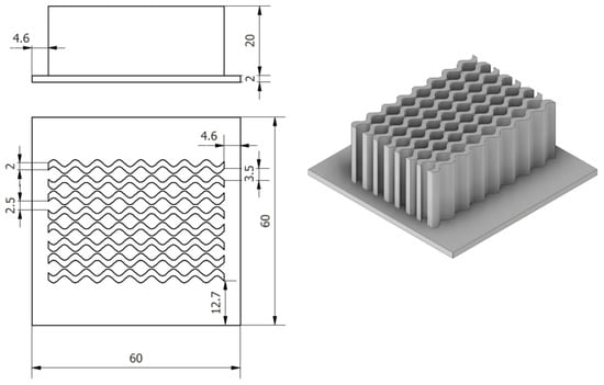
Heat sinks can have any type of geometry, with rectangular fins being among the most typical. However, curved-profile fins have not been as extensively studied. For this study, a heat sink with eight identical fins following a sinusoidal distribution was designed. This profile was constructed using parametric equations, which allowed for precise control of the amplitude and frequency of the undulation, ensuring uniformity throughout the dissipation channel.

Figure 1 shows the model of the heat sink with sinusoidal curved fins.

Figure 1. Heat sink with sinusoidal curved-profile fins.

As mentioned, the study focuses not only on a single type of heat sink but on three heat sinks with sinusoidal curved fins. However, there are fundamental differences in the heat sinks, such as holes along the fin height.

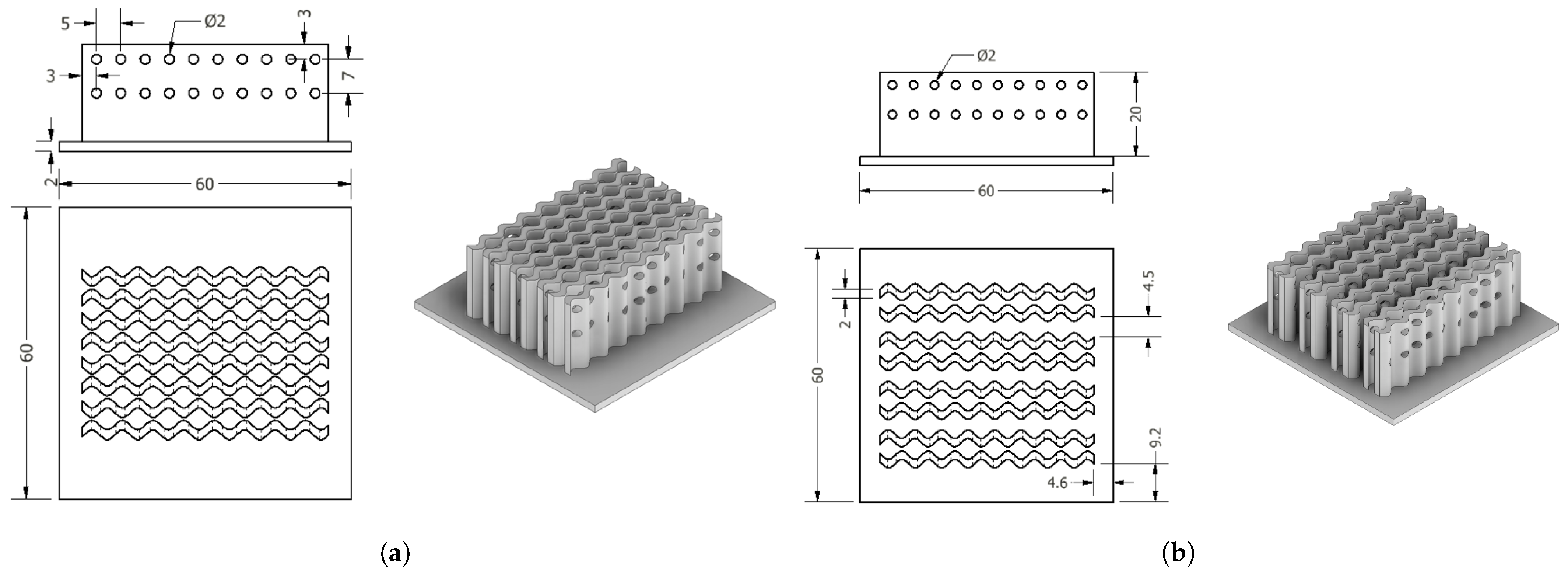
Figure 2 shows a representation of the heat sink with holes; there are 20 holes per sinusoidal fin. The hole diameter is 2 mm, with a horizontal spacing of 5 mm and a vertical spacing of 7 mm between holes. This configuration reduces the heat transfer area by 5.94% between these two cases. Figure 2b shows the heat sink with an inter-fin spacing of 4.5 mm; however, this is not a consistent pattern across all fins. This spacing is present every two fins, while the initial 2 mm spacing is maintained between the other fins. In this case, the heat transfer area is the same as in case 2, shown in Figure 2a. A diameter of 2 mm is a practical size that can be reliably produced using both additive manufacturing (3D printing) and CNC machining. A horizontal spacing of 5 mm ensures that the holes are sufficiently far apart to prevent stress concentration zones that could lead to deformation or failure under thermal and mechanical loads. The 7 mm vertical spacing ensures that the holes are distributed along the height of the fin without creating weak planes that could compromise structural performance; this value was selected to preserve the overall stiffness of the fin structure while allowing for adequate flow mixing and improved heat transfer.

Figure 2. Heat sink with sinusoidal curved-profile fins: (a) Circular perforations. (b) Circular perforations with fin-to-fin amplitude.

2.2. Materials and Mesh

All simulations for the three heat sink scenarios described were performed using the commercial CFD software ANSYS Fluent 2025 R2. To ensure that this numerical study closely resembled real conditions, the three heat sinks were made of aluminum. Although aluminum does not have as high a thermal conductivity as other materials, its low density makes the heat sinks lighter. Based on this premise, the heat transfer areas can be extended without significantly increasing the weights of the heat sinks.

Table 1 shows the physical and thermal properties of both the heat sink material and the air flowing through it. Furthermore, it is essential to clarify that the air inlet temperature is 18 °C, and the air velocities range from 3 m/s to 5 m/s.

Table 1. Thermal and physical properties of the heat sink and the surrounding air [22].

Properties	Aluminum	Air (18 °C)	Unit
Density	2719	1.212	kg·m−3
Specific heat Cp	871	1007	J·kg−1·K−1
Thermal conductivity	202.4	0.02498	W·m−1·K−1
Viscosity	-	1.8158 × 10−5	kg·m−1·s−2

Although the heat sinks are different from traditional ones, they share physical spaces with conventional heat sinks. The lower parts of these devices are what receives heat directly; from there, dissipation begins, in some cases with rectangular fins, in others with curved ones. Since this study was carried out using CFD, it was important to create a mesh of the geometry to establish the finite volumes and also to set the boundary conditions.

When analyzing the heat sink geometry, it has already been mentioned that they feature sinusoidal fins, eight in total, with and without perforations. The base plates have dimensions of 60 mm, 60 mm, and 2 mm in width. On the other hand, the fin height is 20 mm, with a heat transfer area per solid fin of 2573.178 mm² and per fin with holes of 2420.146 mm².

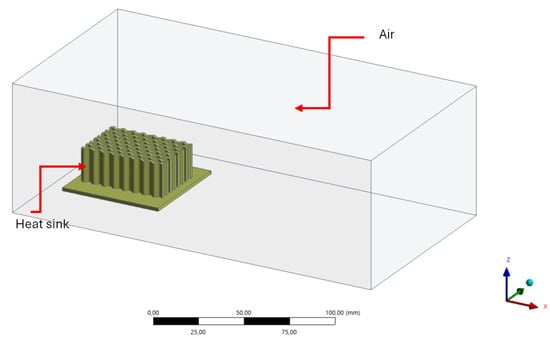
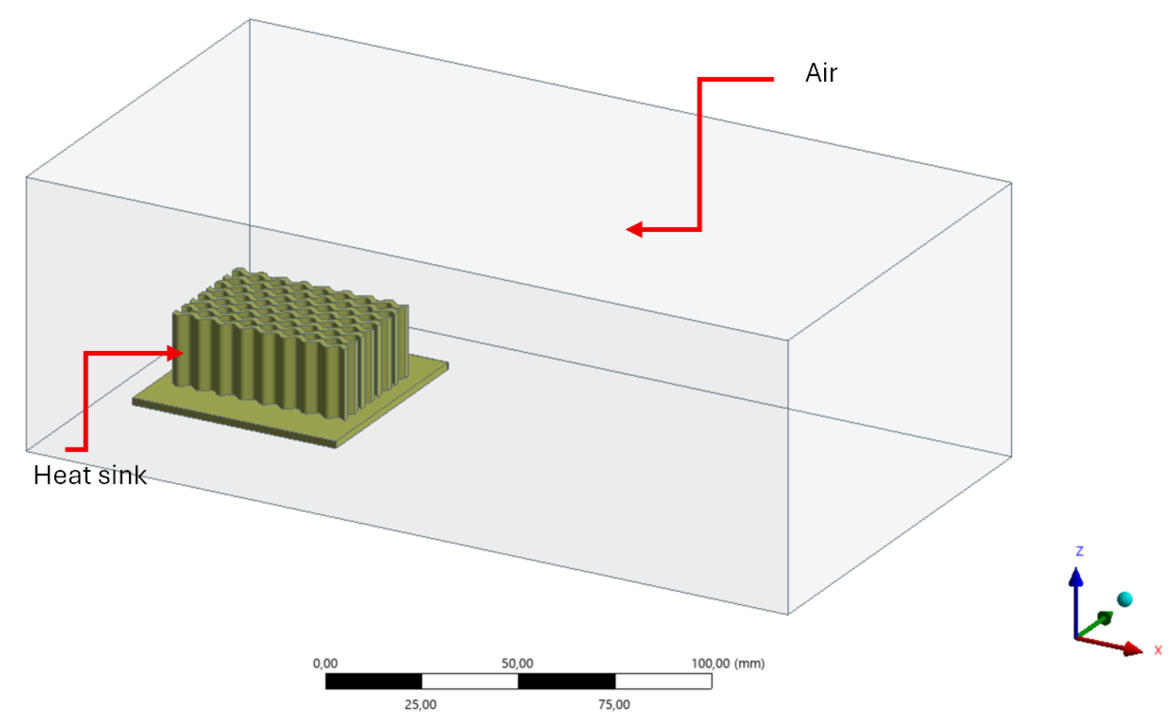
Figure 3 shows the heat sink at the center of an air structure. This enclosure simulates the air around the heat sink; however, the dimensions are not symmetric—it was necessary to have more air space after the surfaces of the device. Therefore, the following distances for the air volume were established: +x 150 mm, −x 15 mm, +y 30 mm, −y 30 mm, +z 50 mm, and −z 5 mm.

Figure 3. Air enclosure around a heat sink.

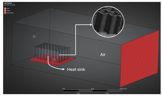
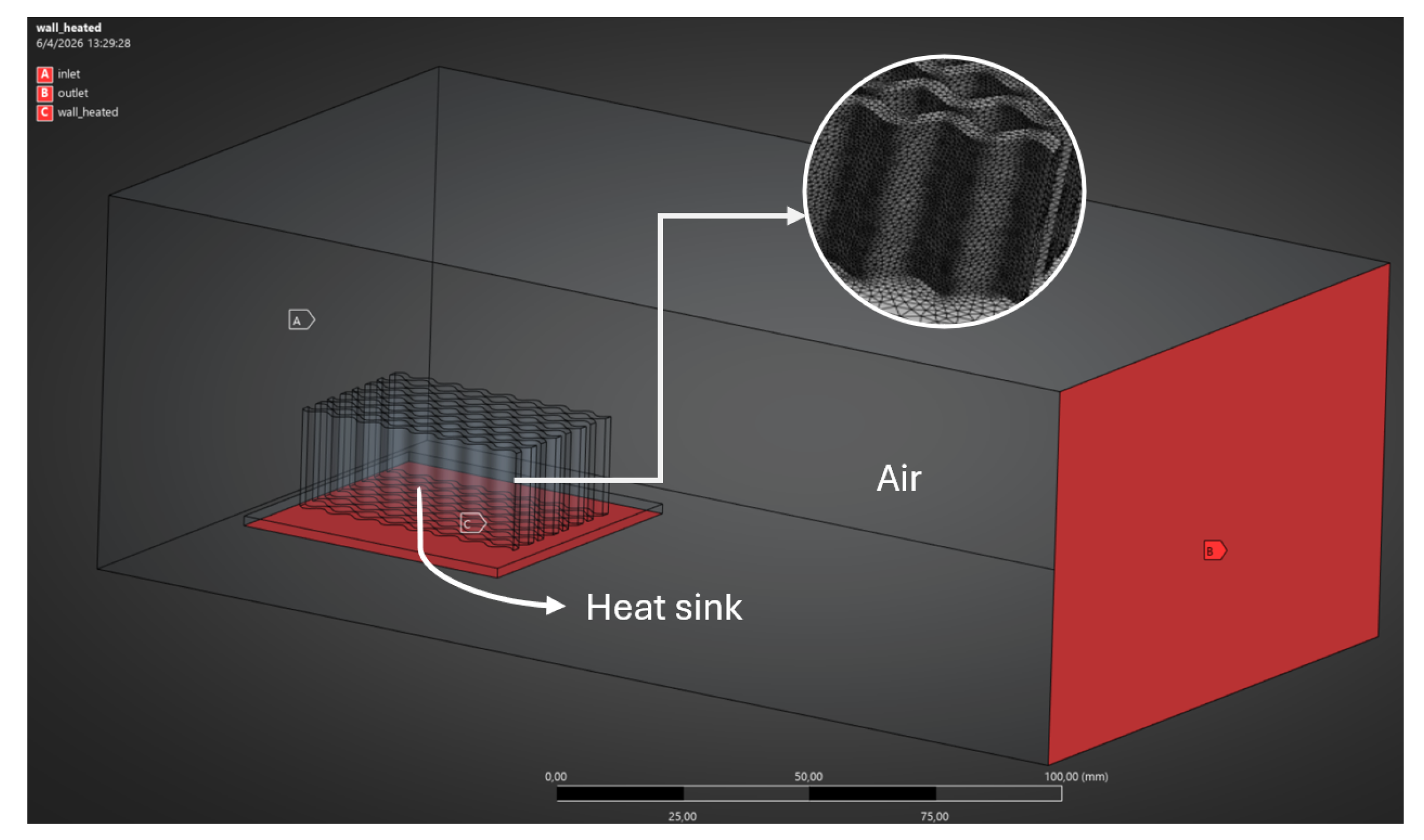
As this is a numerical simulation using CFD, it is necessary to generate a structured mesh of the domains to be analyzed. In this case, these domains are the heat sinks with sinusoidal curved fins and the surrounding air. Figure 4 shows the mesh of a heat sink, as well as the air inlet and outlet, along with the wall that receives the heat coming from the electronic device.

Figure 4. Boundary conditions applied in the simulation of a heat sink.

Markers A, B, and C represent the inlet, outlet, and hot wall, respectively. On the other hand, the mesh in the heat sink section is relatively small compared to the surrounding air. This is because the process will take place on the fins of the heat sink.

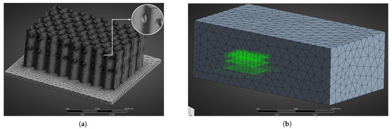
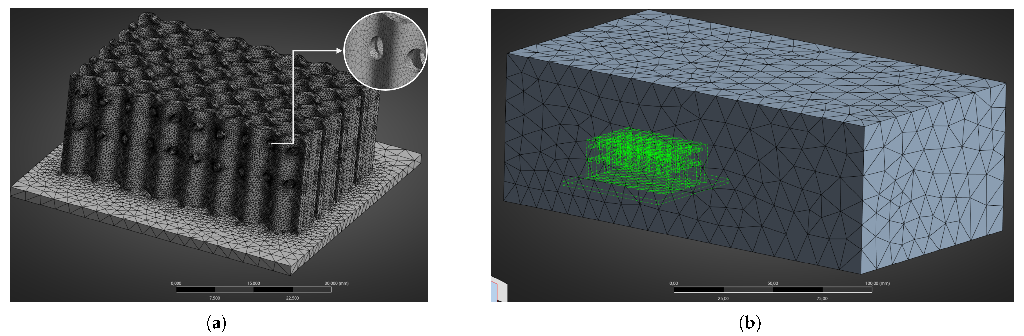
It is also extremely important to define a mesh for the fins when they have holes. This is why, in Figure 5, it can be seen how the mesh becomes finer as it approaches the holes in the fins. The mesh of the air region is the same for all simulations. Figure 5b shows the external mesh of the surrounding air.

Figure 5. Mesh of the heat sink and surrounding air: (a) Mesh refinement on the heat sink featuring holes in the fin profile. (b) Mesh of the air surrounding the heat sink.

Reemphasizing the importance and necessity of analyzing the mesh in the simulations to be performed, different values were obtained for the number of nodes and elements present in each simulation case. In agreement with various CFD studies that employ the skewness method, this refers to an asymmetry criterion that determines how close a face or cell is to the ideal shape (i.e., equilateral or equiangular). A value of 0 corresponds to an equilateral mesh, while a value of 1 corresponds to a degenerate mesh. Intermediate values also satisfy several simulation conditions, since when the value is less than 0.25, the model is considered excellent, while between 0.25 and 0.5, it is considered good [23].

The number of nodes and cells in each simulation varies, as Case A consists of a heat sink with curved fins, Case B features the same heat sink geometry with the addition of perforations (holes), and Case C incorporates both the fin spacing modification and the perforations identical to those in Case B. Table 2 presents the node and element count for each configuration, along with the average skewness metric. All cases exhibit an average skewness value below 0.25, which is indicative of a high-quality (excellent) mesh. In addition, preliminary simulations were conducted to minimize mesh size errors, striking a balance between the number of elements and the relative error in the results.

Table 2. Mesh node and element distribution per simulation case for each heat sink model.

Simulation	Nodes	Elements	Skewness Average
Case A	559,242	3,335,967	0.2383
Case B	750,716	4,482,627	0.2357
Case C	828,802	4,938,819	0.2423

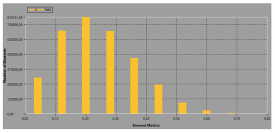
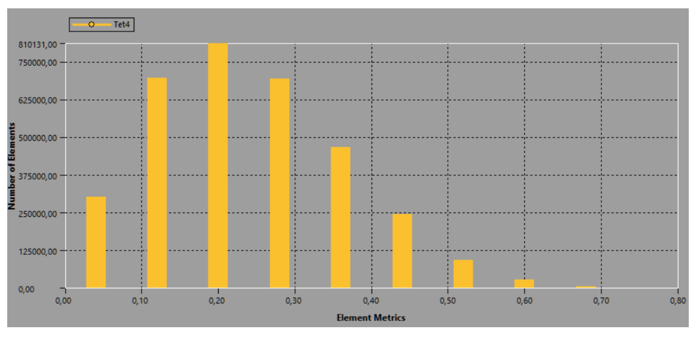
Figure 6 illustrates the sectorization of element quality based on the skewness metric. It is observed that the predominant portion of the mesh population lies within the interval from 0 to 0.5. Furthermore, a significant majority exceeding 50% of the total element count is clustered in the sub-interval reaching up to 0.25. This clustering provides strong evidence of adequate mesh convergence, thereby validating the integrity and accuracy of the subsequent computational results.

Figure 6. Element count versus average skewness distribution for the evaluated geometries.

2.3. Governing Equations

The classical governing equations of fluid mechanics and heat transfer remain entirely applicable to the present study. Nevertheless, their coupling with computational fluid dynamics (CFD) is required. Within the CFD framework, three fundamental conservation equations are considered: the conservation of energy, the conservation of momentum, and the conservation of mass. The heat transfer in the airflow is modeled using the mass, momentum, and energy conservation equations written below [24]:

$${\displaystyle \frac{\partial \rho }{\partial t}}+\nabla ·\left(\rho \overrightarrow{v}\right)=S_m$$

(1)

$${\displaystyle \frac{\partial }{\partial t}}\left(\rho \overrightarrow{v}\right)+\nabla ·\left(\rho \overrightarrow{v}\overrightarrow{v}\right)=-\nabla p+\nabla ·\left(\stackrel{=}{\tau }\right)+\rho \overrightarrow{g}+\overrightarrow{F}$$

(2)

The stress tensor $\stackrel{=}{\tau }$ is given by

$$\stackrel{=}{\tau }=\mu \left[\left(\nabla \overrightarrow{v}+\nabla {\overrightarrow{v}}^T\right)-{\displaystyle \frac{2}{3}}\nabla ·\overrightarrow{v}I\right]$$

(3)

$${\displaystyle \frac{\partial }{\partial t}}\left(\rho E\right)+\nabla ·\left(\overrightarrow{v}\left(\rho E+p\right)\right)=-\nabla ·\left(\sum _j{h}_j{J}_j\right)+S_h$$

(4)

$$E=e+{\displaystyle \frac{1}{2}}{\left|\overrightarrow{v}\right|}^2$$

(5)

The simultaneous solution of two transport equations within two-equation turbulence models yields both a turbulent length scale and a turbulent time scale. Within this framework, the $\kappa -ϵ$ model is recognized as exceptionally robust and well-suited to the simulations conducted herein. The turbulence kinetic energy, $\kappa$, and its rate of dissipation, $ϵ$, are obtained from the following transport equations:

$${\displaystyle \frac{\partial }{\partial t}}\left(\rho k\right)+{\displaystyle \frac{\partial }{\partial x_i}}\left(\rho k{u}_i\right)={\displaystyle \frac{\partial }{\partial x_j}}\left[\left(\mu +{\displaystyle \frac{{\mu }_t}{{\sigma }_k}}\right){\displaystyle \frac{\partial k}{\partial x_j}}\right]+G_k+G_b-\rho \epsilon -Y_M+S_k$$

(6)

and

$${\displaystyle \frac{\partial }{\partial t}}\left(\rho \epsilon \right)+{\displaystyle \frac{\partial }{\partial x_i}}\left(\rho \epsilon u_i\right)={\displaystyle \frac{\partial }{\partial x_j}}\left[\left(\mu +{\displaystyle \frac{{\mu }_t}{{\sigma }_{\epsilon }}}\right){\displaystyle \frac{\partial \epsilon }{\partial x_j}}\right]+C_{1\epsilon }{\displaystyle \frac{\epsilon }{k}}\left(G_k+C_{3\epsilon }{G}_b\right)-C_{2\epsilon }\rho {\displaystyle \frac{{\epsilon }^2}{k}}+S_{\epsilon }$$

(7)

The turbulent (or eddy) viscosity ${\mu }_t$ is calculated as

$${\mu }_t=\rho C_{\mu }{\displaystyle \frac{k^2}{\mathcal{E}}}$$

(8)

In these equations, $G_k$ represents the generation of turbulence kinetic energy due to the mean velocity gradients. $G_b$ is the generation of turbulence kinetic energy due to buoyancy. $Y_M$ represents the contribution of the fluctuating dilatation in compressible turbulence. $C_{1\epsilon }$, $C_{2\epsilon }$, and $C_{3\epsilon }$ are the turbulent Prandtl numbers for k and E, respectively [24].

It is well known that Fourier’s law describes the constitutive relation linking the heat flux to the temperature gradient in a fluid [25,26], which can be written as

$$\overrightarrow{q}=-k\nabla T$$

(9)

where $\overrightarrow{q}$ denotes the heat flux circulating through any point in the fluid, also reflecting the fluid’s ability to transfer heat by convection. Meanwhile, k is the thermal conductivity of the material, and T represents the temperature variation between the surfaces being analyzed.

On the other hand, the heat transfer by conduction from an internal wall to the fin surface is given by [27]

$$q={\displaystyle \frac{k(T_w-T_{fin})}{L}}$$

(10)

The heat transfer equations for heat dissipation using this type of element include both conduction, as previously discussed, and also external forced convection, which accounts for a portion of the heat transfer. The Nusselt equation is used to determine the heat transfer coefficient of the external air surrounding the heat sink [28].

$$N{u}_x=0.0296R{e}_x^{4/5}P{r}^{1/3}$$

(11)

3. Results

CFD simulations are versatile and easy to set up. However, this depends heavily on the methods and models used to solve the problem. After defining the mesh and boundary conditions, data processing and post-processing must be performed. For data processing, it is essential to incorporate the energy and turbulence equations along with the specific values into the discretization.

For the boundary conditions, there are three defined cases regarding the inlet velocity, which flows through the entire heat sink longitudinally, parallel to the “x” axis. These velocities are 3 m/s, 4 m/s, and 5 m/s; on average, these are the velocities generated by the fans in forced convection [29,30].

It is important to note that there will be a constant value at the base of the heat sink in all cases; this value is 60 °C. Furthermore, these speed and temperature conditions will apply to all three types of heat sinks: the sinusoidal-fin heat sink, the heat sink with holes, and the heat sink with separate fins and perforations.

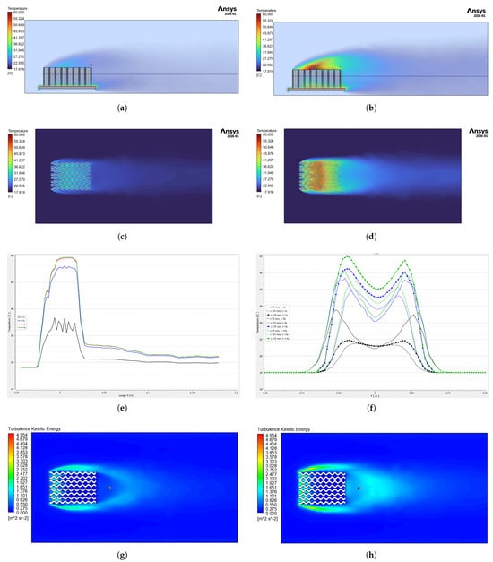
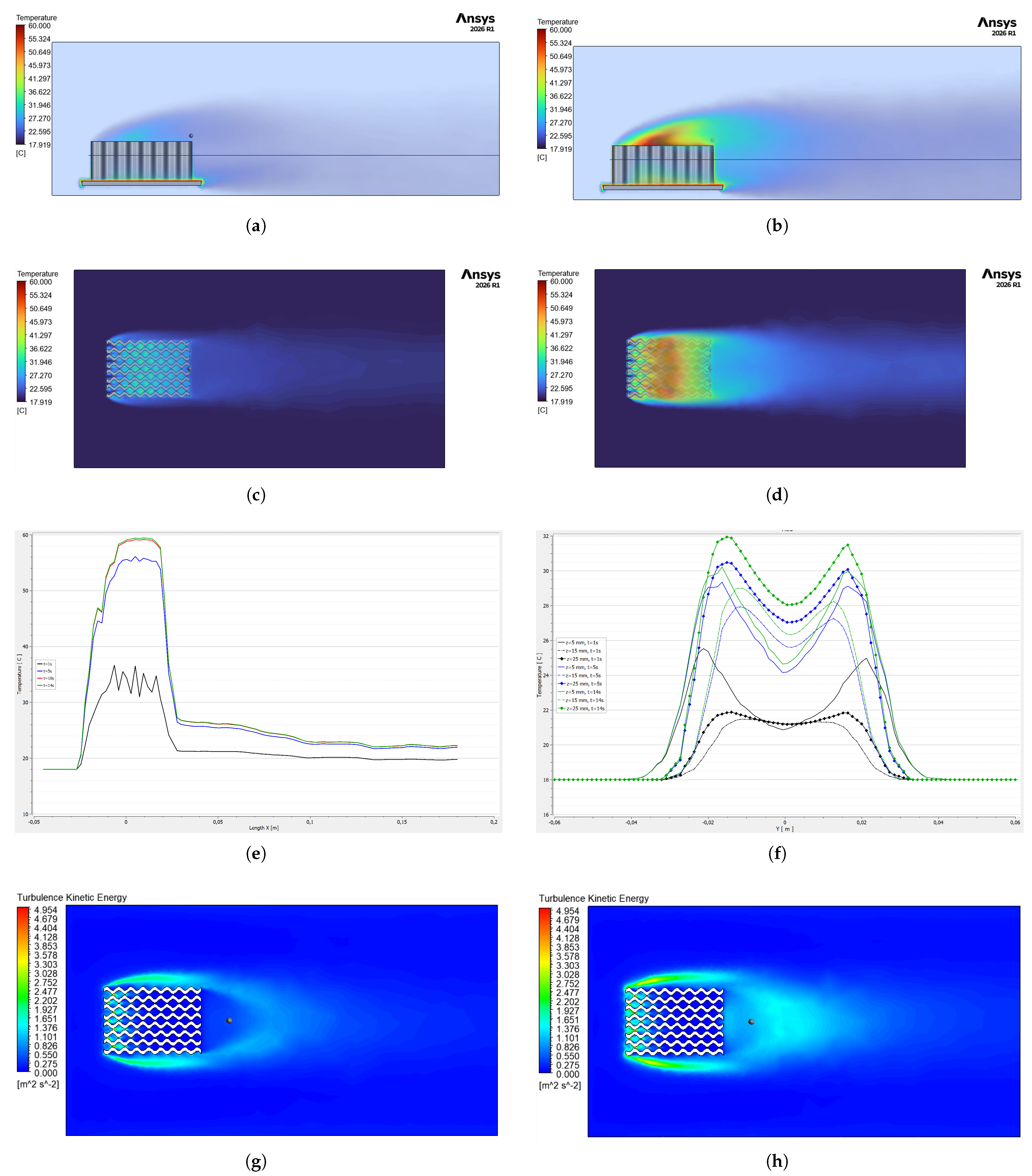
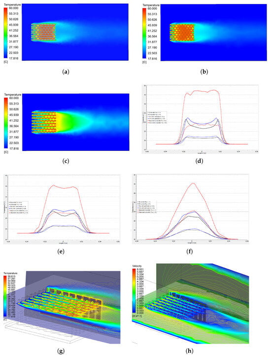
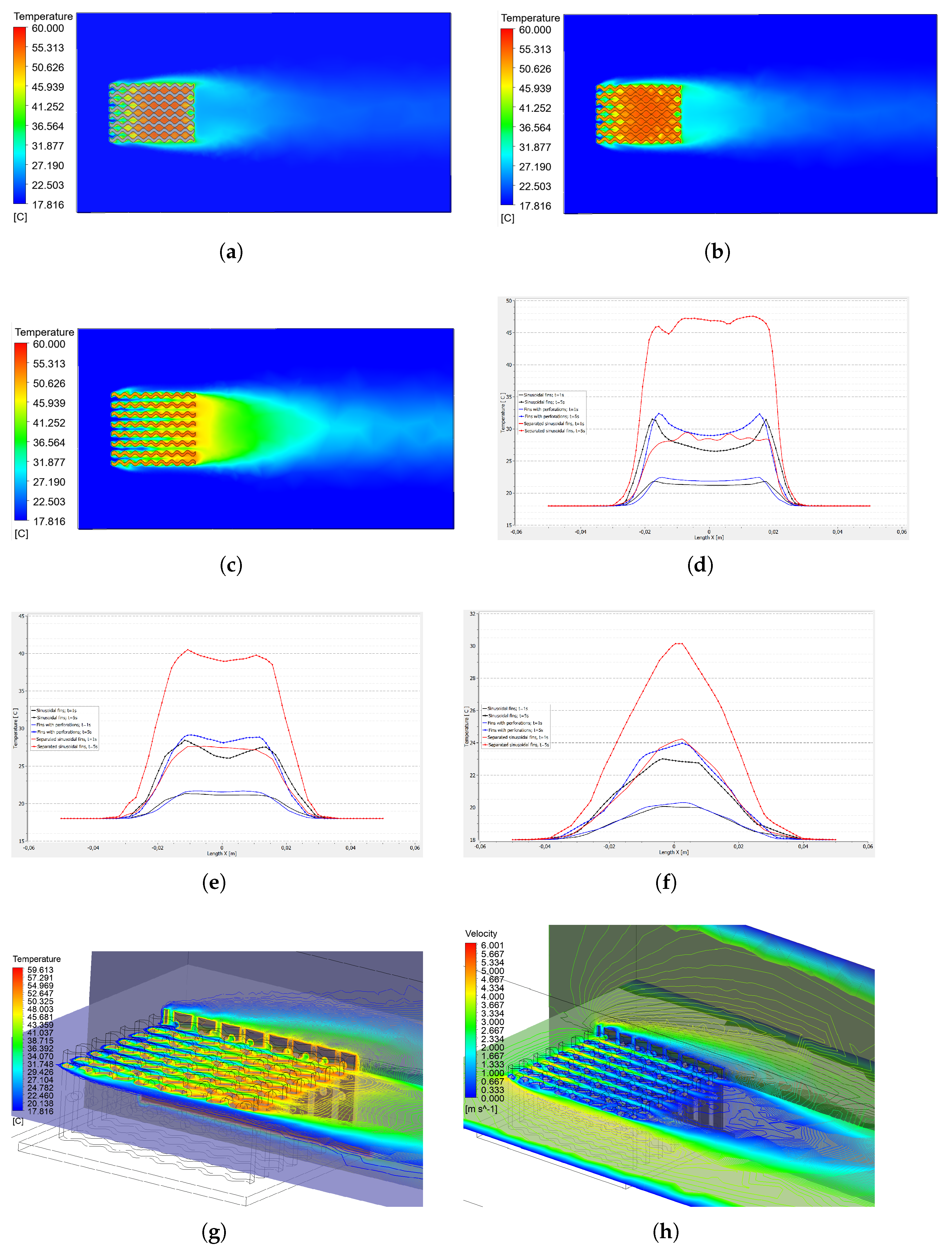
Figure 7 illustrates heat dissipation through the system, featuring a heat sink with sinusoidal fins and no perforations. The figure displays various aspects of the simulation, including flow rates, temperature contours, and temperature distribution profiles at various points on the heat sink and in the surrounding air.

Figure 7. Heat sink with sinusoidal fins, velocity of 3 m/s: (a) Side view of heat dissipation at 1 s. (b) Side view of heat dissipation at 10 s. (c) Temperature contour at 1 s. (d) Temperature contour at 10 s. (e) Temperature distribution along the line on the x-axis. (f) Temperature distribution at 3 height levels on the z-axis. (g) Turbulence kinetic energy in the base heat sink. (h) Turbulence kinetic energy in the perforated heat sink.

Figure 7a shows a side view of the heat sink at a velocity of 3 m/s and a base temperature of 60 °C; however, these simulations are in a transient state, so at the 1 s mark, the maximum air temperature is 29.71 °C. On the other hand, Figure 7b shows the side view again, this time at 10 s; in this case, the temperature has reached 57.77 °C. In another simulation at 14 s, the temperature has risen to 58.08 °C. In the first case, there is an increase in air temperature of 28.06 °C over the 9 s interval. However, the temperature change from 10 s to 14 s is barely noticeable, at 0.31 °C. This suggests that the air temperature around the heat sink is beginning to stabilize.

Similarly, Figure 7c and Figure 7d show temperature contours at 1 s and 14 s, respectively. It can be seen that the temperature change is evident over this time interval; however, there is a temperature difference between the outer edge of the heat sink and the surrounding air. Temperature values of 21.45 °C and 19.78 °C are found within the described limits for the 1-s time interval, respectively. On the other hand, with the same limits and a 14-s time interval, the temperatures are 27.73 °C and 22.29 °C, respectively. With these values, it can be seen that heat dissipation is achieved over time.

In addition, an analysis is performed of the temperature distribution along the entire length of the heat sink and air, shown in Figure 7e. The line being analyzed has the following coordinates: x = the entire length, y = 0, and z = 0.15 m. The point at x = 0 represents the center of the heat sink. Under this premise, the maximum temperature values reached in each simulation, as a function of time, are as follows: 36.67 °C at 1 s, 56.09 °C at 5 s, 59.16 °C at 10 s, and 59.42 °C at 14 s.

Also, the temperature distribution is shown at three different heights (Figure 7f), with a 13 mm separation from the edge of the heat sink; these heights are 5 mm, 15 mm, and 25 mm, measured from the base; however, the 10-s time point was not considered. In this figure, drastic temperature changes can be observed when the distance is modified. For example, the 5 mm heights have temperatures of 25.52 °C, 29.33 °C, and 30.20 °C for 1 s, 5 s, and 14 s, respectively. For the middle line, z = 15 mm, the temperatures are 21.46 °C, 27.92 °C, and 29.01 °C for the same time intervals analyzed, respectively. Finally, for the height of z = 25 mm, the temperature values are: 21.87 °C, 30.47 °C, and 31.93 °C, for the times described.

On the other hand, Figure 7g,h show the turbulence produced by kinetic energy. In Case A, it can be seen that this reaches a value of 0.5110 m²/s², while in the perforated heat sink (Case B), the value rises to 1.1825 m²/s², representing a 56.78% increase. This significant increase in turbulence confirms that the inclusion of holes in the sides of the fins helps improve heat dissipation.

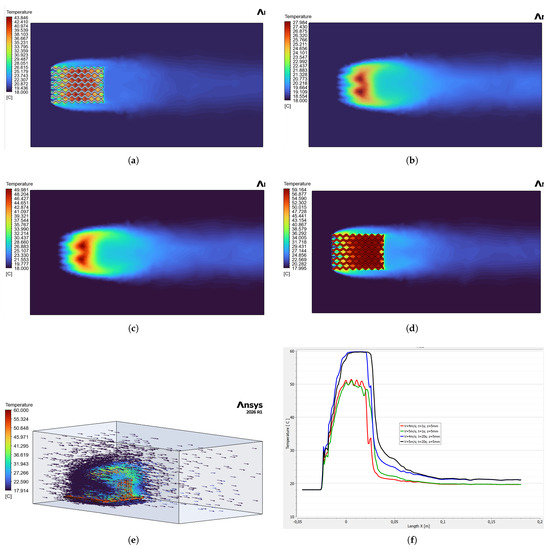
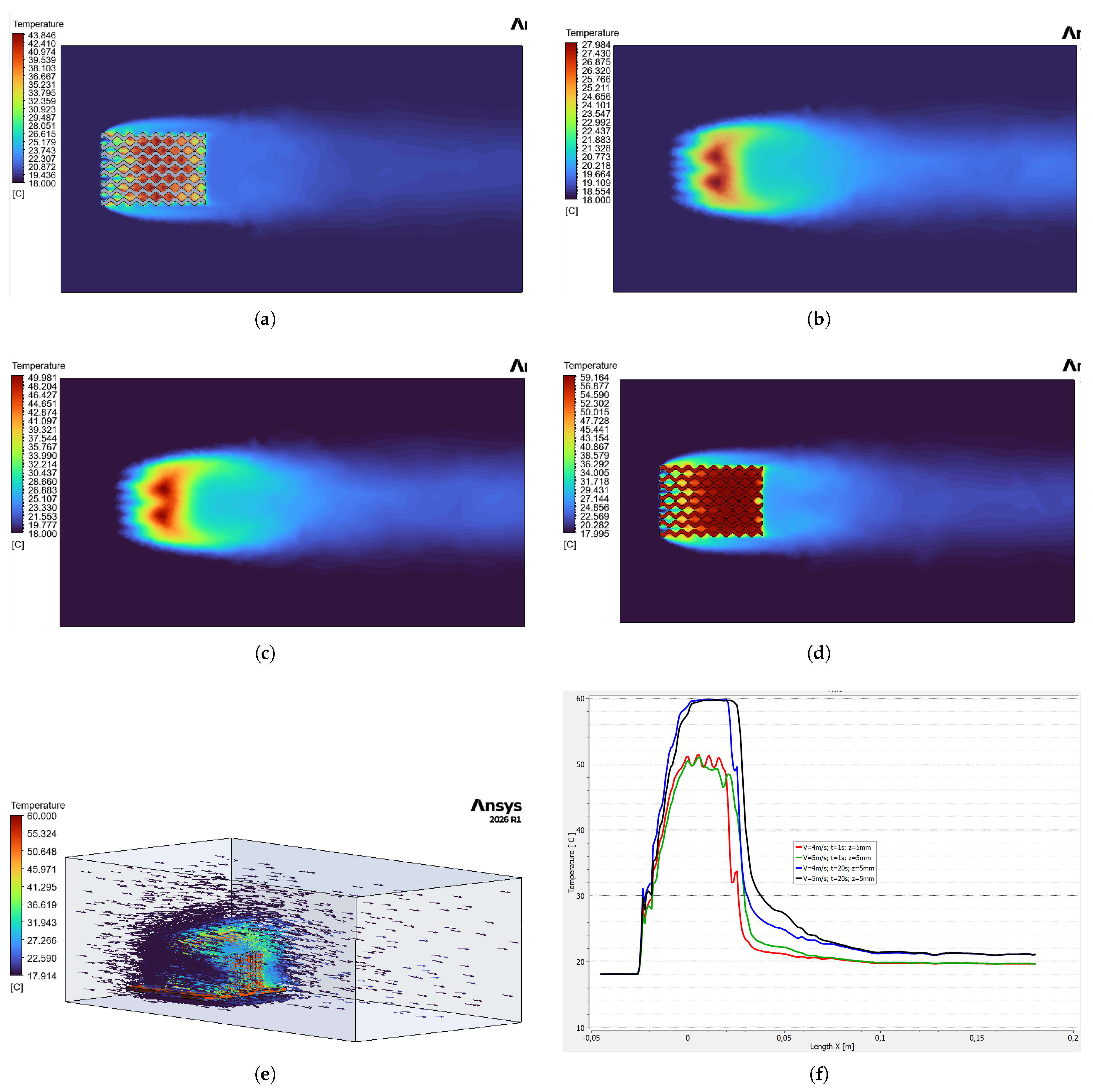
Figure 8 shows the temperature behavior of the sinusoidal heat sink; however, this corresponds to a velocity of 4 m/s, along with a comparison to the incoming airflow at 5 m/s.

Figure 8. Heat sink with sinusoidal fins, velocity of 4 m/s: (a) Temperature contour at 1 s, z = 10 mm. (b) Temperature contour at 1 s, z = 30 mm. (c) Temperature contour at 10 s, z = 30 mm. (d) Temperature contour at 10 s, z = 10 mm. (e) Temperature vector on the heat sink. (f) Temperature comparison at the same height (Z = 5 mm) for durations of 1 s and 20 s and speeds of 4 m/s and 5 m/s.

Since the heat sink is a three-dimensional device, its temperature will vary depending on its height and the duration of exposure to the forced convective environment. Figure 8a shows the temperature contour at an airflow velocity of 4 m/s, at a time of 1 s, and at a height of 10 mm from the base of the heat sink, with a maximum temperature of 43.84 °C, while at the same height after 10 s it is 59.16 °C; this is shown in Figure 8d.

When moving along the z-axis to a distance of 30 mm from the base, the air temperature decreases substantially, reaching a maximum of 27.98 °C at a time of 1 s, Figure 8b, achieving a 36% decrease. This is because the measurement point is located away from the heat sink. On the other hand, after 10 s, the temperature reaches 49.98 °C, a reduction of 15.5%, Figure 8c. When comparing these two percentages with their counterparts at a height of 10 mm, although a linear change in temperature is not expected, it can be quantified that as time passes, the temperature will depend on the position.

On the other hand, Figure 8e shows the temperature vectors across the heat sink, revealing how the temperature is distributed throughout the structure. It can be seen that these vectors are nearly zero near the outer boundaries of the air, while as one approaches the center of the heat sink, the temperature increases until it reaches values of 60 °C near the base of the heat sink. However, it is important to visualize the temperature behavior within the heat sink and the surrounding air in order to quantify how much this variable increases or decreases throughout the system.

Figure 8f illustrates the temperature change for four specific cases at speeds of 4 m/s and 5 m/s, the latter being a significant velocity since it is the highest velocity present in the heat sink, and for two analysis time intervals: 1 s and 20 s. It is worth noting that at a velocity of 5 m/s, the air temperature extends over a greater distance along the x-axis. Regarding temperature, at the 20-s time point, the temperature is very close to 60 °C, whereas at 1 s, these temperatures are around 50 °C. Once the air has left the heat sink and we are at the tail end of the dissipated air, at 1 s intervals the temperature averages 20 °C, while at 20 s intervals it is close to 22 °C. From this, we can infer that as time passes, heat dissipation increases, although it stabilizes after 15 s.

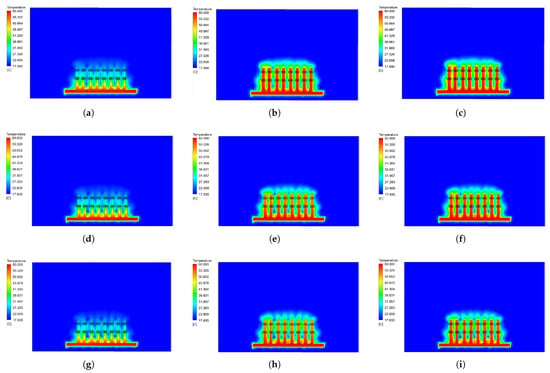
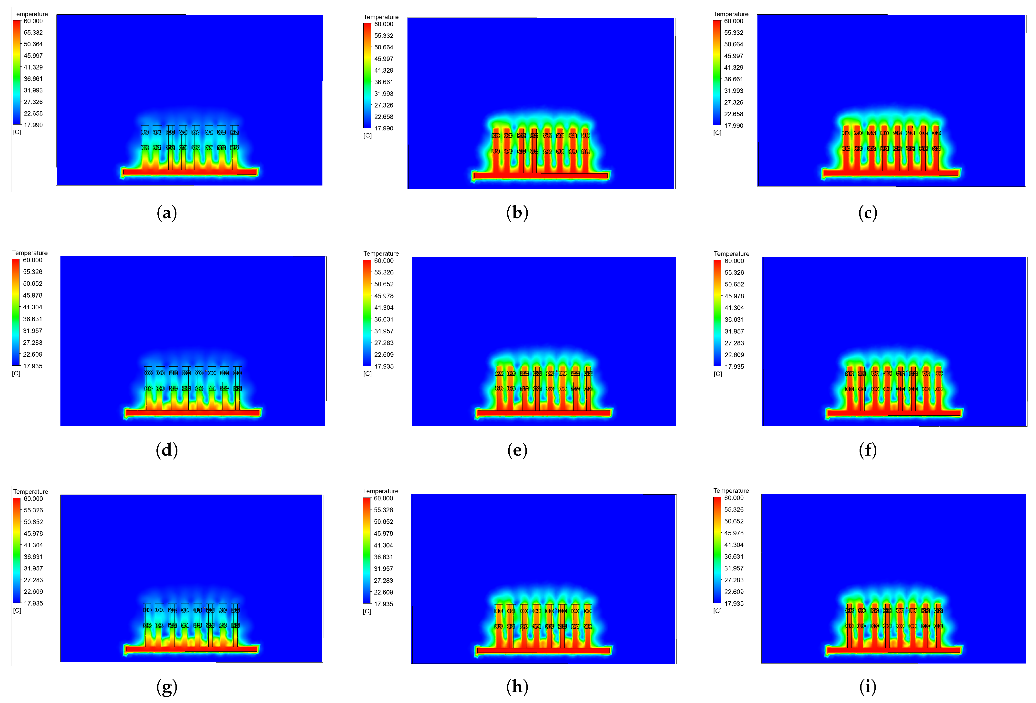
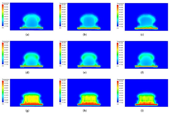
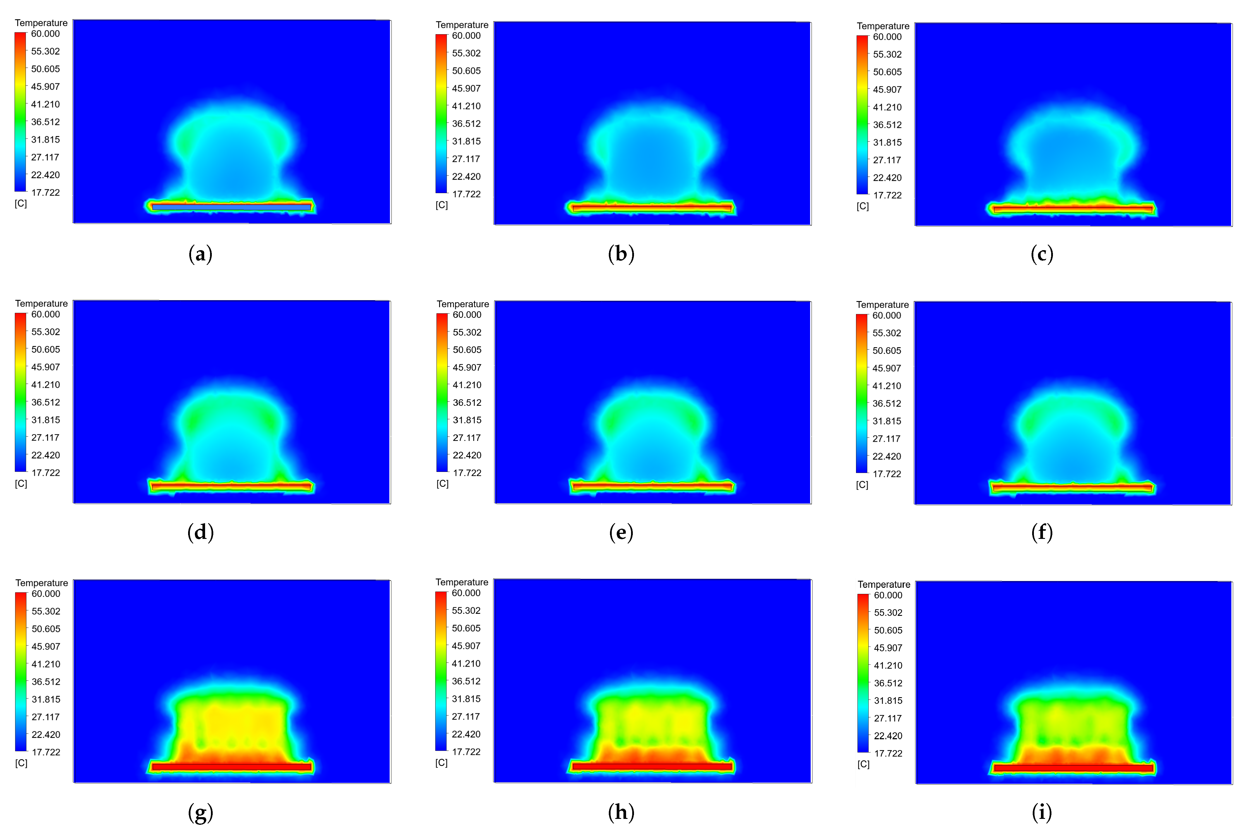
Figure 9 shows how heat dissipates across the three different heat sinks under three different conditions of speed and time. It is important to note that the graphs shown in this figure are temperature contours at the center of the device.

Figure 9. Temperature contours for the heat sink with separate sinusoidal fins, Case C: (a) V = 3 m/s; t = 1 s. (b) V = 3 m/s; t = 5 s. (c) V = 3 m/s; t = 20 s. (d) V = 4 m/s; t = 1 s. (e) V = 4 m/s; t = 5 s. (f) V = 4 m/s; t = 20 s. (g) V = 5 m/s; t = 1 s. (h) V = 5 m/s; t = 5 s. (i) V = 5 m/s; t = 20 s.

The rows represent the velocity in the heat sink with spaced sinusoidal fins: the first row shows a velocity of 3 m/s, the second row a velocity of 4 m/s, and the third row a velocity of 5 m/s. On the other hand, the columns represent the analysis times: the left column shows the time at 1 s, the center column at 5 s, and the right column at 20 s. The analysis at 10 s has been omitted from the figures, as there is not much variation between 10 and 20 s.

Figure 9a,d,g show the heat dissipation for three analysis speeds over a 1 s period; it is clear that heat dissipation is greater at higher speeds. The temperature values at the center of the device are 25.58 °C, 25.15 °C, and 24.87 °C for speeds of 3 m/s, 4 m/s, and 5 m/s, respectively. There is a change of 0.71 °C, which is small; however, if the analysis is performed closer to the base of the heat sink, at a distance of 5 mm, the temperatures 40.94 °C, 47.14 °C, and 48.43 °C for the same speeds described above. It can be seen that there is a temperature change of 7.49 °C, from which it can be inferred that the higher the airflow velocity, the faster the temperature dissipates.

On the other hand, Figure 9b,e,h show the temperature contours at 5 s; these figures provide a clearer view of the heat dissipation from the device. This indicates that significant heat dissipation is achieved after a short time. The temperatures in this case are 36.42 °C, 34.34 °C, and 32.89 °C for the analysis speeds, respectively. Regarding the 1 s time interval, there are variations in each case: 29.76%, 26.03%, and 24.38% increases in temperature after 5 s. Meanwhile, if the height is reduced to 5 mm, the temperatures are 42.82 °C, 49.67 °C, and 51.36 °C; in this case, the maximum temperature variation is 5.7% when the airflow velocity is 5 m/s.

Similarly, Figure 9c,f,i show the temperature contours at 20 s. Visually, there do not appear to be any significant changes between 5 s and 20 s; however, there are noticeable differences when compared to 1 s. Here, the temperatures are 37.91 °C, 35.54 °C, and 33.90 °C, corresponding to the previously mentioned velocities, respectively. The percentage changes in temperature are low, even though the time interval between analyses is 15 s. The percentages are 3.9%, 3.37%, and 2.92% for the speeds of 3 m/s, 4 m/s, and 5 m/s, respectively. This suggests that the greatest temperature change occurs in the first 5 s. When analyzing the temperature at a height of 5 mm, the minimum and maximum temperatures reached in the air surrounding the heat sink are 40.36 °C and 51.71 °C for a time of 20 s and air velocities of 3 m/s and 5 m/s, respectively. This indicates that at higher velocities, the air temperature increases at the same location and over the same time period.

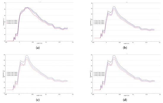
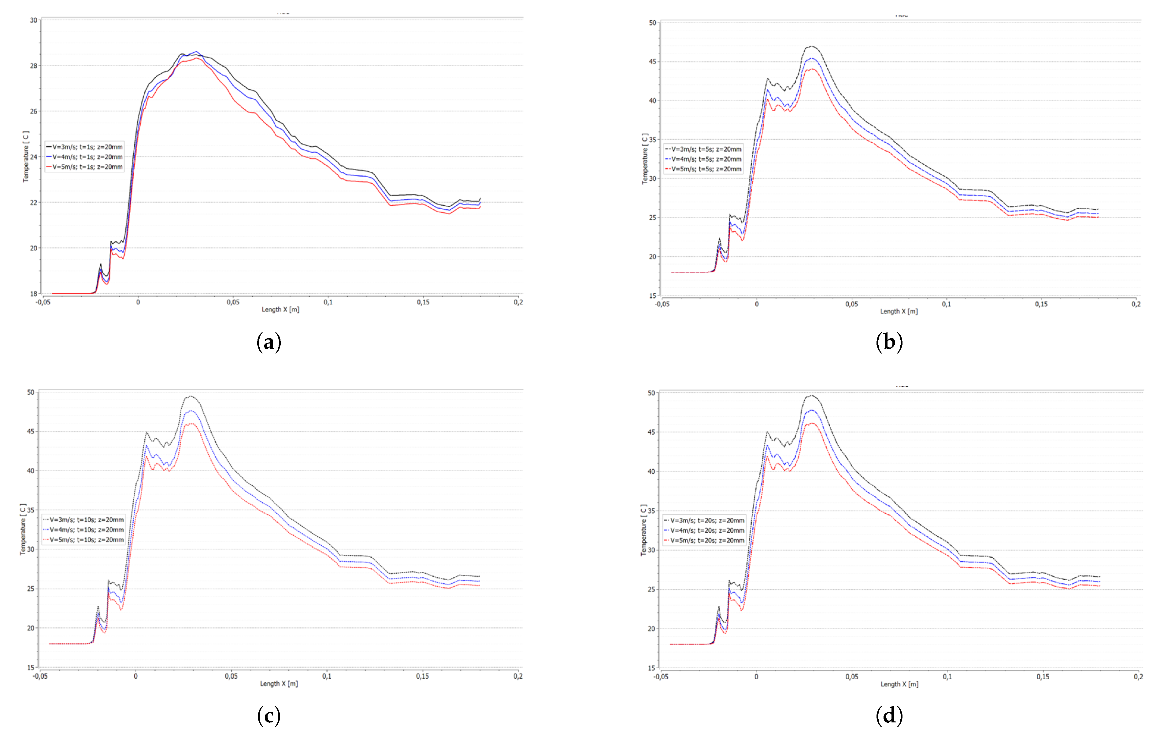
Figure 10 illustrates how the temperature changes from the point where the surrounding air first comes into contact with the heat sink to the end of the heat sink. The analysis is conducted at four different time points, for the three flow rates described for each case, and at a height of 20 mm from the base of the heat sink.

Figure 10. Temperature distribution in the air around the heat sink: (a) t = 1 s. (b) t = 5 s. (c) t = 10 s. (d) t = 20 s.

It is important to note that the temperature refers to that of the air, not the heat sink. Figure 10a shows a temperature increase exceeding 28 °C; however, at a velocity of 3 m/s, the temperature is higher and takes longer to drop compared to a velocity of 5 m/s. Once outside the heat sink, the air temperature begins to drop, averaging 22 °C.

On the other hand, Figure 10b shows that at a simulation time of 5 s, the air temperature reaches 47 °C and 44 °C for wind speeds of 3 m/s and 5 m/s, respectively. There is a difference of 3 °C, once again confirming that air velocity is the most important variable in heat dissipation. However, the average air temperature after heat dissipation is 26 °C, an increase of 4 °C compared to the 1 s time step. This makes it clear that the heated air must be evacuated from the electronic system as soon as possible to prevent overheating.

Finally, Figure 10c,d show the air temperatures at 10 s and 20 s. These figures reveal a slight increase in temperature compared to the 5 s mark, thus confirming that the greatest temperature rise occurs during the first 5 s; however, as heat dissipation continues in the device, temperatures remain constant at values above 20 s.

Figure 11 shows a temperature contour analysis for the three cases at a velocity of 3 m/s. It also illustrates how the temperature changes in the air across three different planes and the benefits of the analysis.

Figure 11. Temperature contours and distribution in the three case studies, at 3 m/s: (a) Case A, t = 5 s. (b) Case B, t = 5 s. (c) Case C, t = 5 s. (d) All cases, x = 30 mm. (e) All cases, x = 50 mm. (f) All cases, x = 100 mm. (g) Temperature distribution, Case C, at the level of the upper holes and on the outermost fin. (h) Velocity profile, Case C, at the level of the upper holes and on the outermost fin.

The temperature contours in the first three sub-figures represent the temperature distribution for the heat sinks with sinusoidal fins, sinusoidal fins with holes, and sinusoidal fins with wider spacing and perforations, respectively.

Figure 11a shows how heat is dissipated into the surrounding air at a velocity of 3 m/s; however, it is clear that there is a concentration of temperature at the base of the heat sink, which begins to rise up the fins. The highest temperature reached is 54 °C at the center of the heat sink at a height of 25 mm; nevertheless, as one moves down toward the base (z = 5 mm), the temperature rises to 58.4 °C. In the area surrounding the heat sink, at a distance of 1 mm, the air temperature drops to an average of 32.5 °C; at greater distances, more drastic changes are observed.

Similarly, Figure 11b shows the temperature distribution for Case B, which features sinusoidal fins with holes at the top of the fin profile. It can be seen that the dissipated air has a higher temperature and that the fins heat up more, suggesting that heat dissipation is improved by adding perforations. The maximum temperature reached in the heat sink, at the same point in the analysis as in Case A, is 55.15 °C, representing an increase of 1.15 °C. On the other hand, near the base (z = 5 mm), the temperature is 58.28 °C. Here, the temperature of the surrounding air decreases very little, suggesting that near the base, where there are no perforations, heat dissipation does not improve. In the surrounding area, the temperature is now 31.75 °C, slightly lower than in Case A; however, it is evident that the heat is dissipating parallel to the air inlet, along the x-axis.

In the same way, Figure 11c shows the temperature distribution for a heat sink with sinusoidal fins that have holes; however, the fins are spaced further apart (Case C). It is easy to see that there are no significant temperature peaks in the center of the heat sink. The temperature barely reaches 44.4 °C; with this modification, a reduction of more than 10 °C has been achieved compared to Cases A and B. In contrast, the temperature at the center of the heat sink is 36.4 °C; here, a very significant change is noticeable in that the surrounding air is no longer as hot as in the previous cases. What is also noticeable is that the hot air fills almost the entire control volume; in other words, the heat flows out of the heat sink.

The other three figures show how the temperature varies in three different scenarios as a function of the x-axis. The three analysis cases are compared at three different distances from the heat sink.

Figure 11d shows the temperature change as air flows through the heat sink; the specific points of analysis are: x = 30 mm, y = 0 mm, z = 20 mm. The analysis is performed along the entire length of the y-axis. There are two different control times: 1 s and 5 s. Once again, the three cases were studied. It appears that for Case A, the heat dissipation temperature is not as high in the two evaluated time intervals, reaching 24 °C at 1 s and 33 °C at 5 s as maximum temperature peaks. However, upon examining Case B, a slight increase in temperature is observed at 1 s, reaching 25 °C, and at 5 s, it is 35 °C. This trend continues when analyzing Case C, where the maximum temperatures obtained are 29 °C and 46 °C for 1 s and 5 s, respectively.

Figure 11e shows a shift in the analysis point; the distance along the x-axis has been changed to 50 mm. The temperatures at 1 s show almost no significant changes. However, upon observation at the 5 s time point, significant changes in temperature are noted: for Case A, the maximum temperature reached is 27.5 °C; for Case B, it is 29 °C; and for Case C, it is 40.5 °C. These represent variations of 20%, 20.6%, and 13.5% for Cases A, B, and C, respectively.

Figure 11f shows the temperature analysis as the analysis point is moved; now, the x-axis is a distance of 100 mm. This shows that Case C dissipates heat more effectively at any time, as it exhibits significant temperature values in the surrounding air, reaching a maximum of 30 °C at 5 s, while the other cases barely reach 24 °C at that same time.

On the other hand, Figure 11g provides a closer look at what happens with the temperature in the area of the upper holes in the fins; here, it is clearly visible how cold air enters through the holes and cools the heat sink more effectively. Similarly, Figure 11h shows the velocity distribution through the spaces between the fins and the upper holes, revealing that the flow passes through all of them—initially at a very high speed and then gradually decaying. However, the flow performance across the entire heat sink is notable.

Figure 12 compares the three case studies, the three different types of heat sinks, using the three analysis speeds. However, it should be noted that the analyses are displayed at a time of 5 s, as that is the point at which the inflection point in heat dissipation occurs.

Figure 12. Comparison of temperature contours at the three analysis speeds at 5 s and at a distance of x = 30 mm: (a) Case A, V = 3 m/s. (b) Case A, V = 4 m/s. (c) Case A, V = 5 m/s. (d) Case B, V = 3 m/s. (e) Case B, V = 4 m/s. (f) Case B, V = 5 m/s. (g) Case C, V = 3 m/s. (h) Case C, V = 4 m/s. (i) Case C, V = 5 m/s.

Figure 12a, Figure 12b and Figure 12c show the temperature distribution on the heat sink without holes at flow velocities of 3 m/s, 4 m/s, and 5 m/s, respectively. Figure 12a shows that the temperature at the base of the heat sink is not as high at a velocity of 3 m/s, with a value of 28.86 °C, while for the other two velocities, the values are 32.50 °C and 43.03 °C. Showing substantial changes in heat dissipation, there are increases of 11.2% and 32.93% relative to the lowest velocity. On the other hand, Figure 12b shows an increase in temperature around the heat sink, while in the central area, the temperature decreases from 30.16 °C to 25.74 °C. This suggests that air is not circulating freely between the sinusoidal fins. Similarly, Figure 12c, with a velocity of 5 m/s, shows values similar to those in the previous figure. However, a temperature increase is observed in the region near the base, with the temperature rising to 43.03 °C.

Figure 12d–f show the simulations for fin type B, which features sinusoidal fins with perforations at the top of the fin; the three speeds studied are included. As with the simulations for Case A, a cold temperature bubble is observed in the central area of the heat sink. However, the temperature near the base now remains similar for the analyzed velocities: 29.38 °C, 29.88 °C, and 28.50 °C, respectively. The variation in Case B is less than 1 °C at that point of analysis, from which it can be deduced that the application of perforations results in a more uniform heat dissipation temperature. However, at the height where the holes are located, the temperature of the dissipated air is higher, reaching 34.04 °C, which is higher than in Case A.

Finally, the row of Figure 12g–i shows the temperature contours for Case C, where significant changes in the dissipated heat can be observed; these changes are due to the fact that, in this case, the fins are spaced apart. Now, the temperature at the base for wind speeds of 3 m/s, 4 m/s, and 5 m/s is as follows: 54.64 °C, 56.15 °C, and 54.24 °C. in this case, the three temperatures remain similar; however, when compared to Cases A and B, percentage increases of 47.18% and 46.22% are observed for the 3 m/s velocity. Meanwhile, for the 4 m/s velocity, the changes are 42.11% and 48.88%. Similarly, for the maximum velocity of 5 m/s, the variations are 20.66% and 47.45 °C. This indicates that there is an improvement of approximately 47% in heat dissipation when using sinus-shaped fins with holes. Specifically, Figure 12i shows that the temperature rises with fin height. Therefore, in this study, higher speeds and greater fin spacing improve heat dissipation.

4. Conclusions

The present numerical study investigated the transient thermal performance of three sinusoidal-fin heat sink configurations under forced convection: solid fins (Case A), fins with circular perforations (Case B), and fins with combined perforations and variable inter-fin spacing (Case C). Using ANSYS Fluent 2025 R2 with a validated mesh, the following conclusions are drawn:

The transient analysis reveals that, in all cases, more than 85% of the total temperature increase occurs during the first 5 s. This occurs at a height of 5 mm along the z-axis, measured from the base; 15 mm along the x-axis, after exiting the heat sink; and 0 mm along the y-axis. This finding implies that improvement strategies should focus on optimizing the thermal response under transient conditions rather than under steady-state conditions.

In the unperforated heat sink (Case A), the rate of temperature increase in the air between t = 10 s and t = 14 s was just 0.31 °C, representing a slope of 0.0775 °C/s. This behavior confirms that the system reaches a quasi-steady state in less than 14 s, a relevant finding for applications with intermittent thermal loads.

At t = 1 s and at a height of 5 mm above the base, the air temperature rose from 40.94 °C to 48.43 °C as the velocity increased from 3 m/s to 5 m/s. This 18.3% increase demonstrates that, in the initial moments, forced convection strongly modulates the temperature gradient near the active surface.

The inclusion of perforations reduced the solid transfer area by 5.94%, but the base temperature in Case B remained stable despite changes in velocity. This result suggests that the increase in turbulence quantitatively compensates for the loss of conductive surface area, at least within the evaluated velocity range.

The average skewness remained between 0.2357 and 0.2423 in all cases, values well below the threshold of 0.25 considered excellent in the CFD literature. This provides statistical support for the convergence and reproducibility of the simulations.

The combined perforation and variable-spacing configuration (Case C) achieves thermal performance comparable to the other cases while introducing design flexibility for non-uniform heat loads. The alternating spacing (2 mm and 4.5 mm) creates localized flow acceleration and deceleration zones, which can be strategically tailored to match the heat flux distribution of specific electronic components. This finding provides a practical design guideline: for applications with uneven heat generation, variable spacing fin arrays can be customized to allocate cooling capacity precisely where it is most needed, improving overall system reliability and reducing the risk of hotspots.

From a thermal-fluid dynamics perspective, the perforations act as passive flow control devices that generate localized jet-like effects and vortex shedding downstream of each hole. These flow disturbances enhance mixing between the near-wall fluid and the core flow, effectively disrupting the thermal boundary layer and promoting convective heat transfer. The net result is that the turbulence-induced enhancement in the convective heat transfer coefficient compensates for and in some cases surpasses the effect of the loss of conductive surface area.

References

- Sallar, H.; Irfan, M.; Khan, M.M.; Shahzad, M.W. Hydro-thermal performance of an I-shaped pin fin microchannel heat sink with variable pin fin height, thickness and orientation. Int. Commun. Heat Mass Transf. 2025, 160, 108256. [Google Scholar] [CrossRef] [Scilit]
- Fattahi, R.; Saidi, M. Numerical investigation of curved shape fins height effect on heat transfer and flow characteristics in open microchannel heat sink. Int. J. Therm. Sci. 2023, 185, 108060. [Google Scholar] [CrossRef] [Scilit]
- Ribatski, G.; Cabezas-Gómez, L.; Navarro, H.; Saíz-Jabardo, J. The advantages of evaporation in micro-scale channels to cool microeletronic devices. Therm. Eng. 2007, 6, 34–39. [Google Scholar] [CrossRef] [Scilit]
- Zhang, Z.; Wang, X.; Yan, Y. A review of the state-of-the-art in electronic cooling. E-Prime Electr. Eng. Electron. Energy 2021, 1, 100009. [Google Scholar] [CrossRef] [Scilit]
- Liang, G.; Mudawar, I. Review of spray cooling–Part 1: Single-phase and nucleate boiling regimes, and critical heat flux. Int. J. Heat Mass Transf. 2017, 115, 1174–1205. [Google Scholar] [CrossRef] [Scilit]
- Sultan, H.S.; Saleem, K.B.; Alshammari, B.M.; Turki, M.; Aydi, A.; Kolsi, L. Numerical investigation of natural convection from a horizontal heat sink with an array of rectangular fins. Case Stud. Therm. Eng. 2024, 61, 104877. [Google Scholar] [CrossRef] [Scilit]
- Meng, X.; Zhu, J.; Wei, X.; Yan, Y. Natural convection heat transfer of a straight-fin heat sink. Int. J. Heat Mass Transf. 2018, 123, 561–568. [Google Scholar] [CrossRef] [Scilit]
- Tepe, A.Ü.; Yetişken, Y.; Uysal, Ü.; Arslan, K. Experimental and numerical investigation of jet impingement cooling using extended jet holes. Int. J. Heat Mass Transf. 2020, 158, 119945. [Google Scholar] [CrossRef] [Scilit]
- Alihosseini, Y.; Targhi, M.Z.; Heyhat, M.M.; Ghorbani, N. Effect of a micro heat sink geometric design on thermo-hydraulic performance: A review. Appl. Therm. Eng. 2020, 170, 114974. [Google Scholar] [CrossRef] [Scilit]
- Arshad, A.; Jabbal, M.; Yan, Y. Preparation and characteristics evaluation of mono and hybrid nano-enhanced phase change materials (NePCMs) for thermal management of microelectronics. Energy Convers. Manag. 2020, 205, 112444. [Google Scholar] [CrossRef] [Scilit]
- İzci, T.; Koz, M.; Koşar, A. The effect of micro pin-fin shape on thermal and hydraulic performance of micro pin-fin heat sinks. Heat Transf. Eng. 2015, 36, 1447–1457. [Google Scholar] [CrossRef] [Scilit]
- Yaseen, S.J.; Radhi, Z.K.; Natoosh, R.L.; Al-Sabur, R.; Homod, R.Z.; Mohammed, H.I. A computational search for the optimal microelectronic heat sink using ANSYS Icepak. Int. J. Thermofluids 2024, 23, 100759. [Google Scholar] [CrossRef] [Scilit]
- Tripathy, T.L.; Dash, S.K. Numerical modeling of natural convection heat transfer from radial branching heat sinks for LED cooling applications. Appl. Therm. Eng. 2024, 242, 122446. [Google Scholar] [CrossRef] [Scilit]
- Ray, R.; Mohanty, A.; Patro, P.; Senapati, S.K. Performance improvement of a heat sink with triangular slotted and interrupted fins: A computational study. Appl. Therm. Eng. 2023, 230, 120783. [Google Scholar] [CrossRef] [Scilit]
- Abdulsahib, A.D.; Alkhafaji, D.; Albayati, I.M. Improving the natural convection of the heat sink inside an enclosure by fin perforation for electronic applications. Heat Transf. 2025, 54, 389–419. [Google Scholar] [CrossRef] [Scilit]
- Raza, S.S.; Bhushan, R. A Comprehensive Review on Computational Fluid Dynamics Analysis and Optimization of Open Micro-Channel Heat Sinks with Pin Fins. Int. J. Res. Appl. Sci. Eng. Technol. 2024, 12, 884–893. [Google Scholar] [CrossRef] [Scilit]
- Huang, C.H.; Xu, E.H. Optimization of natural convection heat sinks with inverted trapezoidal fins and elliptical perforations. Int. J. Therm. Sci. 2026, 222, 110581. [Google Scholar] [CrossRef] [Scilit]
- Taha, M.S.; Ates, A.; Canli, E.; Altun, A.H. Circular perforations on vertically sinusoidal wave form plate fin heat sinks for laminar natural convection heat dissipation. Int. J. Therm. Sci. 2025, 208, 109470. [Google Scholar] [CrossRef] [Scilit]
- Dastbelaraki, A.; Yaghoubi, M.; Tavakol, M.; Rahmatmand, A. Numerical analysis of convection heat transfer from an array of perforated fins using the Reynolds averaged Navier–Stokes equations and large-eddy simulation method. Appl. Math. Model. 2018, 63, 660–687. [Google Scholar]
- Ge, Y.; Yin, W.; Lin, Y.; He, K.; He, Q.; Huang, S.M. Multi-objective optimization of a non-uniform sinusoidal mini-channel heat sink by coupling genetic algorithm and CFD model. Appl. Therm. Eng. 2024, 257, 124198. [Google Scholar] [CrossRef] [Scilit]
- Al-Luhaibi, R.A.; Nazzal, I.T. Investigation of Heat Sinks with Different Perforation Patterns. Int. J. Heat Technol. 2023, 41, 1195–1204. [Google Scholar] [CrossRef] [Scilit]
- Çengel, Y.A.; Ghajar, A.J. Heat and Mass Transfer: Fundamentals & Applications; McGraw Hill LLC: Columbus, OH, USA, 2025. [Google Scholar]
- Silva, J.A.d.; Silva, L.P.d.; Campos, J.C.C.; Siqueira, A.M.d.O.; Gurgel, A.; Gómez, L.C. Dynamic mesh analysis by numerical simulation of internal combustion engines. REM-Int. Eng. J. 2024, 77, 27–37. [Google Scholar] [CrossRef] [Scilit]
- Fluent, A. Ansys fluent theory guide. 2026.
- Garrido, P.L.; Hurtado, P.I.; Nadrowski, B. Simple one-dimensional model of heat conduction which obeys Fourier’s law. Phys. Rev. Lett. 2001, 86, 5486. [Google Scholar] [CrossRef] [Scilit] [PubMed]
- Soto, R.; Mareschal, M.; Risso, D. Departure from Fourier’s law for fluidized granular media. Phys. Rev. Lett. 1999, 83, 5003–5006. [Google Scholar] [CrossRef] [Scilit]
- Madhavadas, V.; Das, D.; Mohta, K.A.; Senthur Prabu, S. Comparative analysis on heat transfer of various fin profile using solid works: A systematic review. In Proceedings of the IOP Conference Series: Earth and Environmental Science; IOP Publishing: Bristol, UK, 2021; Volume 850, p. 012029. [Google Scholar]
- Incropera, F.P.; DeWitt, D.P.; Bergman, T.L.; Lavine, A.S.; Incroper, F.P.; Dewit, D.P. Fundamentals of Heat and Mass Transfer; Wiley New York: New York, NY, USA, 2011; Volume 6. [Google Scholar]
- Ma, H.; Cai, N.; Cai, L.; Si, F. Effects of the forced convection induced by assistant fans on the thermal performance of an indirect dry cooling system. Case Stud. Therm. Eng. 2022, 35, 102141. [Google Scholar] [CrossRef] [Scilit]
- Kirchhofer, M.; Krieger, M.; Hofer, D. Experimental and numerical investigations of forced convection impingement heat transfer on plate-fin heat sinks using three different electronic cooling fans. Appl. Therm. Eng. 2025, 258, 124665. [Google Scholar] [CrossRef] [Scilit]
Disclaimer/Publisher’s Note: The statements, opinions and data contained in all publications are solely those of the individual author(s) and contributor(s) and not of MDPI and/or the editor(s). MDPI and/or the editor(s) disclaim responsibility for any injury to people or property resulting from any ideas, methods, instructions or products referred to in the content. |
© 2026 by the authors. Licensee MDPI, Basel, Switzerland. This article is an open access article distributed under the terms and conditions of the Creative Commons Attribution (CC BY) license.