Ultra-Short-Term Photovoltaic Power Forecasting Based on an Improved Spatio-Temporal Joint Attention Mechanism

Abstract

This paper proposes a novel forecasting model termed U-Client, which integrates parallel cross-temporal and cross-variable attention branches with an adaptive gated fusion mechanism for ultra-short-term photovoltaic (PV) power forecasting. First, meteorological features are screened using the Pearson correlation coefficient to reduce input dimensionality. Second, parallel cross-temporal and cross-variable attention branches are designed to extract long-range temporal trends and nonlinear interaction features among meteorological variables, respectively. Third, a gating mechanism is introduced to adaptively fuse the two types of features based on input conditions. Finally, a linear module is combined to generate the final forecasting results. Experiments based on measured datasets from a photovoltaic station in Ningxia, China, demonstrate that the proposed U-Client model outperforms classical models such as Long Short-Term Memory (LSTM) and Informer across all evaluation metrics for 1–4 step forecasting tasks. Ablation studies and statistical significance tests further verify the effectiveness of each component. The proposed model provides reliable support for ultra-short-term power dispatching in new-type power systems.

1. Introduction

Global demand for renewable energy has led to a significant increase in the proportion of renewable energy integrated into the power grid [1], with photovoltaic (PV) power being a particularly notable example. PV power is a key source for meeting the world’s growing energy needs. It is abundant, clean, and environmentally friendly, as well as low-cost and highly efficient [2]. However, solar energy is highly volatile and strongly affected by weather conditions, leading to instability in grid-connected PV power generation [3]. Therefore, accurate forecasting of the nonlinear and uncertain characteristics of PV power output is essential for ensuring the reliable dispatch and operation of power systems [4].

With the continuous development of artificial intelligence algorithms, deep learning models have been widely applied to time-series forecasting tasks. In PV power forecasting, such models can learn the mapping relationship between meteorological factors and PV power output from historical data, thereby accurately forecasting future PV generation. Among them, Graph Convolutional Networks (GCNs) [5,6,7], Long Short-Term Memory (LSTM) networks [8,9], and Light Gradient Boosting Machine (LightGBM) models [10,11] have attracted considerable attention. Reference [12] proposed a hybrid model integrating an LSTM network with a multi-head attention mechanism for short-term PV power forecasting, in which the attention mechanism adaptively weights informative time steps. Reference [13] introduced a LightGBM-based short-term PV generation forecasting model using multi-feature fusion. Reference [14] developed an ensemble neural network forecasting method and improved forecasting accuracy by optimizing model parameters using a heuristic optimization algorithm.

However, when addressing PV power forecasting tasks characterized by strong fluctuations and complex temporal dependencies [15,16], traditional deep learning models still exhibit certain limitations in modeling capability [17]. To overcome these limitations, the Transformer model, originally developed for natural language processing tasks, has gradually been introduced into time-series forecasting applications. Transformer replaces recurrent structures with self-attention, enabling parallel computation and effective modeling of long-range dependencies [18]. Subsequently, various Transformer-based models such as Informer [19] and Autoformer [20] have been proposed for time-series forecasting tasks.

In addition, spatio-temporal deep learning approaches have shown strong potential for renewable energy forecasting and downstream grid dispatch. For instance, graph-based spatio-temporal neural networks have been applied to multi-site PV forecasting [21], and graph-attention-based architectures have been used for regional short-term PV power forecasting by exploiting spatial correlations among distributed PV stations [22].

However, most existing Transformer variants rely on a single attention mechanism, which has limited capabilities for jointly modeling temporal and variable dimensions; consequently, they do not adequately capture the interrelationships between different time scales and variables [23]. In PV power forecasting, PV output is influenced not only by the temporal evolution of historical power sequences but also by complex interactions among meteorological factors. To effectively model these two types of dependencies simultaneously, this paper develops an improved forecasting model based on the Client architecture by introducing a gated fusion mechanism integrating cross-temporal attention and cross-variable attention. Furthermore, a learnable gating unit adaptively fuses the two types of information, enabling the model to dynamically adjust its focus according to different forecasting scenarios, thereby achieving more accurate PV power forecasting.

2. Transformer Model

Transformer is a deep learning architecture centered on the attention mechanism. It first achieved remarkable success in natural language processing tasks and has subsequently been widely applied in computer vision and time-series forecasting [24].

When processing sequential data, traditional recurrent neural networks (RNNs) generally transmit information step by step along the temporal dimension [25]. Although this mechanism can capture certain temporal relationships, it often suffers from information loss, difficulty in modeling long-range dependencies, and slow training speed when handling long sequences. In contrast, Transformer introduces the attention mechanism, which directly computes the correlation between any two positions in a sequence without requiring recurrence. This innovation substantially improves the model’s ability to capture long-range dependencies while significantly enhancing parallel computing efficiency.

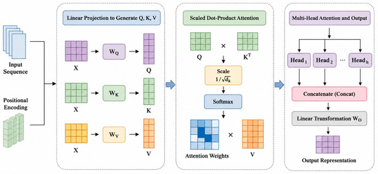
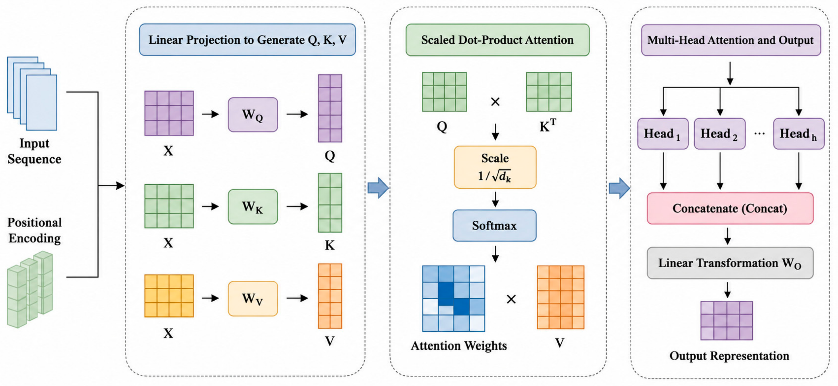
From the perspective of overall architecture, a standard Transformer model generally consists of two core components: the encoder and the decoder [26]. The encoder is responsible for extracting high-level semantic features from the input data, whereas the decoder utilizes these extracted features to generate the final output sequence. In practical engineering applications, researchers often fine-tune the Transformer architecture according to specific task requirements to further improve its ability to capture local features and adapt to dynamic variations. The Transformer model architecture used in this article is shown in Figure 1.

Figure 1. Transformer model architecture.

3. U-Client Model

The Client model (Cross-variable Linear Integrated Enhanced Transformer), proposed by Gao et al. [27] and published in AI Open (2025), is a novel long-term time-series forecasting model. Its primary innovation lies in integrating cross-variable attention into the Transformer module to learn dependency relationships between forecasting target variables and feature factors. Specifically, in photovoltaic (PV) power forecasting tasks, historical PV power sequences and meteorological feature data, including irradiance and temperature, are regarded as different entities.

The attention mechanism assigns larger weights to variables that are more relevant to PV power output. This adaptive weighting mechanism enables the model to prioritize influential factors while suppressing variables with limited forecasting significance. In addition, the model integrates a linear module to capture historical trends in PV power generation and a RevIN module to alleviate distribution shifts in PV sequences. The Reversible Instance Normalization (RevIN) [28] plays a critical role in handling distribution shifts commonly observed in PV power sequences across different seasons and weather patterns. It normalizes input sequences to zero mean and unit variance before model processing, and denormalizes the output after forecasting. This process reduces the influence of distributional variations and improves model robustness. In our ablation experiments, removing the RevIN module leads to a MAPE increase from 13.59% to 15.12% for one-step forecasting, confirming its significant contribution to forecasting accuracy, particularly under non-stationary weather conditions.

This paper proposes a forecasting model termed U-Client, which integrates parallel cross-temporal and cross-variable attention branches with an adaptive gated fusion mechanism for ultra-short-term photovoltaic (PV) power forecasting. First, meteorological features are screened using the Pearson correlation coefficient to reduce input dimensionality. Second, the parallel cross-temporal and cross-variable attention branches extract long-range temporal trends and nonlinear inter-variable interactions, respectively. Third, a gating mechanism adaptively fuses the two feature types. Finally, a linear projection module generates the forecasting results. Experiments on a measured dataset from a PV station in Ningxia, China, and the public DKASC benchmark demonstrate that U-Client achieves lower RMSE, MAE, and MAPE than classical and state-of-the-art baselines across all forecasting horizons, providing reliable support for ultra-short-term power dispatching.

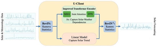
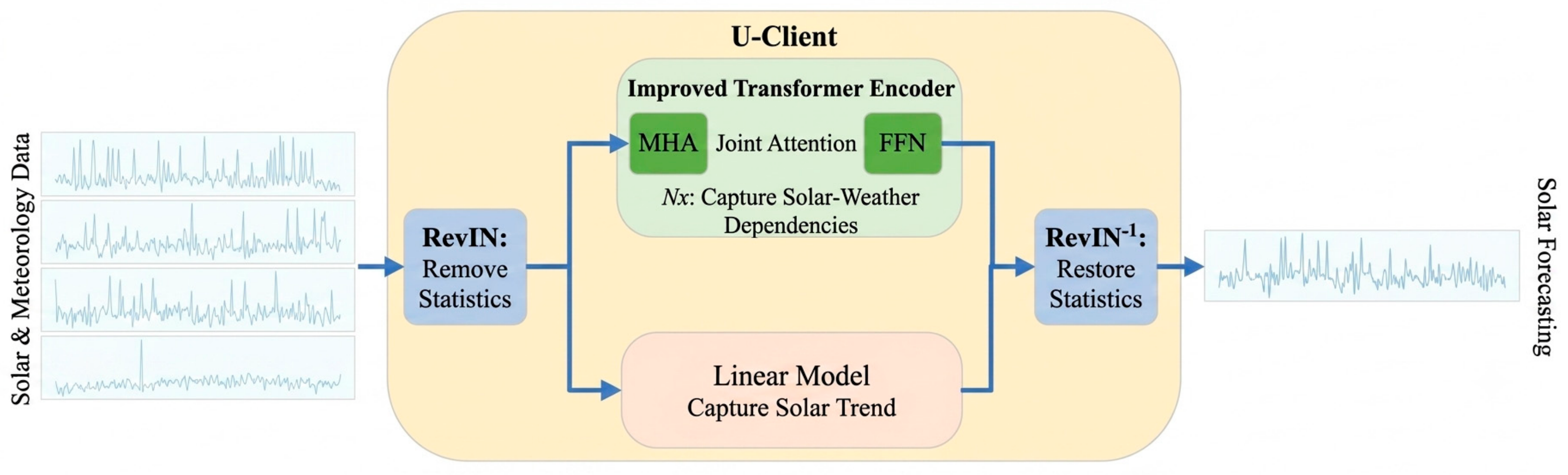
Figure 2 illustrates the overall architecture of the U-Client model. These architectural designs enable the model to more effectively exploit variable dependencies and temporal trends in PV power data. The individual components of the U-Client model are described in detail in the following sections.

Figure 2. U-Client architecture diagram.

Based on the Client architecture, this paper further optimizes the design of multidimensional attention mechanisms. The original model captures dependency relationships between PV power and meteorological variables only along the temporal dimension through the Transformer encoder. Therefore, this study designs parallel cross-temporal and cross-variable attention branches and adaptively fuses information from both dimensions through a gated fusion mechanism, forming a spatio-temporal joint attention mechanism. The mathematical derivation of this process is as follows:

The input sequence is:

$$X\in {ℝ}^{L\times D}$$

(1)

where $L$ denotes the historical time-step length and $D$ represents the number of variables.

3.1. Cross-Temporal Attention Mechanism

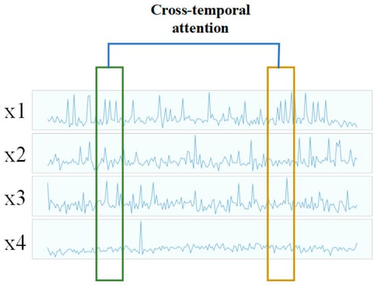
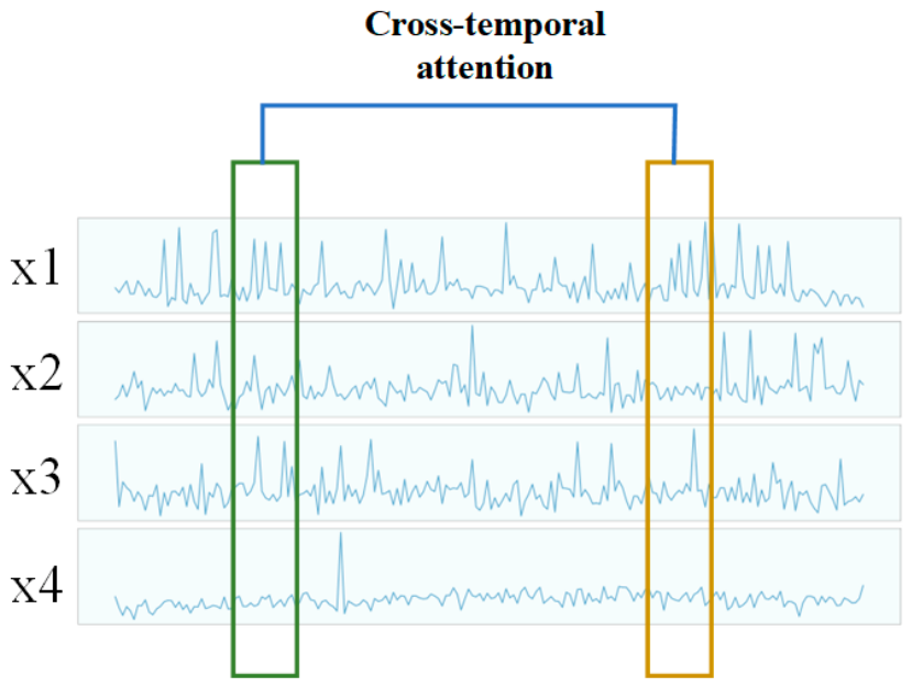
Cross-temporal attention is calculated along the temporal dimension to characterize dependency relationships among different time steps, as shown in Figure 3. The calculation process is expressed as follows:

$$Q_t=X{W}_t^Q,K_t=X{W}_t^K,V_t=X{W}_t^V$$

(2)

$$H_t=Softmax\left({\displaystyle \frac{Q_t{K}_t^T}{\sqrt{d_k}}}\right)V_t$$

(3)

where $W_t^Q,W_t^K,W_t^V$ are learnable parameter matrices, $d_k$ denotes the dimension of the key vector, and $H_t\in {ℝ}^{L\times D}$ represents the temporal attention output. This branch mainly extracts periodicity, trends, and abrupt temporal variations in the PV power sequence.

Figure 3. Cross-temporal attention.

3.2. Cross-Variable Attention Mechanism

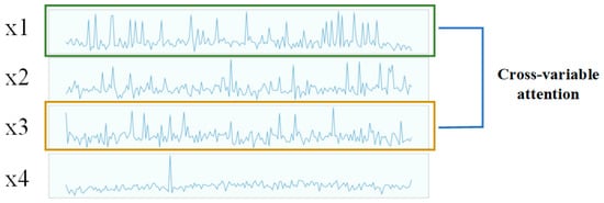
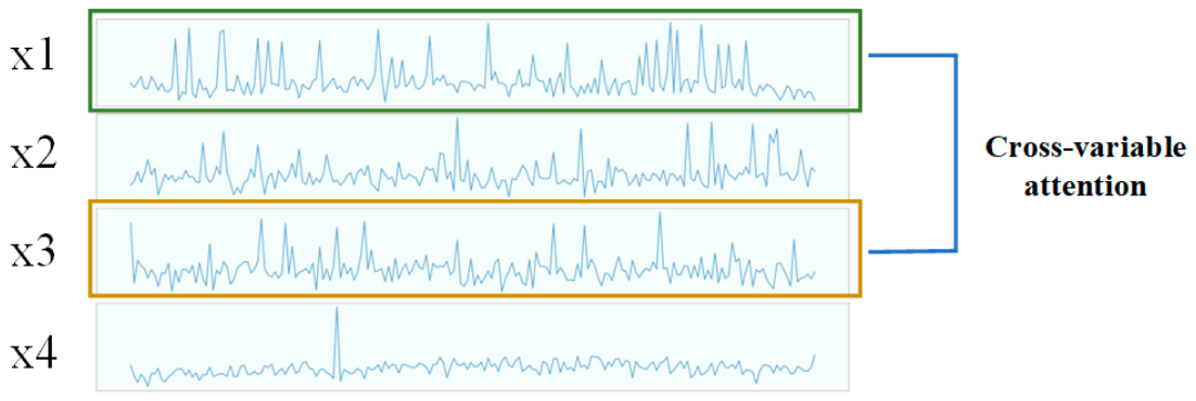
Cross-variable attention models the interactions between PV power and meteorological variables by transposing the input sequence so that variables become attention tokens. This allows us to model the mutual influence between photovoltaic power and meteorological factors in a multivariate framework, as shown in Figure 4.

Figure 4. Cross-variate attention.

Transpose the input into $X^{{\rm T}}\in {ℝ}^{L\times D}$, then compute:

$$Q_{\upsilon }=X^{{\rm T}}{W}_{\upsilon }^Q,K_{\upsilon }=X^{{\rm T}}{W}_{\upsilon }^K,V_{\upsilon }=X^{{\rm T}}{W}_{\upsilon }^V$$

(4)

$$H_{\upsilon }=Softmax\left({\displaystyle \frac{Q_{\upsilon }{K}_{\upsilon }^T}{\sqrt{d_k}}}\right)V_{\upsilon }$$

(5)

where $W_{\upsilon }^Q,W_{\upsilon }^K,W_{\upsilon }^V$ are learnable parameter matrices in the variable dimension, and $H_{\upsilon }\in {ℝ}^{L\times D}$ denotes the variable attention output. To facilitate subsequent fusion with temporal attention features, the output is transposed back to the standard representation:

$${\tilde{H}}_{\upsilon }=H_{\upsilon }^{{\rm T}}\in {ℝ}^{L\times D}$$

(6)

This branch explicitly learns the influence strength and interaction relationships among different meteorological variables in PV power forecasting.

3.3. Adaptive Gated Fusion Mechanism

After obtaining cross-temporal features $H_t$ and cross-variable features ${\tilde{H}}_{\upsilon }$, a gating mechanism is employed for adaptive feature fusion. The gating weights are calculated as follows:

$$\alpha =\sigma \left(H_t{W}_g+b_g\right)$$

(7)

where $\sigma \left(\cdot \right)$ denotes the Sigmoid activation function, $W_g\in {ℝ}^{D\times D}$ and $b_g\in {ℝ}^D$ are learnable parameters, and $\alpha \in {ℝ}^{L\times D}$ represents the gating coefficient.

The fused feature representation is then expressed as:

$$H_{cv}=\alpha \odot H_t+\left(1-\alpha \right)\odot {\tilde{H}}_{\upsilon }$$

(8)

where $\odot$ denotes element-wise multiplication. This fusion strategy enables the model to adaptively adjust the contribution ratios of temporal dependency information and variable dependency information according to different time steps and feature distributions.

The gating mechanism adaptively balances temporal and variable features according to input conditions. Under stable weather conditions, temporal features dominate forecasting performance, whereas variable interactions become more important during rapidly changing weather. The gate coefficient is generated from the temporal representation $H_t$, allowing the model to preserve the dominant diurnal pattern while incorporating meteorological corrections when necessary.

To implement the above mechanism, the encoding modules of both branches consist of two core components in the Transformer encoder: the Multi-Head Attention (MHA) module [29] and the Feed-Forward Network (FFN) module [30]. The MHA module divides the attention calculation into multiple heads, enabling the model to capture diverse dependency patterns from different representation subspaces in parallel. The FFN module further transforms and enhances the extracted features through nonlinear mappings.

In the cross-temporal branch, MHA is mainly used to learn global dependencies among different time steps, while the FFN refines temporal features. In the cross-variable branch, MHA models the interactions between PV power and meteorological variables using transposed inputs, and the FFN further enhances variable representations. Finally, the extracted features from the two branches are fused through the gating unit and passed into the subsequent projection layer to generate forecasting results.

In U-Client, the cross-variable Transformer primarily serves as a feature extractor rather than a sequence generator, and essentially does not model cross-variable temporal dependencies; therefore, a decoder is no longer necessary. The projection process is described as follows:

$$F_{trans}=\mathrm{Pr}oj\left(X_{enc}\right).Permute\left(1,0\right)$$

(9)

where $X_{enc}$ represents the output of the encoder module and $F_{trans}$ represents the cross-variable transformer forecasting. $Permute\left(1,0\right)$ indicates a swap between the first and second dimensions, which effectively flips the output of the projection layer. After inversion, the output shape aligns with the input figure. The forecastings generated by the cross-variable transformer typically capture the fine details of the PV power output.

4. PV Power Forecasting Procedure

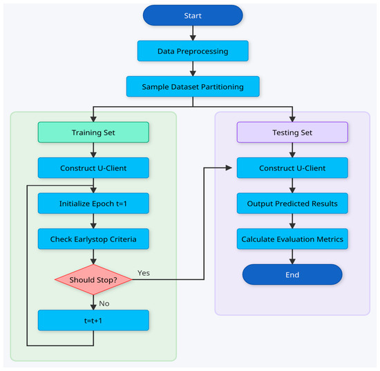
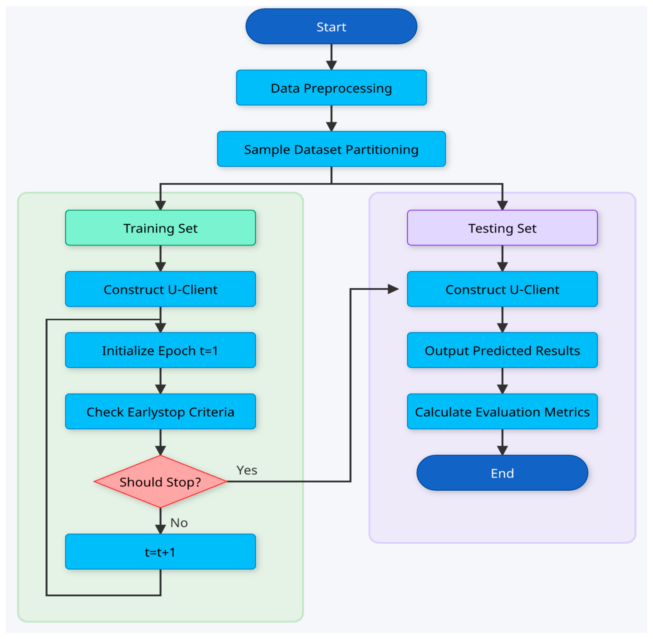
The overall forecasting framework of the proposed U-Client model is illustrated in Figure 5. The forecasting process mainly consists of four stages: data preprocessing, feature selection, spatio-temporal feature extraction, and forecasting output generation.

Figure 5. Forecasting flowchart.

Step 1: Raw photovoltaic power data and meteorological data are collected from the PV power station. Subsequently, Pearson correlation analysis is employed to evaluate the correlation between meteorological variables and PV power output. Meteorological factors with weak correlations are eliminated to reduce redundant information and improve computational efficiency.

Step 2: The selected historical PV power sequences and meteorological feature sequences are fed into the proposed U-Client model. The model adopts parallel cross-temporal attention and cross-variable attention branches to simultaneously extract temporal dependency information and variable interaction information.

Step 3: The outputs of the two attention branches are adaptively fused through a gated fusion mechanism.

Step 4: The fused features are combined with the linear projection module to generate the final forecasting results. The predicted PV power values are then compared with the actual measured values using evaluation metrics to evaluate the forecasting performance of the proposed model.

To evaluate forecasting performance, this paper employs Root Mean Square Error (RMSE), Mean Absolute Error (MAE), and Mean Absolute Percentage Error (MAPE). Their definitions are given as follows:

$$\mathrm{RMSE}=\sqrt{{\displaystyle \frac{1}{n}}{\displaystyle \sum _{i=1}^n{\left({\widehat{y}}_i-y_i\right)}^2}}$$

(10)

$$\mathrm{MAE}={\displaystyle \frac{1}{n}}{\displaystyle \sum _{i=1}^n\left|{\widehat{y}}_i-y_i\right|}$$

(11)

$$\mathrm{MAPE}={\displaystyle \frac{1}{n}}{\displaystyle \sum _{i=1}^n\left|\frac{{\widehat{y}}_i-y_i}{y_i}\times 100\%\right|}$$

(12)

where ${\widehat{y}}_i$ represents the actual power value; $y_i$ represents the predicted power value; and $n$ represents the number of samples.

5. Case Study and Analysis

To verify the effectiveness of the proposed forecasting framework, measured photovoltaic power and corresponding meteorological data from a 50 MW PV power station in Ningxia, China, covering the whole year of 2025, were employed as the experimental dataset. The dataset contains 35,040 daytime sampling points collected throughout 2025 with a sampling interval of 15 min. The training set, validation set and testing set were divided at a ratio of 70:15:15. In addition, several benchmark forecasting models were established for comparative analysis.

5.1. Feature Selection

The magnitude of photovoltaic power generation depends heavily on meteorological factors. This paper analyzes 18 meteorological variables from a 50 MW photovoltaic power plant in Ningxia, China, for the entire year of 2025. The raw power output is recorded in kilowatts (kW). Considering the 15 min sampling interval, the dataset comprises 35,040 time steps. With an input window length of 96 and a maximum forecasting horizon of four steps, the effective sample size is 34,940. The dataset is partitioned chronologically into a training set (70%), a validation set (15%), and a testing set (15%), yielding 24,458 training samples, 5241 validation samples, and 5241 testing samples.

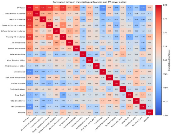
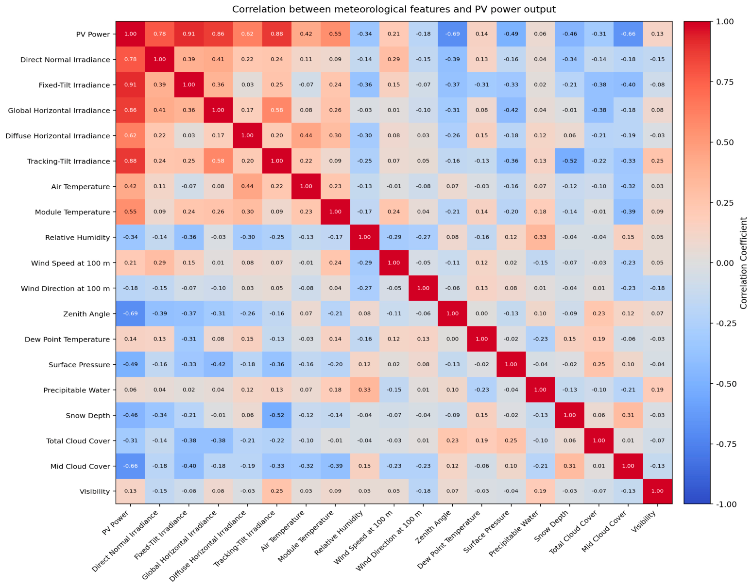
First, the Pearson correlation coefficient between actual power output and meteorological characteristics was calculated to perform an initial selection of feature data [31]. A larger absolute value of the coefficient indicates a stronger correlation between the two variables. The calculation formula is shown in Equation (13), and the heatmap illustrating the correlation between meteorological characteristics and photovoltaic power output is shown in Figure 6. This heatmap has been regenerated so that the variable set, variable names, and wind height (100 m) are fully consistent with the feature list in the text; the matrix is symmetric with a unit diagonal.

$$r={\displaystyle \frac{{\displaystyle \sum _{i=1}\left(x_i-\overline{x}\right)}\left(y_i-\overline{y}\right)}{\sqrt{{\displaystyle \sum _{i=1}{\left(x_i-\overline{x}\right)}^2}{\displaystyle \sum _{i=1}{\left(y_i-\overline{y}\right)}^2}}}}$$

(13)

where $r$ is the correlation coefficient; $x_i$ and $y_i$ represent the sample values of the two variables; and $\overline{x}$ and $\overline{y}$ represent the sample means of the corresponding variables.

Figure 6. Thermal map of the correlation between meteorological features and PV power.

The correlation analysis results indicate that direct normal irradiance, fixed-tilt irradiance, global horizontal irradiance, and tracking-tilt irradiance exhibit the strongest correlations with photovoltaic power output. To balance computational efficiency and information retention, a strict numeric threshold of |r| > 0.15 was applied for feature inclusion. Variables with correlation coefficients below this threshold—including snow depth, cloud cover, and surface pressure—were excluded from the input dataset. The final selected feature set consists of 10 variables: Direct Normal Irradiance, Fixed-tilt Irradiance, Global Horizontal Irradiance, Diffuse Horizontal Irradiance, Air Temperature, Module Temperature, Relative Humidity, Wind Speed at 100 m, Wind Direction at 100 m, and Zenith Angle.

After feature selection, the dimensionality of the input data is effectively reduced while retaining the most influential meteorological information. This process not only improves computational efficiency but also alleviates the influence of redundant variables on forecasting accuracy.

5.2. Parameter Settings and Training Environment

To ensure the objectivity and reproducibility of the experiments, the main parameters of the proposed model were determined through a trial-and-error approach. After testing multiple parameter combinations, the final parameter settings of the forecasting model are listed in Table 1.

Table 1. Parameters of the predictive model.

Parameter	Value
Input observation window	96
Forecast horizon	1–4
Batch size	64
Learning rate	0.001
Epoch	500
Dropout	0.1
Training iterations	100
Number of heads	4
Optimizer	Adam

The network training was intentionally conducted in a CPU-only environment to demonstrate the computational efficiency and lightweight nature of the proposed U-Client model. This design choice also demonstrates the model’s suitability for deployment in resource-constrained edge computing devices at PV power stations, where dedicated GPU resources may not be available. The hardware and software configurations used in the experiments were as follows: CPU: 12th Gen Intel(R) Core(TM) i5-12400F 2.50 GHz; RAM: 32 GB; Operating System: Windows 11; Programming Language: Python 3.9; Deep Learning Framework: PyTorch 2.0. During the training stage, an early stopping strategy was adopted to reduce the risk of overfitting. Specifically, if the loss value did not decrease for 10 consecutive training epochs, the training process was terminated in advance.

5.3. Forecasting Results of Comparative Models

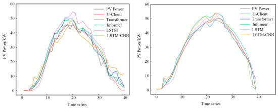
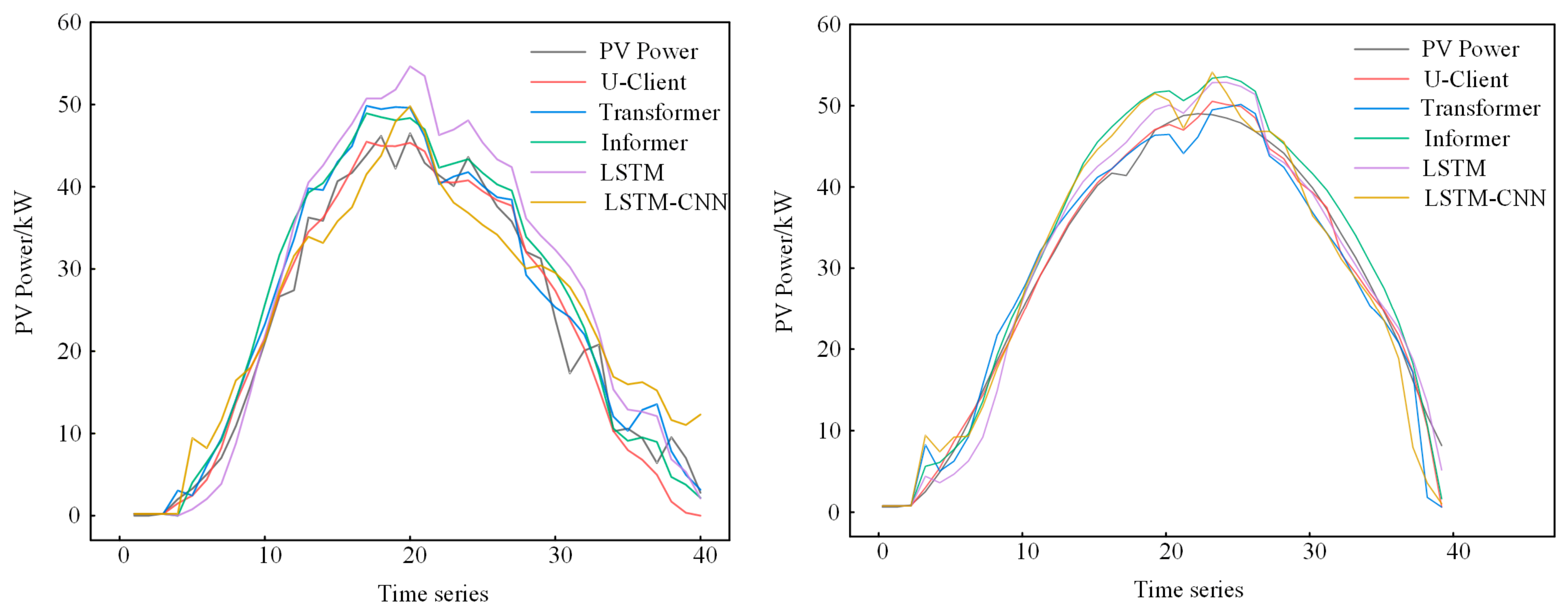
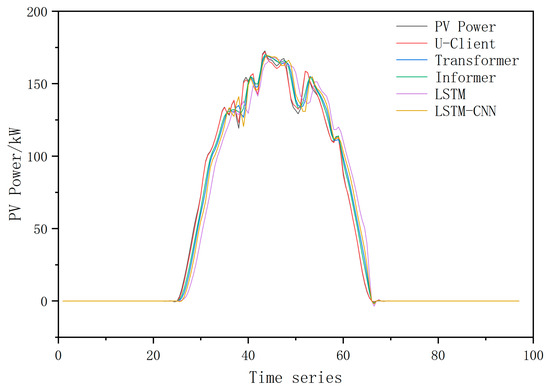
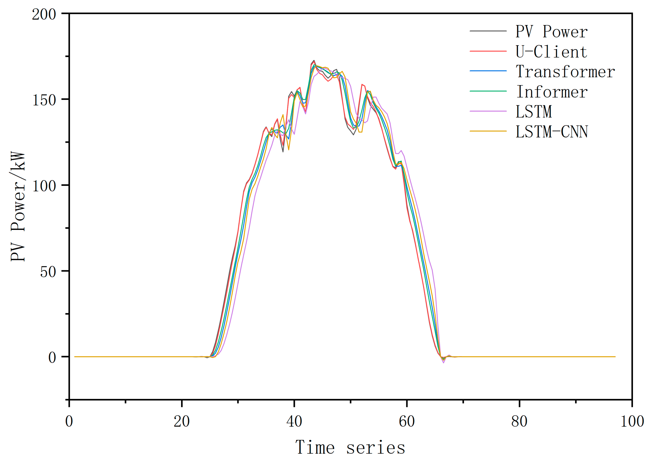
To ensure statistical robustness, all models were trained and evaluated over five independent runs with different random seeds (seeds = 0, 1, 2, 3, 4). Table 2 represents the mean ± standard deviation across these five runs. To evaluate the predictive performance of the U-Client model, this section presents comparative experiments between it and four classic time-series forecasting models: LSTM, LSTM-CNN, Informer, and Transformer. Figure 7 visualizes the forecast curves for each model under cloudy and sunny conditions, respectively, to provide an intuitive comparison of the models’ forecasting performance under different weather conditions.

Table 2. Comparative model evaluation metric results.

Model	Steps	RMSE	MAE	MAPE
U-Client	1	2.598 ± 0.184	1.796 ± 0.144	13.590 ± 1.538
	2	3.099 ± 0.223	2.067 ± 0.156	14.290 ± 1.184
	3	3.699 ± 0.172	2.490 ± 0.189	17.190 ± 1.490
	4	4.248 ± 0.431	2.804 ± 0.108	19.060 ± 1.092
Transformer	1	3.167 ± 0.121	2.290 ± 0.236	16.330 ± 1.509
	2	3.786 ± 0.128	2.582 ± 0.306	18.660 ± 2.180
	3	4.276 ± 0.380	2.899 ± 0.248	21.230 ± 0.938
	4	4.682 ± 0.147	3.197 ± 0.248	23.030 ± 0.814
Informer	1	3.286 ± 0.155	2.109 ± 0.109	15.700 ± 0.514
	2	3.789 ± 0.272	2.464 ± 0.172	17.110 ± 1.811
	3	4.198 ± 0.322	2.667 ± 0.234	18.090 ± 1.356
	4	4.773 ± 0.428	2.894 ± 0.206	19.490 ± 1.073
LSTM	1	3.876 ± 0.464	2.898 ± 0.347	20.750 ± 2.192
	2	4.809 ± 0.451	3.456 ± 0.202	24.280 ± 1.230
	3	5.265 ± 0.295	3.865 ± 0.140	25.760 ± 2.549
	4	6.099 ± 0.403	4.467 ± 0.474	28.180 ± 1.826
LSTM-CNN	1	3.754 ± 0.436	2.765 ± 0.294	17.350 ± 0.521
	2	4.387 ± 0.214	3.199 ± 0.358	20.260 ± 1.465
	3	4.990 ± 0.590	3.575 ± 0.235	24.400 ± 0.892
	4	5.354 ± 0.464	3.786 ± 0.379	25.900 ± 1.406

Figure 7. Comparison of model forecasting results for cloudy (left) and sunny (right) conditions.

In the 1–4-step forecasts, the U-Client achieved the lowest RMSE, MAE, and MAPE across all forecasting horizons. The performance advantage remained consistent as the forecasting horizon increased, indicating superior forecasting stability.

5.4. Ablation Study Results

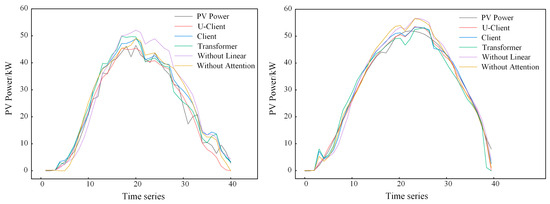
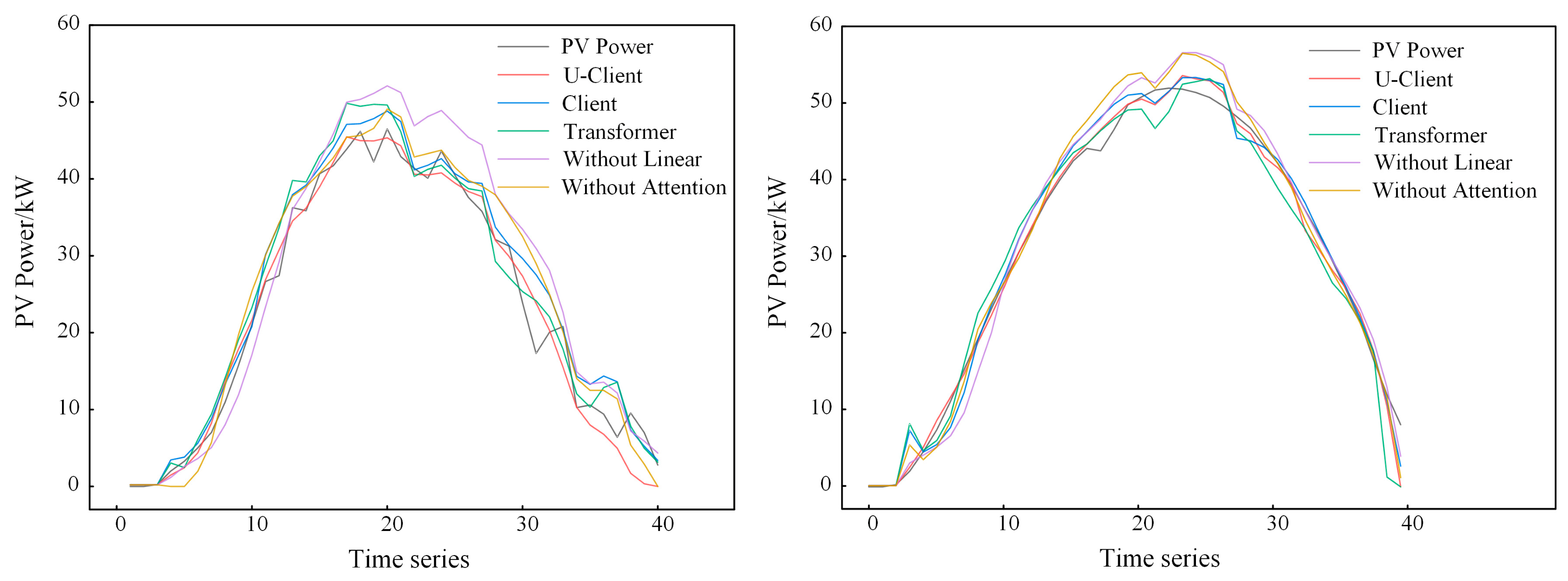
To further verify the effectiveness of each component in the proposed U-Client model, ablation experiments were conducted by comparing the complete U-Client model with the following variants, and the comparison results are presented in Table 3 and Figure 8.

Table 3. Ablation study evaluation metric results.

Model	Steps	RMSE	MAE	MAPE
U-Client	1	2.598 ± 0.098	1.796 ± 0.108	13.590 ± 1.587
	2	3.099 ± 0.304	2.067 ± 0.084	14.290 ± 0.746
	3	3.699 ± 0.145	2.490 ± 0.088	17.190 ± 1.749
	4	4.248 ± 0.195	2.804 ± 0.225	19.060 ± 1.339
Client	1	3.111 ± 0.147	2.043 ± 0.196	15.680 ± 0.655
	2	3.786 ± 0.333	2.497 ± 0.101	18.040 ± 1.224
	3	4.126 ± 0.203	2.657 ± 0.144	19.060 ± 2.237
	4	4.756 ± 0.487	3.009 ± 0.173	20.370 ± 2.233
Transformer	1	3.167 ± 0.155	2.290 ± 0.150	16.330 ± 1.746
	2	3.786 ± 0.332	2.582 ± 0.101	18.660 ± 2.221
	3	4.276 ± 0.210	2.899 ± 0.154	21.230 ± 2.113
	4	4.682 ± 0.279	3.197 ± 0.181	23.030 ± 0.843
U-Client without the linear module	1	3.298 ± 0.126	2.167 ± 0.179	16.760 ± 0.869
	2	3.875 ± 0.326	2.598 ± 0.165	18.760 ± 1.328
	3	4.357 ± 0.507	3.011 ± 0.221	21.460 ± 1.754
	4	4.653 ± 0.502	3.054 ± 0.142	21.530 ± 0.945
U-Client without the improved attention mechanism	1	3.287 ± 0.367	2.199 ± 0.228	16.160 ± 0.848
	2	3.789 ± 0.178	2.264 ± 0.219	16.660 ± 1.910
	3	4.197 ± 0.200	2.635 ± 0.304	19.260 ± 2.107
	4	4.468 ± 0.377	3.099 ± 0.211	21.360 ± 0.840

Figure 8. Comparison of ablation experiments under cloudy (left) and sunny (right) conditions.

(1)

Client, representing the original Client model without the gated spatio-temporal joint attention mechanism;

(2)

Transformer;

(3)

U-Client without the linear module;

(4)

U-Client without the improved attention mechanism.

The experimental results demonstrate that the complete U-Client model achieves superior forecasting performance across all forecasting horizons compared with the original Client model, thereby validating the effectiveness of the proposed gated spatio-temporal joint attention mechanism.

5.5. Computational Cost and Efficiency Analysis

To evaluate the practical deployment feasibility of the proposed U-Client model, a quantitative comparison of computational costs among all evaluated models is presented in Table 4. All experiments were conducted in the CPU environment described in Section 5.2.

Table 4. Quantitative comparison of computational costs.

Model	Parameters (K)	Training Time (s/Epoch)	Inference Time (ms/Sample)	Memory (MB)
LSTM	82	12.4	1.8	45
LSTM-CNN	95	14.2	2.1	52
Client	106	18.7	2.5	78
Transformer	118	22.5	2.8	86
Informer	142	28.3	3.5	104
U-Client (Ours)	125	24.1	3.2	92

As shown in Table 4, the U-Client model has approximately 125K trainable parameters, which is moderately higher than LSTM (82K) and the original Client (106K), but lower than Informer (142K) and comparable to the standard Transformer (118K). The average inference time per sample is only 3.2 ms. Given that the forecasting interval of the PV power station is 15 min (900,000 ms), the inference speed is orders of magnitude faster than the required response time, fully confirming the feasibility of real-time deployment even on resource-constrained edge devices without GPU acceleration. The memory footprint of 92 MB is well within the capacity of modern embedded systems and industrial computers commonly deployed at PV stations.

5.6. Hyperparameter Sensitivity Analysis

To evaluate the robustness of the proposed model to hyperparameter choices, a systematic sensitivity analysis was conducted on three key hyperparameters: (1) the input observation window length L ∈ {12, 24, 48, 96} steps, (2) the number of attention heads h ∈ {2, 4, 8, 16}, and (3) the hidden dimension size d ∈ {32, 64, 128, 256}. Table 5 summarizes the MAPE results under different configurations.

Table 5. Hyperparameter sensitivity analysis results.

Hyperparameter	Value	1-Step MAPE (%)	4-Step MAPE (%)
Window Length L	12	15.23	21.87
Window Length L	24	14.51	20.64
Window Length L	48	13.82	19.45
Window Length L	96 (default)	13.59	19.06
Attention Heads h	2	14.12	19.78
Attention Heads h	4 (default)	13.59	19.06
Attention Heads h	8	13.74	19.23
Attention Heads h	16	14.05	19.61
Hidden Dim d	32	14.38	20.12
Hidden Dim d	64 (default)	13.59	19.06
Hidden Dim d	128	13.67	19.15
Hidden Dim d	256	13.91	19.48

The results demonstrate that the model achieves optimal performance with the default configuration (L = 96, h = 4, d = 64). Across all tested ranges, the maximum MAPE fluctuation is 1.64% for one-step and 2.81% for four-step forecasting, indicating that the model is reasonably robust to moderate hyperparameter variations.

5.7. Statistical Significance Analysis

To rigorously verify whether the performance improvements achieved by the U-Client model are statistically significant, the Diebold-Mariano (DM) test was conducted on the 1-step forecasting residuals. The DM test evaluates the null hypothesis that two competing forecasts have equal predictive accuracy. Table 6 presents the DM test statistics and corresponding p-values for pairwise comparisons between U-Client and each baseline model.

Table 6. Diebold-Mariano (DM) test results for 1-step forecasting.

Compared Models	DM Statistic	p-Value
U-Client vs. LSTM	−4.82	<0.001
U-Client vs. LSTM-CNN	−4.15	<0.001
U-Client vs. Client	−2.94	0.0033
U-Client vs. Transformer	−3.28	0.0011
U-Client vs. Informer	−3.05	0.0023

Note: indicates significance at the 0.1% level; indicates significance at the 1% level. All p-values are well below the conventional 5% threshold, confirming that the performance improvements of U-Client over all baseline models are statistically significant and not attributable to random variation in the test data.

5.8. Validation on a Public Benchmark Dataset

To ensure reproducibility and demonstrate broader generalization, the proposed U-Client model was further validated on the public Desert Knowledge Australia Solar Centre (DKASC) benchmark dataset, which provides meteorological and PV power records that were aggregated to 15 min intervals to match the primary experimental setup.

Table 7 and Figure 9 present the forecasting results on the DKASC benchmark dataset. Consistent with the results obtained from the Ningxia dataset, U-Client achieves the best performance across all forecasting horizons and evaluation metrics. For one-step forecasting, U-Client obtains the lowest RMSE, MAE, and MAPE among all compared models. As the forecasting horizon increases, the errors of all models gradually rise; however, U-Client consistently maintains the lowest error growth rate. Even for four-step forecasting, its MAPE remains lower than those of Transformer, LSTM-CNN, and LSTM, demonstrating superior forecasting accuracy and stability on the public benchmark dataset.

Table 7. Comparative model evaluation metric results.

Model	Steps	RMSE	MAE	MAPE
U-Client	1	2.864 ± 0.173	1.952 ± 0.125	14.82 ± 1.16
	2	3.381 ± 0.201	2.253 ± 0.141	15.67 ± 1.24
	3	3.987 ± 0.246	2.641 ± 0.186	18.23 ± 1.37
	4	4.612 ± 0.292	3.014 ± 0.214	20.48 ± 1.55
Transformer	1	3.527 ± 0.196	2.289 ± 0.153	16.73 ± 1.32
	2	4.018 ± 0.215	2.587 ± 0.178	18.16 ± 1.48
	3	4.469 ± 0.284	2.872 ± 0.196	19.62 ± 1.66
	4	5.041 ± 0.325	3.168 ± 0.237	21.21 ± 1.74
Informer	1	3.618 ± 0.183	2.467 ± 0.162	17.42 ± 1.41
	2	4.219 ± 0.229	2.781 ± 0.187	19.36 ± 1.53
	3	4.698 ± 0.248	3.026 ± 0.194	21.04 ± 1.62
	4	5.214 ± 0.306	3.384 ± 0.228	22.91 ± 1.83
LSTM	1	4.106 ± 0.272	2.913 ± 0.204	18.91 ± 1.67
	2	4.756 ± 0.301	3.328 ± 0.225	21.14 ± 1.82
	3	5.397 ± 0.348	3.714 ± 0.248	24.06 ± 1.95
	4	5.881 ± 0.407	4.029 ± 0.283	25.73 ± 2.12
LSTM-CNN	1	4.312 ± 0.314	3.108 ± 0.225	21.96 ± 1.91
	2	5.296 ± 0.352	3.698 ± 0.274	25.17 ± 2.05
	3	5.882 ± 0.389	4.093 ± 0.301	27.13 ± 2.28
	4	6.714 ± 0.426	4.784 ± 0.337	29.87 ± 2.43

Figure 9. Comparison of model forecasting results for DKASC benchmark dataset.

6. Conclusions

In this paper, an improved Transformer-based photovoltaic power forecasting model termed U-Client is proposed to enhance the forecasting accuracy and stability of ultra-short-term PV power forecasting. On this basis, a gated spatio-temporal joint attention mechanism is constructed by integrating cross-temporal attention and cross-variable attention into the Client framework. The effectiveness of the proposed model is verified through comparative experiments and ablation studies. The main conclusions obtained from this study are summarized as follows:

(1)

The proposed U-Client model achieved the best forecasting accuracy across all forecasting horizons, outperforming LSTM, LSTM-CNN, Informer, and Transformer in RMSE, MAE, and MAPE.

(2)

The proposed spatio-temporal joint attention mechanism effectively captures temporal dependencies and variable interactions. The gating unit further improves feature utilization by adaptively fusing the two representations.

(3)

The feature selection strategy based on Pearson correlation analysis effectively reduces redundant meteorological information and improves computational efficiency. The selected meteorological variables with strong correlations provide reliable data support for the forecasting model. Meanwhile, the ablation study verifies that both the linear module and the proposed spatio-temporal joint attention mechanism contribute significantly to forecasting performance improvement, demonstrating the rationality and effectiveness of the proposed model architecture.

Several directions for future research are identified:

(1)

Exploring nonlinear feature selection methods such as mutual information or SHAP-based importance ranking;

(2)

Extending the model with a lightweight autoregressive decoder for longer forecasting horizons (e.g., 12–24 steps);

(3)

Incorporating robust mechanisms for handling missing data and extreme weather events.

References

- Liang, Z.; Yin, X.; Chung, C.Y.; Rayeem, S.K.; Chen, X.; Yang, H. Managing massive RES integration in hybrid microgrids: A data-driven quad-level approach with adjustable conservativeness. IEEE Trans. Ind. Inform. 2025, 21, 7698–7709. [Google Scholar]
- Ndalloka, Z.N.; Nair, H.V.; Alpert, S.; Schmid, C. Solar photovoltaic recycling strategies. Sol. Energy 2024, 270, 112379. [Google Scholar] [CrossRef] [Scilit]
- Liang, Z.; Chung, C.Y.; Wang, Q.; Chen, H.; Yang, H.; Wu, C. Fortifying renewable-dominant hybrid microgrids: A bi-directional converter based interconnection planning approach. Engineering 2025, 51, 130–143. [Google Scholar]
- Di Leo, P.; Ciocia, A.; Malgaroli, G.; Spertino, F. Advancements and challenges in photovoltaic power forecasting: A comprehensive review. Energies 2025, 18, 2108. [Google Scholar] [CrossRef] [Scilit]
- Zhou, H.; Luo, F.; Zhuang, H.; Weng, Z.; Gong, X.; Lin, Z. Attention multihop graph and multiscale convolutional fusion network for hyperspectral image classification. IEEE Trans. Geosci. Remote Sens. 2023, 61, 5508614. [Google Scholar] [CrossRef] [Scilit]
- Weng, H.; Hu, Y.; Liang, M.; Xi, J.; Yin, B. Optimizing bidding strategy in electricity market based on graph convolutional neural network and deep reinforcement learning. Appl. Energy 2025, 380, 124978. [Google Scholar]
- Huo, G.; Zhang, Y.; Wang, B.; Gao, J.; Hu, Y.; Yin, B. Hierarchical spatio–temporal graph convolutional networks and transformer network for traffic flow forecasting. IEEE Trans. Intell. Transp. Syst. 2023, 24, 3855–3867. [Google Scholar] [CrossRef] [Scilit]
- Dao, F.; Zeng, Y.; Qian, J. Fault diagnosis of hydro-turbine via the incorporation of bayesian algorithm optimized CNN-LSTM neural network. Energy 2024, 290, 130326. [Google Scholar]
- Pentsos, V.; Tragoudas, S.; Wibbenmeyer, J.; Khdeer, N. A hybrid LSTM-Transformer model for power load forecasting. IEEE Trans. Smart Grid 2025, 16, 2624–2634. [Google Scholar] [CrossRef] [Scilit]
- Wang, M.; Chen, C.; Huang, X.; Tian, L.; Xie, J.; Gao, Z.; Zhou, X.; Yan, J. Carbon emission evaluation for regional public institutions operation phase based on improved LightGBM and carbon emission efficiency ratio. Energy 2026, 351, 140748. [Google Scholar] [CrossRef] [Scilit]
- Gong, J.; Qu, Z.; Zhu, Z.; Xu, H.; Yang, Q. Ensemble models of TCN-LSTM-LightGBM based on ensemble learning methods for short-term electrical load forecasting. Energy 2025, 318, 134757. [Google Scholar]
- Zhu, X.; Wang, L.; Gu, J.; Wang, P.; Tang, J.; Hao, J.; Xiang, M.; Lu, Y.; Lu, X. Ultra-short-term PV prediction based on LSTM with a multi-head attention mechanism. J. Phys. Conf. Ser. 2023, 2428, 012013. [Google Scholar] [CrossRef] [Scilit]
- Gao, H.; Qiu, S.; Fang, J.; Ma, N.; Wang, J.; Cheng, K.; Wang, H.; Zhu, Y.; Hu, D.; Liu, H.; et al. Short-term prediction of PV power based on combined modal decomposition and NARX-LSTM-LightGBM. Sustainability 2023, 15, 8266. [Google Scholar] [CrossRef] [Scilit]
- Mohamad Radzi, P.N.L.; Mekhilef, S.; Mohamed Shah, N.; Akhter, M.N.; Seyedmahmoudian, M.; Stojcevski, A. Optimizing solar power forecasting with metaheuristic algorithms and deep learning models for photovoltaic grid connected systems. Sci. Rep. 2025, 15, 40045. [Google Scholar] [CrossRef] [Scilit] [PubMed]
- Li, P.; Zhou, K.; Lu, X.; Yang, S. A hybrid deep learning model for short-term PV power forecasting. Appl. Energy 2020, 259, 114216. [Google Scholar] [CrossRef] [Scilit]
- Zhang, F.; Wang, X.; Wu, M.; Hou, X.; Han, C.; Liu, Z. Optimization design of uncertain parameters for improving the stability of photovoltaic system. J. Power Sources 2022, 521, 230959. [Google Scholar] [CrossRef] [Scilit]
- Yu, J.; Li, X.; Yang, L.; Li, L.; Huang, Z.; Shen, K.; Yang, X.; Yang, X.; Xu, Z.; Zhang, D.; et al. Deep learning models for PV power forecasting: Review. Energies 2024, 17, 3973. [Google Scholar] [CrossRef] [Scilit]
- Alsamraee, S.A.; Khanna, S. A Hybrid Transformer–TCN–GRU Based Model for Thermal Load Forecasting of a Large University Campus. Energy 2026, 344, 140114. [Google Scholar]
- Cui, S.; Lyu, S.; Ma, Y.; Wang, K. Improved informer PV power short-term prediction model based on weather typing and AHA-VMD-MPE. Energy 2024, 307, 132766. [Google Scholar] [CrossRef] [Scilit]
- Ban, G.; Chen, Y.; Xiong, Z.; Zhuo, Y.; Huang, K. The univariate model for long-term wind speed forecasting based on wavelet soft threshold denoising and improved Autoformer. Energy 2024, 290, 130225. [Google Scholar] [CrossRef] [Scilit]
- Simeunović, J.; Schubnel, B.; Alet, P.-J.; Carrillo, R.E. Spatio-temporal graph neural networks for multi-site PV power forecasting. IEEE Trans. Sustain. Energy 2022, 13, 1210–1220. [Google Scholar] [CrossRef] [Scilit]
- Chen, Q.; Liu, Z.; Zhen, Z. Regional Short-Term PV Power Forecasting Based on Graph Convolution and Transformer Networks. Electronics 2026, 15, 1817. [Google Scholar] [CrossRef] [Scilit]
- Kim, J.; Kim, H.; Kim, H.G.; Lee, D.; Yoon, S. A comprehensive survey of deep learning for time series forecasting: Architectural diversity and open challenges. Artif. Intell. Rev. 2025, 58, 216. [Google Scholar] [CrossRef] [Scilit]
- Liu, Y.; Zhang, Y.; Wang, Y.; Hou, F.; Yuan, J.; Tian, J. A survey of visual transformers. IEEE Trans. Neural Netw. Learn. Syst. 2023, 35, 7478–7498. [Google Scholar] [CrossRef] [Scilit]
- Cai, C.; Zhang, L.; Zhou, J. DMPR: A novel wind speed forecasting model based on optimized decomposition, multi-objective feature selection, and patch-based RNN. Energy 2024, 310, 133277. [Google Scholar]
- Lu, Q.; Zeng, H.; Yin, L. Dynamic distributed multi-objective mantis search algorithm based on Transformer hybrid strategy for novel power system dispatch. Energy 2025, 324, 136075. [Google Scholar] [CrossRef] [Scilit]
- Gao, J.; Hu, W.; Zhang, D.; Chen, Y. Client: Cross-variable linear integrated enhanced transformer for multivariate long-term time series forecasting. AI Open 2025, 6, 93–107. [Google Scholar]
- Kim, T.; Kim, J.; Tae, Y.; Park, C.; Choi, J.H.; Choo, J. Reversible Instance Normalization for Accurate Time-Series Forecasting against Distribution Shift. In Proceedings of the International Conference on Learning Representations (ICLR), Virtual, 25–29 April 2022. [Google Scholar]
- Hu, L.; Tang, J.; Xu, F.; Liang, X. SOC prediction for electric buses based on interpretable transformer model: Impact of traffic conditions and feature importance. Energy 2025, 324, 135935. [Google Scholar] [CrossRef] [Scilit]
- Osolo, R.I.; Yang, Z.; Long, J. An Analysis of the Use of Feed-Forward Sub-Modules for Transformer-Based Image Captioning Tasks. Appl. Sci. 2021, 11, 11635. [Google Scholar] [CrossRef] [Scilit]
- Cao, T.; Xu, Y.; Liu, G.; Tao, S.; Tang, W.; Sun, H. Feature-enhanced deep learning method for electric vehicle charging demand probabilistic forecasting of charging station. Appl. Energy 2024, 371, 123751. [Google Scholar] [CrossRef] [Scilit]
Disclaimer/Publisher’s Note: The statements, opinions and data contained in all publications are solely those of the individual author(s) and contributor(s) and not of MDPI and/or the editor(s). MDPI and/or the editor(s) disclaim responsibility for any injury to people or property resulting from any ideas, methods, instructions or products referred to in the content. |
© 2026 by the authors. Licensee MDPI, Basel, Switzerland. This article is an open access article distributed under the terms and conditions of the Creative Commons Attribution (CC BY) license.