Research on Day-Ahead Electricity Price Forecasting Method for New Energy Power Market Based on Hyperparameter Adaptation

Abstract

The large-scale integration of wind and solar power introduces significant volatility into electricity markets, posing challenges for accurate day-ahead price forecasting for generation companies. This paper proposes a hybrid forecasting model, CEEMD-SE-IBA-LSTM, based on hyperparameter adaptation to improve prediction accuracy. First, a similar-day selection method integrating Random Forest and an Improved Grey Ideal Value approximation identifies the most relevant historical days. Second, Complete Ensemble Empirical Mode Decomposition with Sample Entropy (CEEMD-SE) decomposes and reconstructs the price series into stable components. Third, an Improved Bat Algorithm (IBA), incorporating differential evolution and adaptive weighting, is developed to optimize two key LSTM hyperparameters: the number of hidden layer neurons, which is treated as a model architecture hyperparameter, and the learning rate, which is treated as a training hyperparameter. The number of LSTM layers and the number of training epochs are kept fixed as model settings to ensure reproducibility. Using data from the US PJM market, the proposed model is validated against six benchmarks. The results show that CEEMD-SE-IBA-LSTM achieves superior performance, with a Mean Absolute Percentage Error (MAPE) of 3.73%, a Root Mean Square Error (RMSE) of 3.57 $/MWh, and a Mean Absolute Error (MAE) of 1.95 $/MWh. The method provides accurate price trends, offering effective decision support for new energy enterprises in price bidding to enhance revenue.

1. Introduction

As the global energy structure transitions towards a new power system dominated by renewable energy, the deepening of power market reforms and the accelerated construction of a market-oriented electricity system have become key development trends for power sectors in numerous countries worldwide [1]. The day-ahead market, as the core channel for electricity spot trading, sees its price trends directly impacting the interests of all stakeholders. Accurate day-ahead electricity price forecasting is therefore crucial for the bidding strategies of generation companies, consumption decisions of users, and the stable operation of the power grid [2]. However, the large-scale integration of renewable energy sources like wind and solar power complicates the supply-demand balance of the power system. Their inherent randomness and near-zero marginal cost characteristics exacerbate volatility in day-ahead prices, posing significant challenges to traditional forecasting methods [3,4]. Recent field evidence from politically unstable regions, such as the study by Lin et al. on decentralized solar PV systems for energy resilience under fragile-grid conditions [5], highlights the importance of considering real-world infrastructure changes, grid resilience, and renewable supply volatility, which further strengthens the need for accurate price forecasting in renewable-integrated electricity markets.

In current research on electricity market price forecasting, time series methods can stably output short-term predictions for stationary price data with significant trends and periodicity. Yet, their strong reliance on the assumption of data stationarity makes them difficult to adapt to the complex fluctuation patterns of electricity prices following high renewable energy integration [6,7,8,9]. Artificial intelligence methods demonstrate significant advantages in handling nonlinear and complex problems [10,11,12], but they suffer from issues such as slow convergence and susceptibility to local optima. Combined forecasting is a highly comprehensive approach that organically integrates multiple algorithms to enhance prediction accuracy and reliability [13,14,15]. Literature [16] proposed an electricity price forecasting model based on an Attention-optimized Gated Recurrent Unit (Attention-GRU). By utilizing the attention mechanism to clarify input features with greater influence on prices, it addressed the slow prediction speed problem of LSTM neural networks. Literature [17] applied wavelet packet decomposition to known electricity price sequences, removed invalid information from the decomposed components, and used an LSTM network to forecast the remaining useful information. Literature [18] considered geographical spatio-temporal factors, using information extracted by a Graph Convolutional Neural Network as input to a Long Short-Term Memory network, thereby improving prediction accuracy and generalizability through a combined model. Literature [19] proposed using Empirical Mode Decomposition (EMD) to decompose price sequences into periodic and trend components, constructing a combined forecasting model integrating LSTM and Support Vector Regression (SVR) to obtain predicted price sequences.

Although existing research has made certain progress, three core issues remain to be addressed under the scenario of high-penetration renewable energy integration into power markets. First, the impact of renewable energy factors on electricity prices has not been fully quantified, as most models merely incorporate wind and photovoltaic power generation data without an in-depth analysis of the intrinsic correlation between penetration indicators, such as wind-to-load ratio and photovoltaic share, and electricity prices. Second, there is insufficient synergy between data preprocessing and model optimization. Forecasting directly on highly volatile original price sequences makes it difficult for models to capture their underlying patterns. Although literature [20] employed EMD to process price sequences, it suffers from mode mixing problems, affecting subsequent prediction accuracy. Third, hyperparameters of deep learning models like LSTM mostly rely on empirical settings, lacking efficient adaptive optimization mechanisms. Traditional algorithms such as the Bat Algorithm (BA) and Particle Swarm Optimization (PSO) are prone to slow convergence or local optima when optimizing LSTM parameters, constraining further improvements in forecasting performance. The existence of these problems renders existing forecasting methods inadequate to meet the practical demand of power market participants for high-accuracy, high-stability price predictions. Building upon this foundation, this paper proposes a day-ahead electricity price forecasting model named CEEMD-SE-IBA-LSTM based on multi-information fusion. The main contributions of this paper are as follows:

A novel multi-feature system for renewable energy, encompassing 13 types of variables, is proposed. These data, including wind power generation, wind power forecast deviation, photovoltaic power generation, PV forecast deviation, thermal power generation, total generation, actual power load, load forecast deviation, historical electricity prices, coal prices, and regional meteorological data, are collected from wind farm production management systems and publicly available information from regional trading centers. For the first time, derived variables are utilized as renewable energy penetration indicators to quantify their correlation with day-ahead prices. A novel electricity price forecasting method based on CEEMD-SE-IBA-LSTM is proposed. Firstly, CEEMD is used to decompose the electricity price time series into multiple IMF components and one residual component. Then, SE is applied to reconstruct the multiple subsequences obtained from decomposition, thereby reducing data noise while decreasing the model’s computational load. Subsequently, an Improved Bat Algorithm is employed to optimize two key LSTM hyperparameters, namely the number of hidden layer neurons and the learning rate, thereby constructing an IBA-LSTM prediction model. Finally, the multiple components from high to low frequency for the day preceding the target forecast day, obtained via the combined CEEMD-SE data preprocessing strategy, are input into the IBA-LSTM models. Regression predictions are performed separately on each reconstructed subsequence. After denormalization, the prediction results are integrated to ultimately obtain the forecasted spot electricity market price.

2. Materials and Methods

2.1. Analysis of Day-Ahead Price Influencing Factors and Similar-Day Selection

2.1.1. Analysis of Day-Ahead Price Characteristics

This paper selects the US PJM electricity market, known for its high data completeness and accuracy, as the subject for empirical analysis. The original dataset includes nine variables: Load (D); Load Forecast Error (De); Thermal Power Generation (TP); Wind Power Generation (W); Wind Power Forecast Error (We); Photovoltaic Power Generation (S); PV Forecast Error (Se); Total Generation (L); and Historical Electricity Price (P). To better characterize the impact of new energy penetration, four derived indicators are added, Wind-to-Load Ratio (WD); PV-to-Load Ratio (SD); Wind Power Proportion (RW); and PV Power Proportion (RS), forming a 13-dimensional feature vector.

The Pearson Correlation Coefficient (PCC) is calculated to quantify the correlation between each element and the electricity price [19]. For two variables $X=(x_1,x_2,\cdots x_n)$ and $Y=(y_1,y_2,\cdots y_n)$, $PCC(X,Y)$ is given by:

$$PCC(X,Y)={\displaystyle \frac{{\displaystyle \sum _{i=1}^n(x_i-\overline{x_i})}(y_i-\overline{y_i})}{\sqrt{{\displaystyle \sum _{i=1}^n{(x_i-\overline{x_i})}^2}}{\displaystyle \sum _{i=1}^n\sqrt{{\left(y_i-\overline{y_i}\right)}^2}}}}$$

(1)

where $\overline{x_i}$ is the mean of $x_i$, and $\overline{y_i}$ is the mean of $y_i$. The specific Pearson Correlation Coefficient values for the aforementioned influencing factors are shown in Table 1.

Table 1. Results of correlation analysis between factors and day-ahead electricity price.

Influencing Factor	PCC (X, Y)
Actual Load	0.519
Load Forecast Error	0.401
Thermal Power Generation	0.107
Wind Power Generation	−0.223
Wind Power Forecast Error	0.439
Photovoltaic Power Generation	−0.356
PV Forecast Error	0.611
Total Generation	−0.105
Historical Price	0.681
Wind-to-Load Ratio	−0.563
PV-to-Load Ratio	−0.642
Wind Power Proportion	−0.821
PV Power Proportion	−0.945

To clearly define the four derived renewable energy penetration indicators, the definitions are as follows: Wind-to-Load Ratio (WD) = Wind Power Generation (W)/Actual Load (D), PV-to-Load Ratio (SD) = Photovoltaic Power Generation (S)/Actual Load (D), Wind Power Proportion (RW) = Wind Power Generation (W)/Total Generation (L), PV Power Proportion (RS) = Photovoltaic Power Generation (S)/Total Generation (L).

The results show that PV Power Proportion (RS, PCC = −0.945) and Wind Power Proportion (RW, PCC = −0.821) exhibit strong negative correlations with the electricity price, while Historical Price (P, PCC = 0.681) and PV Forecast Error (Se, PCC = 0.611) show positive correlations. This indicates that new energy factors have a significant impact on electricity prices and must be fully considered in forecasting models.

2.1.2. Similar-Day Selection and Feature Fusion Based on RF-IAGIV

The systematic analysis of day-ahead price influencing factors clarifies the core roles of new energy penetration indicators and traditional factors, and verifies the existence of non-linear relationships and multicollinearity among factors. To accurately extract historical data with price patterns similar to the target forecast day, reduce interference from redundant information, and enhance the weight of core features, this study employs a Random Forest (RF) algorithm to quantify the influence degree of each factor on the day-ahead price, builds a quantitative model for the impact of new energy on prices, and eliminates less influential variables.

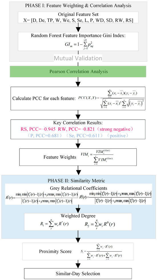
Traditional Grey Relational Analysis alone can only measure the trend similarity of features but cannot quantify their inherent importance, which may lead to interference from redundant features and degrade training data quality. This paper proposes an RF-IAGIV similar-day selection method [21]. First, Random Forest (RF) quantifies the importance of each feature to price similarity. The Gini coefficient is used to assess feature importance: multiple decision trees are constructed, and the Gini index for a node t is calculated as:

$$G{I}_m=1-{\displaystyle \sum _{j=1}^{\left|J\right|}}{p}_{mj}^2$$

(2)

where $G{I}_m$ is the Gini coefficient of node $m$ in the decision tree, $p_{mj}$ is the proportion of the $j$-th class of data in node $m$, and $\left|J\right|$ is the total number of data classes. The total Gini coefficient contribution of each feature is normalized by Equation (3) to quantify the influence degree of each factor on electricity price.

$$VI{M}_i={\displaystyle \frac{VI{M}_i^{(Gini)}}{{\displaystyle \sum _{i=1}^{i}V}I{M}_i^{(Gini)}}}$$

(3)

$VI{M}_i$ is the weight of the $i$-th factor, $VI{M}_i^{(Gini)}$ is the total Gini coefficient contribution of the $i$-th factor, and $i$ is the total number of core factors after screening. The Gini coefficient contribution of each factor is calculated through multiple decision trees, and core factors are screened from high to low by weight.

Normalize the feature importance scores calculated by random forest as the weight $w_r$ of each feature. Combined with the Improved Grey Ideal Value Approximation (IAGIV), the feature weights are integrated into similarity calculation to construct the “weighted grey relational closeness” index [22,23,24,25], realizing the accurate screening of “prioritizing important features and weakening redundant features”. The IAGIV method integrates grey relational analysis with TOPSIS. Let the set of historical days be $S=\{s_1,s_2,\dots ,s_N\}$, and the feature vector for each day be $X_k=\left[X_k(1),X_k(2),\dots ,X_k(c)\right]$. The optimal reference sequence $X^{\ast }$ consists of the best values of each feature across all historical days, while the worst reference sequence $X^0$ consists of the worst values. The grey relational coefficients of the $r$-th feature of the $k$-th historical day with respect to the optimal and worst sequences are calculated as:

$${R_k}^{*}(r)={\displaystyle \frac{{\min }_k\min \left|X^{*}(r)-X(r)\right|+\rho {\max }_r\max \left|X^{*}(r)-X(r)\right|}{\left|X^{*}(r)-X(r)\right|+\rho {\max }_r\max \left|X^{*}(r)-X(r)\right|}}$$

(4)

$${R_k}^0(r)={\displaystyle \frac{{\min }_r\min \left|X^0(r)-X(r)\right|+\rho {\max }_r\max \left|X^0(r)-X(r)\right|}{\left|X^0(r)-X(r)\right|+\rho {\max }_r\max \left|X^0(r)-X(r)\right|}}$$

(5)

where $\rho$ is the distinguishing coefficient, which is generally set to 0.5 in grey relational analysis.

Calculate the grey relational coefficients ${R_k}^{*}(r)$ and ${R_k}^0(r)$ of the $r$-th core factor of the historical day with the optimal reference sequence and the worst reference respectively, and calculate the final grey relational closeness $S_k$:

$$S_k={\displaystyle \frac{{\displaystyle \sum _{r=1}^c{w}_r}·{R_k}^{*}(r)}{{\displaystyle {\displaystyle \sum _{r=1}^c}{w}_r}·{R_k}^{*}(r)+{\displaystyle {\displaystyle \sum _{r=1}^c}{w}_r}·{R_k}^0(r)}}$$

(6)

The closer the value of $S_k$ is to 1, the more similar the historical day is to the predicted day. The top 20 historical days with the highest similarity are selected to form the training set in order to realize the effective integration of multi-source information and the improvement of data quality. This paper uses RF-IAGIV for similar-day screening, and its flowchart is shown in Figure 1.

Figure 1. Framework of RF-IAGIV Similar-Day Selection Algorithm.

According to the aforementioned similar-day selection method, the similarity between each historical day and the forecast day is calculated and sorted in descending order. After screening similar days for different forecast days, it is found that historical days with high similarity are mainly concentrated within the 20 days preceding the forecast day, with similarities all exceeding 0.80, after which the similarity drops significantly. The top 20 ranked days and their similarities are listed in Table 2.

Table 2. The historical date and similarity of the top 20 similarity rankings.

Rank	Date	Similarity	Rank	Date	Similarity
1	8.12	0.954	11	6.29	0.863
2	7.29	0.949	12	4.17	0.857
3	8.1	0.942	13	6.8	0.844
4	5.2	0.933	14	5.11	0.835
5	6.25	0.921	15	5.6	0.831
6	8.7	0.914	16	5.23	0.827
7	8.30	0.905	17	6.26	0.821
8	8.17	0.902	18	6.27	0.814
9	6.30	0.887	19	7.3	0.812
10	7.27	0.874	20	7.18	0.801

2.2. Methodologies

2.2.1. Decomposition and Reconstruction of Original Price Time Series Based on CEEMD-SE

After obtaining a high-quality similar-day training set, it is necessary to further preprocess the volatile electricity price series. To reduce the non-stationarity and noise of the original electricity price series, this paper adopts Complete Ensemble Empirical Mode Decomposition for adaptive decomposition of the series. By introducing paired positive and negative white noise, CEEMD effectively solves the mode mixing problem of traditional EMD [26]. When performing modal decomposition on the original electricity price series, obtaining into k $I_{M{F}_i}$ and a residual term $R$.

$$P(t)={\displaystyle \sum _{i=1}^k}{I}_{M{F}_i}+R(t)$$

(7)

where $k$ is the total number of IMF components. After performing modal decomposition using the CEEMD method, $n$ sub-modal components will be generated. If a prediction model is built for each component separately, the computational complexity will increase significantly. To solve this problem, the SE theory can be introduced for modal component optimization. The SE theory was proposed by Richman in 2000 [27], and its core lies in evaluating the complexity of the system by quantifying the probability of new pattern generation in the time series. The smaller the SE value, the stronger the self-similarity of the series and the more stable the system state. For a series with length $N$, its sample entropy is:

$$SamEn(m,r,N)=-\ln \left[{\displaystyle \frac{A^m(r)}{B^m(r)}}\right]$$

(8)

where $m$ is the embedding dimension, representing the vector dimension of the reconstructed sequence, and its value is set to 2 in this paper. $r$ is the similarity tolerance, which is used to judge whether two reconstructed vectors are similar patterns, and its value is set to 0.2 in this paper; $B^m(r)$ is the logarithmic average probability that the distance between any two m-dimensional reconstructed vectors is less than $r$. $A^m(r)$ is the logarithmic average probability that the distance between any two (m + 1)-dimensional reconstructed vectors is less than $r$.

2.2.2. LSTM Parameter Optimization Based on Improved Bat Algorithm

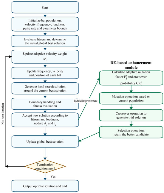
This paper proposes an Improved Bat Algorithm. Firstly, the Differential Evolution (DE) algorithm is integrated with Bat Algorithm. The current population is regarded as the initial population of DE, and mutation-crossover-selection operations are performed to improve population diversity. This process can effectively help the algorithm jump out of local optima [28,29]. Then, an adaptive weight parameter ${\omega }^t$ is introduced into the velocity update formula, and its update rule is consistent with the adaptive idea of DE parameters to balance the global exploration and local exploitation capabilities. The improved velocity update formula is as follows:

$${\omega }_i^t={\omega }_{\max }-e^{{\left({\displaystyle \frac{-5t}{t_{\max }}}\right)}^2}\left({\omega }_{\max }-{\omega }_{\min }\right)$$

(9)

$$v_i^t={\omega }_i^t{v}_i^{t-1}+f_i(x_i^t-x^{\ast })$$

(10)

In the formulas, ${\omega }_i^t$ represents the adaptive weight parameter of the $i$-th individual at the $t$-th iteration. ${\omega }_{\max }$ and ${\omega }_{\min }$ are the upper and lower limits of the velocity weight, respectively. $t$ is the current iteration number, and $t_{\max }$ is the maximum number of iterations set by the algorithm.

The probability density function (PDF) and cumulative distribution function (CDF) of the Cauchy distribution are used to construct the adaptive mutation factor $F_i^t$ and crossover probability $C_i^t$.

$$F_i^t=F_{\min }+(F_{\max }-F_{\min }){\displaystyle \frac{t-1}{T_{\max }}}+{\displaystyle \frac{\delta }{\pi }}\left[{\displaystyle \frac{{\theta }_1}{{(t-x_0)}^2+{\theta }_1^2}}\right]$$

(11)

$$C_i^t=\left(C_{\max }-C_{\min }\right)e^{\left(1-{\displaystyle \frac{t_{\max }}{t+1}}\right)}·\left[{\displaystyle \frac{1}{\pi }}\arctan \left({\displaystyle \frac{t-x_0}{{\theta }_2}}\right)+{\displaystyle \frac{1}{2}}\right]$$

(12)

where $F_i^t$ is the mutation factor of the $i$-th individual at the $t$-th iteration; $F_{\max }$ is the maximum mutation factor, and $F_{\min }$ is the minimum mutation factor. $t$ is the current iteration number; $t_{\max }$ is the maximum number of iterations. $\delta$ is a regulation factor; $x_0$ is the location parameter of the Cauchy distribution function, and ${\theta }_1$ is the scale parameter of the Cauchy distribution function. $C_i^t$ is the crossover probability of the $i$-th individual at the $t$-th iteration; $C_{\max }$ is the upper limit of the crossover probability, and $C_{\min }$ is the lower limit of the crossover probability. $t$ is the current iteration number; $t_{\max }$ is the maximum number of iterations of the algorithm. $x_0$ is the location parameter of the Cauchy cumulative distribution function, and ${\theta }_2$ is the scale parameter of the Cauchy cumulative distribution function. By adaptively adjusting the mutation factor $F$ and the crossover factor $c$ the convergence speed and precision of the algorithm can be effectively balanced, achieving a dual improvement in optimization performance. In the early stage of algorithm iteration, since the population is randomly distributed in the search space, larger $F$ values and smaller $C$ values should be set at this time to optimize the global search performance and accelerate the convergence process. However, in the later stage of iteration, when approaching the optimal solution, it is necessary to appropriately reduce the $F$ value and increase the $C$ value to enhance the local search performance and ensure a highly reliable convergence result. The adaptive velocity weight in this study is designed as an iteration-stage control factor. Its main purpose is to gradually adjust the search behavior from global exploration in the early stage to local exploitation in the later stage. Therefore, the exponential term is expressed as a function of the current iteration number and the maximum number of iterations. It should be noted that the adaptivity of the proposed IBA does not rely only on the velocity weight. The adaptive mutation factor and crossover probability constructed from the Cauchy distribution, together with the DE-based mutation, crossover, and selection operations, further adjust the population search behavior and retain individuals with better fitness values. Thus, the proposed IBA combines iteration-stage adaptation and fitness-based selection to improve convergence speed and optimization accuracy. The specific flow chart of the IBA proposed in this paper is shown in Figure 2.

Figure 2. The improved bat algorithm (IBA) structure diagram.

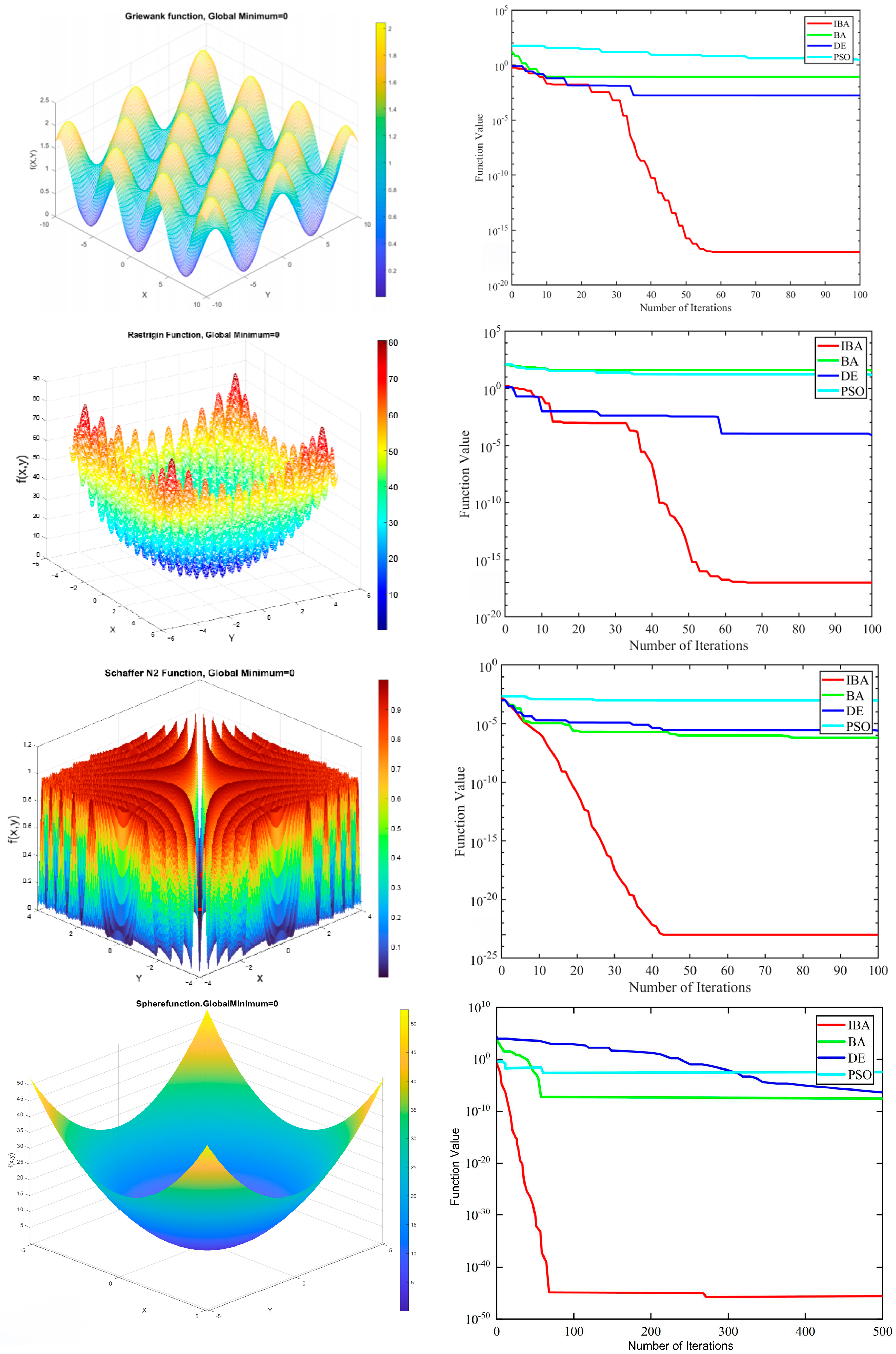
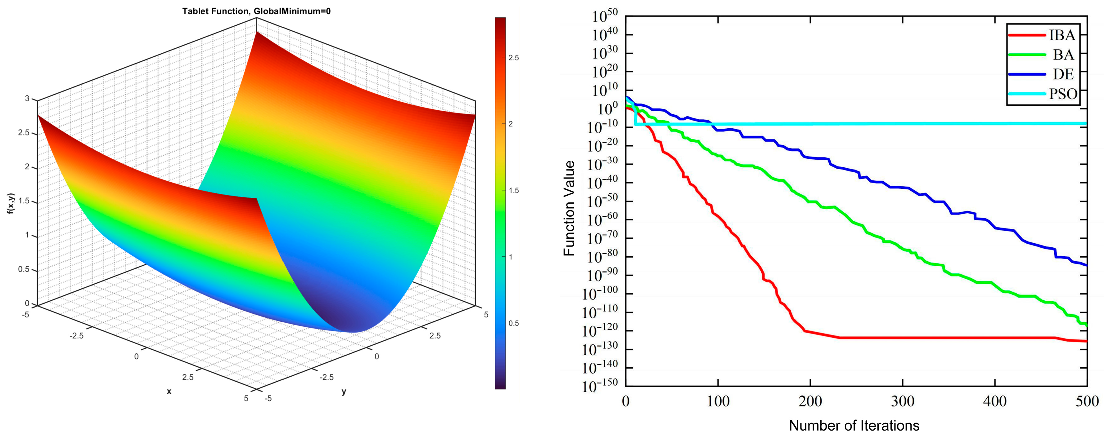
Six classical standard test functions are selected in this paper to test the performance of the improved bat algorithm, so as to evaluate the parameter optimization capability of the proposed IBA. Meanwhile, a comparative analysis is conducted between the IBA and the original BA, the differential evolution algorithm, as well as the PSO, which has exhibited excellent performance and been widely applied in recent years.

Each test function was independently run 20 times, and the global optimal value, worst value, and mean value were recorded. The detailed data comparison is shown in Table 3.

Table 3. Test function optimization results comparison.

Function		DE	PSO	BA	IBA
Ackley	Best	1.3288 × 10−7	1.9835	0.020389	8.8818 × 10−16
	Worst	0.0056875	9.6733	0.95735	4.3785 × 10−15
	Avg	3.9653 × 10−4	5.4939	0.035669	7.5943 × 10−15
Griewank	Best	1.2187 × 10−4	1.0581	0.10339	0
	Worst	0.012226	18.387	6.4805	0
	Avg	0.0071443	4.8853	0.57433	0
Rastrigin	Best	3.5319 × 10−4	26.969	9.1329	0
	Worst	0.085773	40.641	44.290	3.2294 × 10−11
	Avg	2.0579 × 10−5	36.866	24.448	1.6147 × 10−12
Schaffer N2	Best	2.0578 × 10−5	0.012772	9.8641 × 10−5	0
	Worst	0.0035895	18.386	8.0806	0
	Avg	1.8052 × 10−4	9.7361	4.0433	0
Sphere	Best	1.0455 × 10−12	1.6975 × 10−6	7.3562 × 10−7	5.7262 × 10−292
	Worst	2.0522 × 10−9	0.0055898	2.2213 × 10−5	3.9774 × 10−45
	Avg	4.2354 × 10−11	2.7963 × 10−4	3.2159 × 10−6	5.7928 × 10−46
Tablet	Best	4.4341 × 10−87	1.0531 × 10−9	6.2180 × 10−121	5.6421 × 10−176
	Worst	3.1163 × 10−80	1.0612 × 10−16	2.1664 × 10−115	8.0704 × 10−122
	Avg	8.3785 × 10−81	1.5877 × 10−10	6.6486 × 10−116	5.0913 × 10−123

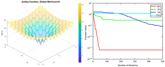
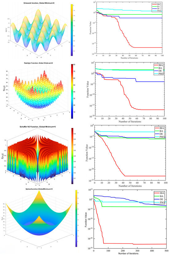
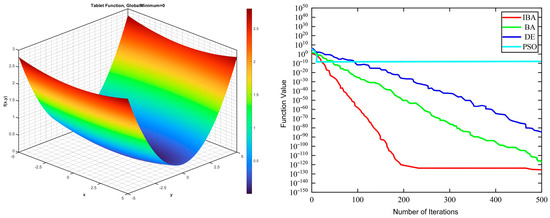
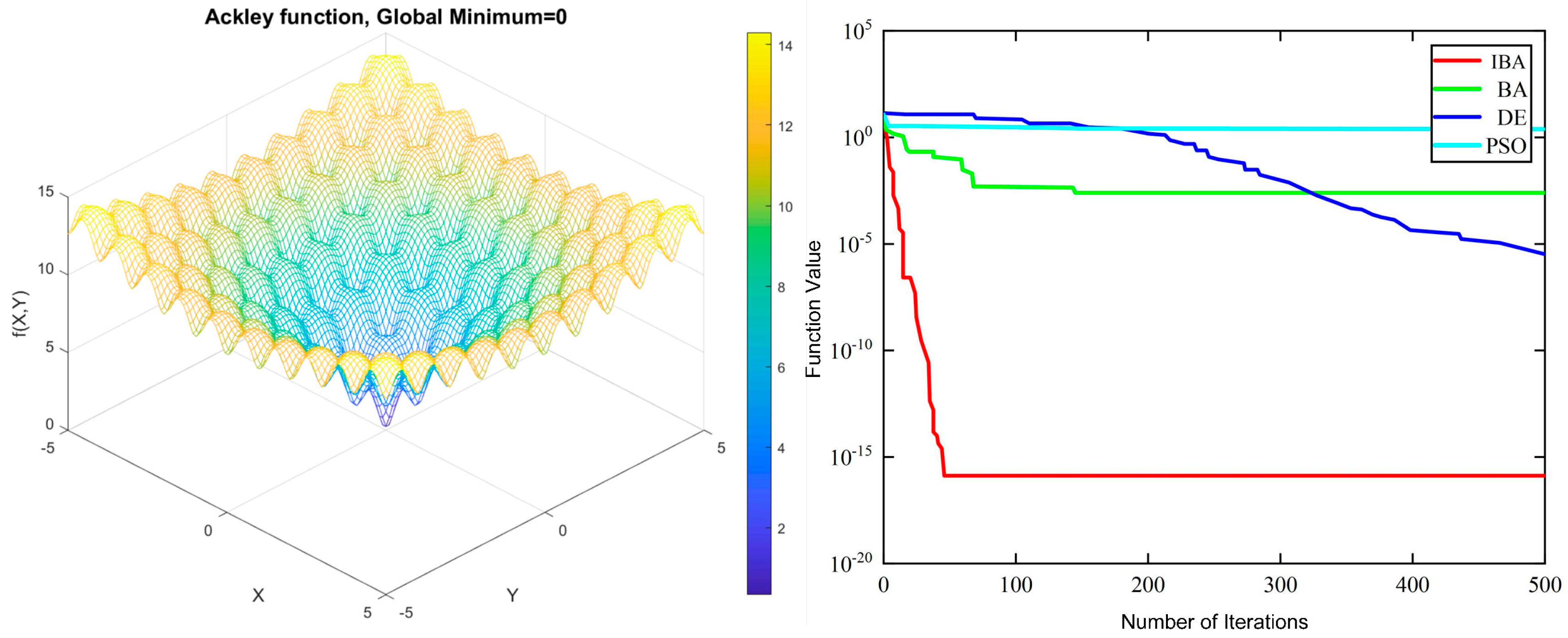
Figure 3 shows convergence curves of IBA, BA, DE, and PSO on the six benchmark functions. It can be observed that IBA converges faster and achieves lower fitness values than the other algorithms on all test functions. The comparative analysis of the experimental data in Table 3 and Figure 3 shows that the original BA outperforms PSO in both convergence efficiency and accuracy. However, in comparison with the DE algorithm, although the BA has a faster convergence rate, it often converges to local optimal solutions and terminates prematurely due to the lack of effective mechanisms for maintaining population diversity and mutation strategies. The optimized IBA exhibits obvious advantages in all performance indicators: the stability of its global optimal solution, worst solution and average solution is superior to that of the comparison algorithms, and the convergence accuracy is improved by several orders of magnitude. For nonlinear multimodal functions with multiple local extrema, the IBA can effectively avoid the local optimal trap and converge precisely to the global optimal solution of 0. In addition, the convergence speed of the IBA in the global search process is also significantly better than that of other algorithms. The experimental results demonstrate that the proposed IBA inherits the fast convergence characteristic of the original BA, and integrates the advantage of the DE algorithm in escaping from local optima. By optimizing the algorithm parameters based on the adaptive theory, the IBA significantly improves the convergence efficiency and accuracy, and exhibits superior optimization performance in solving global optimization problems.

Figure 3. Test functions and average convergence curves.

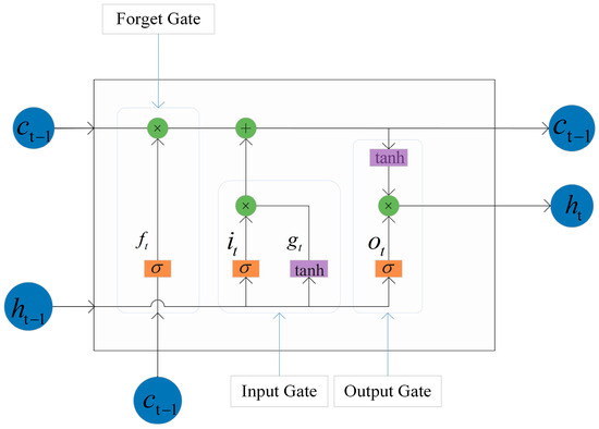
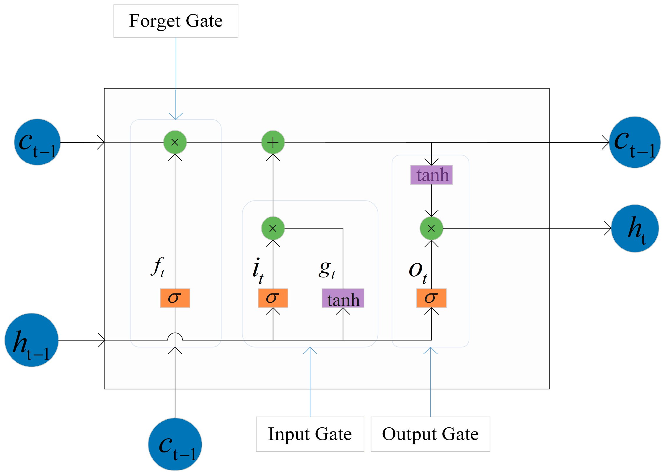
LSTM is an enhanced RNN model capable of overcoming the vanishing gradient problem, and its forecasting performance is directly influenced by the setting of key hyperparameters. The structure of the LSTM model is illustrated in Figure 4. This paper utilizes the Improved Bat Algorithm for optimization. The process formulates the LSTM hyperparameter search as a black-box optimization problem [30]. An individual bat’s position vector $x$ maps to a set of key LSTM hyperparameters, mainly including: the number of hidden layer neurons and the learning rate. The optimization objective is to minimize the LSTM model’s prediction error on the validation set. This paper uses Root Mean Square Error as the fitness function:

$$\mathrm{fitness}=\mathrm{RMSE}(y_i-\widehat{y_i})=\sqrt{{\displaystyle \frac{1}{n}}{\displaystyle \sum _{i=1}^N{(y_i-\widehat{y_i})}^2}}$$

(13)

Figure 4. The structure of the LSTM model.

The LSTM hyperparameters optimized by IBA include the number of hidden-layer neurons and the learning rate. Specifically, the number of hidden layer neurons is regarded as a model architecture hyperparameter, while the learning rate is regarded as a training hyperparameter. In this study, the position vector of each bat is defined as $X_i=[H_i,{\eta }_i]$, where $H_i$ denotes the number of hidden layer neurons and ${\eta }_i$ denotes the learning rate. The search ranges are set as follows: the number of hidden layer neurons is selected from [32, 64, 128, 256], and the learning rate is selected from [0.0005, 0.001, 0.005, 0.01]. The number of LSTM layers and the number of training epochs are kept fixed during the optimization process and are reported as model settings to ensure reproducibility. The optimization objective is to minimize the Root Mean Square Error (RMSE) on the validation set, as defined in Equation (13).

In the above formula, $y_i$ is the actual electricity price, and $\widehat{y_i}$ is the predicted electricity price. The IBA performs an iterative search in the hyperparameter space and finally outputs the global best position $x^{\ast }$, which represents the optimal LSTM hyperparameter combination found. This process improves the forecasting performance and robustness of the prediction model.

2.2.3. CEEMD-SE-IBA-LSTM Model

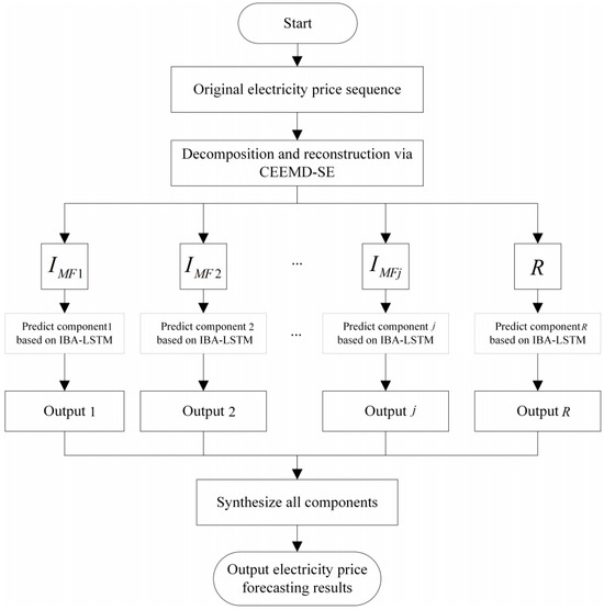
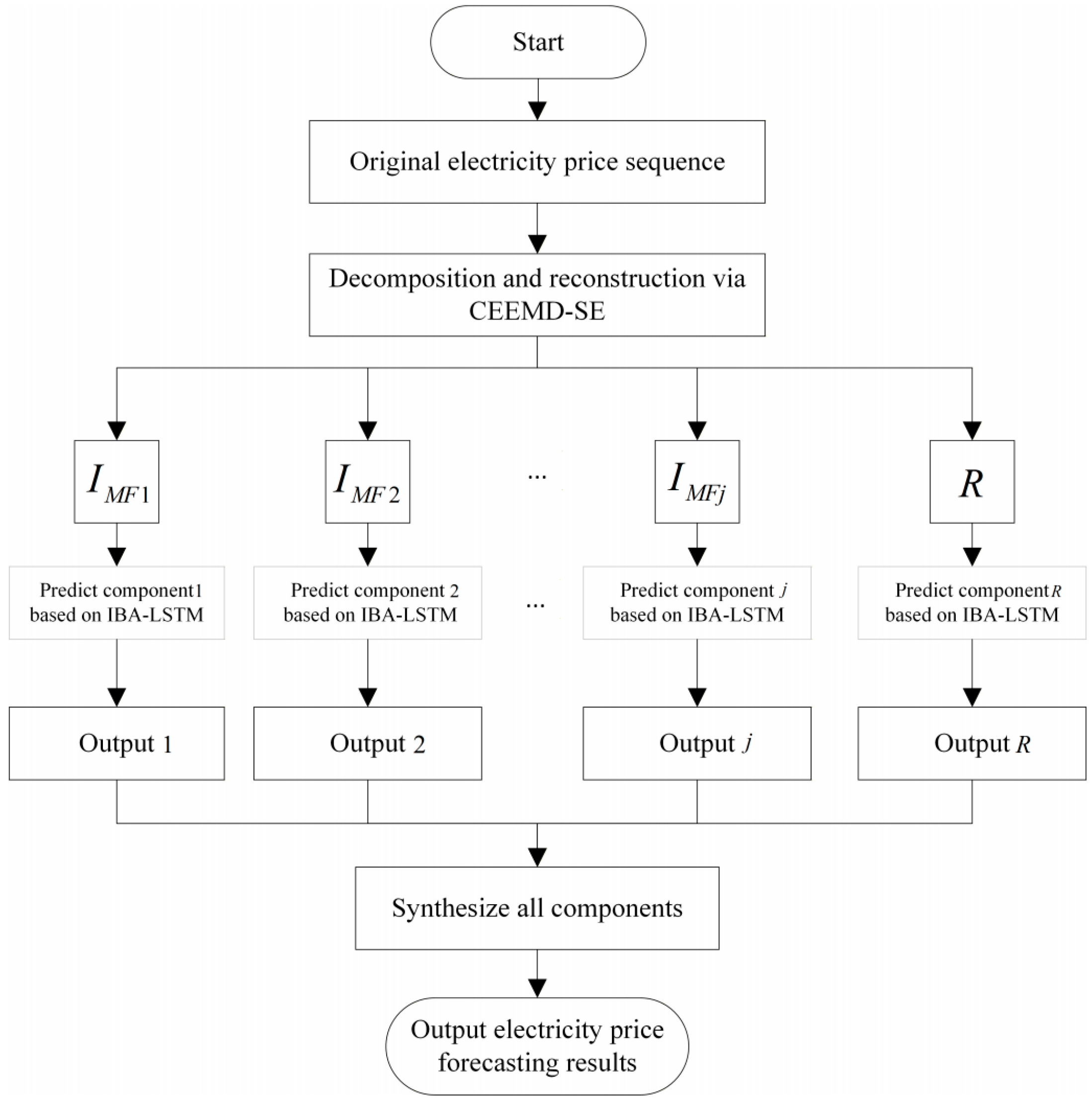
The CEEMD-SE-IBA-LSTM model proposed in this paper integrates the aforementioned modules to construct a complete day-ahead electricity price forecasting model. Its overall flowchart is shown in Figure 5. The execution steps of this model are as follows:

Figure 5. Electricity price forecasting model based on CEEMD-SE-IBA-LSTM.

The implementation process of this model mainly includes the following steps:

(1)

The CEEMD-SE algorithm is used to decompose and reconstruct the set of similar-day electricity price sequences, obtaining $j$ IMF modal components $\left\{\begin{array}{c}{I}_{MF1},I_{MF2},\dots ,I_{MFj}\end{array}\right\}$ and 1 residual term $R$.

(2)

Map each IMF modal component and residual term $R$ to the interval [−1, 1] using the max-min normalization method.

(3)

Utilize different components and combine with electricity price influencing factor data to train the corresponding IBA-LSTM regression models respectively.

(4)

Input the electricity price components and related influencing factor data of the day preceding the target forecast day into the trained IBA-LSTM models, and calculate the predicted value of each component respectively.

(5)

Denormalize the prediction results of the aforementioned components, and then synthesize them to output the final day-ahead electricity price prediction value.

3. Case Study and Model Verification

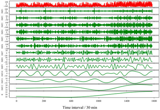
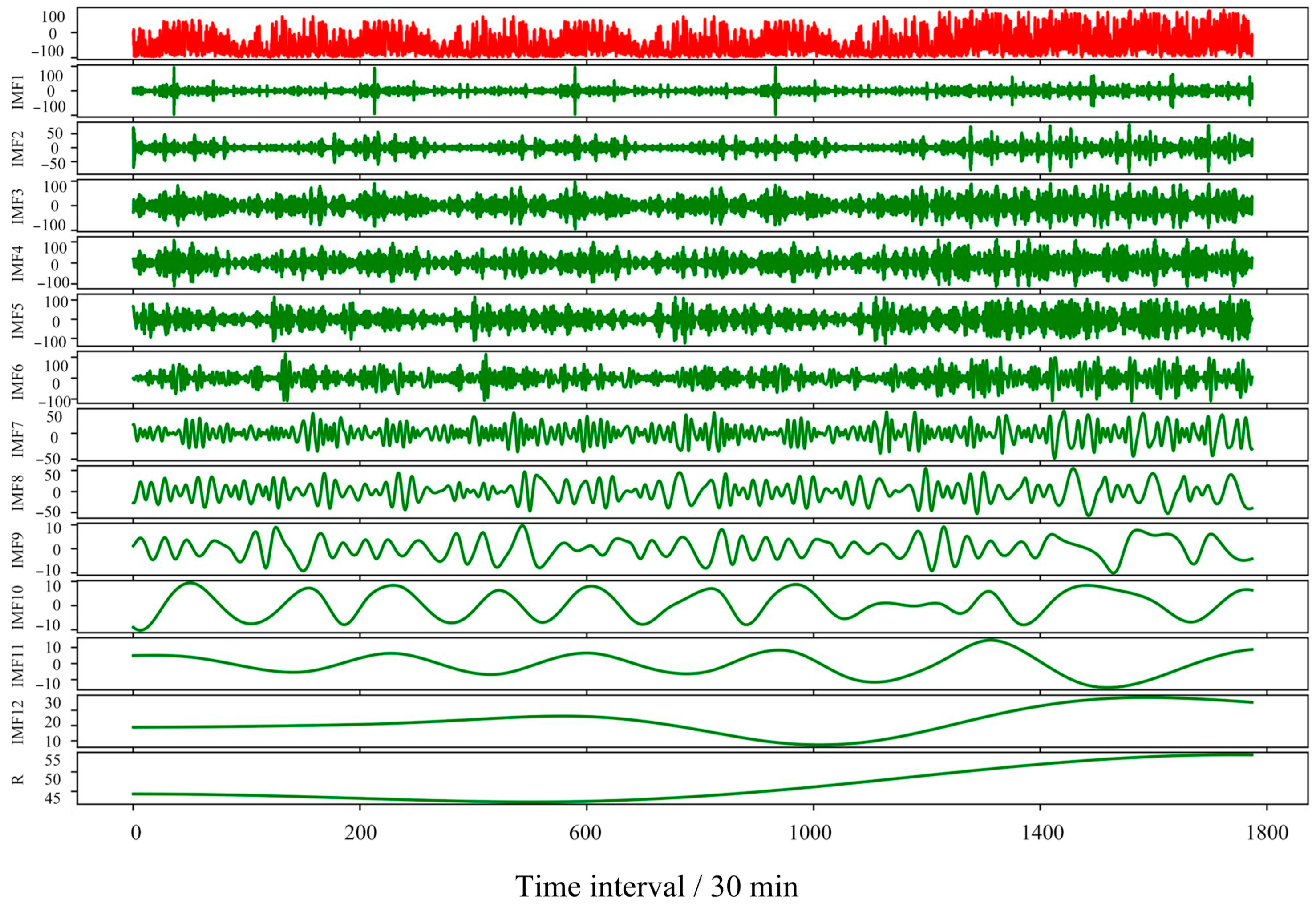
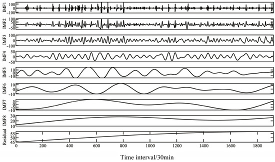
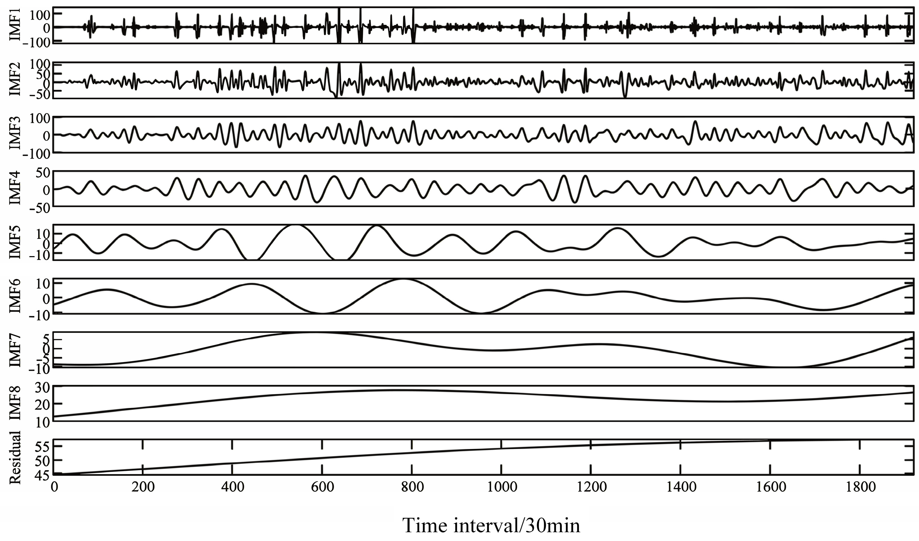
This study utilizes data from the US PJM electricity market. As the largest Regional Transmission Organization (RTO) in the US, covering 13 states and Washington D.C., serving over 65 million end-users, PJM is a globally mature market with high new energy penetration. The effectiveness and applicability of the proposed price forecasting model are verified through case study analysis. Multiple comparative forecasting models are constructed and tested. Their related error metrics are summarized and analyzed to evaluate the advantages of the proposed model from the perspective of prediction performance. Based on the RF-IAGIV model proposed earlier, the top 20 days ranked by similarity are selected from the historical price data to form the similar-day set. This set serves as the training dataset, with a sampling interval of 30 min, totaling 960 data points. Considering the significant volatility in price data, the original sequence is first decomposed using CEEMD, effectively smoothing data spikes. The output consists of 12 IMF components and 1 residual component, distributed from low to high frequency, all with relatively smooth variation trends, as shown in Figure 6.

Figure 6. CEEMD decomposition results of the electricity price series.

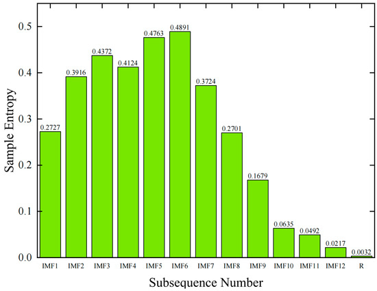
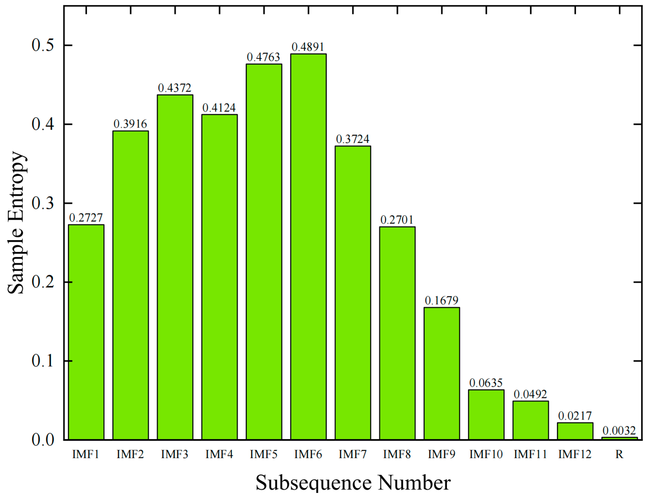
CEEMD decomposition yields 13 components. Directly modeling and predicting each subsequence with LSTM would increase computational load and overall model complexity. Therefore, SE theory is applied. With SE parameters m = 2 and r = 0.2, the complexity of each subsequence is calculated, as shown in Figure 7. Based on SE reconstruction theory, sub-sequences with sample entropy differences within 0.1 are classified and reconstructed together.

Figure 7. Sample entropy values of IMF components obtained by CEEMD.

To avoid an empirical selection of the reconstruction threshold, a sensitivity analysis was conducted for the sample-entropy-based reconstruction threshold $W$. The threshold $W$ represents the maximum allowable difference between the sample entropy values of two IMF components for reconstruction. A smaller $W$ leads to more reconstructed subsequences and preserves more local fluctuation information, but it increases the model complexity and training time. In contrast, a larger $W$ merges more components, reducing computational burden but potentially weakening the representation of high-frequency price fluctuations. Therefore, $W$ was tested within the range of 0.05–0.20 while keeping the CEEMD parameters, LSTM structure, and IBA optimization settings unchanged. The forecasting performance under different $W$ values is shown in Table 4.

Table 4. Sensitivity analysis of SE reconstruction threshold.

W	Number of Subsequences	MAPE (%)	RMSE ($/MWh)	MAE ($/MWh)
0.05	11	3.89	3.71	2.04
0.08	10	3.80	3.63	1.99
0.10	9	3.73	3.57	1.95
0.12	8	3.77	3.61	1.98
0.15	7	3.92	3.74	2.07
0.20	6	4.16	3.98	2.23

As shown in Table 4, when $W=0.10$, the proposed model achieves the lowest MAPE, RMSE, and MAE among the tested thresholds. When $W$ is smaller than 0.10, excessive component separation increases model complexity and may introduce redundant high-frequency information. When $W$ is larger than 0.10, excessive component merging weakens the ability of the model to capture local price fluctuations. Therefore, $W=0.10$ was selected as the reconstruction threshold in this study. This result also confirms that the selected threshold is not arbitrary but determined based on forecasting performance and model complexity.

As seen in Figure 7, the sample entropy values of subsequences IMF2-IMF6 are close. These five subsequences are grouped into one category. After integration and reconstruction, they form a new subsequence input for LSTM training and prediction. Classifying all subsequences results in 9 groups. The result after classification and reconstruction is shown in Figure 8.

Figure 8. Reconstructed electricity price components based on CEEMD-SE.

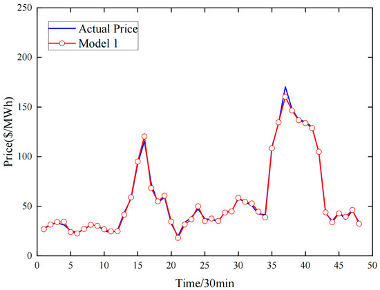
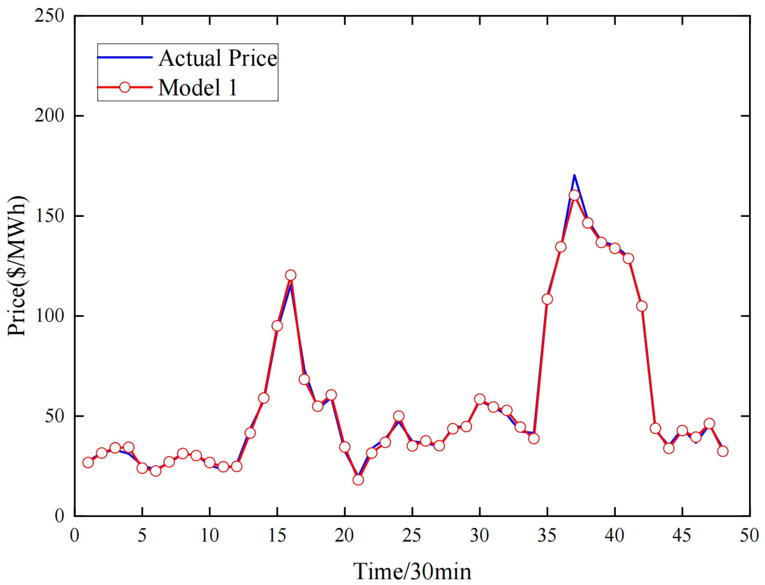
The prediction results of each component are recombined to obtain the day-ahead price forecast for the target day. A comparison with the actual price curve is shown in Figure 9. The model achieves high prediction accuracy for most time points, demonstrating strong generalization performance, although there is room for improvement in forecasting peak prices. To further analyze prediction errors, the absolute relative error of the predicted values was calculated, as shown in Table 5. Among the 48 forecasted time points, the absolute relative error ranges from 0.41% to 12.35%, with an average of 3.73%. Error distribution analysis indicates that the model provides more accurate predictions during stable price periods, while errors increase somewhat during peak and valley price periods. Overall, the model exhibits good forecasting performance.

Figure 9. Model CEEMD-SE-IBA-LSTM predictive value analysis chart.

Table 5. Electricity price forecast value and error table.

Time	Actual Price/($/MWh)	Predicted Value/($/MWh)	Absolute Relative Error
0:30	27.47	26.76	2.56%
1:00	31.69	31.52	0.54%
1:30	33.10	34.12	3.09%
2:00	31.23	34.39	10.13%
2:30	25.35	23.94	5.56%
3:00	23.24	22.54	3.03%
3:30	26.76	27.11	1.31%
4:00	30.99	31.28	0.95%
4:30	30.53	30.28	0.81%
5:00	25.35	26.76	5.54%
5:30	23.24	24.65	6.06%
6:00	26.06	24.85	4.62%
6:30	43.66	41.55	4.84%
7:00	57.75	59.01	2.19%
7:30	92.96	95.07	2.27%
8:00	115.50	120.42	4.27%
8:30	73.24	68.31	6.73%
9:00	53.52	54.93	2.63%
9:30	59.15	60.56	2.38%
10:00	32.39	34.51	6.52%
10:30	19.72	18.08	8.29%
11:00	33.80	31.49	6.84%
11:30	38.73	36.87	4.80%
12:00	47.18	49.96	5.89%
12:30	37.32	35.07	6.03%
13:00	36.62	37.56	2.57%
13:30	34.62	35.16	1.55%
14:00	44.37	43.66	1.59%
14:30	45.07	44.75	0.70%
15:00	57.75	58.45	1.22%
15:30	54.22	54.50	0.51%
16:00	50.70	52.82	4.17%
16:30	42.25	44.48	5.27%
17:00	41.55	38.73	6.78%
17:30	109.86	108.45	1.28%
18:00	133.80	134.51	0.53%
18:30	170.42	160.38	12.35%
19:00	147.89	146.48	0.95%
19:30	137.33	136.76	0.41%
20:00	135.21	133.81	1.04%
20:30	129.58	128.75	0.64%
21:00	104.23	104.93	0.68%
21:30	42.96	43.85	2.08%
22:00	35.21	33.84	3.86%
22:30	43.66	42.77	2.03%
23:00	36.62	39.43	7.69%
23:30	45.66	41.56	9.01%
0:00	33.80	32.39	4.17%

The residuals are relatively small during stable price periods, indicating that the proposed CEEMD-SE-IBA-LSTM model can effectively capture the regular fluctuation trend of day-ahead electricity prices. However, larger prediction deviations mainly occur during rapid price changes and peak-price periods, such as the largest relative error around 18:30, suggesting that sudden price spikes remain more difficult to predict.

To further evaluate the performance of the proposed CEEMD-SE-IBA-LSTM model and verify the effectiveness of its data processing methods and optimization algorithms, this study constructs six comparison models and conducts a comparative analysis with the proposed model to explore performance differences. The construction methods of each model are shown in Table 6.

Table 6. Different prediction methods.

Model Category	Method	Training Time
Proposed Model 1	Similar-day selection + CEEMD-SE-IBA-LSTM	40.0 min
Ablation Model 2	Similar-day selection + IBA-LSTM	28.0 min
Ablation Model 3	Similar-day selection + LSTM	4.5 min
Comparison Model 4	Similar-day selection + ELM	0.8 min
Comparison Model 5	Similar-day selection + BP	3.2 min
Comparison Model 6	Similar-day selection + CNN	6.5 min
Ablation Model 7	CEEMD-SE-IBA-LSTM	42.0 min

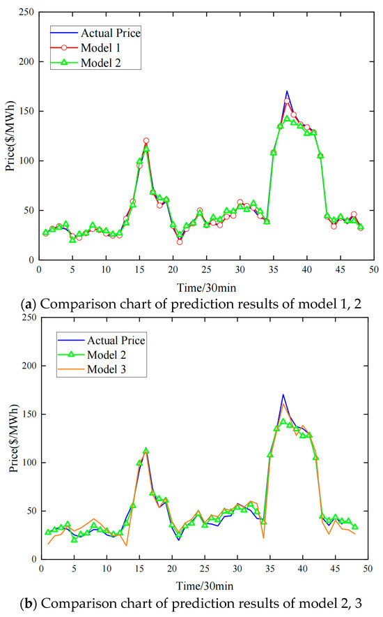
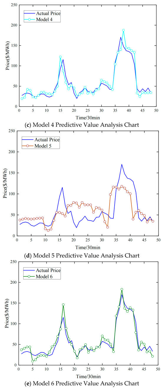
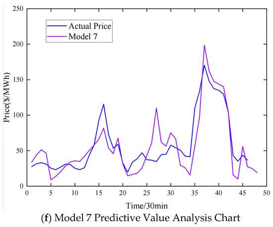
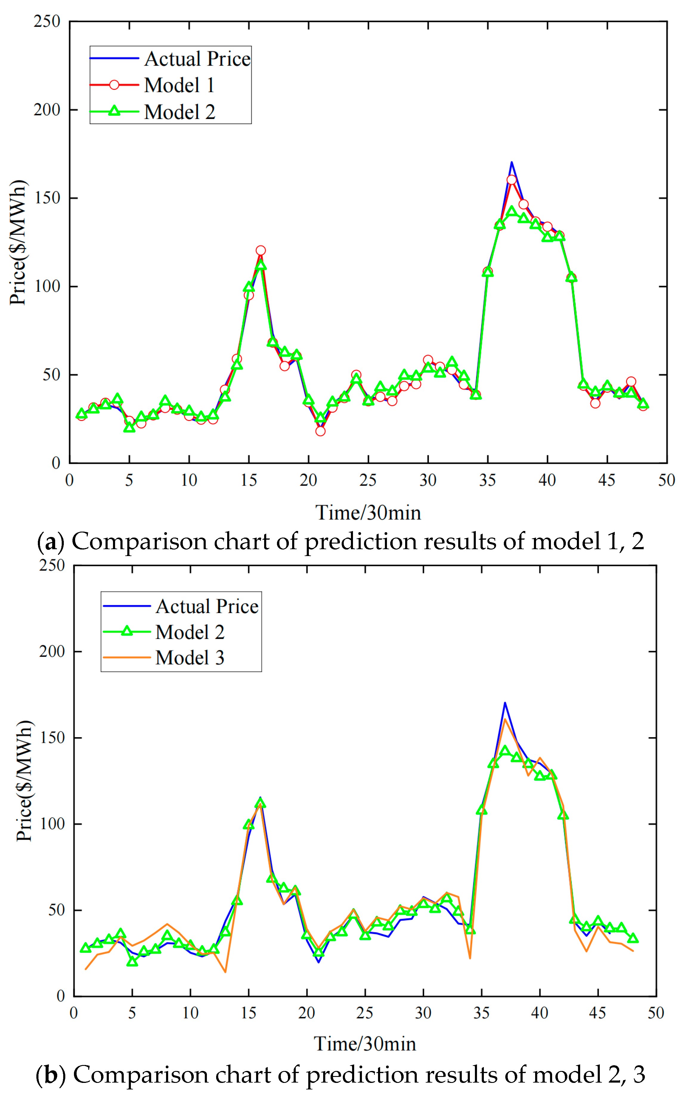
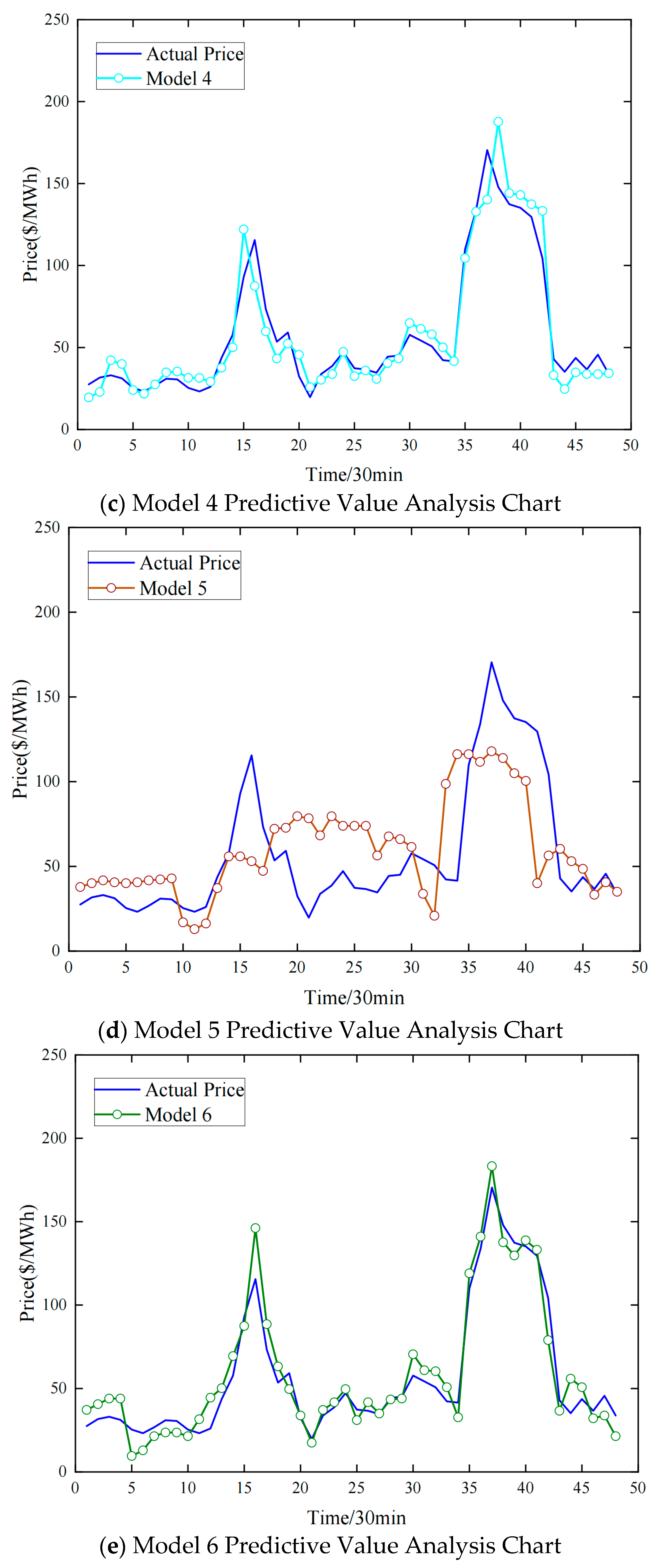
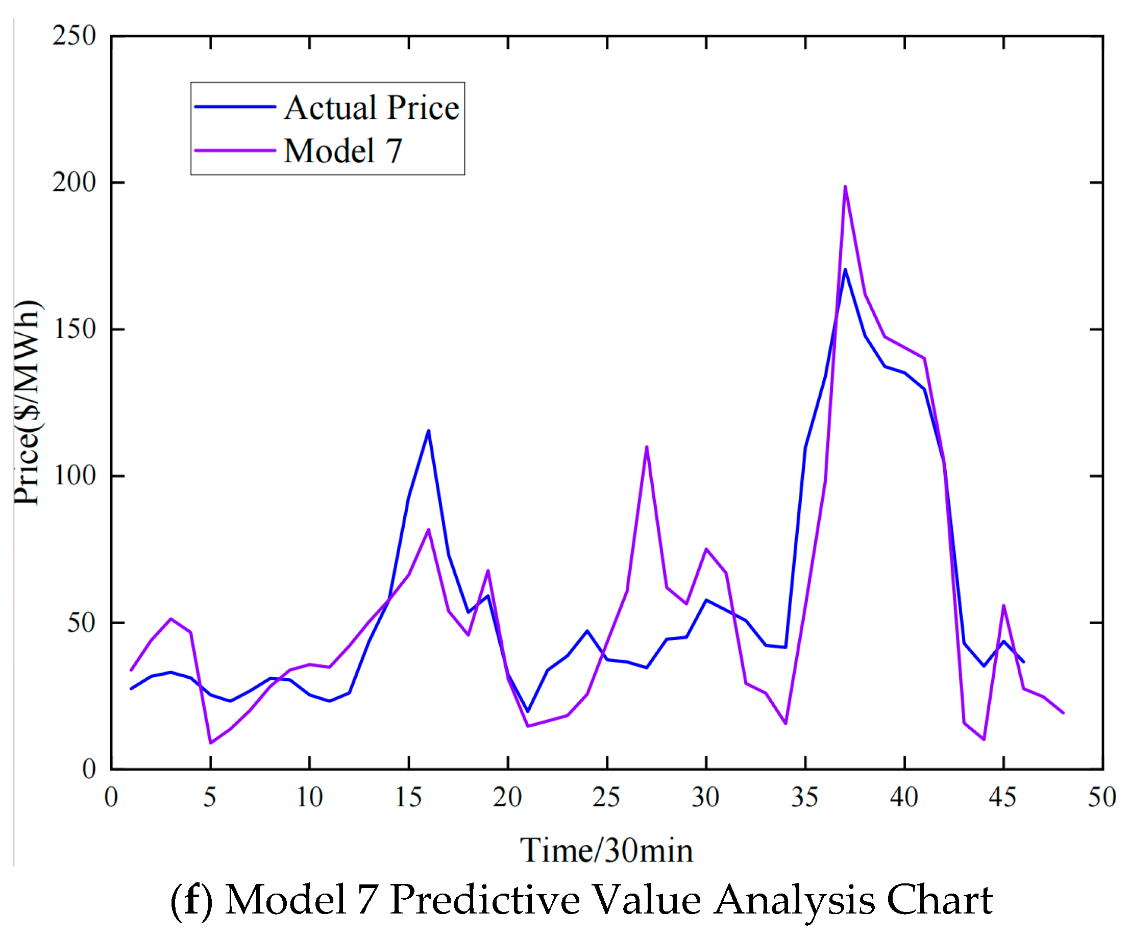
For ease of discussion below, the model proposed in this paper is defined as Model 1. Ablation Model 2 does not use CEEMD-SE decomposition/reconstruction on the original price, directly applying the IBA-LSTM model. Ablation Model 3 uses LSTM without IBA optimization. Comparison Model 4 uses Extreme Learning Machine (ELM). Comparison Model 5 uses a Backpropagation Neural Network (BP). Comparison Model 6 uses a Convolutional Neural Network (CNN). Ablation Model 7 uses CEEMD-SE-IBA-LSTM but without similar-day screening. The comparison results are shown in Figure 10.

Figure 10. Comparison chart of prediction results.

It should be noted that the comparison models serve different roles in the experimental analysis. The contribution of IBA-based hyperparameter optimization is mainly evaluated by comparing Ablation Model 2 and Ablation Model 3, both of which use the same similar-day dataset and LSTM structure, with the only difference being whether IBA is used for hyperparameter optimization. Therefore, the comparison between Ablation Model 2 and Ablation Model 3 directly reflects the effect of IBA optimization. In contrast, ELM, BP, and CNN are introduced as representative baseline forecasting models to evaluate the overall forecasting performance of the proposed hybrid framework. To reduce the influence of unfair parameter settings, all comparison models were trained and tested using the same dataset, and the main parameters of ELM, BP, and CNN were set according to their validation-set performance and commonly used model configurations.

To further evaluate the computational applicability of the proposed model, the training time of each compared model was recorded under the same hardware and software environment, as shown in Table 6. Although the proposed CEEMD-SE-IBA-LSTM model requires a longer training time due to CEEMD-SE decomposition and population-based hyperparameter optimization, its training time is approximately 40 min, and the optimization process is performed offline. After training, the online prediction time is short enough to satisfy the requirements of day-ahead electricity price forecasting.

Figure 10 shows that the proposed CEEMD-SE-IBA-LSTM model (Model 1) performs best in PJM price forecasting. After preprocessing, parameter optimization, and similar-day selection, its predictions closely follow the actual price curve. In contrast, comparison models (ELM, BP, CNN) and ablation models (without optimization or preprocessing) show significant errors during price fluctuations. This fully demonstrates the proposed model’s advantage in capturing complex price characteristics and improving prediction accuracy.

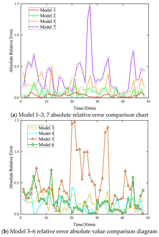
To comprehensively compare the forecasting performance of Model 1 with the other six models, the absolute relative error for each model is calculated, as shown in Figure 11.

Figure 11. Comparison chart of absolute values of relative errors of each model.

Figure 11a, through the comparison of absolute relative error, intuitively presents the differences in prediction accuracy among the models. The error curve for Model 1 consistently resides in the lowest interval. For 98% of the forecast points, the error is below 5%. During peak price hours, errors are only 2.1% and 1.8%, indicating the highest alignment with actual prices. The error curve for Ablation Model 2 (without CEEMD-SE preprocessing) shows significantly greater fluctuation, with peak-hour errors reaching 8.3%. The error curve for Ablation Model 3 (without IBA optimization) shows errors of 6.7% and 7.2% during mid-low price periods (e.g., hours 15, 33). For Ablation Model 7 (without similar-day screening), the error curve is generally elevated, with an average error of 12.4% and a peak error of 21.7% at points of sudden price change.

Figure 11b focuses on the error performance of comparison models like ELM, BP, and CNN. The BP model has the worst accuracy, with a mean absolute relative error of 18.9% and a maximum error of 35.2%. The mean errors for ELM and CNN models are 10.5% and 9.8%, respectively, but still exceed 15% during price fluctuations. Ablation Model 3 (LSTM-based) has a mean error of 7.1%. This further confirms that similar-day selection enhances data relevance, CEEMD-SE preprocessing improves sequence stationarity, and IBA parameter optimization accelerates LSTM convergence. The combination of these three plays a key role in reducing prediction errors. A comparison of error metrics is shown in Table 7.

Table 7. Comparison of error indicators.

Error Metric	Model 1	Model 2	Model 3	Model 4	Model 5	Model 6	Model 7
MAE ($/MWh)	1.95	3.67	6.93	8.39	25.03	8.79	16.01
MAPE (%)	3.73	7.34	15.37	15.48	53.26	19.87	36.06
RMSE ($/MWh)	3.57	5.50	7.81	12.02	31.99	10.71	19.03

From the error indicator analysis, the proposed model (Model 1) demonstrates the most outstanding performance, with an MAPE of 3.73%, MAE of 1.95 $/MWh, and RMSE of 3.57 $/MWh, which are optimal among all compared models.

The high error of Ablation Model 7 further indicates that similar-day selection is a key step in the proposed framework. Without RF-IAGIV-based screening, the training samples may contain historical days with weak similarity to the target forecasting day, thereby introducing irrelevant price patterns and significantly reducing forecasting accuracy. Meanwhile, to avoid overfitting to an overly narrow historical period, the top 20 similar days are selected to balance sample similarity and diversity.

4. Discussion

It should be noted that the current study does not include a direct ablation experiment comparing the model performance with and without the new energy penetration indicators, namely WD, SD, RW, and RS. Although the correlation analysis in Table 1 indicates that these indicators are closely related to electricity price fluctuations, their individual and combined contributions to forecasting accuracy have not been quantitatively isolated in this work. This is a limitation of the present study. In future work, systematic ablation experiments will be conducted to compare forecasting performance before and after introducing these penetration indicators, so as to further quantify their contribution to model accuracy and generalization ability.

In addition, although the PJM dataset used in this study covers the year 2023 and contains different seasonal conditions, the current experimental validation is still mainly based on the selected forecasting case and the corresponding similar-day training set. Since electricity price patterns may vary significantly across seasons and years due to changes in load demand, renewable generation, fuel prices, and market operation conditions, the seasonal and multi-year generalization ability of the proposed model has not been fully verified in this work. This is another limitation of the present study. In future work, representative forecasting periods from different seasons, such as winter and summer, as well as multi-year PJM datasets and other electricity markets, will be further introduced to evaluate the long-term robustness and generalization ability of the proposed model.

5. Conclusions

This paper addresses the challenge of day-ahead electricity price forecasting in power markets with high-penetration renewable energy integration. A combined forecasting model named CEEMD-SE-IBA-LSTM based on multi-information fusion is proposed. The RF-IAGIV method selects similar days, using RF to quantify the importance of 13 factors and assign weights, combined with IAGIV to select the top 20 similar days. The price series is decomposed and reconstructed by CEEMD-SE into 9 stationary components. IBA is used to optimize LSTM parameters. Using 2023 data from the US PJM market as a sample, comparisons are made with ablation and traditional models. The simulation yields the following conclusions:

(1)

This study emphasizes the impact of renewable energy generation on day-ahead electricity prices in power markets. The incorporation of renewable energy penetration indicators provides additional information for characterizing the influence of wind and photovoltaic generation on day-ahead electricity prices. However, the independent contribution of these indicators to forecasting accuracy still requires further verification through systematic ablation experiments.

(2)

A similar-day selection method based on RF-IAGIV is proposed. This combined model simplifies the forecasting process, improves efficiency, and lays a solid foundation for subsequent day-ahead price prediction.

(3)

A data preprocessing technique based on CEEMD-SE is proposed. Decomposing and reconstructing the original price time series yields multiple component sequences with smoother fluctuations. Experimental results show that preprocessing data before forecasting simplifies the prediction difficulty and significantly enhances accuracy.

(4)

An electricity price forecasting model based on IBA-LSTM is proposed. Case study analysis results indicate that the proposed combined model possesses significant advantages in price forecasting accuracy.

In summary, the electricity price forecasting model proposed in this paper exhibits outstanding performance, considerable prediction accuracy, and good generalizability.

References

- Raineri, R. Power shift: Decarbonization and the new dynamics of energy markets. Energies 2025, 18, 752. [Google Scholar] [CrossRef]
- Özcan, A.V.; Erel-Özçevik, M.; Karaman, B.; Baştürk, İ.; Zeydan, E.; Taşkın, S.; Çetinkaya, Ü. Forecasting day-ahead electricity prices for the electricity market with dynamic time period. Energy 2025, 338, 138766. [Google Scholar] [CrossRef]
- Meng, A.; Zhu, J.; Yan, B.; Yin, H. Day-ahead electricity price prediction in multi-price zones based on multi-view fusion spatio-temporal graph neural network. Appl. Energy 2024, 369, 123553. [Google Scholar] [CrossRef]
- Pavlík, M.; Bereš, M. Effects of electricity price volatility, energy mix and training interval on prediction accuracy: An investigation of adaptive and static regression models for Germany, France and the Czech Republic. Energies 2025, 18, 3893. [Google Scholar] [CrossRef]
- Lin, O.Z.; Koutroulis, E.; Štěpanec, L.; Aye, H.Y.; Juchelkova, D. Decentralized solar PV systems for energy resilience: Lessons from Myanmar’s post-2021 political turmoil using field test data. Renew. Energy 2026, 267, 125793. [Google Scholar] [CrossRef]
- Xiong, X.; Qing, G. A hybrid day-ahead electricity price forecasting framework based on time series. Energy 2023, 264, 126099. [Google Scholar] [CrossRef]
- Ghelasi, P.; Ziel, F. From day-ahead to mid and long-term horizons with econometric electricity price forecasting models. Renew. Sustain. Energy Rev. 2025, 217, 115684. [Google Scholar] [CrossRef]
- Zhang, Z.; Hua, H.; Chen, X.; Shao, J.; Zheng, J.; Wang, B.; Gan, L.; Yu, K. Spot market electricity price forecast via the combination of transformer and Ornstein-Uhlenbeck process. In Proceedings of the 2025 21st International Conference on the European Energy Market (EEM); IEEE: Piscataway, NJ, USA, 2025; pp. 1–6. [Google Scholar]
- Jan, F.; Iftikhar, H.; Tahir, M.; Khan, M. Forecasting day-ahead electric power prices with functional data analysis. Front. Energy Res. 2025, 13, 1477248. [Google Scholar] [CrossRef]
- Kontogiannis, D.; Bargiotas, D.; Daskalopulu, A.; Arvanitidis, A.I.; Tsoukalas, L.H. Error compensation enhanced day-ahead electricity price forecasting. Energies 2022, 15, 1466. [Google Scholar] [CrossRef]
- Li, C.; Liu, Z.; Zhang, G.; Sun, Y.; Qiu, S.; Song, S.; Wang, D. Day-ahead electricity price forecasting for sustainable electricity markets: A multi-objective optimization approach combining improved NSGA-II and RBF neural networks. Sustainability 2025, 17, 4551. [Google Scholar] [CrossRef]
- Luo, H.; Shao, Y. Advanced optimal system for electricity price forecasting based on hybrid techniques. Energies 2024, 17, 4833. [Google Scholar] [CrossRef]
- Aksu, İ.Ö.; Ghaemi, S.; Anvari-Moghaddam, A. A two-stage deep learning approach for accurate day-ahead electricity price forecasting. Eng. Appl. Artif. Intell. 2026, 163, 112721. [Google Scholar] [CrossRef]
- He, M.; Jiang, W.; Gu, W. TriChronoNet: Advancing electricity price prediction with multi-module fusion. Appl. Energy 2024, 371, 123626. [Google Scholar] [CrossRef]
- Ghimire, S.; Nguyen-Huy, T.; Deo, R.C.; Casillas-Pérez, D.; Ahmed, A.M.; Salcedo-Sanz, S. Novel deep hybrid model for electricity price prediction based on dual decomposition. Appl. Energy 2025, 395, 126197. [Google Scholar] [CrossRef]
- Laitsos, V.; Vontzos, G.; Bargiotas, D.; Daskalopulu, A.; Tsoukalas, L.H. Data-driven techniques for short-term electricity price forecasting through novel deep learning approaches with attention mechanisms. Energies 2024, 17, 1625. [Google Scholar] [CrossRef]
- Liu, D.; Lei, Z.; Sun, K. Short-term electricity price forecasting based on wavelet packet decomposition and long short-term memory network. Smart Power 2020, 48, 77–83. [Google Scholar]
- Rawal, K.; Ahmad, A. Mining latent patterns with multi-scale decomposition for electricity demand and price forecasting using modified deep graph convolutional neural networks. Sustain. Energy Grids Netw. 2024, 39, 101436. [Google Scholar] [CrossRef]
- Gomez, W.; Wang, F.K.; Lo, S.C. A hybrid approach based machine learning models in electricity markets. Energy 2024, 289, 129988. [Google Scholar] [CrossRef]
- Li, X.; He, T.; Zhu, W.; Xu, Q. HE-DTimeXer: A short-term electricity price prediction model with exogenous variables. Electr. Power Syst. Res. 2026, 253, 112540. [Google Scholar] [CrossRef]
- Tang, F.; Dou, Z.; Cao, Y.; Zhang, C. An integrated energy system flexible resource feature extraction and identification method for electricity spot market. Energy Inform. 2025, 8, 122. [Google Scholar] [CrossRef]
- Ai, Y.; Jia, Y.B.; Han, X.Q. Day-ahead electricity price forecasting method based on similar day screening and combined deep learning model. Power Syst. Technol. 2025, 49, 242–251. [Google Scholar]
- Sun, Y.; Zhao, X.; Dai, H.; Wang, F.; Feng, G. A medium-term daily electricity consumption rolling multi-step forecasting method considering meteorologically similar days. In Proceedings of the 2025 IEEE Industry Applications Society Annual Meeting (IAS); IEEE: Piscataway, NJ, USA, 2025; pp. 1–8. [Google Scholar]
- Planert, D.E.; Bender, T.; Rippstein, F.; Klaiber, S. Feature selection for electricity market data through feature extraction. In 2025 21st International Conference on the European Energy Market (EEM); IEEE: Piscataway, NJ, USA, 2025; pp. 1–9. [Google Scholar]
- Zhou, T.H.; Xun, X.; Wang, L.; Hu, G.; Ding, W.; Kou, L. Self-adaptive clustering model based on variable time-series similarity measure analysis for V2G electricity price prediction. Appl. Sci. 2025, 15, 2069. [Google Scholar] [CrossRef]
- Li, M.; Wang, X. Short-term electricity price forecasting via CPO-enhanced dual decomposition and NRBO-optimized deep learning. Digit. Signal Process. 2025, 168, 105520. [Google Scholar]
- Richman, J.S.; Moorman, J.R. Physiological time-series analysis using approximate entropy and sample entropy. Am. J. Physiol.-Heart Circ. Physiol. 2000, 278, H2039–H2049. [Google Scholar] [CrossRef] [PubMed]
- Pebrianti, D.; Ann, N.Q.; Bayuaji, L.; Abdullah, N.R.H.; Zain, Z.M.; Riyanto, I. Extended bat algorithm (EBA) as an improved searching optimization algorithm. In Proceedings of the 10th National Technical Seminar on Underwater System Technology 2018: NUSYS’18; Springer: Singapore, 2019; pp. 229–237. [Google Scholar]
- Pang, A.; Liang, H.; Lin, C.; Yao, L. A surrogate-assisted adaptive bat algorithm for large-scale economic dispatch. Energies 2023, 16, 1011. [Google Scholar] [CrossRef]
- Ahmadvand, F.; Imani, M.H.; Andani, H.T.; Andani, M.T. Optimizing the LSTM model for electricity price forecasting using the MSADBO algorithm. In Proceedings of the 2025 IEEE Texas Power Energy Conference (TPEC); IEEE: Piscataway, NJ, USA, 2025; pp. 1–6. [Google Scholar]
Disclaimer/Publisher’s Note: The statements, opinions and data contained in all publications are solely those of the individual author(s) and contributor(s) and not of MDPI and/or the editor(s). MDPI and/or the editor(s) disclaim responsibility for any injury to people or property resulting from any ideas, methods, instructions or products referred to in the content. |
© 2026 by the authors. Licensee MDPI, Basel, Switzerland. This article is an open access article distributed under the terms and conditions of the Creative Commons Attribution (CC BY) license.