


Abstract
Large-scale integration of renewable energy sources and power-electronic equipment introduces substantial background harmonics into the grid and, at the same time, gives rise to weak-grid operating conditions with a low short-circuit ratio, thereby degrading the power quality and stability of grid-connected converters. This paper investigates a three-phase LCL-type grid-connected converter and establishes a dq-domain admittance model that incorporates the DC-voltage outer loop, the phase-locked loop (PLL), and grid-voltage feedforward. On the basis of admittance-reshaping theory, a method is proposed to suppress the influence of background harmonics and enhance system stability. First, the frequency coupling caused by the structural asymmetry of the PLL and the voltage outer loop is decoupled to reduce the harmonic components in the grid current. Then, based on the decoupled model, the grid-voltage feedforward path is compensated to eliminate the negative-damping region in the converter output admittance and thus improve system stability under weak-grid conditions. Finally, simulation and experimental results verify the effectiveness of the proposed method.
1. Introduction
With the continued implementation of China’s carbon peaking and carbon neutrality strategy, renewable clean energy sources such as photovoltaic and wind power have been vigorously developed [1,2]. As the interface between the grid and renewable-energy generation systems, a grid-connected converter is directly related to power quality, system stability, and overall grid security. However, the ever-increasing penetration of renewable sources and power-electronic equipment has introduced a large amount of background harmonics into the grid and reduced the effective short-circuit ratio, thereby producing weak-grid conditions characterized by large and time-varying equivalent impedances [3]. Such conditions degrade the power quality of grid-connected systems and frequently lead to stability problems. In the Guyuan wind-farm area of Hebei, 6–8 Hz oscillations caused severe distortion of grid voltage and current [4]. In the Qinghai Power Grid, second-harmonic components generated during the energization of an unloaded transformer caused a bipolar blocking accident in the Qinghai–Tibet HVDC link [5,6]. In Hami, Xinjiang, inter-harmonics with time-varying frequencies in direct-drive wind farms repeatedly caused local voltage fluctuation and flicker [7,8]. Since 2020, high-frequency resonance has occurred frequently at the Kangbanuoer converter station of the Zhangbei DC project, threatening stable system operation [9]. Therefore, it is of great engineering significance to improve the power quality and stability of grid-connected converters under weak-grid conditions and background harmonic disturbances.
A large number of existing studies focus on suppressing the effect of background harmonics on grid-connected converters through admittance reshaping. Owing to the asymmetric control structure of a three-phase grid-connected converter, frequency coupling arises. When background harmonics are present, the resulting image harmonics severely deteriorate power quality [10]. To eliminate frequency coupling, references [11,12] designed a structurally symmetric PLL that reshapes the original double-input double-output impedance model into a single-input single-output one, thereby eliminating frequency coupling; however, the asymmetry of the outer-loop control structure was not considered. Reference [13] considered the asymmetric structures of the power outer loop and the PLL to decouple frequency coupling, but its suppression effect on the coupling introduced by the power outer loop was unsatisfactory. In addition, reducing the admittance magnitude via admittance reshaping can also effectively mitigate the influence of background harmonics. References [14,15] achieved this by proportional grid-voltage feedforward or full grid-voltage feedforward. However, proportional feedforward suppresses low-frequency harmonics while amplifying high-frequency ones and therefore cannot realize broadband harmonic suppression. Full feedforward, when control delay is considered, tends to impair system robustness and reduce stability [16]. Reference [17] proposed an automatically adjustable virtual-impedance control strategy to improve grid-current power quality, but it is applicable only to low-order steady-state harmonics and entails excessive computational burden. References [18,19,20] adopted different perspectives: in the stationary frame, PR plus multi-resonant harmonic compensators were employed; in the synchronous rotating frame, PI plus multi-resonant harmonic compensators were used. These methods suppress the influence of specific background harmonics by increasing the loop gain at the corresponding harmonic frequencies. Although target harmonics can be selectively eliminated, such methods are highly sensitive to parameter drift, and multi-resonant controllers readily destabilize the system [21].
For the stability problem under weak-grid conditions, researchers have analyzed and improved grid-connected systems from the impedance perspective. Existing studies mainly fall into two categories. One category focuses on control parameter optimization. For a grid-connected inverter system under weak-grid conditions, reference [22] proposed a general PLL parameter-optimization design method with good applicability based on the small-signal impedance model and the constraint on PLL harmonic-disturbance rejection capability. Reference [23] improved system stability by reducing the grid-voltage feedforward gain. However, parameter tuning cannot adapt to large variations in grid impedance, and the dynamic performance of the system may also be affected. The other category optimizes the control structure of the grid-connected system. Based on passivity theory, reference [24] designed a phase-margin compensation method over divided frequency bands, thereby enhancing the stability of grid-connected converters under weak-grid conditions, but the adverse influence of frequency-coupling effects was ignored. Reference [25] introduced an oscillation-suppression controller into the control structure to block signals at the oscillatory frequency and improve the converter phase margin within the target frequency band, but this method cannot enhance stability over a wide frequency range.
In summary, the existing frequency decoupling methods exhibit unsatisfactory performance. Meanwhile, conventional admittance-reshaping strategies fail to suppress wideband background harmonics commonly present in power grids and tend to degrade the stability of grid-connected converters. Moreover, parameter optimization and admittance-reshaping approaches developed for stability enhancement under weak grid conditions cannot simultaneously improve power quality. Consequently, most existing control schemes for grid-connected converters under weak grids only address either background harmonic disturbances or system stability, and are incapable of achieving harmonic suppression and wide-range weak grid stability concurrently. Taking the LCL-type grid-connected converter as the research object, this paper proposes a control optimization method based on admittance reshaping to tackle the power quality and stability issues caused by background harmonics and weak grid conditions. The presented method realizes the coordinated implementation of frequency coupling decoupling and passive admittance reshaping within a unified model, which simultaneously mitigates weak grid oscillations and background harmonic distortion and overcomes the limitations of existing methods. Firstly, the admittance model of the grid-connected converter is established in the dq frame by fully considering the outer DC voltage loop, phase-locked loop (PLL) and grid-voltage feedforward. Secondly, decoupling compensation is adopted to eliminate frequency coupling induced by the structural asymmetry of the PLL and voltage outer loop, which suppresses the image harmonic currents generated when background harmonics act on the converter and improves grid power quality. On the basis of the decoupling scheme, the grid-voltage feedforward path is further compensated to eliminate the negative-damping region of the converter output admittance. This scheme attenuates the adverse impacts of background harmonics and effectively enhances the stability of the grid-connected system under weak grid conditions.
2. Admittance Model of the Three-Phase LCL-Type Grid-Connected Converter
2.1. System Description
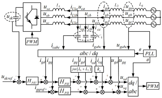
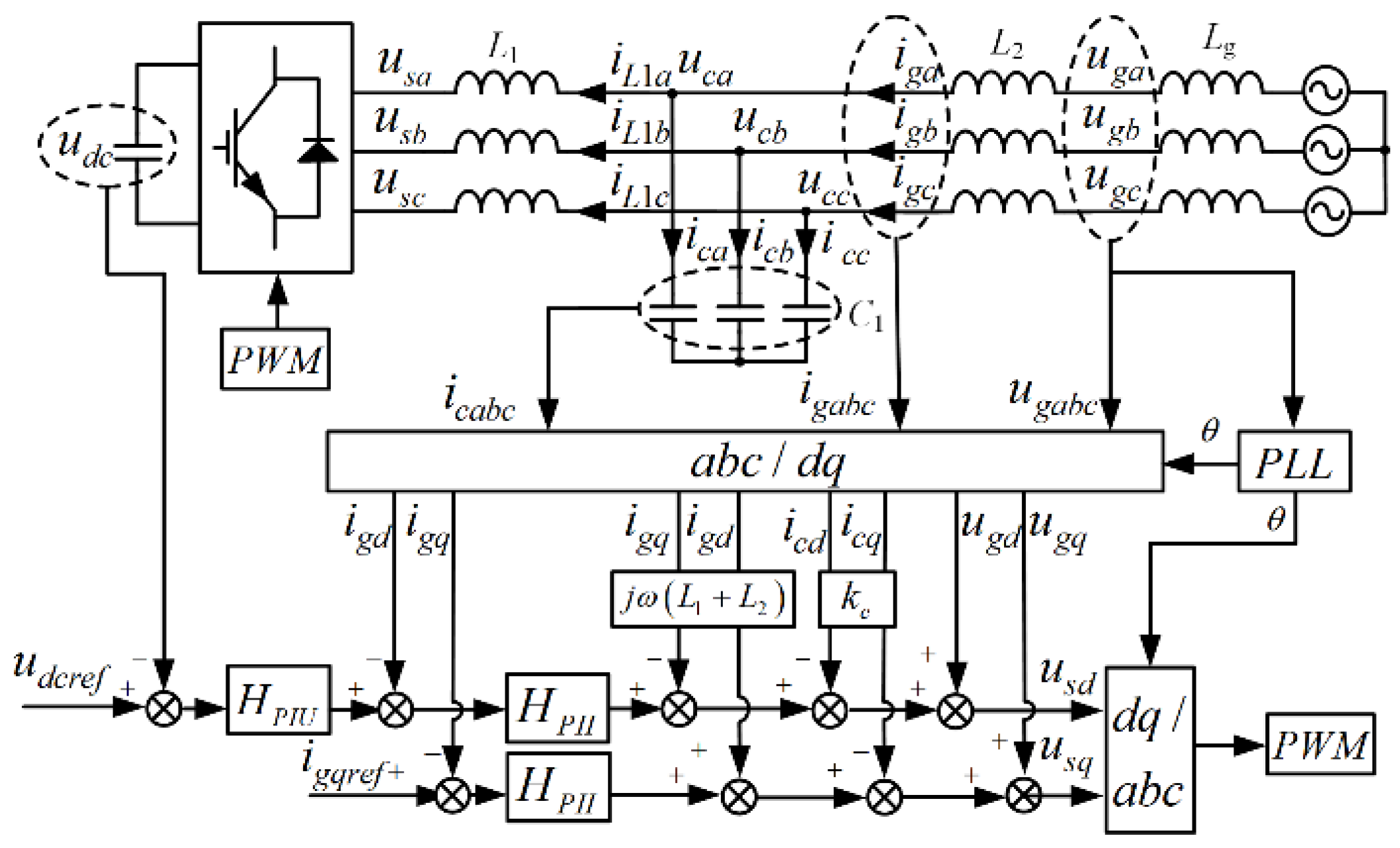
The topology and control structure of the LCL-type grid-connected converter studied in this paper are shown in Figure 1. In the figure, ugabc and usabc denote the point-of-common-coupling (PCC) voltage and the converter AC-side output voltage, respectively; igabc and icabc denote the three-phase grid current and the filter-capacitor current, respectively. igdq, icdq, and ugdq denote the d-axis and q-axis components of igabc, icabc, and ugabc after Park transformation. udc is the DC-side voltage of the converter. L1, L2 and C1 are the converter-side filter inductance, grid-side filter inductance, and filter capacitance of the LCL filter, respectively; Lg is the equivalent impedance of the AC grid. udcref and igdqref denote the references of the DC-side voltage and the grid current, respectively. HPIU and HPII are the PI controllers of the voltage loop and current loop, kc is the capacitor-current feedforward coefficient, and θ is the output phase angle of the PLL.
Figure 1.
Topology of the three-phase LCL-type grid-connected converter.
In the following modeling process, s denotes the Laplace operator, the prefix Δ denotes a small-signal perturbation, and the subscript 0 denotes a steady-state value.
2.2. Output-Admittance Modeling of the Grid-Connected Converter
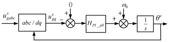
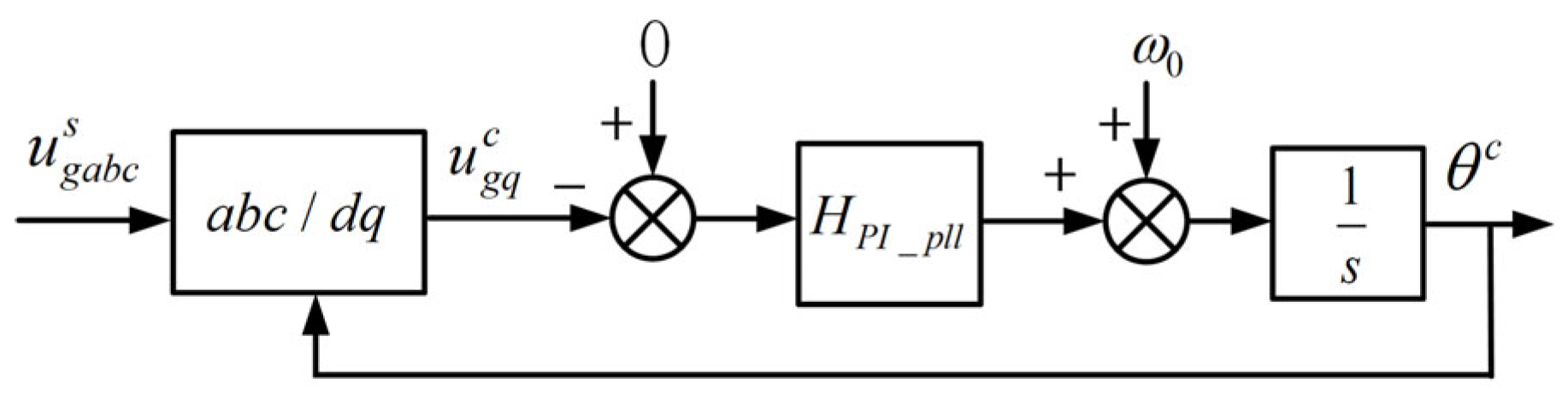
The PLL structure adopted in this paper is shown in Figure 2, where HPI_pll is the PI regulator of the PLL and ω0 is the grid fundamental angular frequency. According to the structure in Figure 2, the PLL output angle θ can be derived as the following expression.
Figure 2.
Block diagram of the PLL.
After small-signal linearization of (1), (2) is obtained.
where .
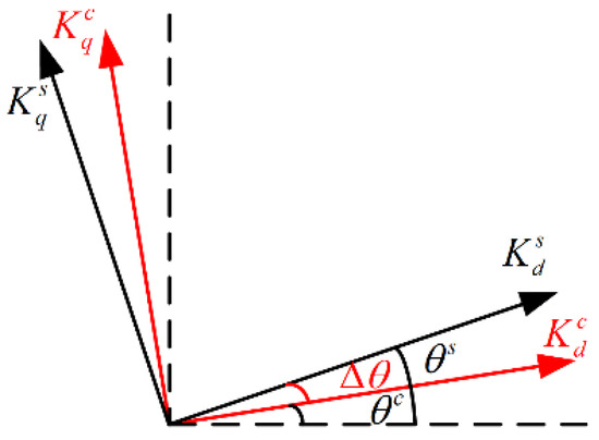
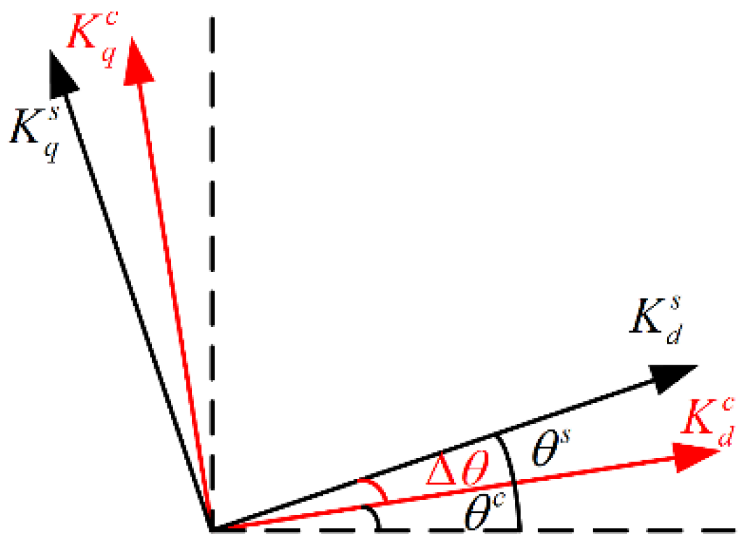
The presence of the PLL introduces two coordinate frames in small-signal modeling: the grid dq coordinate frame, whose variables are denoted by the superscript s, and the dq coordinate frame defined by the PLL output, whose variables are denoted by the superscript c. The relationship between the two coordinate frames is illustrated in Figure 3. Under steady-state conditions the two frames coincide, whereas when the system is subject to a small disturbance, the PLL tracking error is Δθ.
Figure 3.
The structure diagram of dq frames.
The state variables in the two coordinate frames can be transformed by (3).
where K denotes the state variables of the system. Combining Equations (2) and (3), the relational expression of small-signal state variables in the c-frame and s-frame is derived and presented in Equation (4). The detailed derivation is given in Equations (A1)–(A3) of Appendix A.
Combining the main circuit topology shown in Figure 1 and the small-signal linearization method, the relationships among small-signal state variables on the AC side of the converter system are derived and expressed in Equation (5). The detailed derivation is provided in Equations (A4)–(A9) of Appendix A.
Rearranging and simplifying Equation (5) yields Equation (6). The rearrangement process is presented in Equation (A10) of Appendix A.
where .
Assuming the input power Pin at the DC side of the converter is constant, the active power balance between the AC and DC sides is expressed as Equation (7). The detailed derivation is given in Equations (A11) and (A12) of Appendix A.
where .
The grid-connected converter adopts double closed-loop vector control consisting of a DC voltage outer loop and a current inner loop. The relationships between small-signal state variables are given in Equation (8), kc denotes the proportional feedback gain of the LCL filter capacitor current, which serves as the active damping coefficient for suppressing resonant peaks. The detailed derivation is shown in Equations (A13)–(A15) of Appendix A.
where , , .
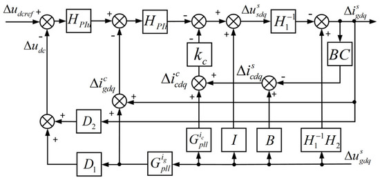
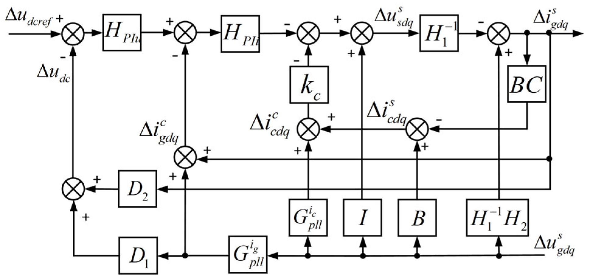
Combining (4)–(8), the small-signal block diagram of the LCL grid-connected converter shown in Figure 4 can be obtained.
Figure 4.
Small-signal block diagram of the three-phase LCL-type grid-connected converter.
Where and are the transformation matrices between the c-frame and s-frame. They are derived by substituting the variables K in Equation (5) with igdq and icdq, and their specific expressions are given as follows:
Taking Δigdq as the output and Δugdq as the input, the output-admittance model of the grid-connected converter can be obtained from Figure 4 as (11).
3. Admittance-Reshaping Method for the Grid-Connected Converter
3.1. Decoupling Compensation of the PLL and Voltage Outer Loop
In the control system, the asymmetric structures of the constant-DC-voltage outer-loop control and the PLL make the output-admittance model of the grid-connected converter asymmetric [26]. When ydd = yqq and ydq = −yqd, the system is called symmetric. In the asymmetric case, nonzero off-diagonal elements of the sequence-admittance model give rise to frequency coupling: a positive-sequence voltage disturbance at frequency fp not only produces a positive-sequence current response at fp, but also excites a negative-sequence current response at fp − 2fs, where fs is the grid frequency [27]. When background harmonics exist in the grid, the presence of frequency coupling increases the harmonic content of the grid current and deteriorates its quality. Therefore, to reduce the effect of background harmonics, a decoupling factor is introduced to decouple the frequency coupling in the converter admittance model.
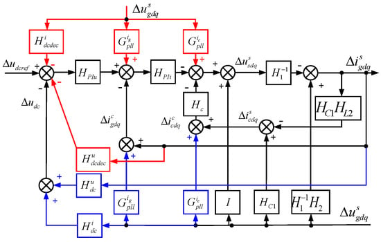
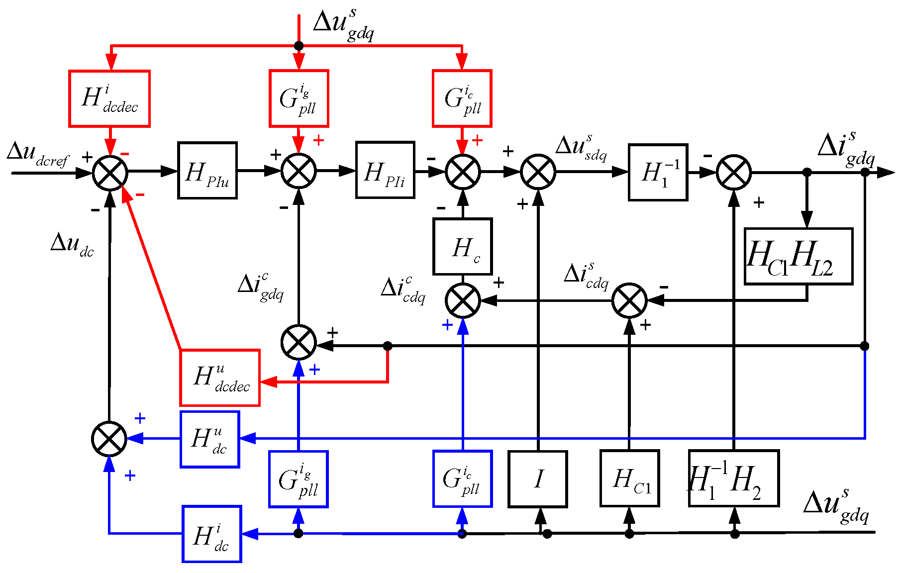
It can be observed from the admittance model of the grid-connected converter that all matrices in Y(s) are symmetric matrices with equal main diagonal elements and mutually opposite off-diagonal elements, except for the PLL-related matrices Gig pll, Gic pll and the voltage outer-loop matrices D1, D2. Accordingly, frequency coupling can be eliminated by introducing decoupling factors to convert asymmetric matrices into symmetric ones. As shown in Equation (12), D1dec and D2dec are introduced to make D1 + D1dec and D2 + D2dec symmetric matrices. Meanwhile, a compensation term opposite to the branch affected by the PLL is added to the current loop to counteract the PLL’s influence. The detailed compensation scheme is illustrated by the red branches in Figure 5.
Figure 5.
Structure of the decoupling compensation scheme.
The specific compensation structure is illustrated by the red branches in Figure 5. The red part represents the added compensation factor, and the blue part denotes the components to be modified in the original model.
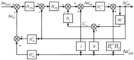
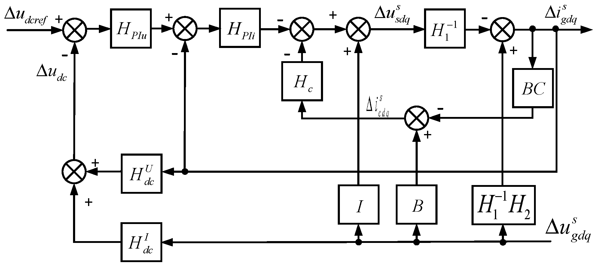
The converter small-signal block diagram can be simplified to that shown in Figure 6.
Figure 6.
Simplified small-signal block diagram after decoupling compensation.
Based on Figure 6, the output-admittance model of the grid-connected converter after decoupling compensation is derived as Equation (13). The elements of the corresponding matrix are provided in Equation (A20) of Appendix A.
where .
Since all matrices in (13) are symmetric, the converter admittance model also becomes symmetric, the off-diagonal elements become zero, and the frequency coupling is eliminated.
3.2. Grid-Voltage Feedforward Compensation
Under weak-grid conditions, the grid equivalent impedance is large and the short-circuit ratio is low. Such conditions amplify background harmonics and also readily interact with the control structure of the grid-connected converter, thereby triggering broadband oscillations. Therefore, on the basis of the frequency-coupling decoupling compensation proposed in the previous subsection, the converter output admittance is further reshaped to optimize the admittance characteristics and enhance the stability of the grid-connected system under weak-grid conditions. In a weak grid, the grid-voltage feedforward signal contains the voltage drop across the grid impedance, which introduces an additional positive-feedback path for the grid current in the control structure, reduces the system phase margin, and causes the output admittance to exhibit negative-admittance characteristics [28].
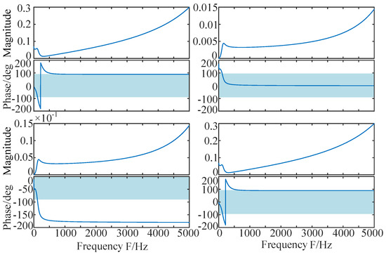
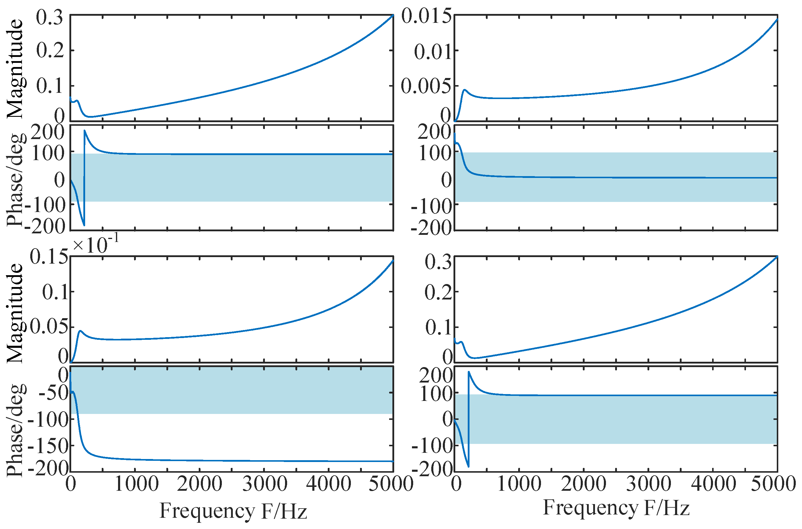
Figure 7 plots the Bode diagrams of the four elements of the output-admittance matrix after decoupling compensation. It can be seen that the converter admittance matrix is symmetric, with identical diagonal elements and opposite off-diagonal elements; however, a non-passive region with a negative real part still exists, so the system cannot operate stably under weak-grid conditions.
Figure 7.
Bode plots of the output-admittance elements after decoupling compensation.
Rewriting Y1(s) yields Equation (14).
where ,
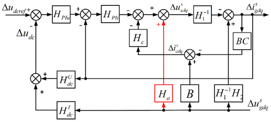
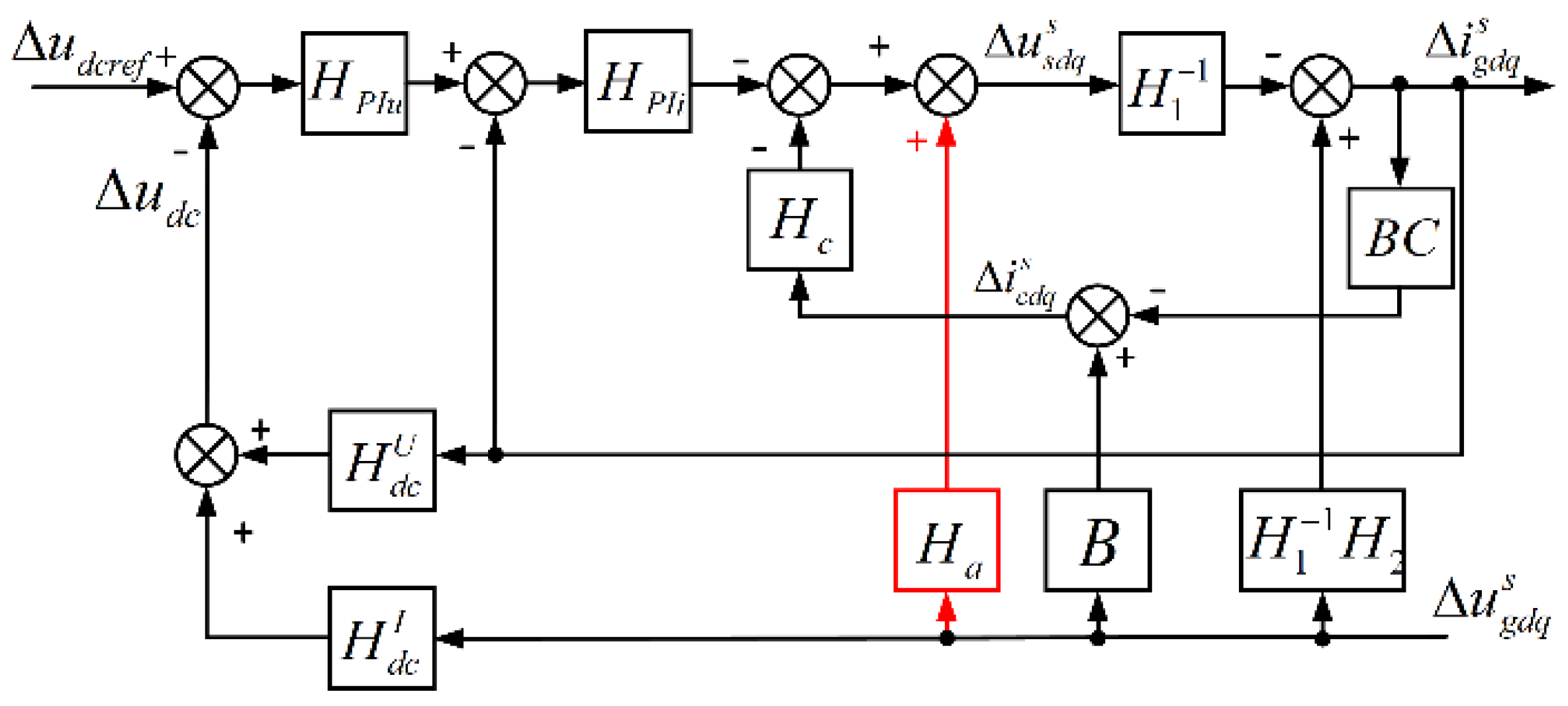
Because H1(s) in the expression of Y1(s) is mainly affected by the grid-voltage feedforward in the medium- and low-frequency ranges [29], the phase margin of Y1(s) can be improved by correcting H1(s). Therefore, a first-order inertial link Ga(s) is introduced into the d-axis and q-axis grid-voltage feedforward channels as a phase-correction function to eliminate the negative damping introduced by grid-voltage feedforward. The compensation scheme is shown in Figure 8. The red part indicates the added compensation factor.
Figure 8.
Structure of the grid-voltage feedforward compensation scheme.
Ga(s) is given by (15), where ka is the proportional gain coefficient and ωα is the corner frequency. The compensation matrix Ha is then defined by (16).
After feedforward compensation is introduced, the output admittance Y2(s) is given by (17), and its detailed expression is listed in (A21) of Appendix A.
The compensated Y2(s) is a symmetric matrix, and the magnitude of its diagonal elements is much larger than that of the off-diagonal elements. Therefore, the diagonal element Y2dd dominates system stability. Decomposing Y2dd yields two sub-admittances, Yi and Yua, which are related to the current loop and the voltage feedforward, respectively, as shown in (18).
Since the non-passive frequency band that needs correction for the output admittance Y1(s) is below 2000 Hz, and the voltage harmonics in public power grids are mainly distributed below the 40th order of fundamental frequency harmonics [30], the magnitude of the output admittance is minimized within the designed frequency range to guarantee the background harmonic suppression capability of the grid-voltage feedforward link. Accordingly, the corner frequency is set as ωa = 2π × 2000 rad/s [31].
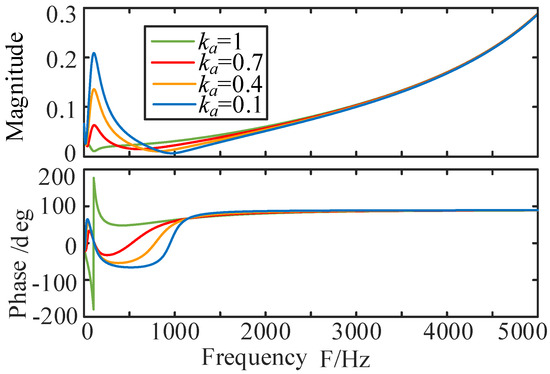
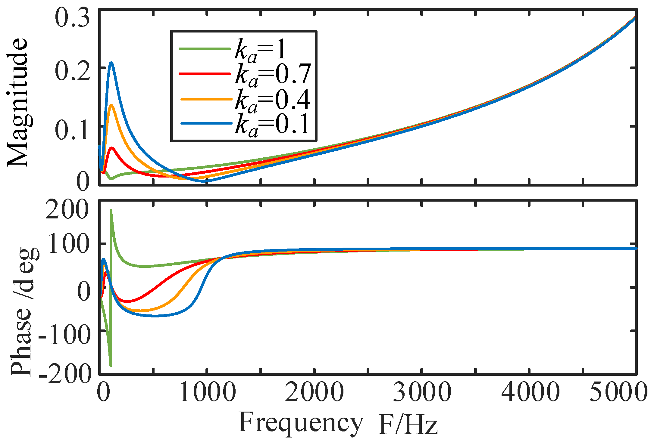
The output admittance Y2dd consists of two sub-admittances associated with the current loop and grid-voltage feedforward, which are denoted as Yi and Yua respectively. Figure 9 shows the Bode plot of Y2dd for different values of ka. As ka decreases, the negative-damping region of Y2dd disappears and Y2dd moves into the passive region; however, the magnitude of Y2dd increases as ka decreases. This increase may amplify background harmonics and thus degrade power quality. Therefore, the proportional gain coefficient ka must be properly designed.
Figure 9.
Bode plot of Y2dd for different values of ka.
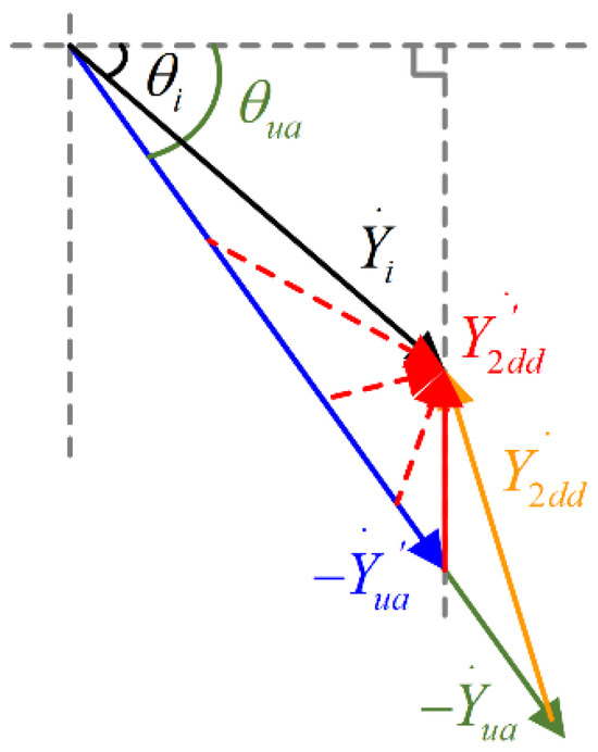
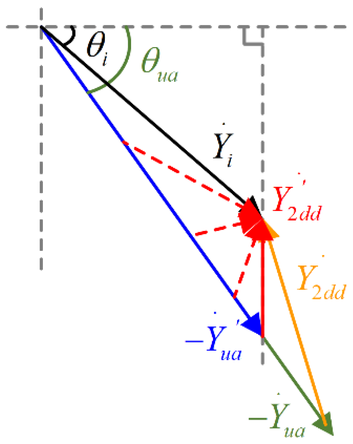
The combined phasor diagram of Yi, Yua and the output admittance Y2dd is shown in Figure 10. As indicated by the mathematical expression, the magnitude of Yua is directly proportional to ka. When the proportional gain ka is adjusted, both the voltage feedforward admittance Yua and the output admittance Y2dd will vary, which are denoted as Yua’ and Y2dd’.
Figure 10.
Synthesized phasor diagram of the sub-admittances Yi and Yua and the output admittance Y2dd.
We take the value of ka at the critical phase state of Y2dd as the upper limit. When ka is lower than this upper limit, the phase of the admittance always lies within the passive region of [−90°,90°]. Based on the trigonometric relationship under the critical condition, the constraint for ka is derived as follows:
where .
Combining Equation (19) and the foregoing conclusion that the magnitude of Y2dd increases as ka decreases, we select the maximum value of ka that satisfies Equation (19) to prevent excessive Y2dd magnitude from deteriorating power quality. In this work, ka is set to 0.7.
3.3. Analysis of the Compensated Admittance Model
To facilitate analysis, the transformation matrix F is adopted to convert the compensated output-admittance model Y2(s) of the converter in the dq frame into the sequence-admittance model Y2pn(s) [32].
where .
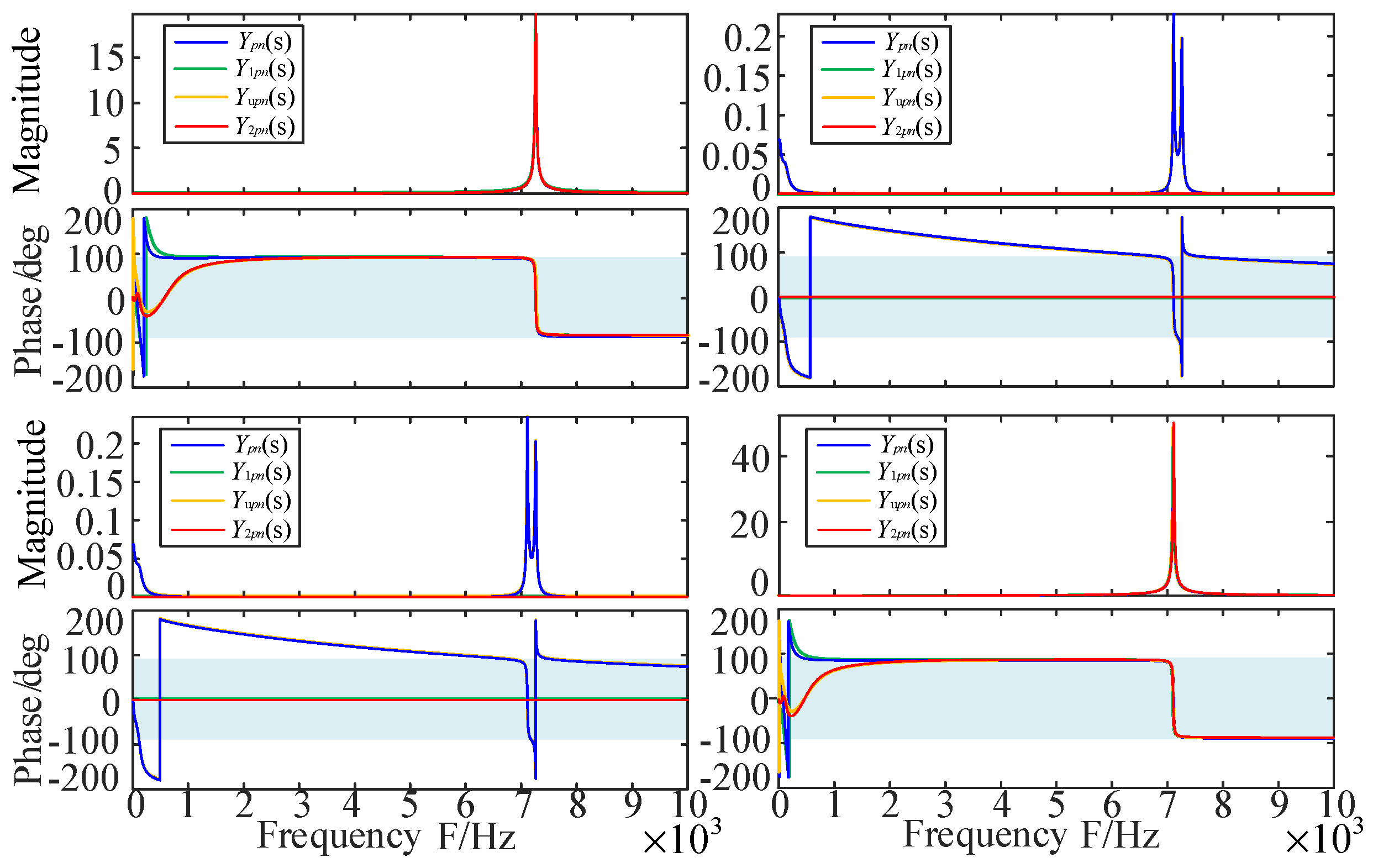
Figure 11 compares the Bode plots of the sequence-admittance elements before and after compensation, where Ypn(s), Y1pn(s), Yupn(s), and Y2pn(s) denote the output sequence admittance before compensation, with only the decoupling factor added, with only the feedforward compensation link added, and with the compensation proposed in this paper added, respectively.
Figure 11.
Comparison of the Bode plots of the sequence-admittance elements before and after compensation.
It can be seen from Figure 11 that when only the decoupling factor or only the voltage-feedforward compensation link is introduced, the output sequence admittance still contains regions with negative real parts and therefore still affects system stability. When the two compensation strategies are applied in a coordinated manner, the off-diagonal elements of the sequence-admittance matrix become zero, which verifies the effectiveness of the proposed decoupling method. In addition, the phases of the sequence-admittance elements remain within [−90°,90°] over the entire frequency range, meaning that the real part of the output sequence admittance is positive over the full band and the stability of the system under weak-grid conditions is improved.
4. Simulation and Experimental Verification
4.1. Simulation Verification
To verify the effectiveness of the proposed compensation scheme, a three-phase LCL-type grid-connected converter model as shown in Figure 1 is built in MATLAB/Simulink (2023a). The simulation parameters are listed in Table A1 of Appendix B.
4.1.1. Verification of the Theoretical Admittance Model
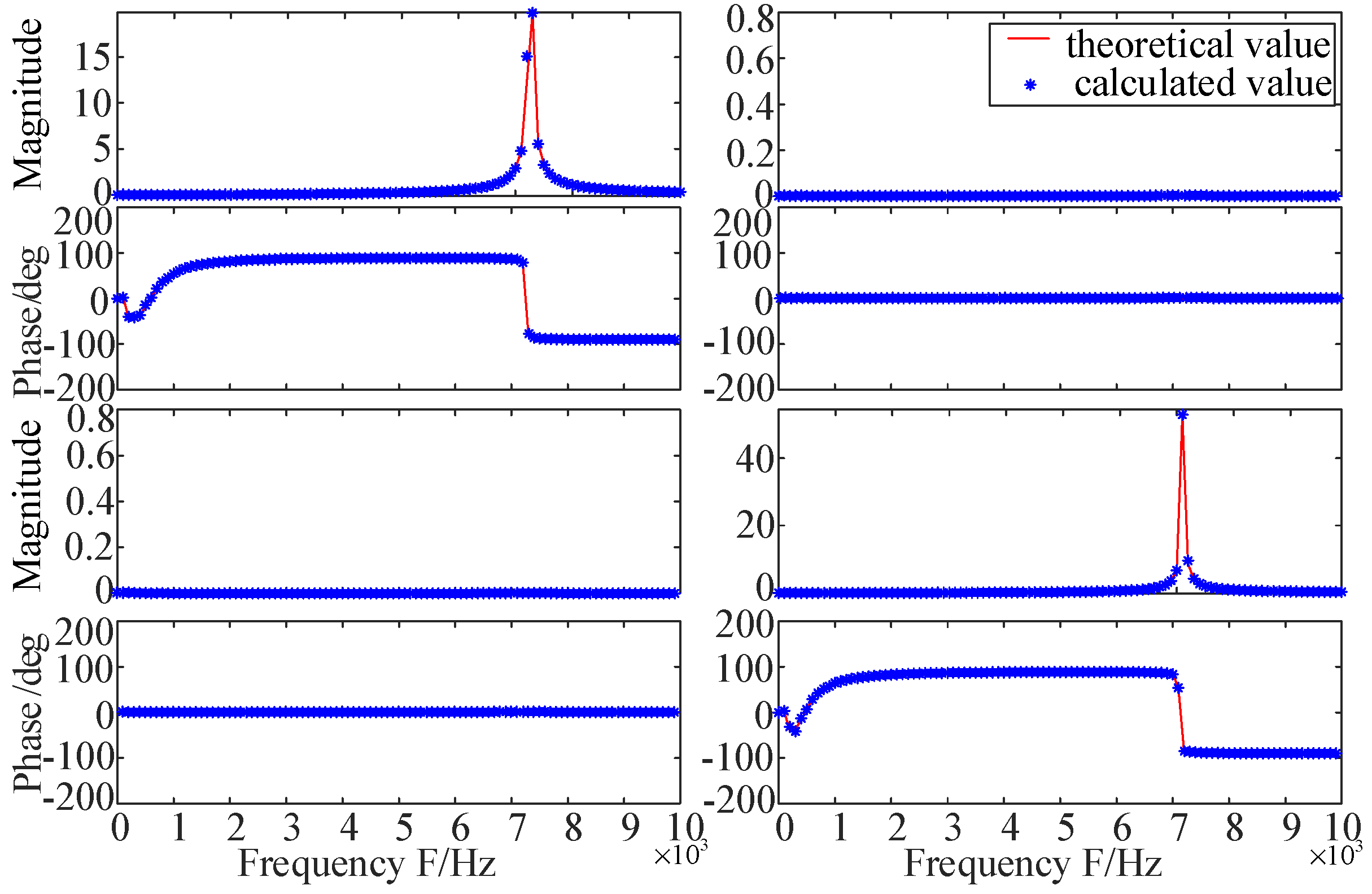
Frequency sweep analysis is performed on the simulation model. Figure 12 compares the measured and theoretically calculated results of the sequence-admittance model for the compensated grid-connected converter. It can be observed that the two curves are basically coincident, which verifies the accuracy of the theoretical model.
Figure 12.
Comparison of magnitude-frequency and phase-frequency curves of the compensated converter sequence admittance.
4.1.2. Verification of Background Harmonic Suppression and Stability Improvement Performance
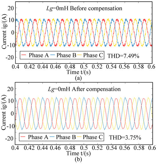
To verify the capability of the designed compensation method to mitigate the impact of grid background harmonics, the 5th, 7th, 13th, 17th and 19th harmonics with harmonic contents of 4.5%, 3.5%, 2.5%, 1.5% and 1% are injected into the grid voltage. The output current waveforms of the converter before and after applying the proposed compensation are presented in Figure 13 under harmonic voltage disturbances.
Figure 13.
Grid-connected current waveforms before and after applying compensation under harmonic voltage injection: (a) After compensation; (b) Before compensation.
It can be seen that the grid-connected current suffers from severe distortion with a THD of 7.49% before compensation. After adopting the proposed method, the current quality is improved, and the THD drops to 3.75%.
The output-admittance model indicates that the system is a two-input two-output system, so the generalized Nyquist criterion is adopted for stability analysis. The return ratio matrix is defined as the product of the converter output-admittance matrix Y and the grid impedance matrix Zg. The stability of the grid-connected system is judged according to the eigenvalue loci of the return ratio matrix.
The grid impedance matrix is expressed as:
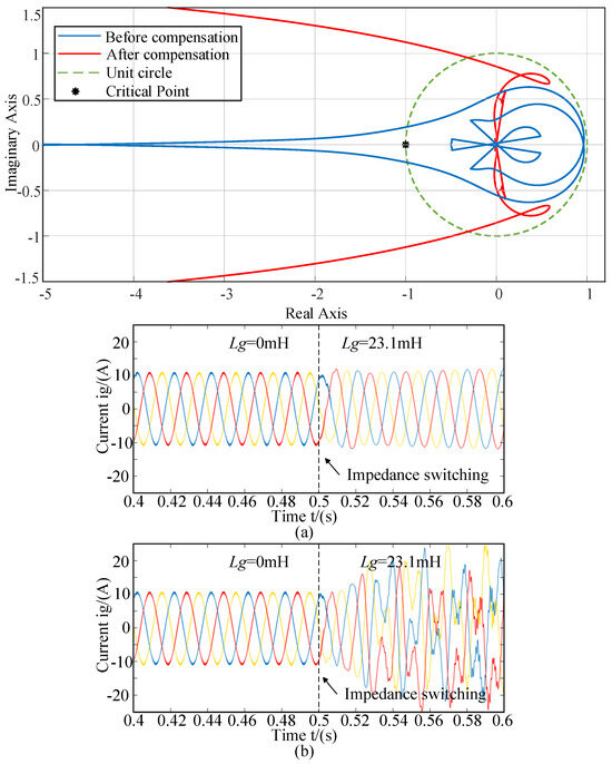
Figure 14 presents the Nyquist curves and simulated grid-connected current waveforms when the grid inductance increases from 0 mH to Lg = 23.1 mH (SCR = 2).
Figure 14.
Grid-connected current waveforms and eigenvalue loci of the return ratio matrix before and after compensation under SCR = 2 (The yellow, blue and red waveforms represent the currents of phases A, B and C, respectively): (a) After compensation; (b) Before compensation.
It can be seen that when the grid inductance Lg = 23.1 mH, the Nyquist curve encloses the point (−1,0) before compensation, indicating system instability. After compensation, the Nyquist curve no longer surrounds (−1,0), and the system becomes stable. The grid-connected current waveforms are consistent with the results of the generalized Nyquist criterion, which verifies that the proposed compensation method effectively improves the stability of grid-connected converters under weak grid conditions.
4.1.3. Sensitivity and Robustness Analysis Under Different Operating Conditions
Sensitivity Analysis of PLL Bandwidth
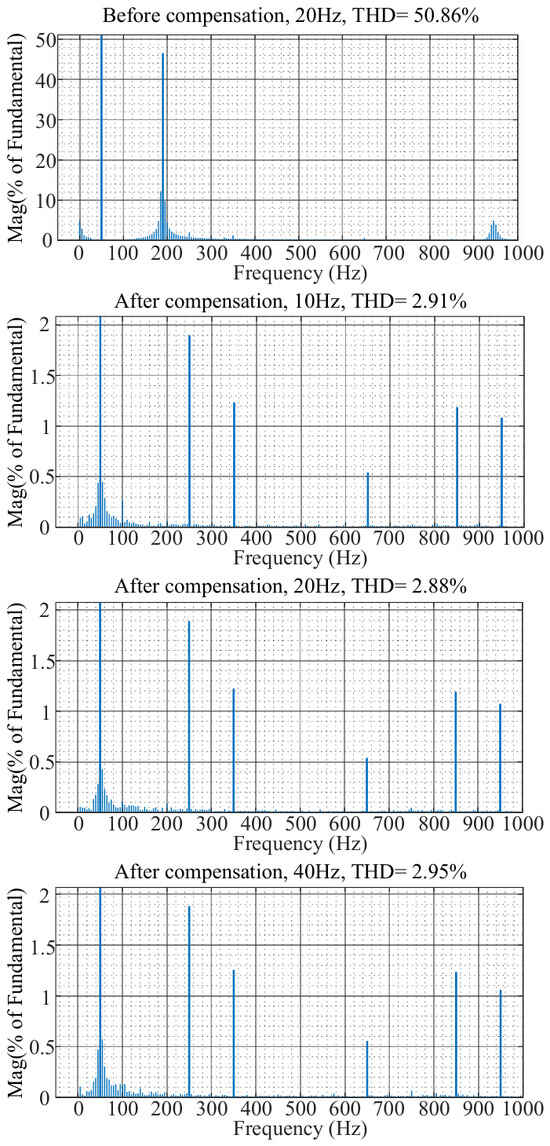
Under the weak grid condition with Lg = 23.1 mH (SCR = 2), four groups of simulations are carried out. For the system with the proposed compensation, the PLL bandwidth is set to 10 Hz, 20 Hz and 40 Hz respectively; for the uncompensated system, the PLL bandwidth is set to 20 Hz. The 5th, 7th, 13th, 17th and 19th harmonics with harmonic contents of 4.5%, 3.5%, 2.5%, 1.5% and 1% are injected into the grid voltage. The FFT diagrams of grid-connected current for the four simulation groups are shown in Figure 15.
Figure 15.
FFT diagrams of grid-connected current under different PLL bandwidths.
As illustrated in the figure, the THD values of grid-connected current for the three compensated cases are 2.91%, 2.88% and 2.95% respectively. The system remains stable and the grid-connected current meets power quality requirements. By contrast, the uncompensated system suffers from severe current distortion and becomes unstable. This demonstrates that the harmonic suppression performance of the proposed method has low sensitivity to PLL bandwidth.
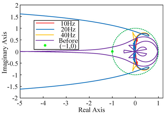
Figure 16 shows the eigenvalue loci of the return ratio matrix for the grid-connected system in the four simulation cases.
Figure 16.
Eigenvalue loci of the return ratio matrix for the grid-connected system under different PLL bandwidths.
It can be observed that the eigenvalue loci of the three compensated cases do not enclose the point (−1,0), and only present slight differences inside the unit circle with varying bandwidths. According to the generalized Nyquist criterion, the system maintains stable operation under weak grid conditions. In comparison, the eigenvalue locus of the uncompensated system encircles (−1,0), leading to system instability. The results prove that the stability improvement achieved by the proposed method is insensitive to PLL bandwidth variations.
The simulation results indicate that the proposed method can effectively suppress background harmonics and enhance system stability with no obvious current distortion when the PLL bandwidth fluctuates within a reasonable range. This verifies the excellent robustness of the method against PLL parameter variations, and further improves its theoretical rigor and engineering applicability.
Analysis on Control Parameter Disturbance
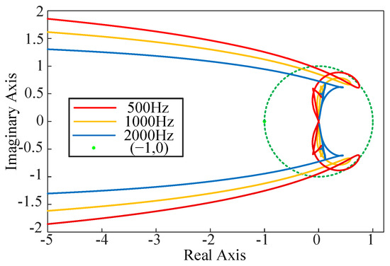
Under the weak grid condition of Lg = 23.1 mH (SCR = 2), three groups of simulations are conducted with the current loop bandwidth set to 500 Hz, 1000 Hz and 2000 Hz after applying the proposed compensation. The same harmonics as above are injected into the grid voltage. The FFT diagrams of grid-connected current are presented in Figure A1 of Appendix A.
The results show that the THD of grid-connected current remains below 5% when the current loop bandwidth varies from 500 Hz to 2000 Hz, and gradually decreases with the increase in bandwidth. It is verified that the proposed method possesses strong robustness against variations in current loop parameters and can well adapt to control parameter disturbances. Figure 17 depicts the eigenvalue loci of the return ratio matrix under the three different current loop bandwidths.
Figure 17.
Eigenvalue loci of the return ratio matrix for the grid-connected system under different current loop bandwidths.
It can be seen that the eigenvalue loci gradually converge inward as the current loop bandwidth increases, yet none of them enclose the point (−1,0). In accordance with the generalized Nyquist criterion, the system stays stable throughout the tests. This verifies that the proposed method maintains favorable robustness against disturbances of current loop control parameters in weak grid scenarios.
Analysis on Uncertain Grid Conditions
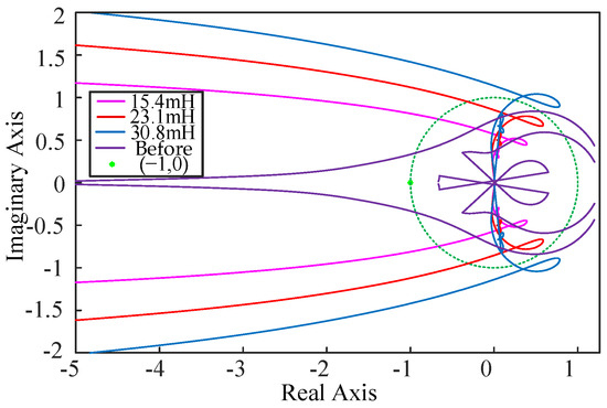
To verify the robustness of the designed admittance-reshaping method in terms of background harmonic suppression and stability improvement under uncertain grid impedance, three operating conditions are established to simulate wide variations of grid impedance: ideal grid (Lg = 0 mH), weak grid (Lg = 23.1 mH, SCR = 2) and extremely weak grid (Lg = 30.8 mH, SCR = 1.5). The same harmonics as aforementioned are injected into the grid voltage under the three conditions, and the corresponding FFT diagrams of grid-connected current are shown in Figure A2 of Appendix A.
As observed from the results, for the ideal grid without compensation, the THD of grid-connected current reaches 7.49% with severe distortion, which fails to meet power quality standards. After adopting the admittance-reshaping method, the THD drops to 3.75% with obviously reduced harmonics. Under weak grid and extremely weak grid conditions, the THD values after compensation are 2.88% and 2.17% respectively. The above results demonstrate that the proposed method can effectively suppress background harmonics against wide-range variations of grid impedance.
Figure 18 presents the eigenvalue loci of the return ratio matrix for the grid-connected system before and after admittance reshaping at SCR = 3, as well as those after reshaping at SCR = 2 and SCR = 1.5.
Figure 18.
Eigenvalue loci of the return ratio matrix under different grid impedances.
It can be seen that for the grid condition with SCR = 3, the eigenvalue locus encloses the point (−1,0) before compensation, which indicates system instability according to the generalized Nyquist criterion. After compensation, the locus no longer surrounds (−1,0) and the system operates stably. When the grid impedance further increases to 23.1 mH and 30.8 mH, the eigenvalue loci still avoid encircling (−1,0), and the system remains stable. The above analysis proves that the proposed compensation method can effectively guarantee system stability under wide-range grid impedance variations, ranging from ideal grid, weak grid to extremely weak grid.
Analysis of Control Delay Influence
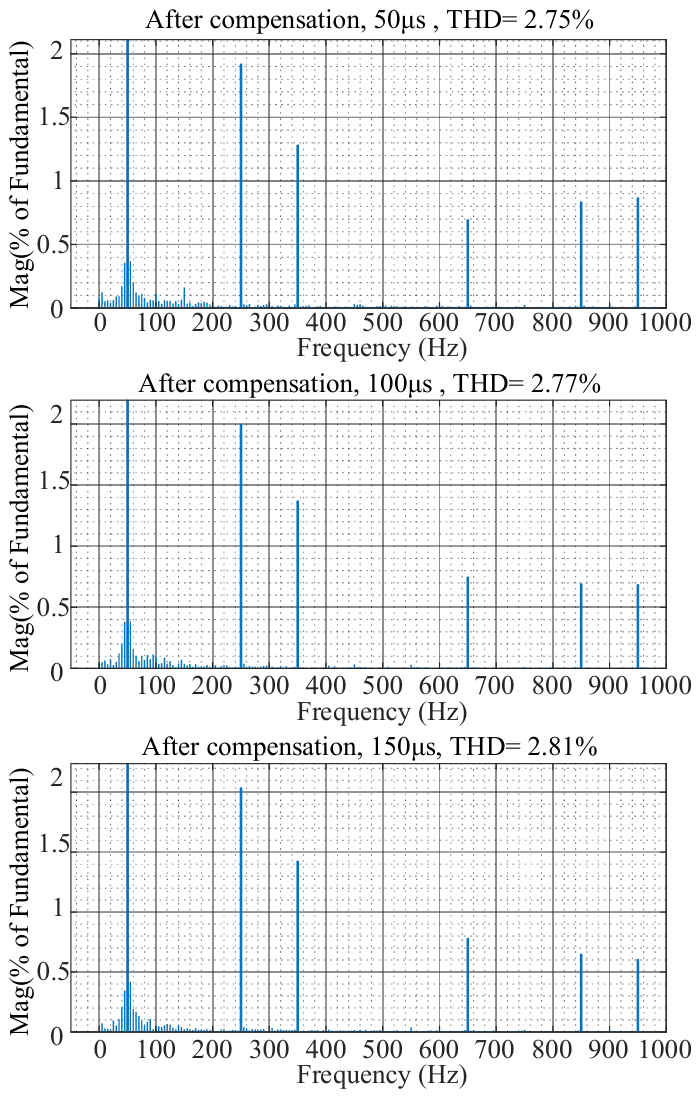
To verify the robustness of the designed admittance-reshaping method against inherent digital control delays, simulations are carried out under the weak grid condition of Lg = 23.1 mH (SCR = 2) with control delays set to 50 μs, 100 μs and 150 μs, covering typical and severe delay scenarios in practical engineering. The FFT diagrams of grid-connected current under the three conditions are shown in Figure A3 of Appendix A.
The results show that the grid-connected current maintains good sinusoidal quality within the set delay range, with THD values of 2.75%, 2.77% and 2.81% respectively. The THD rises slightly as the delay increases, and the system stays stable in all cases. It is demonstrated that the proposed compensation scheme has excellent robustness against inherent digital control delays in terms of harmonic suppression and stability enhancement.
Verification Under Unbalanced Grid Conditions
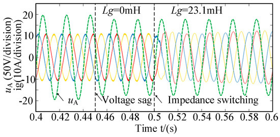
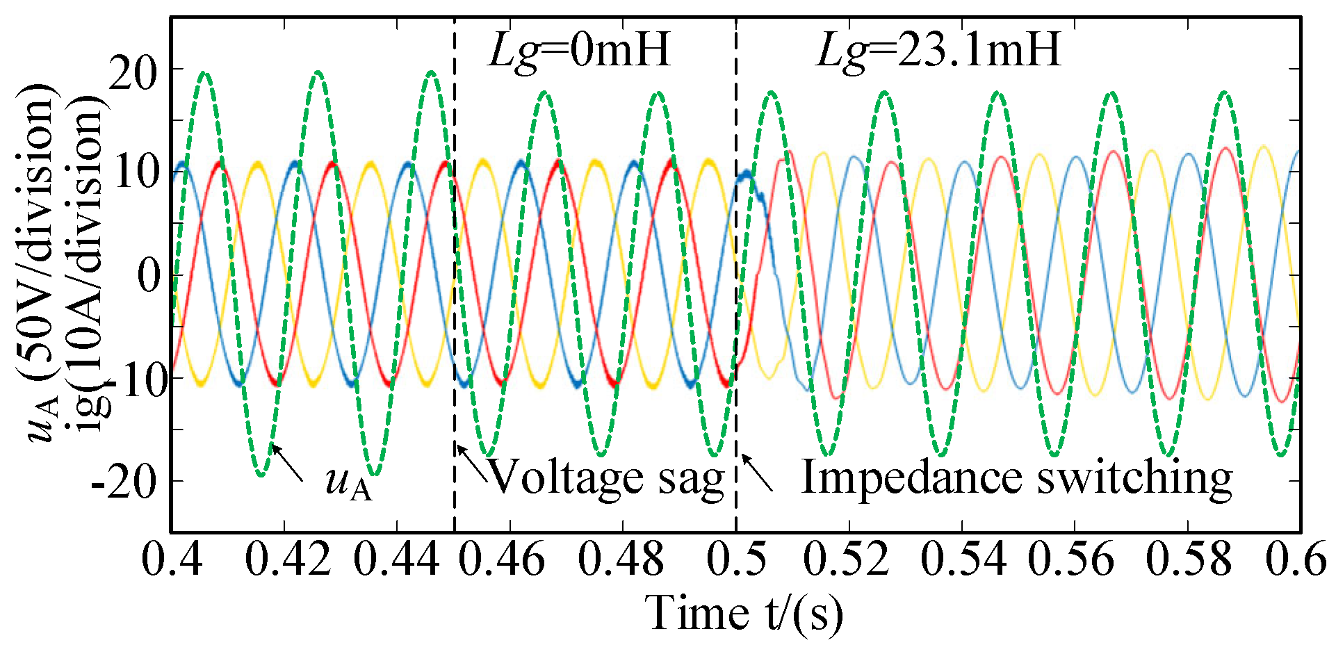
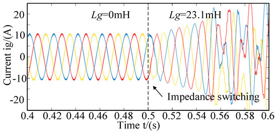
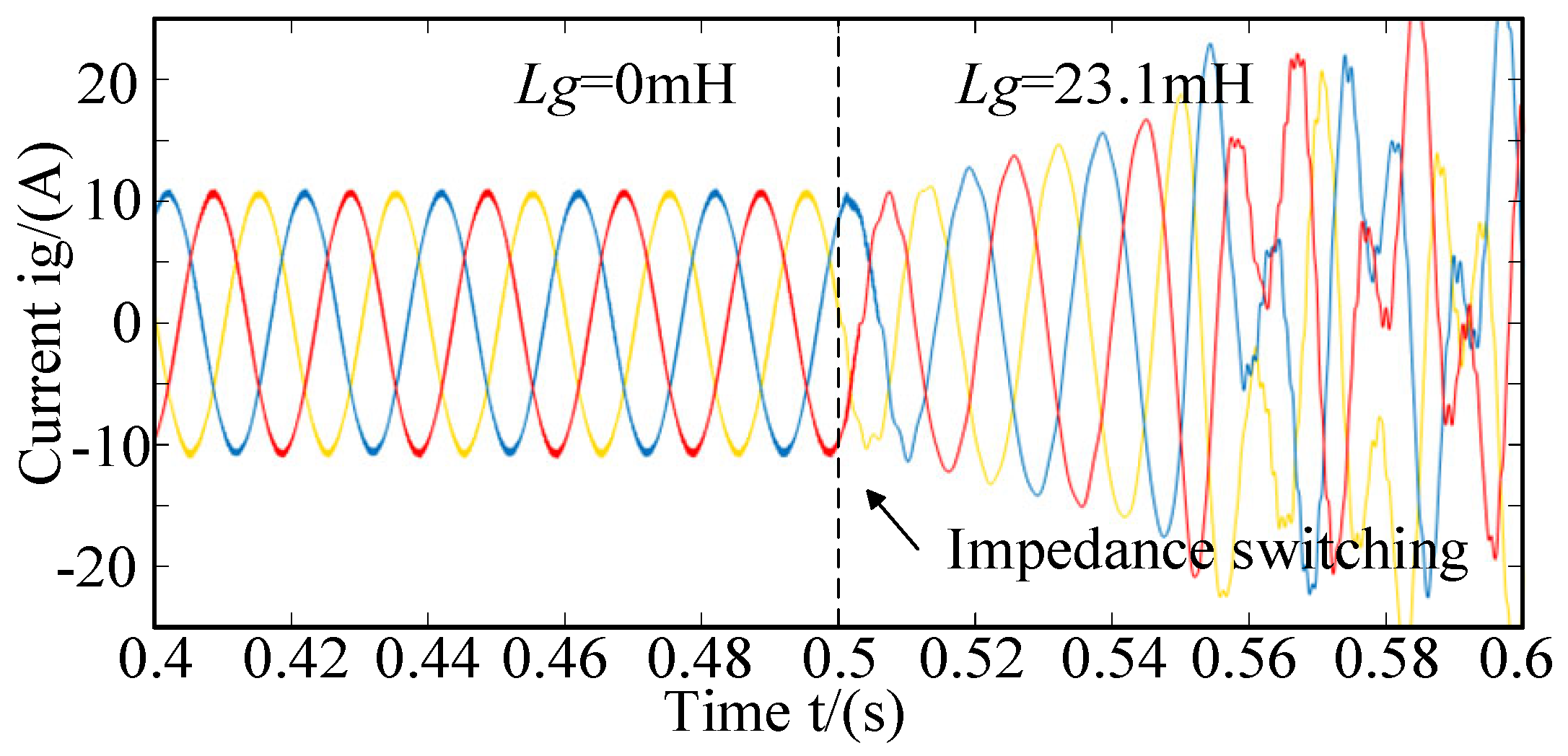
To validate the effectiveness of the proposed compensation method under unbalanced grid conditions, the voltage of Phase A is dropped by 10% at t = 0.45 s. Meanwhile, the grid impedance is switched from the ideal grid to the weak grid at t = 0.5 s. The waveforms of grid-connected current and Phase A voltage are illustrated in Figure 19.
Figure 19.
Waveforms of Phase A voltage and grid-connected current during impedance switching under unbalanced grid conditions (The yellow, blue and red waveforms represent phase-A, phase-B and phase-C currents, respectively).
It can be observed that the system remains stable after the voltage sag of Phase A and the subsequent switch to weak grid. This verifies the effectiveness of the proposed compensation method under unbalanced grid conditions.
4.1.4. Comparative Analysis with Existing Methods
Reference [28] proposes an admittance-reshaping strategy for grid-connected converters, which reduces the magnitude of sequence admittance to suppress grid background harmonics. To quantitatively evaluate the performance of the control strategy in this paper, a simulation model is established using the same system parameters as in the literature. Comparative simulations are conducted from two aspects including harmonic suppression and stability margin under weak grid conditions, so as to intuitively analyze the advantages and disadvantages of the two admittance optimization schemes.
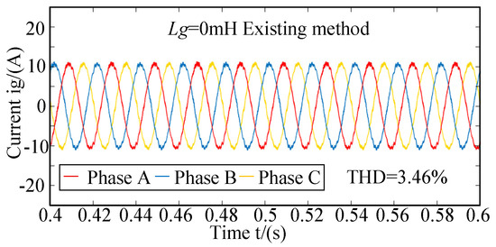
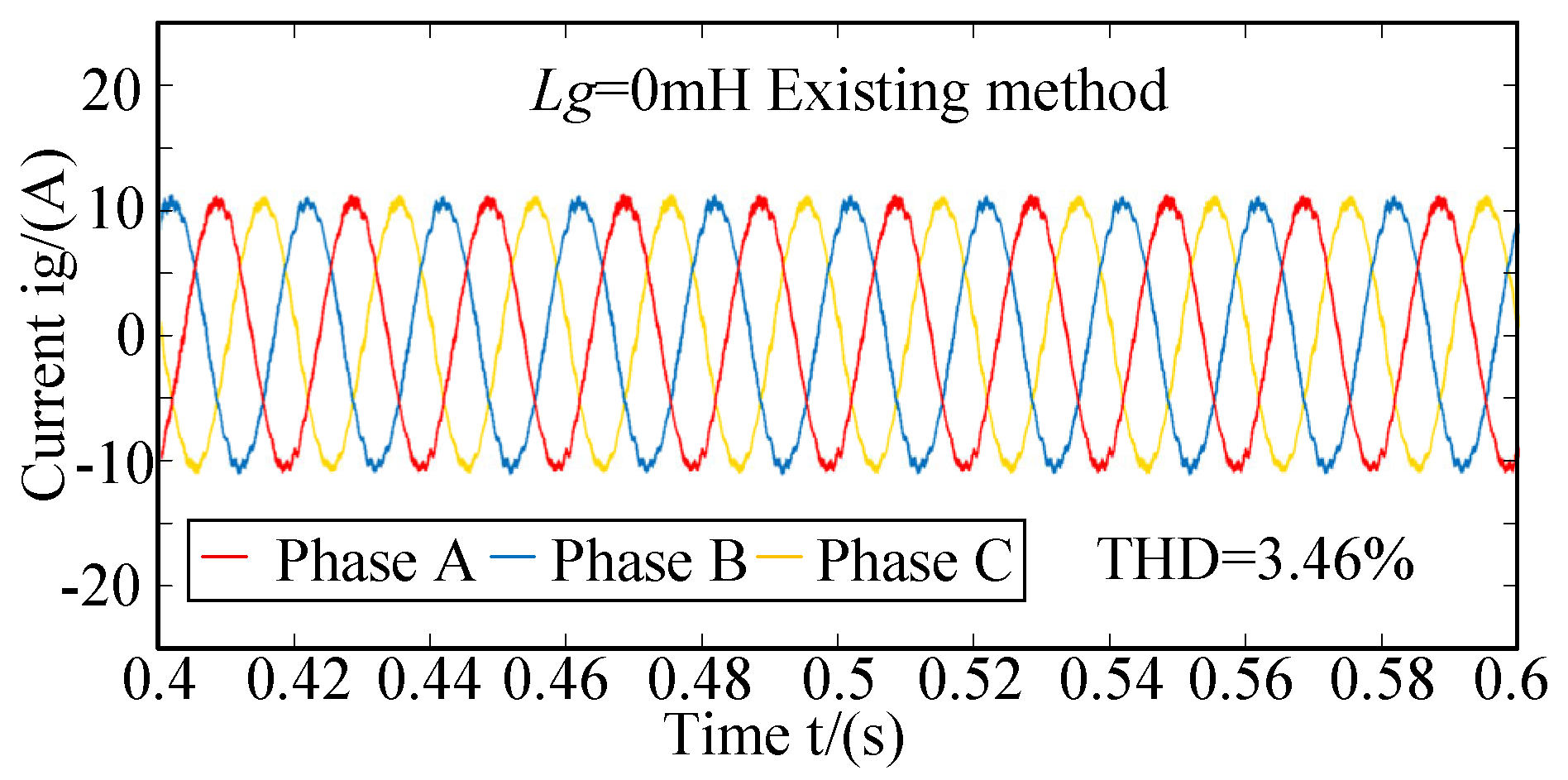
Under the ideal grid condition, the 5th, 7th, 13th, 17th and 19th harmonics with harmonic contents of 4.5%, 3.5%, 2.5%, 1.5% and 1% are injected into the grid voltage. The grid-connected current waveforms obtained by the method in reference [28] are shown in Figure 20.
Figure 20.
Grid-connected current waveform with harmonic injection using the compensation method in the reference.
Combined with the waveforms in Figure 13 for the uncompensated system and the proposed method in this paper, it can be found that the current waveform is severely distorted by background harmonics with a THD of 7.49% without admittance reshaping. The proposed method evidently reduces harmonic components and produces smooth current waveforms, with the THD decreasing to 3.75%. The method in reference suppresses background harmonics by reducing the admittance magnitude, achieving a THD of 3.46%. The comparison indicates that both methods can effectively mitigate grid background harmonics with comparable performance.
Figure 21 shows the grid-connected current waveforms of the reference method when the operating condition is switched from the ideal grid to the weak grid with Lg = 23.1 mH (SCR = 2).
Figure 21.
Grid-connected current waveform after grid impedance switching using the compensation method in the reference (The yellow, blue and red waveforms represent phase-A, phase-B and phase-C currents, respectively).
Combined with the results in Figure 14, the system becomes unstable and the current is severely distorted after grid impedance switching for both the uncompensated scheme and the method in the reference. In contrast, the system maintains stable operation with the proposed compensation method. The simulation results verify that the proposed method has better adaptability to wide-range variations of grid impedance.
4.2. Experimental Verification
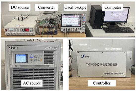
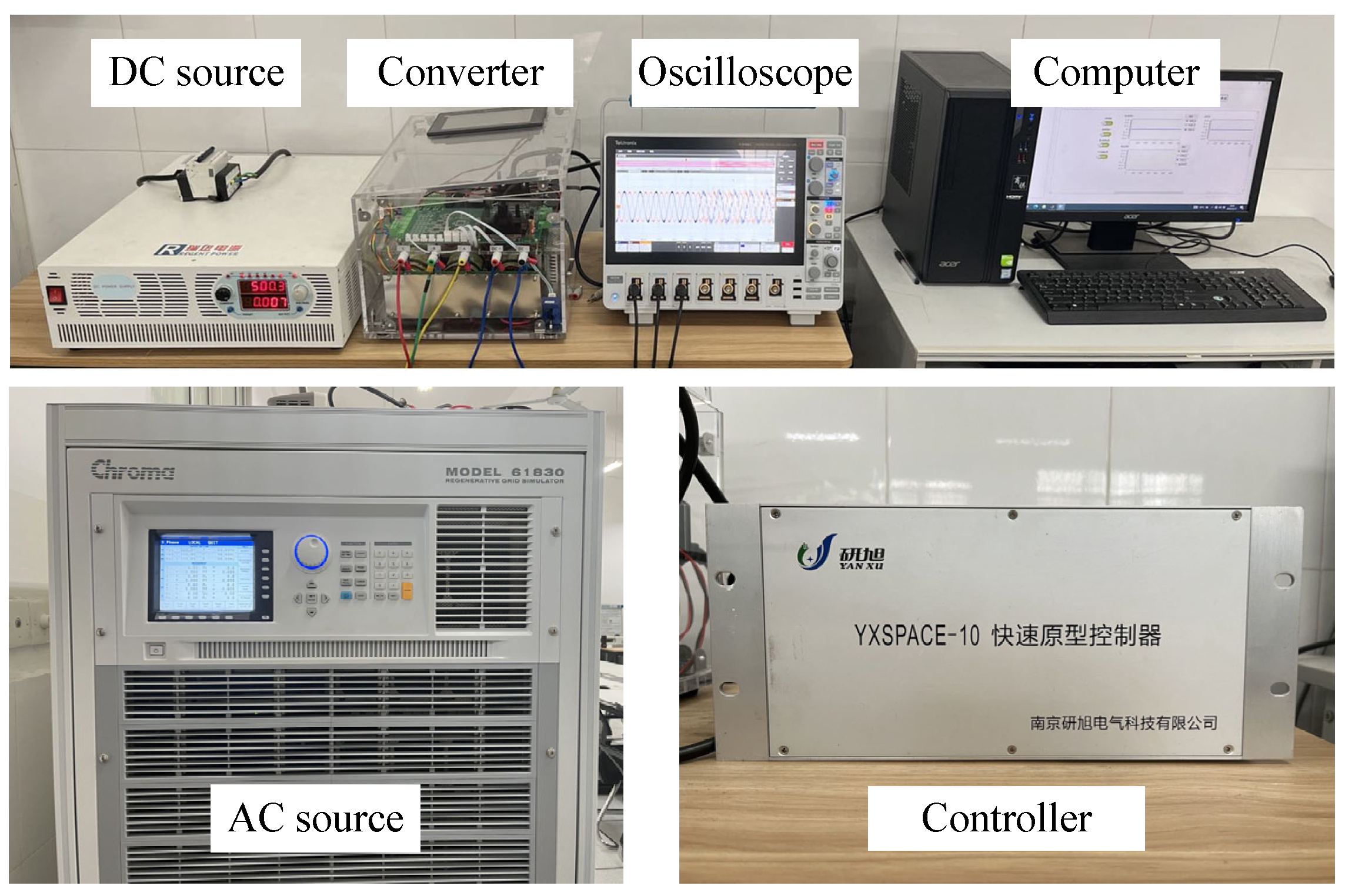
To verify the effectiveness of the proposed method, a 2.5 kW three-phase LCL-type grid-connected converter experimental prototype was constructed. The experimental setup is shown in Figure 22, and the experimental parameters are consistent with those listed in Appendix B, Table A1. The experimental equipment information is as follows: DC source and converter (ITECH Electronics, Nanjing, China), oscilloscope (Tektronix, Inc., Beaverton, OR, USA), AC source (Chroma ATE Inc., Taoyuan, Taiwan, China), controller (Yanxu Electric Technology Co., Ltd., Nanjing, China).
Figure 22.
Experimental platform.
4.2.1. Verification of Background Harmonic Suppression Effect
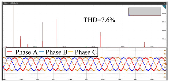
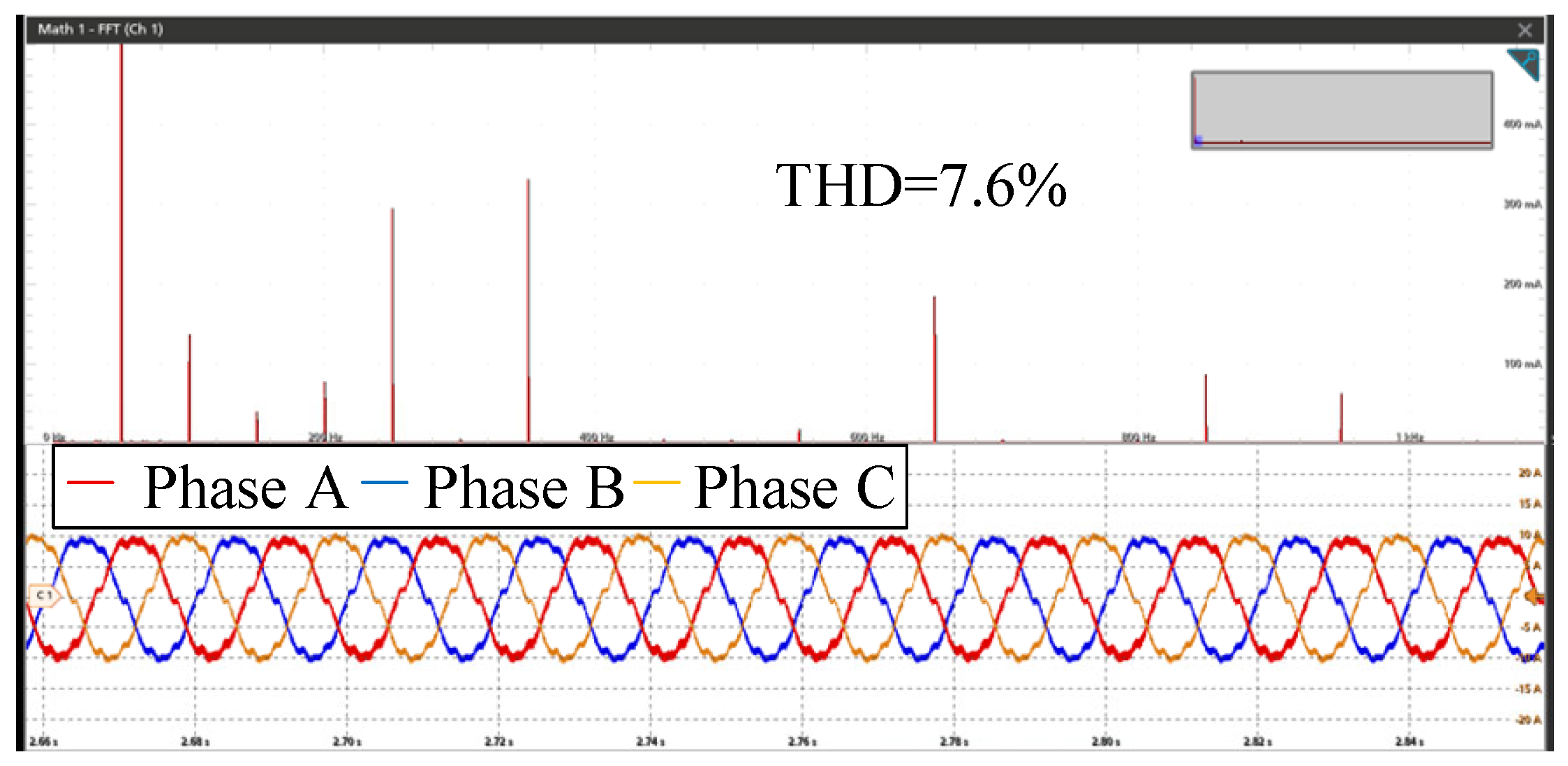
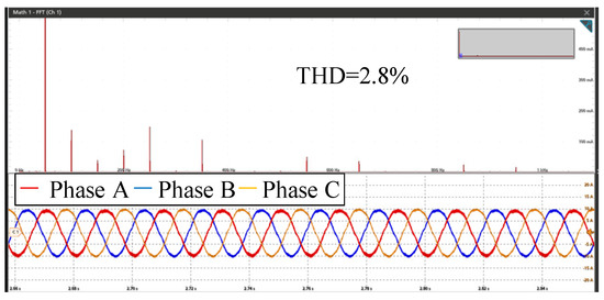
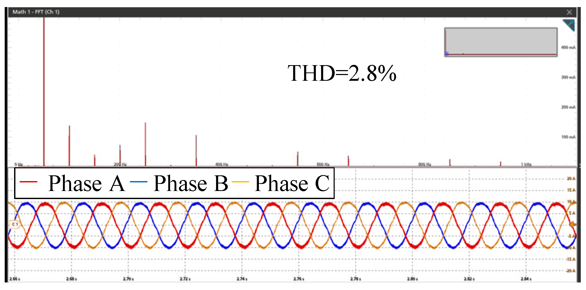
To verify the capability of the designed admittance-reshaping method to mitigate the influence of grid background harmonics, the 5th, 7th, 13th, 17th, and 19th harmonics were injected into the grid voltage, with harmonic contents of 4.5%, 3.5%, 2.5%, 1.5%, and 1%, respectively. After harmonic-disturbance voltages were injected, the converter output-current waveforms and the corresponding FFT results before and after applying the admittance-reshaping method are shown in Figure 23 and Figure 24, respectively.
Figure 23.
Grid-current information after harmonic injection without compensation.
Figure 24.
Grid-current information after harmonic injection with compensation.
As shown in Figure 23 and Figure 24, the grid current is severely distorted before the compensation method is applied. After the compensation method is adopted, the quality of the grid current is improved, which is consistent with the theoretical and simulation results. This demonstrates that the proposed compensation method can effectively eliminate coupled harmonic currents, reduce the influence of voltage background harmonics, and improve power quality.
4.2.2. Verification of Stability Improvement Effect
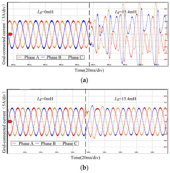
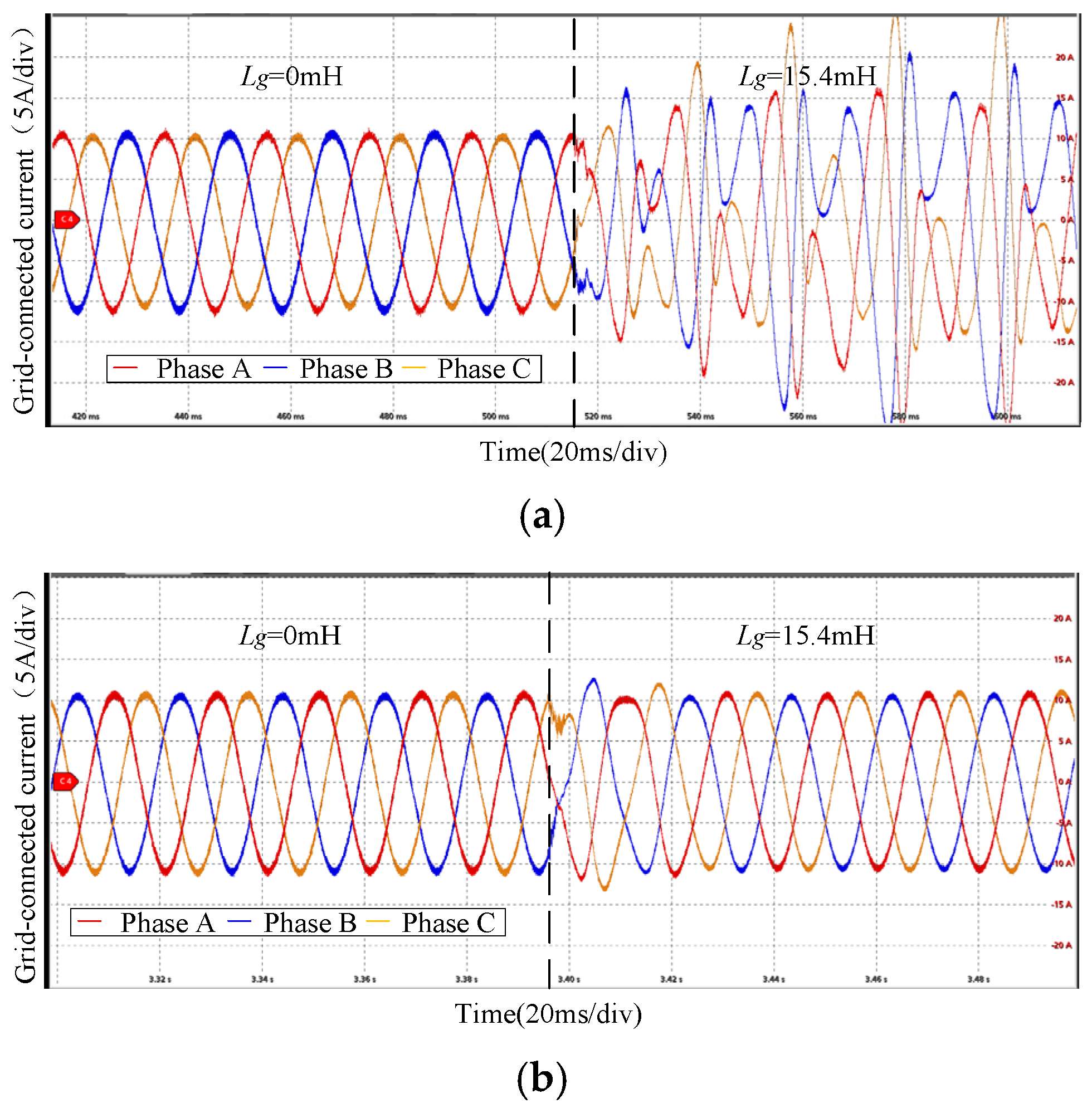
Figure 25 presents the experimental grid-connected current waveforms when the grid inductance increases from 0 mH to Lg = 15.4 mH (SCR = 3). It can be observed that the system operates from an ideal grid to a weak grid. Without compensation, the grid-connected current exhibits obvious instability. After applying the proposed compensation, the system can recover rapidly even under weak grid conditions. This further verifies the effectiveness of the presented method in improving the stability of grid-connected converters in weak grid scenarios.
Figure 25.
Experimental grid-current waveforms of the converter when Lg = 15.4 mH (SCR = 3): (a) before compensation; (b) after compensation.
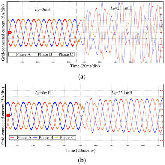
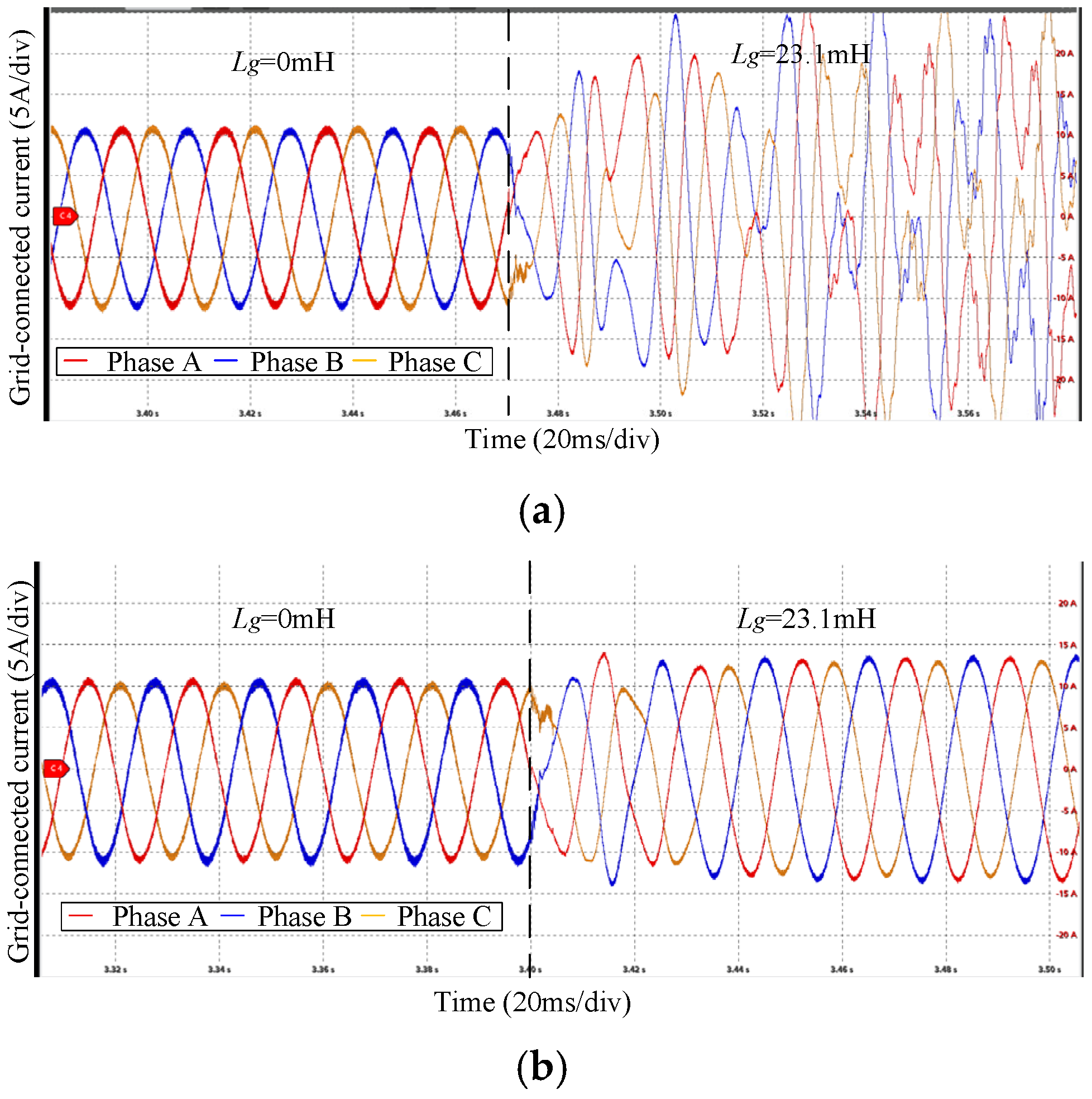
With other system parameters unchanged, the grid inductance is increased to Lg = 23.1 mH (SCR = 2). The experimental grid-connected current waveforms before and after compensation are shown in Figure 26. It can be seen that under this weak grid condition, the uncompensated grid-connected current suffers from obvious distortion and the system operates unstably. By contrast, the system remains stable when the grid inductance rises from 0 mH to 23.1 mH after adopting the compensation strategy.
Figure 26.
Experimental grid-current waveforms of the converter when Lg = 23.1 mH (SCR = 2): (a) before compensation; (b) after compensation.
4.2.3. Verification of System Dynamic Performance
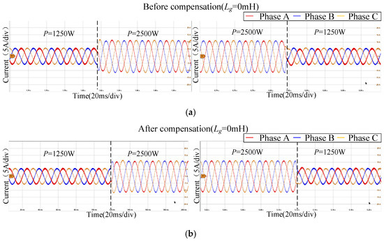
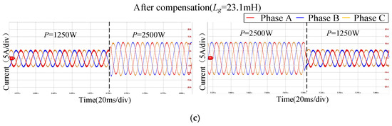
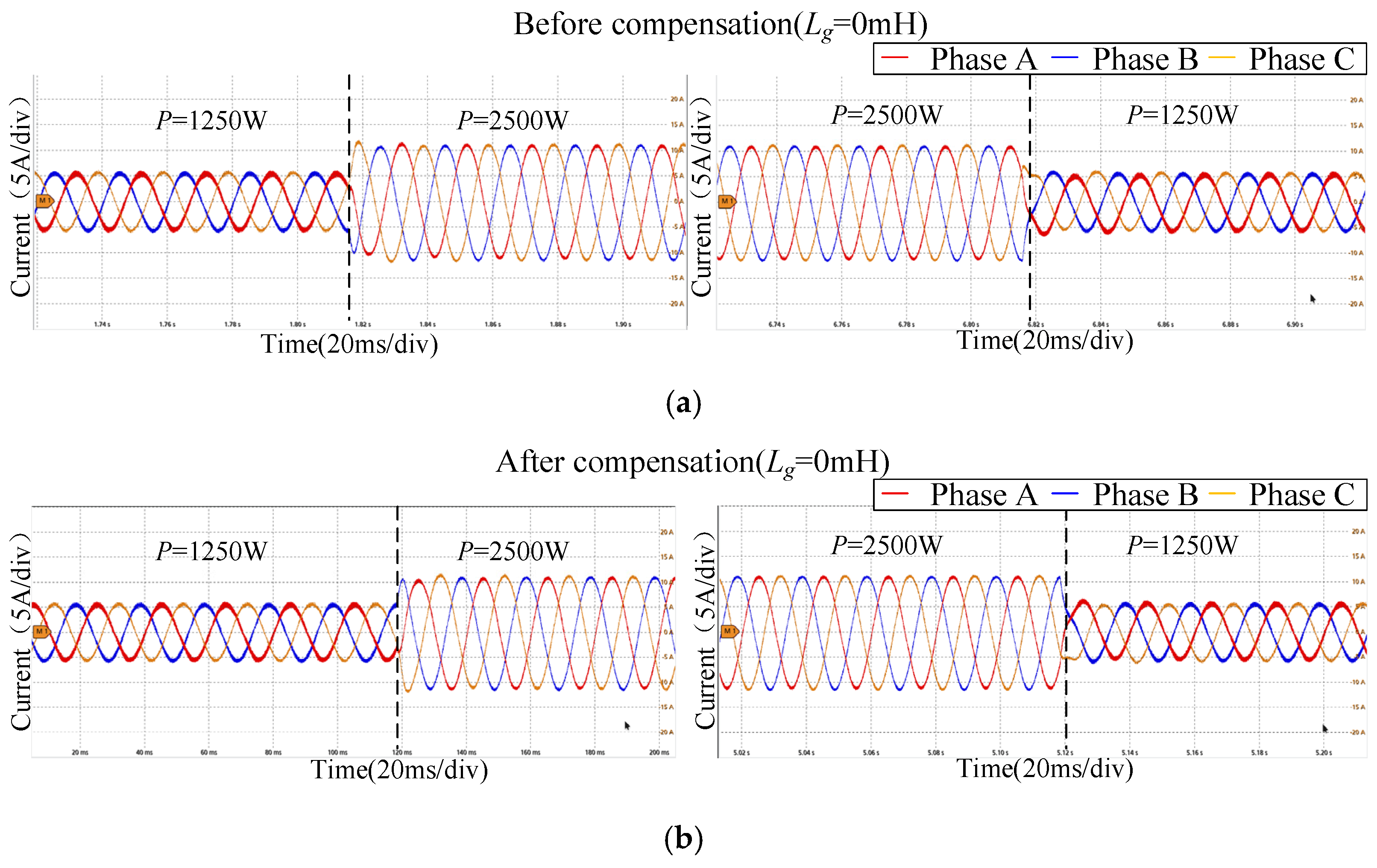
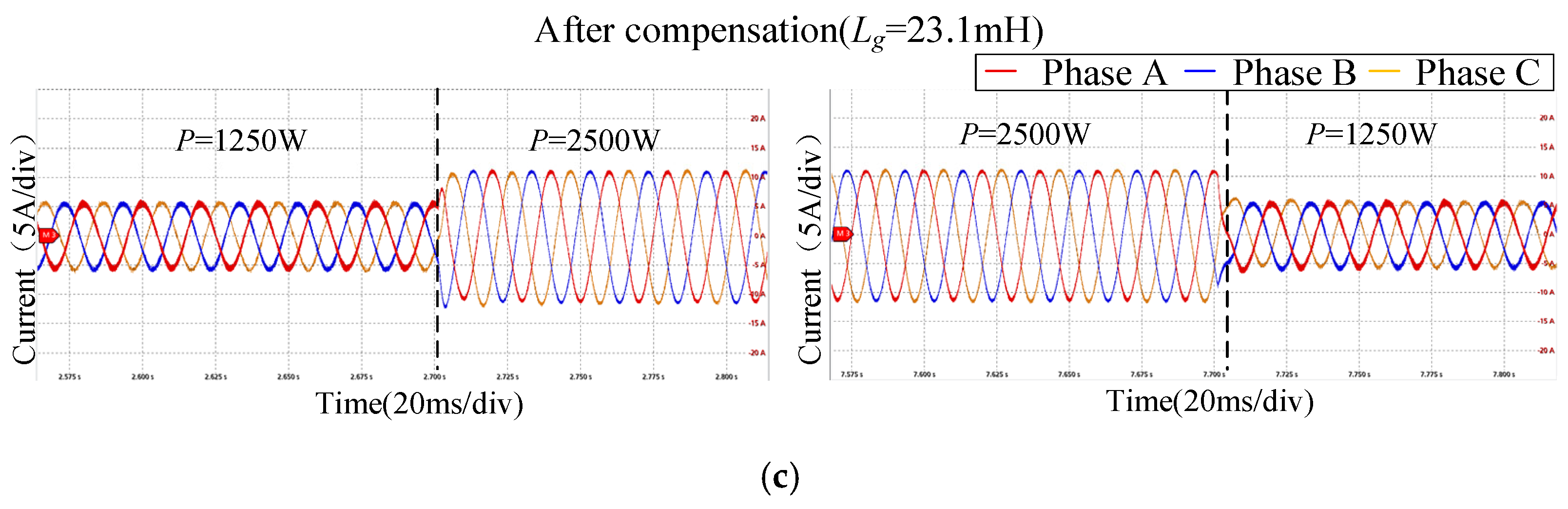
Figure 27 shows the grid-current waveforms under different grid-impedance conditions when the system switches from half load to full load and then back to half load before and after applying the proposed compensation. The experimental results in Figure 27 indicate that, both before and after compensation, when the DC-side input power increases from 1250 W to 2500 W and then decreases to 1250 W, the grid current can rapidly transition to the new operating point and maintain stable operation. This demonstrates that when the system operating point changes, the proposed compensation method has almost no effect on the dynamic response speed of the converter, and the system still exhibits good dynamic response performance.
Figure 27.
Experimental grid-current waveforms of the converter when the DC-side power Pin changes under different grid-impedance conditions: (a) before compensation (Lg = 0 mH); (b) after compensation (Lg = 0 mH); (c) after compensation (Lg = 23.1 mH).
5. Conclusions
This paper takes three-phase LCL-type grid-connected converters as the research object and establishes the output-admittance model of the system in the dq coordinate system. Aiming at the power quality and stability issues caused by background harmonics and weak grid conditions, an optimized control method based on admittance reshaping is proposed. The main conclusions are summarized as follows:
- (1)
- A decoupling compensation matrix is adopted to convert the two-input two-output-admittance model of the grid-connected converter into a single-input single-output form, which eliminates frequency coupling induced by asymmetric control structures. This method fundamentally removes mirror harmonics and achieves prominent suppression on typical background harmonics, thus improving the quality of grid-connected current. For stability problems under weak grid conditions, a compensation link is introduced into the feedforward path for phase correction, which increases the phase margin and enhances system stability.
- (2)
- Simulations and experiments are carried out on typical 5th, 7th, 13th, 17th and 19th order background harmonics covering the main broadband harmonic range in power systems. The results verify the excellent harmonic suppression capability of the proposed method. It can effectively eliminate mirror harmonic currents caused by background harmonics and improve power quality. Meanwhile, the system maintains satisfactory dynamic and stable performance under wide-range variations of grid impedance, which greatly enhances the adaptability of the converter to weak grids.
- (3)
- The proposed control strategy exhibits superior robustness under various complex operating conditions, including reasonable fluctuations of PLL bandwidth, current loop parameters and digital control delay, as well as wide grid impedance variation and unbalanced grid voltage. Compared with existing admittance-reshaping methods, the two schemes achieve similar harmonic suppression performance, while the proposed strategy possesses higher stability margin and better grid adaptability under weak and extremely weak grid conditions.
Author Contributions
Conceptualization, J.J. and X.T.; Methodology, J.J. and X.T.; Validation, J.J.; Formal analysis, J.J.; Resources, Z.Z., K.T. and J.W.; Writing—original draft, J.J.; Writing—review & editing, J.J., X.T., Z.Z., K.T. and J.W.; Supervision, Z.Z., K.T. and J.W. All authors have read and agreed to the published version of the manuscript.
Funding
This research received no external funding.
Data Availability Statement
No new data were created or analyzed in this study.
Conflicts of Interest
The authors declare no conflict of interest.
Appendix A
Since Δθ approaches 0, Equation (3) can be simplified as:
where
Substituting Equation (A1) yields:
After matrix rearrangement, Equation (4) can be obtained.
Equation (5) is derived by converting the KCL and KVL of the LCL circuit topology into the dq coordinate system and performing small-signal linearization. The derivation is presented taking the KVL between ucdq and usdq as an example.
The KVL in the three-phase stationary coordinate system is expressed as:
After performing Laplace transform on Equation (A4), the formula is converted to the dq coordinate system via Park transformation:
Small-signal linearization is implemented for Equation (A5). Each variable is decomposed into the steady-state component and small-signal perturbation component:
After eliminating the steady-state terms in Equation (A6) and reorganizing into matrix form, the first part of Equation (5) is obtained.
The derivation procedures for the relationships between Δigdq and ΔiL1dq, as well as Δugdq and Δucdq in Equation (5) follow the same rules. Thus we can obtain:
The upper part of Equation (6) is derived by substituting Equations (A8) and (A9) into Equation (A7). The lower part represents the expression of capacitor current.
where .
It can be derived from the active power balance between the AC and DC sides that:
Assuming that the q-axis voltage and current components are zero under steady state, the expression can be obtained after Laplace transform, small-signal linearization and matrix arrangement:
where .
Equation (8) is the small-signal expression of the control circuit, which is derived according to the control structure shown in the main circuit topology of Figure 1:
After matrix transformation, we can obtain:
The specific expressions for the elements of the output-admittance matrices Y(s), Y1(s) and Y2(s) of the grid-connected inverter are given as follows:
where
Figure A1.
FFT spectra of grid-connected current under different current loop bandwidths.
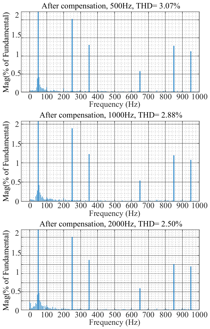
Figure A2.
FFT spectra of grid-connected current under different grid impedances.
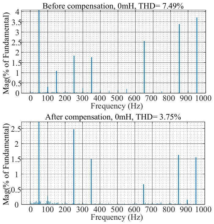
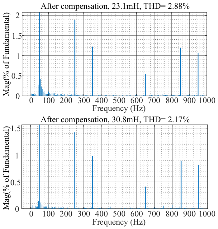
Figure A3.
FFT spectra of grid-connected current under different control delays.
Appendix B
Table A1.
The system parameters.
References
- Li, B.; Chen, M.; Zhong, H.; Ma, Z.; Liu, D. A Review of Long-term Planning of New Power Systems With Large Share of Renewable Energy. Proc. CSEE 2023, 43, 555–581. (In Chinese) [Google Scholar]
- Xin, B.; Shan, B.; Li, Q.; Yan, H.; Wang, C. Rethinking of the “three elements of energy” toward carbon peak and carbon neutrality. Proc. CSEE 2022, 42, 3117–3125. (In Chinese) [Google Scholar]
- Wang, J.; Liu, Q.; Han, W.; Xin, Z. Self-stabilizing Control Strategy for Grid-connected Inverters with Dynamic Performance-friendly Operation in Weak Grid. Proc. CSEE 2026, 46, 1154–1164. (In Chinese) [Google Scholar]
- Zhang, Q.; Cai, F.; Huang, L.; Chen, X. PI+ repetitive control applied to single-phase programmable standard power source. Trans. China Electrotech. Soc. 2019, 34, 163–170. (In Chinese) [Google Scholar]
- Liu, X.; Jiang, W.; Li, Y. Second harmonic transmission mechanism and suppression measures in Qinghai power grid. Power Syst. Technol. 2015, 39, 2277–2282. (In Chinese) [Google Scholar]
- Zhou, P.; Xiang, Z.; Du, N.; Ban, L.; Xie, G. Analysis on blocking of Qinghai-Tibet DC system caused by transformer energizing in Northwest China 750 kV grid. Autom. Electr. Power Syst. 2013, 37, 129–133. (In Chinese) [Google Scholar]
- Xie, X.; Liu, H.; He, J.; Zhang, C.; Qiao, Y. Mechanism and characteristics of sub-synchronous oscillation caused by the interaction between full-converter wind turbines and AC systems. Proc. CSEE 2016, 36, 2366–2372. (In Chinese) [Google Scholar]
- Ma, J.; Zhao, D.; Qian, M.; Zhu, L.; Yao, L.; Wang, N. Reviews of control technologies of large-scale renewable energy connected to weakly-synchronized sending-end DC power grid. Power Syst. Technol. 2017, 41, 3112–3120. (In Chinese) [Google Scholar]
- Zhang, D.; Chen, X. Overview of Broadband Oscillation Mitigation of New Energy Generation Power System Based on Impedance Perspective. Proc. CSEE 2024, 44, 9672–9691. (In Chinese) [Google Scholar]
- Nian, H.; Xu, Y.; Chen, L.; Li, G. Frequency coupling characteristic modeling of grid-connected inverter and system stability analysis. Proc. CSEE 2019, 39, 1421–1431. (In Chinese) [Google Scholar]
- Yang, D.; Wang, X.; Liu, F.; Xin, K.; Liu, Y.; Blaabjerg, F. Symmetrical PLL for SISO impedance modeling and enhanced stability in weak grids. IEEE Trans. Power Electron. 2020, 35, 1473–1483. [Google Scholar] [CrossRef] [Scilit]
- Nian, H.; Hu, B.; Xu, Y.; Wu, C.; Chen, L.; Blaabjerg, F. Analysis and reshaping on impedance characteristic of DFIG system based on symmetrical PLL. IEEE Trans. Power Electron. 2020, 35, 11720–11730. [Google Scholar] [CrossRef] [Scilit]
- Wang, X.; Yang, A.; Liu, Y.; Zhao, X. Stability control study of grid-connected inverters considering frequency coupling effect. Power Syst. Technol. 2023, 47, 3280–3295. (In Chinese) [Google Scholar]
- Wang, X.; Ruan, X.; Liu, S.; Tse, C.K. Full feedforward of grid voltage for grid-connected inverter with LCL filter to suppress current distortion due to grid voltage harmonics. IEEE Trans. Power Electron. 2010, 25, 3119–3127. [Google Scholar] [CrossRef] [Scilit]
- Yang, D.; Ruan, X.; Wu, H. Impedance shaping of the grid-connected inverter with LCL filter to improve its adaptability to the weak grid condition. IEEE Trans. Power Electron. 2014, 29, 5795–5805. [Google Scholar] [CrossRef] [Scilit]
- Yang, D.; Ruan, X.; Wu, H. A real-time computation method with dual sampling mode to improve the current control performance of the LCL-type grid-connected inverter. IEEE Trans. Ind. Electron. 2015, 62, 4563–4572. [Google Scholar] [CrossRef] [Scilit]
- Ling, Y.; Zeng, J.; Liu, Y.; Yang, L. Virtual-resistance-type photovoltaic inverter with low-order harmonics suppression. Autom. Electr. Power Syst. 2018, 42, 114–119. (In Chinese) [Google Scholar] [CrossRef] [Scilit]
- Wang, F.; Duarte, J.L.; Hendrix, M.A.; Ribeiro, P.F. Modeling and analysis of grid harmonic distortion impact of aggregated DG inverters. IEEE Trans. Power Electron. 2010, 26, 786–797. [Google Scholar] [CrossRef] [Scilit]
- Jia, Y.; Zhao, J.; Fu, X. Direct grid current control of LCL-filtered grid-connected inverter mitigating grid voltage disturbance. IEEE Trans. Power Electron. 2013, 29, 1532–1541. [Google Scholar]
- Liserre, M.; Teodorescu, R.; Blaabjerg, F. Multiple harmonics control for three-phase grid converter systems with the use of PI-RES current controller in a rotating frame. IEEE Trans. Power Electron. 2006, 21, 836–841. [Google Scholar] [CrossRef] [Scilit]
- Lin, Z.; Ruan, X.; Wu, L.; Zhang, H.; Li, W. Multi resonant component-based grid-voltage-weighted feedforward scheme for grid-connected inverter to suppress the injected grid current harmonics under weak grid. IEEE Trans. Power Electron. 2020, 35, 9784–9793. [Google Scholar] [CrossRef] [Scilit]
- Yan, P.; Ge, X.; Wang, H.; Sun, W.; Zhu, Y. PLL Parameter Optimization Design for Renewable Energy Grid-connected Inverters in Weak Grid. Power Syst. Technol. 2022, 46, 2210–2221. (In Chinese) [Google Scholar]
- Ravanji, M.H.; Rathnayake, D.B.; Mansour, M.Z.; Bahrani, B. Impact of voltage-loop feedforward terms on the stability of grid-forming inverters and remedial actions. IEEE Trans. Energy Convers. 2023, 38, 1554–1565. [Google Scholar] [CrossRef] [Scilit]
- Tang, X.; He, Y.; Li, Z.; Li, X. Frequency Division Compensation Method for Phase Margin of Grid Connected Converters in the Weak Grid. Proc. CSEE 2024, 44, 1565–1576. (In Chinese) [Google Scholar]
- Yang, S. Research on Stability and Oscillation Suppression Strategy of HVDC Transmission System with Series Compensation. Master’s Thesis, Chongqing University, Chongqing, China, 2022. [Google Scholar]
- Tang, X.; Li, Z.; Wang, W.; Liu, L.; Qu, B.; Guerrero, J.M. A decoupling control method for converting DIDO sequence admittance model of grid-tied converter system into SISO. IEEE Trans. Energy Convers. 2023, 38, 2647–2661. [Google Scholar] [CrossRef] [Scilit]
- Li, Z.; Tang, X.; He, Y.; Liu, P.; Li, X. Admittance Reshaping Method of Converter for Suppressing Background Harmonic of Grid. Proc. CSEE 2024, 44, 704–714. (In Chinese) [Google Scholar]
- Wang, K.; Yuan, X.; Wang, H.; Zhang, Y.; Wu, X. Two Causes of the Inverter-based Grid-connected System Instability in Weak Grids. Power Syst. Technol. 2023, 47, 1230–1242. (In Chinese) [Google Scholar]
- Yang, M.; Li, Y.; Yang, Z.; Zhu, J.; Xie, B. High Robust Stability Control Strategy of Grid-connected Inverter Based on Capacitor Voltage Full Feedforward. High Volt. Eng. 2024, 50, 4171–4183. [Google Scholar]
- Akhavan, A.; Mohammadi, H.R.; Vasquez, J.C.; Guerrero, J.M. Passivity-based design of plug-and-play current-controlled grid-connected inverters. IEEE Trans. Power Electron. 2020, 35, 2135–2150. [Google Scholar] [CrossRef] [Scilit]
- Zhang, L.; Wang, F.; Feng, X. Control-loop optimizations based on output-impedance enhancement for disturbance suppression of grid voltage. Proc. CSEE 2018, 38, 1177–1186+1295. (In Chinese) [Google Scholar]
- Rygg, A.; Molinas, M.; Zhang, C.; Cai, X. A Modified Sequence-Domain Impedance Definition and Its Equivalence to the dq-Domain Impedance Definition for the Stability Analysis of AC Power Electronic Systems. IEEE J. Emerg. Sel. Top. Power Electron. 2016, 4, 1383–1396. [Google Scholar] [CrossRef] [Scilit]
Disclaimer/Publisher’s Note: The statements, opinions and data contained in all publications are solely those of the individual author(s) and contributor(s) and not of MDPI and/or the editor(s). MDPI and/or the editor(s) disclaim responsibility for any injury to people or property resulting from any ideas, methods, instructions or products referred to in the content. |
© 2026 by the authors. Licensee MDPI, Basel, Switzerland. This article is an open access article distributed under the terms and conditions of the Creative Commons Attribution (CC BY) license.