Partial Discharge Signal Denoising for Gas-Insulated Switchgear Using Spearman Coefficient-Optimized VMD and Combined Filtering Algorithm

Abstract

Partial discharge (PD) signals acquired from gas-insulated switchgear (GIS) are often severely contaminated by discrete-spectrum interference and periodic narrowband noise, which impairs the accuracy of subsequent fault diagnosis. This paper proposes a hybrid denoising method that integrates Spearman coefficient-optimized variational mode decomposition (S_VMD), spatially related recursive sample entropy (Sdr_SampEn) for intrinsic mode function (IMF) classification, an improved wavelet threshold function, and Savitzky–Golay (SG) filtering. First, the Spearman correlation coefficient between the original signal and the reconstructed signal is used to adaptively determine the optimal mode number K of VMD, avoiding the over- and under-decomposition problems of conventional VMD. Second, Sdr_SampEn, which characterizes signal irregularity along both the Chebyshev distance and spatial direction of a recurrence plot, is employed to classify the obtained IMFs into noise-dominant and PD-dominant components, with the discrimination threshold calibrated as p = 1.94 at 0 dB. Third, an improved wavelet threshold function—continuous at the threshold and asymptotically unbiased—is applied to the noise-dominant components, while SG filtering is applied to the PD-dominant components, after which the denoised signal is reconstructed. The results demonstrate that the proposed method effectively suppresses both white and narrowband noise while preserving the detailed morphology of PD pulses.

1. Introduction

Gas-insulated switchgear (GIS) is a key component of modern high-voltage and extra-high-voltage power transmission systems, and its operating reliability is critical to grid safety. Insulation defects introduced during manufacture, assembly or long-term operation—such as surface scratches, attached metallic particles and protrusions—can trigger partial discharge (PD), which progressively degrades the solid insulation and may ultimately lead to catastrophic flashover [1]. Online PD monitoring is therefore widely regarded as one of the most effective means of assessing the insulation condition of GIS [2].

In practice, however, the PD pulses captured by ultra-high-frequency (UHF) or high-frequency current transformer (HFCT) sensors are typically buried in strong background noise, which can be categorized into two groups: (i) white Gaussian noise originating from the sensor front-end and the data-acquisition system, and (ii) periodic narrowband interference from high-order harmonics, communication carriers and coupled radio signals [3]. Effective denoising is thus a prerequisite for any downstream task such as PD source localization, pattern recognition, or severity assessment.

Existing denoising techniques for PD signals can be broadly grouped into three categories. (1) Wavelet-based methods decompose the signal into multi-scale coefficients and apply hard or soft thresholding. Although widely used, the hard threshold introduces discontinuities that cause oscillations in the reconstructed signal, while the soft threshold produces a fixed bias that distorts pulse amplitude [4]. (2) Mode-decomposition methods such as empirical mode decomposition (EMD), complementary ensemble EMD (CEEMD), CEEMDAN, and variational mode decomposition (VMD) decompose non-stationary signals into a set of intrinsic mode functions (IMFs). Among these, VMD has a solid variational foundation and is free from mode mixing, but its performance is highly sensitive to the preset mode number K and penalty factor α [5]. (3) Hybrid and learning-based methods such as SVD-VMD and PRPD-based filtering combine multiple techniques but often lack an adaptive, data-driven rule for distinguishing PD-dominant from noise-dominant components [6,7,8].

Furthermore, in recent years, artificial intelligence (AI) and deep learning-based approaches have emerged as highly popular tools for PD noise suppression. Researchers have extensively explored techniques such as Denoising Autoencoders (DAE), Convolutional Neural Networks (CNNs), and Recurrent Neural Networks (RNNs) to automatically extract PD features from heavy background noise [9,10,11]. These data-driven methods exhibit remarkable denoising performance and do not require manual threshold tuning. However, despite their immense potential, purely AI-based methods face several practical challenges in real-world GIS engineering. First, they typically require massive, high-quality labeled datasets for training, which are exceptionally difficult to acquire in actual substations. Second, due to their “black-box” nature, these models often lack physical interpretability. Finally, AI models can suffer from severe generalization degradation when encountering unseen, complex noise distributions in a new operating environment.

Motivated by these limitations, this paper proposes an adaptive hybrid denoising framework for GIS PD signals. The main contributions are threefold: (1) An adaptive VMD scheme (S_VMD) is proposed, in which the optimal mode number K is determined online from the Spearman correlation coefficient between the original and the reconstructed signals, eliminating the need for manual tuning [12]. (2) A spatially related recursive sample entropy (Sdr_SampEn) indicator is introduced to classify the obtained IMFs into noise-dominant and PD-dominant components along both the Chebyshev distance and the spatial direction of a recurrence plot, with the discrimination threshold quantitatively calibrated [13]. (3) An improved wavelet threshold function that is continuous at the threshold and asymptotically approaches the identity mapping is combined with SG filtering to process noise-dominant and PD-dominant components separately, achieving an effective trade-off between noise suppression and pulse-shape preservation [14,15].

2. Materials and Methods

2.1. Variational Mode Decomposition

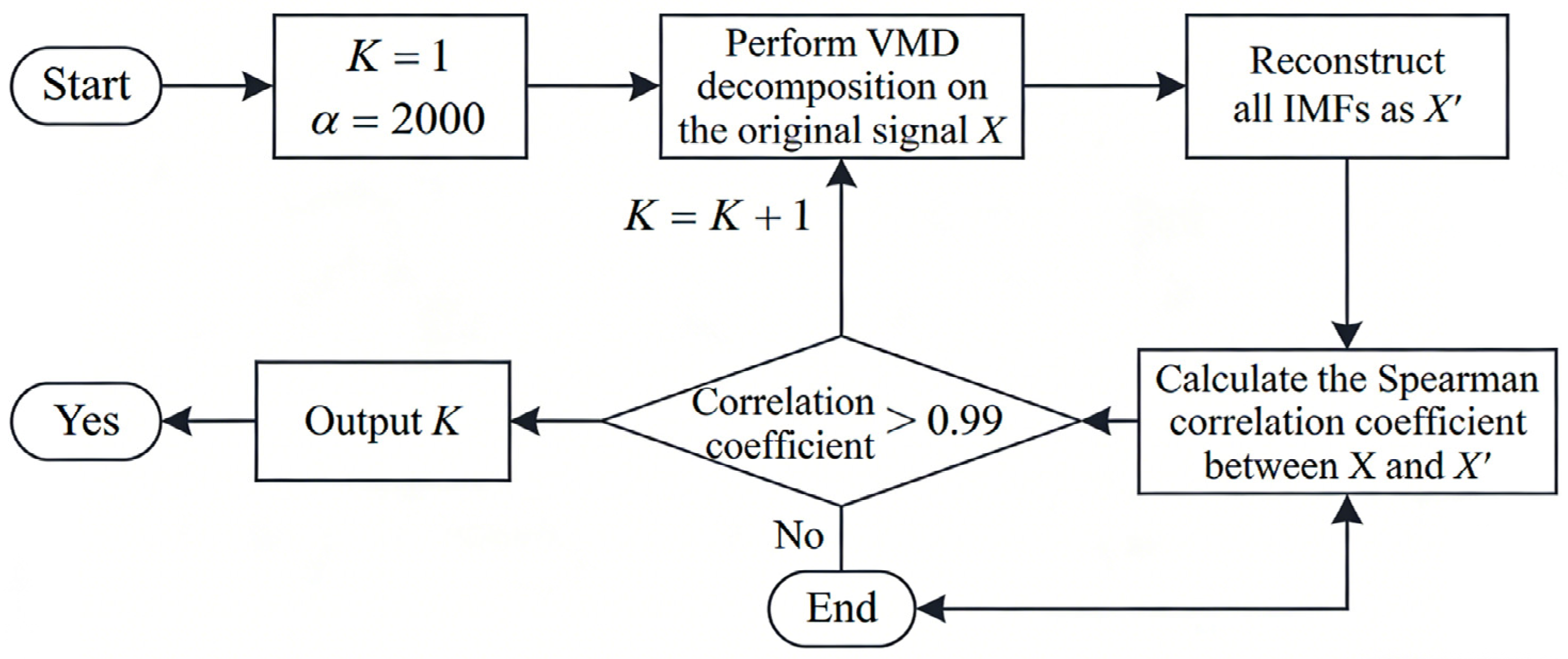
VMD is a kind of adaptive, non-recursive signal processing method, particularly effective for nonlinear non-stationary signals. The core of the VMD algorithm lies in variational solving, which continuously iterates to determine the center frequency and bandwidth of each intrinsic mode function (IMF), decomposing the signal into K components while minimizing the sum of the estimated bandwidths of each IMF. The parameters K and α in the algorithm are crucial; K determines the number of IMFs the algorithm extracts, while α determines the rate of decay of the IMF’s frequency bands. When α is too large, the decomposition rate is too fast, leading to excessive removal of the effective portions between adjacent IMFs; when α is too small, noticeable band overlap occurs. Literature [16] indicates that when α is set to 2000, the adaptive effect is optimal, yielding the best denoising results [16]. For the parameter K, this paper employs the Spearman correlation coefficient to determine its optimal value [17].

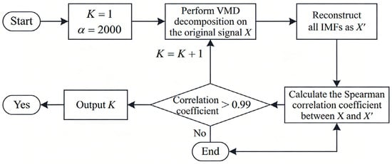
The original signal X can be decomposed into K IMFs by the VMD algorithm. By reconstructing all IMFs into X′, from the definition of the Spearman correlation coefficient, it is evident that as the parameter K increases, the Spearman correlation coefficient between X and X′ shows an increasing trend. After X is completely decomposed, with the increase in K, there will be multiple IMFs with very similar central frequencies, which indicates over-decomposition. To avoid the aforementioned phenomenon, this paper conducted a large number of simulation experiments, and the results show that when the correlation coefficient reaches 0.99, the signal has been completely decomposed. In summary, the process for determining the optimal parameter K is shown in Figure 1.

Figure 1. Process of determining the optimal parameter K.

2.2. Spatially Related Recursive Sample Entropy

Following the decomposition of the signal into IMFs via VMD, a robust quantitative criterion is indispensable to distinguish noise-dominant components from those containing meaningful PD information. Although conventional sample entropy is widely used, it evaluates only temporal irregularity; consequently, it fails when narrowband periodic interference exhibits amplitude statistics similar to genuine PD pulses. To address this limitation, this study employs Sdr_SampEn [13]. This metric jointly quantifies signal complexity across two complementary dimensions: the Chebyshev distance within the reconstructed phase space and the spatial co-occurrence structure of the recurrence plot.

Let a set of sequence information be $X=\{x_1,x_2,x_3,\cdots ,x_N\}$ and obtain the corresponding reconstructed phase space by applying coordinate delay, as shown in Equation (1).

$$X_i=\left\{x_i,x_{i+\tau },{\cdots ,x}_{i+(m-1)\tau },\right\}$$

(1)

where $X_i$ denotes the vector in the reconstructed phase space; $i=\mathrm{1,2},\cdots ,N-\left(m-1\right)\tau$ represents the time delay; and $m$ stands for the embedding dimension.

The recursive matrix for constructing the phase space is illustrated in Equation (2).

$$R_{i,j}=\Theta \left(\epsilon -d\left(X_i,X_j\right)\right)=\{\begin{array}{c}1,\epsilon \ge d\left(X_i,X_j\right)\\ 0,\epsilon <d\left(X_i,X_j\right)\end{array}$$

(2)

where $d\left(X_i,X_j\right)$ denotes the Chebyshev distance between $X_i$ and $X_j$; $\Theta \left(·\right)$ represents the Heaviside function; and $\epsilon$ stands for the fixed recurrence threshold.

By substituting any two vectors from the reconstructed space into the above formula, one can obtain an $N\times N$ matrix. If the value at the $(i,j)$ coordinates is represented by a black dot, then a recursive graph of a time series reconstructed in phase space can be obtained.

By defining $\delta =({\delta }_x,{\delta }_y)$ and conceptualizing the recurrence plot as a binary image populated by black (recurrent) and white (non-recurrent) pixels, spatial attributes can be effectively incorporated. A BLCM is subsequently formulated through the pixel-scanning process regulated by a predefined spatial offset, borrowing from the framework of gray-level co-occurrence matrices. Consequently, as defined in Equation (3), the individual matrix element $BLCM(p,q)$ quantifies the occurrences of adjacent pixel pairs that possess the respective binary states of $p$ and $q$.

$$B_{\mathsf{\delta }}\left(p,q\right)=\sum _{x=1}^N\sum _{y=1}^N\left[I\left(x,y\right)=p\right]\wedge \left[I\left(x+{\delta }_x,y+{\delta }_y\right)=q\right]$$

(3)

where $I(x,y)$ and $I\left(x+{\delta }_x,y+{\delta }_y\right)$ denote the pixel values at positions $\left(x,y\right)$ and $\left(x+{\delta }_x,y+{\delta }_y\right)$, respectively; $p,q\in$ {0,1} denote the possible binary pixel values; and $\wedge$ represents the logical “AND” operation.

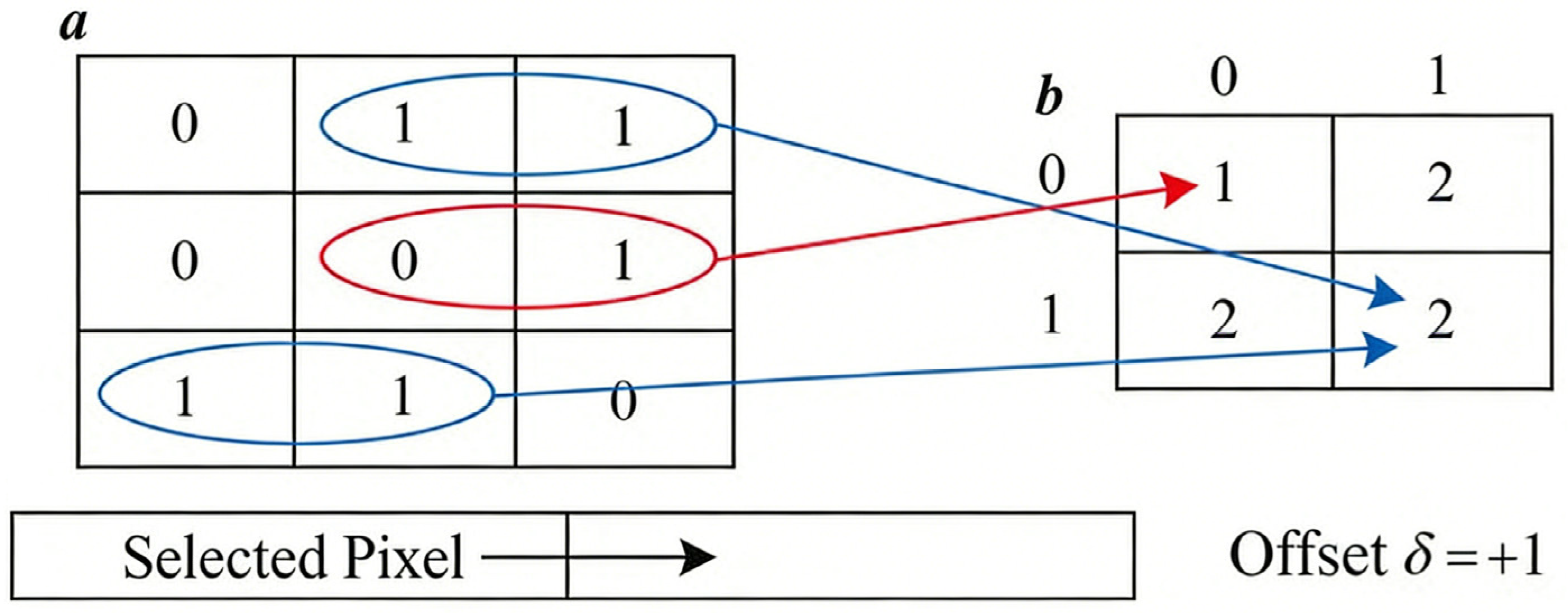
In this framework, the BLCM is established to systematically quantify the spatial distribution of the binary fields. Specifically, the diagonal elements $BLCM\left(\mathrm{0,0}\right)$ and $BLCM\left(\mathrm{1,1}\right)$ enumerate the co-occurrence frequencies of white (non-recurrent) and black (recurrent) pixel pairs, respectively, under a specified spatial displacement $∆=(d_x,d_y)$. To illustrate this positioning mechanism, let A denote the binary recurrence image, and let P represent its corresponding $BLCM$ derived using an offset of P. This distinct parameter configuration mandates that the target reference pixel is strictly positioned one unit horizontally to the right of the anchor pixel, as diagrammed in Figure 2.

Figure 2. Construction example of $BLCM$: (a) a $3\times 3$ binary recurrence matrix with highlighted horizontal pixel transitions; (b) the corresponding $BLCM$ under a horizontal offset of $\delta =+1$, enumerating the total frequencies of adjacent pixel pairs.

Based on the spatial orientation, sample similarity is quantified by translating the recurrence plot into a binary image to yield its corresponding $BLCM$. Under the constraint of a predefined spatial displacement $∆$ and $a$ Chebyshev distance threshold bounded below $r$, the aggregate probability of finding $m$-dimensional recurrent pixel pairs is formulated via Equation (4).

$$S^m\left(\mathsf{\epsilon },\mathsf{\delta }\right)={\displaystyle \frac{\mathrm{BLCM}\left(\mathrm{1,1}\right)}{N\left(\mathsf{\delta }\right)}}$$

(4)

where $BLCM\left(\mathrm{1,1}\right)$ denotes the total number of recurrence state pairs in the phase space reconstructed from the time series; $N\left(\delta \right)$ represents the total number of valid pixel pairs under the condition of offset $\delta$.

To summarize, the Sdr_SampEn approach provides a robust framework for characterizing the irregularity of time series, evaluated simultaneously under the criteria of Chebyshev distance metrics and spatial orientation configurations, as explicitly formulated in Equation (5).

$$\mathrm{Sdr}\text{\_}\mathrm{SampEn}\left(m,\mathsf{\epsilon },\mathsf{\delta }\right)=-\ln \left[{\displaystyle \frac{S^{m+1}\left(\mathsf{\epsilon },\mathsf{\delta }\right)}{S^m\left(\mathsf{\epsilon },\mathsf{\delta }\right)}}\right]$$

(5)

where $S^{m+1}(\epsilon ,\delta )\le S^m(\epsilon ,\delta )$.

The detailed computational procedure for evaluating the Sdr_SampEn metric is structured as follows:

• Define the target time series $X=\left\{x_1,x_2,x_3,{\cdots ,x}_N,\right\}$ and initialize the foundational model hyper-parameters, including the embedding dimension $m$, the tolerance threshold $r$, and the prescribed spatial displacement vector $∆$;
• Reconstruct the trajectory in the phase space and generate the corresponding recurence plot (RP) based on the Chebyshev distance metric;
• Construct the $BLCM$ by systematically scanning the generated RP to yield the joint probability matrix P;
• Quantify the spatial co-occurrence probabilities of the reconstructed states to determine the total match numbers (or local joint probabilities) for both $m$ and $m+1$ dimensions, denoted as $A^m(r,∆)$ and $B^m(r,∆)$;
• Compute the final Sdr_SampEn value by evaluating the negative natural logarithm of the conditional probability, as formulated in Equation (5).

2.3. Improved Wavelet Threshold Denoising and Savitzky–Golay Filtering

For noise-dominant components, this paper adopts a wavelet thresholding denoising method for processing. The idea of wavelet transform is to perform a wavelet transform on the noisy signal, obtaining a set of wavelet coefficients, then selecting an appropriate threshold to carry out corresponding filtering transformations on each layer of wavelet coefficients, and finally reconstructing the signal from the processed wavelet coefficients. Throughout the wavelet transform process, the determination of the wavelet threshold and the selection of the threshold function have a significant impact on the final denoising effect. This paper proposes a novel wavelet thresholding denoising method, with the threshold function shown in Equation (6).

$${\mathsf{\omega }}_{j,k}^{\prime }=\{\begin{array}{cc}\mathrm{sign}\left({\mathsf{\omega }}_{j,k}\right)\left(\left|{\mathsf{\omega }}_{j,k}\right|-{\displaystyle \frac{\mathsf{\lambda }}{{\mathrm{e}}^{\left|{\mathsf{\omega }}_{j,k}\right|-\mathsf{\lambda }}}}\right),& \left|{\mathsf{\omega }}_{j,k}\right|\ge \mathsf{\lambda }\\ 0,& \left|{\mathsf{\omega }}_{j,k}\right|<\mathsf{\lambda }\end{array}$$

(6)

where ${\omega }_{j,k}^{\prime }$ denotes the processed wavelet coefficients; ${\omega }_{j,k}$ represents the wavelet coefficients to be processed; $\lambda ={\displaystyle \frac{\sigma \sqrt{2\ln N}}{\ln (i+1)}}$ is the new wavelet threshold, where $N$ is the number of sampling points, $i$ is the decomposition level of the wavelet transform, and $\sigma$ is the standard deviation of the signal.

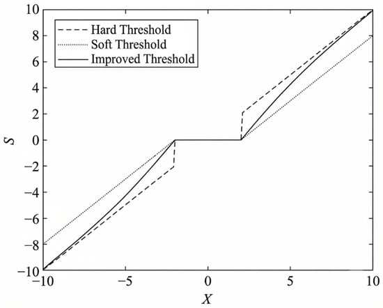
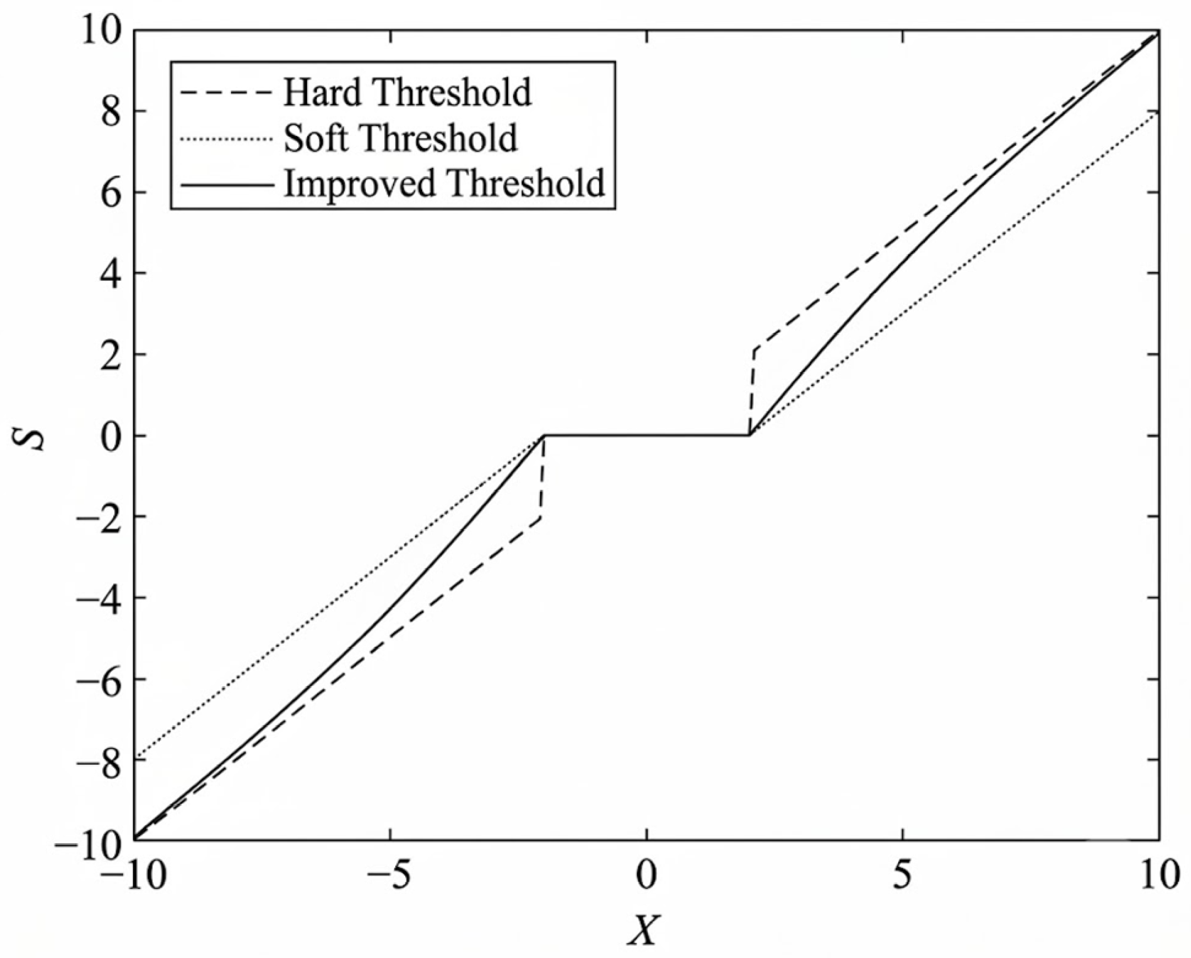
In order to highlight the characteristics of the new threshold function, a comparison is made between the new threshold function and the soft and hard threshold functions, taking $\sigma =1$, as shown in Figure 3.

Figure 3. Comparison of soft and hard threshold function and improved threshold function.

As shown in Figure 3, after processing with the hard threshold function, discontinuities appear at ${\omega }_{j,k}=\pm 1$, resulting in the denoised signal generating new oscillations. After processing with the soft threshold function, although the signal is continuous at ${\omega }_{j,k}=\pm 1$, there is a significant fixed difference between the processed signal and the original signal, leading to some distortion. The threshold function proposed in this paper is continuous at ${\omega }_{j,k}=\pm 1$, and as ${\omega }_{j,k}$ increases, the deviation between ${\omega }_{j,k}$ and ${\omega }_{j,k}^{\prime }$ continuously shrinks, overcoming the respective shortcomings of the soft and hard threshold functions.

For the PD-dominant component, this paper employs Savitzky–Golay (SG) filtering for denoising. SG filtering, also known as polynomial smoothing filtering based on the least squares principle, is a type of time-domain filtering. This method is widely used for the smooth denoising of data streams and can filter out noise while preserving the integrity of the signal shape. The specific approach involves first selecting a sliding window, followed by fitting the data with a univariate polynomial of a specified order, with the coefficients determined based on the least squares criterion. Finally, the window slides along the best-fit values to achieve the denoising effect.

2.4. The Denoising Method in This Article

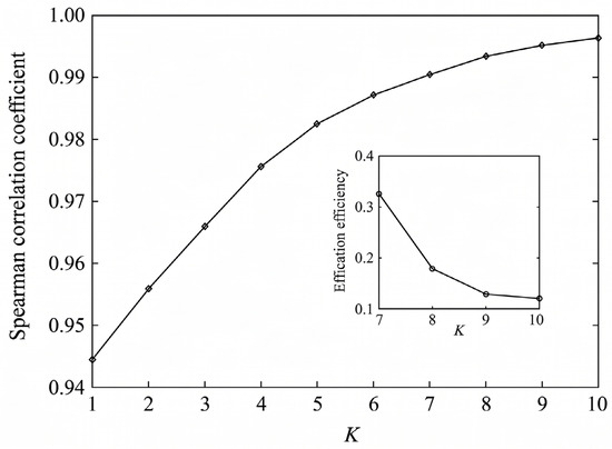
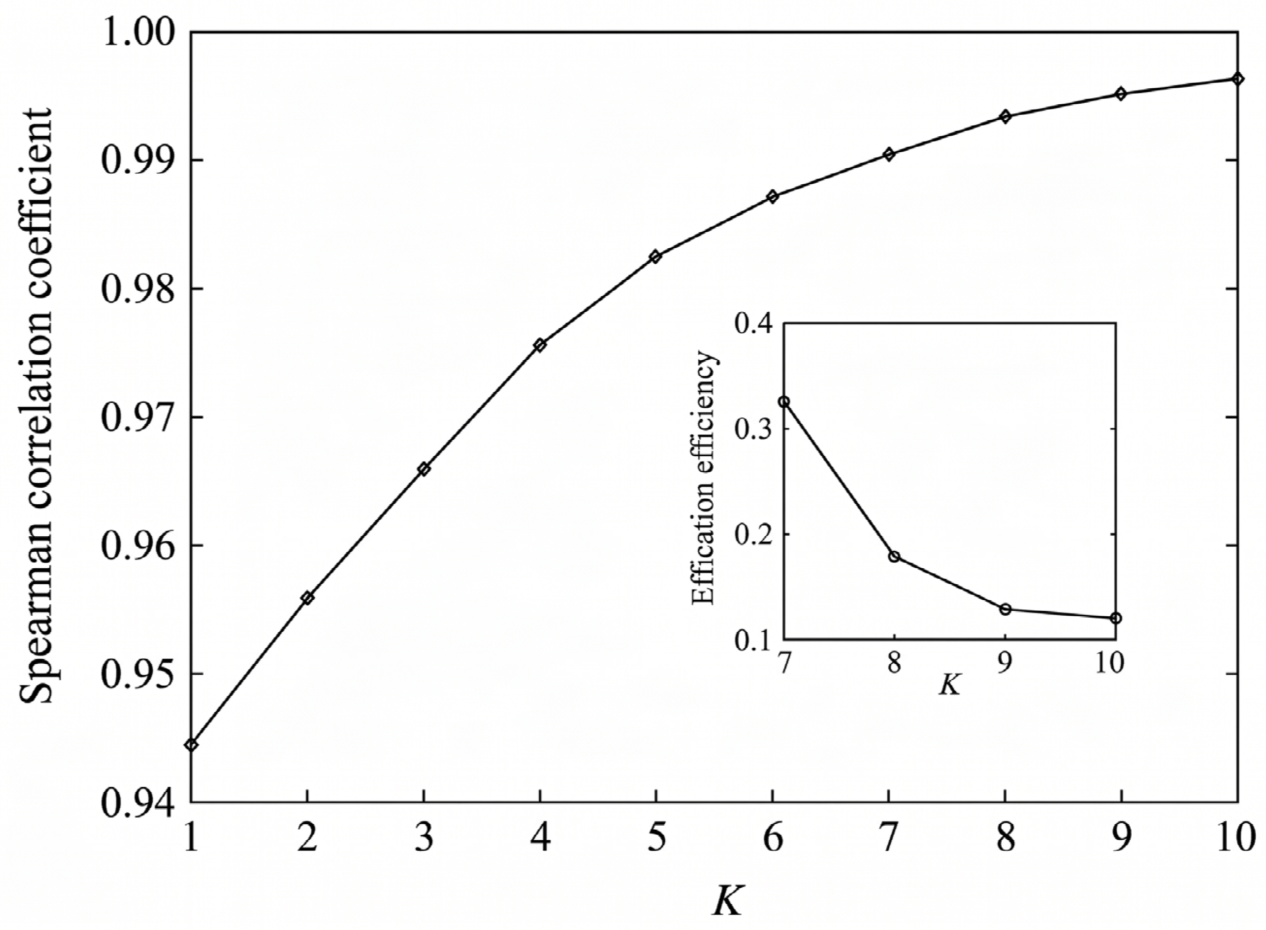
From the above principle, it can be seen that two key parameters need to be determined in this article: one is the K optimized by the Spearman correlation coefficient in VMD algorithm, and the other is the threshold p used in Sdr_SampEn algorithm to distinguish between noise-dominant components and PD-dominant components. For parameter K, after conducting a large number of simulation experiments, the relationship between K value and Spearman correlation coefficient can be obtained. According to Figure 4, when K = 7, the Spearman correlation coefficient has reached 0.99, but another part in Figure 4 clearly shows that as the value of K gradually increases from 7 to 10, the execution efficiency of the algorithm shows a significant downward trend (from 0.3 to about 0.1), indicating that K = 7 is the optimal solution.

Figure 4. Relationship between Spearman correlation coefficient and K.

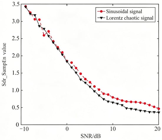
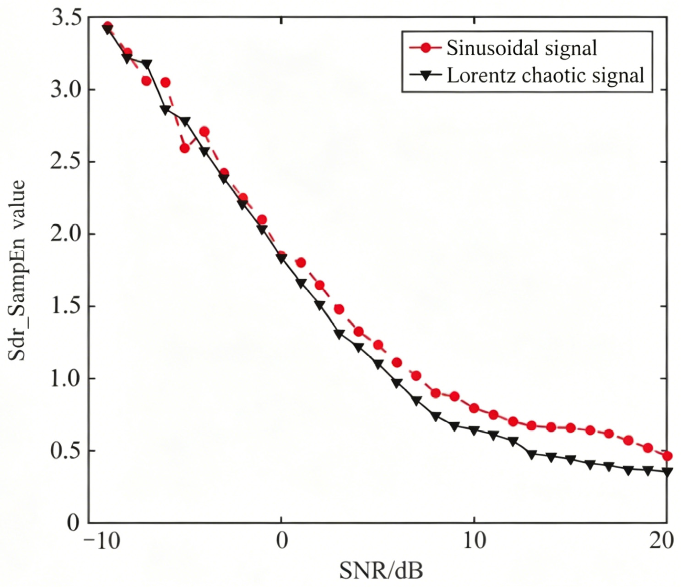
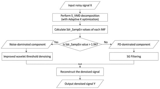
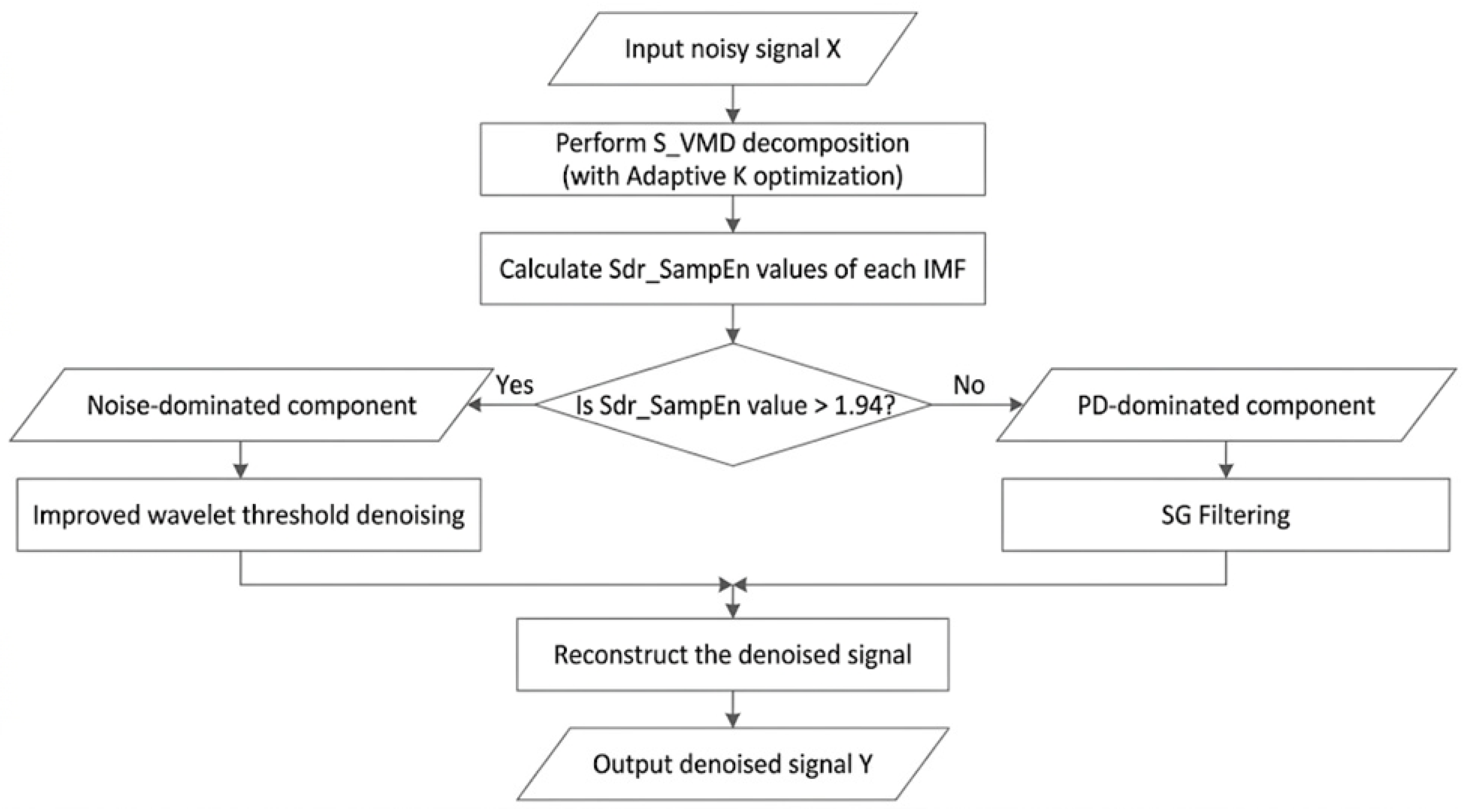
The Sdr_SampEn value at a signal-to-noise ratio of 0 dB is taken as the threshold p and used as an indicator to distinguish between the noise-dominant components and the PD-dominant components. Add Gaussian white noise ranging from −10 dB to 20 dB to the two signals, with a step size of 1 dB. Test 20 times for each step size to obtain the average value of Sdr_SampEn, as shown in Figure 5. From Figure 5, it can be seen that as the signal-to-noise ratio of the two signals continues to increase, the Sdr_SampEn value of the signal also decreases. Therefore, the Sdr_SampEn value has an excellent discriminative effect. The Sdr_SampEn values of the two signals in Figure 5 at 0 dB are both around 1.94, therefore the threshold p is set to 1.94. The process of the algorithm proposed in this article is shown in Figure 6.

Figure 5. Sdr_SampEn value of noisy sinusoidal signal and Lorentz chaotic signal.

Figure 6. Flow chart of the denoising method in this paper.

2.5. PD Signal Generation

The simulated PD and noise signals are generated according to their mathematical model during the Townsend discharge process. Specifically, the PD signal (SPD) can be illustrated via double exponential pulse (DEP), single exponential decay oscillation pulse (SEDOP), and double exponential oscillation pulse (DEOP) [7]. The SEDOP and DEOP in (7) are utilized since they are often recorded by the sensor, which contains the distinct oscillating property caused by the impact of the propagation path and the transfer function of the sensor:

$$S_{PD}\left(t\right)=\mathrm{SEDOP}\left(t\right)+\mathrm{DEOP}\left(t\right)$$

(7)

$$s.t.\{\begin{array}{c}\mathrm{SEDOP}\left(t\right)={\mathsf{\Phi }}_1\cdot {\mathrm{e}}^{-t/{\mathsf{\tau }}_1}\sin \left(2\mathsf{\pi }{f}_{c1}t\right)\\ \mathrm{DEOP}\left(t\right)={\mathsf{\Phi }}_2\cdot \left({\mathrm{e}}^{-t/{\mathsf{\tau }}_2}-{\mathrm{e}}^{-t/{\mathsf{\tau }}_3}\right)\sin \left(2\mathsf{\pi }{f}_{c2}t\right)\end{array}$$

(8)

where the $\Phi$, $\tau$, and $f_c$ denote the oscillation amplitude, time constant, and frequency. The $t$ is record time.

Further, the preset noise signal Snoise consists of discrete spectrum noise (raised by high-order harmonic and communication signals) and periodic narrowband interference (raised by thermal, ground, and random noise), as is illustrated by (8) [18]:

$$S_{\mathrm{noise}}=A_0\left({\mathrm{e}}^{-t/{\mathsf{\tau }}_0}-{\mathrm{e}}^{-t/{\mathsf{\tau }}_s}\right)+\sum _{i=1}^m{A}_i\cdot \sin \left(2\mathsf{\pi }{f}_{ni}t+{\mathsf{\phi }}_i\right)$$

(9)

where $A$ denotes the amplitude of the signal and $m$ denotes the number of periodic components (m = 5), and where $f_{ni}$ represents the oscillation frequency, and $\phi$ denotes the phase angle.

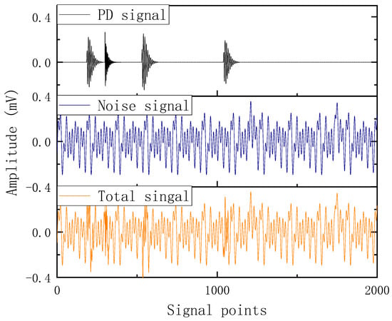
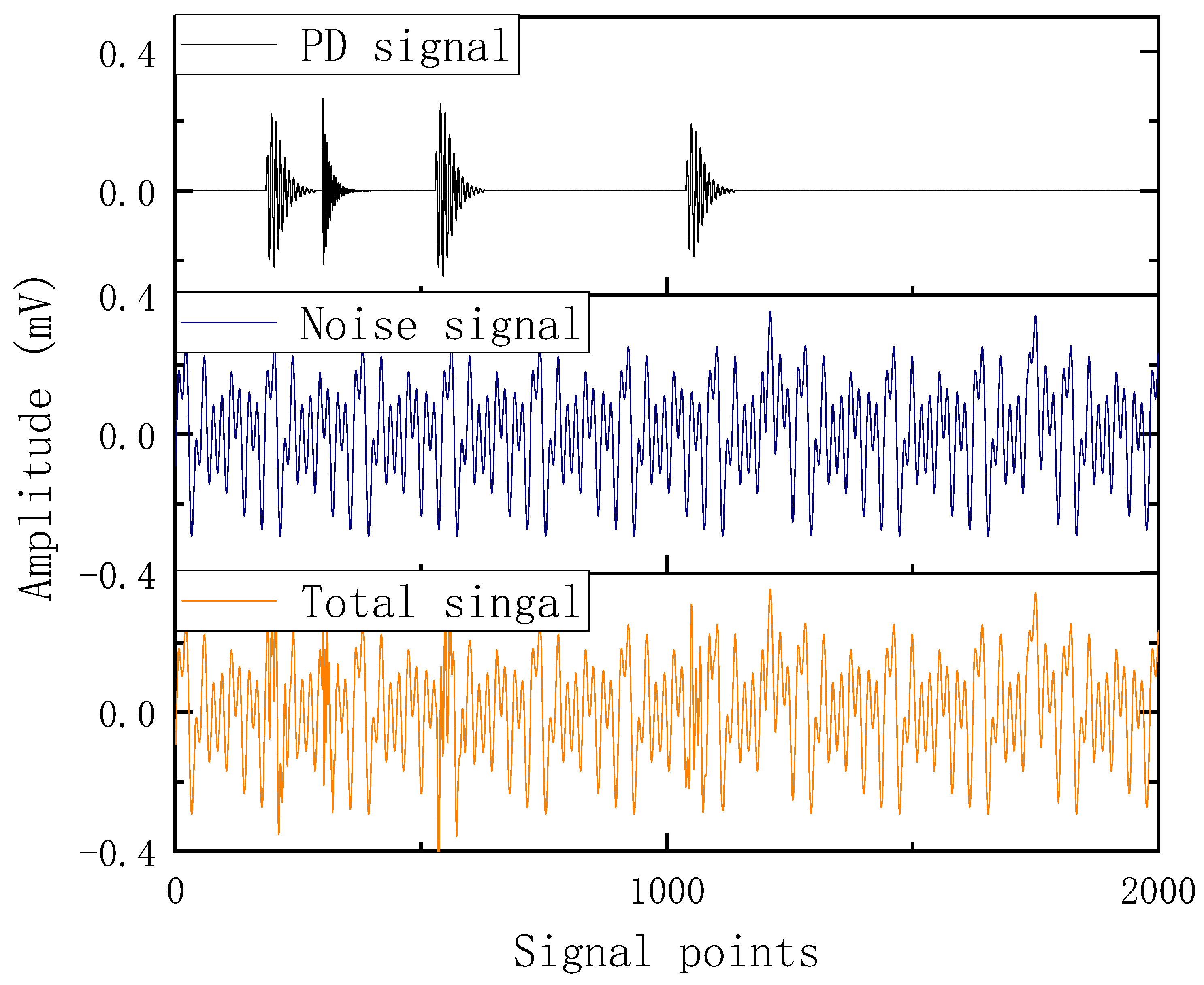
The parameters in (7) and (8) are tabulated in Table 1 for simulating the PD and noise signal. The total signal is the sum of PD and noise, as shown in Figure 7.

Table 1. Parameters for generating pulse and noise signals.

Parameters of PD Signal in (7) and (8)
Items	Φ1	Φ2	τ1	τ2	τ3	fc1	fc2
value	[0.2, 0.4]	[0.9, 1.4]	2.6 × 106	2.17 × 106	3.67 × 106	8 × 106	4 × 106
Items	A0	A1	A2	A3	A4	A5
value	[0.8, 1.2]	0.025	0.05	0.075	0.100	0.125
Items	τ1	fn1	fn2	fn3	fn4	fn5
value	2.6 × 106	0.4 × 106	0.6 × 106	0.8 × 106	1 × 106	2 × 106
Items	τs	φ1	φ2	φ3	φ4	φ5
value	4.4 × 106	π/6	π/4	−π/4	−π/3	0

Figure 7. The simulated PD, noise signal, and the total signal.

2.6. Generation of Actual PD Signals in Lab Condition

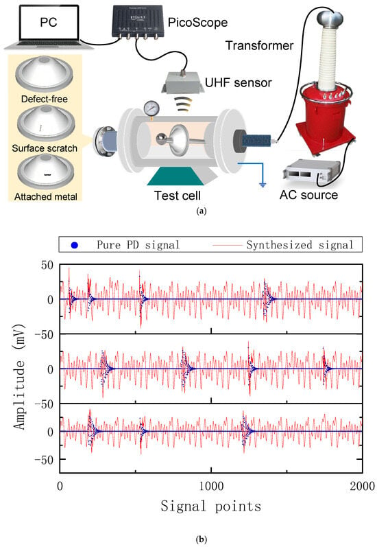
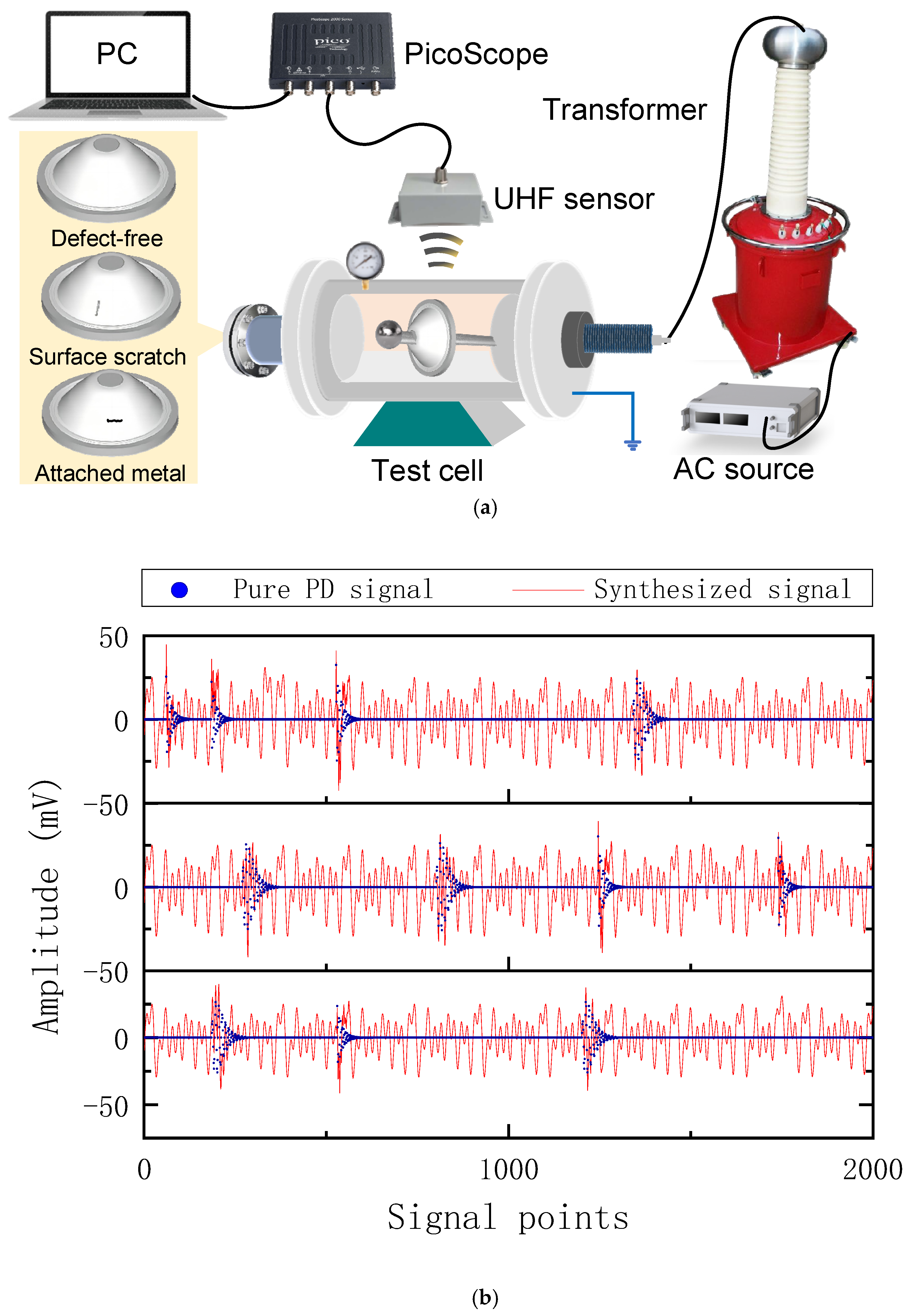
This section aims to collect the actual PD signal to support the accuracy investigation. The epoxy insulation spacers used in previous work are employed to generate the PD signal [19]. The specimen’s profile and the corresponding measurement circuit are plotted in Figure 8a. The test conditions remain at room temperature and maintain 0.3 MPa SF₆. The AC voltage is 6 kV to trigger the distinct PD and then recorded by the UHV sensor (sampling frequency is 1 GS/s), as is shown in Figure 8b. The synthesized signal is the sum of measured pure PD and noise signal simulated by (8).

Figure 8. (a) The experimental platform for generating the actual PD; (b) the actual PD signals and their synthesized signals.

3. Results

3.1. Noise Reduction Evaluation Criteria

In order to evaluate the denoising effect of the algorithm proposed in this paper, the signal-to-noise ratio (SNR), waveform similarity coefficient (NCC), and root mean square error (RMSE) are introduced to assess the denoising effect of the simulated signals [7]. Since it is not possible to obtain a pure PD signal from the measured signals and compute the above three indicators, the noise reduction rate (NRR) is introduced to evaluate the denoising effect of the measured signals, as shown in Equations (10)–(13). Among them, the larger the SNR, the closer the NCC is to one, and the smaller the RMSE, the better the denoising effect; the larger the NRR, the stronger the noise suppression capability.

$$S_{\mathrm{NR}}=10\lg {\displaystyle \frac{{\sum }_{i=1}^N{s}^2\left(i\right)}{{\sum }_{i=1}^N{\left[y\left(i\right)-s\left(i\right)\right]}^2}}$$

(10)

$$N_{\mathrm{CC}}={\displaystyle \frac{{\sum }_{i=1}^{N}s\left(i\right)\cdot y\left(i\right)}{\sqrt{\left({\sum }_{i=1}^N{s}^2\left(i\right)\right)\cdot \left({\sum }_{i=1}^N{y}^2\left(i\right)\right)}}}$$

(11)

$$R_{\mathrm{MSE}}=\sqrt{{\displaystyle \frac{1}{N}}\sum _{i=1}^N{\left[y\left(i\right)-s\left(i\right)\right]}^2}$$

(12)

$$N_{\mathrm{RR}}=10\left(\lg {\mathsf{\sigma }}_1^2-\lg {\mathsf{\sigma }}_2^2\right)$$

(13)

where $s\left(i\right)$ denotes the simulated PD signal; $y\left(i\right)$ represents the denoised signal; $N$ denotes the number of sampling points; ${\sigma }_1$ and ${\sigma }_2$ are the standard deviations of the noisy signal and the denoised signal, respectively.

3.2. Simulation PD Signal Denoising

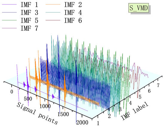
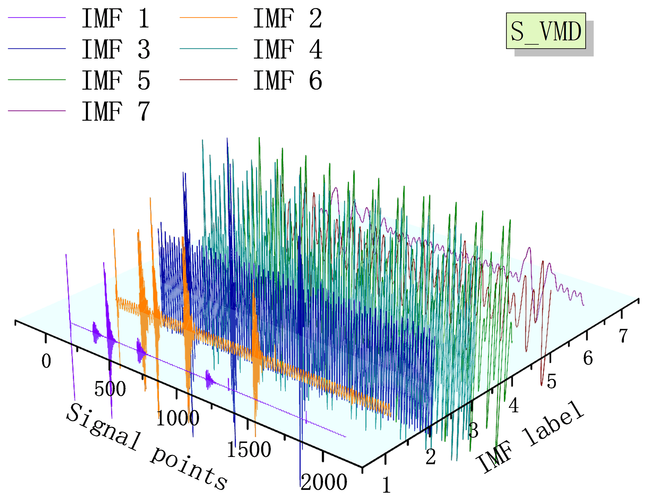
The S_VMD decomposition of the noisy PD signal is shown, with the decomposed IMF1—IMF7 illustrated in Figure 9, and their Sdr_SampEn values displayed in Table 2.

Figure 9. S_VMD decomposition.

Table 2. Sdr_SampEn of every IMF.

IMF	Sdr_SampEn Value
IMF1	0.8563
IMF2	0.7289
IMF3	3.2575
IMF4	2.6748
IMF5	3.4785
IMF6	2.0764
IMF7	1.4396

The significant variance in Sdr_SampEn values among IMFs is directly related to their physical generation mechanisms. Physically, PD is a transient dielectric breakdown characterized by rapid, highly irregular pulses in the time domain, which corresponds to the low entropy values of PD-dominant components (e.g., IMF1 and IMF2). Conversely, noise-dominant components (e.g., IMF5) primarily consist of continuous, steady-state periodic narrowband interferences (such as carrier communications and high-order harmonics) present in the actual electromagnetic environment. This high degree of periodicity physically translates to the significantly higher Sdr_SampEn values.

From Table 2, it can be seen that the Sdr_SampEn values of IMF1, IMF2, and IMF7 are all less than 1.94, indicating that they are PD-dominant components. Among them, the Sdr_SampEn value of IMF7 shows a significant gap compared to IMF1 and IMF2, indicating that IMF1 and IMF2 contain more PD information, and their characteristics as PD-dominant components are also more pronounced than those of IMF7. The Sdr_SampEn values of the other IMFs are all greater than 1.94, indicating they are noise-dominant components. SG filtering is applied to the PD-dominant components, while improved wavelet threshold denoising is used for the noise-dominant components, followed by reconstruction to obtain the denoised PD signal.

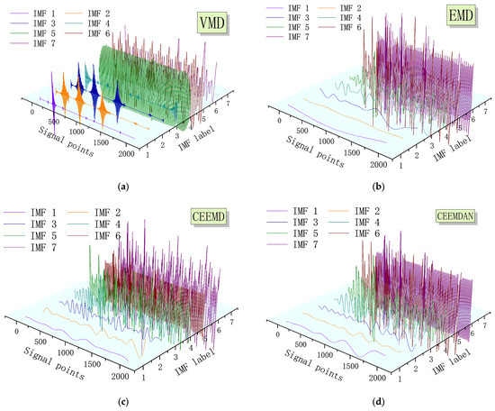
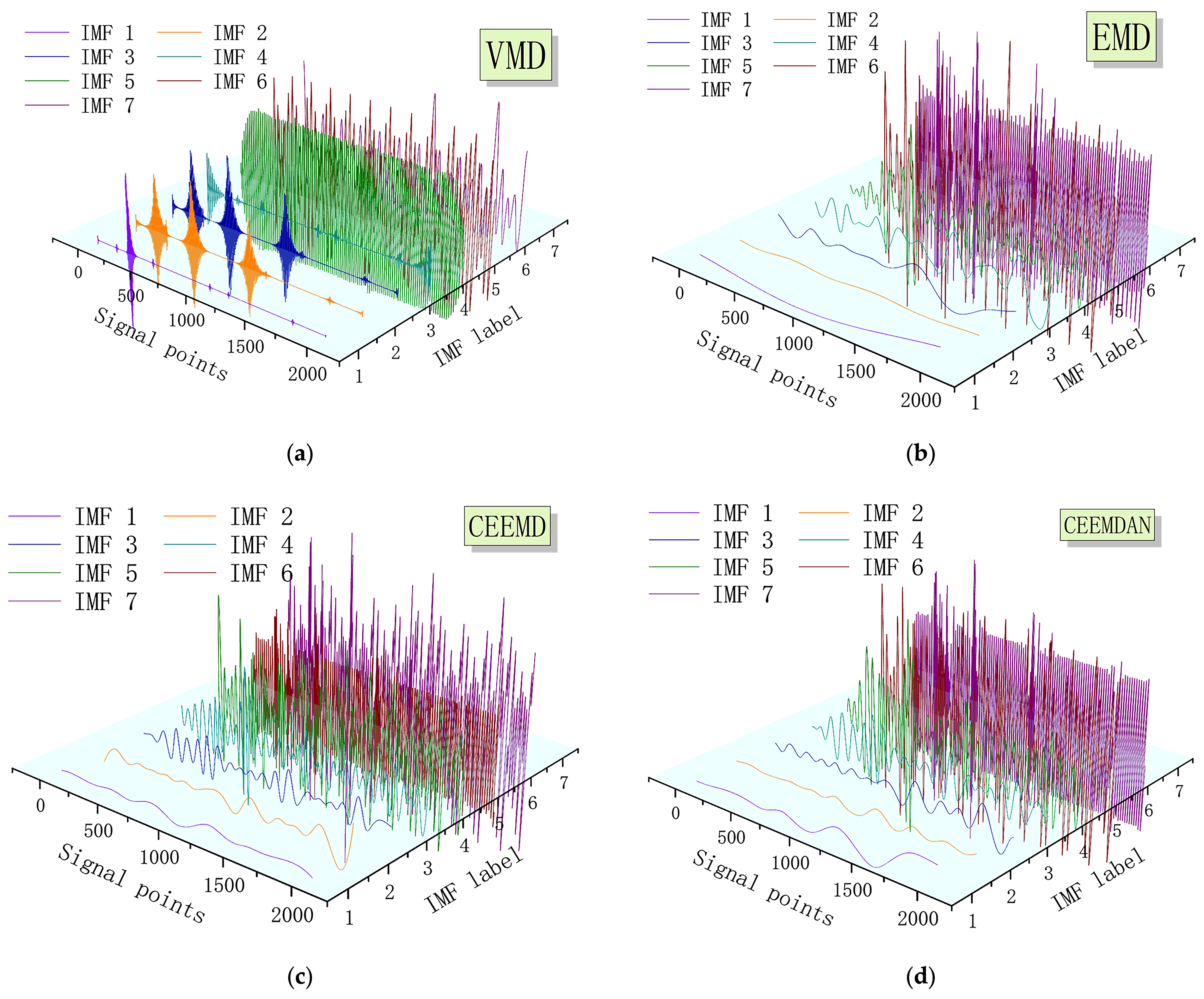
The simulated partial discharge signals obtained in the second section are decomposed using VMD [8], EMD [20], CEEMD [21], and CEEMDAN [22] methods, and the resulting intrinsic mode functions (IMFs) obtained via these four alternative signal decomposition methods are illustrated in Figure 10. Based on the FE of each order IMF, component selection is performed, and for the selected noise-dominant components, both the improved wavelet threshold function proposed in this paper and the traditional wavelet threshold function are used for denoising. At the same time, there are two control groups that do not undergo any signal decomposition treatment, directly applying traditional and improved wavelet threshold denoising to the signals. The denoising results are shown in Table 3. Combining the threshold p used in the Sdr_SampEn algorithm to distinguish between noise-dominant and PD-dominant components for denoising classification, improved wavelet threshold denoising and SG filtering denoising were performed for noise-dominant and partial discharge dominant components, respectively. White noise was added to the pure partial discharge signal to achieve a signal-to-noise ratio of 3 dB. The indicators mentioned in Section 3.1 were used to evaluate different signal decomposition methods, and the results are shown in Table 3. It can be seen that the improved method proposed in this article has better denoising evaluation indicators than the other four algorithms under the same conditions. In addition, due to the complex overall structure of the method proposed in this article, a large number of external functions were called during simulation, resulting in a longer running time of the algorithm, with several simulations lasting up to 5 s. In the subsequent calculation of Sdr_SampEn values, the algorithm parameters can be optimized to improve timeliness.

Figure 10. IMFs obtained via signal decomposition methods. (a) VMD, (b) EMD, (c) CEEMD, (d) CEEMDAN.

Table 3. Denoising results of the analog signal.

Signal Decomposition Method	NCC	RMSE	NRR
VMD	0.8725	0.3512	10.28
EMD	0.8214	0.4185	8.56
CEEMD	0.8903	0.3127	11.14
CEEMDAN	0.9012	0.2986	11.77
S_VMD	0.9628	0.1854	15.32

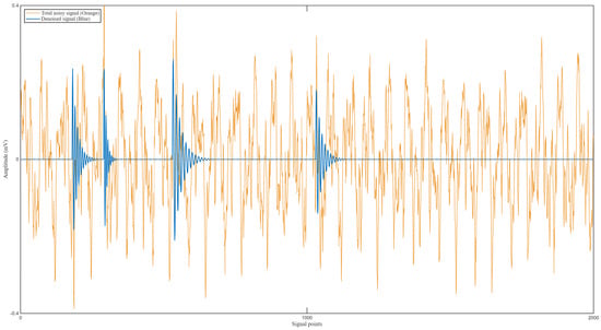
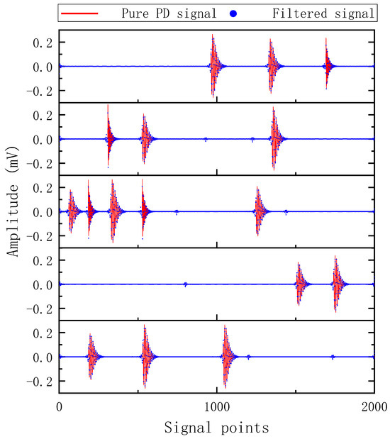
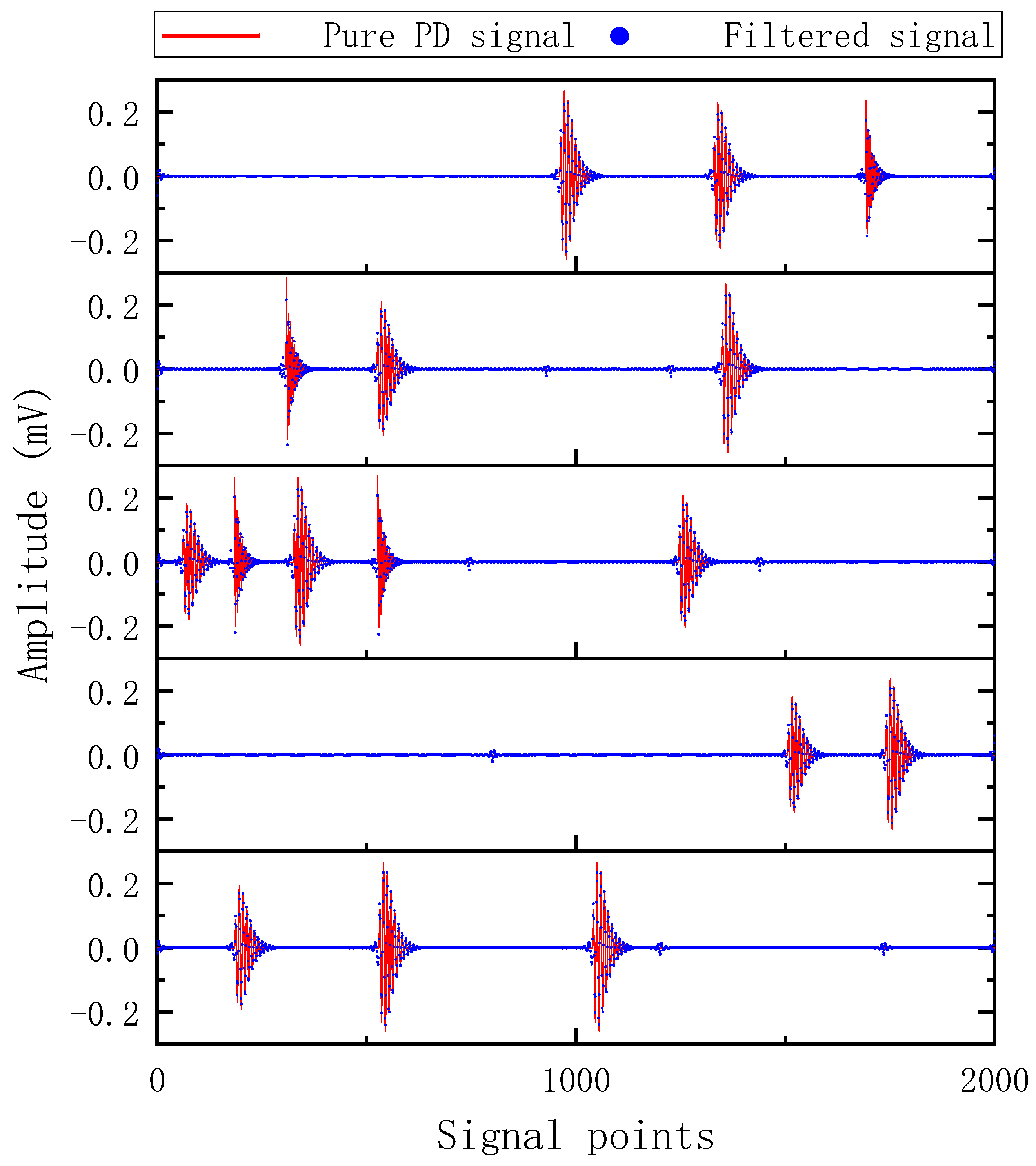
To intuitively evaluate the morphological preservation of the discharge pulses, an overlay plot comparing the original pure PD signal and the denoised waveform is presented in Figure 11. As clearly observed, the denoised signal reconstructed by the pro-posed framework closely tracks the pure PD pulse. The algorithm effectively suppresses the background interference while excellently preserving the steep rising edges and transient oscillatory characteristics. Furthermore, there is no noticeable phase shift or severe amplitude distortion. This visual evidence intuitively validates the capability of the proposed method in maintaining the authentic morphological features of the PD signal during the denoising process.

Figure 11. Overlay plot comparing the pure PD signal and the denoised waveform.

4. Discussion

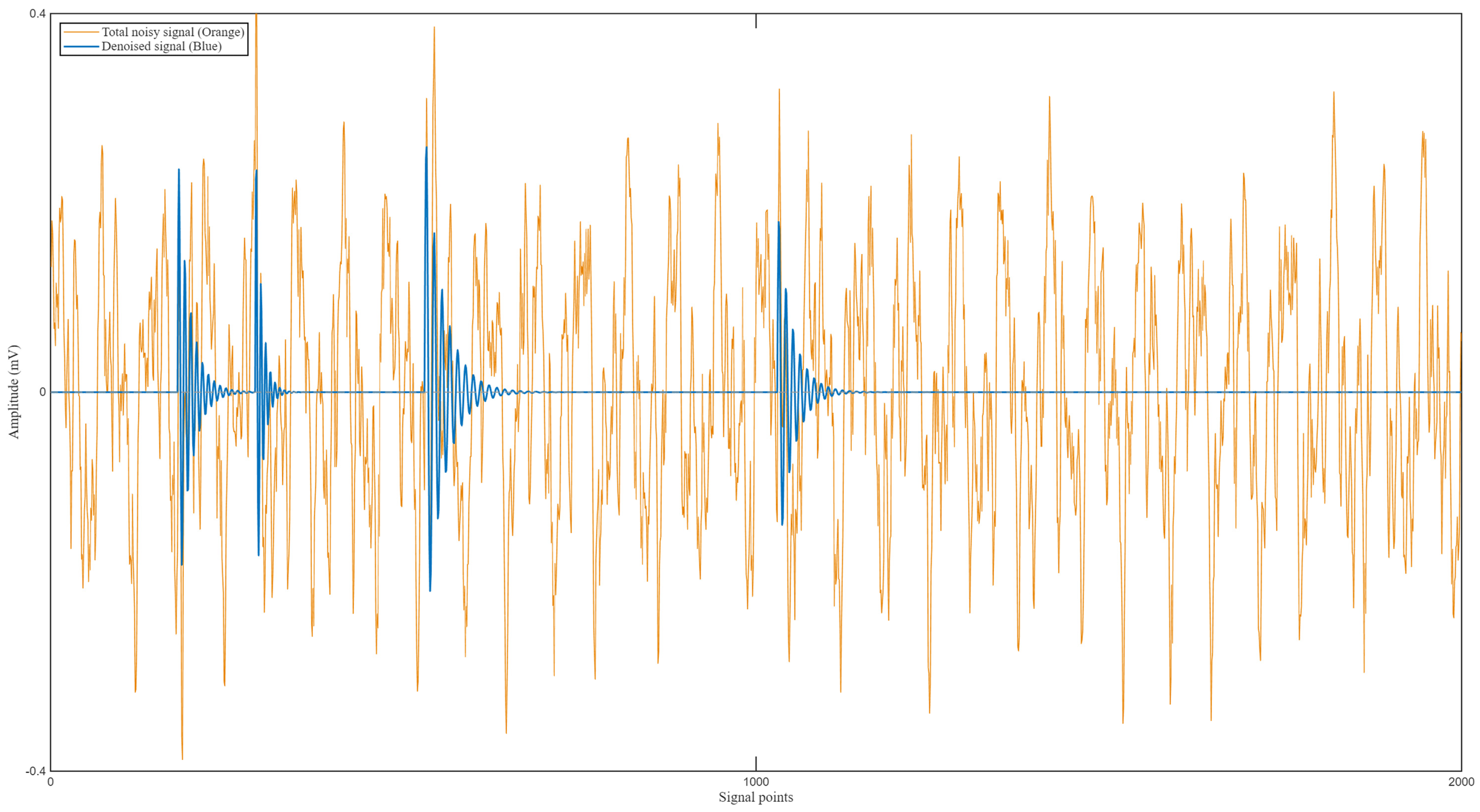
By measuring the partial discharge signal and denoising the measured signal, the effectiveness of the denoising method mentioned in this paper was further verified. On the experimental platform shown in Figure 8a, a voltage was applied to both ends of the wire cavity to measure the actual partial discharge signal, and the above method was used for processing. The denoised signal was compared with the pure local signal as shown in Figure 12. It can be seen from the figure that after denoising with the S_VMD algorithm, the noise of the measured signal can be effectively suppressed. Comparing the NRR of several denoising signals, as shown in Table 4, it can be seen that the denoising method in this paper has the highest NRR and the greatest denoising degree on the measured signal.

Figure 12. Measured signal noise reduction signal diagram.

Table 4. Comparison of measured PD signal denoising effects.

Denoising Method	VMD	EMD	CEEMD	CEEMDAN	S_VMD
NRR	9.39	7.62	11.57	11.39	14.38

By comparing the simulated results in Section 3 with the measured outcomes in this section, it is evident that the theoretical Sdr_SampEn threshold (p = 1.94) calculated from synthesized data exhibits excellent generalization to real-world signals. Furthermore, it is crucial to discuss the impact of time separation and packet overlap. Furthermore, it is crucial to discuss the impact of time separation and packet overlap on the proposed denoising process. Traditional time-domain windowing techniques often struggle or fail when multiple PD pulses are densely superimposed (packet overlap) due to severe phase and amplitude mixing. However, the proposed S_VMD framework exhibits strong robustness against such temporal variations because it operates by adaptively decomposing the signal in the frequency domain rather than the time domain. Background interferences, such as harmonics and carrier signals, inherently manifest as steady-state, narrowband periodic waves. In contrast, PD pulses—whether occurring as isolated events with large time separation or densely overlapping bursts—maintain their broadband, high-frequency transient nature. Consequently, even under severe packet overlap, S_VMD can effectively isolate periodic noise into specific IMFs based on their distinct frequency characteristics.

Additionally, packet overlap directly affects the proposed spatial-temporal evaluation indicator, Sdr_SampEn. When PD pulses overlap, the temporal irregularity, abruptness, and structural complexity of the signal actually increase. This increased chaos ensures that the overlapping PD components maintain extremely low Sdr_SampEn values, remaining strictly below the calibrated classification threshold (p = 1.94). As a result, densely overlapping PD pulses are accurately recognized as PD-dominant components rather than noise. They are then faithfully preserved and smoothed during the subsequent Savitzky–Golay filtering stage. This demonstrates the inherent advantage of the proposed S_VMD and Sdr_SampEn combined framework in handling complex, high-density discharge scenarios in practical GIS engineering.

5. Conclusions

This paper proposes a hybrid denoising framework for GIS partial discharge signals that combines Spearman-optimized VMD, spatially related recursive sample entropy, an improved wavelet threshold function and Savitzky–Golay filtering. The main conclusions are as follows.

• Using the Spearman correlation coefficient between the original signal and its VMD reconstruction as the stopping criterion, the optimal mode number is adaptively determined. For the PD signals considered in this work, K = 7 is sufficient to reach a correlation coefficient of 0.99, avoiding both under- and over-decomposition;
• The proposed Sdr_SampEn indicator quantifies signal irregularity along both the Chebyshev-distance and spatial directions of a recurrence plot, and can reliably distinguish PD-dominant from noise-dominant IMFs. Calibrated at 0 dB, a threshold of p = 1.94 is shown to be effective for the tested signals;
• The improved wavelet threshold function is continuous at ±λ and asymptotically un-biased, overcoming the oscillation artifacts of the hard threshold and the fixed bias of the soft threshold. Combined with SG filtering for the PD-dominant components, it yields faithful reconstruction of PD pulse morphology;
• On simulated PD signals at 3 dB input SNR, the proposed S_VMD-based method achieves NCC = 0.9628, RMSE = 0.1854 and NRR = 15.32, clearly outperforming VMD, EMD, CEEMD and CEEMDAN. On measured signals from epoxy spacers with typical defects, it yields NRR = 14.38, again the best among the compared methods.;

The main limitation of the current implementation is computational cost: a single denoising run can take up to 5 s because of the iterative parameter search in Sdr_SampEn. Future work will focus on (i) accelerating the algorithm through parameter pre-tabulation and GPU parallelization, (ii) extending the validation to a broader range of PD defect types (corona, floating electrode and free particle) and on-site field data, and (iii) coupling the proposed denoising front-end with a deep learning-based classifier to build a complete end-to-end GIS PD fault-diagnosis pipeline.

References

- Li, C.; Hu, J.; Lin, C.; Zhang, B.; Zhang, G.; He, J. Surface Charge Migration and Dc Surface Flashover of Surface-Modified Epoxy-Based Insulators. J. Phys. Appl. Phys. 2017, 50, 065301. [Google Scholar] [CrossRef] [Scilit]
- Stone, G.C.; Sedding, H.G.; Chan, C. Experience with Online Partial-Discharge Measurement in High-Voltage Inverter-Fed Motors. IEEE Trans. Ind. Appl. 2018, 54, 866–872. [Google Scholar] [CrossRef] [Scilit]
- Tenbohlen, S.; Denissov, D.; Hoek, S.; Markalous, S.M. Partial Discharge Measurement in the Ultra High Frequency (UHF) Range. IEEE Trans. Dielectr. Electr. Insul. 2008, 15, 1544–1552. [Google Scholar] [CrossRef] [Scilit]
- Zhao, R.-M.; Cui, H. Improved Threshold Denoising Method Based on Wavelet Transform. In Proceedings of the 2015 7th International Conference on Modelling, Identification and Control (ICMIC), Sousse, Tunisia, 18–20 December 2015; pp. 1–4. [Google Scholar]
- Wu, Z.; Huang, N.E. A Study of the Characteristics of White Noise Using the Empirical Mode Decomposition Method. Proc. R. Soc. Lond. Ser. Math. Phys. Eng. Sci. 2004, 460, 1597–1611. [Google Scholar] [CrossRef] [Scilit]
- Chan, J.C.; Ma, H.; Saha, T.K. Hybrid Method on Signal De-noising and Representation for Online Partial Discharge Monitoring of Power Transformers at Substations. IET Sci. Meas. Technol. 2015, 9, 890–899. [Google Scholar] [CrossRef] [Scilit]
- Lei, Z.; Wang, F.; Li, C. A Denoising Method of Partial Discharge Signal Based on Improved SVD-VMD. IEEE Trans. Dielectr. Electr. Insul. 2023, 30, 2107–2116. [Google Scholar] [CrossRef] [Scilit]
- Fang, W.; Chen, G.; Li, W.; Xu, M.; Xie, W.; Chen, C.; Wang, W.; Zhu, Y. A PRPD-Based UHF Filtering and Noise Reduction Algorithm for GIS Partial Discharge. Sensors 2023, 23, 6763. [Google Scholar] [CrossRef] [Scilit] [PubMed]
- Vincent, P.; Larochelle, H.; Lajoie, I.; Bengio, Y.; Manzagol, P.-A. Stacked Denoising Autoencoders: Learning Useful Representations in a Deep Network with a Local Denoising Criterion. J. Mach. Learn. Res. 2010, 11, 3371–3408. [Google Scholar]
- Gondara, L. Medical Image Denoising Using Convolutional Denoising Autoencoders. In Proceedings of the 2016 IEEE 16th International Conference on Data Mining Workshops (ICDMW), Barcelona, Spain, 12–15 December 2016; pp. 241–246. [Google Scholar]
- Jiang, C.; Chen, Y.; Chen, S.; Bo, Y.; Li, W.; Tian, W.; Guo, J. A Mixed Deep Recurrent Neural Network for MEMS Gyroscope Noise Suppressing. Electronics 2019, 8, 181. [Google Scholar] [CrossRef] [Scilit]
- Ali Abd AlHameed, K. Spearman’s Correlation Coefficient in Statistical Analysis. Int. J. Nonlinear Anal. Appl. 2022, 13, 3249–3255. [Google Scholar] [CrossRef]
- Altieri, L.; Cocchi, D.; Roli, G. Advances in Spatial Entropy Measures. Stoch. Environ. Res. Risk Assess. 2019, 33, 1223–1240. [Google Scholar] [CrossRef] [Scilit]
- Zhang, Y.; Ding, W.; Pan, Z.; Qin, J. Improved Wavelet Threshold for Image De-Noising. Front. Neurosci. 2019, 13, 39. [Google Scholar] [CrossRef] [Scilit] [PubMed]
- Krishnan, S.R.; Seelamantula, C.S. On the Selection of Optimum Savitzky-Golay Filters. IEEE Trans. Signal Process. 2013, 61, 380–391. [Google Scholar] [CrossRef] [Scilit]
- Duan, Y.; Song, C. Relevant Modes Selection Method Based on Spearman Correlation Coefficient for Laser Signal Denoising Using Empirical Mode Decomposition. Opt. Rev. 2016, 23, 936–949. [Google Scholar] [CrossRef] [Scilit]
- Jia, K.; Yang, Z.; Zheng, L.; Zhu, Z.; Bi, T. Spearman Correlation-Based Pilot Protection for Transmission Line Connected to PMSGs and DFIGs. IEEE Trans. Ind. Inform. 2021, 17, 4532–4544. [Google Scholar] [CrossRef] [Scilit]
- Yan, Y.; Trinchero, R.; Stievano, I.S.; Li, H.; Xie, Y.-Z. An Automatic Tool for Partial Discharge De-Noising via Short-Time Fourier Transform and Matrix Factorization. IEEE Trans. Instrum. Meas. 2022, 71, 1–12. [Google Scholar] [CrossRef] [Scilit]
- Fan, X.; Luo, H.; Liang, F.; Hu, J.; Liu, W.; Li, C.; He, J. Photon Count Technique as a Potential Tool for Insulation Micro-Defect Detection: Principles and Primary Results. iEnergy 2023, 2, 258–263. [Google Scholar] [CrossRef] [Scilit]
- Shams, M.A.; Anis, H.I.; El-Shahat, M. Denoising of Heavily Contaminated Partial Discharge Signals in High-Voltage Cables Using Maximal Overlap Discrete Wavelet Transform. Energies 2021, 14, 6540. [Google Scholar] [CrossRef] [Scilit]
- Sun, K.; Wu, T.; Li, X.; Zhang, J. Robust Estimation of Arrival Time of Complex Noisy Partial Discharge Pulse in Power Cables Based on Adaptive Variational Mode Decomposition. Appl. Sci. 2020, 10, 1641. [Google Scholar] [CrossRef] [Scilit]
- Sun, K.; Zhang, J.; Shi, W.; Guo, J. Extraction of Partial Discharge Pulses from the Complex Noisy Signals of Power Cables Based on CEEMDAN and Wavelet Packet. Energies 2019, 12, 3242. [Google Scholar] [CrossRef] [Scilit]
Disclaimer/Publisher’s Note: The statements, opinions and data contained in all publications are solely those of the individual author(s) and contributor(s) and not of MDPI and/or the editor(s). MDPI and/or the editor(s) disclaim responsibility for any injury to people or property resulting from any ideas, methods, instructions or products referred to in the content. |
© 2026 by the authors. Licensee MDPI, Basel, Switzerland. This article is an open access article distributed under the terms and conditions of the Creative Commons Attribution (CC BY) license.