A Dynamic Harmonic Coupling Matrix Modeling Approach for Power Quality Analysis in Electric Vehicle Charging Stations with Bidirectional Capability

Abstract

The proliferation of large-scale electric vehicle charging stations has made power quality issues increasingly prominent. While conventional unidirectional charging stations already present complex harmonic interactions, the development of vehicle-to-grid technology has introduced more complex harmonic coupling in bidirectional charging stations. To improve the accuracy of harmonic power flow analysis, this paper proposes a hybrid mechanism–data-driven dynamic harmonic coupling matrix model (DHCMM) for power quality assessment in bidirectional charging stations. A DHCMM-based harmonic power flow calculation process is further developed to evaluate the harmonic impact on power distribution networks following station integration. The proposed method is validated using field measurement data from an actual bidirectional charging station with tests covering typical charging, discharging, and dynamic transition scenarios. Results show that the DHCMM provides accurate harmonic modeling with both the total harmonic current distortion estimation error and the voltage fluctuation estimation error within 5%. The validated model is applied to an IEEE 33-bus distribution system. A comparison of the results reveals that the power quality impact of such stations extends beyond the point of connection to neighboring nodes, while the proposed DHCMM outperforms mechanism-based models including the static harmonic coupling matrix model and the Norton harmonic equivalent model as well as data-driven models such as the backpropagation neural network and least squares support vector machines.

1. Introduction

The rapid advancement of electric vehicles and charging technologies has significantly accelerated the expansion of charging infrastructure. Bidirectional charging stations, enabling vehicle-to-grid (V2G) interaction, are becoming widespread [1,2]. However, the large-scale grid integration of multi-type chargers in such stations, along with frequent switching between charging and discharging modes, can trigger power quality issues such as voltage fluctuations and harmonic distortions [3,4,5,6,7]. Therefore, evaluating harmonic conditions in distribution networks is essential to clarify grid integration impacts and guide mitigation strategies.

Traditional harmonic modeling is primarily divided into mechanism-based [8,9,10,11,12,13,14] and data-driven methods [15,16,17,18,19,20]. Early mechanism-based methods used constant current source models that neglect frequency coupling and rely on static data, limiting accuracy under dynamic conditions. The harmonic state-space method has been introduced to address coupling in periodic time-varying systems [21] and improves stability evaluation for multi-converter systems [22]. But this method relies heavily on the physical parameters and charger topologies, making it impractical for stations where internal parameters are often unavailable.

To characterize the multi-frequency coupling between voltage and current at the ports of nonlinear devices, admittance matrix modeling methods based on frequency coupling characteristics have been widely adopted. A frequency-coupled admittance model for grid-connected converters analyzed the impact of control loops on multi-frequency harmonic interactions [23], and it was later extended to electric vehicle charging stations [24]. However, such mechanism-based methods rely on small-signal linearization and accurate topologies/parameters. Consequently, their accuracy and practicality are inadequate for harmonic sources in various charging stations, which feature strong uncertainties and time-varying behavior.

With the advancement of data sensing technologies, data-driven modeling has emerged as a systematic and versatile approach. The Norton harmonic equivalent model (NHEM) has been adopted to simplify harmonic representation of nonlinear loads, but this model ignores the coupling between harmonic voltages and currents, leading to increased impedance errors under varying voltage conditions [25]. Improved partial least squares methods have been proposed for robust harmonic emission estimation by suppressing measurement noise and multicollinearity, yet they remain constrained by linear regression frameworks and struggle with strong nonlinearities [26]. Recursive least squares methods have enabled the real-time detection and tracking of dynamic harmonic features [27].

More recently, data-driven methods such as Least Squares Support Vector Machines (LS-SVMs) and radial basis function neural networks have been emerged [28]. However, while LS-SVMs achieve high precision with small samples and nonlinear mapping, they suffer from high kernel computation overhead and generalization challenges when handling massive data. Nevertheless, existing data-driven methods generally overlook the dynamic evolution of harmonic frequency coupling caused by operational mode switching in charging stations, making them insufficiently accurate and adaptable for highly time-varying harmonic sources.

Currently, mechanism-based and data-driven methods are often treated as separate paradigms, yet they are inherently complementary. Thus, an integrated approach that combines the merits of both has become critical for improving harmonic evaluation accuracy in distribution networks. This paper proposes a dynamic harmonic coupling matrix model (DHCMM) that bridges the gap between mechanism-based and data-driven approaches, enabling accurate harmonic modeling for charging stations while effectively capturing the additional complexity introduced by bidirectional operation.

Furthermore, the proposed DHCMM introduces a voltage similarity index on the basis of the harmonic coupling matrix model (HCMM) to realize the recursive update of matrix coefficients. Compared with mechanism-based models including the NHEM [29] and the Static Harmonic Coupling Matrix Model (SHCMM) [30], as well as data-driven models such as Backpropagation Neural Network (BPNN) [31] and LS-SVM [32], this DHCMM effectively avoids the high dependence on the massive data of such models, while overcoming the shortcomings of fixed and non-adjustable post-training parameters and poor adaptability to complex harmonic modeling under dynamic operating conditions. The characteristic comparisons of different methods are presented in Table 1.

Table 1. Comparisons between DHCMM and existing harmonic modeling methods.

Method	Model Type	Dynamic/Static	Model Structure	Applicable Scenarios
DHCMM (proposed)	Mechanism-data-hybrid-driven Model	Dynamic	Harmonic Coupling Matrix Structure with Dynamic Feedback Unit	Complex Dynamic Harmonic Variations
NHEM [32]	Mechanism-based Model	Static	Traditional Harmonic Decomposition Structure	Stable Harmonic Characteristics and Small Load Fluctuations
SHCMM [33]	Mechanism-based Model	Static	Simplified Static Harmonic Coupling Structure	Stable Harmonic Coupling with Minor Operating Condition Variations
BPNN [34]	Data-driven Model	Static (Fixed After Training)	Multi-Layer Feedforward Neural Network Structure	Sufficient Data and Complex Mechanisms Difficult to Model
LS-SVM [35]	Data-driven Model	Static (Fixed After Training)	Improved Structure Based on Support Vector Machine	Small Samples, Nonlinear Harmonics, and Minor Operating Variations

The main contributions of this paper are as follows:

(1)

A DHCMM tailored for electric vehicle charging stations considering bidirectional V2G capability is proposed. This model constructs a harmonic coupling matrix from measured data and introduces a voltage similarity criterion to dynamically update parameters, thereby dynamically tracking the coupling relationship between harmonic voltages and currents of different frequencies under varying operating conditions.

(2)

A DHCMM-based harmonic power flow calculation method is developed. By incorporating topological characteristics of the distribution network, a forward–backward sweep method based on loop currents is adopted. The DHCMM, constructed from measured data under different scenarios, is injected into the distribution network as a harmonic source to simulate and analyze the voltage variation characteristics at each node.

(3)

Experimental and simulation validation using field data from a bidirectional charging station in China under six scenarios. The DHCMM achieves higher accuracy than the NHEM, SHCMM, BPNN, and LS-SVM with the total harmonic current distortion estimation error and the voltage fluctuation estimation error both within 5%.

The remainder of this paper is organized as follows. Section 2 analyzes the harmonic characteristics of bidirectional charging stations and constructs the DHCMM. Section 3 derives the DHCMM-based harmonic power flow calculation procedure. Section 4 constructs the DHCMM for six scenarios with real-world measured data and simulates the impact of its grid integration on the distribution network. Section 5 concludes the paper.

2. Data-Driven Dynamic Harmonic Coupling Matrix Modeling

2.1. HCMM Based on Measured Data

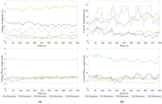
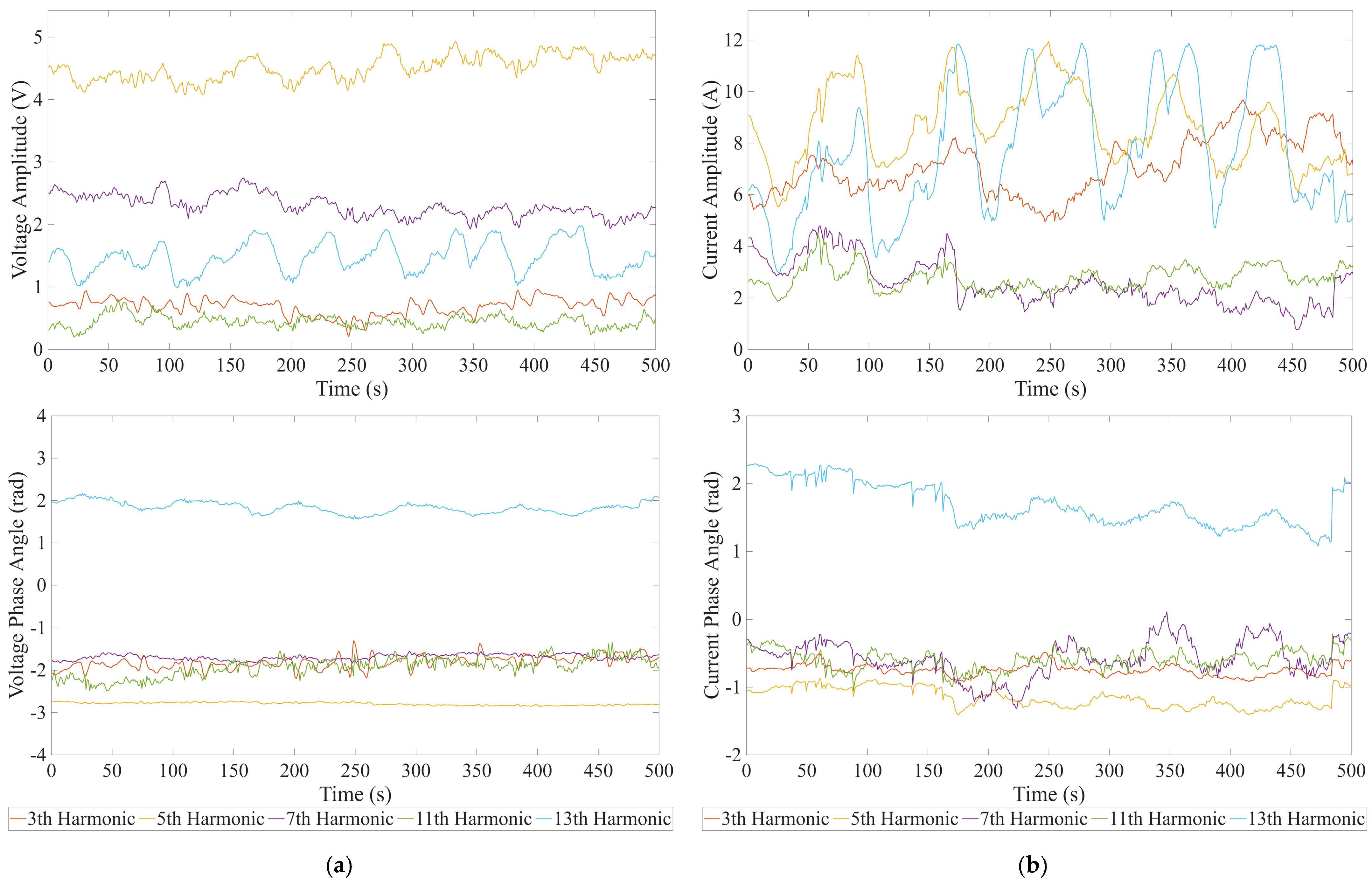
Treating charging stations as a specific type of load, Figure 1 illustrates the measured A-phase voltage and current characteristics at the low-voltage side of a bidirectional charging station node. The measured data show that the fundamental voltage fluctuates between 228 V and 233 V, which is accompanied by substantial dynamic variations in both the magnitudes and phase angles of harmonic voltages. Furthermore, variations in harmonic current magnitudes and phase angles correlate with the fundamental current magnitude, whereas fluctuations in harmonic current phase angles remain relatively mild.

Figure 1. Variation trends of measured voltage and current at a bidirectional charging station. (a) Measured voltage; (b) measured current.

Building upon these characteristics, the harmonic coupling model can be established. The maximum harmonic order H is defined as 13, and the retained harmonics cover the 3rd, 5th, 7th, 9th, 11th and 13th orders. Its mathematical expression is shown as follows:

$$\left[\begin{array}{c}{\dot{I}}_1\\ {\dot{I}}_2\\ ⋮\\ {\dot{I}}_h\\ ⋮\\ {\dot{I}}_H\end{array}\right]=\left[\begin{array}{ccccc}{Y}_{11}& \cdots & Y_{1k}& \cdots & Y_{1H}\\ Y_{31}& \cdots & Y_{3_k}& \cdots & Y_{3H}\\ ⋮& \ddots & ⋮& \ddots & ⋮\\ Y_{h1}& \cdots & Y_{hk}& \cdots & Y_{hH}\\ ⋮& \ddots & ⋮& \ddots & ⋮\\ Y_{H1}& \cdots & Y_{Hk}& \cdots & Y_{HH}\end{array}\right]\left[\begin{array}{c}{\dot{U}}_1\\ {\dot{U}}_3\\ ⋮\\ {\dot{U}}_k\\ ⋮\\ {\dot{U}}_H\end{array}\right]$$

(1)

where ${\dot{I}}_h$ denotes the phasor form of the h-th harmonic current; ${\dot{U}}_k$ represents the phasor form of the k-th harmonic voltage; $Y_{hk}$ characterizes the coupling relationship between the h-th harmonic current and the k-th harmonic voltage; and H is the maximum harmonic order considered in the model; and the harmonic coupling matrix in this equation is an $H\times H$ square matrix containing $H^2$ unknown parameters.

To determine the model parameters, a complex-domain least squares method is applied to the measured A-phase voltage and current data from the charging station node to quantify the harmonic coupling across different frequencies with the source-load harmonic model formulated as

$$\left[\begin{array}{ccc}{\dot{I}}_1(1)& \cdots & {\dot{I}}_1(n)\\ {\dot{I}}_3(1)& \cdots & {\dot{I}}_3(n)\\ ⋮& \ddots & ⋮\\ {\dot{I}}_h(1)& \cdots & {\dot{I}}_h(n)\\ ⋮& \ddots & ⋮\\ {\dot{I}}_H(1)& \ddots & {\dot{I}}_H(n)\end{array}\right]=\left[\begin{array}{ccccc}{Y}_{11}& \cdots & Y_{1k}& \cdots & Y_{1H}\\ Y_{31}& \cdots & Y_{3_k}& \cdots & Y_{3H}\\ ⋮& \ddots & ⋮& \ddots & ⋮\\ Y_{h1}& \cdots & Y_{hk}& \cdots & Y_{hH}\\ ⋮& \ddots & ⋮& \ddots & ⋮\\ Y_{H1}& \cdots & Y_{Hk}& \cdots & Y_{HH}\end{array}\right]\left[\begin{array}{ccc}{\dot{U}}_1(1)& \cdots & {\dot{U}}_1(n)\\ {\dot{U}}_3(1)& \cdots & {\dot{U}}_3(n)\\ ⋮& \ddots & ⋮\\ {\dot{U}}_k(1)& \cdots & {\dot{U}}_k(n)\\ ⋮& \ddots & ⋮\\ {\dot{U}}_H(1)& \cdots & {\dot{U}}_H(n)\end{array}\right]$$

(2)

where ${\dot{I}}_h(n)$ denotes the h-th harmonic current data obtained from the n-th measurement set; and ${\dot{U}}_k(n)$ represents the k-th harmonic voltage data obtained from the n-th measurement set.

The matrix expression in Equation (2) can be further simplified as

$$\mathit{I}=\mathit{Y}\mathit{U}$$

(3)

where I denotes the matrix consisting of the h-th harmonic current data obtained from n sets of measurements; U represents the matrix consisting of the k-th harmonic voltage data obtained from n sets of measurements; and Y denotes the harmonic coupling admittance matrix constructed by fitting the measured data.

The elements on the main diagonal and their adjacent elements in the same row of the harmonic coupling model have relatively large magnitudes, and the harmonic current presents coupling relationships with both the same-order and adjacent-order harmonic voltages [36]. Based on the above analysis, to reduce model complexity while preserving core coupling characteristics, the dominant components with high coupling degrees, including the first-column elements, the main diagonal elements, and their adjacent elements in the same row, are selected to construct the source-load harmonic coupling model. By neglecting elements with lower coupling degrees, the HCMM is reduced to a simplified form that retains only the dominant harmonic coupling components:

$$\left[\begin{array}{ccc}{\dot{I}}_1(1)& \cdots & {\dot{I}}_1(n)\\ {\dot{I}}_3(1)& \cdots & {\dot{I}}_3(n)\\ ⋮& \ddots & ⋮\\ {\dot{I}}_h(1)& \cdots & {\dot{I}}_h(n)\\ ⋮& \ddots & ⋮\\ {\dot{I}}_H(1)& \ddots & {\dot{I}}_H(n)\end{array}\right]=\left[\begin{array}{cccccc}{Y}_{11}& Y_{13}& 0& \cdots & \cdots & 0\\ Y_{31}& Y_{33}& Y_{35}& 0& \ddots & 0\\ ⋮& 0& ⋮& \ddots & ⋮& ⋮\\ Y_{h1}& \cdots & Y_{h(h-2)}& Y_{hh}& Y_{h(h+2)}& ⋮\\ ⋮& \ddots & ⋮& \ddots & ⋮& 0\\ Y_{H1}& 0& \cdots & 0& Y_{H(H-2)}& Y_{HH}\end{array}\right]\left[\begin{array}{ccc}{\dot{U}}_1(1)& \cdots & {\dot{U}}_1(n)\\ {\dot{U}}_3(1)& \cdots & {\dot{U}}_3(n)\\ ⋮& \ddots & ⋮\\ {\dot{U}}_k(1)& \cdots & {\dot{U}}_k(n)\\ ⋮& \ddots & ⋮\\ {\dot{U}}_H(1)& \cdots & {\dot{U}}_H(n)\end{array}\right]$$

(4)

Analysis and verification demonstrate that the first-column elements, the main diagonal elements, and their row-wise adjacent elements in the HCMM are dominant components with high coupling degrees. Simplifying the HCMM based on these dominant elements reduces model complexity while maintaining high fitting accuracy. Consequently, the harmonic characteristic relationship of the charging and discharging station load can be expressed as:

$${\dot{I}}_h={\dot{I}}_{sh}+Y_{h(h-2)}{\dot{U}}_{h-2}+Y_{hh}{\dot{U}}_h+Y_{h(h+2)}{\dot{U}}_{h+2}$$

(5)

where ${\dot{I}}_h$ and ${\dot{U}}_h$ denote the h-th harmonic current and voltage phasors, respectively; ${\dot{I}}_{sh}$ represents the contribution of the first-column elements in the model to the harmonic current, physically manifesting as a current source; and $Y_{hh}$ and $Y_{h(h\pm 2)}$ represent the main diagonal elements and their row-wise adjacent elements of the HCMM, respectively.

To solve for the elements in the HCMM, for the h-th $(3<h<\mathrm{H})$ harmonic, where H denotes the maximum harmonic order considered, the following solution equation is constructed based on the measured voltage and current data:

$$\left[\begin{array}{c}{\dot{I}}_h(1)\\ {\dot{I}}_h(2)\\ ⋮\\ {\dot{I}}_h(i)\\ ⋮\\ {\dot{I}}_h(n)\end{array}\right]=\left[\begin{array}{cccc}1& {\dot{U}}_{h-2}(1)& {\dot{U}}_h(1)& {\dot{U}}_{h+2}(1)\\ 1& {\dot{U}}_{h-2}(2)& {\dot{U}}_h(2)& {\dot{U}}_{h+2}\left(2\right)\\ ⋮& ⋮& ⋮& ⋮\\ 1& {\dot{U}}_{h-2}(i)& {\dot{U}}_h(i)& {\dot{U}}_{h+2}(i)\\ ⋮& ⋮& ⋮& ⋮\\ 1& {\dot{U}}_{h-2}(n)& {\dot{U}}_h\left(n\right)& {\dot{U}}_{h+2}\left(n\right)\end{array}\right]\left[\begin{array}{c}{\dot{I}}_{sh}\\ Y_{h(h-2)}\\ Y_{hh}\\ Y_{h(h+2)}\end{array}\right]$$

(6)

where ${\dot{U}}_h(i)$ and ${\dot{I}}_h(i)$ denote the h-th harmonic voltage and current data from the i-th measurement set, respectively; while n represents the total number of voltage and current data sets measured within the same time interval. For the 3rd and H-th harmonics, elements that do not exist in the above equation can be set to zero.

The first row of the coefficient matrix corresponds to the harmonic current source term ${\dot{I}}_{sh}$, the third row corresponds to the self-admittance $Y_{hh}$, and the second and fourth rows correspond to the mutual admittances $Y_{h(h-2)}$ and $Y_{h(h+2)}$, respectively. These elements are the dominant components retained from the coupling matrix in Equation (1). Equation (6) can be further rewritten as

$${\mathit{I}}_h(n)={\mathit{J}}_h(n){\mathit{M}}_h(n)$$

(7)

where ${\mathit{I}}_h(n)$ denotes the h-th harmonic current vector composed of n sets of measured data; ${\mathit{J}}_h(n)$ represents the regression matrix formed by the constant term and the h-th and $(h\pm 2)$-th harmonic voltages composed of n sets of measured data; and ${\mathit{M}}_h(n)$ is the observed value coefficient matrix containing the harmonic current source term and coupling admittance parameters.

2.2. Solution and Dynamic Updating of the DHCMM

Traditional fixed-parameter HCMMs struggle to track such dynamic variations effectively, often causing large deviations in harmonic evaluation results. Consequently, they fail to satisfy the practical engineering requirements for a power quality analysis of grid-connected charging stations. Leveraging the balance between computational efficiency and analysis accuracy of the simplified model described in Section 2.1, this section develops a DHCMM centered on field-measured data to realize a dynamic characterization of the harmonic features of charging stations.

To achieve efficient parameter estimation and real-time updates, the Complex Partial Least Squares method is employed to calculate the parameters of the harmonic coupling model. For the initial n sets of voltage and current measurement data, the observation coefficient matrix $\widehat{\mathit{M}}(n)$ is calculated as follows:

$$\left\{\begin{array}{c}\widehat{\mathit{M}}(n)={[\mathit{J}(n){\mathit{J}}^T(n)]}^{+}{\mathit{J}}^T(n)\mathit{I}(n)\\ \mathit{J}(n)=[{\mathit{J}}^1(n)\cdots {\mathit{J}}^h(n)\cdots {\mathit{J}}^H(n)]\\ \mathit{I}(n)=[{\mathit{I}}^1(n)\cdots {\mathit{I}}^h(n)\cdots {\mathit{I}}^H(n)]\end{array}\right.$$

(8)

where $\widehat{\mathit{M}}(n)=\mathrm{diag}[{\widehat{\mathit{M}}}^1(n),\cdots ,{\widehat{\mathit{M}}}^h(n),\cdots ,{\widehat{\mathit{M}}}^H(n)]$; diag(·) denotes a diagonal matrix; and the superscript “+” represents the generalized inverse operation. When the $(n+1)$-th set of voltage data $\mathit{u}(n+1)$ and current data $\mathit{i}(n+1)$ are incorporated into the solution model, $\mathit{J}(n+1)={[\begin{array}{cc}\mathit{J}(n)& {\mathit{u}}^T(n+1)\end{array}]}^T$ and $\mathit{I}(n+1)={[\begin{array}{cc}\mathit{I}(n)& \mathit{i}(n+1)\end{array}]}^T$, whereby the observation coefficient matrix is obtained as

$$\widehat{\mathit{M}}(n+1)={[\mathit{J}(n){\mathit{J}}^T(n)+\mathit{u}(n+1){\mathit{u}}^T(n+1)]}^{+}[{\mathit{J}}^T(n)\mathit{I}(n)+{\mathit{u}}^T(n+1)\mathit{i}(n+1)]$$

(9)

Based on the observation coefficient matrix $\widehat{\mathit{M}}(n+1)$, the observed current matrix $\widehat{\mathit{I}}(n+1)$, incorporating the $(n+1)$-th set of station load data, is calculated as follows:

$$\widehat{\mathit{I}}(n+1)=\mathit{J}(n+1)\widehat{\mathit{M}}(n+1)$$

(10)

During the construction of the harmonic coupling model, to solve for the $(n+1)$-th set of current data, the following function can be formulated with Equation (10):

$$f[i(n+1)]=i(n+1)-\mathit{u}(n+1)\widehat{\mathit{M}}(n+1)$$

(11)

Subsequently, numerical techniques such as the Newton–Raphson method are employed to solve for the roots of $f\left[i\left(n+1\right)\right]=0$ to obtain the $(n+1)$-th set of current data, thereby enabling the dynamic estimation of harmonic currents within the system.

When the operating conditions of the station undergo significant variations, the harmonic coupling admittance matrix model constructed using the previous n sets of voltage and current data may become unsuitable for the $(n+1)$-th set of measured load data. This may cause large deviations in harmonic current estimation.

Given the disparities in load power consumption and operational states across different periods, it is necessary to evaluate model applicability during the modeling process. Since supply voltage is highly correlated with system operating state, the degree of voltage variation is used as the criterion for recursively updating the HCMM. By integrating the concepts of Euclidean and cosine similarity, a voltage similarity index $\rho$ is introduced to characterize the fluctuations in the supply voltage:

$$\left\{\begin{array}{l}\rho ={\displaystyle \sum _{h=1}^H\eta D⟨{\dot{U}}_h(n),{\dot{U}}_h(n+1)⟩+(1-\eta )\theta ⟨{\dot{U}}_h(n),{\dot{U}}_h(n+1)⟩}\hfill \\ D⟨{\dot{U}}_h(n),{\dot{U}}_h(n+1)⟩=e^{-\left|{\dot{U}}_h(t)-{\dot{U}}_h(t+1)\right|}\hfill \\ \theta ⟨{\dot{U}}_h(n),{\dot{U}}_h(n+1)⟩={\displaystyle \frac{{\dot{U}}_h(n)\cdot {\dot{U}}_h(n+1)}{\left|{\dot{U}}_h(n)\right|\left|{\dot{U}}_h(n+1)\right|}}\hfill \end{array}\right.$$

(12)

where ${\dot{U}}_h(n)$ and ${\dot{U}}_h(n+1)$ denote the h-th harmonic voltage vectors of the n-th and $(n+1)$-th sets, respectively; and $\eta \in [0,1]$ is the weighting coefficient balancing Euclidean and cosine similarity.

According to the similarity definition, the predefined trigger threshold for the voltage similarity index $\rho$ is set to 0.90. When the voltage similarity index $\rho <0.9$, the operating condition is considered to have changed significantly, which indicates a substantial change in operating conditions and triggers an immediate recalculation of the HCMM parameters for the current period. Conversely, when the voltage similarity remains sufficiently high, the harmonic coupling model from the previous time interval can be directly utilized for current harmonic estimation, thereby ensuring computational efficiency. When the voltage similarity index falls below the threshold due to a switching event, the model parameters are immediately recalculated using the latest measurements. Consequently, the harmonic coupling matrix elements exhibit a step change to adapt to the new operating condition while remaining stable under quasi-steady-state conditions.

3. Harmonic Power Flow Calculation Considering Charging Stations with Bidirectional Capability

To systematically assess the harmonic distribution characteristics of the distribution network after integrating bidirectional charging stations, this paper performs harmonic power flow calculations using a loop-current-based backward/forward sweep method based on the constructed DHCMM. Since the harmonic characteristics of actual station loads are both time-varying and voltage-dependent, using a fixed-parameter harmonic model introduces calculation errors when operating conditions change. To address this issue, a dynamic updating mechanism for the DHCMM based on voltage similarity evaluation is incorporated into the harmonic power flow solution. This enables coordinated iteration between model updating and power flow calculation, more accurately capturing the harmonic propagation mechanisms and voltage distortion characteristics after grid integration.

3.1. Harmonic Models for Components

The core of harmonic power flow calculation lies in accurately defining the operating parameters and equivalent circuits of various components. Therefore, before conducting the overall calculation, the harmonic impedance models of key components in the distribution network are established as follows.

(1)

Transmission Line Model

The transmission line is described using a $\pi$-type equivalent circuit. The harmonic impedance of the line primarily depends on the frequency-dependent characteristics per unit length and the physical length of the line. The relationship between the series/shunt impedances and the propagation constant is expressed as

$$\left\{\begin{array}{l}{Z}_L=\sqrt{{\displaystyle \frac{R+jhX}{jhB}}}\sin h(\gamma L)\hfill \\ Y_L=1/\sqrt{{\displaystyle \frac{R+jhX}{jhB}}}\tan h(\gamma L)\hfill \\ \gamma ={\displaystyle \frac{\sqrt{(R+jhX)jhB}}{L}}\hfill \end{array}\right.$$

(13)

where $Z_L$ denotes the series harmonic impedance per unit length; $Y_L$ represents the shunt harmonic admittance per unit length; and L is the total length of the line. As can be inferred from the above equations, the line harmonic impedance is highly dependent on both the harmonic order and the line length.

(2)

Transformer Model

The transformer is described using an equivalent circuit that incorporates the primary and secondary equivalent series impedances as well as the magnetizing impedance. Relevant experimental studies indicate that when calculating the harmonic impedance of a transformer, the resistance is approximately proportional to the square root of the harmonic order, whereas the reactance is linearly proportional to the harmonic order. Accordingly, the harmonic impedance of the transformer can be expressed as

$$\left\{\begin{array}{l}{Z}_{T1h}=\sqrt{h}{R}_{T1}+jh{X}_{T1}\\ Z_{T2h}=\sqrt{h}{R}_{T2}+jh{X}_{T2}\\ Z_{Tmh}=\sqrt{h}{R}_{Tm}+jh{X}_{Tm}\end{array}\right.$$

(14)

where $R_{T1}$ and $X_{T1}$ are the referred fundamental resistance and reactance of the primary side, respectively; $R_{T2}$ and $X_{T2}$ denote the referred fundamental resistance and reactance of the secondary side; and $R_{Tm}$ and $X_{Tm}$ represent the magnetizing resistance and reactance of the transformer.

(3)

Load and Generator Models

For the linear loads in the power system, this paper employs the CIGRE model for simulation. The formulas for calculating the equivalent resistance $R_L$, shunt reactance $X_{LP}$, and series reactance $X_{LS}$ are given as follows:

$$\left\{\begin{array}{l}{R}_L={\displaystyle \frac{U_L^2}{(1-K)P_L}}\hfill \\ X_{LP}={\displaystyle \frac{U_L^2}{K{P}_L(6.7Q_L/P_L-0.74)}}\hfill \\ X_{LS}=0.073R_L\hfill \end{array}\right.$$

(15)

where K is the ratio of the generator power to the total load power, which is used to represent the load participation factor.

The harmonic impedance of the generator can be approximately equated to the product of the fundamental negative-sequence or zero-sequence reactance and the harmonic order, which is expressed as follows:

$$Z_{Gh}=jh{X}_{G1}$$

(16)

where $X_{G1}$ is the fundamental zero-sequence or negative-sequence reactance of the generator, which is related to the harmonic sequence characteristics.

3.2. Harmonic Power Flow Calculation Procedure

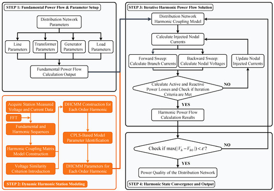
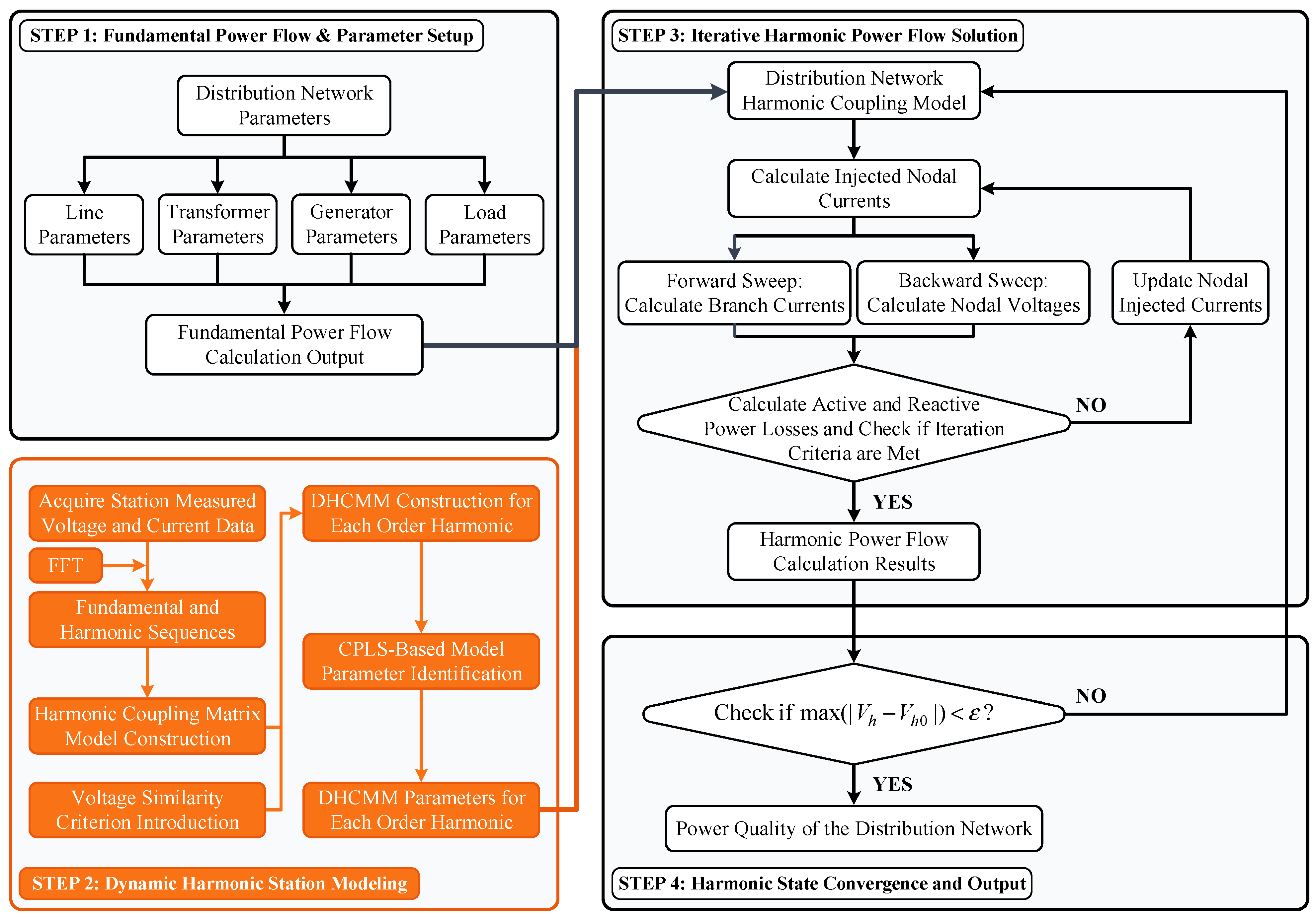
Figure 2 illustrates the overall harmonic power flow calculation procedure. To overcome the limitations of conventional methods, where harmonic source modeling is decoupled from power flow solution and fixed parameters cannot adapt to time-varying characteristics of bidirectional charging stations, this paper develops a closed-loop iterative mechanism that couples the DHCMM with harmonic power flow calculation. This enables the collaborative solution of dynamic harmonic source modeling and network-wide harmonic power flow.

Figure 2. Flowchart of harmonic power flow calculation with DHCMM.

During iteration, the DHCMM computes the injected harmonic currents of each order based on the current harmonic voltage at the station’s grid-connected node. These currents serve as node excitations for harmonic power flow. Based on the component harmonic equivalent models established in Section 3.1, the harmonic power flow is solved by the loop-current-based backward/forward sweep method to acquire the harmonic distribution of the entire network. The updated nodal harmonic voltages are fed back to the DHCMM, which discriminates the variations of operating conditions by means of the voltage similarity criterion. It keeps the model parameters constant under stable operating conditions and automatically reconstructs the harmonic coupling matrix to implement adaptive parameter updating when drastic operating condition changes (such as charging/discharging mode switching) occur. These two processes iterate until nodal harmonic voltages of the entire network reach convergence. The specific computational steps are detailed as follows.

• Step 1: Fundamental Power Flow Calculation

Based on the fundamental parameters of key equipment including generators, transmission lines, transformers, and loads, the Newton–Raphson method is employed to conduct the fundamental power flow calculation. This step yields the fundamental voltage and power distribution at each bus, serving as the initial conditions for subsequent harmonic analysis.

• Step 2: Construction of DHCMM for Charging Stations with Bidirectional Capability

Utilizing measured harmonic voltage and current data from the grid-connected nodes of the charging stations, the harmonic coupling relationships are fitted using the complex-domain least squares method to construct the HCMM. On this basis, considering the influence of operating state variations and voltage fluctuations, a dynamic updating mechanism for model parameters is implemented via a voltage similarity criterion. This establishes a DHCMM suitable for time-varying operating conditions.

• Step 3: Harmonic Power Flow Calculation

Given the fundamental voltages at each bus and the harmonic equivalent models of all system components, the DHCMM is integrated into the corresponding nodes as a harmonic source. A loop-current-based backward/forward sweep method is adopted to sequentially solve the nodal harmonic admittance equations for each harmonic order. Specifically, branch harmonic currents are calculated through the forward sweep, and nodal harmonic voltages are updated via the backward sweep. This iterative process continues until the steady-state harmonic distribution for the specific harmonic order is obtained. The procedure is repeated to cover all required harmonic orders.

• Step 4: Result Correction and Model Updating

The calculated harmonic voltage vector $U_h$ is compared with the voltage vector $U_{h0}$ from the previous iteration. If the convergence criterion $\max (|U_h-U_{h0}|)<\epsilon$ is satisfied, the harmonic power flow is deemed converged, and the final results are output. Otherwise, the parameters of the source and load harmonic models are updated based on the current harmonic voltage results. The process then returns to Step 3 to re-execute model construction and power flow calculation until convergence is achieved. The convergence criterion for harmonic power flow is explicitly set to 1 × 10⁻⁴. Under typical operating conditions, the proposed method converges within three to five iterations, which ensures high computational efficiency for dynamic harmonic analysis.

In the aforementioned process, if a significant change in the station’s operating state is detected, the dynamic updating mechanism of the DHCMM is triggered. The harmonic coupling matrix is then re-fitted to ensure consistency between the model and actual conditions, thereby enhancing the accuracy of the harmonic assessment.

4. Case Study

4.1. Field Measurement Data

The proposed model is validated using field measurement data from a bidirectional charging station in Wuxi City, Jiangsu Province, China [29,30,31]. This station is supplied by four 1250 kW transformers. Beneath transformers #1, #2, and #3, in addition to conventional charging piles and base loads, ten 60 kW bidirectional charging/V2G piles are connected to each transformer. Transformers #3 and #4 achieve a 380 V bus interconnection via a flexible interconnection device. Furthermore, a 36.48 kWp photovoltaic system and one 60 kW DC-supplied charging pile are integrated into the equipment’s 750 V DC bus. The bidirectional charging/V2G piles within this station have a rated power of 60 kW and a maximum DC charging and discharging current of 120 A. Power conversion is realized by paralleling four 15 kW conversion modules. The operating condition switching data of six electric vehicles were monitored at test point #1. The data acquisition system of this test adopts a high-precision data acquisition instrument (DEWE248) from Dewetron, Austria with the sampling frequency set to 50 kHz; the harmonic analysis time window length is 200 ms; and the voltage/current measurement accuracy class is 0.03. The primary test scenarios include the following with different observation periods for each scenario.

Scenario a: Six EVs switching from synchronous charging to synchronous discharging (with the switching action initiated at 0 s and observed until 753 s);

Scenario b: Initially six EVs charging with one switching to discharging (with the switching action initiated at 0 s and observed until 375 s);

Scenario c: Initially six EVs charging with two switching to discharging (with the switching action initiated at 0 s and observed until 503 s);

Scenario d: Initially six EVs discharging, switching to charging sequentially (one by one) (with the switching action initiated at 0 s and observed until 1131 s);

Scenario e: Initially six EVs charging, switching to discharging sequentially (one by one) (with the switching action initiated at 0 s and observed until 865 s);

Scenario f: Free charging/discharging transitions with three EVs charging and three EVs discharging (with the switching action initiated at 0 s and observed until 852 s).

These scenarios systematically cover typical operational modes, i.e., from synchronized group switching to gradual individual transitions, as well as mixed-mode operation, providing a comprehensive basis for validating the proposed DHCMM under both conventional unidirectional and bidirectional V2G conditions. The simulation model is developed in the MATLAB 2025a/Simulink environment, and the proposed method is compared with all approaches listed in Table 1 for validation. In addition, this paper adopts the Hanning window to conduct Fast Fourier Transform on various scenarios to suppress spectral leakage.

4.2. Validation of the DHCMM

4.2.1. Dynamic Harmonic Fitting Analysis

To verify the effectiveness of the proposed DHCMM under complex operating conditions, a fitting analysis of the harmonic currents was conducted using the measured data from the bidirectional charging station. The measured Phase-A voltage and current at the point of common coupling were selected as the analysis subjects.

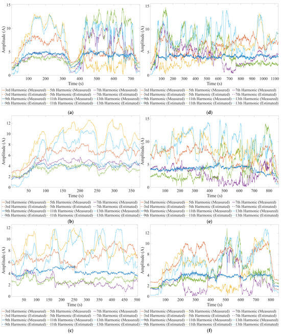
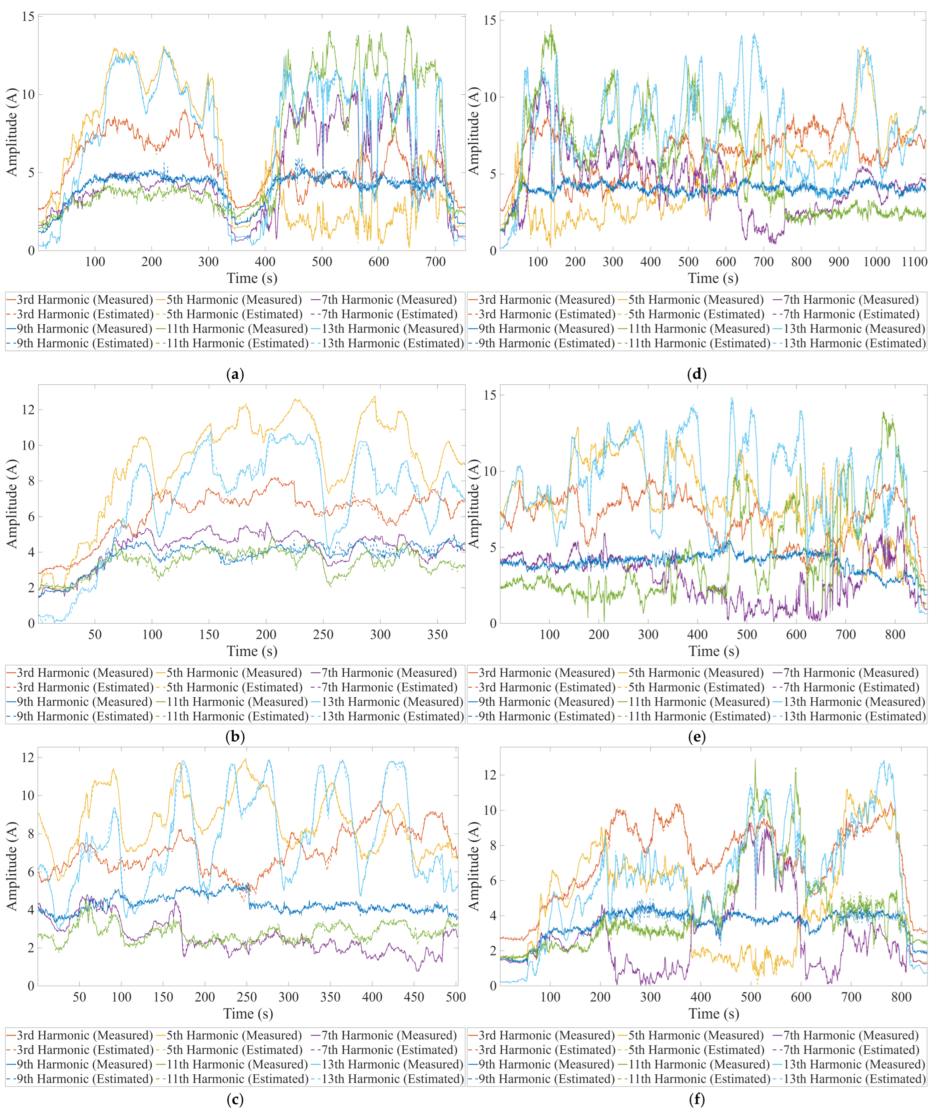
The relative errors between estimated and measured current amplitudes were calculated, and the model’s fitting accuracy across scenarios is presented in Table 2. The proposed model accurately estimates harmonic currents across all frequencies and scenarios. Furthermore, the fluctuation patterns of harmonic currents at different frequencies reveal distinct dynamic characteristics, as analyzed below for each scenario. Figure 3 compares the measured and estimated harmonic current waveforms.

Table 2. Root mean square error (RMSE) between the measured data and various harmonics fitted by the DHCMM under different scenarios.

Scenario	3rd Harmonic	5th Harmonic	7th Harmonic	9th Harmonic	11th Harmonic	13th Harmonic
a	1.69%	4.79%	3.32%	1.76%	1.52%	4.15%
b	2.62%	1.81%	2.49%	1.60%	2.21%	1.52%
c	2.52%	1.64%	2.87%	1.71%	2.64%	1.17%
d	1.76%	3.88%	2.99%	2.68%	3.19%	1.87%
e	1.41%	3.56%	4.79%	3.31%	3.53%	2.15%
f	1.33%	3.96%	4.57%	4.50%	3.88%	2.44%

Figure 3. Time-domain tracking performance of measured and estimated harmonic amplitudes based on DHCMM under different scenarios. (a) Harmonic current estimation under Scenario a; (b) harmonic current estimation under Scenario b; (c) harmonic current estimation under Scenario c; (d) harmonic current estimation under Scenario d; (e) harmonic current estimation under Scenario e; (f) harmonic current estimation under Scenario f.

As shown in Figure 3 and Table 2, in the synchronous switching condition of Scenario a, the 3rd harmonic achieves the best fit, while the 9th harmonic shows the largest error. Harmonic amplitudes diverge: the 3rd, 5th, 11th, and 13th harmonics are dominated by charging, whereas the 7th harmonic is dominated by discharging. The 13th harmonic experiences the maximum fluctuation amplitude. After switching to discharging, overall harmonic fluctuations stabilize with only the 7th harmonic maintaining highly dynamic.

In Scenarios b and c, where a subset of electric vehicles switches to discharging, all harmonic remains charging-dominated. The 5th harmonic shows the best fit, while the highest error occurs at the 9th or 11th harmonic shown in Figure 3b and Figure 3c, respectively. As the number of switched electric vehicles increases, dominant fluctuation frequencies shift from the 13th and 5th to the 11th and 13th with higher-order harmonics maintaining high fluctuation levels.

In the sequential switching scenarios, from discharging to charging Scenario d and from charging to discharging Scenario e, the 3rd harmonic yields the optimal fit in both cases. The 13th harmonic exhibits the highest error, though within 5%, and the strongest volatility. Switching direction affects dominance. When switching from discharging to charging, most harmonics are charging-dominated, while the 7th shows higher amplitude during the initial discharging stage. When switching from charging to discharging, all harmonics are charging-dominated, and the 5th amplitude is significantly higher than those of the 3rd and 7th. Following the sequential switching, overall harmonic fluctuations moderate, yet the 13th harmonic retains a high dynamic level.

In the free switching condition of Scenario f, the 3rd harmonic achieves the best fit, while the 7th harmonic has the highest error. The 13th harmonic amplitude continuously rises, showing the widest fluctuation range. The 5th harmonic amplitude is generally higher than that of the 3rd, whereas the 9th remains relatively stable. In the later stages of the free switching, overall fluctuations intensify with the 7th and 11th fluctuating significantly higher than that of the 3rd.

Across all six scenarios, the estimation error for each harmonic order remains within 5%, confirming that the DHCMM accurately captures the dynamic harmonic characteristics of bidirectional charging stations.

4.2.2. Comparative Analysis of Dynamic Modeling

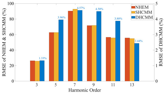
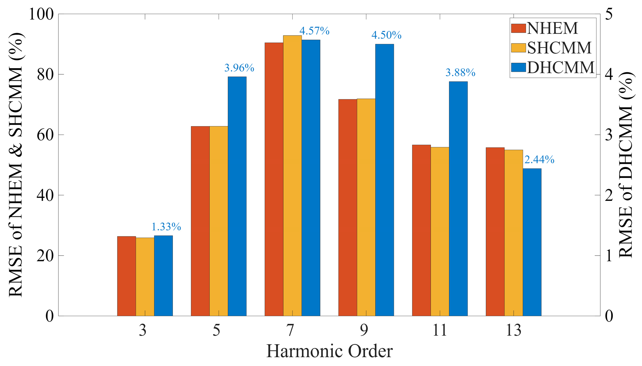
To further validate the DHCMM under operating condition switching, two representative categories, i.e., mechanism-based and data-driven, are selected for comparison. The mechanism-based models include an NHEM [32] and a trained SHCMM [33]. Using the free charging and discharging switching Scenario f as the test condition, Figure 4 compares the current amplitude-fitting deviations.

Figure 4. Comparison of the fitting results among different models.

As shown in Figure 4, both the NHEM and SHCMM exhibit high fitting errors across all frequencies. Because the NHEM neglects cross-coupling between harmonics, it cannot track dynamic operating conditions at all. The SHCMM, despite incorporating coupling, has fixed parameters and fails to adapt to condition changes, resulting in error levels comparable to NHEM. A purely static coupling model is inadequate for addressing the time-varying station characteristics.

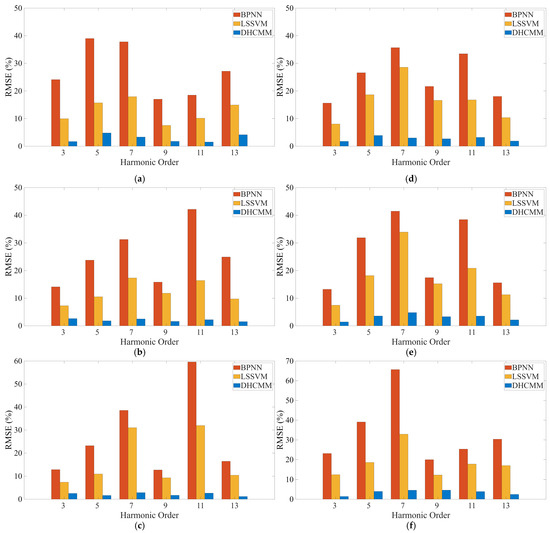
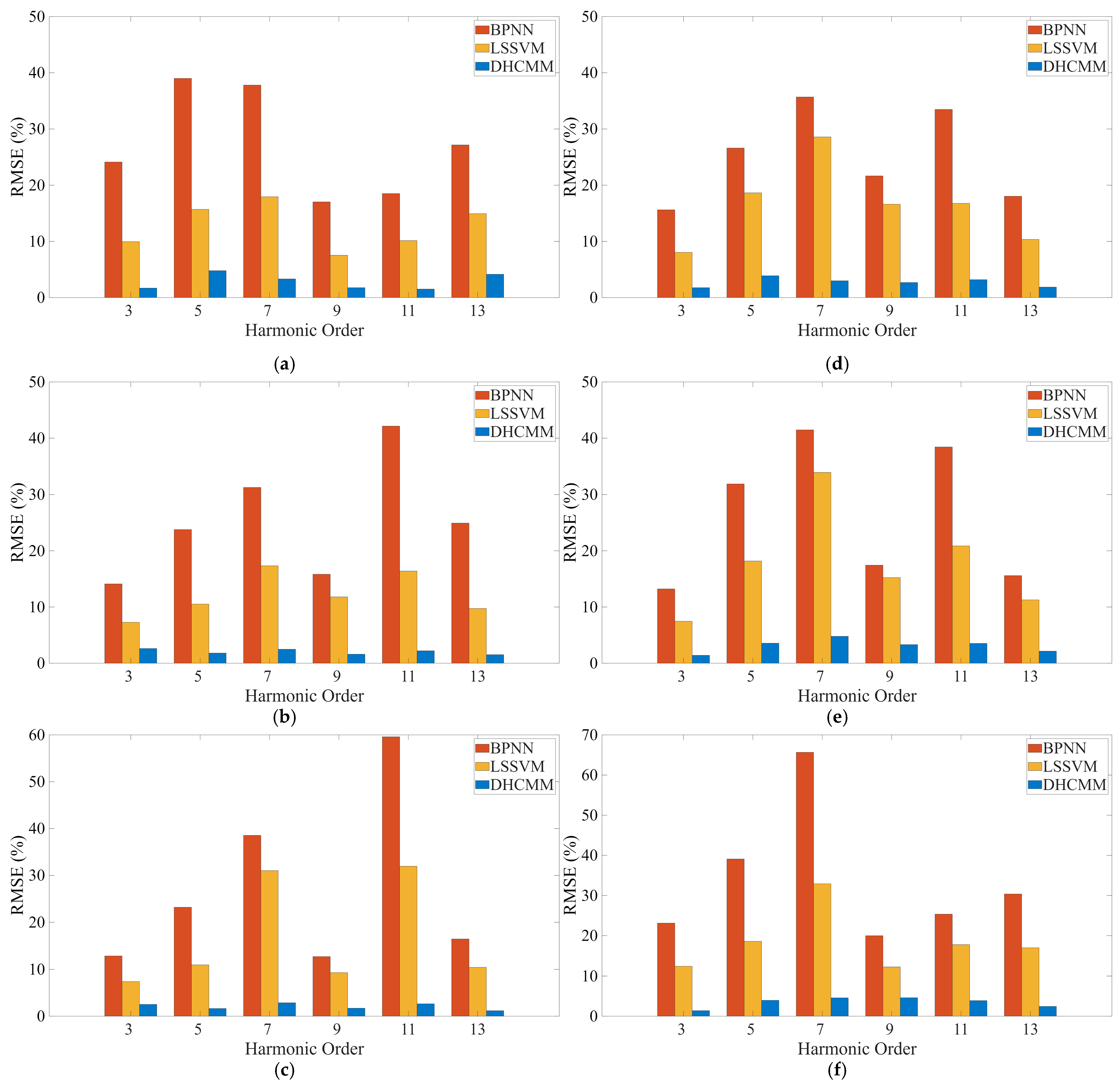
Regarding data-driven models, a BPNN [34] and an LS-SVM [35] are trained using the same data set. The sampling interval is 2 × 10⁻⁵ s, yielding approximately 50 million voltage and current data points under each scenario. The data set is split into training and test sets at a ratio of 2:8. For a BPNN, a single-hidden-layer feedforward neural network is adopted with 12 neurons for both the input and output layers and 40 neurons for the hidden layer. For an LS-SVM, individual fitting sub-models are constructed for the real and imaginary parts of each harmonic current. The model parameters are set as follows: penalty factor $\gamma =500$ and kernel function variance ${\sigma }^2=10$. Meanwhile, the MapMinMax normalization method is employed to map the sample features to the range of [−1, 1]. Figure 5 shows the RMSE results for all six scenarios.

Figure 5. RMSE comparison of DHCMM, BPNN and LS-SVM for harmonic fitting. (a) Harmonic fitting RMSE under Scenario a; (b) harmonic fitting RMSE under Scenario b; (c) harmonic fitting RMSE under Scenario c; (d) harmonic fitting RMSE under Scenario d; (e) harmonic fitting RMSE under Scenario e; (f) harmonic fitting RMSE under Scenario f.

As observed in Figure 5, although the BPNN and LS-SVM achieve better accuracy than static models, their inherent black-box nature prevents them from revealing the underlying physical mechanisms of harmonic coupling. Moreover, once trained, their parameters are fixed, making them unable to adapt to dynamic changes in operating conditions. Consequently, the overall error levels of these data-driven models remain significantly higher than the precision requirements for practical applications.

The proposed DHCMM demonstrates optimal performance. Its fitting errors are significantly lower in every harmonic comparison. Compared to the second-best performer here, i.e., the LS-SVM, the DHCMM reduces RMSE by approximately 6.88%, 12.16%, and 23.45% for the 3rd, 5th, and 7th harmonics, respectively. The DHCMM achieves RMSE below 5%, and the total harmonic current distortion estimation error for the bidirectional charging station is also within 5%.

Table 3 compares computational efficiency. Mechanism-based models, i.e., the NHEM and SHCMM, are the fastest due to their simple structures. Among data-driven models, the BPNN has the longest total computation time due to its large number of iterations, while the LS-SVM presents the highest average time per count as it needs to construct separate sub-models for each harmonic component. The proposed DHCMM achieves a total time of 292.8561 s, which is significantly lower than that of the BPNN, and an average time per iteration of 0.6026 s, which outperforms the LS-SVM.

Table 3. Comparison of computational efficiency for different harmonic modeling methods.

Method	Count Definition	Count	Total Computation Time (s)	Average Time Per Count (s)
DHCMM	Iterations	486	292.8561	0.6026
NHEM	Model Count	6	0.0202	0.0034
SHCMM	Model Count	6	0.0165	0.0034
BPNN	Iterations	1009	529.4290	0.5247
LS-SVM	Model Count	12	9.5462	0.7955

Thus, for charging stations undergoing EV charging/discharging mode transitions, the DHCMM effectively enhances harmonic evaluation accuracy while reducing the computational burden of frequent model updates.

4.2.3. Weight Coefficient Analysis

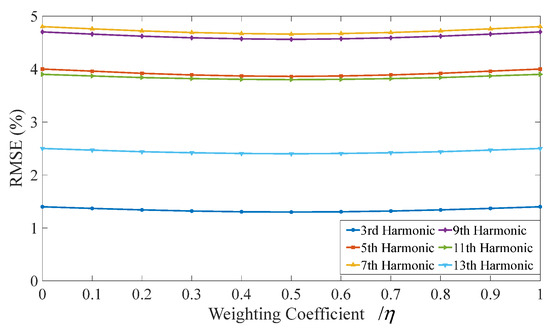
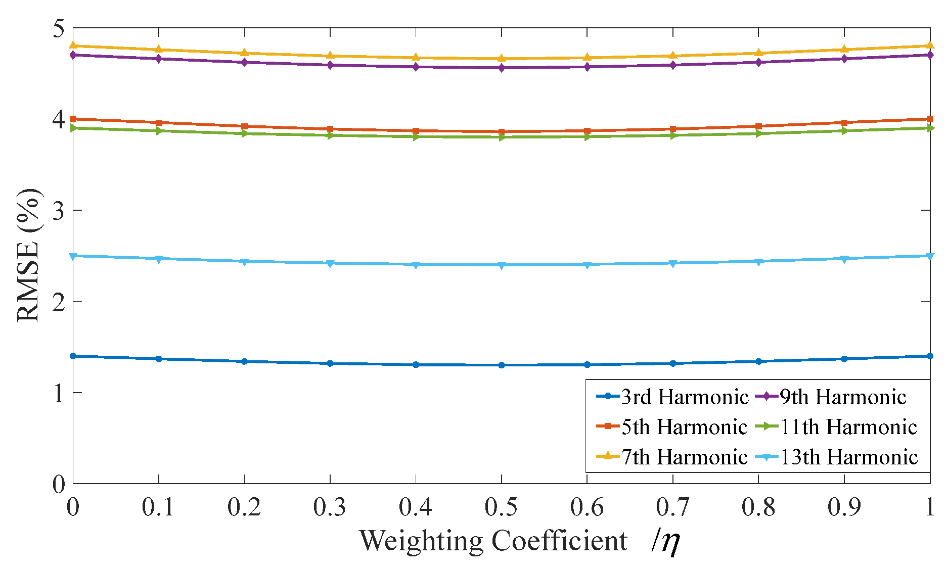
The weight coefficient $\eta$ in (12) balances amplitude similarity and phase similarity in the voltage similarity index. To assess its influence, sensitivity analysis is performed for $\eta \in [0.1,0.2,0.3,0.4,0.5,0.6,0.7,0.8,0.9]$. Figure 6 plots the harmonic tracking error and update trigger frequency against $\eta$. The average error reaches its minimum when $\eta =0.5$. Therefore, we selected $\eta =0.5$ as the weight coefficient.

Figure 6. RMSE of DHCMM harmonics under different weight coefficients.

4.3. Harmonic Power Flow Analysis of Distribution Network with Grid-Connected Stations

To simulate the power quality impacts of the grid-connected charging stations with bidirectional capability on the distribution network, the proposed DHCMM, which has been validated using field measurement data in Section 4.2, is employed as the harmonic source model. The voltage fluctuations and harmonic distortion rates at various buses within the distribution network are analyzed using the harmonic power flow calculation method described in Section 3. Since field measurement data at the distribution network level are difficult to obtain, the standard IEEE 33-bus distribution system is adapted as a representative test case to enable a controlled and reproducible analysis of the harmonic propagation characteristics.

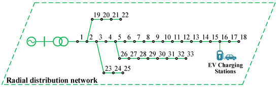
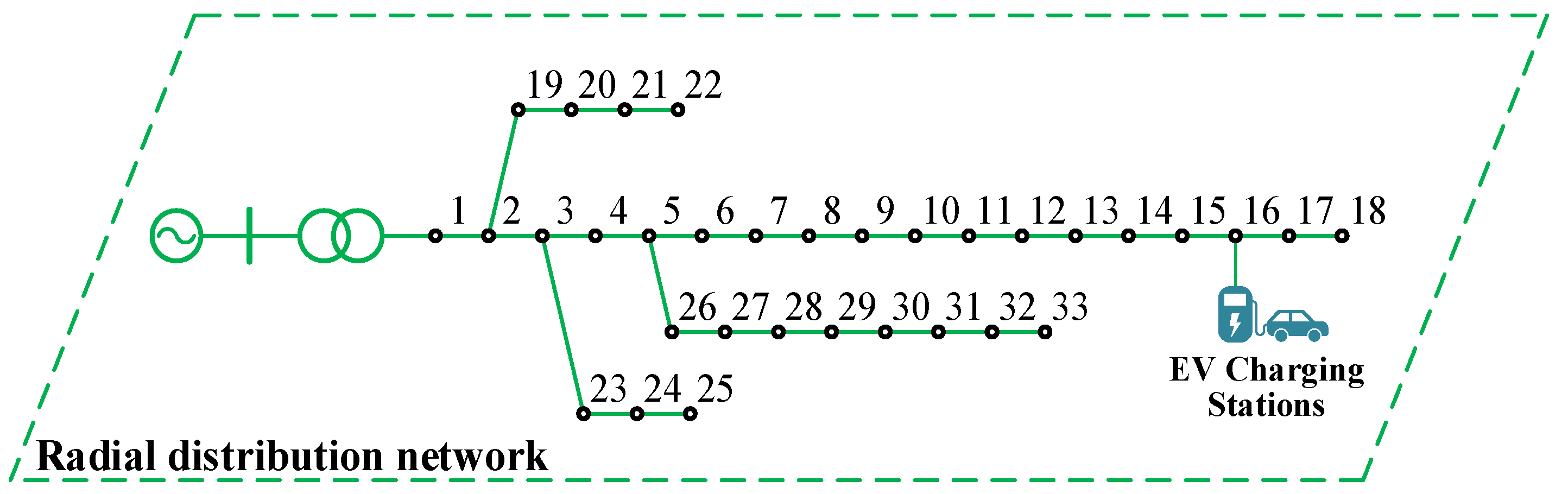
The IEEE 33-bus system has a rated voltage of 12.66 kV. In this system, Bus 1 serves as the slack bus with a voltage of 1.0 p.u., while all other buses operate as load buses. Bus 16, where the charging station is connected, acts as the harmonic current injection bus. The topological structure of the system is illustrated in Figure 7.

Figure 7. Topology of the IEEE 33-bus system with grid-connected station.

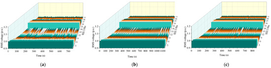
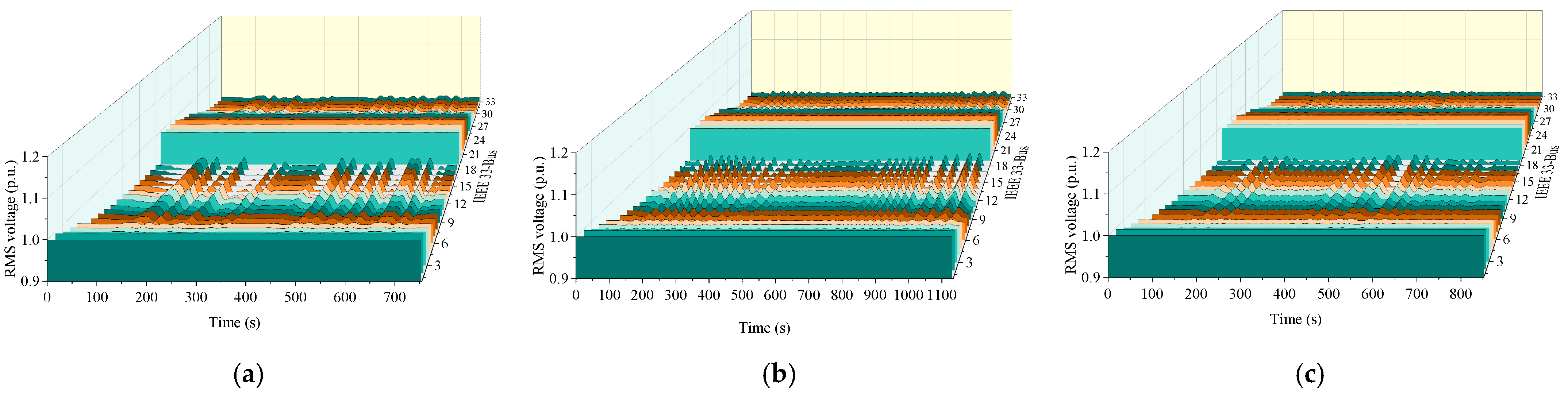
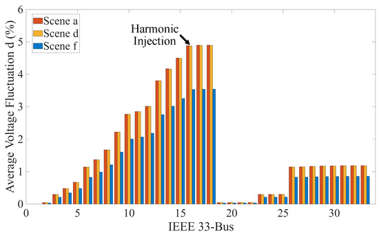
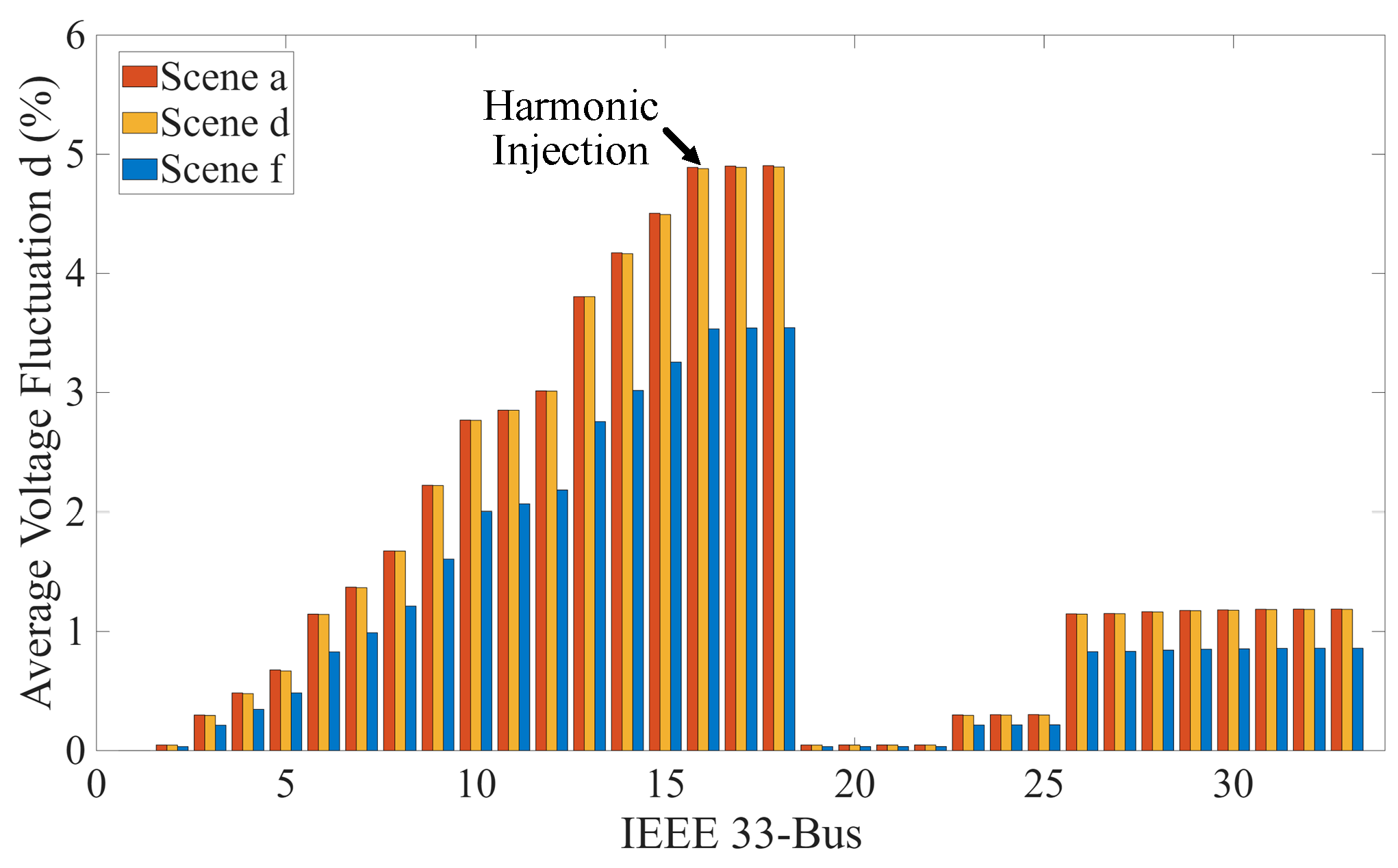
The dynamic harmonic coupling matrices fitted from the measured data of Scenarios (a), (d), and (f) are incorporated into Bus 16 of the IEEE 33-bus system. Using the harmonic power flow calculation method, the three-dimensional voltage waveform diagrams of all bus nodes in the system under different scenarios are obtained, as shown in Figure 8. Based on the voltage per-unit values of each node, the voltage fluctuation comparison diagrams at each node under different scenarios are derived using the calculation formula for voltage fluctuation ($d=(U_{\max }-U_{\min })\times 100\%$), as shown in Figure 9.

Figure 8. Voltage fluctuations of power system nodes under harmonic injection in different scenarios. (a) Voltage waveform under Scenario a; (b) voltage waveform under Scenario d; (c) voltage waveform under Scenario f.

Figure 9. Voltage fluctuation magnitudes at each bus under different scenarios.

The simulation results indicate that following the integration of the DHCMM, both the voltage distortion rates and voltage fluctuation magnitudes at Bus 16, i.e., the station bus, and its adjacent buses increase significantly, whereas buses farther from the station experience relatively minor impacts. The voltage fluctuation estimation error across all buses remains within 5% as well. These findings confirm that the grid integration of bidirectional charging stations affects power quality not only at the local bus but also in neighboring regions.

5. Conclusions

To handle complex operating conditions and time-varying harmonics in bidirectional charging stations, this paper proposes a DHCMM approach. Validation using field measurement data from a real-world station under six typical scenarios, the DHCMM provides accurate harmonic modeling with both the total harmonic current distortion estimation error and the voltage fluctuation estimation error within 5%. Compared with mainstream methods, including the Norton equivalent model, the SHCMM, the BPNN, and the LS-SVM, the proposed DHCMM demonstrates higher fitting accuracy.

Integrating the DHCMM as a harmonic source into the IEEE 33-bus system for harmonic power flow analysis reveals that the grid connection of the station not only significantly increases the voltage distortion rates and fluctuation levels at its local bus but also degrades power quality to adjacent buses. These results confirm the effectiveness and engineering practicality of the proposed method for assessing power quality impacts.

The proposed DHCMM distinguishes itself from existing methods by integrating a voltage-similarity-based adaptive updating mechanism into a harmonic coupling matrix framework. This hybrid mechanism-data-driven design avoids the static limitations of conventional mechanism-based models and the heavy data dependence of black-box data-driven models, achieving accurate and computationally efficient harmonic tracking under dynamic charging/discharging mode switching. For three-phase unbalanced systems, the DHCMM can be extended by constructing a separate harmonic coupling matrix for each phase or by forming a full three-phase block matrix without altering the dynamic updating mechanism.

A current limitation is that synchronous field measurements across multiple stations are not yet available due to high costs and long coordination cycles. Moreover, the harmonic power flow analysis was performed on an IEEE test feeder rather than an actual distribution network.

Future work includes establishing a multi-station experimental platform with diverse geographic and load characteristics to validate and enhance generalization. Additionally, we will extend the DHCMM to three-phase unbalanced systems and incorporate probabilistic harmonic power flow analysis to account for stochastic EV behaviors and renewable energy fluctuations. This will support the development of adaptive harmonic mitigation strategies, providing theoretical and technical foundations for a safe and efficient grid integration of large-scale bidirectional charging stations.

References

- Yang, X.L.; Deng, C.H.; Liu, G.G.; Huang, W.T.; He, J.; Zhu, L.W. Expansion Planning of Electric Vehicle Charging Stations Considering the Benefits of Peak-Regulation Frequency Modulation. IET Gener. Transm. Distrib. 2022, 16, 1400–1415. [Google Scholar] [CrossRef] [Scilit]
- Letcher, M.; Britton, J. The role of Electric Vehicle-to-X in Net Zero Energy Systems: A Comprehensive Review. Energy Res. Soc. Sci. 2025, 122, 104021. [Google Scholar] [CrossRef] [Scilit]
- Kettner, A.M.; Reyes-Chamorro, L.; Becker, J.K.M.; Zou, Z.X.; Liserre, M.; Paolone, M. Harmonic Power-Flow Study of Polyphase Grids with Converter-Interfaced Distributed Energy Resources-Part I: Modeling Framework and Algorithm. IEEE Trans. Smart Grid 2022, 13, 458–469. [Google Scholar] [CrossRef] [Scilit]
- Alfalahi, S.T.Y.; Alkahtani, A.A.; Al-Shetwi, A.Q.; Al-Ogaili, A.S.; Abbood, A.A.; Mansor, M.B.; Fazea, Y. Supraharmonics in Power Grid: Identification, Standards, and Measurement Techniques. IEEE Access 2021, 9, 103677–103690. [Google Scholar] [CrossRef] [Scilit]
- Milovanovic, M.; Radosavljevic, J.; Perovic, B. A Backward/forward sweep Power Flow Method for Harmonic Polluted Radial Distribution Systems with Distributed Generation Units. Int. Trans. Electr. Energy Syst. 2020, 30, 12310. [Google Scholar] [CrossRef] [Scilit]
- Zhu, S.; Liu, J.; Cao, Y.; Guan, B.; Du, X. Vienna Rectifier Modeling and Harmonic Coupling Analysis Based on Harmonic State-Space. Electronics 2024, 13, 1447. [Google Scholar] [CrossRef] [Scilit]
- Amry, Y.; Elbouchikhi, E.; Le Gall, F.; Ghogho, M.; El Hani, S. Electric Vehicle Traction Drives and Charging Station Power Electronics: Current Status and Challenges. Energies 2022, 15, 6037. [Google Scholar] [CrossRef] [Scilit]
- Wang, X.; Blaabjerg, F. Harmonic Stability in Power Electronic-Based Power Systems: Concept, Modeling, and Analysis. IEEE Trans. Smart Grid 2019, 10, 2858–2870. [Google Scholar] [CrossRef] [Scilit]
- Kettner, A.M.; Paolone, M. On the Properties of the Compound Nodal Admittance Matrix of Polyphase Power Systems. IEEE Trans. Power Syst. 2019, 34, 444–453. [Google Scholar] [CrossRef] [Scilit]
- Li, C.; Lu, W.; Xie, H.; Tao, J.; Chen, P.; Chen, X.; Shang, X. Stability Analysis and Parameter Optimization of SVG in Renewable Energy Collection Stations Based Frequency-Domain Admittance Matrix. Front. Energy Res. 2026, 14, 1767966. [Google Scholar] [CrossRef] [Scilit]
- Li, S.; Mao, Y.; Zheng, Z. Harmonic Coupling Characteristics of Inverters with Dynamic Disturbances Based on Harmonic State Space. J. Power Electron. 2025, 25, 1403–1415. [Google Scholar] [CrossRef] [Scilit]
- Sakinci, O.C.; Lekić, A.; Beerten, J. Generalized Impedance-based AC/DC Power System Modeling for Harmonic Stability Analysis. Int. J. Electr. Power Energy Syst. 2022, 143, 108456. [Google Scholar] [CrossRef] [Scilit]
- Kwon, J.B.; Wang, X.F.; Blaabjerg, F.; Bak, C.L.; Sularea, V.S.; Busca, C. Harmonic Interaction Analysis in a Grid-Connected Converter Using Harmonic State-Space (HSS) Modeling. IEEE Trans. Power Electron. 2017, 32, 6823–6835. [Google Scholar] [CrossRef] [Scilit]
- Kwon, J.B.; Wang, X.F.; Blaabjerg, F.; Bak, C.L. Frequency-Domain Modeling and Simulation of DC Power Electronic Systems Using Harmonic State Space Method. IEEE Trans. Power Electron. 2017, 32, 1044–1055. [Google Scholar] [CrossRef] [Scilit]
- Balouji, E.; Salor, Ö.; McKelvey, T. Deep Learning Based Predictive Compensation of Flicker, Voltage Dips, Harmonics and Interharmonics in Electric Arc Furnaces. IEEE Trans. Ind. Appl. 2022, 58, 4214–4223. [Google Scholar] [CrossRef] [Scilit]
- Zheng, J.H.; Song, K.; Duan, J.Q.; Wang, Y. An Adaptive Multi-Task Gaussian Process Regression Approach for Harmonic Modeling of Aggregated Loads in High-Voltage Substations. Energies 2025, 18, 4670. [Google Scholar] [CrossRef] [Scilit]
- De Souza, L.A.A.; Martins, M.B.; Pinto, M.V.V.; Lima, A.C.S.; Moura Junior, N.N. Data-Driven Modeling of Nonlinear Transducers for Harmonic Measurements. IEEE Trans. Instrum. Meas. 2025, 74, 9529808. [Google Scholar] [CrossRef] [Scilit]
- Nduka, O.S.; Ahmadi, A.R. Data-driven Robust Extended Computer-Aided Harmonic Power Flow Analysis. IET Gener. Transm. Distrib. 2020, 14, 4398–4409. [Google Scholar] [CrossRef] [Scilit]
- Abbood, H.D.; Benigni, A. Data-Driven Modeling of a Commercial Photovoltaic Microinverter. Model. Simul. Eng. 2018, 11, 5280681. [Google Scholar] [CrossRef] [Scilit]
- Xie, X.M.; Chen, D.L. Data-driven Dynamic Harmonic Model for Modern Household Appliances. Appl. Energy 2022, 312, 118759. [Google Scholar] [CrossRef] [Scilit]
- Jiang, K.Z.; Hu, P.; Cao, K.; Liu, D.; Ye, C. Small-Signal Modeling and Interaction Analysis of LCC-HVDC Systems Based on Harmonic State Space Theory. IEEE Access 2022, 10, 109937–109948. [Google Scholar] [CrossRef] [Scilit]
- Salis, V.; Costabeber, A.; Cox, S.M.; Zanchetta, P. Stability Assessment of Power-Converter-Based AC systems by LTP Theory: Eigenvalue Analysis and Harmonic Impedance Estimation. IEEE J. Emerg. Sel. Top. Power Electron 2017, 5, 1513–1525. [Google Scholar] [CrossRef] [Scilit]
- Liu, W.; Lu, Z.X.; Wang, X.F.; Xie, X.R. Frequency-coupled Admittance Modelling of Grid-Connected Voltage Source Converters for the Stability Evaluation of Subsynchronous Interaction. IET Renew. Power Gener. 2019, 13, 285–295. [Google Scholar] [CrossRef] [Scilit]
- Yang, Y.H.; Wang, S.R.; Shi, M.M.; Zheng, X. A Piecewise Linearization Based Method for Crossed Frequency Admittance Matrix Model Calculation of Harmonic Sources. Sensors 2025, 25, 582. [Google Scholar] [CrossRef] [Scilit] [PubMed]
- Nan, L.; Wei, W. Analysis on the Improved Method of Nonlinear Load Norton Equivalent Model. J. Electron. Meas. Instrum. 2017, 31, 1336–1341. [Google Scholar] [CrossRef]
- Kim, W.-J.; Nam, S.-R.; Kang, S.-H. Adaptive Phasor Estimation Algorithm Based on a Least Squares Method. Energies 2019, 12, 1387. [Google Scholar] [CrossRef] [Scilit]
- Shi, B.J.; Xu, F. Improved Harmonic Current Detection Method in Recursive Least Square Algorithm. J. Shanghai Dianji Univ. 2018, 21, 43–46. [Google Scholar]
- Chen, C.I.; Chen, Y.C. A Neural-Network-Based Data-Driven Nonlinear Model on Time- and Frequency-Domain Voltage–Current Characterization for Power-Quality Study. IEEE Trans. Power Deliv. 2015, 30, 1577–1584. [Google Scholar] [CrossRef] [Scilit]
- China’s State Grid Opens Biggest Commercial Demonstration Area for Vehicle-to-Grid Technology. Available online: https://www.yicaiglobal.com/news/china-kicks-off-largest-v2g-zone-for-future-e-mobility (accessed on 27 May 2026).
- Initiating a Two-Way Era for Electric Vehicles and Power Grids. Available online: https://www.sdg-china.net/en/NewsList/info_itemid_71325.html (accessed on 27 May 2026).
- State Grid Wuxi Power Supply Company Showcases Innovative Achievements at the 2025 World Internet of Things Expo. Available online: https://news.cri.cn/20251105/42d26736-7e5d-f801-a998-8f0db30ff2ef.html (accessed on 27 May 2026).
- Singh, R.S.; Ćuk, V.; Cobben, S. Measurement-Based Distribution Grid Harmonic Impedance Models and Their Uncertainties. Energies 2020, 13, 4259. [Google Scholar] [CrossRef] [Scilit]
- Beites, L.F.; Mayordomo, J.G.; Yang, X. The Harmonically Coupled Admittance Matrix of the Single-Phase Diode Rectifier. IEEE Access 2021, 9, 128023–128031. [Google Scholar] [CrossRef] [Scilit]
- Yue, Q.Q.; Hu, R.; Zhang, X.L. A Power System Harmonic Problem Based on the BP Neural Network Learning Algorithm. Comput. Intell. Neurosci. 2022, 8, 7247881. [Google Scholar] [CrossRef] [Scilit] [PubMed]
- Kirinčić, V.; Čeperić, E.; Vlahinić, S.; Lerga, J. Support Vector Machine State Estimation. Appl. Artif. Intell. 2019, 33, 517–530. [Google Scholar] [CrossRef] [Scilit]
- Wu, W.; Li, J.; Mao, T.; Liu, S.; Zhou, B.; Zeng, D. Modeling and Analysis on AC-DC Harmonic Coupling of the Three-Phase Voltage Source Converter under Asymmetric Condition. Energies 2022, 15, 5466. [Google Scholar] [CrossRef] [Scilit]
Disclaimer/Publisher’s Note: The statements, opinions and data contained in all publications are solely those of the individual author(s) and contributor(s) and not of MDPI and/or the editor(s). MDPI and/or the editor(s) disclaim responsibility for any injury to people or property resulting from any ideas, methods, instructions or products referred to in the content. |
© 2026 by the authors. Licensee MDPI, Basel, Switzerland. This article is an open access article distributed under the terms and conditions of the Creative Commons Attribution (CC BY) license.