


Abstract
Hydrogen energy, owing to its advantages of low-carbon cleanliness, long-term storage capacity, and multi-energy coupling potential, has emerged as a crucial medium for enhancing renewable energy accommodation within integrated energy systems. However, the pronounced heterogeneity in hydrogen load behaviors, temporal characteristics, and regulation capabilities poses significant challenges for unified modeling approaches, which struggle to accurately capture the multi-modal regulation potential of hydrogen demand, thereby limiting the precision of system operation optimization. To address this issue, this paper proposes a data-driven hydrogen load flexibility modeling method for integrated energy system (IES) operation optimization. A hybrid LSTM-ISODATA framework is designed to extract deep temporal dependencies and identify six representative hydrogen consumption patterns from typical load sequences. Each hydrogen load category is decomposed into shiftable, transferable, and reducible flexible forms, and a category-specific time-varying flexibility constraint matrix is established to characterize differentiated regulation capabilities. An electricity–heat–hydrogen integrated energy system operation optimization model embedded with classified flexible hydrogen loads is developed and solved via mathematical programming. Simulation results show that the proposed method reduces system operating costs by 10.3% compared with conventional unified modeling, while significantly promoting renewable energy utilization and system operational flexibility. The effectiveness and engineering applicability of the proposed model in IES optimal scheduling are fully validated.
1. Introduction
In the context of the progressive depletion of conventional fossil energy, the proportion of renewable energy installed in the power system keeps growing and the coupling relationship between the power system and various energy carriers is increasingly close [1]. The integrated energy system formed by electricity–heat–hydrogen coupling provides an important way to alleviate the volatility of renewable energy and improve the flexibility of system operation by realizing energy conversion and coordinated scheduling among different energy carriers [2]. Unlike traditional energy carriers, hydrogen energy can be produced through electrolysis of water using surplus renewable energy, which not only solves the problem of abandoned wind and light but also achieves the clean production of energy. As an energy storage medium, hydrogen energy has a longer storage cycle and larger storage capacity compared with battery energy storage, and can realize cross-season energy storage, which effectively makes up for the deficiency of short-term energy storage technologies. In terms of connecting the power system and the terminal energy consumption side, hydrogen energy can be converted into electricity, heat and other forms according to the needs of terminal users, covering multiple fields such as industrial gas, transportation fuel, and residential heating, forming a closed loop of energy supply and consumption. Relevant research shows that hydrogen energy is characterized by its twofold role as an energy carrier and energy storage medium, and has unique advantages in connecting power system and terminal energy consumption side, and has been increasingly incorporated into IES modeling and operation studies [3,4,5].
However, compared with electric load and heat load, hydrogen load shows more significant heterogeneity in energy consumption behavior and operation characteristics. On the one hand, there are obvious differences in hydrogen scale, time distribution and continuity requirements in different hydrogen scenarios. On the other hand, the adjustable ability of hydrogen load is subject to the hydrogen production mode, storage, and transportation conditions and terminal hydrogen process, and its flexible characteristics have strong imbalance in time scale and adjustment mode. Based on the operational characteristics of hydrogen energy system, the feasibility of hydrogen load participating was analyzed in [6,7], which is scheduling from the perspective of operation mechanism and economy of electrolytic hydrogen production, and pointed out that its regulation ability was significantly affected by equipment operation constraints. A risk-aware scheduling model for an electricity–gas–hydrogen integrated energy system was developed by incorporating dynamic electrolyzer modeling, hydrogen blending into gas networks, and spectral risk theory in [8], showing that diversified hydrogen utilization can enhance system economy and renewable energy accommodation. Based on the improved energy system model, the role of hydrogen energy in different roles was systematically evaluated in [9], such as terminal energy consumption, energy conversion, and power chemical energy storage.
Aiming at the problem of load-side heterogeneity of IES, a multitude of scholars have engaged in studies on load regulation potential boundary identification and demand-side resource fine scheduling method in recent years. By constructing the operation optimization model of hydrogen-containing integrated energy system, the cooperative operation mechanism between hydrogen energy storage, hydrogen production load, and renewable energy was analyzed in [10,11], and the impact of trans-energy carrier regulation on system economy was revealed. At the same time, demand response and flexible load modeling methods are gradually introduced into the research of integrated energy systems. The load flexibility was abstracted into a translatable, reducible, or transferable form in [12,13,14,15], and incorporated it into the scheduling model by preset proportional parameters to achieve a unified description of the load-side regulation capability.
In order to improve the ability to describe load heterogeneity, data-driven methods have been gradually introduced into the field of load analysis and modeling. By exploiting large-scale historical operation data, clustering algorithms and time-series feature extraction techniques have been employed to identify representative load behavior patterns and distinguish different consumption modes. The load operation characteristics were classified in [16,17] through cluster analysis and temporal feature extraction, providing a new perspective for differentiated flexible load modeling. Furthermore, the integration of load behavior classification results with the constraint structure of scheduling models was investigated in [18], enabling data-driven load characteristics to be embedded into operation optimization frameworks. Beyond clustering-based approaches, advanced spatiotemporal representation learning and forecasting methods have been widely applied to characterize the intermittency and stochastic nature of renewable generation and load dynamics. For example, embedded graph structure learning and trend categorization were developed in [19,20] to capture complex spatial–temporal correlations in wind farm clusters, while fluctuation classification and probabilistic prediction techniques were proposed in [21] to describe different photovoltaic output patterns and their uncertainty characteristics. More recently, Caminiti et al. [22] introduced a GIS-based method that maps pollutant emissions and traffic volumes onto the road network to produce municipal-level mobility-impact indexes, demonstrating that integrating spatial data with mobility patterns can effectively quantify the heterogeneous environmental benefits of transport electrification and reveal non-linear urbanization–benefit relationships. These studies demonstrate that data-driven temporal representation learning is effective in extracting behavioral features from energy-related time-series data and provides important support for differentiated modeling and uncertainty-aware operation of integrated energy systems. However, existing data-driven load analysis and flexible modeling research mainly focuses on electrical or thermal loads, and studies on hydrogen load behavior modeling remain at an early stage. At present, most works simplify hydrogen loads as fixed or proportionally adjustable demands, or directly adopt flexible modeling approaches developed for electrical and thermal loads. Such treatments fail to accurately reflect the fundamental differences in continuity constraints and adjustment potential among various hydrogen usage scenarios, which limits the effectiveness of hydrogen load participation in IES operation optimization [23]. Several works have begun to explore data-driven characterization of hydrogen-related demand. Hydrogen refueling operations were explicitly simulated to generate representative hydrogen load profiles, and clustering was applied to obtain typical demand patterns for integrated hydrogen system planning [24]. Hydrogen-load demand-side response has also been modeled in day-ahead scheduling for renewable-powered hydrogen production systems, demonstrating that hydrogen demand can be treated as an actively adjustable load under time-varying electricity prices rather than a purely exogenous requirement [25]. These studies indicate that data-driven hydrogen load profiling and demand response modeling can provide a quantitative basis for describing heterogeneity and operational flexibility. More recently, supply–demand side flexibility has been jointly modeled within IES scheduling frameworks, where demand response and flexible resource dispatch are coordinated to improve renewable utilization and reduce operating cost [26]. In addition, the incorporation of comprehensive electrolyzer operational characteristics and sophisticated multidimensional demand response mechanisms have been incorporated into electricity–hydrogen–heat integrated energy system scheduling, highlighting the importance of representing both device-level flexibility and user-side adaptability in optimization models [27].
Although recent data-driven studies have advanced load behavior analysis—such as clustering-based pattern identification [16,17,18] and spatiotemporal representation learning for renewable forecasting [19,20,21]—these efforts have predominantly focused on electrical and thermal loads. For hydrogen loads, existing works have begun to explore data-driven profiling [24] and demand-side response [25], yet they still largely treat hydrogen demand as either fixed, proportionally adjustable, or directly adopt flexibility models developed for electrical loads [23]. As a result, two critical gaps remain. On the one hand, there is a lack of systematic method to link hydrogen load classification results with the constraint structure of the scheduling model, despite the successful application of clustering to electrical load pattern grouping [16,17] and time-series clustering to demand response frameworks [18]. This disconnect prevents the intrinsic differences in continuity, interruptibility, and time-shiftability among various hydrogen usage scenarios from being accurately reflected in optimization models. On the other hand, unlike the rich body of work on differentiated electrical/thermal load flexibility [12,13,14,15], hydrogen demand continues to be treated as a homogeneous load or modeled using unified proportional flexibility parameters, whose adjustment ranges and cost coefficients are often empirically set without accounting for temporal or behavioral heterogeneity. This weakens the supporting role of flexible resources in system operation optimization to a certain extent.
To overcome this limitation, this paper introduces a behavior-driven methodology for modeling hydrogen load flexibility. In contrast to conventional models that apply a single proportional adjustment coefficient uniformly to all hydrogen demand, the proposed method employs data-driven clustering to classify hydrogen load behaviors into distinct categories. Each category is then assigned its own time-varying flexibility constraints, including shiftable, transferable, and reducible components. This distinction is critical because conventional uniform flexibility models implicitly assume that all hydrogen demand can be adjusted to the same degree at any time, which contradicts the operational reality: industrial continuous loads, transportation loads, and standby emergency loads have fundamentally different continuity requirements and adjustment tolerances. The proposed approach respects these differences and translates them into category-specific constraint matrices, as summarized in Table 1. Consequently, this new modeling framework not only enhances the physical interpretability of hydrogen load flexibility but also enables its direct integration into the optimization model of integrated energy systems. As quantified in Section 5, the proposed method achieves superior coordination with renewable energy generation and yields measurable cost reductions compared with conventional uniform flexibility representations. An optimization model for an electricity–heat–hydrogen integrated energy system is then formulated incorporating these differentiated hydrogen load flexibility constraints.
Table 1.
Comparison between conventional uniform flexibility modeling and the proposed classification-based flexibility modeling.
The main contributions of this paper are summarized as follows:
(1) Proposes a behavior-based modeling approach for hydrogen load flexibility. In traditional integrated energy system models, hydrogen demand is typically represented by fixed or proportional flexibility parameters, failing to capture the operational differences across various hydrogen application scenarios. This study characterizes hydrogen load flexibility through the time-varying features of load behavior processes, explicitly reflecting the spatiotemporal coupling and continuity characteristics of hydrogen demand. Compared with traditional unified flexibility modeling, this approach breaks through the limitation of homogeneous assumption and achieves the refined description of hydrogen load flexibility.
(2) Develops a data-driven clustering method integrating LSTM and ISODATA algorithms to identify typical hydrogen consumption patterns from typical time-series data. Compared with K-means and hierarchical clustering, the proposed L-ISODATA method can automatically optimize cluster number and suppress noise, which is more suitable for dynamic hydrogen load data. By correlating extracted load categories with differentiated flexibility, this approach incorporates the heterogeneity of hydrogen demand into modeling rather than simplifying it to a uniform adjustment parameter.
(3) Develop an operation optimization model for integrated power–heat–hydrogen systems based on the flexible hydrogen load model. By incorporating the adjustable characteristics of flexible hydrogen loads with diverse behaviors into the dispatch model, hydrogen demand can participate in system regulation in a manner consistent with its operational properties. This enhances the utilization rate of flexible resources and strengthens synergies with renewable energy sources.
2. Integrated Energy System Modeling
2.1. IES Architecture
Figure 1 presents the structural composition of the IES, which is mainly composed of energy supply side, coupling unit, energy storage unit, and load side. The supply-side components consist of wind turbine (WT), photovoltaic (PV), and power grid (PG). Power to hydrogen (P2H), hydrogen-fired turbine (HFT), fuel cell (FC) with characteristics of combined heat and power generation, absorption refrigeration (AR), and gas boiler (GB) capable of hydrogen combustion constitute an electro-hydrogen–heat coupling unit. The energy storage unit consists of electric energy storage (EES), thermal energy storage (TES), and hydrogen energy storage (HES). The load side is composed of electric load (EL), multi-type hydrogen load (HL), and heat and cold load (HCL).
Figure 1.
IES structure diagram.
The output of power source, hydrogen source, and heat source in the IES operates under the principle of prioritizing local load satisfaction. For the process of power supply and demand balance, when the load is low, there is excess output of wind power or photovoltaic power or surplus power in the upper power grid. The electrolytic cell uses excess power to produce hydrogen. Considering the adjustable characteristics of hydrogen loads, the system can then rationally allocate the storage and transportation of hydrogen energy. When the load is at the peak, there is a shortage of electric energy. The hydrogen storage tank and the hydrogen refueling station transport hydrogen to the IES, and cooperate with the hydrogen-fired turbine to generate electricity to make up for the shortage of electricity. For the hydrogen energy supply–demand balancing process, water electrolysis-based hydrogen production is first adopted to satisfy the requirements of hydrogen loads. When hydrogen is in surplus, it can be consumed by hydrogen-fired turbines to generate electricity and heat, and the recovered heat can be supplied to cold and heat loads through cogeneration systems and absorption chillers. Make full use of renewable energy while reducing operating costs. The introduction of hydrogen-fired turbines enables the efficient co-generation of electricity and heat from hydrogen, and achieve the cogeneration of heat and power of the system. The complementarity between its operational characteristics and the volatility of renewables results in markedly improved system stability and energy utilization efficiency.
2.2. Hydrogen Load Clustering Model Based on L-ISODATA
In contrast to traditional clustering methods that rely solely on static features, the proposed L-ISODATA framework captures both temporal dependencies and behavioral heterogeneity in hydrogen load; this enables a physically meaningful classification that directly supports differentiated scheduling strategies while enhancing model robustness and generalization across diverse operational scenarios. The hydrogen load classification process based on L-ISODATA is shown in Figure 2.
Figure 2.
Hydrogen load classification process based on L-ISODATA.
2.2.1. Temporal Feature Extraction Based on LSTM
Hydrogen load data exhibit strong temporal dependency and operational continuity, which are difficult to characterize using conventional statistical features. To capture these characteristics, the Long Short-Term Memory (LSTM) network was employed as a temporal feature encoder. The LSTM network was used as a temporal feature encoder to capture the sequential characteristics of hydrogen load, which is used to extract high-dimensional dynamic features from hydrogen load time series to characterize the time series dependence and evolution mode of different hydrogen consumption behaviors.
Given the hydrogen load time series xt, the LSTM updates its internal states as follows:
where is the input gate output at time t; is the input at time t; is the hidden state from the previous time step; and are weight matrices for the input and hidden state, respectively; is the bias term; ơ is the sigmoid activation function; is the forget gate output at time t; and are the weight matrices for the input and hidden state, respectively; is the bias term; is the output gate at time t; and are the weight matrices for the input and hidden state, respectively; is the bias term; is the cell state at time t; is the forget gate at time t; is the previous cell state; is the input gate; tanh is the hyperbolic tangent activation function; , , and are the weight matrices and bias term for the cell state; is the hidden state at time t.
The LSTM architecture adopted in this study consists of two stacked LSTM layers, each containing 64 memory cells. The first LSTM layer processes the input sequence and returns the full output sequence to the second layer, while the second LSTM layer outputs the final hidden state as the temporal feature vector. A dropout layer with a rate of 0.2 was applied after each LSTM layer to prevent overfitting. The input sequence length was set to 24 h, corresponding to one day of hourly hydrogen load data. The output dimension of the LSTM encoder was 64, which serves as the feature input to the subsequent ISODATA clustering algorithm.
The model was trained using the Adam optimizer with a learning rate of 0.001, a batch size of 32, and a maximum of 200 epochs. Early stopping with a patience of 10 epochs was applied based on validation loss. The mean squared error was used as the loss function. The training/validation split was 80%/20% of the one-year hourly dataset.
LSTM’s ability to model long-range dependencies in hydrogen load data is crucial for identifying underlying consumption patterns. The temporal features extracted by the LSTM network serve as the foundation for clustering hydrogen load behaviors.
2.2.2. Load Pattern Identification Using ISODATA Clustering
The temporal features extracted by the LSTM are further processed using the ISODATA clustering algorithm to identify typical hydrogen consumption patterns. ISODATA is an unsupervised clustering algorithm that iteratively refines cluster centers and adjusts the assignment of data points. ISODATA is an advanced variant of the K-means algorithm that is capable of handling high-dimensional and dynamic load data. It automatically optimizes the number of clusters online by merging similar clusters and splitting discrete clusters, thereby adapting to seasonal fluctuations in power load. By introducing the minimum cluster size threshold to filter the abnormal load, the anti-noise ability of the model is enhanced and the stability of the model is improved. The parameter constraints guide the merging and splitting of clusters, improve the accuracy of classification results, and are more in line with the actual load conditions.
The update rule for the ISODATA algorithm is expressed by:
where is the cluster center for cluster k; represents the set of samples assigned to cluster k; is the number of samples in cluster k; represents the feature vectors extracted by LSTM.
The ISODATA algorithm iterates until convergence, optimizing the cluster centers and sample assignments. This process groups similar hydrogen consumption behaviors into categories, which represent the main types of hydrogen demand behavior.
To evaluate the clustering quality, the Davies–Bouldin Index (DBI) and Dunn Index (DI) were employed to assess the quality of clustering from different perspectives. After the clustering results were output, the DBI index and the DI index were jointly utilized to assess the clustering effect. The formulas of DBI index and DI index are as follows:
where and are the average distance from the sample to the cluster center in the i and j clusters, respectively; is the distance between two cluster centers and ; is the maximum distance between samples in the cluster.
The DBI index evaluates the clustering quality by measuring the intra-class compactness and the inter-class separation , which can reflect the overall compactness and separation of the clustering structure. A smaller DBI indicates greater intra-cluster compactness and larger inter-cluster separation, thereby reflecting a superior clustering effect. The DI index focuses on the ratio of the minimum inter-class distance to the maximum intra-class distance . A larger DI indicates superior inter-cluster separation and intra-cluster compactness, thereby reflecting a better clustering effect. Overall, a lower DBI signifies better clustering by minimizing intra-cluster scatter relative to inter-cluster distance. Conversely, a higher DI reflects clearer separation, as it maximizes the ratio of the smallest inter-cluster distance to the largest intra-cluster diameter.
From an operational perspective, the clustering results remain meaningful because the identified hydrogen load categories present distinct dominant temporal behaviors and continuity characteristics, which are subsequently mapped to category-dependent flexibility constraints in the optimization model. Therefore, the DBI and DI results jointly support the statistical compactness and practical interpretability of the hydrogen load classification. Through the above L-ISODATA clustering model, the hydrogen load types with similar hydrogen consumption behavior patterns can be identified, which provides a basis for the subsequent construction of classified flexible characteristic model and differentiated scheduling strategy.
3. Flexible Hydrogen Load Modeling
The hydrogen load in the IES consists of basic load and flexible load. Under the premise of fine classification and aggregation of hydrogen load, the flexibility of load is not a unified attribute, but is determined by the physical characteristics and energy consumption behavior of different energy carriers. There are significant differences in continuity, timing adjustability, and interrupt tolerance among different hydrogen scenarios. Based on the clustering results of multi-type hydrogen load, this paper introduces a flexible modeling method of hydrogen load parameterized by load type to construct a unified and differentiated flexible load model.
3.1. Unified Modeling of Load Flexibility
Based on their response characteristics, flexible load can be categorized as shiftable, transferable, and reducible.
(1) Shiftable load
The shiftable load is characterized by the ability to shift its entire energy supply period, with the constraint that both the power level and the total duration of operation are predetermined and unchanged. It is uninterruptable, and the shift needs to be continuously run to completion within a period of time acceptable to the user. It is assumed that the shiftable interval is in the scheduling period:
where is the power of shiftable load in t period; is the proportion of shiftable load; is the rated power of shiftable load; is a set of shiftable starting periods; is the duration of shiftable load.
(2) Transferable load
Transferable loads are defined as loads for which power consumption can be flexibly shifted among specific time intervals during the full scheduling cycle, with total energy usage unchanged. Compared with the shiftable load, there is no limitation of continuity and timing, and it has high time elasticity. In order to prevent frequent start and stop of the equipment, the constraints on the transfer power and the minimum continuous transfer time of the transferable load are established as follows:
where is the state of transferable load; is the transferred power at time t; and are the upper and lower limits of the transferred power; is the minimum time for continuous operation of the equipment.
(3) Reduced load
A load capable of reduction refers to the load that the power supply can be adjusted during a specific period of time. To guarantee the rationality of load reduction, the constraints on the number and duration of load reduction are as follows:
where is the power at time t after load dispatch that can be reduced; is the state of load reduction at time t; is the proportion of load that can be reduced; is the rated power of load reduction; and are the minimum and maximum reduction times, respectively; is the maximum number of consecutive reductions.
3.2. Clustering-Based Flexible Hydrogen Load Model
In the preceding section, distinct hydrogen load patterns exhibiting significant differences in hydrogen utilization behavior were identified across categories using the L-ISODATA clustering method. To effectively incorporate these differences into the scheduling model, this paper decomposed the hydrogen load according to the clustered categories and constructed flexible regulation constraints for each. At time period t, the scheduled power of the electrical load, thermal load, and hydrogen load in the system are denoted as , , and , respectively.
In traditional models, hydrogen demand is treated as a homogeneous flexible resource with a single proportional adjustment coefficient:
where represents the base hydrogen load; represents the adjustable hydrogen load; represents the adjustable coefficient.
The conventional formulation in Equation (8) implies that all hydrogen demand can be reduced or shifted by the same percentage α at any time, regardless of the underlying usage scenario. In practice, however, an industrial continuous hydrogen load may tolerate less than 5% reduction during production hours, whereas a standby emergency load can be reduced by up to 80% when no contingency occurs.
Compared with the conventional proportional flexibility model, where hydrogen demand adjustment is represented by fixed or uniformly adjustable parameters, the proposed approach transforms hydrogen load flexibility into a behavior-dependent constraint structure. This enables the model to capture temporal coupling and scenario-dependent adjustment characteristics, which cannot be adequately represented by scalar flexibility parameters.
In this paper, the hydrogen load was composed of k categories of typical hydrogen usage behaviors identified using the L-ISODATA method. Its total power can be expressed as the sum of the power of each hydrogen load category, as shown in the following equation:
where represents the power demand of the type k hydrogen load in the period t; K is the number of cluster categories.
The power after scheduling can be expressed as follows:
where is the reference power of class k hydrogen load; , , and represent the shiftable power, transferable power, and reducible power of this type of hydrogen load in period t, respectively.
Considering that different hydrogen consumption behaviors have significant differences in production continuity, storage, and transportation conditions, and tolerance to hydrogen supply interruption, this paper modeled the flexible adjustment ability of hydrogen load as a category-related and time-varying constraint parameter. The shiftable constraint of the class k hydrogen load at time t is expressed as follows:
where is the translatable proportional coefficient of class k hydrogen load in time period t, which is used to describe the time translation potential of this kind of load under the constraint of operation continuity.
The transferable load constraint is expressed as follows:
where and represent the positive and negative transferable ratios of the type k hydrogen load in the period t, respectively, reflecting the capacity boundary of the load for energy redistribution during the scheduling period.
The reducible load constraint is expressed as follows:
where is the upper bound of the reducible ratio of the class k hydrogen load at time t, which is used to describe the maximum allowable reduction of the class k hydrogen load under extreme conditions or economic incentive conditions.
To establish a direct functional mapping from the six clustered hydrogen load categories to the four flexibility coefficients, each coefficient for category k is expressed as a function of the representative load profiles of all six categories. Let denote the load power of category i with at time t after clustering, e.g., the cluster centroid. For each category i, several intermediate characteristics are derived from its load profile. The peak-to-valley difference is defined as , and can be expressed as:
The continuity index , that is, the proportion of consecutive non-zero periods, can be expressed as follows
where T is the total number of time periods in the scheduling horizon.
The normalized volatility can be expressed as follows:
The proportion of peak period represents the proportion of hours in which the load exceeds 80% of its maximum value, which can be expressed as follows
Using these characteristics, the four flexibility coefficients for category k at time t are defined as follows.
The shiftable coefficient is expressed by:
where is a Gaussian similarity weight based on the Euclidean distance of the normalized load vectors; denotes the Euclidean norm; and are the normalized load vectors of category k and category i; σ is the bandwidth parameter; is a small constant to avoid division by zero. This formulation assigns greater shiftable potential to categories with lower continuity and fewer peak hours.
The positive transferable coefficient is expressed as follows:
where and are the same as defined above; is the peak load of category i over the day. The volatility factor promotes naturally fluctuating categories, while the term enhances positive transferability during low-load periods.
The negative transferable coefficient is defined analogously as follows:
The factor prioritizes transferable reduction during peak hours, and disfavors continuous loads.
The reducible coefficient is expressed by:
where denotes the maximum peak-to-valley difference among all six categories; is the peak-to-valley difference of category i; and all other symbols are as previously defined. Categories that are non-continuous and exhibit small peak-to-valley differences, such as standby or energy-storage loads, receive higher reducible coefficients.
All four coefficients vary with time through their explicit dependence on . The weights ensure that the flexibility of a given category k is influenced more by load categories with similar temporal patterns, while the intermediate characteristics , , , and are derived directly from the clustered load profiles.
The flexible proportional parameters , , , and are derived from typical operational data of each load category within the clusters. Specifically, percentile-based benchmark ranges define feasible adjustment intervals. Thus, these parameters represent statistically observed operational limits rather than arbitrary assumptions. The temporal variation in these parameters forms the time-series elasticity matrix for hydrogen loading, which quantitatively characterizes the flexibility differences among various hydrogen usage behaviors across different scheduling periods.
Through the above modeling method, the conventional modeling was carried out under the framework of unified flexible load, and the flexible adjustment ability of hydrogen load was determined by the type of hydrogen consumption behavior identified by clustering, which achieves the differential expression of hydrogen load in the unified scheduling model, and provides a more detailed and physically meaningful load-side constraint basis for the optimal scheduling of subsequent IES.
4. Optimization Model of Integrated Energy System Considering Flexible Hydrogen Load
4.1. Objective Function
The optimization problem is formulated to minimize both the operating cost and renewable curtailment penalties, with the objective function mathematically expressed as follows:
where is the operating cost of the system; is the penalty cost of renewable energy curtailment.
(1) System operating costs
The system operation cost includes power grid purchase cost , energy conversion and energy storage equipment operation cost , equipment maintenance cost , hydrogen transportation cost , and total flexible load dispatching compensation cost , which can be expressed as follows:
where T is the total number of time periods; N is the total number of equipment; n is the device number; is the purchase price of external network in t period; is n devices purchase electricity online in t period; is the operating cost coefficient of n equipment; is the output power of n device in t period; is the time interval; I is the number of controllable units; J is the number of renewable energy units; is the active power output of controllable unit i in t period; is the unit power operation and maintenance cost of the controllable unit; is the active output of renewable energy unit j in t period; is the unit power operation and maintenance cost of renewable energy units; is the output of energy storage device in t period; is the energy storage operation and maintenance cost per unit power; M is the number of hydrogen trucks running; is the unit hydrogen transportation cost of the hydrogen carrier in t period; is the hydrogen content of the mth hydrogen carrier in t period; is the shiftable load compensation coefficient; T is the total scheduling period; is the transferable load compensation coefficient; is the load reduction compensation coefficient.
(2) Penalty cost of renewable energy curtailment
The renewable energy curtailment penalty cost quantifies the comprehensive loss caused by the underutilization of wind power and photovoltaic generation, which is formulated as follows:
where and are the unit wind curtailment and light curtailment penalty cost of the system at time t, respectively; and are the abandoned air volume and abandoned light volume of the system at time t, respectively.
4.2. Constraint Condition
(1) Power balance constraints
where is the purchasing power of the upper power grid at time t; is the electrical energy emitted by the storage device at time t; is the output electric power of hydrogen-fueled turbine at time t; is the electrical power of the fuel cell at time t; is the electrical power consumed by the electrical load at time t; is the electric power consumed by the hydrogen production equipment at time t.
(2) Thermal energy balance constraints
where is the thermal power generated by the gas boiler at time t; is the thermal power output by the hydrogen turbine at time t; is the thermal power output by the heat storage device at time t; is the thermal power consumed by the thermal load at time t; is the heat power consumed by the absorption chiller at time t.
(3) Hydrogen energy balance constraint
where is the hydrogen energy produced by the hydrogen production equipment at time t; is the hydrogen energy output by the hydrogen storage device at time t; is the hydrogen energy consumed by the hydrogen load at time t; is the hydrogen energy consumed by the fuel cell at time t; is the hydrogen energy transported by the hydrogen transport equipment at time t.
(4) Power purchase constraints
where is the upper limit of the power purchase of the superior power grid at time t.
(5) Equipment operation constraints
where and are the minimum power and maximum power of n devices at time t, respectively.
(6) Energy storage constraints
where , , and are the output power of electric energy storage, thermal energy storage, and hydrogen energy storage, respectively; , , and are the maximum output power of electrical energy storage, thermal energy storage, and hydrogen energy storage, respectively; , , and are the minimum values of the output power of electric energy storage, thermal energy storage, and hydrogen energy storage, respectively.
where , , and are the state of charge of electric energy storage, hydrogen energy storage, and thermal energy storage at time t, respectively; , , and are the maximum values of the state of charge of electrical energy storage, hydrogen energy storage, and thermal energy storage at time t, respectively; , , and are the minimum values of the state of charge of electrical energy storage, hydrogen energy storage, and thermal energy storage at time t, respectively.
5. Example Analysis
5.1. Scene Setting
To verify the applicability and effectiveness of the proposed method, this paper establishes a typical park-level integrated energy system as the simulation case. There are three energy requirements for electrothermal hydrogen in the park, and cross-energy synergy is achieved through multiple types of energy conversion and energy storage devices. The case study focuses on the day-ahead operational scheduling of an industrial park, with a scheduling horizon of 24 h. In the process of system operation, it is assumed that the load and renewable energy output prediction are known, and the influence mechanism of hydrogen load flexible participation in scheduling on system operation mode, renewable energy consumption, and multi-energy coordination characteristics is analyzed under the given equipment configuration conditions.
Hydrogen load data used for clustering analysis and flexibility parameter identification reflects typical hydrogen energy usage scenarios in industrial parks, encompassing the six load categories addressed in this paper. The clustering model was trained on typical data, with outliers removed and minimum–maximum normalization applied prior to clustering. This dataset spans one year with hourly resolution and has undergone clustering as described in Section 2; it is constructed as a hybrid of field-measured and synthetically extended data, where the core load profiles originate from real industrial park measurements that have been anonymized to protect confidentiality. To comprehensively cover the six typical hydrogen consumption patterns addressed in this study, additional scenario data are generated by extrapolating the statistical features extracted from the measured data. All data passed consistency verification, and their statistical characteristics closely match the real hydrogen usage behaviors observed in actual industrial operations. The operational optimization model utilizes forecast loads and renewable generation curves covering a single-day scheduling cycle.
In this paper, the optimization problem was solved by using the Gurobi and Yalmip toolbox in Matlab R2024 b. The key parameter settings for system equipment can be found in Table 2 [28,29], and the time-of-use electricity price details are provided in Table 3 [30,31]. The park’s total hydrogen demand is fully met through local electrolysis-based hydrogen generation and an integrated hydrogen storage system.
Table 2.
Equipment operating parameters.
Table 3.
Time-of-use electricity tariffs.
To validate the proposed method, this paper develops an integrated energy system operation optimization framework based on the L-ISODATA clustering model and flexible load scheduling, and establishes four typical scenarios for simulation-based validation and comparative analysis. The parameter settings for each scenario are summarized in Table 4.
Table 4.
Simulation scene setting instructions.
In scenario S0, all hydrogen loads are regarded as rigid loads, and the system operation only depends on the passive regulation ability of hydrogen production, hydrogen storage, and energy conversion equipment, which is used to describe the benchmark operation characteristics of the system without flexibility. Scenario S1 introduces hydrogen load reduction flexibility on the basis of the benchmark scenario. By allowing partial hydrogen demand to be reduced within a certain range, the effects of reduced flexibility on system operating costs and renewable energy consumption is analyzed. Scenario S2 only considers the flexibility of hydrogen load translation. Under the premise of ensuring the total hydrogen consumption in the day, the hydrogen load timing is optimized and reconstructed to analyze the mechanism of demand timing adjustment on the utilization efficiency of wind and solar hydrogen production. Scenario S3 considers both reduction and translation flexibility as an integrated flexible scenario to evaluate the overall improvement effect of refined utilization of hydrogen load on the operation performance of the IES in the park.
5.2. Analysis of Load Clustering Results
The clustering results of the six types of hydrogen load are shown in Figure 3, Figure 4, Figure 5, Figure 6, Figure 7 and Figure 8. The hydrogen load dataset used in this study spans one year. The dataset is designed to represent typical hydrogen consumption scenarios in industrial parks, including industrial production, transportation fueling, energy storage, building services, and standby supply. Seasonal variations and daily operational patterns are explicitly reflected in the dataset. The one-year time span ensures that both short-term fluctuations and long-term trends are captured, providing a sufficiently comprehensive basis for clustering and optimization analysis. The abscissa in the figure is the load sampling point, and the ordinate is the load. The six hydrogen load curves of the clustering results can represent six different hydrogen habits.
Figure 3.
The clustering results of type 1—heating–hydrogen load.
Figure 4.
The clustering results of type 2—electricity–hydrogen load.
Figure 5.
The clustering results of type 3—industrial hydrogen load.
Figure 6.
The clustering results of type 4—hydrogen load for energy storage.
Figure 7.
The clustering results of type 5—traffic hydrogen load.
Figure 8.
The clustering results of type 6—standby hydrogen load.
Figure 3 corresponds to the hydrogen load for heating, showing a bimodal trend in general; instead of the traditional coal-fired boiler, hydrogen heating has strong seasonal fluctuations. Figure 4 corresponds to the hydrogen load of power. The industrial park has high requirements for power supply reliability. The installed capacity of hydrogen fuel cell standby power supply has shown a steady increase, and the peak–valley difference is large. When the power supply is normal, the standby power supply is in standby state, and the load is close to zero. Figure 5 corresponds to the industrial hydrogen load. The metallurgical reduction in hydrogen-based shaft furnace instead of blast furnace and the hydrogenation refining petroleum refining industry are inseparable from the use of hydrogen. The load has strong continuity and the fluctuation in hydrogen demand is relatively small. Figure 6 corresponds to the hydrogen load for energy storage, which mainly serves the wind–solar hydrogen storage integration project and the hydrogen storage system of the hydrogenation station, and has the characteristics of significant peak–valley difference. Figure 7 corresponds to the traffic hydrogen load, and the hydrogen fuel cell vehicle has an explosive growth, which has the characteristics of daily fluctuation with commuting time and seasonal fluctuation. Figure 8 corresponds to the standby hydrogen load, such as uninterruptible power supply, the load is zero during normal power consumption, and the power surges in a short time when the main power supply fails, and the fluctuation is strong.
The DBI and DI values of the L-ISODATA algorithm can be calculated, with the results show in Table 5. Table 5 presents the sensitivity analysis results of clustering quality under different L-ISODATA parameter settings. It can be observed that the DBI values remain within a narrow range of 0.126–0.133, while the DI values vary slightly between 0.074 and 0.078. These results indicate that moderate changes in clustering parameters do not significantly affect clustering compactness or separation. The identified hydrogen load categories and their dominant temporal patterns remain consistent across different parameter configurations, demonstrating that the proposed clustering results are robust with respect to parameter selection.
Table 5.
Sensitivity analysis of dbi and di under different L-ISODATA clustering parameters.
To validate the superiority of the proposed L-ISODATA clustering method, a comparative study was conducted against K-means and hierarchical clustering using three metrics as follows: silhouette coefficient, visualization validation score, and domain applicability score. The comparison results are shown in Table 6. The silhouette coefficient ranges from −1 to 1, and a higher value indicates tighter intra-cluster aggregation and more distinct separation between different clusters. The visualization verification score is calculated as the ratio of the average inter-class distance to the average intra-class distance based on t-SNE dimensionality reduction, which is further normalized to the range of [0, 1]; a higher score reflects better cluster distinguishability in the low-dimensional space. The domain applicability score is obtained by matching clustering results with the actual physical classification of hydrogen loads and calculating the proportion of correctly matched samples, where a higher value denotes better consistency between clustering outcomes and practical engineering semantics.
Table 6.
Performance differences of L-ISODATA, K-means, and hierarchical clustering agglomerative methods.
The experimental results demonstrate that L-ISODATA achieves the best performance across all three metrics. It yields a silhouette coefficient of 0.72, substantially higher than those of K-means at 0.58 and hierarchical clustering at 0.61, indicating tighter intra-cluster compactness and better inter-cluster separation. The visualization validation score of L-ISODATA is 0.85, far surpassing the scores of K-means at 0.65 and hierarchical clustering at 0.68, which reflects that the deep temporal features extracted by the LSTM encoder enable clear discrimination of different hydrogen load behaviors in a low-dimensional space. Moreover, the domain applicability score of L-ISODATA reaches 0.90, outperforming K-means at 0.70 and hierarchical clustering at 0.72, confirming that the clustering results closely align with real-world hydrogen consumption scenarios such as industrial continuous loads, transportation fluctuations, and energy storage regulation. In summary, the proposed L-ISODATA method does not require a preset number of clusters, automatically performs splitting and merging operations, effectively suppresses noise and outliers, and benefits from the temporal modeling capability of LSTM. These advantages collectively offer stronger robustness, usability, and physical consistency, providing a reliable data-driven foundation for differentiated flexible modeling of hydrogen loads in integrated energy systems.
5.3. Analysis of Elastic Parameter Identification Results of Flexible Hydrogen Load
Within the framework of an integrated energy system dispatch model, the setting of flexible load parameters directly affects the size of load adjustable space and its call mode in the scheduling process. In order to explain the source and rationality of the flexible hydrogen load parameters in this paper, and further analyze the influence of hydrogen load clustering on the degree of flexibility, this section considers the setting of elastic parameters and compares the characteristics of flexible hydrogen load after clustering.
In order to reveal the heterogeneity characteristics of hydrogen load, based on the above L-ISODATA clustering results, the hydrogen load is divided into six typical loads according to the type of hydrogen use behavior, and the time series elastic distribution of various loads under different regulation modes is counted. Figure 9 depicts the obtained results. The figure shows the shiftable, transferable, and reducible elastic changes in different types of hydrogen loads during the scheduling period.
Figure 9.
Elastic matrix of six hydrogen loads after clustering. (a) Industrial continuous hydrogen load. (b) Fluctuating hydrogen load of transportation. (c) Distributed generation hydrogen load. (d) Energy storage-regulated hydrogen load. (e) Building service hydrogen load. (f) Standby emergency hydrogen load.
As can be observed from Figure 9, some hydrogen load types have high elasticity in the translatable dimension, and their change rules have a certain time series correlation with the system load level or renewable energy output; the partial load type shows greater adjustment space in the transferable dimension, reflecting its flexibility advantages in storage and transportation conditions or hydrogen use scenarios. The hydrogen load type with continuous production or emergency reserve as the main purpose has a lower overall reduction elasticity, which reflects its higher requirements for hydrogen supply reliability. The above differences indicate that it is easy to cover up the essential differences in the regulation ability of different hydrogen use behaviors by considering the hydrogen load as a single whole and modeling with unified flexible parameters. The type of hydrogen behavior is identified by clustering, and the flexible parameters related to classification and time series are constructed accordingly, which can not only describe the actual regulation potential of hydrogen load more accurately, but also provide more detailed load-side constraints for the scheduling model.
It should be pointed out that the classification elasticity matrix shown in Figure 9 is not the scheduling result, but the parameter input based on the statistics of the historical operation data of the same kind of load after clustering, which enters the load constraint condition in the form of flexible proportional coefficient in the model. It is precisely because of the significant differences in the flexible structure of different hydrogen load types that the scheduling model can adopt differentiated adjustment strategies for different load types in the subsequent optimization process, thus releasing the load-side flexibility more effectively.
On the basis of the above flexible parameter setting, the next section will compare and analyze the scheduling results after the introduction of clustering-driven flexible modeling to verify the actual effect of the proposed method in the operation optimization of the IES.
5.4. Analysis of Operation Optimization Results
Table 7 compares the total system operating costs across the four scenarios.
Table 7.
Comparison results of operating costs in different scenarios.
Table 7 shows that, in the benchmark scenario S0, the system lacks the flexibility to adjust the hydrogen load, and must therefore meet all rigid hydrogen demand solely through electrolysis and storage systems. Due to the limitation of hydrogen production capacity and inventory constraints, the system faces greater hydrogen supply pressure during high load periods, and the overall operating cost is the highest. After introducing the hydrogen load reduction mechanism (S1), the system can actively reduce part of the non-critical hydrogen load during the high load period, thereby significantly reducing the scheduling pressure of the hydrogen production and storage system, making the operating cost significantly lower than S0. When only hydrogen load (S2) shifting is permitted, the system temporarily adjusts hydrogen production and wind–solar power generation to shift part of the hydrogen load from peak load periods to off-peak periods. This increases the proportion of hydrogen produced from renewable energy, reduces peak electricity demand, and further lowers system operating costs. In scenario S3 with the dual flexible mechanism of reduction and translation, the system has the highest degree of freedom of scheduling. It can not only cope with the extremely high load period through the reduction mechanism, but also optimizes the intraday load structure through the translation mechanism, thereby achieving an optimal balance between minimizing operating cost and guaranteeing a safe hydrogen supply. Introducing classified hydrogen load flexibility significantly reduces system operating cost. Compared with the rigid baseline scenario (S0), the operating cost decreases by 6.4% in the reducible-only scenario (S1), 7.8% in the shiftable-only scenario (S2), and 10.3% in the integrated flexibility scenario (S3). Quantitative results demonstrate that the combined flexible regulation strategy performs better than single flexible mode in economic optimization. Compared with S1 and S2, the integrated flexibility scenario S3 achieves additional cost reduction through the synergy between the two mechanisms: shiftable flexibility reallocates hydrogen demand to midday hours when solar power peaks, increasing renewable utilization by 2.5 percentage points over S2, while reducible flexibility trims remaining peak demand that cannot be shifted due to continuity constraints. This complementary interaction avoids the diminishing returns of using a single flexibility type alone. The time-matching improvement is evidenced by a 37% increase in the correlation coefficient between hydrogen production load and available renewable surplus from S0 to S3, as derived from the dispatch results. Beyond operating cost reduction, the proposed method also improves other performance metrics. Compared with S0, the integrated flexibility scenario S3 reduces the peak hydrogen load by 18.2% and decreases the load variance by 34.6%, indicating a smoother hydrogen demand profile. The renewable energy curtailment rate decreases from 12.8% in S0 to 7.3% in S3, corresponding to a 43.0% reduction in curtailed wind and solar energy. Furthermore, the peak electricity purchased from the grid drops by 15.6%, from 5.8 MW to 4.9 MW. The solution time of the proposed model over a 24-period scheduling horizon is approximately 0.8 to 1.5 s, demonstrating its favorable computational efficiency and its capability to meet the requirements of practical operational dispatch.
Figure 10, Figure 11 and Figure 12 show the changes in hydrogen load curve and flexible regulation in scenarios S1, S2, and S3, respectively.
Figure 10.
Hydrogen load curve and flexible regulation in S1. (a) Industrial continuous hydrogen load. (b) Fluctuating hydrogen load of transportation. (c) Distributed generation hydrogen load. (d) Energy storage-regulated hydrogen load. (e) Building service hydrogen load. (f) Standby emergency hydrogen load.
Figure 11.
Hydrogen load curve and flexible regulation in S2. (a) Industrial continuous hydrogen load. (b) Fluctuating hydrogen load of transportation. (c) Distributed generation hydrogen load. (d) Energy storage-regulated hydrogen load. (e) Building service hydrogen load. (f) Standby emergency hydrogen load.
Figure 12.
Hydrogen load curve and flexible regulation in S3. (a) Industrial continuous hydrogen load. (b) Fluctuating hydrogen load of transportation. (c) Distributed generation hydrogen load. (d) Energy storage-regulated hydrogen load. (e) Building service hydrogen load. (f) Standby emergency hydrogen load.
From the results of Figure 10, Figure 11 and Figure 12, it can be seen that, in benchmark scenario S0, the hydrogen load runs completely according to the original demand curve, and the load curve shows obvious morning and evening peak characteristics, forming a large instantaneous supply pressure on the hydrogen production system. In scenario S1 where only reduction is allowed, the system reduces some non-critical loads during the morning and evening peak hours, so that the peak load is significantly reduced, but the overall shape of the load curve still maintains the original bimodal structure. In scenario S2 with only translation allowed, the system makes the hydrogen load curve smoother, the peak–valley difference is significantly reduced, and the load fluctuation amplitude is effectively suppressed by shifting some of the peak load to the noon time period with sufficient wind and solar output. In integrated flexible scenario S3, the system uses both reduction and translation adjustment methods at the same time. During the extremely high load period, the hydrogen supply safety is guaranteed by reduction, and the load reconstruction is achieved by translation in the adjustable range, so that the hydrogen load curve presents the optimal smoothing characteristics. From the perspective of adjustment intensity, the translation of and reduction in hydrogen load in S3 scenario reach a high level, reflecting the comprehensive optimization ability of the system under multiple flexible constraints.
Figure 13 is the result of the flexibility of multi-type hydrogen load in scenario S3.
Figure 13.
The flexibility of multi-type hydrogen load in scenario S3. (a) Reduced load. (b) Shiftable load.
It can be seen from Figure 13 that the flexible regulation of various hydrogen loads is mainly concentrated in the peak period of system load and the fluctuation period of new energy output, showing obvious time-selective characteristics. Represented by transportation-type hydrogen load and distributed generation-type hydrogen load, the reduction and adjustment are mainly concentrated in the peak load periods of 8–10 and 18–21, and the maximum reduction in a single period can reach about 6–8 kg/h; during the peak period of new energy output, it participates in consumption regulation through load replenishment or translation. The flexible contribution of various types of hydrogen charging varies significantly. Among them, the energy storage-regulated hydrogen load and the transportation-regulated hydrogen load have strong adjustment ability, and participate in the reduction or translation adjustment in multiple periods; the adjustment range of industrial continuous hydrogen load and building service hydrogen load is relatively small, and it focuses more on the auxiliary adjustment effect of local time period. In general, the six types of hydrogen loads form a complementary adjustment relationship in the time series dimension, which makes the system achieve the coordinated support of the load side to the electric–heat–hydrogen multi-energy system under the premise of satisfying the hydrogen demand constraint, and provides sufficient flexible resource basis for the subsequent comprehensive scheduling.
Figure 14 shows the results of power supply and demand balance in four scenarios.
Figure 14.
The balance of power supply and demand in four scenarios. (a) Scenario S0. (b) Scenario S1. (c) Scenario S2. (d) Scenario S3.
As revealed in Figure 14, the load in scenario S0 is predominantly supplied by electricity purchased from the grid and power from CHP units. The wind and solar output are mainly used for direct power supply, and the hydrogen production load forms a large peak impact on the system. In the S1 scenario, due to the introduction of the reduction mechanism, the decrease in power demand for hydrogen production leads to a corresponding reduction in grid electricity purchases. In the S2 and S3 scenarios, the translation mechanism makes the hydrogen production load concentrate to the high output period of the wind and solar power at noon, the power of the electrolytic cell is highly matched with the renewable output, the peak value of the power purchase of the power grid decreases obviously, and the energy supply structure of the system is cleaner and more efficient.
To quantitatively evaluate the value of the proposed classified hydrogen load flexibility modeling approach, a baseline scenario is constructed for comparison. In the baseline case, hydrogen demand is modeled using a conventional uniform-adjustability representation as shown in Equation (8), which follows common practice in existing studies. Both cases are evaluated under identical system configurations and operating conditions. The comparative results in terms of total operating cost are summarized in Table 8.
Table 8.
Cost comparison between conventional and proposed hydrogen load modeling approaches.
As shown in Table 8, the proposed classified hydrogen load flexibility model leads to a lower total operating cost compared with the conventional hydrogen load modeling approach. The cost advantage over the conventional uniform-adjustability model is 8.3%, as presented in Table 6. Beyond cost, the proposed model also achieves superior performance in other dimensions. For instance, the renewable energy curtailment rate under the conventional model is 9.8%, whereas the proposed model reduces it to 7.3%, a 25.5% relative improvement. The peak-to-valley difference of hydrogen load decreases by 22.4% under the proposed model compared with the conventional approach, indicating better load profile smoothing. This reduction indicates that introducing behavior-dependent flexibility constraints enables hydrogen demand to participate more effectively in system regulation while respecting continuity and operational characteristics of different hydrogen usage patterns. The cost improvement quantitatively demonstrates the value of incorporating hydrogen load heterogeneity into the integrated energy system scheduling model, compared with traditional uniformly adjustable hydrogen load representations.
In order to verify the applicability of the proposed model in the actual operating environment and further consider the impact of renewable energy output and load forecasting errors on system operation, an uncertain disturbance scenario is constructed based on the original deterministic optimization model. In the simulation, random fluctuations are introduced for photovoltaic output, wind power output, and electric load level. Among them, photovoltaic and wind power output apply random disturbance coefficients in the range from 0.8 to 1.2 on the basis of their benchmark curves, and electric load fluctuates in the range from 0.9 to 1.1. To conduct a more detailed sensitivity analysis, the overall disturbance ranges are further divided into several representative subintervals. Specifically, the following four combinations are examined: (i) renewable coefficients in [0.8, 1.0] and load coefficients in [0.9, 1.0]; (ii) renewable in [0.8, 1.0] and load in [1.0, 1.1]; (iii) renewable in [1.0, 1.2] and load in [0.9, 1.0]; (iv) renewable in [1.0, 1.2] and load in [1.0, 1.1]. The system operation results r under each disturbance configuration are shown in Table 9. Each disturbance factor was generated independently and randomly in each simulation, and repeated calculation was carried out to simulate the influence of prediction error and random fluctuation in actual operation. Under the above uncertainty conditions, four kinds of adjustment scenarios were simulated, including no flexible scenario, only reduction scenario, only translation scenario, and collaborative flexible scenario. Ten independent disturbance calculations were performed for each type of scenario, and the average operation results were counted to evaluate the stability and adaptability of the model in an uncertain environment.
Table 9.
Statistics of system operation results under uncertain disturbance.
Under the condition of introducing the uncertainty of renewable energy output and load fluctuation, the operation results of various adjustment scenarios still maintain clear hierarchical differences. The non-flexible scenario always corresponds to the highest operating cost, while the collaborative flexible scenario shows the lowest cost level in all disturbance samples, indicating that the constructed flexible adjustment mechanism can effectively alleviate the impact of uncertainty on system operation. From the perspective of statistical characteristics, the cost dispersion of each scenario is generally low, and the fluctuation range is much smaller than the cost difference between different strategies, indicating that the model output is less sensitive to input disturbances, and the economic advantages brought by flexible strategies are stable and repeatable. Combined with the call of flexible resources, it can be further found that reduction and translation show significantly different adjustment characteristics in uncertain environments. Reduction is mainly used to deal with local supply and demand imbalance, and its call level fluctuates with the change in disturbance intensity. Translation achieves cross-period energy matching by reconstructing load time series distribution, and its adjustment behavior is more stable and continuous. In the coordinated adjustment scenario, the system preferentially uses translation to complete most of the adjustment tasks, and only a small amount of reduction is supplemented under extreme disturbance conditions to maintain balance. The overall results show that a single flexible mechanism is difficult to take into account both economy and operational stability, while multi-dimensional flexible coordination can achieve more robust adjustment effect under uncertain conditions, and continuously obtain a better operating cost level on the basis of ensuring the balance of supply and demand and system safety.
The proposed framework integrates data-driven clustering with multi-energy system operational optimization, which increases modeling complexity compared with conventional unified flexibility approaches. A mixed-integer linear programming model is developed to address the optimization problem whose scale grows with the number of hydrogen load categories and scheduling periods. This study assumes perfect forecasts of renewable generation and load demand. In practice, forecast uncertainty may reduce the achievable benefits of hydrogen load shifting. Future work will incorporate uncertainty-aware scheduling and multi-timescale operation strategies.
6. Conclusions
This paper proposes a behavior-driven modeling approach for hydrogen load flexibility to optimize IES operations. By establishing a flexibility identification method for hydrogen consumption patterns, this approach enables flexible characterization of hydrogen demand heterogeneity. Compared to traditional proportional flexibility models, this method more accurately describes the temporal coupling and adjustment characteristics of hydrogen loads, thereby enhancing their participation in system-level scheduling. The specific conclusions are as follows:
(1) An L-ISODATA clustering method was employed to extract temporal features from hydrogen load time-series and identify six representative hydrogen usage patterns with different continuity and regulation characteristics. Based on the clustering results, hydrogen demand was decomposed into shiftable, transferable, and reducible components, and category-dependent, time-varying flexibility constraints were constructed to reflect the intrinsic differences among hydrogen usage scenarios.
(2) By embedding the classified hydrogen load flexibility into an integrated electricity–heat–hydrogen operation optimization model, the proposed framework establishes a direct link between load behavior analysis and scheduling decision-making. The analysis of case studies on a park-level integrated energy system provides evidence that, compared with a rigid hydrogen load baseline, the operating cost is reduced from 1.689 × 10⁵ yuan to 1.515 × 10⁵ CNY, corresponding to a decrease of 10.3%. The results also indicate that differentiated flexibility modeling improves the temporal coordination between renewable generation and hydrogen demand.
This study has several limitations that should be acknowledged. First, the optimization model relies on deterministic forecasts of renewable generation and hydrogen demand. In practice, forecast errors, especially for wind and solar power, can significantly affect the actual performance of load shifting and reduction strategies. The reported cost reduction of 10.3% may therefore represent an upper-bound estimate under perfect foresight. To address this limitation, future work will extend the proposed framework to uncertainty-aware scheduling models using stochastic programming or robust optimization techniques, thereby accounting for forecast errors explicitly.
Second, the flexibility parameters, including shiftable, transferable, and reducible ratios, are derived from typical clustering results of a specific industrial park. These parameters may not be directly transferable to other hydrogen usage environments, such as residential fueling stations or large-scale chemical plants, without recalibration. Consequently, future research will validate the clustering-driven flexibility modeling approach on diverse hydrogen demand scenarios, including seasonal variations and different industrial sectors, to assess its generalizability.
Third, the case study is limited to a single park-level integrated energy system with fixed equipment configurations and renewable penetration levels. The scalability of the proposed approach to larger or more complex systems has not been tested. Therefore, future work will investigate the computational scalability and real-time applicability of the proposed method in multi-timescale scheduling frameworks, such as intra-day and real-time operations.
Author Contributions
Conceptualization and writing—original draft preparation, H.J. and D.Z.; methodology, data curation, and software, R.H.; validation, R.H. and H.J. All authors have read and agreed to the published version of the manuscript.
Funding
This research was funded by Basic Research Project of the Liaoning Provincial Department of Education, LJ242411632091.
Data Availability Statement
The raw data supporting the conclusions of this article will be made available by the authors, without undue reservation.
Conflicts of Interest
The authors declare no conflicts of interest.
Nomenclature
| Symbol | Description | Unit |
| , | Index of hydrogen load categories (1 to 6) | - |
| Time period index | - | |
| Total number of time periods in the scheduling horizon | h | |
| Load power of category i at time t after clustering | kg/h | |
| Peak-to-valley difference of category i | kg/h | |
| Continuity index of category i proportion of consecutive non-zero periods | - | |
| Normalized volatility of category i | - | |
| Peak time fraction of category i, proportion of hours where load exceeds 80% of its maximum | - | |
| Gaussian similarity weight between category k and category i | - | |
| Bandwidth parameter of the Gaussian kernel | - | |
| Small constant to avoid division by zero | - | |
| Shiftable coefficient of category k at time t | - | |
| Positive transferable coefficient of category k at time t | - | |
| Negative transferable coefficient of category k at time t | - | |
| Reducible coefficient of category k at time t | - | |
| Base hydrogen load | kg/h | |
| Shiftable load at time t | kg/h | |
| Transferable load at time t | kg/h | |
| Power at time t after load dispatch that can be reduced | kg/h | |
| Power grid purchase cost | USD | |
| Energy conversion and energy storage equipment operation cost | USD | |
| Equipment maintenance cost | USD | |
| Hydrogen transportation cost | USD | |
| Total flexible load dispatching compensation cost | USD | |
| , | Abandoned air volume and abandoned light volume of the system at time t | MW |
| Purchasing power of the upper power grid at time t | MW | |
| Electrical energy emitted by the storage device at time t | MW | |
| Output electric power of hydrogen-fueled turbine at time t | MW | |
| Electric power consumed by the hydrogen production equipment at time t | MW |
Abbreviations
The following abbreviations are used in this manuscript:
| LSTM | Long Short-Term Memory |
| ISODATA | Iterative Self-Organizing Data Analysis Technique Algorithm |
References
- Lu, X.; Wang, C.; Sun, H.; Wang, Y.; Liu, C.; Liu, C.; Su, Y.; Cheng, R. Low-carbon Economic dispatch of multi-park-level integrated energy systems considering thermal network demand response and improved shapley value method. IEEE Trans. Ind. Appl. 2025, 62, 314–327. [Google Scholar] [CrossRef] [Scilit]
- Liu, X. Optimal scheduling strategy of electricity-heat-hydrogen integrated energy system under different operating modes. Int. J. Energy Res. 2022, 46, 12901–12925. [Google Scholar] [CrossRef] [Scilit]
- Campana, P.E.; Stridh, B.; Jurasz, J.; Lindborg, J.; Wedding, K.H.; Kander, A. Optimal design and dispatch of hydrogen systems integrated in combined heat and power plants for improving hydrogen economy through excess heat and electricity grid services. Appl. Energy 2025, 398, 126378. [Google Scholar] [CrossRef] [Scilit]
- Münster, M.; Bramstoft, R.; Bregnbæk, L.; Campion, N.; Hald, M.K.; Eleftheriou, D.; Karlsson, K.; Koumparakis, C.; Kountouris, I.; Radoszynski, A.M.; et al. Modelling hydrogen in sector coupled energy systems. Energy 2025, 332, 137092. [Google Scholar] [CrossRef] [Scilit]
- Gao, X.; Wang, X.; Zheng, L.; Zhang, S.; Zhang, X. Techno-economic optimization of a coupled electricity-heat-hydrogen energy system considering seasonal hydrogen storage and demand response. Int. J. Hydrogen Energy 2025, 180, 151642. [Google Scholar] [CrossRef] [Scilit]
- Buttler, A.; Spliethoff, H. Current status of water electrolysis for energy storage, grid balancing and sector coupling. Renew. Sustain. Energy Rev. 2021, 143, 110863. [Google Scholar] [CrossRef] [Scilit]
- Glenk, G.; Reichelstein, S. Economics of converting renewable power to hydrogen. Nat. Energy 2022, 7, 216–224. [Google Scholar] [CrossRef] [Scilit]
- Duan, J.; Tian, Q.; Gao, Q.; Zhou, Z. Day-ahead and intra-day scheduling of integrated electricity-hydrogen-gas energy system considering spectral risk theory. Energy 2025, 323, 135771. [Google Scholar] [CrossRef] [Scilit]
- Evangelopoulou, S.; De Vita, A.; Zazias, G.; Capros, P. Energy system modelling of carbon-neutral hydrogen as an enabler of sectoral integration within a decarbonization pathway. Energies 2019, 12, 2551. [Google Scholar] [CrossRef] [Scilit]
- Utomo, O.; Abeysekera, M.; Ugalde-Loo, C.E. Optimal operation of a hydrogen storage and fuel cell coupled integrated energy system. Sustainability 2021, 13, 3525. [Google Scholar] [CrossRef] [Scilit]
- Xu, X.; Wang, B.; Shi, M.; Li, G.; Zhang, Y.; Wang, Q.; Liu, D. Research on hydrogen storage system configuration and optimization in regional integrated energy systems considering electric-gas-heat-hydrogen integrated demand response. Int. J. Hydrogen Energy 2025, 135, 86–103. [Google Scholar] [CrossRef] [Scilit]
- Shi, S.; Gao, Q.; Ji, Y.; Liu, J.; Chen, H.; Jiang, Y. A supply–demand optimization strategy for integrated energy system considering integrated demand response and electricity–heat–hydrogen hybrid energy storage. Sustain. Energy Grids Netw. 2025, 42, 101658. [Google Scholar] [CrossRef] [Scilit]
- Lan, P.; Chen, S.; Wang, F. Carbon and electricity trading for the green hydrogen-based integrated energy system: A deep reinforcement learning-based scheduling optimization. Renew. Energy 2025, 256, 124176. [Google Scholar] [CrossRef] [Scilit]
- Palensky, P.; Dietrich, D. Demand side management: Demand response, intelligent energy systems, and smart loads. IEEE Trans. Ind. Inform. 2021, 17, 381–388. [Google Scholar] [CrossRef] [Scilit]
- Wang, C.; Chen, S.; Mei, S.; Chen, R.; Yu, H. Optimal scheduling for integrated energy system considering scheduling elasticity of electric and thermal loads. IEEE Access 2020, 8, 202933–202945. [Google Scholar] [CrossRef] [Scilit]
- Chicco, G. Overview and performance assessment of clustering methods for electrical load pattern grouping. Energy 2021, 217, 119344. [Google Scholar] [CrossRef] [Scilit]
- Albert, A.; Rajagopal, R. Smart meter driven segmentation: What your consumption says about you. IEEE Trans. Power Syst. 2021, 36, 2355–2364. [Google Scholar] [CrossRef] [Scilit]
- Ahir, R.K.; Delinchant, B.; Easwaran, A. Time-series clustering: A benchmark study on energy data with insights into demand response. Eng. Appl. Artif. Intell. 2026, 163, 112892. [Google Scholar] [CrossRef] [Scilit]
- Yang, M.; Guo, Y.; Fan, F. Ultra-short-term prediction of wind farm cluster power based on embedded graph structure learning with spatiotemporal information gain. IEEE Trans. Sustain. Energy 2024, 16, 308–322. [Google Scholar] [CrossRef] [Scilit]
- Yang, M.; Jiang, Y.; Xu, C.; Wang, B.; Wang, Z.; Su, X. Day-ahead wind farm cluster power prediction based on trend categorization and spatial information integration model. Appl. Energy 2025, 388, 125580. [Google Scholar] [CrossRef] [Scilit]
- Yang, M.; Shen, X.; Huang, D.; Su, X. Fluctuation Classification and Feature Factor Extraction to Forecast Very Short-Term Photovoltaic Output Powers. CSEE J. Power Energy Syst. 2023, 11, 661–670. [Google Scholar] [CrossRef] [Scilit]
- Caminiti, D.; Fratelli, L.; Dimovski, A.; Piersanti, A.; Ricci, M.; Di Pietra, B.; Merlo, M. Prioritizing light-vehicle electrification cities through real-world pollution-based GIS assessment. Transp. Res. Part D Transp. Environ. 2026, 142, 105242. [Google Scholar] [CrossRef] [Scilit]
- Ge, P.; Hu, Q.; Wu, Q.; Dou, X.; Wu, Z.; Ding, Y. Increasing operational flexibility of integrated energy systems by introducing power to hydrogen. IET Renew. Power Gener. 2020, 14, 372–380. [Google Scholar] [CrossRef] [Scilit]
- Lee, G.H.; Park, J.Y.; Ban, J.; Kim, Y.-J.; Catalão, J.P.S. Data-Driven Modeling and Optimal Control of Hydrogen Energy Storage for Frequency Regulation. IEEE Trans. Energy Convers. 2022, 38, 1231–1245. [Google Scholar] [CrossRef] [Scilit]
- Chen, K.; Peng, H.; Zhang, J.; Chen, P.; Ruan, J.; Li, B.; Wang, Y. Optimized Demand-Side Day-Ahead Generation Scheduling Model for a Wind–Photovoltaic–Energy Storage Hydrogen Production System. ACS Omega 2022, 7, 43036–43044. [Google Scholar] [CrossRef] [Scilit]
- Hu, C.; Wang, H.; Li, C. Integrated energy system modeling and optimal scheduling strategy for supply and demand side resource flexibility. Renew. Energy 2025, 256, 124073. [Google Scholar] [CrossRef] [Scilit]
- Liu, M.; Zhang, X.; Zhao, Y.; Rong, Y.; Chen, S.; Gao, X. Optimal scheduling of an integrated electricity-hydrogen-heat energy system considering electrolyzer flexibility and demand response. Int. J. Hydrogen Energy 2026, 202, 152845. [Google Scholar] [CrossRef] [Scilit]
- He, R.; Bian, R. Data-driven two-stage robust optimization for wind-photovoltaic-hydrogen integrated energy system based on BiLSTM-RKDE uncertainty modeling. Comput. Chem. Eng. 2026, 210, 109648. [Google Scholar] [CrossRef] [Scilit]
- Mao, Y.; Jiao, X. Flexible batch loads as “virtual batteries”: Distributionally robust optimization for computation-electricity co-scheduling in data center integrated energy system. Electr. Eng. 2026, 108, 246. [Google Scholar] [CrossRef] [Scilit]
- Duan, F.; Luo, Y.; Xie, X.; Huang, Z.; Liu, Y. Scheduling framework for integrated energy system towards green hydrogen: Dual-Stackelberg Nash game and distributionally robust optimization. Int. J. Hydrogen Energy 2026, 227, 154565. [Google Scholar] [CrossRef] [Scilit]
- Yu, Q.; Wang, W.; Liu, X.; Sun, G.; Hao, X.; Wang, Y. Optimization and scheduling strategy for integrated energy systems considering wind power and electricity prices. Int. J. Hydrogen Energy 2025, 190, 152230. [Google Scholar] [CrossRef] [Scilit]
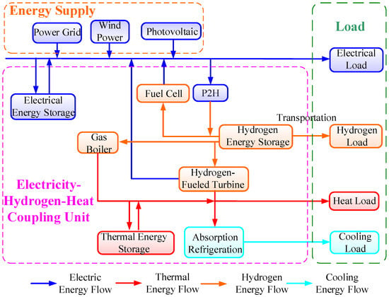
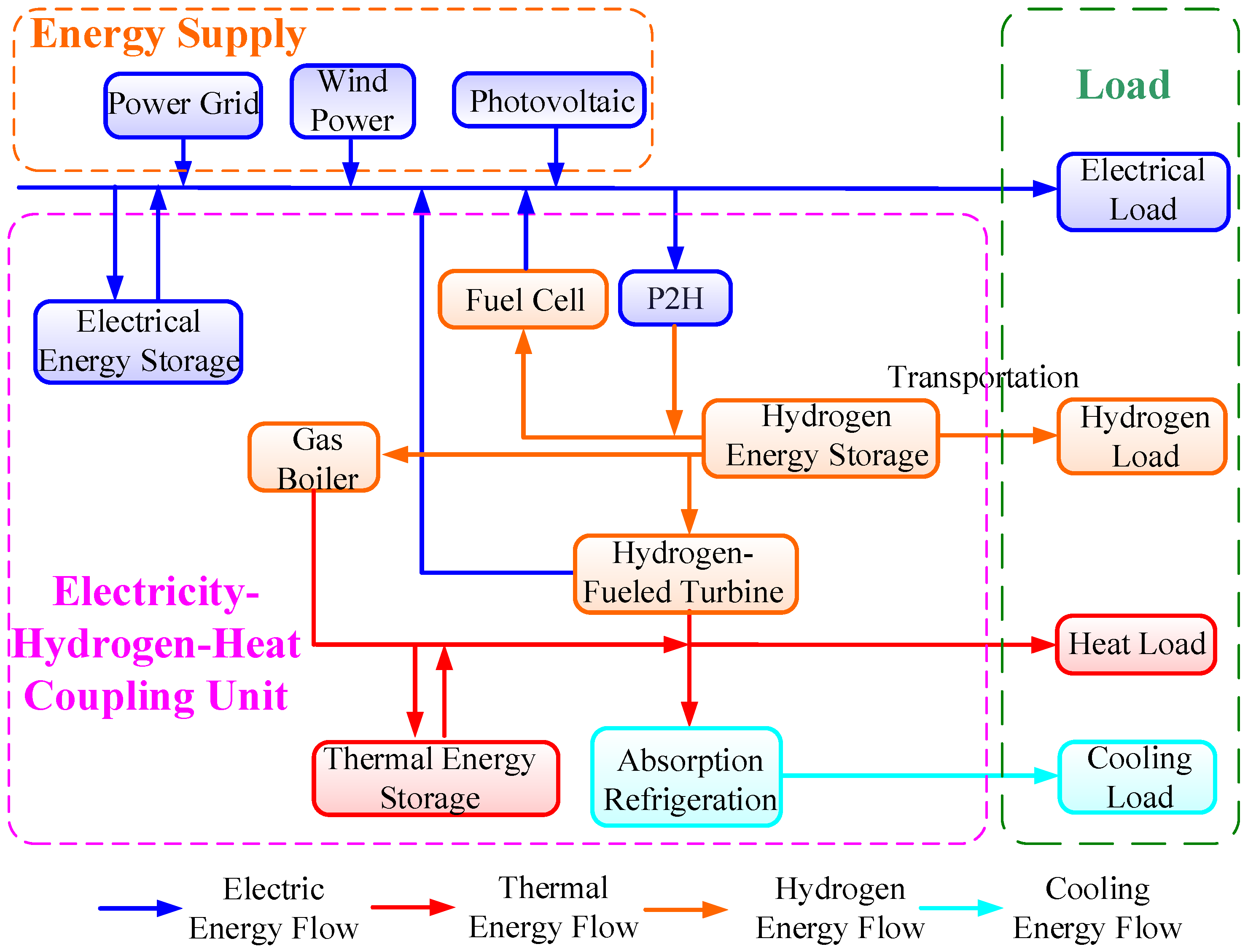
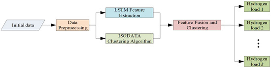
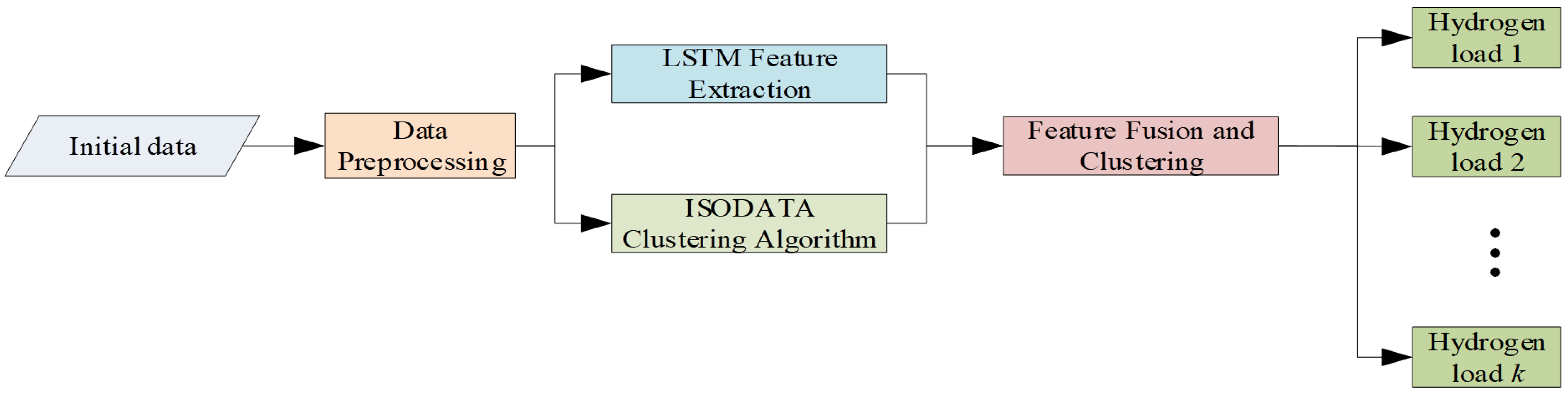
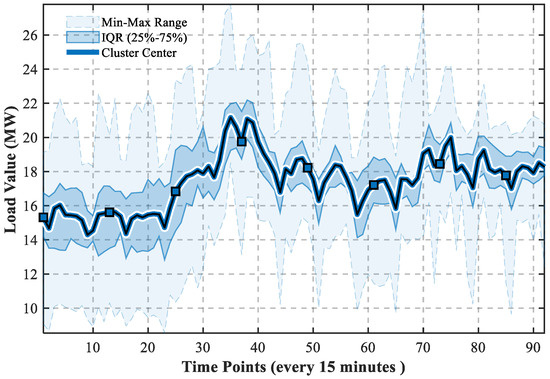
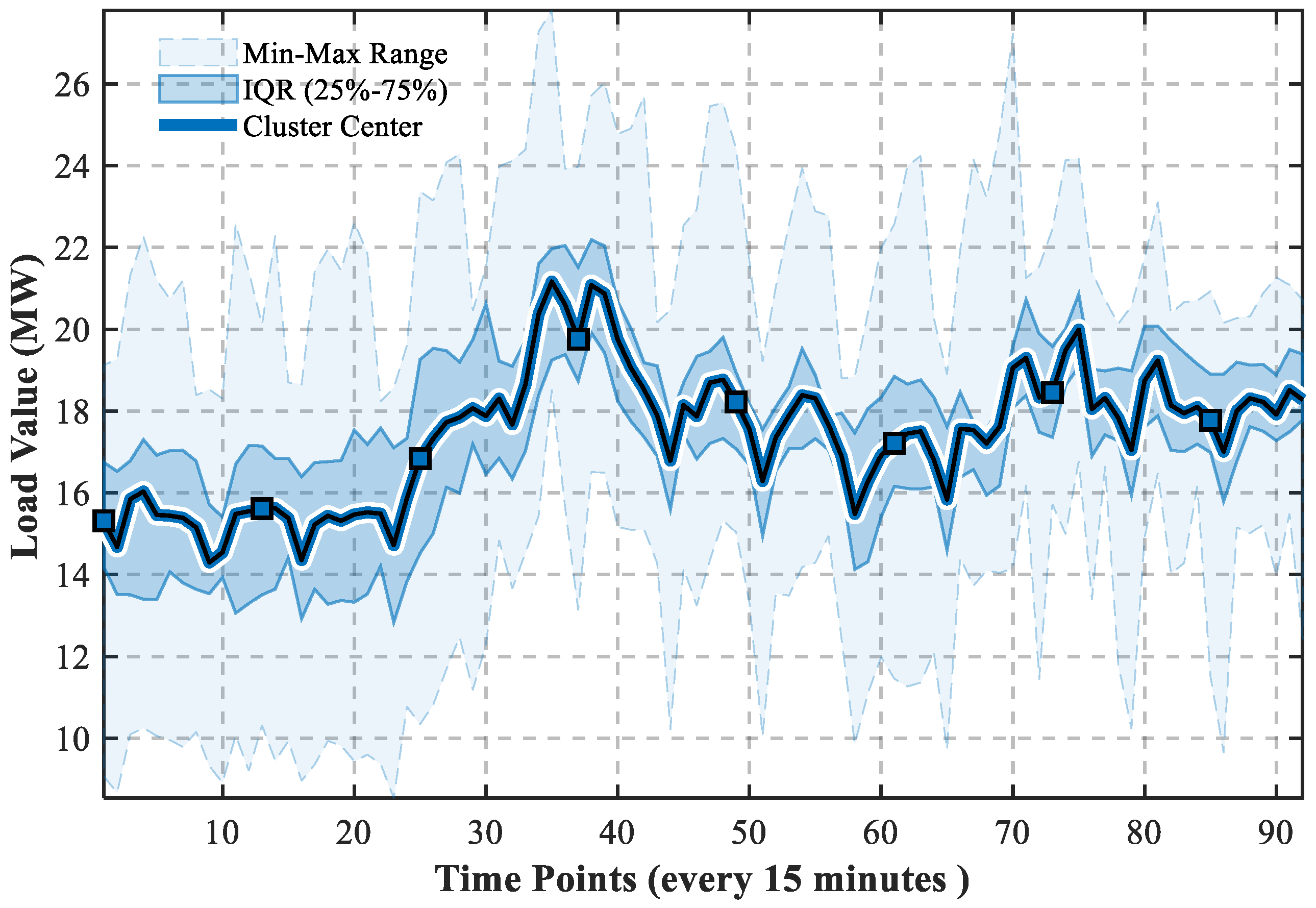
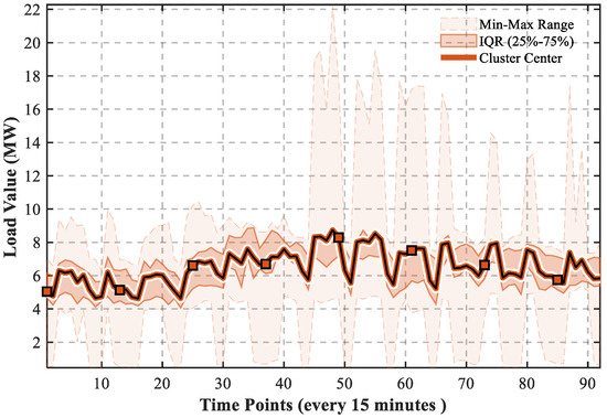
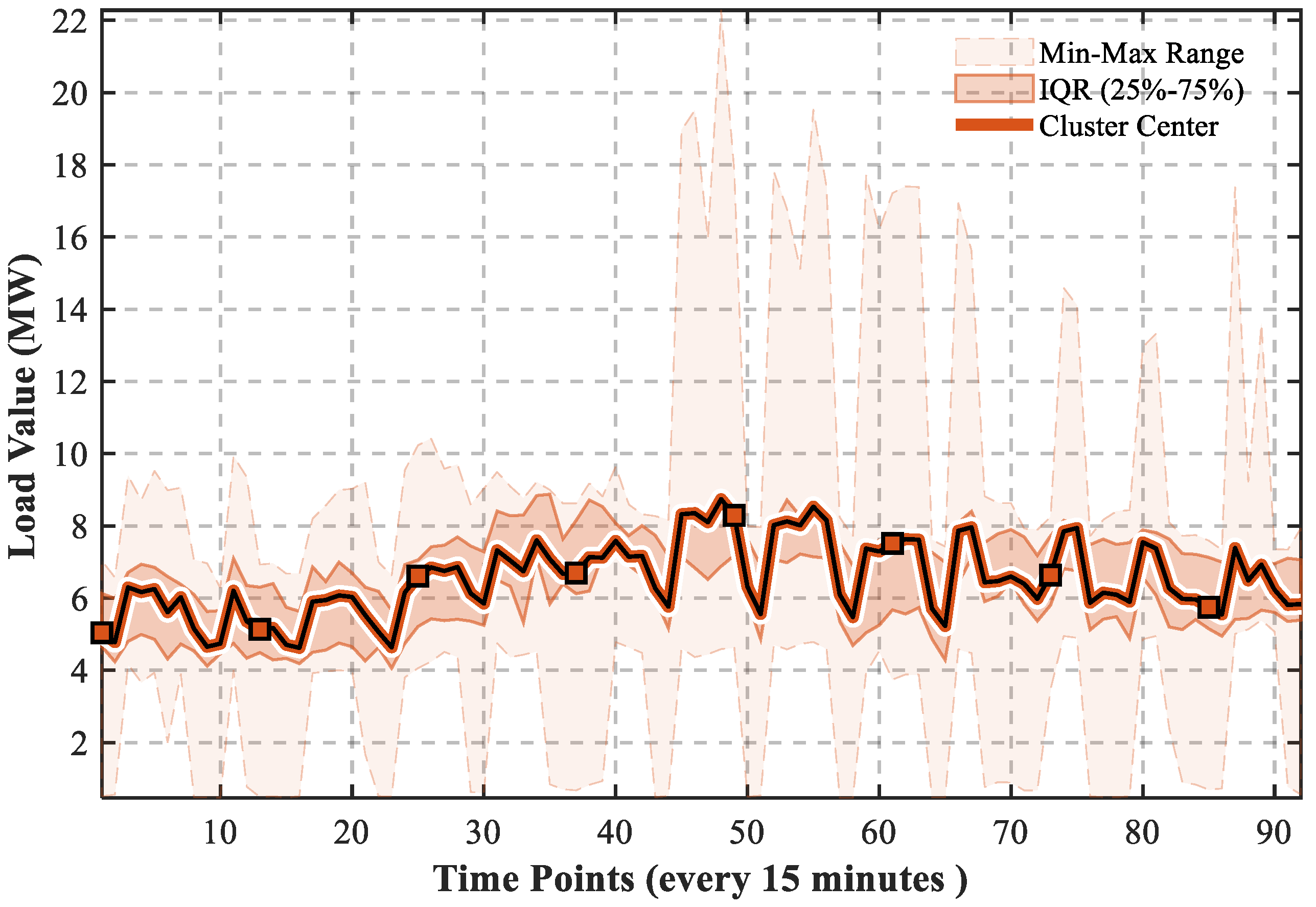
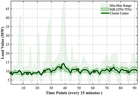
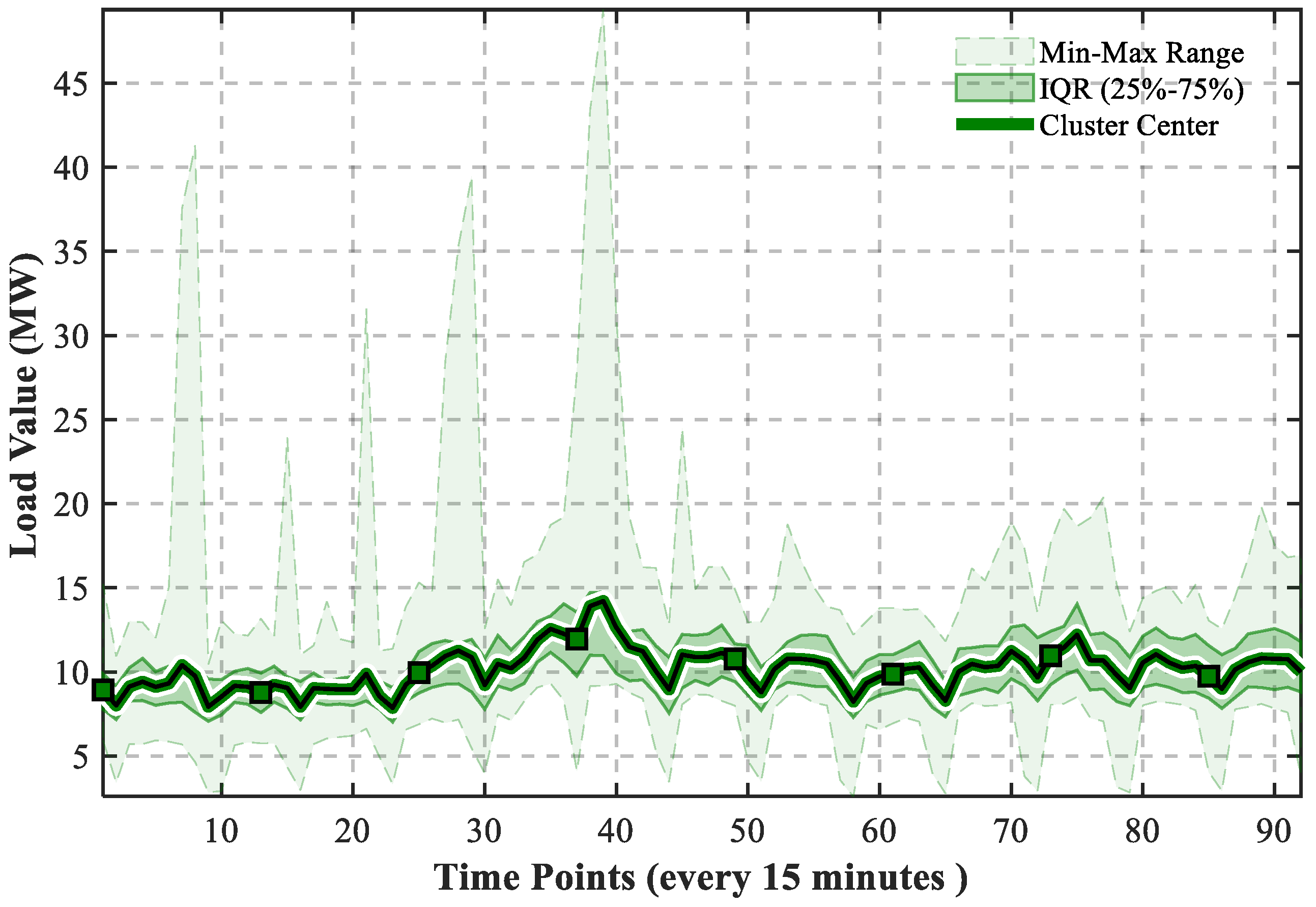
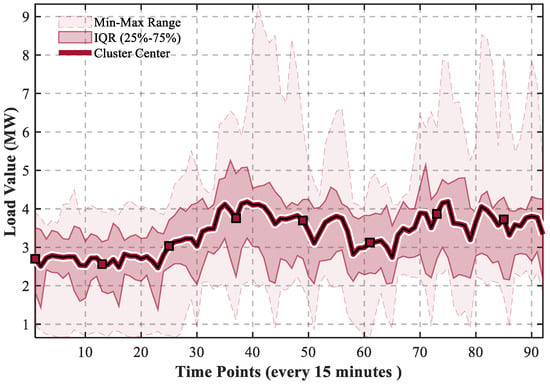
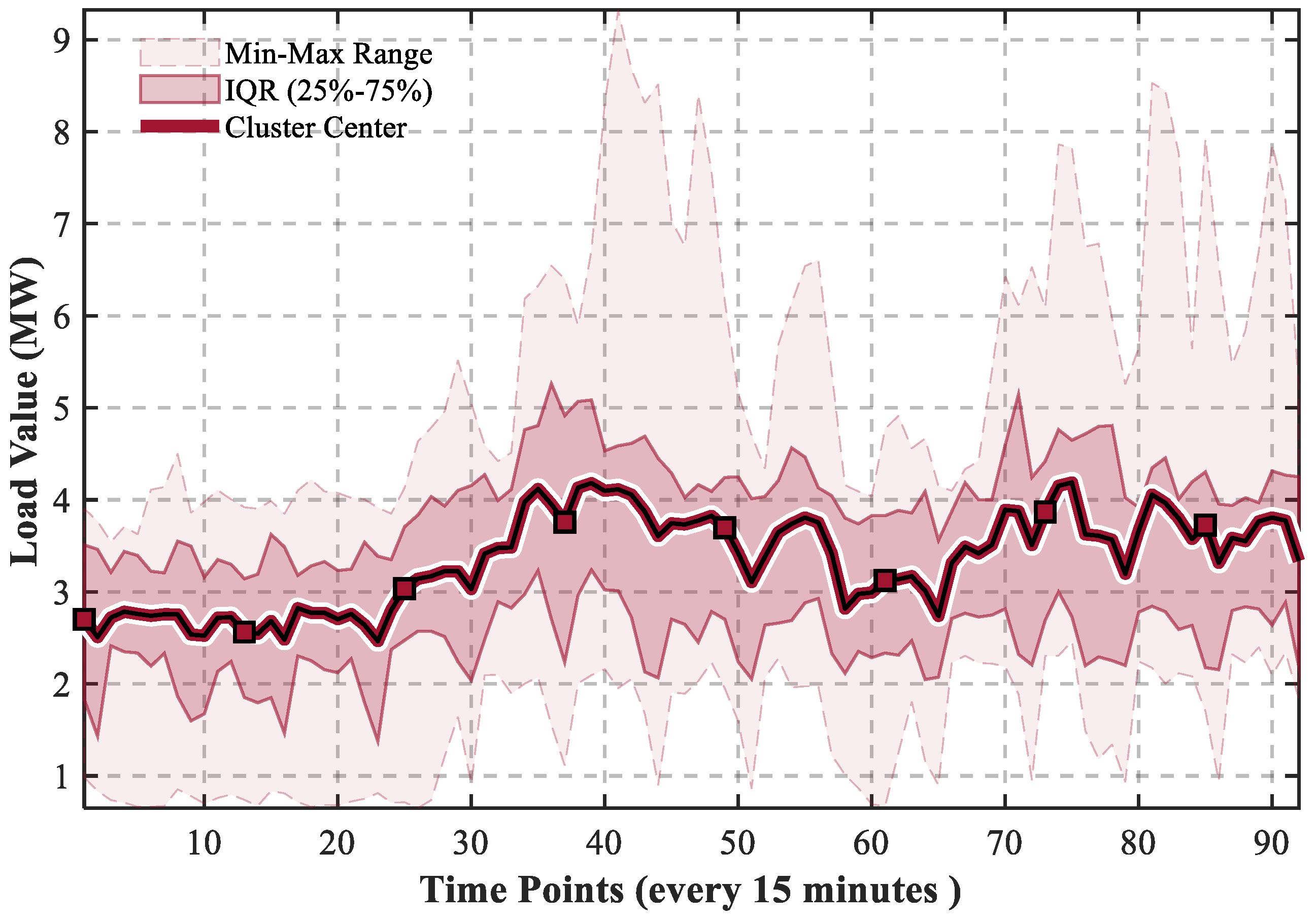
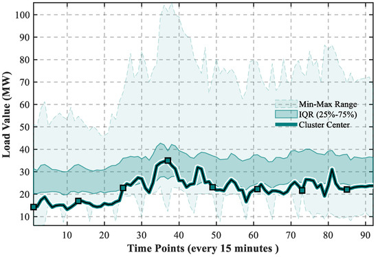
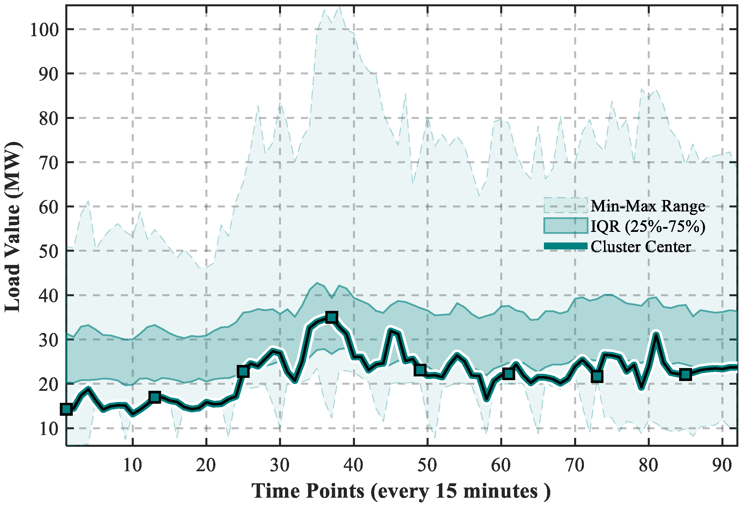
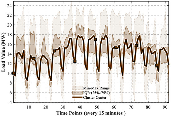
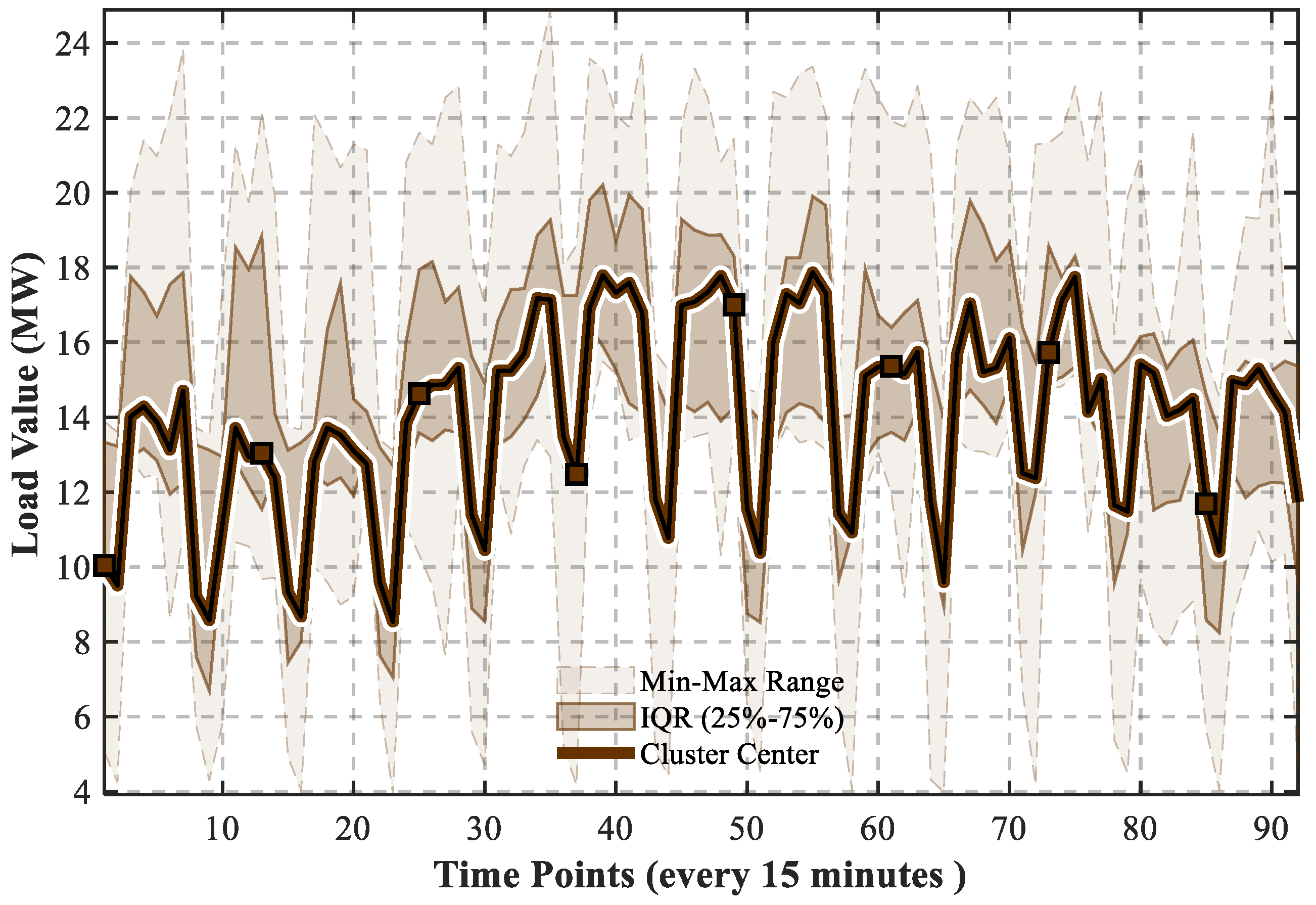
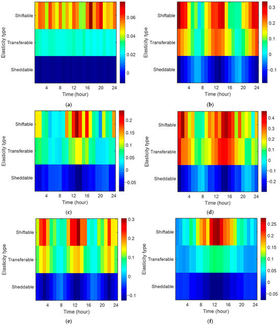
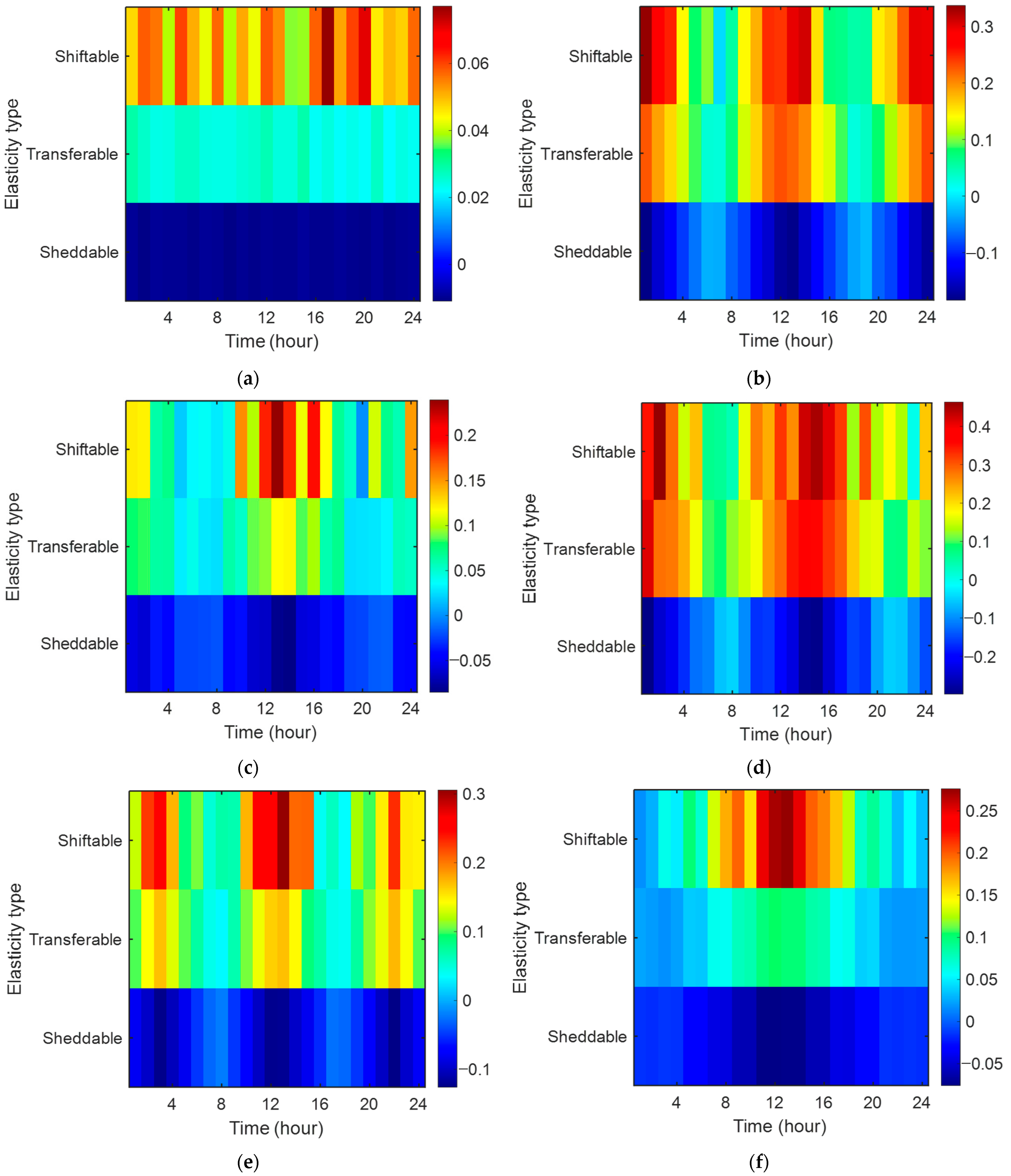
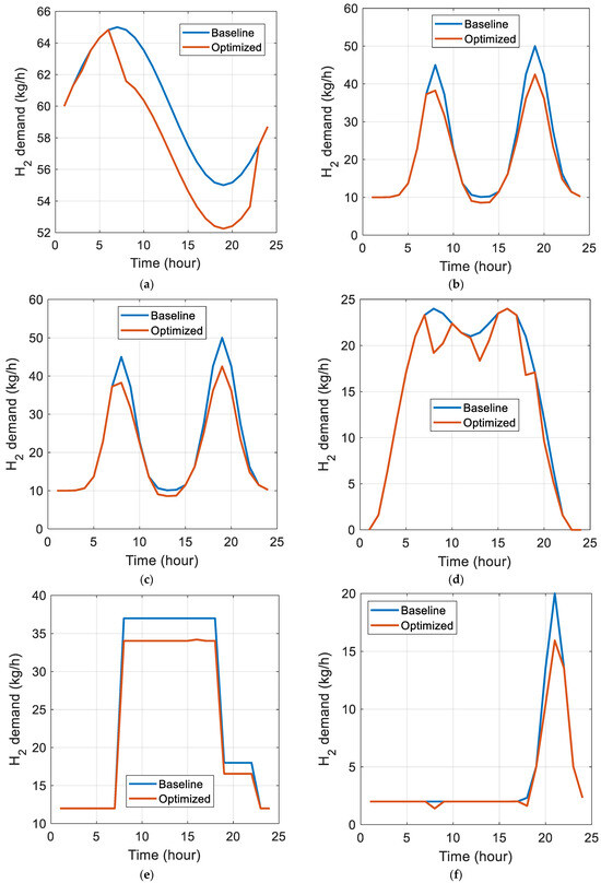
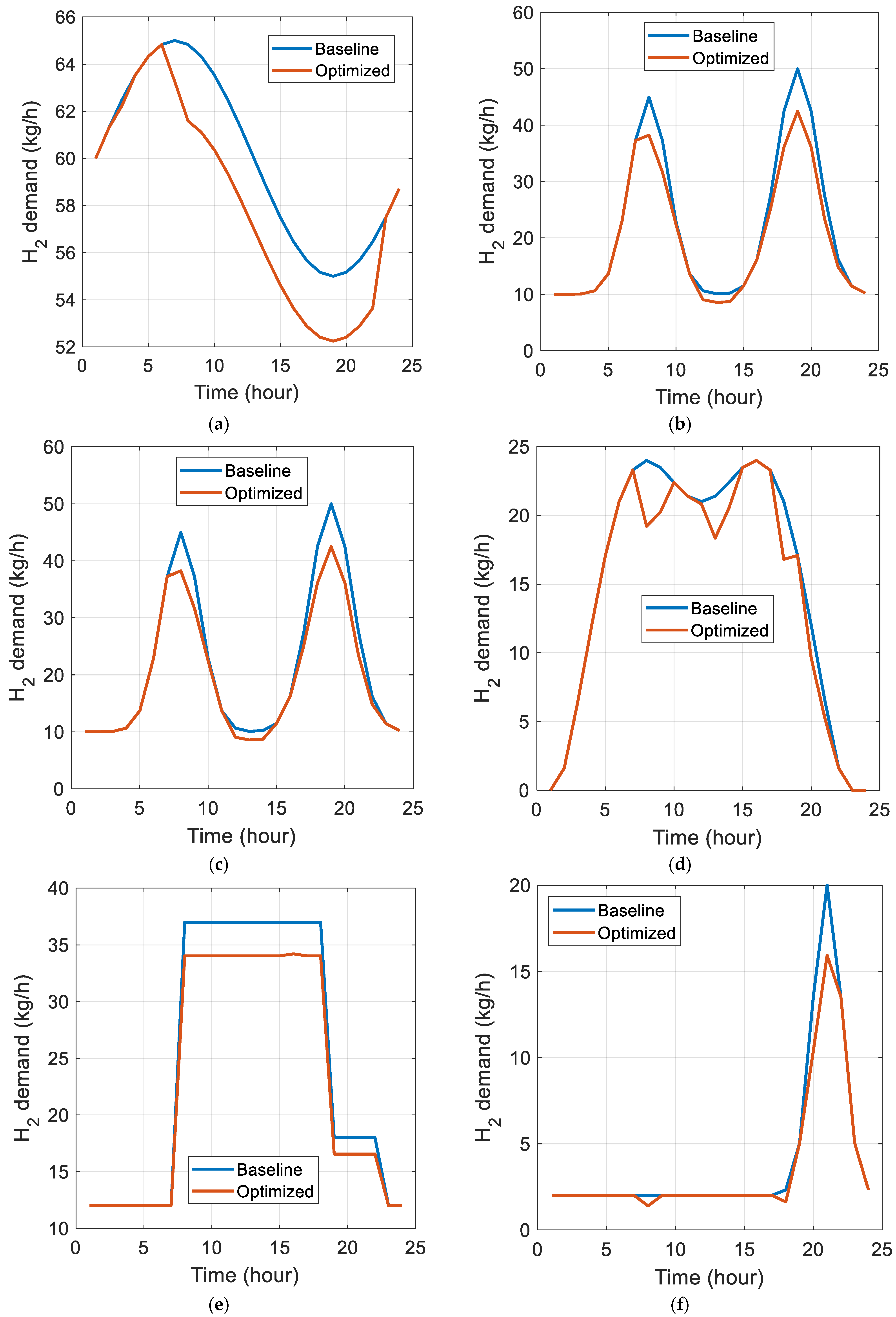
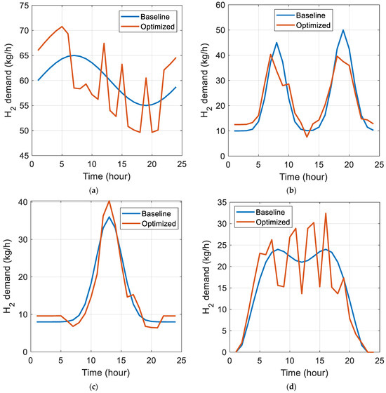
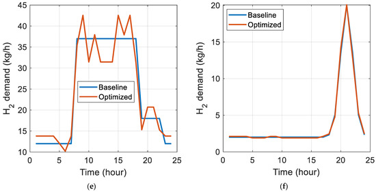
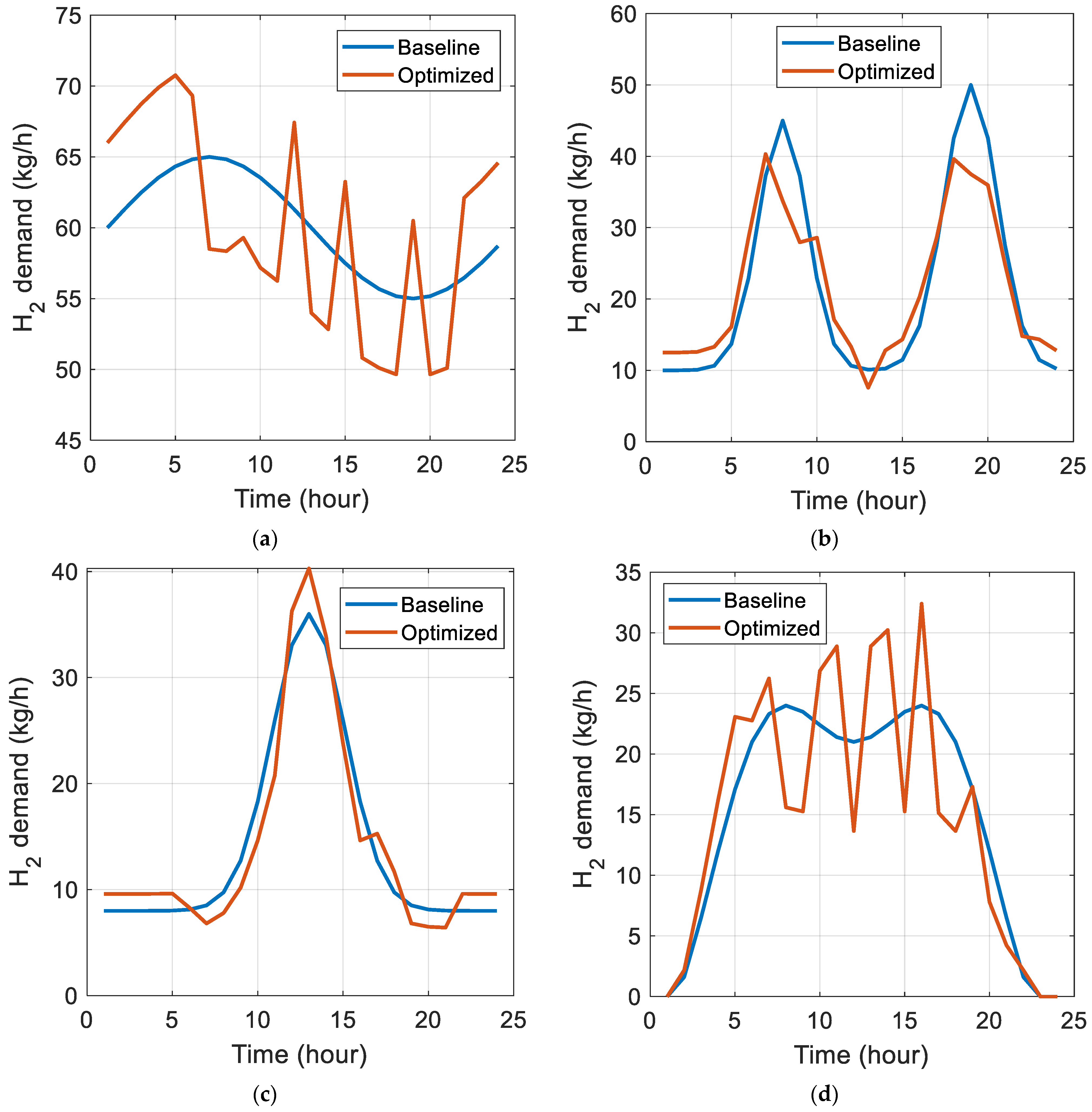
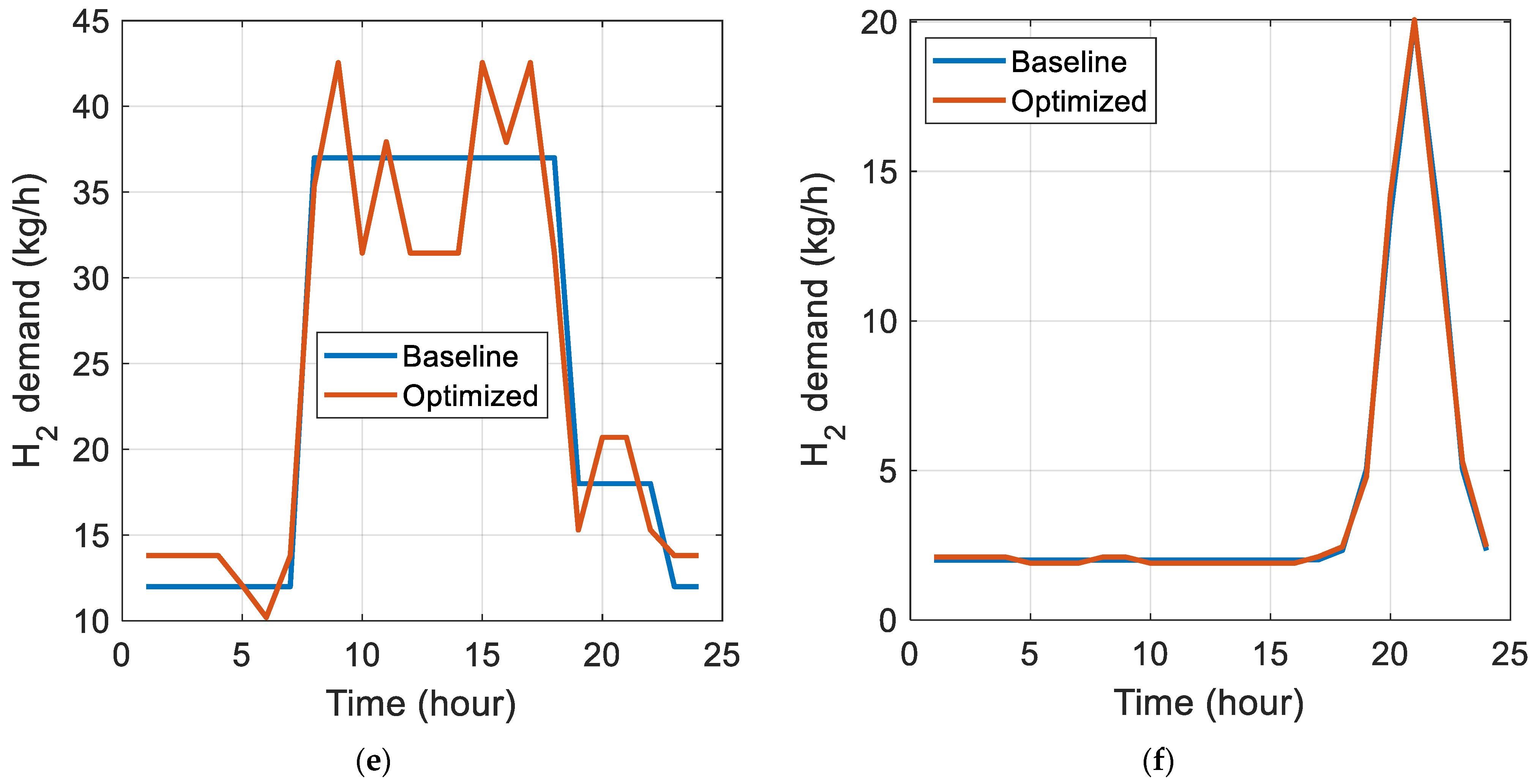
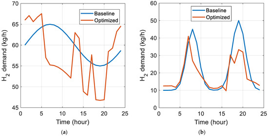
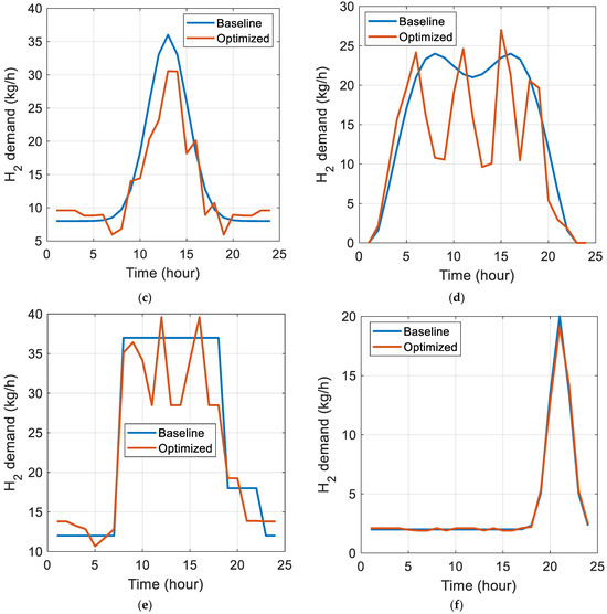
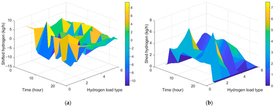
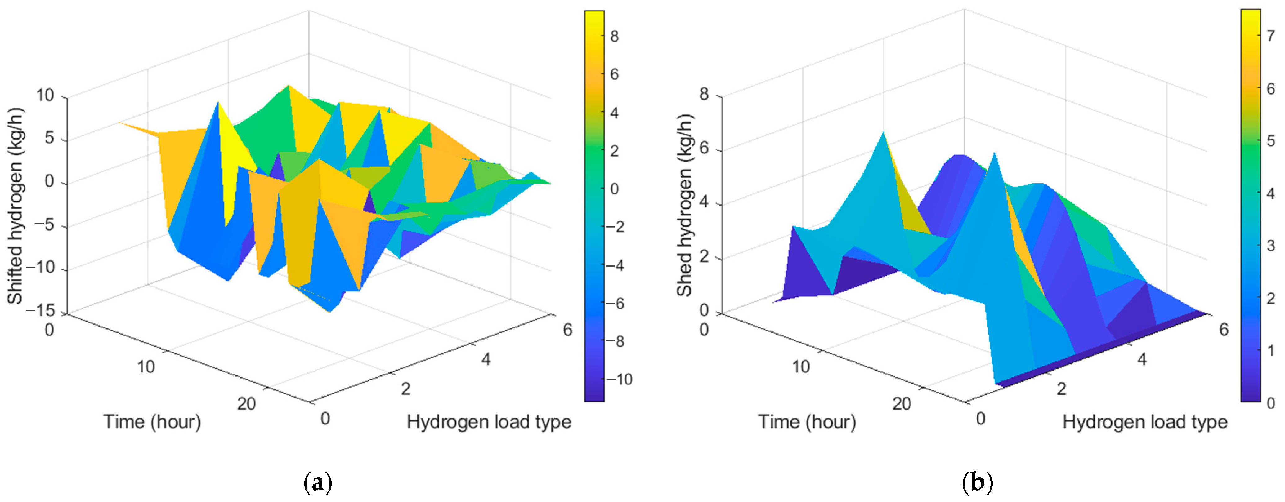
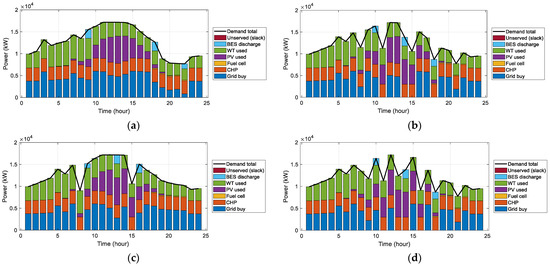
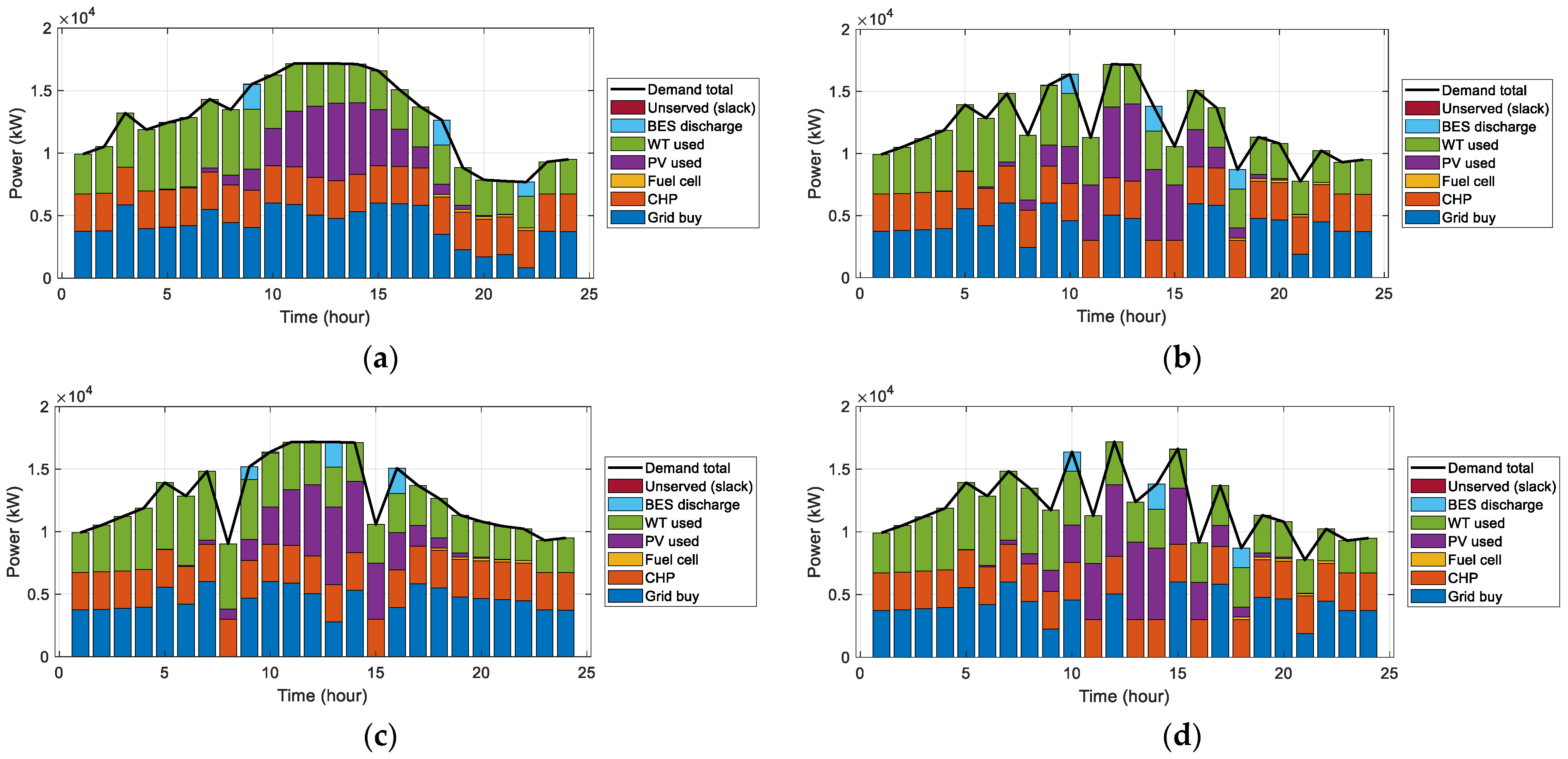

Disclaimer/Publisher’s Note: The statements, opinions and data contained in all publications are solely those of the individual author(s) and contributor(s) and not of MDPI and/or the editor(s). MDPI and/or the editor(s) disclaim responsibility for any injury to people or property resulting from any ideas, methods, instructions or products referred to in the content. |
© 2026 by the authors. Licensee MDPI, Basel, Switzerland. This article is an open access article distributed under the terms and conditions of the Creative Commons Attribution (CC BY) license.