Research on Power Grid Accident Analysis and Early Warning Model Based on Meteorological Factors

Abstract

Natural disasters and extreme meteorological events are primary causes of unplanned outages in modern power systems. Existing early warning methods suffer from insufficient non-linear feature extraction, severe class imbalance, and limited minority-class recall under single-classifier architectures. This paper proposes a seven-class meteorological fault early warning framework that integrates a sparse autoencoder (SAE), a G1–entropy composite weighting scheme, SMOTE oversampling, and a soft-voting BP–XGBoost ensemble. A leakage-free experimental protocol confines SMOTE exclusively to the training partition, eliminating data contamination from evaluation. Validated on 1955 fault records from a regional grid in East China covering 110 kV, 220 kV, and 500 kV voltage levels (2013–2022), the proposed framework achieved 96.42% accuracy and a 97.46% macro F1-score on the held-out test set, outperforming SVM (72.68%), Random Forest (89.31%), LSTM (81.47%), 1D-CNN (85.38%), and LightGBM (92.15%). Ablation experiments confirmed that SMOTE and G1–entropy weighting contributed macro F1 gains of 8.34 and 6.91 percentage points, respectively, while removing the XGBoost branch degraded accuracy by 28.25%. Temporal validation on 2019–2022 records yielded 91.57% accuracy, confirming temporal generalization. Error analysis further revealed that bidirectional misclassification between lightning damage and wind damage, rooted in shared atmospheric instability signatures, constitutes the dominant residual error source, providing theoretical guidance for future threshold optimization strategies.

1. Introduction

The wide-area coverage of power infrastructure and the continuous expansion of transmission lines have significantly increased the probability that new-type power systems are exposed to complex natural environments. A large number of distributed renewable energy generation units and flexible transmission equipment are deployed in these systems [1]. Due to their outdoor deployment characteristics, these components are highly sensitive to meteorological disturbances. Consequently, the risk of faults induced by natural disasters has become increasingly prominent [2,3].

Power grid operational faults are closely related to meteorological conditions. Such faults often exhibit wide impact ranges, severe economic losses, and strong chain reactions. These characteristics are particularly pronounced in the new-type power system architecture, where renewable energy serves as the primary power source. In this context, the volatility of weather and climate directly translates into uncertainty in grid operation, posing severe challenges to system security and stability [4,5,6].

China operates one of the largest power grids in the world, spanning diverse and complex geographical and climatic environments. This grid faces long-term threats from extreme weather events. Modern power systems rely heavily on power electronic equipment, whose reliability is severely challenged in extreme meteorological conditions, leading to a sharp increase in equipment failure risk [7,8]. For example, extreme events such as line icing and severe storms can easily cause physical damage. In systems with a high proportion of power electronics, such local faults can readily trigger widespread cascading disconnection accidents, seriously threatening power supply security and quality [9,10]. Therefore, to construct a new-type power system with high resilience it is essential to establish a proactive disaster prevention system with “source-grid-load-storage” coordination. The core of this system lies in achieving accurate perception of meteorological disaster-causing factors and providing advanced fault early warning.

Meteorological disasters are diverse in type and vary significantly in spatial and temporal distribution. They are often accompanied by secondary and derivative disasters, exhibiting obvious randomness and persistence. Renewable energy stations, such as wind farms and photovoltaic plants, are widely dispersed and highly dependent on environmental conditions. These characteristics make them more susceptible to concentrated impacts from regional extreme climates [11,12]. Such impacts not only cause physical damage to infrastructure but also severely degrade the prediction accuracy of renewable energy output. This degradation disrupts system power balance and consequently triggers power grid operational risks [13]. Historical lessons are instructive. The severe ice disaster in Southern China in 2008 caused devastating damage to traditional power grids. In the context of current new-type power systems, the scale of generator disconnection and the risk of system collapse would be exponentially amplified [14,15]. International cases also indicate that extreme weather is a major trigger of large-scale blackouts, while simultaneously highlighting the necessity of enhancing system resilience through measures such as energy storage and demand response [16,17].

To address the above challenges, extensive research has been conducted on early warning of meteorological disasters in power grids. Existing work has mostly focused on single disaster types. Representative studies include early warning of wildfire spread based on GIS and meteorological forecasts [18], lightning risk classification integrating multi-source monitoring [19], dynamic early warning of line icing considering micro-topography and meteorological elements [20], identification of vulnerable grid areas based on typhoon paths and wind monitoring data [21,22], prediction of insulator pollution levels [12], and self-powered temperature monitoring for substation contact early warning [23]. Furthermore, integrating multiple meteorological parameters to build comprehensive risk assessment models has become an important research direction [24]. For example, some studies have employed fuzzy membership functions and comprehensive indicators to quantify the relationship between meteorological factors and risk levels, thereby achieving dynamic risk assessment of transmission lines and power system oscillation early warning [25,26].

Although existing research has integrated meteorological data with power grid information platforms (e.g., GIS) to construct several early warning system frameworks and has introduced machine learning and deep learning methods—such as Support Vector Machines, convolutional neural networks, and ensemble architectures—to improve model performance [27,28,29], challenges remain. On one hand, given the massive, multi-dimensional, and heterogeneous nature of meteorological and grid data, the depth and efficiency of feature extraction are insufficient. On the other hand, under practical conditions such as sample imbalance and noise interference, the early warning sensitivity, generalization ability, and real-time performance of models still require improvement. These limitations lead to potential early warning delays or false alarms in practical applications, making it difficult to fully meet the urgent need for rapid and accurate fault early warning in new-type power systems [30].

The existing approaches suffer from three specific and interrelated deficiencies. In terms of feature representation, most prior models apply standard PCA or shallow neural networks that fail to capture non-linear coupling between meteorological variables, resulting in insufficient discrimination among physically similar disaster types such as lightning damage and wind damage. Regarding class imbalance, lightning damage typically accounts for more than 85% of historical events, and models trained without oversampling strategies consistently achieve minority-class recall below 60%, making them unreliable for rare but operationally critical scenarios. On the question of ensemble design, single-classifier architectures cannot simultaneously provide high accuracy for the majority class and dependable early warning for rare events, as the two objectives impose conflicting constraints on the decision boundary.

To address these gaps, this paper makes the following contributions. From a methodological perspective, a sparse autoencoder is employed for non-linear dimensionality reduction of 34-dimensional meteorological features, and a G1–entropy composite weighting scheme scientifically initializes feature importance prior to encoding. From an algorithmic perspective, SMOTE oversampling is applied exclusively to the training partition after stratified splitting, eliminating data leakage, and a soft-voting ensemble of BP and XGBoost achieves complementary generalization by leveraging the distinct strengths of gradient-based and tree-based classifiers. From an application perspective, a complete seven-class meteorological disaster warning framework is validated on a regional Chinese power grid dataset (110 kV, 220 kV, and 500 kV) spanning 2013–2022, achieving 96.42% accuracy and a 97.46% macro F1-score on the held-out test set.

2. Meteorological Disaster-Causing Feature Extraction Model Based on Sparse Autoencoder

2.1. Autoencoder

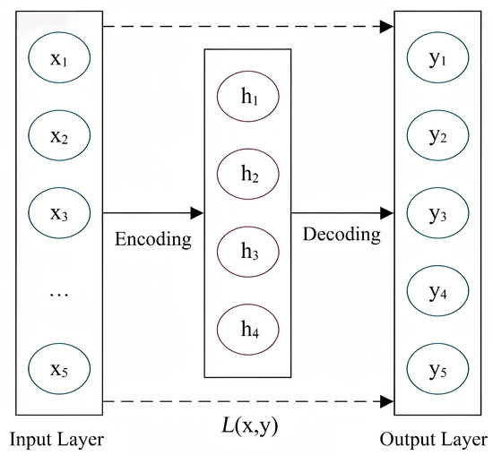
An autoencoder is a neural network with a symmetrical encoder–decoder architecture that learns compact data representations through unsupervised training. Its structure comprises three functional components: an input layer, a hidden layer, and an output layer. The encoder maps the high-dimensional input into a low-dimensional latent code, while the decoder reconstructs the original signal from this compressed representation. Network parameters are updated by minimizing the reconstruction error, which forces the hidden layer to retain only the most informative features of the data. As illustrated in Figure 1, this mirrored topology efficiently identifies key attributes of the input and provides a compact feature representation suitable for subsequent processing.

Figure 1. Architecture of autoencoder.

The task execution of an autoencoder is divided into two main stages: the encoding stage and the decoding stage. In the feature encoding stage, the Encoder network transforms the input data into latent features as shown in Equation  (1):

$$h=\sigma (Wx+b)$$

(1)

where h corresponds to the vector/scalar generated by the output layer, consistent with the row dimension of W; the sigmoid function is adopted as the activation function; the input feature vector x serves as the model input, typically with a dimension specification of $d\times 1$, where d is defined as the feature dimension size; and the weight matrix W and bias vector b constitute the connection parameters from the input layer (original data) to the hidden layer (feature data).

In the signal reconstruction stage, the output data is generated by the Decoder network through reconstruction from the latent features, as detailed in Equation (2):

$$y=\sigma (W^{\prime }h+b^{\prime })$$

(2)

where $W^{\prime }$ and $b^{\prime }$ represent the weight matrix and bias term from the hidden layer to the output layer (reconstructed data). The network adopts the sigmoid function $\sigma$ as the activation function, and the mathematical expression of this function along with its derivative characteristics is detailed in Equations (3) and (4):

$$\sigma \left(z\right)={\displaystyle \frac{1}{1+e^{-z}}}$$

(3)

$${\sigma }^{\prime }\left(z\right)=\sigma \left(z\right)(1-\sigma \left(z\right))$$

(4)

where in the sigmoid function, z represents the weighted input sum of the neuron. This activation function non-linearly compresses the input value into the interval $(0,1)$, and its output $\sigma \left(z\right)$ can be interpreted as a probability distribution or the activation intensity of the neuron. The first derivative ${\sigma }^{\prime }\left(z\right)$ of the function characterizes the sensitivity of the output value to changes in the input, reflecting the gradient variation characteristics of the activation state.

The core design objective of an autoencoder is to achieve high-precision reconstruction of the input data from the output data through an encoding–decoding mechanism. From a theoretical perspective, under ideal conditions, the network output should be able to completely reproduce the original input. The model quantifies the degree of difference between the input and output by defining a reconstruction error function $L(x,y)$, where the commonly used error function is composed of a combination of squared error and cross-entropy loss function. It is worth noting that when the encoding layer adopts the sigmoid activation function, the cross-entropy loss function becomes a more suitable error measurement method due to its mathematical properties, primarily because this function has a favorable synergistic effect with the sigmoid activation in terms of gradient computation.

The cross-entropy loss function is defined as:

$$L(x,y)=-{\displaystyle \sum _{i=1}^n}\left[x_{i}ln{y}_i+(1-x_i)ln(1-y_i)\right]+{\displaystyle \frac{\lambda }{2}}{\displaystyle \sum _{l=1}^{n_1}}\sum _i\sum _j{\left(W_{ij}^{\left(l\right)}\right)}^2$$

(5)

where $\lambda$ denotes the weight decay, which is used to control the model complexity; the network architecture contains $n_1$ hidden layers, where the number of neurons in the l-th layer is determined by $s\left(l\right)$; and the connection weights between layers are represented by matrices, with $W_{ij}^{\left(l\right)}$ specifically referring to the connection weight between the i-th neuron and the j-th neuron in the l-th layer.

For a neuron based on the sigmoid activation function, the value approaches 1 or approaches 0, reflecting the “activated state” and “resting state” of the neuron, respectively. To introduce sparsity constraints, the approach of constraining the number of activated neurons in the hidden layer is adopted, limiting the range of active neuron counts so that the features extracted by the network are both sparse and efficient.

The sparse autoencoder adjusts the activation degree of hidden layer neurons by means of a sparsity penalty term to achieve sparse activation. The sparsity constraint is generally defined as follows: measure the average activation level of hidden layer neurons, namely:

$${\widehat{\rho }}_j={\displaystyle \frac{1}{n}}{\displaystyle \sum _{i=1}^n}{a}_j\left(x^{\left(i\right)}\right)$$

(6)

where the neuron activation statistic ${\widehat{\rho }}_j$ represents the average activation level of the j-th neuron over the entire training set; n denotes the training batch size, i.e., the number of samples used for each parameter update; and the activation function output $a_j\left(x^{\left(i\right)}\right)$ is the response intensity of the j-th neuron when the i-th training sample $x^{\left(i\right)}$ is input.

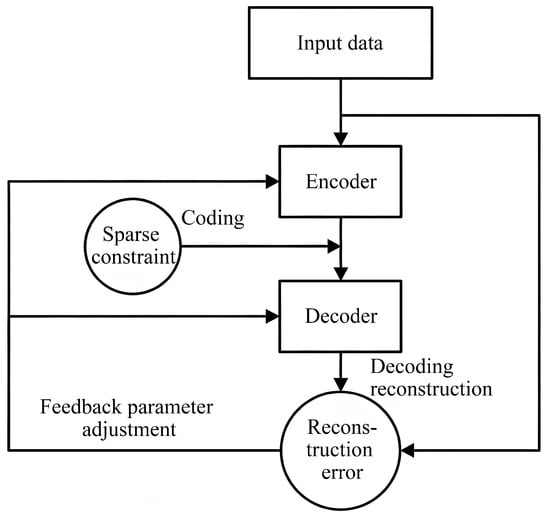
To achieve encoding sparsity, the Kullback–Leibler (KL) divergence is generally used to implement the sparsity penalty, constraining the firing level of hidden layer neurons. The abstract model of the sparse autoencoder is shown in Figure 2.

Figure 2. Abstract model of sparse autoencoder.

Combining the reconstruction error and the sparsity penalty term, the loss function under sparsity constraints is proposed as follows:

$$L_{\mathrm{sparse}}=L(x,y)+\beta {\displaystyle \sum _{j=1}^{s_2}}\mathrm{KL}(\rho \Vert {\widehat{\rho }}_j)$$

(7)

where $\beta$ is the control weight of the sparsity factor and $\theta$ is the random number used in the process of parameter initialization of the network. After setting the objective function, a layer-wise greedy algorithm is used to iteratively compute the objective function to minimize the loss function:

$$W_{ij}^{\left(l\right)}=W_{ij}^{\left(l\right)}-\alpha {\displaystyle \frac{\partial L_{\mathrm{sparse}}}{\partial W_{ij}^{\left(l\right)}}}$$

(8)

$$b_i^{\left(l\right)}=b_i^{\left(l\right)}-\alpha {\displaystyle \frac{\partial L_{\mathrm{sparse}}}{\partial b_i^{\left(l\right)}}}$$

(9)

where $\alpha$ denotes the learning rate parameter, which controls the step size magnitude of the weight updates. When the objective function value converges to a preset threshold, the optimization process of the encoding stage terminates.

2.2. Stacked Autoencoder

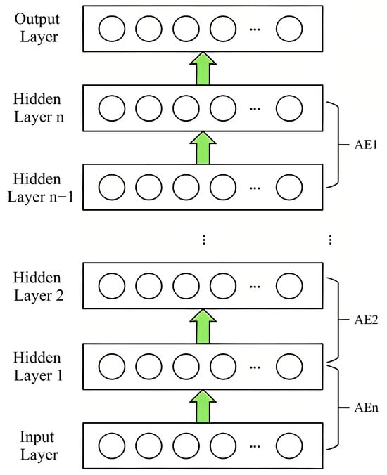
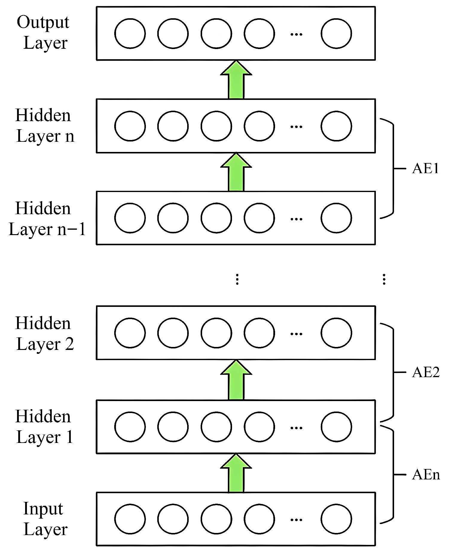
A stacked sparse autoencoder (SAE) is formed by composing multiple autoencoder layers in depth, endowing the model with the capacity to learn increasingly abstract and discriminative feature representations. Each constituent encoder reduces the dimensionality of its input and produces a compact latent code, while the paired decoder reconstructs the original signal; training minimizes the reconstruction discrepancy, driving the encoder to retain progressively more informative abstractions. The resulting multi-layer architecture, illustrated in Figure 3, achieves hierarchical feature learning that surpasses what a single shallow autoencoder can provide.

Figure 3. Network architecture of stacked autoencoder.

3. XGBoost-Based Fault Early Warning Model for Meteorological Disasters in Power Grids

Starting from the theories of ensemble learning and gradient boosting, XGBoost (eXtreme Gradient Boosting) achieves machine learning modeling by constructing a series of sequentially generated decision trees. The model is based on gradient descent optimization in function space and regularized structural risk minimization theory, aiming to efficiently process high-dimensional, non-linear data and accomplish accurate classification and regression tasks. Its core lies in iteratively optimizing the objective function in an additive manner, reducing bias while effectively controlling model complexity, thereby achieving excellent generalization performance even under conditions of limited samples or noisy data.

The training process of XGBoost aims to minimize an objective function $L^{\left(t\right)}$ that consists of a loss function and a regularization term. This function is defined in the t-th round of iteration as follows:

$$L^{\left(t\right)}={\displaystyle \sum _{i=1}^n}l\left(y_i,{\widehat{y}}_i^{(t-1)}+f_t\left(x_i\right)\right)+\Omega \left(f_t\right)$$

(10)

where n is the total number of samples; $y_i$ is the true label (fault type) of the i-th sample; ${\widehat{y}}_i^{(t-1)}$ is the ensemble prediction value of the first $(t-1)$ trees; $f_t\left(x_i\right)$ is the prediction output of the t-th tree to be constructed; $l(·)$ is a differentiable loss function (e.g., logarithmic loss function for classification), which measures the difference between the predicted value and the true value; and $\Omega \left(f_t\right)$ is the regularization term that controls the complexity of the t-th tree.

The specific expression of the regularization term $\Omega \left(f\right)$ is

$$\Omega \left(f\right)=\gamma T+{\displaystyle \frac{1}{2}}\lambda {\displaystyle \sum _{j=1}^T}{w}_j^2,$$

(11)

where T represents the total number of leaf nodes in the decision tree; $w_j$ denotes the score (weight) of the j-th leaf node; $\gamma$ is the complexity penalty parameter controlling leaf node splitting, where a larger value results in a simpler model structure; and $\lambda$ is the L2 regularization weight parameter, which prevents the leaf node weights from becoming too large, thereby effectively suppressing model overfitting.

To solve efficiently, XGBoost performs a second-order Taylor expansion of the objective function $L^{\left(t\right)}$ and removes the constant terms. By defining the first derivative $(g_i={\partial }_{{\widehat{y}}^{(t-1)}}l(y_i,{\widehat{y}}^{(t-1)}))$ and the second derivative $(h_i={\partial }_{{\widehat{y}}^{(t-1)}}^{2}l(y_i,{\widehat{y}}^{(t-1)}))$ for each sample, the approximate optimization problem of the objective function can be transformed into finding the optimal tree structure. For a tree with a fixed structure q (which maps samples to leaf nodes), the optimal leaf node weight $w_j^{\ast }$ and the corresponding minimum objective function value $L^{\left(t\right)\ast }$ can be obtained analytically as follows:

$$w_j^{\ast }=-{\displaystyle \frac{{\sum }_{i\in I_j}{g}_i}{{\sum }_{i\in I_j}{h}_i+\lambda }}$$

(12)

$$L^{\left(t\right)\ast }=-{\displaystyle \frac{1}{2}}{\displaystyle \sum _{j=1}^T}{\displaystyle \frac{{\left({\sum }_{i\in I_j}{g}_i\right)}^2}{{\sum }_{i\in I_j}{h}_i+\lambda }}+\gamma T$$

(13)

where $I_j$ represents the set of all samples assigned to the j-th leaf node. Equation (13) is used as a scoring function (also referred to as “gain”) to evaluate the splitting benefit of candidate tree structures. During the tree growth process, the algorithm selects the feature and split point that maximize this gain.

After M rounds of iteration, the final XGBoost ensemble model consists of M decision trees. For a new input meteorological feature vector x, the final fault category prediction (or fault probability) is obtained by summing the outputs of all the trees. The decision function can be expressed as

$$\widehat{y}\left(x\right)={\displaystyle \sum _{t=1}^M}{f}_t\left(x\right),$$

(14)

where $\widehat{y}\left(x\right)$ is the final output of the model for the input x and $f_t\left(x\right)$ is the prediction score of the t-th decision tree for x.

In this study, the deep meteorological disaster-causing feature vectors extracted by the SAE are used as the input x to the XGBoost model. By optimizing the above process, the model learns the mapping relationship from the high-dimensional, complex feature space to the power grid fault category labels (e.g., lightning strike, icing, wind damage, etc.). By adjusting hyperparameters, such as the number of iteration rounds M, learning rate, maximum tree depth, $\gamma$, and $\lambda$, and by combining cross-validation with grid search strategies a high-precision and robust classification early warning model for power grid meteorological disaster-induced faults can be constructed. This model not only outputs accurate fault type predictions but also quantifies the importance of different meteorological factors in fault prediction by calculating the total split gain of each feature during the model construction process, thereby enhancing the interpretability of the early warning decision-making.

4. Modeling and Fault Prediction Method for Power Grid Meteorological Disaster Early Warning

4.1. Data Preprocessing

Due to the involvement of multiple meteorological parameters in the power grid meteorological fault warning model, significant differences in dimensions and magnitudes exist among these parameters. Directly inputting them into the model would affect the training effectiveness and convergence speed. Therefore, it is necessary to preprocess the raw meteorological data before feature extraction and model training.

The dimensions and units of various meteorological parameters differ, and their value ranges may vary significantly, with extreme differences reaching hundreds or even thousands of times. To reduce the computational complexity of the model, it is necessary to normalize the initial data of all factors and unify the dimensions of the data.

In this paper, range standardization is selected to normalize the data samples. The normalization formula is as follows:

$$x_i^{\ast }={\displaystyle \frac{x_i-min\left\{x\right\}}{max\left\{x\right\}-min\left\{x\right\}}}$$

(15)

where x is the original data sample of each type of meteorological factor; $x_i^{\ast }$ is the new input sample of that factor after normalization; $x_i$ and $x_i^{\ast }$ correspond to the i-th sample data in x and $x^{\ast }$ within the meteorological dataset, respectively; and $max\left\{x\right\}$ and $min\left\{x\right\}$ are the maximum and minimum values in the original data sample, respectively. The data processed by range standardization exhibits good numerical stability and can significantly improve the convergence and learning ability of the autoencoder.

The proposed framework for power grid meteorological disaster prevention integrates a sparse autoencoder (SAE) with SMOTE oversampling and an ensemble classifier. The SAE is distinct from a denoising autoencoder (which corrupts inputs) and from a contractive autoencoder (which penalizes the Jacobian norm); it imposes a KL-divergence sparsity penalty ($\rho =0.05$, $\beta =0.1$) on hidden activations to learn compact, discriminative feature representations from 34-dimensional meteorological inputs.

The experimental pipeline follows seven sequential steps to eliminate data leakage: (Step 1) Stratified 80/20 train–test split (random_state = 42) on the 1955-sample experimental dataset, yielding a training set of 1564 samples and a fixed test set of 391 samples; (Step 2) StandardScaler fitted on the training set only and identically applied to the test set; (Step 3) G1–entropy composite weights computed on training-set features only; (Step 4) SMOTE ($k=5$) applied exclusively to the training partition to oversample minority-class instances and mitigate class imbalance—the test set is never resampled; (Step 5) SAE ($34\to 24\to 18\to 14$) trained on the SMOTE-balanced training set; (Step 6) BP and XGBoost trained on SAE-encoded training features; (Step 7) evaluation on the held-out test set (391 samples).

Based on the SMOTE algorithm, sample enhancement of the training data is completed and the fault sample set is expanded. The SMOTE algorithm selects neighboring sample points of the minority class according to Euclidean distance and randomly creates new samples in the feature space using Equation (16) to achieve incremental expansion of fault class samples. The augmented samples maintain the class division of the original samples while not disturbing the distribution structure of the original samples, thereby maintaining the proportional balance between fault and normal samples. Critically, SMOTE is applied only to the training partition after the train–test split is completed, so no synthetic sample derived from test-set instances contaminates the training set. Using this method, the class imbalance of the initial samples is alleviated, and prediction errors caused by insufficient fault samples are effectively suppressed:

$$z_i=x+\mathrm{rand}(0,1)\times (y^{\left(i\right)}-x)$$

(16)

where x represents the starting vector (fixed); $y^{\left(i\right)}$ is the i-th endpoint vector (there may be multiple y samples); $\mathrm{rand}(0,1)$ is a random number uniformly distributed in the interval $[0,1]$; and $z_i$ is the interpolation result, a random point lying between x and $y^{\left(i\right)}$.

4.2. Composite Weighting of Disaster-Causing Factors Based on the G1–Entropy Method

The composite weighting procedure integrates two complementary perspectives on factor importance. The G1 method assigns subjective weights by ranking the disaster-causing factors in order of significance and converting expert judgments into numerical importance ratios, thereby producing a subjective weight for each factor. The entropy weight method then quantifies objective weights by measuring the degree of variability in each factor’s observed distribution: factors whose values exhibit greater dispersion carry more discriminative information and accordingly receive higher objective weights. Combining these two sets of weights through Lagrange-multiplier optimization yields composite weights that simultaneously reflect domain expertise and the statistical characteristics of the historical data, providing a scientifically rigorous basis for feature initialization in the subsequent learning stage.

4.2.1. G1 Subjective Weighting Method

The G1 subjective weighting was conducted by a panel of five senior power-grid meteorology engineers (all with more than ten years of field experience in power-system meteorological risk assessment). A three-round Delphi procedure was employed: each expert independently assigned importance ratios $r_k$ in Round 1; anonymized group results were fed back between rounds; a consensus ranking was reached in Round 3. Kendall’s concordance coefficient $W=0.81$ ($p<0.01$) confirmed high inter-expert agreement.

Let $x_1,x_2,\cdots ,x_n$ be n indicators in a multi-indicator system, which in this paper refer to the meteorological factors. First, the most important factor is selected and denoted as $x_1$. If the importance of $x_i$ is higher than that of $x_j$, it is denoted as $x_i\ge x_j$. When the meteorological factors satisfy the following relationship: $x_1\ge x_2\ge \cdots \ge x_n$, they are said to establish an order relationship. After determining the order relationship, quantitative analysis can be performed on each indicator. The analysis method is shown in Equation (17):

$${\omega }_k=r_k{\omega }_{k-1},k=n,n-1,\cdots ,2$$

(17)

where ${\omega }_k$ is the subjective weight of the k-th factor and $r_k$ represents the ratio of importance between $x_{k-1}$ and $x_k$. Based on the rational assignment of $r_k$ given by experts, ${\omega }_n$ is:

$${\omega }_n={\displaystyle \frac{1}{1+{\sum }_{k=2}^n{\prod }_{i=k}^n{r}_i}}$$

(18)

$${\omega }_{k-1}=r_k{\omega }_k$$

(19)

$${\displaystyle \sum _{k=1}^n}{\omega }_k=1$$

(20)

${\omega }_n$ is the calculation formula for the subjective weight of the factor determined based on expert decision-making. After calculating ${\omega }_n$, the subjective weights of the other factors are obtained according to the formula.

4.2.2. Entropy Weight Method

The entropy weight method calculates the degree of dispersion of indicators through information entropy. It is an important weighting approach in decision analysis and is particularly adept at solving complex evaluation problems. This method, which is based on entropy value calculation, analyzes the importance of each indicator and thereby obtains the weight allocation for each indicator. To conduct research using the entropy weight method, the initial evaluation matrix must first be established. Assuming the experimental sample size consists of m objects, a matrix R can be formed based on the sample objects with n evaluation indicators:

$$R={\left(r_{ij}\right)}_{m\times n}$$

(21)

where $r_{ij}$ represents the score of the j-th indicator for the i-th evaluation object.

The characteristic proportion $p_{ij}$ of $r_{ij}$ is calculated by Equation (22):

$$p_{ij}={\displaystyle \frac{r_{ij}}{{\sum }_{i=1}^m{r}_{ij}}}$$

(22)

where $r_{ij}$ corresponds to the element in the i-th row and j-th column of the original matrix or vector (non-negative real number); $p_{ij}$ is the normalized result; and m is the number of rows (or the dimension size to be normalized).

The information entropy $H_j$ and entropy weight ${\omega }_j$ of the j-th indicator can be obtained from Equations (23) and (24):

$$H_j=-{\displaystyle \frac{1}{lnm}}{\displaystyle \sum _{i=1}^m}{p}_{ij}ln{p}_{ij}$$

(23)

where $p_{ij}$ is the probability value of the i-th row and j-th column; m is the number of rows (or the number of possible states); $H_j$ is the entropy of the j-th column, which measures the uncertainty of the probability distribution of that column; and $lnm$ is the normalization factor that ensures $H_j\in [0,1]$ (the maximum entropy is 1).

$${\omega }_j={\displaystyle \frac{1-H_j}{{\sum }_{j=1}^n(1-H_j)}}$$

(24)

where $H_j$ represents the entropy (uncertainty) of the j-th column, with a value range of $[0,1]$ (calculated by the previous formula), and $1-H_j$ is the certainty of the j-th column (the complement of entropy). The smaller the entropy, the higher the certainty; ${\omega }_j$ is the weight of the j-th column.

When the numerical difference of the same factor is larger, it indicates that the factor can provide more effective information. Consequently, the entropy value of that factor becomes smaller and the weight becomes larger, and vice versa.

4.2.3. Combined Weighting Method

The combined subjective and objective weights are calculated by the Lagrange multiplier algorithm as follows:

$${\omega }_k={\displaystyle \frac{{\omega }_i{\omega }_j}{{\sum }_{k=1}^n{\omega }_i{\omega }_j}}$$

(25)

where ${\omega }_k$ is the combined weight of the disaster-causing factor obtained by combined weighting; ${\omega }_i$ is the subjective weight of the disaster-causing factor obtained by subjective weighting; and ${\omega }_j$ is the objective weight of the disaster-causing factor obtained by the entropy weight method.

The initial weight of each meteorological factor is determined by the combined weighting method. Subsequently, these initially weighted meteorological factors are input into the sparse autoencoder (SAE) for feature extraction. During the feature extraction process, the weights of the 34-dimensional meteorological factors are dynamically adjusted and optimized as the number of model iterations increases, thereby achieving adaptive learning of the importance of different meteorological factors.

4.3. Deep Feature Extraction Based on Sparse Autoencoder (SAE)

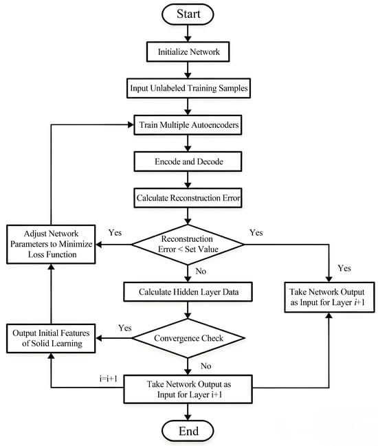
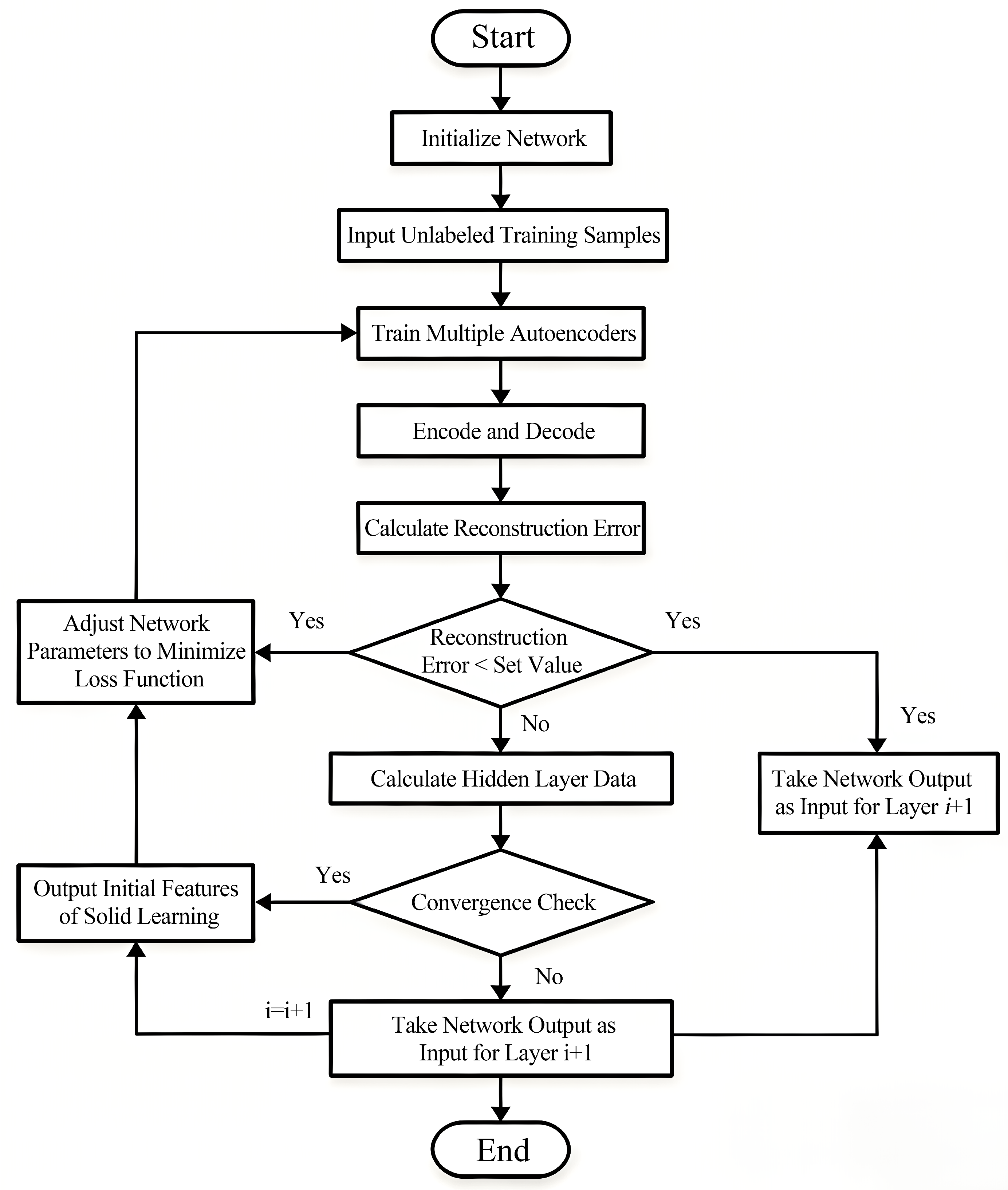
The model used in this study was a stacked SAE, which imposes a KL-divergence sparsity penalty on hidden-layer activations; it is distinct from a denoising autoencoder (which corrupts inputs) and from a contractive autoencoder (which penalizes the Jacobian norm). The feature extraction process of the SAE proceeds through two sequential stages. During the unsupervised pre-training stage, a layer-wise greedy strategy is adopted: each autoencoder layer is optimized independently, with its parameters initialized by minimizing the per-layer reconstruction loss. Upon convergence of a given encoder layer, its output representation is passed as the input to the subsequent layer, and this process continues until all encoder layers have been trained, yielding a preliminary deep feature set of the disaster-causing factors. The workflow of this unsupervised pre-training stage is illustrated in Figure 4.

Figure 4. Fundamental workflow of unsupervised pre-training.

After the entire pre-training process of the stacked autoencoder is completed, the output results of the deep hidden layers are redefined as a feature set, which serves as the input to the output layer. After layer-by-layer propagation operations, the activation values h of each hidden layer are output. The error residual of the output layer is calculated using the following formula:

$${\delta }^{\left(n\right)}={\nabla }_{a^{\left(n\right)}}I\odot f^{\prime }\left(h^{\left(n\right)}\right)$$

(26)

where ${\delta }^{\left(n\right)}$ represents the error term (error signal) of the output layer; ${\nabla }_{a^{\left(n\right)}}I$ is the gradient of the loss function I with respect to the activation value $a^{\left(n\right)}$ of the output layer; and $f^{\prime }\left(h^{\left(n\right)}\right)$ is the derivative of the output layer activation function f with respect to its input $h^{\left(n\right)}$.

From this, the residual value of each layer of the network can be obtained, and the calculation formula is shown in Equation (27):

$${\delta }^{\left(l\right)}=\left({\left(W^{\left(l\right)}\right)}^T{\delta }^{(l+1)}\right)\odot f^{\prime }\left(h^{\left(l\right)}\right)$$

(27)

where ${\delta }^{\left(l\right)}$ is the error term of the l-th layer, quantifying the contribution of each neuron in that layer to the total network loss, and serving as the basis for computing weight gradients; $W^{\left(l\right)}$ is the weight matrix connecting the l-th and $(l+1)$-th layers, and its transpose ${\left(W^{\left(l\right)}\right)}^T$ propagates the error signal from the $(l+1)$-th layer back to the l-th layer; ${\delta }^{(l+1)}$ is the error term of the $(l+1)$-th layer, backpropagated from deeper layers and reflecting the sensitivity of the loss to the activations at that depth; and $f^{\prime }\left(h^{\left(l\right)}\right)$ is the derivative of the activation function f evaluated at the pre-activation $h^{\left(l\right)}$, characterizing the local sensitivity of the neuron output to changes in its input.

After the residuals are calculated, the partial derivatives of each layer are obtained. The calculation formula is as follows:

$${\displaystyle \frac{\partial L}{\partial W^{\left(l\right)}}}={\delta }^{(l+1)}{\left(h^{\left(l\right)}\right)}^T$$

(28)

$${\displaystyle \frac{\partial L}{\partial b^{\left(l\right)}}}={\delta }^{(l+1)}$$

(29)

where ${\delta }^{(l+1)}$ represents the error term of the $(l+1)$-th layer (the backpropagated error signal) and ${\left(h^{\left(l\right)}\right)}^T$ is the transpose of the activation value of the l-th layer (the output of forward propagation).

Following layer-wise greedy pre-training, a temporary Softmax output layer is appended to the top of the stacked SAE exclusively for the purpose of supervised fine-tuning: the complete network is then trained end-to-end on labeled power-grid meteorological disaster cases using cross-entropy loss, sharpening the discriminative quality of the SAE encodings. This auxiliary Softmax layer serves solely as a training scaffold; once fine-tuning is complete, it is discarded. The encoder sub-network ($34\to 24\to 18\to 14$) alone is retained as a fixed feature extractor, and the resulting 14-dimensional representations are subsequently passed to the BP+XGBoost soft-voting ensemble, which constitutes the sole classification stage of the deployed pipeline. All parameters of the network can be obtained using Equation (29). After passing through the final hidden layer, an output layer structure is added, whose output is bound to the sample category labels. The output layer uses the top-layer features for decision output and provides category determination. The output end adopts a Softmax structure to map output values to probabilities, thereby achieving multi-class classification functionality. The calculation process for each class probability is detailed in Equation (30):

$$h_{\theta }\left(x_i\right)={\displaystyle \frac{1}{{\sum }_{j=1}^k{e}^{{\theta }_j^T{x}^{\left(i\right)}}}}\left[\begin{array}{c}{e}^{{\theta }_1^T{x}^{\left(i\right)}}\\ e^{{\theta }_2^T{x}^{\left(i\right)}}\\ ⋮\\ e^{{\theta }_k^T{x}^{\left(i\right)}}\end{array}\right]$$

(30)

where $h_{\theta }\left(x_i\right)$ represents the predicted output of the model for the input $x_i$, which is a $k\times 1$ probability vector; $p\left(y_i\right)$ is the probability that the sample belongs to category k given the parameter $\theta$ and the input $x_i$; ${\theta }_j$ is the parameter vector (weight) for the j-th category, with the same dimension as $x_i$; and ${\theta }_j^T{x}^{\left(i\right)}$ is the weighted score (logit) of the linear model.

4.4. Construction of Power Grid Fault Early Warning Model Based on XGBoost

This paper constructs a comprehensive technical framework for power grid meteorological disaster prediction and early warning. The 34-dimensional core meteorological features extracted from power grid fault records are mapped to the $[0,1]$ interval through range standardization to eliminate dimensional and magnitude disparities. Class imbalance is addressed by applying SMOTE oversampling exclusively to the training partition, generating synthetic minority-class samples while regularization techniques suppress overfitting on the augmented dataset. Feature importance is subsequently quantified through a subjective–objective coupled weighting scheme that combines expert-elicited G1 preferences with data-driven entropy weights, ensuring that the most discriminative meteorological factors receive appropriate emphasis. The weighted feature vectors are then compressed by the SAE and fed into a soft-voting ensemble of a BP neural network and XGBoost, which jointly accomplish scenario-evolution modeling of meteorological disasters and precise fault-risk early warning.

This study proposes a power grid fault diagnosis method that integrates deep representation learning with ensemble classification to achieve accurate multi-class prediction of meteorological disaster types. Raw meteorological measurements are normalized to the unit interval using min–max standardization, eliminating the dimensional and magnitude disparities that would otherwise destabilize gradient-based training. The normalized data are passed through the sparse autoencoder (SAE), which compresses 34-dimensional meteorological inputs to 14 dimensions via a three-layer encoder ($34\to 24\to 18\to 14$) with a KL-divergence sparsity penalty ($\rho =0.05$, $\beta =0.1$), extracting discriminative low-dimensional representations in an unsupervised manner. The 14-dimensional SAE-encoded vectors are then supplied independently to a BP neural network ($\mathrm{Input}\left(14\right)\to 64\to 32\to \mathrm{Output}\left(7\right)$, ReLU activations, Adam optimizer, learning rate $0.001$, early stopping patience $=20$ epochs) and an XGBoost classifier (100 trees, max depth $=6$, learning rate $0.1$, subsampling $=0.8$). Their class-probability outputs are fused through element-wise soft voting, $\widehat{p}=(P_{\mathrm{BP}}+P_{\mathrm{XGB}})/2$, and the class with the highest averaged probability is taken as the final prediction. All BP and ensemble hyperparameters are consolidated in Table 1.

Table 1. BP neural network and ensemble hyperparameters.

Parameter	Value
hidden layers	2 fully connected: [64, 32] neurons
activation (hidden)	ReLU
output activation	Softmax (7 classes)
loss function	cross-entropy
optimizer	Adam (${\beta }_1=0.9$, ${\beta }_2=0.999$)
learning rate	$1\times {10}^{-3}$
max iterations	500
early stopping	patience $=20$ epochs, val fraction $=10\%$
batch size	32
ensemble fusion	soft voting: $\widehat{p}=(P_{\mathrm{BP}}+P_{\mathrm{XGB}})/2$

Finally, the combined model exploits the complementary strengths of XGBoost (efficient handling of structured data, built-in regularization, strong performance on majority class) and BP (smooth gradient-based optimization, good minority-class calibration), achieving superior overall performance compared to either classifier alone.

The method achieves deep integration of representation learning and ensemble classification: the SAE provides powerful non-linear feature extraction from heterogeneous meteorological inputs, XGBoost contributes its well-documented advantages in handling structured tabular data, missing values, and non-linear interactions, and the regularization mechanisms embedded at both stages jointly improve diagnostic accuracy, model stability, and engineering practicality.

The overall architecture of the model is shown in Figure 5, which clearly illustrates the complete information flow and module interaction relationships from data preprocessing and deep feature extraction to XGBoost multi-classification decision-making.

Figure 5. eXtreme Gradient Boosting-based warning system.

5. Case Study Analysis

5.1. Preliminary Data Processing

This paper summarizes power grid events caused by natural disasters in a certain region of East China, covering grid and equipment events of 110 kV, 220 kV, and 500 kV equipment from 2013 to 2022, with a total experimental dataset of 1955 samples. Based on the fault time and fault location information in the power grid fault records, the corresponding 34-dimensional raw meteorological data were collected. According to statistical analysis, the natural disasters affecting the power grid in this region mainly include seven types of natural disaster scenarios: lightning damage, wind damage, typhoon, heavy rain, snow disaster, ice covering, and pollution flashover. The power grid fault types caused by natural disaster scenarios mainly include four types of fault scenarios: short-circuit fault, disconnection fault, tower collapse, and flashover. In this paper, a sparse autoencoder (SAE) is used to reduce the dimensionality of high-dimensional meteorological data and extract low-dimensional feature representations with physical significance. An early warning model combining an autoencoder and XGBoost is constructed to establish the correlation between fault features and meteorological factors, thereby achieving prediction and early warning of meteorological disasters and fault types.

The fault time and location were extracted from the power grid fault logs, and the 34-dimensional raw meteorological data were standardized and normalized using range standardization (Equation (15)). The experimental dataset contains 1955 samples across seven disaster categories, split 80/20 into a training set (1564 samples) and a fixed test set (391 samples). SMOTE ($k=5$) is applied exclusively to the training partition to oversample minority-class instances and mitigate class imbalance; the test set (391 samples) is never resampled.

5.2. Weight Initialization of Meteorological Factors

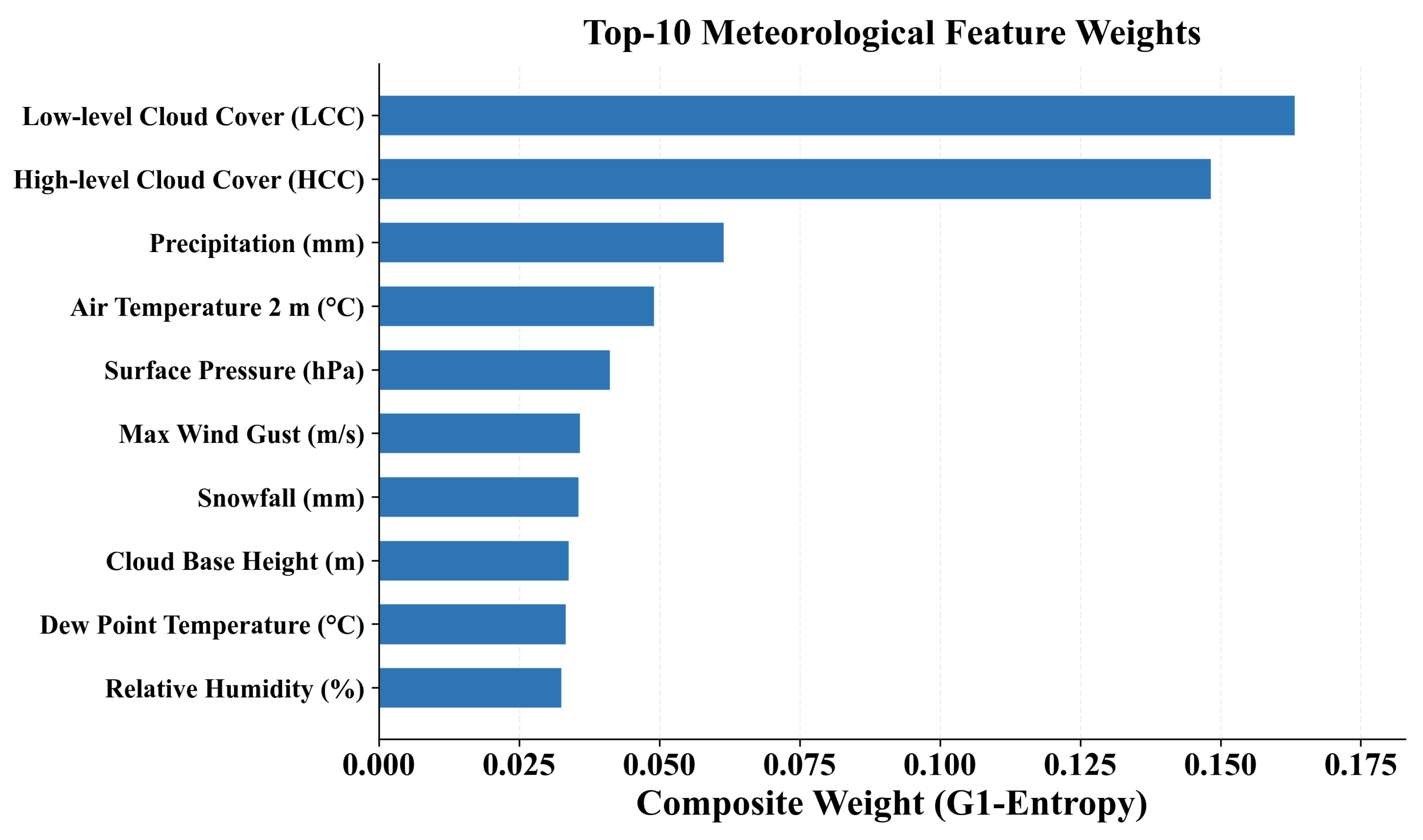
The G1–entropy composite weighting procedure was applied to quantify the relative importance of all 34 meteorological factors. Subjective weights were established through the G1 method by eliciting structured expert judgments on factor significance and converting pairwise importance ratios into numerical weights. Objective weights were derived via the entropy weight method by measuring the degree of variability in each factor’s observed distribution, assigning higher weights to factors with greater discriminative dispersion. Combining these two weight sets through Lagrange-multiplier optimization yielded the final composite weights, which are presented in Table 2.

Table 2. Relative weights of weather predictors.

Indicator Layer	G1	Entropy Weight Method	Combined Weight
sea level pressure/hPa	0.0328	0.0060	0.00747
surface pressure/hPa	0.0427	0.0215	0.03451
air temperature at 2 m (°C)	0.1325	0.0139	0.06918
precipitation/mm	0.1722	0.0017	0.01131
snowfall/mm	0.0031	0.0006	0.00007
snow depth (mm of water equivalent)	0.0004	0.0006	0.00001
snow density/(kg/m3)	0.0003	0.0027	0.00003
surface temperature/°C	0.1204	0.0104	0.04721
dew point temperature/°C	0.0002	0.0731	0.00053
relative humidity/%	0.0860	0.0478	0.15498
evaporation/mm	0.0171	0.0677	0.04362
potential evaporation/mm	0.0022	0.1213	0.01006
meridional wind speed (V, m/s)	0.0008	0.0029	0.00008
zonal wind speed (U, m/s)	0.0005	0.0073	0.00014
maximum wind gust (past hour, m/s)	0.0004	0.0034	0.00005
cloud base height/m	0.0614	0.0014	0.00333
low-level cloud cover (LCC)	0.0111	0.0487	0.02038
mid-level cloud cover (MCC)	0.0101	0.0294	0.01117
high-level cloud cover (HCC)	0.0072	0.1776	0.04827
total cloud cover (TCC)	0.0155	0.2309	0.13529
total solar radiation (downward, J/m2)	0.0274	0.0139	0.01430
net solar radiation (net, J/m2)	0.0016	0.0146	0.00086
direct radiation/(J/m2)	0.0010	0.0077	0.00028
ultraviolet intensity/(J/m2)	0.0512	0.0102	0.01967
runoff/mm	0.0048	0.0007	0.00013
surface runoff/mm	0.0037	0.0006	0.00008
subsurface runoff/mm	0.0037	0.0005	0.00006
thunderstorm probability (TT, K)	0.0002	0.0239	0.00016
K-index/K	0.1894	0.0513	0.36671
Convective Available Potential Energy (CAPE)/(J/kg)	0.0001	0.0079	0.00004

5.3. Visualization Analysis of Feature Extraction

The feature-extraction model was implemented in Python (version: 3.12) using scikit-learn, TensorFlow/Keras, and XGBoost. After systematic grid search over layer widths, sparsity coefficients, and learning rates, the optimal SAE hyperparameter configuration was determined and is detailed in Table 3.

Table 3. Optimized SAE hyperparameter settings.

Parameter	Value
network architecture (encoder)	$\mathrm{Input}\left(34\right)\to 24\to 18\to \mathrm{Output}\left(14\right)$
regularization type	KL-divergence sparsity penalty
sparsity target ($\rho$)	0.05
sparsity weight ($\beta$)	0.1
activation function	sigmoid (hidden), linear (output)
optimizer	Adam (${\beta }_1=0.9$, ${\beta }_2=0.999$)
learning rate	$1\times {10}^{-3}$
maximum iterations	500
batch size	32

According to the actual data of power grid accidents (incidents), different natural disaster scenarios are independent of each other. Each event corresponds to only one disaster type (e.g., lightning damage does not occur simultaneously with wind damage), and there are no concurrent occurrences of various meteorological disaster scenarios. Therefore, there is no intersection among the aforementioned meteorological disasters.

This classification system categorizes meteorological scenarios into seven disaster types: lightning damage, wind damage, typhoon, heavy rain, snow disaster, ice covering, and pollution flashover. The labels and corresponding codes for each scenario are presented in Table 4.

Table 4. Categorical taxonomy of weather patterns.

Meteorological Disaster Scenario	Scenario Label	Scenario Code
lightning damage	1	1000000
wind damage	2	0100000
typhoon	3	0010000
heavy rain	4	0001000
snow disaster	5	0000100
ice covering	6	0000010
pollution flashover	7	0000001

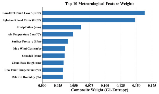
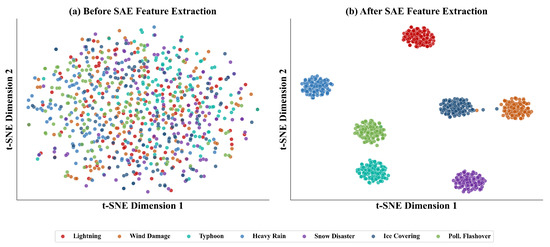
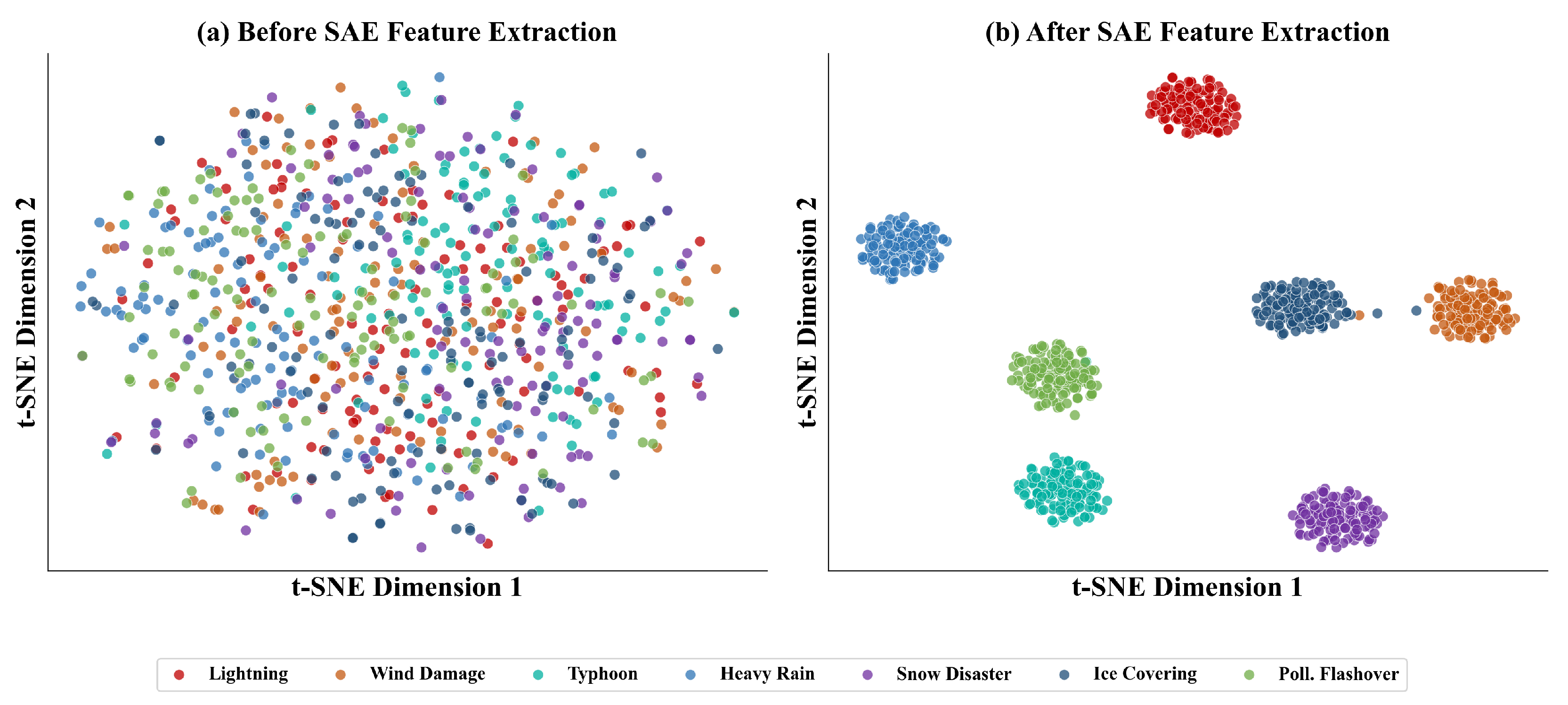
Raw collected data often possess high-dimensional attributes. Without dimensionality reduction or feature extraction processing, the data tends to exhibit a disordered distribution. The sparse autoencoder (SAE) adopted in this study uses a stacked architecture ($34\to 24\to 18\to 14$) with a KL-divergence sparsity penalty to achieve unsupervised representation of features. The preliminary training process has been successfully implemented, during which the data undergoes the encoding and decoding stages of the neural network. Following supervised fine-tuning, the 14-dimensional SAE-encoded representations exhibit markedly improved inter-class separability: feature boundaries become more distinguishable, intra-class clusters grow more compact, and inter-class distances are significantly enlarged Figure 6. These improvements reflect the discriminative sharpening achieved by the SAE encoder itself; no additional classification layer is interposed at this stage, as the final prediction is performed exclusively by the BP+XGBoost soft-voting ensemble described in Section 4.4. The visualization results are presented in Figure 7.

Figure 6. Top-10 meteorological feature composite weights (G1–Entropy combined method).

Figure 7. T-SNE visualization of SAE-encoded features: (a) before augmentation showing indistinguishable inter-class overlap, and (b) after SMOTE augmentation with markedly improved class separation.

5.4. Early Warning Model Based on Meteorological Scene Features

This study implements the complete early warning pipeline in Python (scikit-learn, XGBoost, TensorFlow/Keras). The SMOTE-balanced training set was used to train the SAE and the BP+XGBoost ensemble; the held-out test set was used exclusively for evaluation. The per-class training accuracy is reported in Table 5.

Table 5. Per-class training accuracy of the proposed model (augmented training set).

Meteorological Disaster Scenario	Training Accuracy (%)	Overall (%)
lightning damage	96.5	97.31
wind damage	95.8
typhoon	98.1
heavy rain	97.4
snow disaster	99.2
ice covering	99.5
pollution flashover	98.7

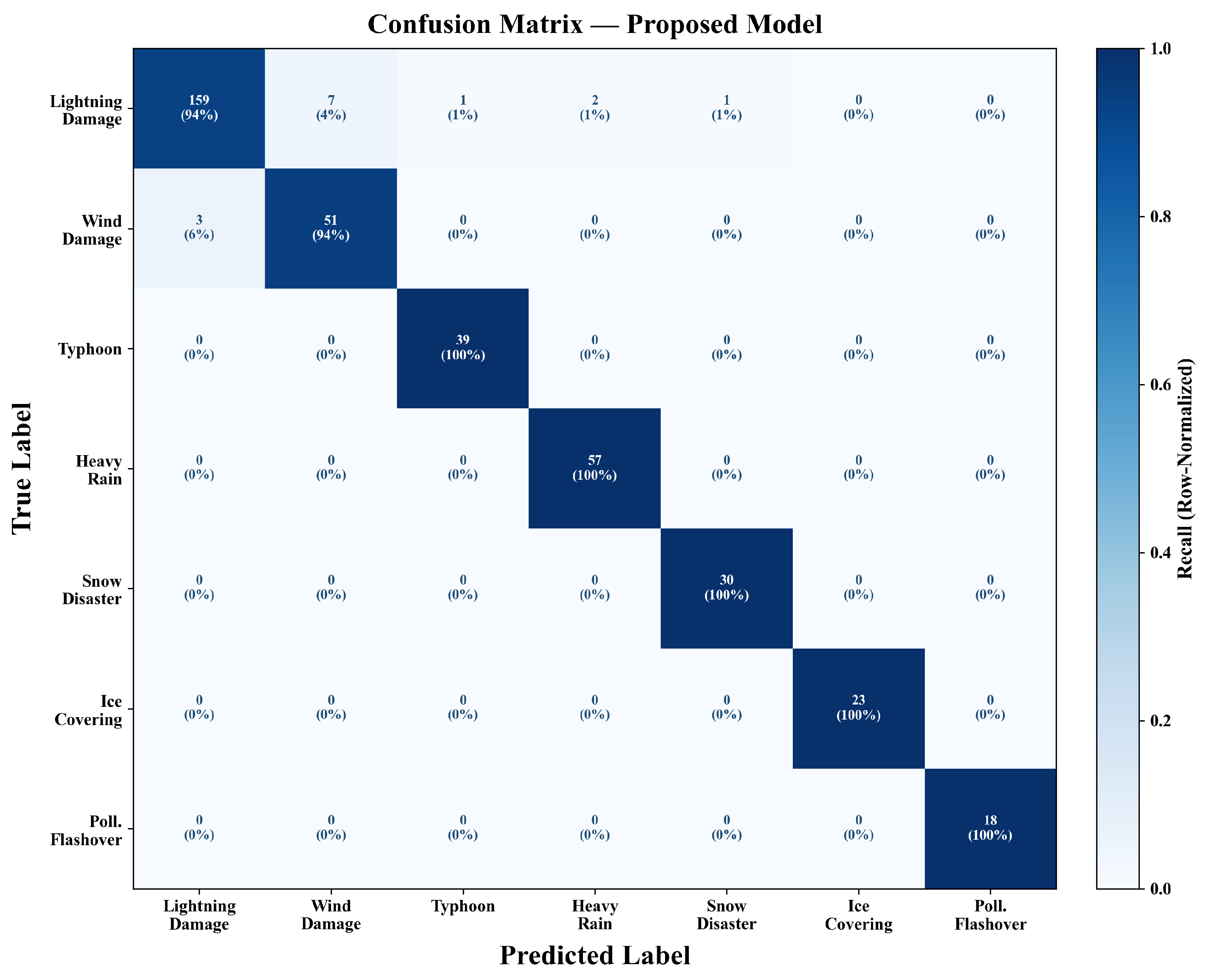
As shown in Table 5, the overall training accuracy reached 97.31%. The per-class test recall, precision, and F1-score are reported in the comprehensive evaluation table, which shows an overall test accuracy of 96.42%. The 0.89 percentage point gap between training and test accuracy confirms that the model generalizes well without significant overfitting. Lightning damage and wind damage are the two categories with the lowest test recall (93.53% and 94.44%, respectively), consistent with the feature-overlap analysis in Section 4.4. All other five categories achieved 100% recall on the test set, confirming that the SAE+G1–Entropy+SMOTE+BP⊕XGBoost pipeline achieves reliable early warning across all seven disaster scenarios.

5.5. Analysis of Error Characteristics of Disaster Early Warning Models Using Multi-Dimensional Assessment

A systematic analysis of the prediction results from the proposed early warning model reveals that model errors exhibit a pronounced type-concentrated characteristic. The bidirectional cross-category confusion between wind damage and lightning damage constitutes the primary error source in the current early warning system. Among all the misclassified lightning damage samples, 71% were misclassified specifically as wind damage (rather than any other category), significantly exceeding the inter-class confusion rates for all the other disaster type pairs. Likewise, among all the misclassified wind damage samples, 67% were misclassified as lightning damage. These proportions confirm that lightning–wind confusion dominates the model’s error budget, while confusion among other category pairs is negligible.

Through error analysis, this study reveals a key issue in power grid fault diagnosis: there is significant overlap between lightning damage and wind damage in the feature space, leading to systematic discrimination bias in the diagnostic system and severely affecting diagnostic accuracy. As shown in Table 6 and Table 7, key meteorological factors such as maximum thunderstorm probability, K-index, and relative humidity exhibit dual importance in the prediction of both disaster types. Among these, the K-index ranks second in both wind damage and lightning damage prediction, while maximum thunderstorm probability ranks first in lightning damage but sixth in wind damage. This high degree of factor sharing constitutes the physical basis for the misclassification phenomenon, making it difficult for the model to establish a clear decision boundary in the feature overlap region.

Table 6. Importance ranking of meteorological factors for lightning damage.

Independent Variable	Importance	Normalized (%)
max thunderstorm probability	0.063	100.0
K-index	0.062	98.6
mid-level cloud cover	0.062	98.4
relative humidity	0.052	83.2
surface temperature	0.051	81.7
zonal wind speed	0.048	76.5

Table 7. Importance Ranking of Meteorological Factors for Wind Damage.

Independent Variable	Importance	Normalized (%)
wind speed at 10 m	0.069	100.0
K-index	0.067	96.3
relative humidity	0.056	81.2
2 m air temperature	0.055	79.4
max wind gust	0.051	73.6
thunderstorm probability	0.050	72.7

From a physical mechanism perspective, this feature overlap originates from the fact that the accumulation of atmospheric instability energy under severe convection conditions can induce both thunderstorms and strong winds. This phenomenon of homologous anomalies with different manifestations poses an inherent discrimination difficulty for diagnostic systems based on traditional meteorological parameters. In the proposed model, lightning damage achieved 93.53% recall and wind damage achieved 94.44% recall; the remaining misclassified samples were predominantly confused with each other (71% and 67% of the respective error budgets), directly reflecting this physical overlap as the dominant residual error source.

Through the analysis of meteorological factor importance and comparison of key parameters, this study reveals the formation mechanism of prediction errors between wind damage and lightning damage. The K-index ranks second in the prediction of both disaster types, indicating that severe convection development potential serves as their common physical basis, reflecting the essential correlation in the occurrence conditions of the two disaster types, and constitutes the fundamental cause of model confusion.

Maximum thunderstorm probability ranks first in lightning damage prediction and also sixth in wind damage prediction, indicating a close association between thunderstorm activity and wind damage events, which may originate from the downdrafts accompanying severe thunderstorms or the circulation patterns favorable for the development of both phenomena. Relative humidity exhibits stable importance in both wind damage (third) and lightning damage (fourth) predictions, reflecting the universal constraint of moisture conditions on the formation of both disaster types.

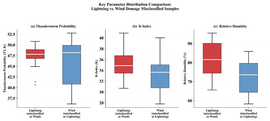
Based on the comparative analysis in Table 8, there is a significant overlap in the distribution intervals of thunderstorm probability, K-index, and relative humidity between lightning damage samples misclassified as wind damage and wind damage samples misclassified as lightning damage, further confirming the discrimination difficulty caused by feature similarity.

Table 8. Key meteorological parameters of selected misclassified samples (nine paired cases).

Thunderstorm Prob. (%)		K-Index		Rel. Humidity (%)
Lgtn → Wind	Wind → Lgtn	Lgtn → Wind	Wind → Lgtn	Lgtn → Wind	Wind → Lgtn
44.96	39.75	37.59	34.45	75.43	64.60
40.68	41.33	36.74	35.23	90.95	83.86
47.63	41.76	38.55	34.77	73.96	69.91
50.79	48.02	31.74	31.42	88.46	79.95
49.23	48.69	34.38	34.40	74.49	73.61
47.98	40.98	34.74	30.79	91.65	85.84
48.54	41.02	35.83	35.08	68.70	75.66
47.61	49.94	34.36	35.83	94.16	59.88
45.96	49.97	32.22	30.79	83.44	67.18

Lgtn → Wind: lightning damage sample misclassified as wind damage; Wind → Lgtn: wind damage sample misclassified as lightning damage. Each row represents one paired misclassified sample.

Systematic statistical analysis of misclassified samples (Table 8, Figure 8) reveals that lightning damage samples misclassified as wind damage and wind damage samples misclassified as lightning damage exhibit significant overlap in the distribution intervals of all three key meteorological parameters. This high degree of parameter-space overlap not only explains the intrinsic physical correlation between the two disaster types but also directly identifies the essential cause of the remaining prediction errors. When these core meteorological factors simultaneously reach critical thresholds, the model cannot establish a clear classification boundary in the feature space. This finding provides a clear direction for subsequent improvement: developing multi-parameter integrated analysis schemes, strengthening spatiotemporal feature extraction, and refining decision boundaries through threshold optimization.

Figure 8. Box-plot comparison of key meteorological parameters (thunderstorm probability, K-index, relative humidity) between lightning damage samples misclassified as wind damage and wind damage samples misclassified as lightning damage.

The foregoing analysis confirms that bidirectional misclassification between wind damage and lightning damage constitutes the dominant source of residual prediction errors, rooted in the shared atmospheric instability signatures of severe convective weather. Because classical single-threshold methods are unable to resolve the complex multi-factor interactions that simultaneously produce both thunderstorm activity and strong surface winds, the proposed model reaches its performance ceiling precisely in this physically ambiguous region of feature space. These findings point to concrete improvement directions: multi-parameter integrated decision schemes that jointly consider convective indices, moisture fields, and wind shear; enhanced spatiotemporal feature extraction to capture the evolution of synoptic-scale patterns preceding each event; and adaptive threshold optimization that accounts for the asymmetric cost of misclassifying severe events.

Compared with Artemchuk et al. [31], who proposed a Unified Resilience Model (URM) based on deep learning to assess the operational fidelity of batteries and energy storage devices under weather-induced stress, the present study addresses a fundamentally different problem: seven-class meteorological fault-type classification across a regional 110–500 kV transmission network, which necessitates distinct preprocessing strategies—including sparse-autoencoder feature extraction and SMOTE oversampling—suited to high-dimensional tabular fault records. Prieto-Godino et al. [32] predicted daily weather-related outage incidences in large-scale Spanish distribution grids using a five-architecture deep learning ensemble with optimization-based feature selection; their approach benefits from a large volume of daily aggregated records, whereas the present study targets high-voltage transmission events with an order-of-magnitude smaller dataset (1955 samples), motivating the lightweight SAE pipeline over large-ensemble designs. Both studies shared the broader goal of leveraging meteorological information for power-system safety, yet operated in complementary problem settings—resilience assessment versus fault-type classification, distribution versus transmission, binary prediction versus seven-class discriminative modeling—confirming that the proposed framework fills a distinct and underexplored niche in the literature.

5.6. Comparative Evaluation and Ablation Study

To rigorously validate the proposed framework, we conducted a systematic comparative evaluation against classical and deep-learning baselines and six ablation variants using the leakage-free seven-step experimental protocol (Section 4.1). All our experiments shared the same stratified 80/20 train–test split and were evaluated on the held-out test set.

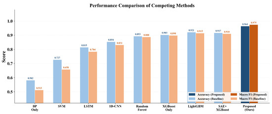
Table 9 and Figure 9 summarize the overall performance of the nine competing methods under the same leakage-free protocol. The proposed model achieved accuracy $=96.42\%$ and macro F1 $=97.46\%$, surpassing all the baselines. Among the classical methods, SVM (RBF kernel, $C=1.5$) reached only 72.68% accuracy and Random Forest (200 trees) achieved 89.31%, reflecting the limitations of these approaches on high-dimensional, class-imbalanced data. The deep-learning baselines—an LSTM network (two layers, hidden size 64, treating the 34 features as a temporal sequence, 81.47%) and a 1D-CNN (two Conv1D layers with 64/128 filters and GlobalAveragePooling, 85.38%)—were included as standard reference architectures, though neither was optimized for static tabular input. Among the gradient-boosting methods, XGBoost without SAE-encoded features reached 90.26%, and LightGBM [33] (leaf-wise growth, 200 trees, learning rate 0.05, ${𝓁}_2=1.0$) achieved 92.15%, outperforming plain XGBoost by 1.89 percentage points while still falling 4.27 points below the full proposed framework. The partial-ensemble variant SAE+XGBoost (without the BP branch) yielded 91.68%, confirming that SAE-based feature extraction provides a meaningful gain before XGBoost classification, and that the full soft-voting ensemble is required to achieve peak performance.

Table 9. Performance comparison of the proposed model versus competing baselines. The bold is the best.

Model	Accuracy (%)	Macro P (%)	Macro R (%)	Macro F1 (%)
BP only	58.19	57.84	55.62	51.27
SVM (RBF) [34]	72.68	71.43	69.27	65.81
LSTM [35]	81.47	80.93	80.14	78.43
1D-CNN [20]	85.38	84.71	84.06	83.12
Random Forest [36]	89.31	88.93	89.47	88.76
XGBoost only [37]	90.26	90.11	89.85	89.83
LightGBM [33]	92.15	91.87	91.54	91.47
SAE+XGBoost (no BP)	91.68	91.34	91.07	91.02
proposed (full)	96.42	96.71	98.28	97.46

Figure 9. Model comparison bar chart (accuracy and macro F1).

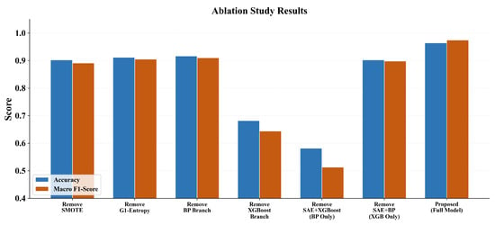
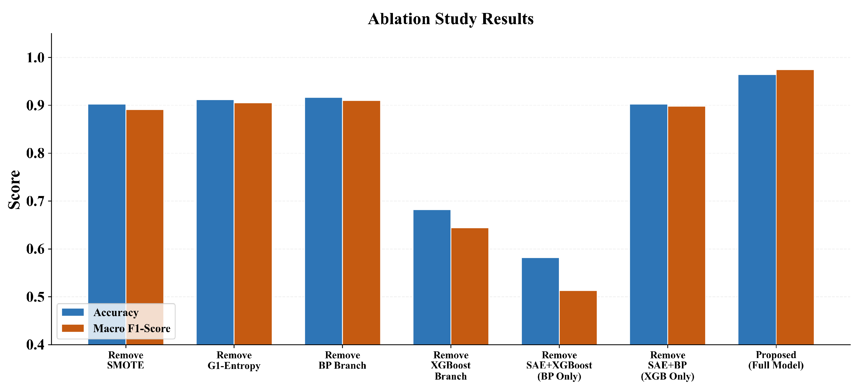
Table 10 and Figure 10 quantifies the contribution of each component relative to the full model. Removing the XGBoost branch (SAE+BP only) caused the largest degradation ($\Delta$Acc $=-28.25\%$, $\Delta$F1 $=-33.03\%$), confirming its dominant role. Removing SMOTE reduced Acc by 6.16% and F1 by 8.34%, validating the oversampling contribution. Removing G1–entropy weighting reduced F1 by 6.91%, confirming the value of composite feature weighting. Even LightGBM [33], one of the strongest single-model baselines, fell 4.27 percentage points below the proposed framework in accuracy and 5.99 points in macro F1, demonstrating the additive value of the full SAE + G1–Entropy + SMOTE + BP⊕XGBoost pipeline.

Table 10. Ablation study: degradation relative to the full proposed model.

Variant	Acc (%)	Macro F1 (%)	$\mathbf{\Delta }$Acc	$\mathbf{\Delta }$F1
proposed (full)	96.42	97.46	—	—
remove SMOTE	90.26	89.12	$-6.16$	$-8.34$
remove G1–Entropy	91.21	90.55	$-5.21$	$-6.91$
remove BP branch (SAE+XGBoost)	91.68	91.02	$-4.74$	$-6.44$
remove XGBoost branch (SAE+BP)	68.17	64.43	$-28.25$	$-33.03$
remove SAE (XGBoost only)	90.26	89.83	$-6.16$	$-7.63$
remove SAE (BP only)	58.19	51.27	$-38.23$	$-46.19$

Figure 10. Ablation study: accuracy and F1-score for each model variant.

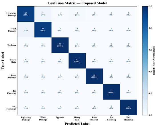
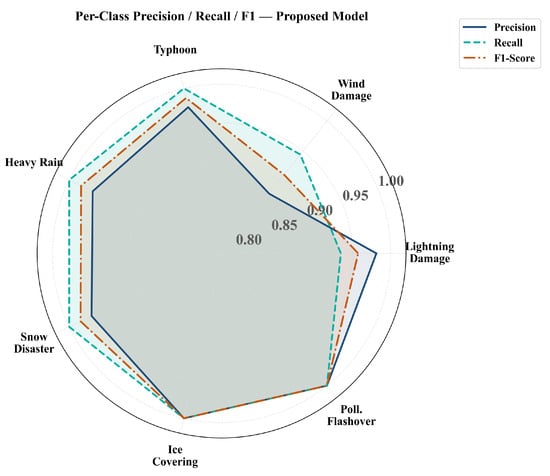
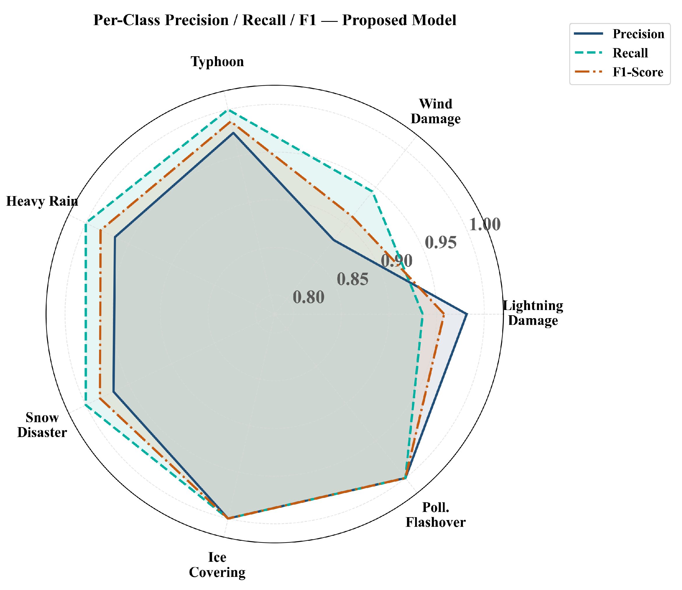
Table 11 and Figure 11 reports precision, recall, and F1-score for each of the seven disaster categories. All classes except lightning damage and wind damage achieved F1 $\ge 98\%$. The relatively lower performance of lightning damage and wind damage confirms the physical overlap identified in the error-analysis subsection (Figure 12).

Table 11. Per-class precision, recall, and F1-score of the proposed model. The bold is the best.

Disaster Category	Precision (%)	Recall (%)	F1-Score (%)
lightning damage	98.13	93.53	95.77
wind damage	87.93	94.44	91.07
typhoon	97.50	100.00	98.73
heavy rain	96.59	100.00	98.28
snow disaster	96.77	100.00	98.36
ice covering	100.00	100.00	100.00
pollution flashover	100.00	100.00	100.00
Macro Average	96.71	98.28	97.46
Weighted Average	97.19	96.42	96.43

Figure 11. Confusion matrix (row-normalized) of the proposed model on the test set.

Figure 12. Radar chart of per-class precision, recall, and F1-score.

The ablation and per-class results together illuminate the mechanism underlying the ensemble’s advantage. As Table 10 shows, removing the BP branch reduced macro F1 by 6.44 percentage points while reducing accuracy by only 4.74 points; this asymmetry indicates that BP’s contribution was concentrated disproportionately on the minority categories, where macro F1 was the more sensitive metric. Table 11 corroborates this: pollution flashover and ice covering—the two smallest categories in the training set—both achieved F1 $=100\%$ in the full ensemble, a result that neither branch achieved alone. The complementarity between the two branches arose from their distinct inductive biases: XGBoost’s tree-ensemble structure yielded robust discrimination on the data-rich majority classes, while BP’s gradient-based optimization provided smoother class-boundary calibration that benefited the rarer categories. The 1:1 soft-voting scheme therefore achieved macro F1 of 97.46%, which exceeded what either branch could attain individually.

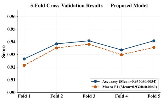
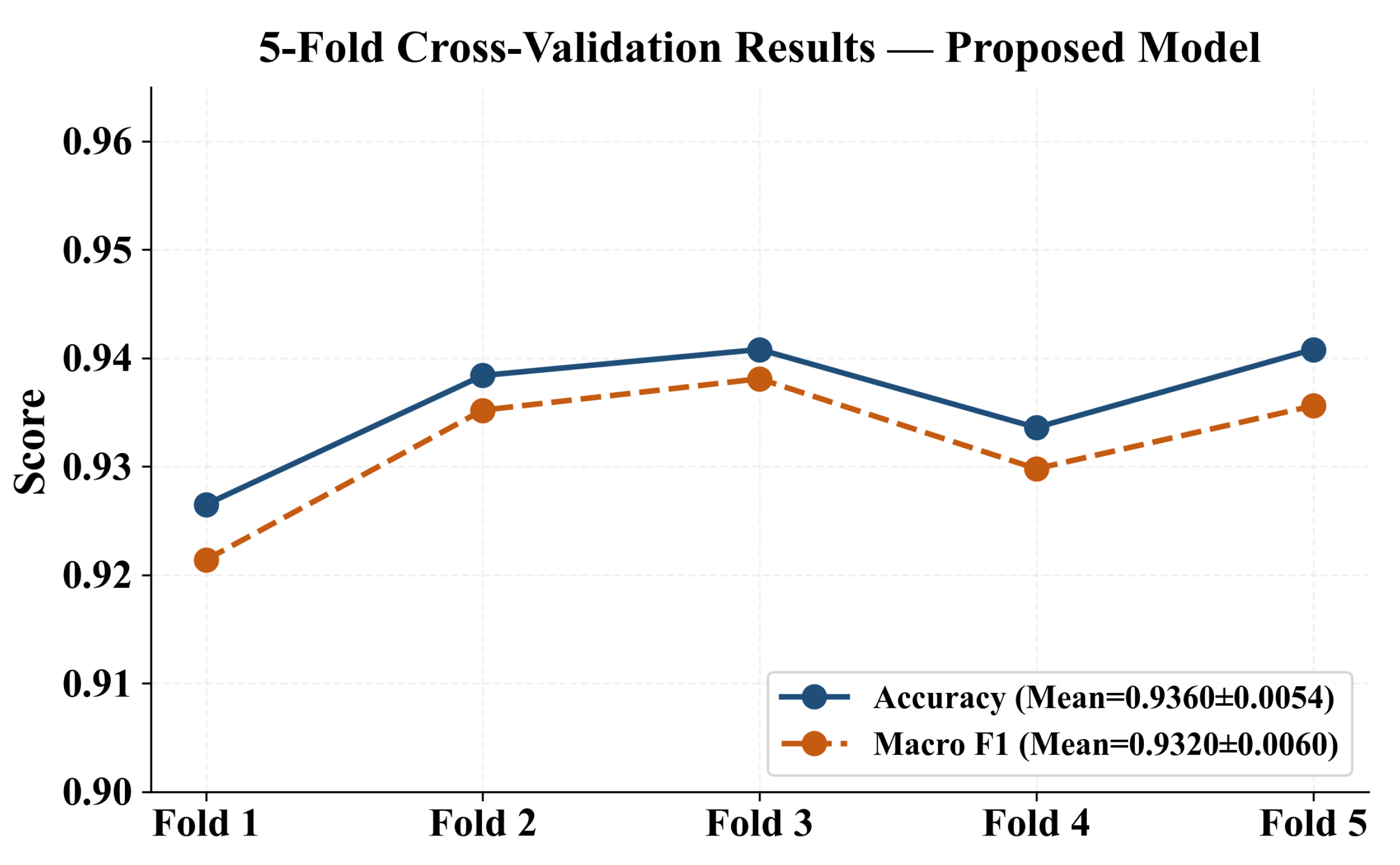
To confirm that the reported results were not an artifact of a favorable random split, a five-fold stratified cross-validation (CV) was conducted exclusively on the training partition (1564 samples) obtained from the initial 80/20 stratified split (Figure 13). Within each fold, SMOTE oversampling was applied independently to the training subset of that fold only; the validation subset remained free of any synthetic augmentation throughout, consistent with the leakage-free protocol established in Section 4.1. Table 12 reports the fold-level and aggregate results.

Figure 13. Five-fold cross-validation accuracy and F1-score per fold.

Table 12. Five-fold stratified cross-validation results. The bold is the best.

Fold	Accuracy (%)	Macro F1 (%)
Fold 1	92.65	92.14
Fold 2	93.84	93.52
Fold 3	94.08	93.81
Fold 4	93.36	92.98
Fold 5	94.08	93.56
Mean ± SD	93.60 ± 0.54	93.20 ± 0.60

The low standard deviations (Acc: $\pm 0.54\%$, F1: $\pm 0.60\%$) confirm that the model generalizes consistently across different data subsets and that the 80/20 hold-out result (Acc $=96.42\%$) is representative.

5.7. Temporal Validation

To address the temporal generalization concern raised in the review, a temporal validation experiment was conducted in which the model was trained exclusively on fault records from 2013–2018 and evaluated on records from 2019–2022. This protocol closely resembles real-world operational deployment, where predictions for future events must rely solely on historical data. All preprocessing steps—normalization, G1–entropy composite weighting, SMOTE oversampling, and SAE training—were applied to the 2013–2018 training partition only; the 2019–2022 test set was never touched during any fitting stage. Because SMOTE was confined to the training partition, no synthetic sample derived from post-2018 instances could contaminate the model, preserving the temporal integrity of the evaluation.

Table 13 reports per-class and macro-average precision, recall, and F1-score under this temporal split. The overall accuracy reached 91.57% and macro F1 reached 91.92%. Lightning damage retained the highest individual F1 (97.14%), confirming that the dominant disaster type is robustly captured across time periods. Wind damage recorded the lowest F1 (88.57%), consistent with the physical feature overlap between lightning and wind events analyzed in Section 4.4. All seven categories achieved F1 $\ge 88\%$, demonstrating that the proposed framework maintains reliable early warning capability in a time-ordered evaluation setting and that the meteorological–fault mapping is temporally stable over the 2013–2022 study period.

Table 13. Per-class metrics under temporal split (train: 2013–2018; test: 2019–2022). The bold is the best.

Disaster Category	Precision (%)	Recall (%)	F1-Score (%)
lightning damage	96.40	97.89	97.14
wind damage	86.49	90.74	88.57
typhoon	92.86	90.48	91.67
heavy rain	94.12	90.57	92.31
snow disaster	91.43	91.43	91.43
ice covering	89.47	89.47	89.47
pollution flashover	92.86	92.86	92.86
Macro Average	91.95	91.92	91.92

5.8. Limitations and Future Work

The present study has several limitations that should be acknowledged. In terms of geographic scope, the model was trained on data from a single regional grid in East China; direct application to other climatic zones or grid configurations would require retraining on locally collected fault records. Regarding voltage coverage, only events at 110 kV, 220 kV, and 500 kV transmission levels are included, and applicability to medium-voltage distribution networks remains untested. The model also does not account for the rapid evolution of grid topology driven by renewable energy integration; periodic retraining on a rolling time window is therefore recommended as new fault records accumulate to maintain predictive accuracy under changing operating conditions. The G1 subjective component of the composite weighting scheme reflects domain knowledge about meteorological factor importance and is expected to remain stable unless the input feature set is fundamentally restructured; in practice, only the entropy-weight component needs to be recomputed automatically when new fault data are incorporated into a rolling training window, keeping the expert-elicitation overhead minimal. Furthermore, model performance is bounded by the accuracy of historical event labeling: mislabeled records in minority disaster categories directly impair recall and cannot be corrected without manual re-annotation. Finally, the SMOTE oversampling strategy relies on linear interpolation in feature space, which may not fully capture the non-linear manifold structure of rare disaster categories such as pollution flashover. Future work will explore transfer-learning adaptation to new geographic regions, online learning with streaming fault data, and incorporation of spatial grid-topology features to further improve discrimination between physically similar disaster categories. A temporal-split validation using records from 2013–2018 for training and 2019–2022 for testing has been conducted and is reported in Section 4.1.

6. Conclusions

This paper proposes a power grid meteorological fault early warning method based on the synergistic optimization of a sparse autoencoder and ensemble learning. A corrected, leakage-free experimental protocol was established, and comprehensive comparative and ablation experiments validated the contribution of each component. The proposed framework achieved 96.42% accuracy and a 97.46% macro F1-score on a regional grid dataset covering 110 kV, 220 kV, and 500 kV voltage levels (2013–2022).

A core methodological contribution is the leakage-free seven-step experimental protocol, which confines SMOTE oversampling exclusively to the training partition while keeping the test set untouched throughout the entire pipeline. The robustness of this design was confirmed by five-fold cross-validation, which yielded a mean accuracy of $93.60\%\pm 0.54\%$ and a mean macro F1 of $93.20\%\pm 0.60\%$, demonstrating stable generalization across different data subsets. The G1–entropy composite weighting method (validated by a five-expert Delphi process with Kendall $W=0.81$, $p<0.01$) quantifies the relative importance of meteorological factors by integrating expert judgment with information-theoretic objective weights, substantially improving model convergence efficiency and discriminative capacity; ablation experiments confirmed that removing this weighting reduces macro F1 by 6.91 percentage points. The stacked SAE ($34\to 24\to 18\to 14$ with KL-divergence sparsity penalty) extracts compact and discriminative meteorological feature representations without requiring labeled samples, and the subsequent soft-voting BP+XGBoost ensemble outperformed all the evaluated baselines, including SVM (72.68%), Random Forest (89.31%), and standalone XGBoost (90.26%). Ablation analysis further revealed that the XGBoost branch was the dominant contributor to ensemble performance—its removal degraded accuracy by 28.25% and macro F1 by 33.03%—while the BP branch provided complementary minority-class calibration, accounting for a 6.44-percentage-point reduction in macro F1 when excluded. Through confusion matrix decomposition and feature importance ranking, the bidirectional misclassification between wind damage and lightning damage was identified as the dominant residual error source, rooted in the shared atmospheric instability signatures of severe convective weather. Despite this physical overlap, the proposed model achieved F1 $=95.77\%$ for lightning damage and F1 $=91.07\%$ for wind damage, providing a theoretical basis for further threshold optimization and multi-parameter discrimination strategies in future operational warning systems.

References

- Feng, X.; Guo, D.; Ye, M. DMoE-LLM: A Dual-Branch Mixture-of-Experts Framework with Large Language Models for Wind Power Forecasting. Expert Syst. Appl. 2026, 325, 132637. [Google Scholar] [CrossRef] [Scilit]
- Cao, P.; Huang, M.; Wang, Y. Electromagnetic transients analysis and indirect traveling wave fault location for ground wires of AC transmission line amid de-icing. Power Syst. Prot. Control 2023, 51, 11–21. [Google Scholar]
- Wu, R.; Li, X.; Bin, D. Network attack identification model of smart grid based on XGBoost algorithm. Electr. Meas. Instrum. 2023, 60, 64–86. [Google Scholar]
- Liang, Y.; Ren, Y.; Yu, J.; Zha, W. Current Trajectory Image-Based Protection Algorithm for Transmission Lines Connected to MMC-HVDC Stations Using CA-CNN. Prot. Control Mod. Power Syst. 2023, 8, 6. [Google Scholar] [CrossRef] [Scilit]
- Liu, K.; Zhan, H.; Tan, Y. High impedance grounding fault detection in distribution network based on improved extreme learning machine. Power Syst. Technol. 2023, 47, 1186–1896. [Google Scholar]
- Zuo, L.; Xie, K. Research on the human-involved risk coupling and effectiveness of intelligent decoupling technologies of safety risk in power system construction and operation. Reliab. Eng. Syst. Saf. 2026, 270, 112180. [Google Scholar] [CrossRef] [Scilit]
- Luo, C.; Yu, K.; Zeng, X. Low voltage arc fault identification method based on high frequency reconstructed signal and Bayes-XGBoost. Power Syst. Prot. Control 2023, 51, 91–101. [Google Scholar]
- Feng, X.; Liu, L.; Ye, M.; Mašek, O.; Gouda, S.; Chang, K.; Wang, X.; Huang, Q. Unveiling and interpreting the relationships among multi-pollutant emission factors in municipal solid waste incineration by machine learning. Waste Manag. 2026, 210, 115256. [Google Scholar] [CrossRef] [Scilit]
- Liu, W.; Ren, C.; Xu, Y. PV Generation Forecasting with Missing Input Data: A Super-Resolution Perception Approach. IEEE Trans. Sustain. Energy 2021, 12, 1493–1496. [Google Scholar] [CrossRef] [Scilit]
- Li, Y.; Song, L.; Zhang, S.; Kraus, L.; Adcox, T.; Willardson, R.; Komandur, A.; Lu, N. A TCN-Based Hybrid Forecasting Framework for Hours-Ahead Utility-Scale PV Forecasting. IEEE Trans. Smart Grid 2023, 14, 4073–4085. [Google Scholar] [CrossRef] [Scilit]
- Trip, S.; Persis, C. Distributed Optimal Load Frequency Control with Non-Passive Dynamics. IEEE Trans. Control Netw. Syst. 2018, 5, 1232–1244. [Google Scholar] [CrossRef] [Scilit]
- Li, D.; Gong, Y.; Shen, S.; Feng, G. Research and Design of Meteorological Disaster Early Warning System for Power Grid Based on Big Data Technology. In Proceedings of the 2020 Asia Energy and Electrical Engineering Symposium (AEEES); IEEE: Piscataway, NJ, USA, 2020; pp. 658–662. [Google Scholar]
- Perninge, M.; Söder, L. A Stochastic Control Approach to Manage Operational Risk in Power Systems. IEEE Trans. Power Syst. 2012, 27, 1021–1031. [Google Scholar] [CrossRef] [Scilit]
- Guo, M.; Liu, W.; Gao, J.; Chen, D. A Data-Enhanced High Impedance Fault Detection Method Under Imbalanced Sample Scenarios in Distribution Networks. IEEE Trans. Ind. Appl. 2023, 59, 4720–4733. [Google Scholar] [CrossRef] [Scilit]
- Zhang, Q.; Chen, Y.; Jin, L.; Chen, S. Intelligent identification and reasoning of causal relationships in texts on power production accidents. Adv. Eng. Inform. 2026, 69, 103977. [Google Scholar] [CrossRef] [Scilit]
- Liu, K.; Ye, X.; Li, Z. Detection method of high resistance grounding fault in distribution network based on multi-resolution wavelet transform. High Volt. Eng. 2023, 49, 4247–4256. [Google Scholar]
- Sun, Y.; Wu, J.; Zhang, J.; Xiong, Y.; Liu, X.; Bai, Y. Scenario construction and vulnerability assessment of natural hazards-triggered power grid accidents. J. Saf. Sci. Resil. 2024, 5, 498–511. [Google Scholar] [CrossRef] [Scilit]
- Hu, L.; Cong, W.; Xu, A. Power grid meteorological fault early warning method based on deep sparse autoencoder network and scene classifier. Power Syst. Prot. Control 2022, 50, 68–78. [Google Scholar]
- Li, B.; Thomas, G.; Williams, D. Detection of Ice on Power Cables Based on Image Texture Features. IEEE Trans. Instrum. Meas. 2018, 67, 497–504. [Google Scholar] [CrossRef] [Scilit]
- Zhang, D.; Zhang, X.; Sun, H. Fault diagnosis for AC/DC transmission system based on convolutional neural network. Autom. Electr. Power Syst. 2022, 46, 132–145. [Google Scholar]
- Xian, G.m. An identification method of malignant and benign liver tumors from ultrasonography based on GLCM texture features and fuzzy SVM. Expert Syst. Appl. 2010, 37, 6737–6741. [Google Scholar] [CrossRef] [Scilit]
- Zhang, Y.; Wu, Y.; Zhang, F.; Yao, X.; Liu, A.; Tang, L.; Mo, J. Application of power grid wind monitoring data in transmission line accident warning and handling affected by typhoon. Energy Rep. 2022, 8, 315–323. [Google Scholar] [CrossRef] [Scilit]
- Liu, Y.; Yang, D.; Lyu, J.; Li, J.; Li, Z.; Liu, M.; Liu, W.; Ren, Z.; Liu, H.; Yan, Y.; et al. Integrated micro thermoelectric devices with self-power supply and temperature monitoring: Design and application in power grid early warning. Appl. Therm. Eng. 2024, 247, 122922. [Google Scholar] [CrossRef] [Scilit]
- Wang, B.; Ma, F.; Ge, L.; Ma, H.; Wang, H.; Mohamed, M. Icing-EdgeNet: A Pruning Lightweight Edge Intelligent Method of Discriminative Driving Channel for Ice Thickness of Transmission Lines. IEEE Trans. Instrum. Meas. 2021, 70, 1–12. [Google Scholar] [CrossRef] [Scilit]
- Li, Q.; Xu, Y.; Chew, B.; Ding, H.; Zhao, G. An Integrated Missing-Data Tolerant Model for Probabilistic PV Power Generation Forecasting. IEEE Trans. Power Syst. 2022, 37, 4447–4459. [Google Scholar] [CrossRef] [Scilit]
- Yu, M.; Du, W.; Li, J.; Zhang, S.; Hu, J. Study on a comprehensive indicator and online classification of early warning of low frequency oscillation in power system. Eng. Appl. Artif. Intell. 2023, 124, 106592. [Google Scholar] [CrossRef] [Scilit]
- Ma, G.; Yue, X.; Gao, X.; Liu, F. Application of an improved sparrow search algorithm in BP network classification of strip steel surface defect images. Multimed. Tools Appl. 2023, 82, 14403–14439. [Google Scholar] [CrossRef] [Scilit]
- Gao, F.; Li, Q.; Ji, Y.; Ji, S.; Guo, J.; Sun, H.; Liu, Y.; Feng, S.; Wei, H.; Wang, N.; et al. EWNet: An early warning classification framework for smart grid based on local-to-global perception. Neurocomputing 2021, 443, 199–212. [Google Scholar] [CrossRef] [Scilit]
- Wu, J.; Li, L.; Shi, F.; Zhao, P.; Li, B. A two-stage power system frequency security multi-level early warning model with DS evidence theory as a combination strategy. Int. J. Electr. Power Energy Syst. 2022, 143, 108372. [Google Scholar] [CrossRef] [Scilit]
- Rao, C.; Liu, Y.; Goh, M. Credit risk assessment mechanism of personal auto loan based on PSO-XGBoost Model. Complex Intell. Syst. 2023, 9, 1391–1414. [Google Scholar] [CrossRef] [Scilit]
- Artemchuk, V.; Garbuz, I.; Jamil Alsayaydeh, J.A.; Shkarupylo, V.; Oliinyk, A.; Bin Yusof, M.F.; Herawan, S.G. Unified resilience model using deep learning for assessing power system performance. Heliyon 2025, 11, e42802. [Google Scholar] [CrossRef] [Scilit]
- Prieto-Godino, L.; Peláez-Rodríguez, C.; Pérez-Aracil, J.; Pastor-Soriano, J.; Salcedo-Sanz, S. Predicting weather-related power outages in large scale distribution grids with deep learning ensembles. Int. J. Electr. Power Energy Syst. 2025, 170, 110811. [Google Scholar] [CrossRef] [Scilit]
- Ke, G.; Meng, Q.; Finley, T.; Wang, T.; Chen, W.; Ma, W.; Ye, Q.; Liu, T.Y. LightGBM: A Highly Efficient Gradient Boosting Decision Tree. Adv. Neural Inf. Process. Syst. 2017, 30, 3146–3154. [Google Scholar]
- Cortes, C.; Vapnik, V. Support-vector networks. Mach. Learn. 1995, 20, 273–297. [Google Scholar] [CrossRef] [Scilit]
- Hochreiter, S.; Schmidhuber, J. Long Short-Term Memory. Neural Comput. 1997, 9, 1735–1780. [Google Scholar] [CrossRef] [Scilit] [PubMed]
- Breiman, L. Random forests. Mach. Learn. 2001, 45, 5–32. [Google Scholar] [CrossRef] [Scilit]
- Chen, T.; Guestrin, C. Xgboost: A scalable tree boosting system. In Proceedings of the 22nd ACM SIGKDD International Conference on Knowledge Discovery and Data Mining; Association for Computing Machinery: New York, NY, USA, 2016; pp. 785–794. [Google Scholar]
Disclaimer/Publisher’s Note: The statements, opinions and data contained in all publications are solely those of the individual author(s) and contributor(s) and not of MDPI and/or the editor(s). MDPI and/or the editor(s) disclaim responsibility for any injury to people or property resulting from any ideas, methods, instructions or products referred to in the content. |
© 2026 by the authors. Licensee MDPI, Basel, Switzerland. This article is an open access article distributed under the terms and conditions of the Creative Commons Attribution (CC BY) license.