Enhanced Renewable Energy Integration: A Comprehensive Framework for Grid Planning and Hybrid Power Plant Allocation

Abstract

Renewable energy sources play a crucial role in the urgent global pursuit of decarbonizing electricity systems. However, persistent grid congestion and lengthy planning approval processes remain the main barriers to the accelerated deployment of new green energy source capacities. Capitalizing on the synergies afforded by co-locating hybrid power plants—particularly those that harness temporally anti-correlated renewable sources such as wind and solar—behind a unified connection point presents a compelling opportunity. To this end, this paper pioneers a comprehensive planning framework for hybrid configurations, integrating transmission grid and renewable energy assets planning to include energy storage systems, wind, and solar energy capacities within a long-term planning horizon. A mixed-integer linear programming model is developed that considers both the technical and economic aspects of combined grid planning and hybrid power plant allocation. Additionally, the proposed framework incorporates the N − 1 contingency criterion, ensuring system reliability in the face of potential transmission line outages, thereby adding a layer of versatility and resilience to the approach. The model minimizes the net present value of costs, encompassing both capital and operational expenditures as well as curtailment costs. The efficacy of the proposed model is demonstrated through its implementation on the benchmark IEEE 24-bus RTS system, with findings underscoring the pivotal role of hybrid power plants in enabling cost-effective and rapid sustainable energy integration.

1. Introduction

In the ever-changing landscape of global energy, integrating Renewable Energy Sources (RESs) is pivotal for sustainability [1]. However, challenges like transmission line (TL) congestion and RES’ intermittent nature require a careful planning approach that maximizes the synergy between various RES along the planning horizon. To address these challenges, power systems operators are increasingly adopting ESSs due to market participation, dispatchable energy supply, reducing the uncertainty of RESs, and mitigating power quality concerns [2]. Moreover, expansion planning for transmission systems becomes crucial to accommodate rising electricity generation from RES and demand for electric vehicle adoption [3].

1.1. Literature Review

Much literature has been published on optimal planning strategies for grid-connected and standalone systems incorporating PV systems, Wind Turbines (WTs), and ESS technologies [4,5]. These studies primarily focus on capacity optimization for PV and ESS in grid-connected households, prosumers [6]. In addition to planning considerations, ongoing research efforts explore optimal daily operation strategies for these technologies through various approaches like data-driven and game theory frameworks [7,8,9]. These efforts offer valuable insights but fail to address several critical research gaps targeted in this paper: (i) neglecting long-term system resilience and grid component outage management in planning models, (ii) overlooking significant seasonal variations in RES generation and demand patterns for optimal operation and planning, (iii) oversimplifying economic analysis by using fixed values per MW or MWh without accounting for the varying cost components of each technology over the planning horizon, and (iv) assuming grid connection permissions for renewable assets without accounting for the bureaucratic processes and grid compatibility tests required in practice.

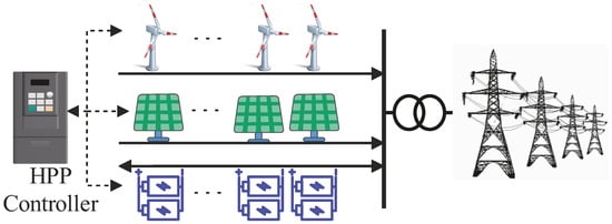
HPPs, incorporating multiple RES and/or storage technologies behind a single connection point [10], constitute a paradigm-shifting solution to expedite energy transition by offering substantial value to both plant owners and power systems. The inherent synergy between heterogeneous RESs, particularly the complementary nature of wind and solar resources—where their outputs are often negatively correlated—ensures more stable and predictable power generation by HPPs. This inherent synergy not only reduces intermittency but also allows for strategic dispatching in electricity markets, maximizing economic returns [11]. Furthermore, HPPs optimize the utilization of existing transmission infrastructure, eliminating the need for new transmission lines and substations while circumventing impediments associated with acquiring new planning and grid connection permissions. HPPs leverage economies of scope through shared grid connections, reduced land costs, and streamlined project planning resources [12,13,14]. Simulation studies emphasize their dual benefits: the ability to emulate the scheduling characteristics of conventional generators under varying weather conditions and maintain grid frequency stability [15]. Additionally, co-located ESS mitigates renewable energy curtailment due to grid constraints while enabling more uniform and efficient storage device operation [16,17]. Despite their potential, the complexity of HPPs’ design, coupled with high capital costs, necessitates advanced planning and control strategies to determine economically viable and reliable configurations. These considerations underscore the importance of continued research in HPP planning to unlock their full potential in the energy transition. The conceptual paradigm of HPPs, being contingent upon a single grid connection, is delineated in Figure 1.

Figure 1. Co-located grid connected HPP configuration.

Several studies have examined hybrid renewable systems in different contexts, such as grid-connected and islanded operational modes [18], rural electrification applications [19], PV–diesel system planning for remote areas [20], and multi-objective optimization frameworks that balance technical and economic trade-offs [21]. Others have investigated the comparative advantages of network expansion versus integrating hybrid systems [22]. While these works provide valuable insights into system sizing, operational strategies, and techno-economic evaluation, most are tailored to isolated systems (e.g., a village, some buildings) and do not address the simultaneous optimization of both siting and sizing in a large interconnected grid. Furthermore, they typically focus on either technical or economic aspects, oversimplifying the other dimension. Critically, all of them omit the explicit consideration of a shared grid connection point within the optimization model, which is the backbone of every definition of HPPs. Instead, they rely on conventional planning methods to determine sizing and siting first and only afterward explore the possibility of downsizing grid connection capacity. Moreover, to the best of the authors’ knowledge, no prior study has simultaneously incorporated all key planning aspects—namely transmission line expansion, sizing and siting of renewable and ESS assets, seasonal variations of renewable resources, and N − 1 robustness—within a single, unified planning model.

1.2. Contributions

This paper develops a decision-making tool for policymakers and transmission grid planners by proposing a long-term planning model for both the transmission grid and HPPs via a Mixed Integer Linear Programming (MILP) model. More specifically, this study explicitly models grid connection infrastructure of HPPs as independent decision variables and optimizes RES-ESS co-location by HPPs with shared grid access, capturing temporal synergies (e.g., wind–solar complementarity) and benefits from shared grid usage. The proposed HPP integration model optimizes grid investments, enhances RES dispatchability, and minimizes curtailment in the planning process.

1.3. Paper Organization

The remainder of this paper is organized as follows: Section 2 describes the proposed optimization model for the joint grid and HPPs expansion planning. Section 3 presents the system parameters and assumptions. Section 4 shows the model evaluation and simulation results. Section 5 provides a comprehensive discussion of the findings. Finally, the paper’s concluding remarks are outlined in Section 6.

2. Proposed Joint Grid and HPPs Planning Model

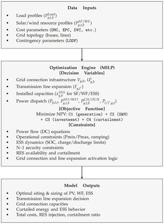
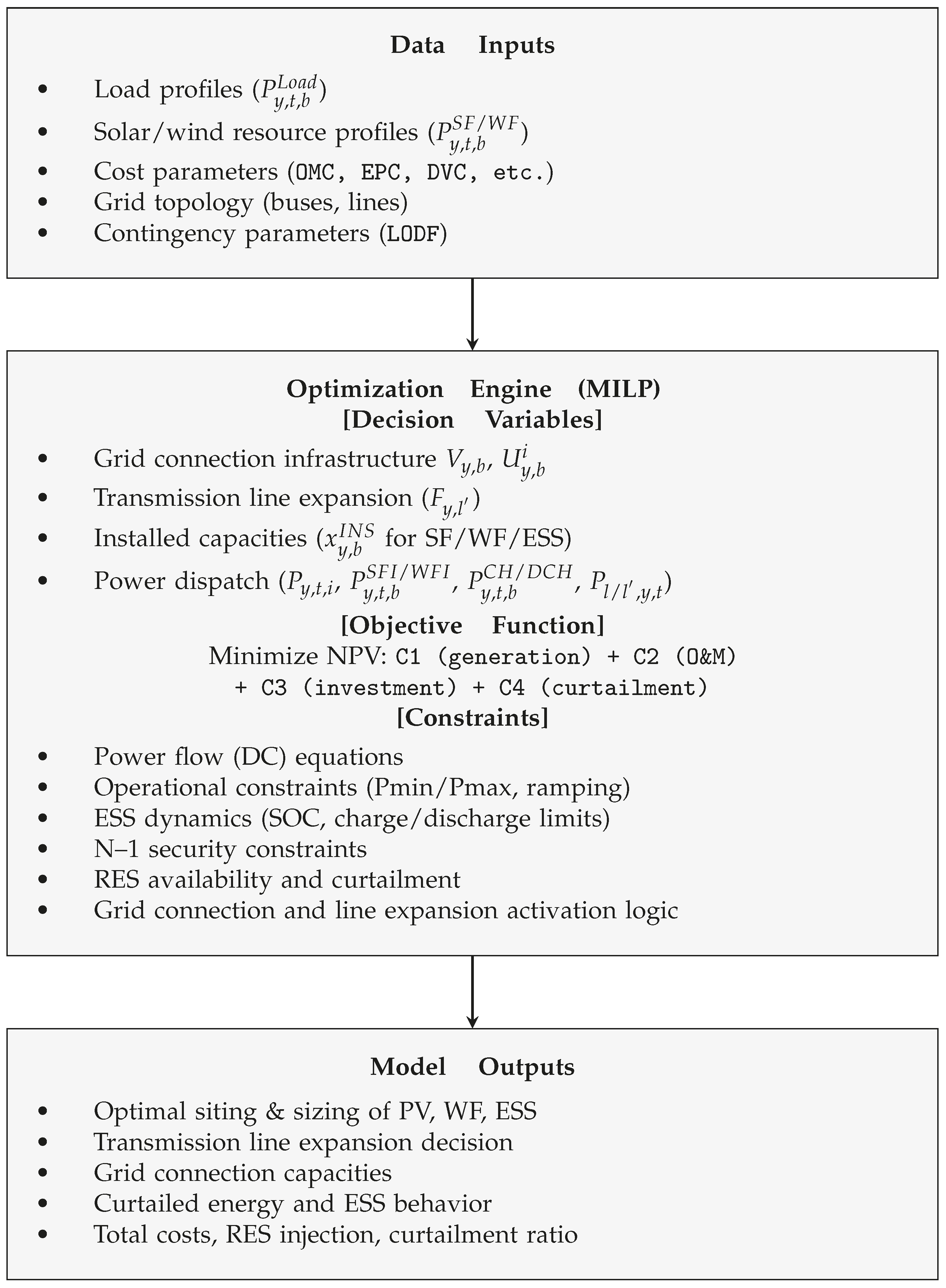
Prior to presenting the mathematical formulation of the proposed planning model, its overall structure and components are illustrated in the block diagram shown in Figure 2. This diagram outlines the key data inputs, the optimization engine including decision variables, objective function, and constraints, as well as the primary outputs of the model, providing a clear overview of its functionality and workflow.

Figure 2. Block diagram layout of the proposed model.

2.1. Objective Function

The objective function of the optimization problem to minimize the overall power generation cost, encompassing not only the fuel and operational expenditures of Thermal Units (TUs) but also the investment and operational costs linked to ESSs, WFs, SFs, and TLs. The NPV of piecewise linear costs associated with TUs is as follows:

$$C_1=\sum _{y=1}^{N_Y}{\displaystyle \frac{TU{C}_y}{{(1+IR)}^y}}$$

(1)

where

$$TU{C}_y=0.5\times 365\times \sum _{t=1}^T\sum _{i=1}^{N_G}{EC}_{y,t,i}$$

(2)

$${EC}_{y,t,i}=\sum _k{C}_{t,i}^{\left(k\right)}{P}_{y,t,i}^{\left(k\right)}$$

(3)

$$0\le P_{y,t,i}^{\left(k\right)}\le P_{y,t,i}^{\left(k\right),max}$$

(4)

$$P_{y,t,i}=\sum _k{P}_{y,t,i}^{\left(k\right)}$$

(5)

Equation (2) determines the annual cost of TUs by scaling the daily operational cost over the planning year, where the factor 0.5 accounts for the representation of the year through two characteristic days (winter and summer). Equations (3)–(5) define the piecewise linear cost function for thermal units, where Equation (3) calculates the energy cost as a sum of linear segments, Equation (4) limits each segment’s power output, and Equation (5) ensures the total power output equals the sum of all segments. The subsequent cost component under consideration pertains to the Operation and Maintenance (O&M) expenses associated with TLs, SFs, WFs, and ESSs. This category of expenditure encompasses various elements, including fixed O&M, land lease expenses, and local authority rates, which are recurrently imposed on these infrastructures on an annual basis. Additionally, certain components, such as variable O&M and balancing costs, are contingent upon the daily operational activities and energy dynamics. To ensure a comprehensive representation of the O&M cost, it is imperative to incorporate all these cost elements into the model.

$$C_2=\sum _{y=1}^{N_Y}{\displaystyle \frac{OM{C}_y}{{(1+IR)}^y}}$$

(6)

where

$$\begin{array}{cc}\hfill OM{C}_y& =0.5\times 365\times \sum _{t=1}^T\sum _{b=1}^{N_B}(OM{C}_{y,t,b}^{\mathrm{V}}+B{C}_{y,t,b})\hfill \\ \hfill & +\sum _{b=1}^{N_B}(OM{C}_{y,b}^{\mathrm{F}}+LL{E}_{y,b}+LA{R}_{y,b})\hfill \\ \hfill & +\sum _{l=1}^{N_L}({\mathrm{OMC}}_{\mathrm{TL}}^{\mathrm{F}}+{\mathrm{LLE}}_{\mathrm{TL}}){\mathrm{LL}}_l\hfill \\ \hfill & +\sum _{l^{\prime }=1}^{N_{L^{\prime }}}({\mathrm{OMC}}_{\mathrm{TL}}^{\mathrm{F}}+{\mathrm{LLE}}_{\mathrm{TL}}){\mathrm{LL}}_{l^{\prime }}\sum _{i\le y}{F}_{i,l^{\prime }}\hfill \end{array}$$

(7)

$$\begin{array}{c}\hfill \begin{array}{cc}\hfill OM{C}_{y,t,b}^{\mathrm{V}}& ={\mathrm{OMC}}_{\mathrm{SF}}^{\mathrm{V}}{P}_{y,t,b}^{SFI}+{\mathrm{OMC}}_{\mathrm{WF}}^{\mathrm{V}}{P}_{y,t,b}^{WFI}\hfill \\ \hfill & +{\mathrm{OMC}}_{\mathrm{ESS}}^{\mathrm{V}}(P_{y,t,b}^{CH}+P_{y,t,b}^{DCH})\hfill \end{array}\end{array}$$

(8a)

$$\begin{array}{cc}\hfill B{C}_{y,t,b}& ={\mathrm{BC}}_{\mathrm{SF}}{P}_{y,t,b}^{SFI}+{\mathrm{BC}}_{\mathrm{WF}}{P}_{y,t,b}^{WFI}\hfill \end{array}$$

(8b)

$$\begin{array}{c}\hfill \begin{array}{cc}\hfill & OM{C}_{y,b}^{\mathrm{F}}={\mathrm{OMC}}_{\mathrm{ESS}}^{\mathrm{F}}{\mathrm{CDR}}^{\max }{\mathrm{ESS}}_{\mathrm{unit}}\sum _{i=1}^{y}ES{S}_{i,b}^{\mathrm{INS}}\hfill \\ \hfill & +{\mathrm{OMC}}_{\mathrm{WF}}^{\mathrm{F}}{\mathrm{WF}}_{\mathrm{unit}}\sum _{i=1}^{y}W{F}_{i,b}^{\mathrm{INS}}+{\mathrm{OMC}}_{\mathrm{SF}}^{\mathrm{F}}{\mathrm{SF}}_{\mathrm{unit}}\sum _{i=1}^{y}S{F}_{i,b}^{\mathrm{INS}}\hfill \end{array}\end{array}$$

(8c)

$$\begin{array}{c}\hfill \begin{array}{cc}\hfill & LL{E}_{y,b}={\mathrm{LLE}}_{\mathrm{ESS}}{\mathrm{CDR}}^{\max }{\mathrm{ESS}}_{\mathrm{unit}}\sum _{i=1}^{y}ES{S}_{i,b}^{\mathrm{INS}}\hfill \\ \hfill & +{\mathrm{LLE}}_{\mathrm{WF}}{\mathrm{WF}}_{\mathrm{unit}}\sum _{i=1}^{y}W{F}_{i,b}^{\mathrm{INS}}+{\mathrm{LLE}}_{\mathrm{SF}}{\mathrm{SF}}_{\mathrm{unit}}\sum _{i=1}^{y}S{F}_{i,b}^{\mathrm{INS}}\hfill \end{array}\end{array}$$

(8d)

$$\begin{array}{c}\hfill \begin{array}{cc}\hfill LA{R}_{y,b}& ={\mathrm{LAR}}_{\mathrm{WF}}{\mathrm{WF}}_{\mathrm{unit}}\sum _{i=1}^{y}W{F}_{i,b}^{\mathrm{INS}}\hfill \\ \hfill & +{\mathrm{LAR}}_{\mathrm{SF}}{\mathrm{SF}}_{\mathrm{unit}}\sum _{i=1}^{y}S{F}_{i,b}^{\mathrm{INS}}\hfill \end{array}\end{array}$$

(8e)

Equation (7) calculates the annual O&M expenses, combining time-dependent variables and balancing costs (first term) with capacity-dependent fixed costs (remaining terms), where the summation over existing and potential transmission lines accounts for network expansion decisions. Equations (8a)–(8e) decompose the O&M costs into their constituent components: (8a) variable O&M costs proportional to power generation/storage operation, (8b) balancing costs for renewable energy management based on their injected energy, (8c) fixed O&M costs based on installed capacity of any asset, (8d) land lease expenses, and (8e) determines local authority regulatory costs for renewable installations. The exploration of investment costs, as outlined in Equations (9)–(12), merits discussion. Primarily, the capital expenditure linked with TLs, WFs, SFs, and ESSs consists of the spectrum of EPC (equipment and civils), development, and grid connection costs. It is noteworthy that, unlike WFs and SFs, where their EPC costs are solely contingent on the installed MW capacity, in the case of ESSs, as delineated in Equation (11d), the Storage Block Cost (SBC)—incorporating battery modules, racks, cabling, containers, and the battery management system—is reliant on the installed MWh capacity. Additionally, costs linked with Power Equipment (PE), encompassing power conversion systems and DC–DC converters, along with Control and Communication (C&C) systems, are determined by the maximum MW charge/discharge power of the ESS. In the context of HPPs, an opportunity for cost mitigation arises through the collaborative use of grid connection infrastructures. For instance, owing to the inverse correlation between solar radiation and wind speed, WFs and SFs can effectively share a smaller substation and switchyard, demonstrating a more streamlined infrastructure compared with the combined capacity of both farms. Consequently, in the proposed model, grid connections are allocated exclusively during the initial year of RES/ESS installation for a given HV bus.

$$C_3=\sum _{y=1}^{N_Y}{\displaystyle \frac{I{C}_y}{{(1+IR)}^y}}$$

(9)

where

$$\begin{array}{cc}\hfill I{C}_y& =\sum _{b=1}^{N_B}(EP{C}_{y,b}+DV{C}_{y,b}+GCo{C}_{y,b})\hfill \\ \hfill & +\sum _{l^{\prime }=1}^{N_{L^{\prime }}}({\mathrm{EPC}}^{\mathrm{TL}}+{\mathrm{DC}}^{\mathrm{TL}}){\mathrm{LL}}_{l^{\prime }}{F}_{y,l^{\prime }}\hfill \end{array}$$

(10)

$$\begin{array}{cc}\hfill EP{C}_{y,b}& =EP{C}_{y,b}^{SF}+EP{C}_{y,b}^{WF}+EP{C}_{y,b}^{ESS}\hfill \end{array}$$

(11a)

$$\begin{array}{cc}\hfill EP{C}_{y,b}^{SF}& ={\mathrm{EPC}}_{\mathrm{y}}^{\mathrm{SF}}{\mathrm{SF}}_{\mathrm{unit}}S{F}_{y,b}^{INS}\hfill \end{array}$$

(11b)

$$\begin{array}{cc}\hfill EP{C}_{y,b}^{WF}& ={\mathrm{EPC}}_{\mathrm{y}}^{\mathrm{WF}}{\mathrm{WF}}_{\mathrm{unit}}W{F}_{y,b}^{INS}\hfill \end{array}$$

(11c)

$$\begin{array}{c}\hfill \begin{array}{cc}\hfill EP{C}_{y,b}^{ESS}& ={\mathrm{SBC}}_{\mathrm{y}}^{\mathrm{ESS}}{\mathrm{ESS}}_{\mathrm{unit}}ES{S}_{y,b}^{INS}\hfill \\ \hfill & +{\mathrm{PECC}}_{\mathrm{y}}^{\mathrm{ESS}}{\mathrm{CDR}}^{\max }{\mathrm{ESS}}_{\mathrm{unit}}ES{S}_{y,b}^{INS}\hfill \end{array}\end{array}$$

(11d)

$$\begin{array}{cc}\hfill DV{C}_{y,b}& =DV{C}_{y,b}^{SF}+DV{C}_{y,b}^{WF}+DV{C}_{y,b}^{ESS}\hfill \end{array}$$

(12a)

$$\begin{array}{cc}\hfill DV{C}_{y,b}^{SF}& ={\mathrm{DC}}^{\mathrm{SF}}{\mathrm{SF}}_{\mathrm{unit}}S{F}_{y,b}^{INS}\hfill \end{array}$$

(12b)

$$\begin{array}{cc}\hfill DV{C}_{y,b}^{WF}& ={\mathrm{DC}}^{\mathrm{WF}}{\mathrm{WF}}_{\mathrm{unit}}W{F}_{y,b}^{INS}\hfill \end{array}$$

(12c)

$$\begin{array}{cc}\hfill DV{C}_{y,b}^{ESS}& ={\mathrm{DC}}^{\mathrm{ESS}}{\mathrm{ESS}}_{\mathrm{unit}}ES{S}_{y,b}^{INS}\hfill \end{array}$$

(12d)

Equation (10) aggregates the annual investment costs, including equipment and civil costs for renewable and storage technologies, development costs, grid connection costs, and TL expansion costs, where the binary variable $F_{y,l^{\prime }}$ determines the optimal timing of line $l^{\prime }$ construction. Equations (11a)–(11d) detail the equipment and civil costs: (11a) aggregates costs across technologies, (11b) and (11c) calculate costs for solar and wind farms based on installed MW capacity, while (11d) uniquely models ESS costs considering both energy capacity (MWh) through storage block cost and power capacity (MW) through power equipment and control costs. Notably, the EPC costs for RESs/ESS exhibit a consistent downward trend in the upcoming years. In the model, the EPC cost for WFs, SFs, and ESSs is reduced annually by 2%, 7%, and 5%, respectively. Equations (12) clearly represent the development cost of renewable and storage assets based on the installed capacity for each planning year.

$$\begin{array}{cc}\hfill V_{y,b}& \ge {\displaystyle \frac{1}{\mathrm{M}}}S{F}_{y,b}^{INS}-\sum _{i<y}{V}_{i,b}\hfill \end{array}$$

(13a)

$$\begin{array}{cc}\hfill V_{y,b}& \ge {\displaystyle \frac{1}{\mathrm{M}}}W{F}_{y,b}^{INS}-\sum _{i<y}{V}_{i,b}\hfill \end{array}$$

(13b)

$$\begin{array}{cc}\hfill V_{y,b}& \ge {\displaystyle \frac{1}{\mathrm{M}}}ES{S}_{y,b}^{INS}-\sum _{i<y}{V}_{i,b}\hfill \end{array}$$

(13c)

$$\begin{array}{cc}\hfill V_{y,b}& \le S{F}_{y,b}^{INS}+W{F}_{y,b}^{INS}+ES{S}_{y,b}^{INS}\hfill \end{array}$$

(13d)

$$\begin{array}{cc}\hfill V_{y,b}& \le 1-\sum _{i<y}{V}_{i,b}\hfill \end{array}$$

(13e)

Constraints (13a)–(13e) model the critical decision of grid connection infrastructure installation timing. These constraints ensure that grid connection is established only in the first year of renewable/storage deployment at each bus, preventing redundant infrastructure investments while capturing the shared connection benefits of hybrid power plants. By employing the auxiliary binary variable $V_{y,b}$ along with the big constant M, the initiation of grid connection infrastructure installation in the first year is described through Equation (13). Conditions (13a)–(13c) ensure $V_{y,b}$ is set to 1 if at least one of RES or ESS is allocated in bus b during the initial year. Additionally, constraints (13d) and (13e) guarantee that $V_{y,b}$ remains 0 in cases where there is no resource allocation or if a specific bus has already been assigned $V_{y,b}=1$ in previous years.

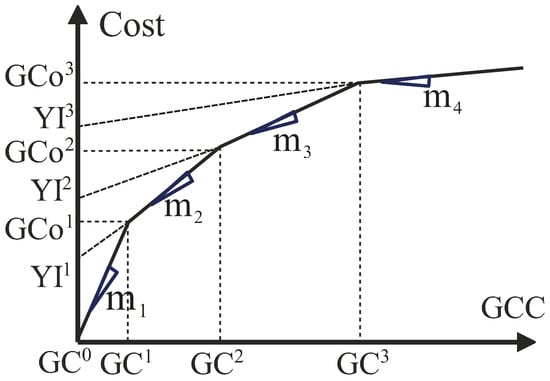
Constraints (14) set the minimum capacity required for grid connection at a designated bus. Notably, no grid connection capacity is allocated when $V_{y,b}=0$. Conversely, when $V_{y,b}=1$, the capacity allocation should be at least as substantial as the largest RES or ESS installation during that particular year. It is important to note that grid connection cost does not exhibit linear growth with increasing capacity. Therefore, to maintain linearity and accuracy in the proposed model, the connection cost is adjusted, as illustrated in Figure 3.

$$\begin{array}{cc}\hfill GC{C}_{y,b}& \le \mathrm{M}{V}_{y,b}\hfill \end{array}$$

(14a)

$$\begin{array}{cc}\hfill GC{C}_{y,b}& \ge {\mathrm{SF}}_{\mathrm{unit}}S{F}_{y,b}^{INS}-\mathrm{M}(1-V_{y,b})\hfill \end{array}$$

(14b)

$$\begin{array}{cc}\hfill GC{C}_{y,b}& \ge {\mathrm{WF}}_{\mathrm{unit}}W{F}_{y,b}^{INS}-\mathrm{M}(1-V_{y,b})\hfill \end{array}$$

(14c)

$$\begin{array}{cc}\hfill GC{C}_{y,b}& \ge {\mathrm{CDR}}^{\max }{\mathrm{ESS}}_{\mathrm{unit}}{\mathrm{ESS}}_{\mathrm{y},\mathrm{b}}^{\mathrm{INS}}-\mathrm{M}(1-{\mathrm{V}}_{\mathrm{y},\mathrm{b}})\hfill \end{array}$$

(14d)

$$\begin{array}{cc}\hfill GC{C}_{y,b}& \le {\mathrm{GC}}^{\mathrm{i}}+\mathrm{M}(1-U_{y,b}^i)\forall i\in [1,2,3,4]\hfill \end{array}$$

(15a)

$$\begin{array}{cc}\hfill GC{C}_{y,b}& \ge {\mathrm{GC}}^{\mathrm{i}-1}-\mathrm{M}(1-U_{y,b}^i)\hfill \end{array}$$

(15b)

$$\begin{array}{cc}\hfill GCo{C}_{y,b}& \ge {\mathrm{YI}}^{\mathrm{i}}+{\mathrm{m}}_{\mathrm{i}}·GC{C}_{y,b}-\mathrm{M}(1-U_{y,b}^i)\hfill \end{array}$$

(15c)

$$\begin{array}{cc}\hfill \sum _{i=1}^4{U}_{y,b}^i& =1\hfill \end{array}$$

(15d)

Figure 3. Grid connection cost for various capacities.

Constraints (15a)–(15d) implement the piecewise linear grid connection cost function depicted in Figure 3. Binary variables ($U_{y,b}^i$) activate appropriate cost segments based on connection capacity, with constraint (15c) calculating the corresponding cost and (15d) ensuring exactly one segment is active.

The ultimate cost component, denoted as curtailment costs, embodies the financial penalty imposed on the power system operator. This penalty is designed to compensate RES owners for the intentional curtailment of injecting their full available energy, often prompted by factors such as TUs’ ramp rates, grid constraints, or discrepancies between energy production and demand. Equation (17) quantifies this cost across the planning horizon.

$$C_4=\sum _{y=1}^{N_Y}{\displaystyle \frac{C{C}_y}{{(1+IR)}^y}}$$

(16)

where

$$C{C}_y=0.5\times 365\times \sum _{t=1}^T\sum _{b=1}^{N_B}c{c}_{y,t}\times (P_{y,t,b}^{WFC}+P_{y,t,b}^{SFC})$$

(17)

Finally, the overall objective function, TC, which will be minimized subject to the operational and investment constraints, is defined as follows:

$$minTC=C_1+C_2+C_3+C_4$$

(18)

2.2. Power Flow Constraints

To optimize the TC in (18), consideration of power flow constraints as well as operational and physical limits is essential. The model employs the following DC power flow for several reasons. Firstly, it avoids the complexities introduced by nonlinear AC power flow equations. Therefore, the developed planning model will be merely an MILP model with a guaranteed global optimal solution. Secondly, in the context of long-term planning, DC power flow proves to be not only valid but also pragmatic [23], given the fact that the TLs $\left(\frac{R}{X}\right)$ ratio is typically small.

$$\begin{array}{c}{\displaystyle \sum _{i\in b}}{P}_{y,t,i}+P_{y,t,b}^{DCH}+P_{y,t,b}^{SFI}+P_{y,t,b}^{WFI}\hfill \\ =P_{y,t,b}^{Load}+P_{y,t,b}^{CH}+{\displaystyle \sum _{l\in b}}{P}_{l,y,t}+{\displaystyle \sum _{l^{\prime }\in b}}{P}_{l^{\prime },y,t}\hfill \end{array}$$

(19)

$${\mathrm{RD}}_{\mathrm{i}}\le P_{y,t,i}-P_{y,t-1,i}\le {\mathrm{RU}}_{\mathrm{i}}\forall t\in [2,24]\cup [26,48]$$

(20)

$$P_{y,t,b}^{Load}=P_{y-1,t,b}^{Load}(1+L{G}_{y,b})$$

(21)

Equation (19) establishes the power balance constraint specific to a given bus, ensuring the equilibrium between generated power, load demand, and sending powers through both current ($P_l$) and potential ($P_{l^{\prime }}$) TLs. For two distinct 24-hour periods per year, representing typical winter and summer days, the ramping constraints of TUs are described in (20). Equation (21) models load growth evolution, where demand in each bus increases annually by the specified growth rate.

$$\begin{array}{cc}\hfill & P_{l,y,t}={\displaystyle \frac{1}{x_l}}({\delta }_{y,t,s}-{\delta }_{y,t,r})\forall l:\mathrm{from}\mathrm{bus}s\mathrm{to}r\hfill \end{array}$$

(22a)

$$\begin{array}{cc}\hfill & -P_{l^{\prime }}^{\mathrm{Max}}\sum _{i\le y}{F}_{i,l^{\prime }}\le P_{l^{\prime },y,t}\le P_{l^{\prime }}^{\mathrm{Max}}\sum _{i\le y}{F}_{i,l^{\prime }}\hfill \end{array}$$

(22b)

$$\begin{array}{cc}\hfill & P_{l^{\prime },y,t}\le {\displaystyle \frac{1}{x_{l^{\prime }}}}({\delta }_{y,t,s^{\prime }}-{\delta }_{y,t,r^{\prime }})+\mathrm{M}\left(1-\sum _{i\le y}{F}_{i,l^{\prime }}\right)\hfill \end{array}$$

(22c)

$$\begin{array}{cc}\hfill & P_{l^{\prime },y,t}\ge {\displaystyle \frac{1}{x_{l^{\prime }}}}({\delta }_{y,t,s^{\prime }}-{\delta }_{y,t,r^{\prime }})-\mathrm{M}\left(1-\sum _{i\le y}{F}_{i,l^{\prime }}\right)\hfill \end{array}$$

(22d)

$$\begin{array}{cc}\hfill & \sum _{y=1}^{N_y}{F}_{y,l^{\prime }}\le 1\forall l^{\prime }:\mathrm{from}\mathrm{bus}{s}^{\prime }\mathrm{to}{r}^{\prime }\hfill \end{array}$$

(22e)

$${P_i}^{\mathrm{Min}}\le P_{y,t,i}\le {P_i}^{\mathrm{Max}}$$

(23)

$$-{P_l}^{\mathrm{Max}}\le P_{l,y,t}\le {P_l}^{\mathrm{Max}}$$

(24)

Finally, Equation (22) govern the power flow of TLs. Constraints (22b)–(22d) ensure that the flow of line $l^{\prime }$ is activated if the binary variable for the line was set to 1 either in the current year or in previous years. Equation (22e) guarantees that expansion can occur only once for a given potential line. Furthermore, Equations (23) and (24) require the system’s compliance with the physical constraints of TUs and current TLs.

2.3. N − 1 Security Constraints

In the event of a transmission line/transformer failure, the flow on the affected line diminishes to zero, influencing nearby flows and potentially causing congestion. The application of the linearized approximation of DC power flow gives rise to the emergence of Linear Sensitivity Factors (LSFs). These LSFs are derived through the Jacobian Matrix and exhibit computational feasibility, even in expansive power systems. Moreover, their behavior is intricately linked to the underlying network topology. The detailed calculation of LSFs is expounded upon in Reference [24]. The Line Outage Distribution Factors (LODFs), a subset of LSFs, are specifically utilized to assess overloads when transmission circuits, such as lines or transformers, undergo failures. Its definition is as follows:

$${LODF}_{l,k}={\displaystyle \frac{\Delta f_l}{P_k}}$$

(25)

where ${\mathrm{LODF}}_{l,k,y}$ signifies the outage distribution factor when examining line l subsequent to the outage of line k. $\Delta f_l$ denotes the alteration in MW flow on line l, while $P_k$ represents the initial flow on line k before its outage occurred. By calculating the LODFs, a rapid and straightforward procedure can be established to assess all lines in the network for overloads following the possible outage of any specific line. Considering this, Equation (26) is formulated to establish line security constraints. These constraints are essential to guarantee the dependable operation of transmission line l in the event of an outage occurring on any other line k. By carefully regulating the power flow dynamics under these circumstances, the grid’s reliability and resilience are significantly enhanced.

$$-{P_l}^{\mathrm{Max}}\le P_{l,y,t}+LOD{F}_{l,k}{P}_{k,y,t}\le {P_l}^{\mathrm{Max}}$$

(26)

In this context, it is important to acknowledge that the number of $LOD{F}_{l,k}$ terms in the model reaches $N_L\times (N_L-1)$, thereby leading to a substantial proliferation of constraints, as evident in Equation (26). This proliferation poses a significant computational challenge. To mitigate this issue, a judicious approach involves excluding constraints associated with LODFs falling below a defined threshold. For instance, constraints corresponding to $LOD{F}_{l,k}<0.1$ (indicating less than 10% flow from line k goes to line l post-outage) can be omitted, strategically easing the computational burden while ensuring essential constraints remain intact.

2.4. ESS Constraints

The ESSs are subject to precise technical operational constraints as follows:

$$SO{C}_{y,t,b}\le {\mathrm{ESS}}_{\mathrm{Unit}}\sum _{i=1}^y{\mathrm{ESS}}_{i,b}^{INS}$$

(27)

$$SO{C}_{y,t,b}=SO{C}_{y,t-1,b}+P_{y,t,b}^{CH}{\eta }^{ch}-{\displaystyle \frac{P_{y,t,b}^{DCH}}{{\eta }^{dch}}}$$

(28)

$$SO{C}_{y,t,b}=\mathrm{ISOC}\times {\mathrm{ESS}}_{\mathrm{Unit}}\sum _{i=1}^{y}ES{S}_{i,b}^{INS}\forall t=0,24,48$$

(29)

$$\begin{array}{cc}\hfill P_{y,t,b}^{CH}& \le {\mathrm{CDR}}^{\max }\times {\mathrm{ESS}}_{\mathrm{Unit}}\sum _{i=1}^{y}ES{S}_{i,b}^{INS}\hfill \end{array}$$

(30a)

$$\begin{array}{cc}\hfill P_{y,t,b}^{DCH}& \le {\mathrm{CDR}}^{\max }\times {\mathrm{ESS}}_{\mathrm{Unit}}\sum _{i=1}^{y}ES{S}_{i,b}^{INS}\hfill \end{array}$$

(30b)

$$\begin{array}{cc}\hfill P_{y,t,b}^{CH}& \le \mathrm{BM}{\mathrm{I}}_{\mathrm{y},\mathrm{t},\mathrm{b}}^{\mathrm{ch}}\hfill \end{array}$$

(31a)

$$\begin{array}{cc}\hfill P_{y,t,b}^{DCH}& \le \mathrm{BM}(1-{\mathrm{I}}_{\mathrm{y},\mathrm{t},\mathrm{b}}^{\mathrm{ch}})\hfill \end{array}$$

(31b)

In Equations (27) and (28), the maximum SOC regarding the installed ESS units at each node and their dynamic changes are defined. Considering the model’s operation daily over a year, Equation (29) establishes the initial and final SOC limits for each day. Equation (30) specifies the maximum charging and discharging power of ESS. Additionally, Equation (31) utilizes a binary variable and a large positive constant to restrict simultaneous charge and discharge for a specific ESS.

2.5. RES Constraints

The available power from RESs is contingent upon factors such as wind speed in WFs and solar irradiance in SFs. To establish a realistic estimate of hourly available power, the values of wind speed and solar irradiance, derived from historical data, are employed. Equations (32)–(35) describe the available power and its correlation with curtailed and injected power into the grid. Additionally, under the model’s assumption that hybrid co-located power plants share the same grid connection infrastructures, it is crucial to restrict the injected power through the network by these sources to not surpass the apparent power of the allocated grid connection capacity at a given bus. Equations (36a) and (36b) guarantee the enforcement of this constraint.

$$P_{y,t,b}^{SF}=S{F}_{t,b}^{AP}{\mathrm{SF}}_{\mathrm{Unit}}\sum _{i=1}^{y}S{F}_{i,b}^{INS}$$

(32)

$$P_{y,t,b}^{WF}=W{F}_{t,b}^{AP}{\mathrm{WF}}_{\mathrm{Unit}}\sum _{i=1}^{y}W{F}_{i,b}^{INS}$$

(33)

$$P_{y,t,b}^{WF}=P_{y,t,b}^{WFI}+P_{y,t,b}^{WFC}$$

(34)

$$P_{y,t,b}^{SF}=P_{y,t,b}^{SFI}+P_{y,t,b}^{SFC}$$

(35)

$$\begin{array}{c}\hfill P_{y,t,b}^{SFI}+P_{y,t,b}^{WFI}-P_{y,t,b}^{CH}+P_{y,t,b}^{DCH}\le GC{C}_{y,b}\end{array}$$

(36a)

$$\begin{array}{c}\hfill P_{y,t,b}^{CH}\le GC{C}_{y,b}\end{array}$$

(36b)

3. System Parameters and Assumptions

3.1. System Parameters

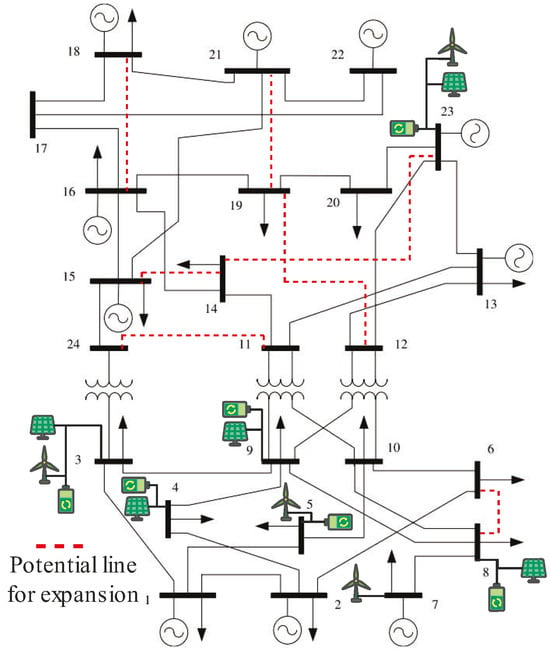
The proposed model is evaluated through simulations performed on the IEEE 24-bus test system, where the detailed network features are given in [25]. However, due to the relatively low energy cost of TUs, the energy costs in [25] are multiplied by five to tune them with the practical investment parameters. The single-line diagram of this system, including potential TLs, is depicted in Figure 4. The rationale behind selecting potential lines between pairs of buses was the higher congestion rate of the existing TLs connected to those buses. Table 1 details the set of techno-economic parameters of the proposed model.

Figure 4. Single line diagram of single area IEEE 24-bus system.

Table 1. Model parameters for the study.

	Parameter (s)	Value (s)	Parameter (s)	Value (s)
Finances	IR	4%	$C_{t,i}^{\left(k\right)}$	$5\times$ [25]
	${\mathrm{OMC}}_{SF,WF}^{\mathrm{V}}$	€2/MWh	${\mathrm{OMC}}_{ESS}^{\mathrm{V}}$	€1/MWh
	${\mathrm{BC}}_{SF,WF}$	€2/MWh	${\mathrm{OMC}}_{SF,WF}^{\mathrm{F}}$	€14.42 k/MW-y
	${\mathrm{OMC}}_{ESS}^{\mathrm{F}}$	€3 k/MW-y	${\mathrm{LLE}}_{SF,WF}$	€4.5 k/MW-y
	${\mathrm{OMC}}_{TL}^{\mathrm{F}}$	€5 k/km-y	${\mathrm{LLE}}_{TL}$	€3 k/km-y
	${\mathrm{LLE}}_{ESS}$	€500/MW-y	${\mathrm{LAR}}_{SF,WF}$	€5.14 k/MW-y
	${\mathrm{EPC}}_{y=1}^{SF}$	€450 k/MW	${\mathrm{EPC}}_{y=1}^{WF}$	€1.2 m/MW
	${\mathrm{DC}}^{ESS}$	€40 k/MWh	${\mathrm{DC}}^{SF,WF}$	€40.70 k/MW
	$c{c}_{y,t}$	€30/MWh	${\mathrm{SBC}}_{y=1}^{ESS}$	€200 k/MWh
	${\mathrm{PECC}}_{y=1}^{ESS}$	€60 k/MW	${\mathrm{EPC}}^{TL}$	€300 k/km
	${\mathrm{DC}}^{TL}$	€100 k/km	${\mathrm{GCo}}^{1,2,3}$	€2, 4.25, 6.75 m
	${\mathrm{YI}}^{1,2,3}$	€5, 17.5, 27.5k	–
Technicals	${\eta }^{ch,dch}$	90%	$L{G}_{y,b}$	5%
	${\mathrm{ESS}}_{\mathrm{unit}}$	10 MWh	$\mathrm{SF}/{\mathrm{WF}}_{\mathrm{unit}}$	20 MW
	$P_l^{\mathrm{Max}},x_l$	[25]	$P_i^{\mathrm{Min}/\mathrm{Max}}$	[25]
	${\mathrm{GC}}^{1,2,3}$	20, 50, 100 MW	$P_{y=1,t,b}^{\mathrm{Load}}$	[25]
	$\mathrm{ISOC}$	0.2	${\mathrm{CDR}}^{max}$	0.5

3.2. Renewable Energy Assumptions

The IEEE 24-bus system does not represent a power grid in any specific geographical location and was developed solely for testing and research approaches in power system studies. References [25,26,27] specify the candidate locations for installing wind and PV units based on resource availability and grid characteristics rather than geographical constraints, proposing installation options for WFs at nodes 3, 5, 7, 16, 21, and 23, as well as for SFs at nodes 3, 4, 8, 9, and 23. In practice, wind and solar atlases determine the candidate locations for installation in real-world applications. Moreover, since per-unit and DC power flow approaches are employed in the proposed model, the voltage level is normalized to 1 p.u. for all nodes, making geographical zoning and multiple voltage level considerations unnecessary for the proposed model.

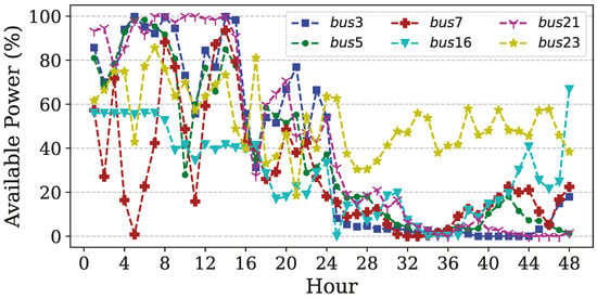
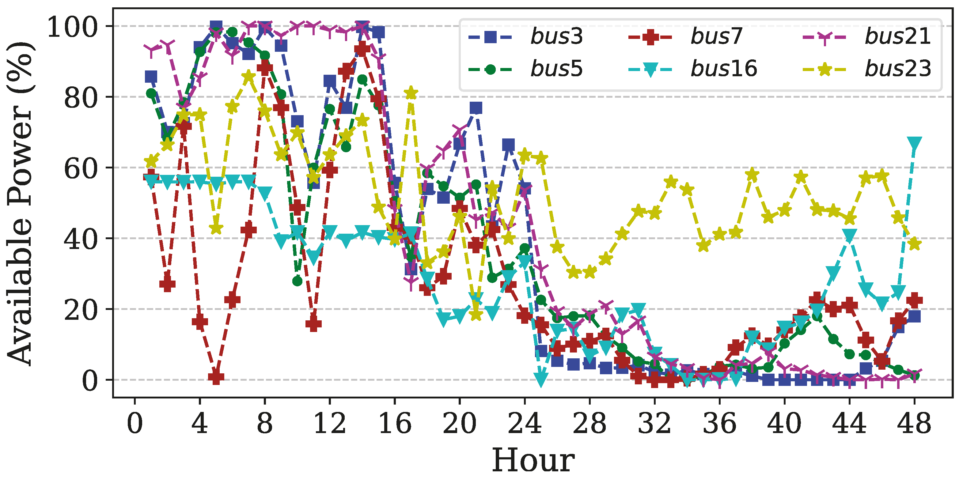
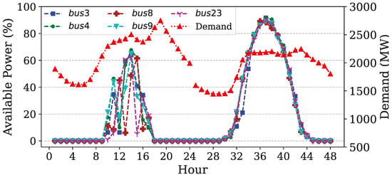
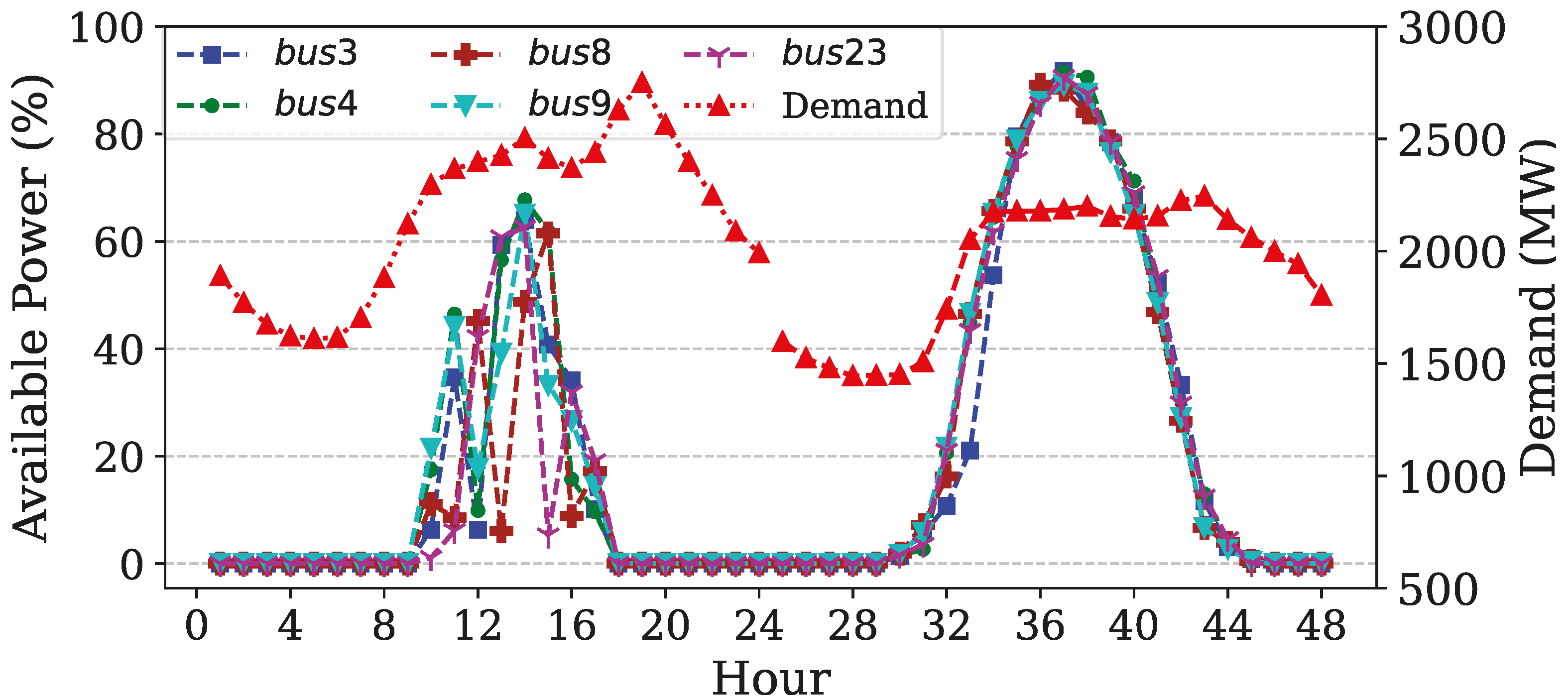
The estimated hourly power available for prospective WFs and SFs can be approached using three primary methods. The first method utilizes hourly power availability data for the entire year, leading to an extremely large number of decision variables, on the order of $365\times T\times N_Y\times V_t$, where $V_t$ denotes the number of variables indexed by time t. This scale renders the resulting optimization model computationally intractable. The second method employs hourly mean values averaged across the year, substantially reducing the computational burden while preserving the total annual available energy. However, this simplification results in overly smoothed power profiles that fail to capture the intrinsic intermittency of RESs, causing them to behave similarly to conventional thermal generators. As a result, this method neglects the operational benefits of ESSs and the energy curtailment concept. The third approach, adopted in this study, selects two representative 24-h days per year from historical weather data from a European country: one winter day with high wind availability and one summer day with high solar irradiance. These samples are chosen such that the average of their combined available power closely approximates the annual average derived from hourly data. This method effectively retains the diurnal and seasonal variability of RES while accurately representing the annual Expected Available Power (EAP) profiles for wind and solar generation at prospective integration nodes. Specifically, Figure 5 and Figure 6 illustrate the EAP profiles derived from the first year’s data samples. Similarly, independent RES profiles are considered for any RES location in each remaining year within the planning horizon. A comparison between the EAP of WFs and SFs during winter and summer demonstrates the inverse correlation between these two sources, revealing the benefit of HPPs. Additionally, there is no prescribed limitation on the location of ESSs.

Figure 5. Hourly WFs available power by season in 1st year.

Figure 6. Hourly demand and SFs available power by season in 1st year.

4. Model Evaluation

This section assesses the proposed HPP-based planning model in comparison with a conventional renewable energy and storage system planning framework, using the IEEE 24-bus test system and the parameters defined in Section 3. The proposed model is implemented in the Python programming language (version 3.12.5) using the Pyomo [28] optimization modeling library, with the MILP formulation solved using the IBM CPLEX solver via Pyomo’s interface. Python handles all model stages, including (1) data preprocessing of network parameters and techno-economic data, (2) model formulation with symbolic variables and constraints in Pyomo, (3) solver execution through CPLEX, and (4) post-processing and verification using Matplotlib (version 3.9.2) and Pandas (version 2.2.3) packages for results validation and visualization. In this section, two case studies are conducted: Case Study 1 implements the full HPP model formulated as an MILP problem, incorporating Equations (1>)–(36). Case Study 2 applies the same parameters and constraints but omits Equations (13a)–(13e), (14a)–(14d), and (36a) and (36b), along with the binary variable $V_{y,b}$. Instead, it introduces Equation (37) to set the grid connection capacity:

$${\mathrm{GCC}}_{y,b}\ge {\mathrm{CDR}}^{max}\times {\mathrm{ESS}}_{\mathrm{unit}}\times {\mathrm{ESS}}_{y,b}^{\mathrm{INS}}+{\mathrm{WF}}_{\mathrm{unit}}\times {\mathrm{WF}}_{y,b}^{\mathrm{INS}}+{\mathrm{SF}}_{\mathrm{unit}}\times {\mathrm{SF}}_{y,b}^{\mathrm{INS}}$$

(37)

4.1. Case Study 1: HPP Planning

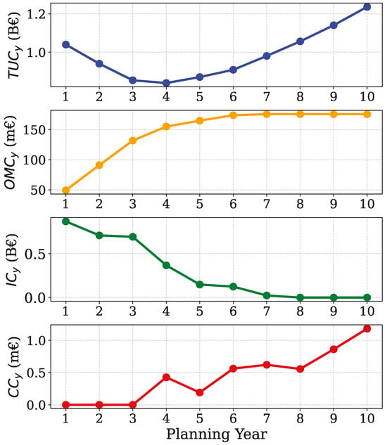
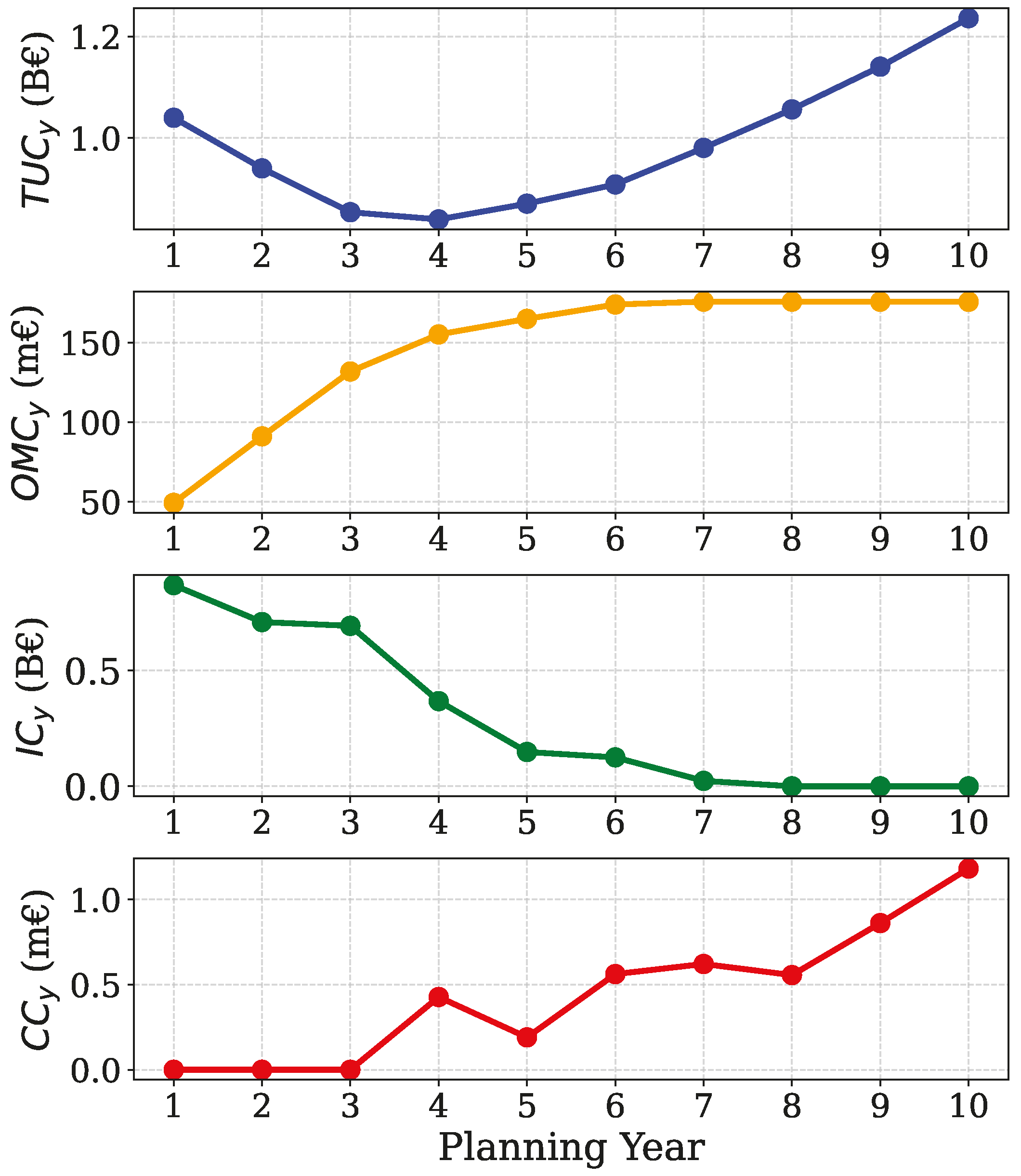
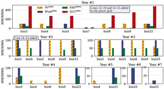
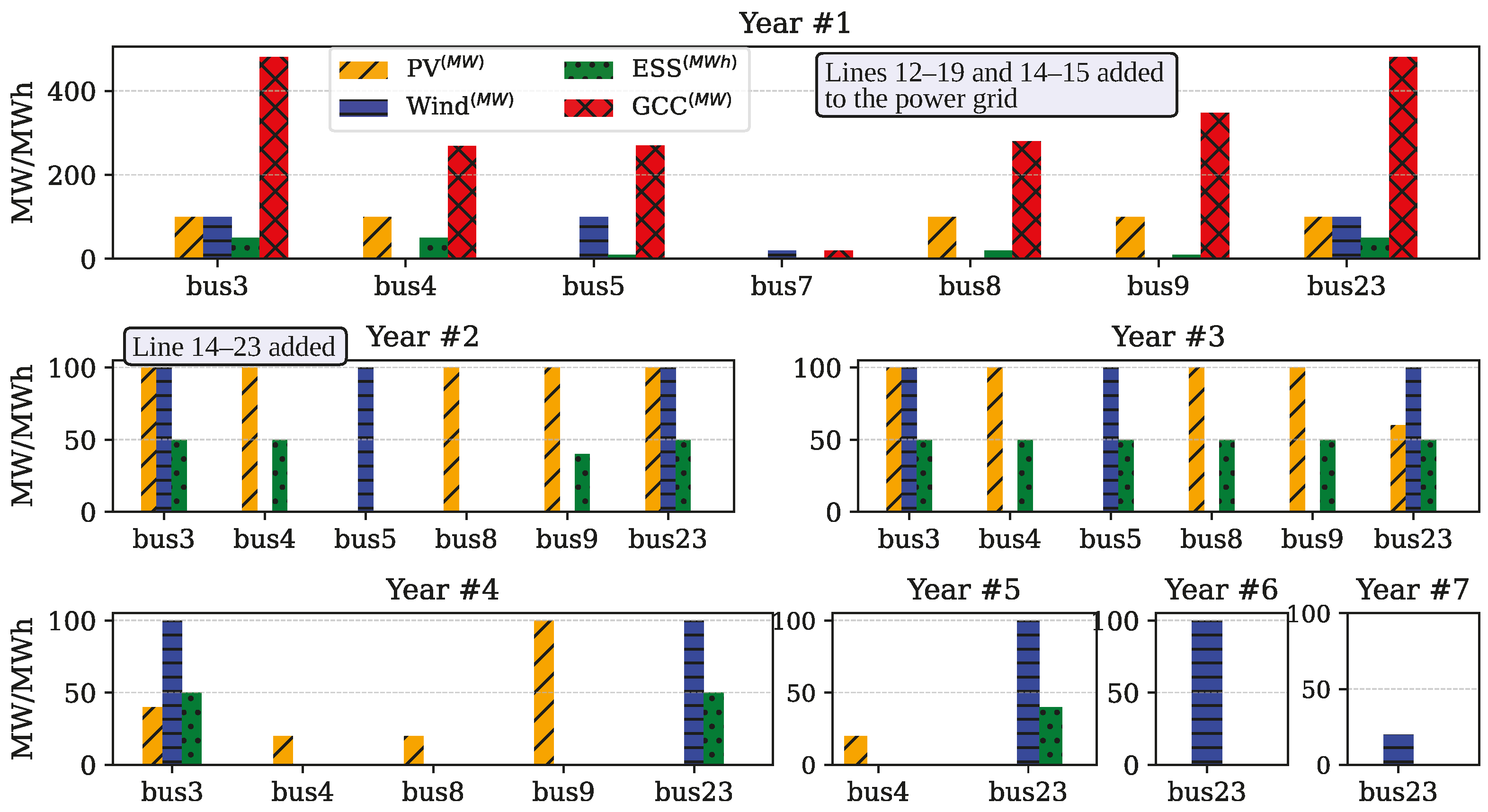
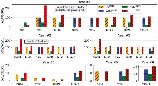
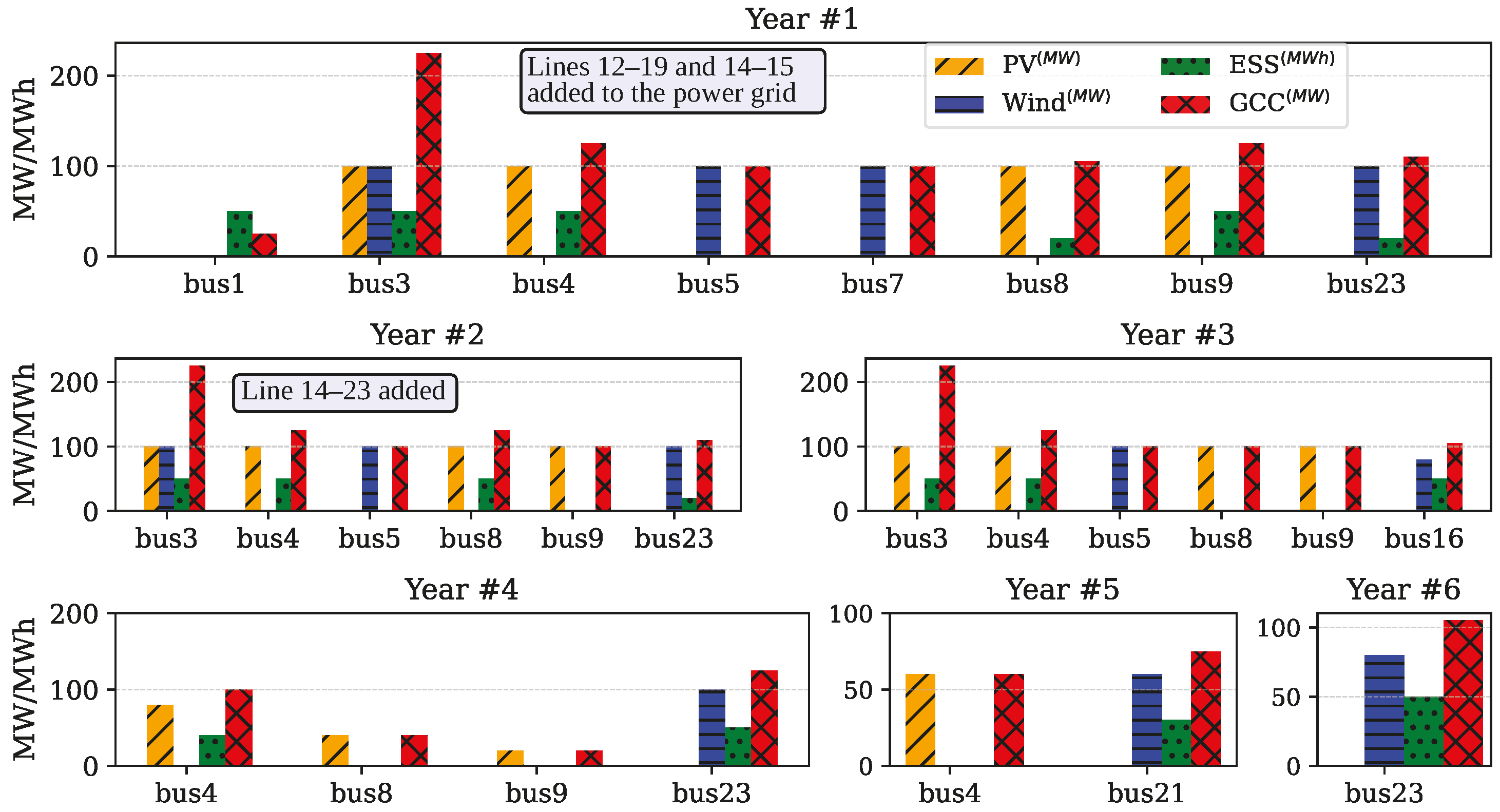
This subsection presents the planning results obtained from the proposed HPP model. Table 2 summarizes the NPV of the cost components, while Figure 7 illustrates the corresponding cash flows, providing a clear financial overview. The cash flow analysis shows a steady reduction in the TUs’ operational cost ($C_1$) during the first half of the planning horizon, driven by early investments in cost-effective RES installations. In the later years, however, load growth combined with reduced investment levels reverses this trend. Curtailment costs ($C_4$) remain zero for the first three years due to timely ESS and TL expansions but begin to rise from year 6 onward as higher RES penetration and load growth exacerbate grid constraints. Figure 8 depicts the temporal allocation of PV, WF, ESS, GCC, and TL installations. Early years are characterized by substantial RES deployment to maximize lifetime energy yield, and the integration of multiple RES units into HPP configurations is evident. For example, at bus 3, the model allocates 400 MW of WF, 340 MW of PV, and 200 MWh (100 MW) of ESS, supported by only 481 MW of GCC over the planning horizon.

Table 2. NPV of different cost components for HPP model.

${\mathit{C}}_1$	${\mathit{C}}_2$	${\mathit{C}}_3$	${\mathit{C}}_4$	$\mathbf{TC}$
€8.351B	€1.105B	€2.768B	€3.380m	€12.23B

Figure 7. Cash flows of HPP model’s cost components over the planning horizon.

Figure 8. Planning decisions by the proposed HPP model.

4.2. Case Study 2: Independent Plant Planning

The independent plant model yields distinct investment strategies driven by separate grid connection requirements for each technology. Table 3 details the financial breakdown, revealing conservative resource deployment patterns influenced by individual connection costs. As illustrated in Figure 9, the allocation timeline spans six years, and like the HPP model, the optimization triggers grid reinforcement through the addition of transmission lines 12–19, 14–15, and 14–23 to accommodate the increased generation capacity.

Table 3. NPV of different cost components for independent model.

${\mathit{C}}_1$	${\mathit{C}}_2$	${\mathit{C}}_3$	${\mathit{C}}_4$	$\mathbf{TC}$
€9.406B	€0.902B	€2.301B	€2.910m	€12.61B

Figure 9. Planning decisions by the independent model.

4.3. Hybrid vs. Independent Model Performance

Table 4 compares the proposed HPP-based planning approach with a conventional independent RES and storage model using separate grid connections. Note that the solver and its corresponding settings and model parameters were the same. The results show that the HPP model achieves a lower total cost ($TC$) and significantly reduces grid connection costs ($GCoC$), despite integrating 480 MW more renewable capacity. This improvement stems from the coordinated design, which requires only a single connection permit and land allocation per node. While emissions are not explicitly modeled, the higher renewable penetration in the HPP case implicitly indicates reduced thermal unit emissions. Overall, the results confirm the HPP model’s superior efficiency, economic viability, and potential to enhance large-scale RES integration.

Table 4. Comparative performance of HPP vs. independent plant models.

Variable	HPP Model	Independent Model
$TC$	€12.23B	€12.61B
RESs allocation	3000 (MW)	2520 (MW)
ESSs allocation	820 (MWh)/410 (MW)	730 (MWh)/365 (MW)
Total $GCoC$	€103.69 m	€214.88 m
Calculation time	580 s	232 s
Iterations (nodes)	28,510	9221

4.4. Sensitivity Analyses

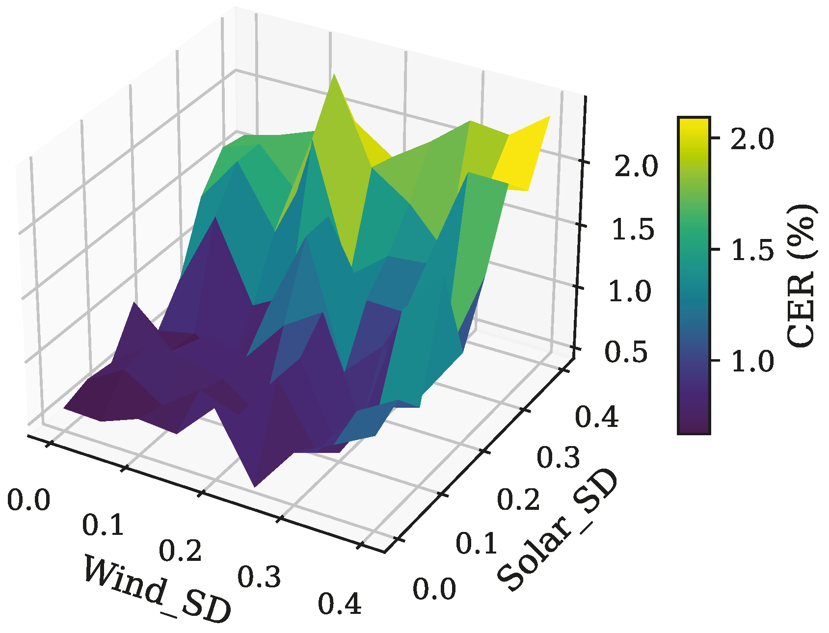
This section examines the sensitivity of the Curtailed Energy Ratio (CER) to the intermittent nature of RESs, particularly focusing on the stochastic behaviors of wind speed and solar irradiance. The CER is defined as

$$CER\%=\sum _{y=1}^{N_Y}\sum _{b=1}^{N_B}\sum _{t=1}^T{\displaystyle \frac{P_{y,t,b}^{WFC}+P_{y,t,b}^{SFC}}{P_{y,t,b}^{WF}+P_{y,t,b}^{SF}}}\times 100$$

(38)

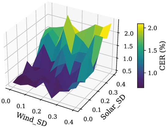
This analysis is conducted by assuming that the TLs, WFs, SFs, and ESSs are installed during the planning horizon as depicted in Figure 8. So, by excluding the investment variables, the model is solved for randomly generated EAPs derived from Normal Probability Distribution Functions (PDFs) with varying Standard Deviations (SDs). As illustrated in Figure 10, the results reveal a clear trend: higher uncertainty in RESs leads to increased CER values. This finding highlights the energy curtailment posed by variability in RESs’ energy output.

Figure 10. CER vs. uncertainty in EAPs from RESs.

Also, one of the pivotal factors influencing the allocation of ESS and the curtailed energy of RES is the curtailment cost. To assess the impact of this parameter, the proposed model is solved for various curtailment cost levels. Analysis of the results given in Table 5 reveals that as the curtailment cost escalates, there is a consistent reduction in curtailed energy. This trend is facilitated by either increasing the installed capacity of ESSs or reducing the deployed RESs capacity.

Table 5. Impact of curtailment cost on RES/ESS allocation and curtailed energy.

Curtailment Cost (€/MWh)	Total RESs Allocation (MW)	Total ESSs Allocation (MWh)	CER (%)
5	3140	760	1.29
15	3100	780	0.99
30	3000	820	0.22
50	2960	800	0.15
80	2980	830	0.06

Table 6 illustrates the impact of N − 1 security constraints on the outcomes of the proposed planning model. In the presence of security constraints, the ESS allocation is higher at 820 (MWh) compared with 760 (MWh) without constraints. Conversely, the injected energy by RESs decreased from 68.26 (TWh) in the case of excluding the security constraints to 67.46 (TWh) in the case of considering the N − 1 security criterion. Moreover, the observed increase in RESs curtailed energy from 120.0 (GWh) to 148.8 (GWh) when security constraints are imposed, underscoring the incurred cost of maintaining system reliability in the case of N − 1 contingencies.

Table 6. Comparative analysis of the model results with and without line security constraints.

Variable	Security Constrained	Without Security Constraints
$TC$	€12.23B	€11.49B
RESs allocation	3000 (MW)	3040 (MW)
ESSs allocation	820 (MWh)/410 (MW)	760 (MWh)/380 (MW)
RESs injected energy	67.46 (TWh)	68.26 (TWh)
RESs curtailed energy	148.8 (GWh)	120.0 (GWh)

Table 7 presents a sensitivity analysis of the EPC cost reduction rates for PV, wind, and ESS systems, considering three different scenarios: the base case, optimistic reduction, and pessimistic reduction. In the base case, the annual cost reductions are assumed to be 7% for PV, 2% for wind, and 5% for ESS. The optimistic case assumes more significant cost reductions, with 14% for PV, 4% for wind, and 10% for ESS, resulting in slightly higher total installations and deferred investments over the planning horizon. In contrast, the pessimistic case assumes no cost reduction (0% for all), leading to more front-loaded investments and slightly lower overall system capacities. The table also shows how these different cost reduction rates influence the total RES and ESS capacities, as well as the first and final year allocations for both types of installations. The last planning year varies for each case, reflecting how the cost reductions impact the timing and distribution of investments.

Table 7. Sensitivity analysis of EPC cost reduction rates on long-term planning outcomes.

	Base Case	Optimistic Case	Pessimistic Case
Final planning year	7	8	6
Total RES capacity (MW)	3000	3120	2940
Total ESS capacity (MWh)	820	870	780
RES in 1st year (MW)	820	780	820
ESS in 1st year (MWh)	180	150	200
RES in final year (MW)	20	80	80
ESS in final year (MWh)	0	30	0

5. Discussion

The proposed HPP planning framework achieves significant cost savings, higher renewable penetration, and reduced grid connection costs compared with the conventional independent plant model. Results from the IEEE 24-bus case studies highlight the benefits of early renewable installation, co-location of multiple RES with ESS, and optimized grid connection capacity, which together enhance flexibility, reduce curtailment, and improve long-term operational efficiency. These findings confirm the HPP model’s potential to support large-scale renewable integration while maintaining system reliability. While the IEEE 24-bus system is used for clarity and reproducibility, the proposed MILP-based model is fully scalable to larger systems due to its linear structure. Although MILP problems are NP-hard in general, the number of variables and constraints in this formulation grows approximately linearly with the number of buses, time periods, and planning years, making it tractable for modern solvers such as CPLEX. Scalability is further enhanced by avoiding nonlinearities (via DC power flow and piecewise linear costs), restricting large constants to small ranges, using representative time periods (48 h per year), and applying LODF thresholds to reduce model size. These features enable efficient, globally optimal solutions even for large-scale grids.

6. Conclusions

This paper introduces a long-term capacity planning optimization model for hybrid RESs and ESSs, jointly considering transmission line expansion. The proposed MILP framework aims to minimize total costs while ensuring system reliability through N − 1 line security constraints. A distinguishing feature of the model is the explicit representation of HPPs with shared grid connection capacities, enabling coordinated siting and sizing decisions for PV, wind, and ESS units. The results highlight the pivotal role of ESS in enabling high levels of RES integration, mitigating variability in operational costs, and reducing energy curtailment. Key findings include the following:

• Cost savings are achieved by allocating a reduced amount of GCC through the utilization of shared infrastructure among RESs and ESSs.
• Integration of ESS into HPPs offers two benefits: alleviating the variability of operation costs imposed by uncertainty in EAPs of RESs and mitigating the undesirable curtailed energy of RESs.
• Curtailment cost is a key factor influencing ESS allocation and RES energy curtailment. The results show that as curtailment costs rise, curtailed energy decreases, facilitated by either increasing ESS capacity or reducing RES capacity.
• With N − 1 security constraints, ESS allocation increases, and injected energy by RESs decreases, while the curtailed energy by RES rises, which highlights the cost of maintaining system reliability.
• The planning model, by incorporating the HPPs, shows lower overall costs and greater renewable integration, requiring only a single permission and land allocation per node for grid connection.

While the proposed framework effectively integrates HPPs into long-term capacity planning with N − 1 security constraints, several aspects remain beyond its current scope. Further research could explore:

• Incorporation of more granular temporal resolution and extreme-event modeling: The present study uses representative days to manage computational complexity. Future work can incorporate higher-resolution time series (including extreme weather events) to better capture short-term operational dynamics and resilience.
• Explicit modeling of market and regulatory mechanisms: The current framework optimizes purely from a techno-economic perspective. Including emissions trading schemes, capacity markets, and ancillary service markets would provide a more comprehensive assessment of investment strategies.
• Integration of emerging flexibility technologies: Technologies such as seasonal energy storage, power-to-X (e.g., hydrogen production), and advanced demand response could further enhance system flexibility and renewable absorption.
• Detailed reliability and resilience analysis: While N − 1 security is included, additional reliability criteria (e.g., N − 2 contingencies, probabilistic outage modeling, cyber-physical security) could be considered for more robust planning in critical infrastructure scenarios.

References

- Singh, R.; Bansal, R.C. Optimization of an autonomous hybrid renewable energy system using reformed electric system cascade analysis. IEEE Trans. Ind. Inform. 2019, 15, 399–409. [Google Scholar] [CrossRef] [Scilit]
- Reveles-Miranda, M.; Ramirez-Rivera, V.; Pacheco-Catalán, D. Hybrid energy storage: Features, applications, and ancillary benefits. Renew. Sustain. Energy Rev. 2024, 192, 114196. [Google Scholar] [CrossRef] [Scilit]
- Han, S.; Kim, H.J.; Lee, D. A Long-Term Evaluation on Transmission Line Expansion Planning with Multistage Stochastic Programming. Energies 2020, 13, 1899. [Google Scholar] [CrossRef] [Scilit]
- Mohseni-Bonab, S.M.; Kamwa, I.; Moeini, A.; Rabiee, A. Voltage Security Constrained Stochastic Programming Model for Day-Ahead BESS Schedule in Co-Optimization of T & D Systems. IEEE Trans. Sustain. Energy 2020, 11, 391–404. [Google Scholar] [CrossRef] [Scilit]
- Hooshmand, E.; Rabiee, A. Robust model for optimal allocation of renewable energy sources, energy storage systems and demand response in distribution systems via information gap decision theory. IET Gener. Transm. Distrib. 2019, 13, 511–520. [Google Scholar] [CrossRef] [Scilit]
- Aghamohamadi, M.; Mahmoudi, A.; Haque, M.H. Adaptive robust recourse-based bidding strategy and capacity allocation of PV-WT-BES owning prosumers under uncertainties. IEEE Trans. Ind. Appl. 2021, 57, 4170–4186. [Google Scholar] [CrossRef] [Scilit]
- Li, J.; Wang, C.; Wang, H. Attentive Convolutional Deep Reinforcement Learning for Optimizing Solar-Storage Systems in Real-Time Electricity Markets. IEEE Trans. Ind. Inform. 2024, 20, 7205–7215. [Google Scholar] [CrossRef] [Scilit]
- Yazdani, H.; Doostizadeh, M.; Aminifar, F. Forecast-aided power and flexibility trading of prosumers in peer to peer markets. IET Renew. Power Gener. 2023, 17, 920–934. [Google Scholar] [CrossRef] [Scilit]
- Mi, Y.; Tao, B.; Fu, Y.; Su, X.J.; Wang, P. A Game Bidding Model of Electricity and Hydrogen Sharing System Considering Uncertainty. IEEE Trans. Smart Grid 2024, 15, 2751–2761. [Google Scholar] [CrossRef] [Scilit]
- Murphy, C.A.; Schleifer, A.; Eurek, K. A taxonomy of systems that combine utility-scale renewable energy and energy storage technologies. Renew. Sustain. Energy Rev. 2021, 139, 110711. [Google Scholar] [CrossRef] [Scilit]
- Bade, S.O.; Meenakshisundaram, A.; Tomomewo, O.S. Current Status, Sizing Methodologies, Optimization Techniques, and Energy Management and Control Strategies for Co-Located Utility-Scale Wind–Solar-Based Hybrid Power Plants: A Review. Eng 2024, 5, 677–719. [Google Scholar] [CrossRef] [Scilit]
- Habbou, H.; Leon, J.P.M.; Das, K. Profitability of hybrid power plants in European markets. J. Phys. Conf. Ser. 2023, 2507, 012009. [Google Scholar] [CrossRef] [Scilit]
- Stanley, A.P.; King, J. Optimizing the physical design and layout of a resilient wind, solar, and storage hybrid power plant. Appl. Energy 2022, 317, 119139. [Google Scholar] [CrossRef] [Scilit]
- Lindberg, O.; Arnqvist, J.; Munkhammar, J.; Lingfors, D. Review on power-production modeling of hybrid wind and PV power parks. J. Renew. Sustain. Energy 2021, 13, 042702. [Google Scholar] [CrossRef] [Scilit]
- Deng, Y.; Fang, X.; Gao, N.; Tan, J. Multi-Timescale Optimal Operation Framework for Integrated Economic and Reliability Analysis of Hybrid Power Plants. In Proceedings of the 2024 IEEE Power & Energy Society General Meeting (PESGM), Seattle, WA, USA, 21–25 July 2024; pp. 1–5. [Google Scholar] [CrossRef] [Scilit]
- Atherton, J.; Akroyd, J.; Farazi, F.; Mosbach, S.; Lim, M.Q.; Kraft, M. British wind farm ESS attachments: Curtailment reduction vs. price arbitrage. Energy Environ. Sci. 2023, 16, 4020–4040. [Google Scholar] [CrossRef] [Scilit]
- Panda, D.K.; Das, S. Economic operational analytics for energy storage placement at different grid locations and contingency scenarios with stochastic wind profiles. Renew. Sustain. Energy Rev. 2021, 137, 110474. [Google Scholar] [CrossRef] [Scilit]
- Li, J.; Liu, P.; Li, Z. Optimal design of a hybrid renewable energy system with grid connection and comparison of techno-economic performances with an off-grid system: A case study of West China. Comput. Chem. Eng. 2022, 159, 107657. [Google Scholar] [CrossRef] [Scilit]
- Suresh, V.; Muralidhar, M.; Kiranmayi, R. Modelling and optimization of an off-grid hybrid renewable energy system for electrification in a rural areas. Energy Rep. 2020, 6, 594–604. [Google Scholar] [CrossRef] [Scilit]
- Cai, W.; Li, X.; Maleki, A.; Pourfayaz, F.; Rosen, M.A.; Nazari, M.A.; Bui, D.T. Optimal sizing and location based on economic parameters for an off-grid application of a hybrid system with photovoltaic, battery and diesel technology. Energy 2020, 201, 117480. [Google Scholar] [CrossRef] [Scilit]
- Hlal, M.I.; Ramachandaramurthy, V.K.; Sarhan, A.; Pouryekta, A.; Subramaniam, U. Optimum battery depth of discharge for off-grid solar PV/battery system. J. Energy Storage 2019, 26, 100999. [Google Scholar] [CrossRef] [Scilit]
- Luta, D.N.; Raji, A.K. Decision-making between a grid extension and a rural renewable off-grid system with hydrogen generation. Int. J. Hydrogen Energy 2018, 43, 9535–9548. [Google Scholar] [CrossRef] [Scilit]
- Ploussard, Q.; Olmos, L.; Ramos, A. A search space reduction method for transmission expansion planning using an iterative refinement of the DC load flow model. IEEE Trans. Power Syst. 2019, 35, 152–162. [Google Scholar] [CrossRef] [Scilit]
- Wood, A.J.; Wollenberg, B.F.; Sheblé, G.B. Power Generation, Operation, and Control; John Wiley & Sons: Hoboken, NJ, USA, 2013. [Google Scholar]
- Ordoudis, C.; Pinson, P.; Morales, J.M.; Zugno, M. An Updated Version of the IEEE RTS 24-Bus System for Electricity Market and Power System Operation Studies; Technical University of Denmark: Lyngby, Denmark, 2016; Volume 13. [Google Scholar]
- Zugno, M.; Conejo, A.J. A robust optimization approach to energy and reserve dispatch in electricity markets. Eur. J. Oper. Res. 2015, 247, 659–671. [Google Scholar] [CrossRef] [Scilit]
- Tawfiq, A.A.E.; El-Raouf, M.O.A.; Mosaad, M.I.; Gawad, A.F.A.; Farahat, M.A.E. Optimal reliability study of grid-connected PV systems using evolutionary computing techniques. IEEE Access 2021, 9, 42125–42139. [Google Scholar] [CrossRef] [Scilit]
- Hart, W.E.; Watson, J.P.; Woodruff, D.L. Pyomo: Modeling and solving mathematical programs in Python. Math. Program. Comput. 2011, 3, 219–260. [Google Scholar] [CrossRef] [Scilit]
Disclaimer/Publisher’s Note: The statements, opinions and data contained in all publications are solely those of the individual author(s) and contributor(s) and not of MDPI and/or the editor(s). MDPI and/or the editor(s) disclaim responsibility for any injury to people or property resulting from any ideas, methods, instructions or products referred to in the content. |
© 2025 by the authors. Licensee MDPI, Basel, Switzerland. This article is an open access article distributed under the terms and conditions of the Creative Commons Attribution (CC BY) license (https://creativecommons.org/licenses/by/4.0/).