Structure Optimization of Ensemble Learning Methods and Seasonal Decomposition Approaches to Energy Price Forecasting in Latin America: A Case Study about Mexico

Abstract

The energy price influences the interest in investment, which leads to economic development. An estimate of the future energy price can support the planning of industrial expansions and provide information to avoid times of recession. This paper evaluates adaptive boosting (AdaBoost), bootstrap aggregation (bagging), gradient boosting, histogram-based gradient boosting, and random forest ensemble learning models for forecasting energy prices in Latin America, especially in a case study about Mexico. Seasonal decomposition of the time series is used to reduce unrepresentative variations. The Optuna using tree-structured Parzen estimator, optimizes the structure of the ensembles through a voter by combining several ensemble frameworks; thus an optimized hybrid ensemble learning method is proposed. The results show that the proposed method has a higher performance than the state-of-the-art ensemble learning methods, with a mean squared error of 3.37 × 10${}^{-9}$ in the testing phase.

1. Introduction

Energy supply is an important factor in creating jobs and promoting economic development. Energy is needed to generate the power to operate production and service centers. The quality and reliability of energy supplies are also essential to economic and social development [1]. This is the reason the Mexican government has been investing in infrastructure to ensure that the energy supply in the country has quality, reliable, and achieves the viability needed for sustainable development [2].

Compared to other countries, Mexico has relatively low electricity prices since it has a lower cost for power generation, encouraging investment in the country’s industrial development [3]. Furthermore, access to electricity and the use of energy has generated significant social development in Mexico. Electricity has improved people’s quality of life, making them more productive and connected. Energy has allowed for increased productivity in many areas, which has contributed to the country’s economic growth [4].

The variations in the price of energy directly impact the lives of the population and the projection of the country’s development. A lower energy price is an alternative to reducing the fixed cost of production of goods and consumption, so having an estimate of future energy prices can help in the planning of industrial expansion. Another important aspect related to the price of energy is that its lower price improves people’s quality of life, resulting in greater access to electricity, and the forecast can be used to assess future scenarios and develop public policies with the intent of social development. Based on these two aspects, evaluating the price variation over time and making a prediction can assist in decision-making regarding the development of policies that reduce the price of energy to encourage the country’s development [5].

In time series, the variation that occurs in the measurements due to the recording interval, besides the variation due to different days of the week, may not give an accurate indication of the variation trend [6]. For this reason, the data need to be preprocessed to mitigate the impact of these unrepresentative variations on the trend. The ensemble learning methods are widely employed since they typically require a lower computational effort than deep learning-based techniques while maintaining their performance [7]. This paper uses seasonal decomposition using moving averages (SDMA) to reduce signal variation and ensemble learning approaches to achieve future energy price forecasting.

The main contributions of this paper are:

• The reduction of the signal variation is achieved by using the seasonal decomposition using moving averages. This technique can be used for denoising (noise reduction) in chaotic time series.
• A comparison of the adaptive boosting (AdaBoost), bootstrap aggregation (Bagging), Gradient Boosting, Histogram-Based Gradient Boosting, and Random Forest ensemble learning models are evaluated.
• An optimized ensemble learning method is presented, combining multiple ensembles and determining the best model structure using a voter selected through Optuna.

The remainder of this paper is organized as follows: Section 2 presents works related to time series forecasting and energy. In Section 3, the proposed method is explained, and the dataset is presented. In Section 4, the results are evaluated and, discussed, and in Section 5 a conclusion and final comments are presented.

2. Related Works

Three machine learning models, including extreme learning machine, gradient boosting machine, and support vector regression, as well as the Gaussian process, were applied by Ribeiro et al. [8] in forecasting one, two, and three-month ahead electricity prices in the Brazilian market. Exogenous variables were considered in the input of the models, and decomposition was used. The proposed model improved the accuracy and stability of the forecasts.

Four different approaches to forecasting the spot price of electricity in Germany for different horizons, 1, 7, and 30 days ahead, were compared by Lehna et al. [9]. In addition to the prominent seasonal auto-regressive integrated moving average model and long-term memory (LSTM) models, an LSTM convolutional neural network and a two-stage multivariate vector auto-regressive approach were used as hybrid models. External influences such as consumer load, fuel prices, carbon dioxide emission, average solar radiation, and wind speed were added.

Convolutional networks are increasingly being explored, showing promise in many applications [10], including time series [11]. Shao et al. [12] proposed a hybrid model integrating deep learning model, feature extraction, and feature selection method to forecast 1-h and 24-h ahead electricity prices for Pennsylvania, New Jersey, and Maryland; however, today includes other territories and New South Wale electricity markets from the United States of America. The results were promising, outperforming previous alternatives.

Baule and Naumann [13] used and analyzed five measures for electricity price fluctuations in the German market, and identified key factors of price fluctuations, among them wind, traded volume, auction price, and volume-weighted intraday price. They noted that trade-related variables are important in predicting price fluctuations.

Zang et al. [14] used price data from Australian and Spanish electricity markets for empirical analysis, applying joint empirical modal decomposition on the residual term after variational modal decomposition to improve the prediction accuracy of the extreme learning machine (ELM) model optimized differential evolution (DE) algorithm, introducing the DE-ELM meta-learner to optimize the reconstruction weights of the prediction components, and building an efficient and new hybrid model.

A data-driven deep learning network was used by Yang et al. [15] to capture the temporal distribution of electricity prices in real-time. A module based on GoogLeNet was developed to capture the high frequencies of these data and added time series summary statistics to improve the prediction of volatile price spikes. The model was validated on the prices of many generators in the New York Independent System Operator, improving performance compared to the model used in practice.

The operation data of Denmark’s DK1 region in the Nordic electricity market were adopted for electricity price forecasting, including wind power generation in the study of Wang et al. [16], showing that the hybrid model composed of Random Forest, best Mahalanobis distance, and bi-directional short-term memory significantly improved the forecasting performance, with better performance among the compared models.

For multi-period planning, Wei et al. [17] proposed a strategy for decision-making considering uncertainties in microgrids. The authors’ results demonstrated how important it is to take multi-type uncertainties into account.

Three experiments were conducted by Jiang et al. [18] in the Australian electricity market to quantitatively evaluate the electricity price forecasting system using a multi-input multi-output framework by three member models (error backpropagation, bidirectional short-term memory, and gated recurrent unit) obtaining results for electricity price and appropriate interval forecasting. The hyperparameters of the models were tuned using a multi-objective swarm algorithm.

A combined seasonal decomposition and trend decomposition using the local point spread smoothing estimation methodologies and the Facebook Prophet model was proposed by Stefenon et al. [19] to accurately and resiliently analyze and forecast the time series of Italian electricity spot prices, including holidays and special events. The hybrid model improved the forecast accuracy by reducing the average absolute percentage error rate when compared to the base model [20]. The use of filters for noise reduction can improve the model’s ability to make predictions, and besides seasonal filters, the wavelet transform shows promise for this purpose [21], and can be combined with several state-of-the-art models [22], or classical methods such as neuro-fuzzy systems [23].

Beltran et al. [24] proposed a model that promotes human–machine collaboration in forecasting the electricity price applied in the Spanish wholesale market. The forecasting results show reasonable accuracy in the mean and scaled mean absolute errors. According to Wang et al. [25], the competition in electricity markets leads to volatile conditions that cause persistent price fluctuations over time. Their work explores the problem of electricity price fluctuations from October 2018 to March 2022 by applying time series analysis. Based on the seasonal autoregressive integrated moving average with exogenous factors (SARIMAX) model, the authors combine all these factors to predict electricity prices in the single bidding zone. It was found that the SARIMAX with exogenous prices and internal and external electricity flows had a lower error.

The paper of Cruz May et al. [26] investigated the amalgamation of global sensitivity analysis and data-driven methods to examine the relationship between the Mexican electricity market and assess the consequences of individual parameters on marginal rates. This case study focuses on the electricity grid and market characteristics of Yucatan, Mexico. A comparison of three approaches for forecasting electricity prices in a real-time market is presented. The findings indicated that the effect of the variables is subject to fluctuations in accordance with market and consumer demand circumstances. The paper proposed an approach that serves as an alternative means for market actors to evaluate electricity prices.

Rodriguez-Aguilar, Marmolejo-Saucedo, and Retana-Blanco [27] presented a proposal for estimating prices in the Mexican wholesale electricity market, which began operations in February 2016, which is why it moves from a scheme with a single bidder to a competitive market. The prices observed so far show large fluctuations in the observed data due to several aspects: the seasonality of electricity demand, the availability of fuel, congestion problems in the power grid, and other risks, such as natural risks. The paper proposes a methodology for generating electricity price estimates by applying stable alpha regressions since the behavior of the electricity market has shown the presence of heavy tails in its price distribution.

In this paper, we aim to test how an ensemble learning method combining several popular regression models can be used to predict energy prices. We build on the related works reviewed in this section, which include various machine-learning approaches, deep-learning networks, and hybrid models that have been applied in different electricity markets worldwide. Our study focuses on exploring the potential benefits of combining these models to improve forecasting accuracy and stability, particularly in the context of volatile energy markets. By comparing the performance of the proposed ensemble model against the individual models and existing forecasting methods, we hope to contribute to the literature on energy price forecasting and provide practical insights for market participants and policymakers.

3. Proposed Method

In this paper, an optimized ensemble is proposed, combining several ensemble learning models and defining their best structure through a voter, which is selected via Optuna using tree-structured Parzen estimator. After defining the optimized structure, a seasonal filter reduces the non-representative variation to perform the prediction. In this section, each step of the approach is explained.

3.1. Regression

There are several ways to combine weak learners to obtain a model with higher capacity. This paper evaluates the AdaBoost, Bagging, Gradient Boosting, Histogram-Based Gradient Boosting, and Random Forest ensemble learning models. The differences between these models and their methodology are presented in this subsection.

3.1.1. AdaBoost

AdaBoost Regressor combines multiple weak learners to create a strong learner [28]. The algorithm iteratively fits a regressor to the training data and adjusts the weights of the training instances based on the performance of the previous regressors. The final model is a weighted combination of weak learners [29].

Let $y_i$ be the target value of the ith training instance, and let ${\widehat{y}}_i$ be the predicted value of the ith training instance. The goal of the algorithm is to minimize the following loss function:

$$\mathrm{L}=\sum _{i=1}^N{w}_i{\left(y_i-{\widehat{y}}_i\right)}^2$$

(1)

where N is the number of training instances and $w_i$ is the weight of the ith training instance. Initially, all weights are set to $w_i=1/N$.

Using the current weights, the algorithm fits a weak learner $h_t\left(x\right)$ to the training data. The weak learner is typically a decision tree with a small depth. The algorithm then calculates the weighted error rate of the weak learner:

$${\mathrm{err}}_t=\frac{{\sum }_{i=1}^N{w}_i\left|y_i-h_t\left(x_i\right)\right|}{{\sum }_{i=1}^N{w}_i}.$$

(2)

The weight of the weak learner is then calculated as follows:

$${\alpha }_t=\frac{1}{2}ln\left(\frac{1-{\mathrm{err}}_t}{{\mathrm{err}}_t}\right),$$

(3)

then, they are updated based on the performance of the weak learner:

$$w_i\leftarrow w_{i}exp\left(-{\alpha }_t{y}_i{h}_t\left(x_i\right)\right).$$

(4)

The weights are then normalized so that they sum to 1. This process is repeated for a specified number of iterations, and the final algorithm is a weighted combination of the weak learners:

$$\widehat{y}\left(x\right)=\sum _{t=1}^T{\alpha }_t{h}_t\left(x\right)$$

(5)

where T is the number of iterations [30].

3.1.2. Bagging

Bagging Regressor is an ensemble technique that integrates multiple models trained on distinct subsets of the training data. The algorithm applies a regressor to each subset of training data, and the final model is the mean of the predictions of the individual models [31]. The algorithm fits B models to the training data, each trained on a random subset of the training data with replacement. The final model is an average of the predictions of the individual models:

$$\widehat{y}\left(x\right)=\frac{1}{B}\sum _{j=1}^B{\widehat{y}}_j\left(x\right)$$

(6)

where ${\widehat{y}}_j\left(x\right)$ is the prediction of the jth model for input x [30].

3.1.3. Gradient Boosting

Gradient Boosting Regressor is an ensemble technique that combines numerous weak learners to construct a robust learner. The algorithm fits a regressor to the training data and additional regressors to their residual errors. The resulting model is a weighted composition for weak learners [32]. The objective of the algorithm is to minimize the loss function, given by:

$$\mathrm{L}=\sum _{i=1}^N{\left(y_i-{\widehat{y}}_i\right)}^2.$$

(7)

At each iteration, the algorithm fits a weak learner $h_t\left(x\right)$ to the residual errors of the previous regressors. The weak learner is typically a decision tree (DT) with a small depth [33]. The algorithm then calculates the weight of the weak learner using gradient descent:

$${\alpha }_t=\eta \frac{\partial \text{L}}{\partial h_t(x)},$$

(8)

where η is the learning rate. The resultant model is a weighted combination of the weak learners:

$$\widehat{y}\left(x\right)=\sum _{t=1}^T{\alpha }_t{h}_t\left(x\right)$$

(9)

with T being the number of iterations.

3.1.4. Histogram-Based Gradient Boosting

Histogram-based Gradient Boosting Regressor is a variant of Gradient Boosting Regressor that uses histograms to speed up the calculation of the gradients and Hessians of the loss function. The algorithm fits a regressor to the training data and then fits additional regressors to the residual errors of the previous regressors. The final algorithm is a weighted composition of weak learners. The algorithm is focused on minimizing the loss function:

$$\mathrm{L}=\sum _{i=1}^N{\left(y_i-{\widehat{y}}_i\right)}^2$$

(10)

At each iteration, the algorithm fits a weak learner $h_t\left(x\right)$ to the residual errors of the previous regressors. The weak learner is a decision tree that splits the data into bins based on the values of the input features. The algorithm then calculates the gradients and Hessians of the loss function directly using the histogram information rather than approximating them using histograms. The weight of the weak learner is then calculated using the exact gradients and Hessians.

One advantage of histogram-based gradient boosting is its ability to handle categorical features and missing values naturally by creating new bins for each category or missing value. The final model is a weighted sum of the individual weak learners:

$$\widehat{y}\left(x\right)=\sum _{t=1}^T{\alpha }_t{h}_t\left(x\right)$$

(11)

where ${\alpha }_t$ is the weight of the t-th weak learner.

3.1.5. Random Forest

Random Forest Regressor is an ensemble method that combines multiple decision trees to generate a strong learner. The algorithm fits a large number of decision trees to the training data, each trained on a random subset of the training data and a random subset of the features. The final model is an average of the predictions of the individual decision trees [34].

The method fits B decision trees to the training data. A random subset of the features is selected at each decision tree split, and the best split is chosen among the randomly selected features. The random forest model is an average of the predictions of the individual decision trees:

$$\widehat{y}\left(x\right)=\frac{1}{B}\sum _{j=1}^B{\widehat{y}}_j\left(x\right)$$

(12)

where ${\widehat{y}}_j\left(x\right)$ is the prediction of the jth decision tree for input x.

This paper will evaluate the ensemble models to predict Mexico’s electric power value (based on a time series); the comparison between the models used is presented in Table 1.

Table 1. Differences between the compared ensemble models.

Method	Ensemble Type	Base Learner	Sampling	Feature Selection	Gradient Boosting
AdaBoost [35]	Boosting	DT	Weighted	All	Yes
Bagging [36]	Bagging	DT	Bootstrapped	Subset	No
Gradient Boosting  [37]	Boosting	DT	Sequential	Subset	Yes
HistGradient B.  [38]	Boosting	DT	Sequential	Subset	Yes
Random Forest [39]	Bagging	DT	Bootstrapped	Subset	No

These methods use decision trees as the base learner but differ in their ensemble type, sampling method, and feature selection. AdaBoost and Gradient Boosting both use boosting to combine the models, while Bagging and Random Forest use bagging. AdaBoost weights the training instances, while Bagging and Random Forest sample with replacement (bootstrapping).

Random Forest selects a random subset of features for each split of a decision tree, while Gradient Boosting and Hist Gradient Boosting select a subset of features for each iteration. Hist Gradient Boosting uses histograms to speed up the calculation of the gradients and Hessians of the loss function.

3.2. Seasonal Decomposition Using Moving Averages

SDMA is a statistical method for decomposing a time series into its trend, seasonal, and residual components. SDMA is an algorithm similar to seasonal-trend decomposition based on LOESS (STL) method [40] that has the goal of identifying patterns and seasonality in the data and separating these patterns from any underlying trends or random fluctuations [41]. The SDMA uses moving averages to smooth the data and determine the trend component of a time series $y_1,y_2,\dots ,y_T$, where T is the last value of the time series.

The difference between STL and SDMA is the mathematical technique used for decomposition. STL uses a non-parametric smoothing technique called LOESS to decompose a time series into its seasonal, trend, and remainder components. At the same time, SDMA is a parametric approach that involves applying a moving average filter to extract the seasonal component. In this paper, the trend will be the focus of the study, and the high frequencies are considered noise since what leads to the flashover is the gradual increase in the leakage current. The trend component, $t_t$, is obtained by applying a weighted moving average to the original data, as follows:

$$\begin{array}{c}\hfill t_t=\frac{{\sum }_{i=1}^m{w}_i{y}_{t-m+i}}{{\sum }_{i=1}^m{w}_i}\end{array}$$

(13)

where m is the length of the moving average window, and $w_1,w_2,\dots ,w_m$ are the weights that define the smoothing function. The residual component, $r_t$, is obtained by subtracting the trend component from the original data, as follows:

$$\begin{array}{c}\hfill r_t=y_t-t_t.\end{array}$$

(14)

The filter removes the high-frequency and leaves the underlying trend and seasonal components. The resulting smoothed time series is then subtracted from the original time series to obtain the residual component, representing any remaining high-frequency fluctuations not captured by the moving average [42]. The seasonal component, $s_t$, is obtained by averaging the residuals over a defined window whose length corresponds to the seasonal cycle, as follows:

$$\begin{array}{c}\hfill s_t=\frac{{\sum }_{i=t-P+1}^t{r}_i}{P}\end{array}$$

(15)

where P is the length of the seasonal cycle [19]. Finally, the decomposition is reconstructed by adding the trend, seasonal, and residual components as follows:

$$\begin{array}{c}\hfill y_t=t_t+s_t+r_t.\end{array}$$

(16)

3.3. Dataset

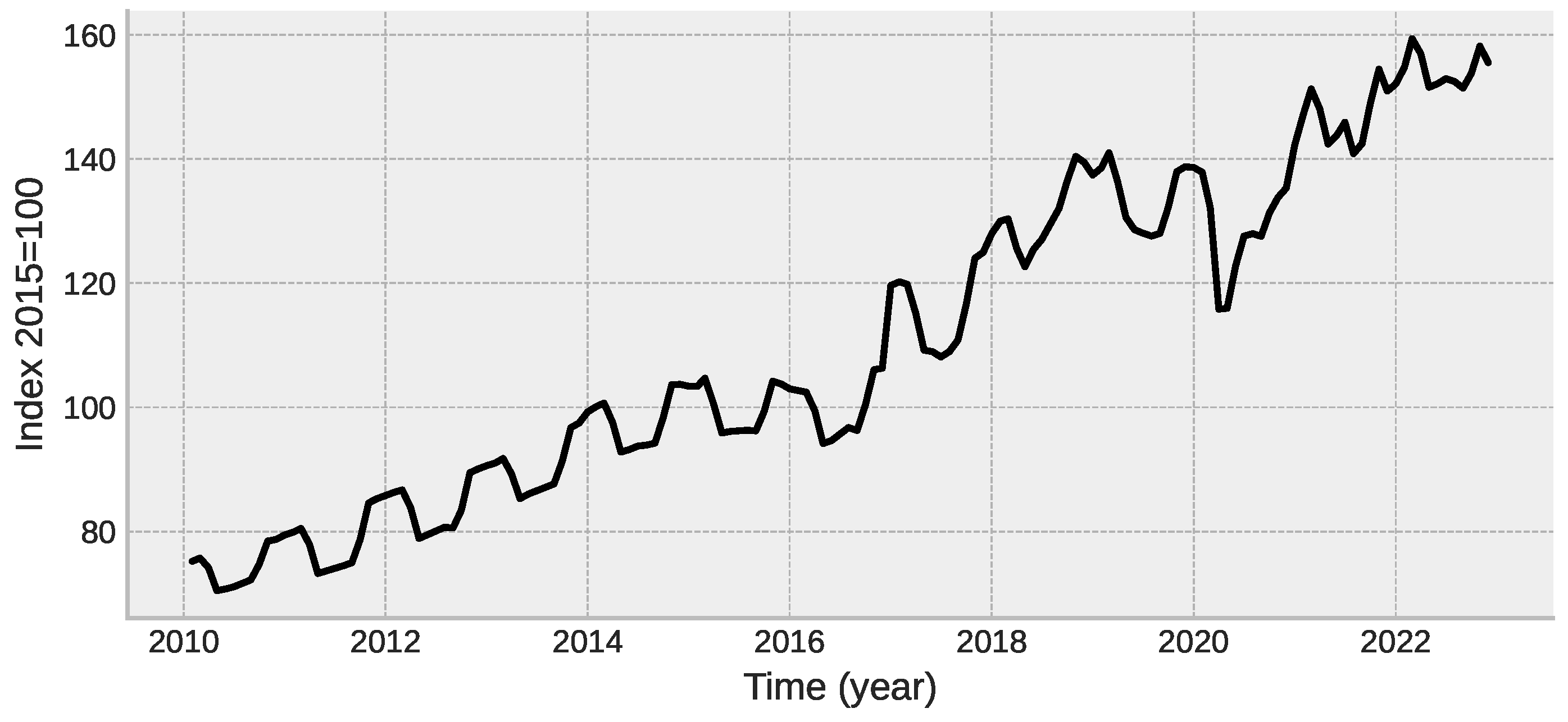
The data used in this paper are from the Organization for Economic Co-operation and Development: Energy for Mexico, retrieved from FRED, Federal Reserve Bank of St. Louis, available at: https://fred.stlouisfed.org/series/MEXCPIENGMINMEI (accessed on 14 February 2023). Additional information can be found in: OECD (2010), “Main Economic Indicators—complete database”, Main Economic Indicators (database), available at: http://dx.doi.org/10.1787/data-00052-en (accessed on 14 February 2023). The variation of energy prices in Mexico over time is presented in Figure 1. For comparative purposes, this variation is normalized (index 2015 = 100).

Figure 1. Original data of the normalized consumer energy price in Mexico.

3.4. Quantile Regression

Quantile regression is a statistical technique that estimates the conditional quantiles of a response variable based on a set of explanatory variables. It is a generalization of ordinary least squares (OLS) regression in which the conditional mean of the response variable is calculated. Let Y represent the response variable, while X represents the explanatory variables. The conditional quantile function $Q_{\tau }\left(Y\right|X)$ of Y at a quantile level $\tau \in (0,1)$ is defined as:

$$\begin{array}{c}\hfill Q_{\tau }\left(Y\right|X)=inf\{y\in \mathbb{R}:P(Y\le y|X)\ge \tau \}\end{array}$$

(17)

where $P(Y\le y|X)$ is the cumulative distribution function of Y given X.

The goal of quantile regression is to estimate the conditional quantile function $Q_{\tau }\left(Y\right|X)$ for a given value of $\tau$ using a linear model, which is achieved by minimizing the following loss function:

$$\begin{array}{c}\hfill \sum _{i=1}^n{\rho }_{\tau }(y_i-x_i^T\beta )\end{array}$$

(18)

where $y_i$ is the observed value of the response variable for the ith observation, $x_i$ is the vector of explanatory variables for the ith observation, $\beta$ is the vector of coefficients to be estimated, and ${\rho }_{\tau }\left(u\right)$ is a function that measures the deviation of u from the quantile of interest $\tau$.

4. Results and Discussion

In this section, the results are discussed, along with an explanation of how the evaluations were conducted and their objectives. Initially, it is explained how the time series is considered for applying the proposed method; after that, the use of SDMA is evaluated, and then the optimized model structure is defined.

4.1. Preparing the Data

In time series analysis, one of the most common tasks is to predict the future values of a time series based on its past behavior. To achieve this, it is necessary to prepare the time series in a suitable way for prediction. A common approach to preparing time series data for prediction is to scale the target variable and create lagged versions of it as features.

The scaling of the target variable is performed to improve the performance of machine learning models on data with large variations. The StandardScaler function from the scikit-learn library is commonly used to normalize the data. The target variable is transformed as follows:

$$\begin{array}{c}\hfill \widetilde{y_t}=\frac{y_t-\mu }{\sigma }\end{array}$$

(19)

where $\widetilde{y_t}$ is the scaled value of the target variable at time t, $y_t$ is the original value of the target variable at time t, $\mu$ is the mean of the target variable, and $\sigma$ is the standard deviation of the target variable.

Creating lagged versions of the target variable as features to capture any time-dependent patterns or trends in the data that might be useful for making predictions. Specifically, the code creates three lagged versions of the target variable, with each lag being a one-time step (month) behind the previous one. These lagged versions of the target variable are denoted as:

$$\begin{array}{c}\hfill y_{t-1},y_{t-2},y_{t-3}.\end{array}$$

(20)

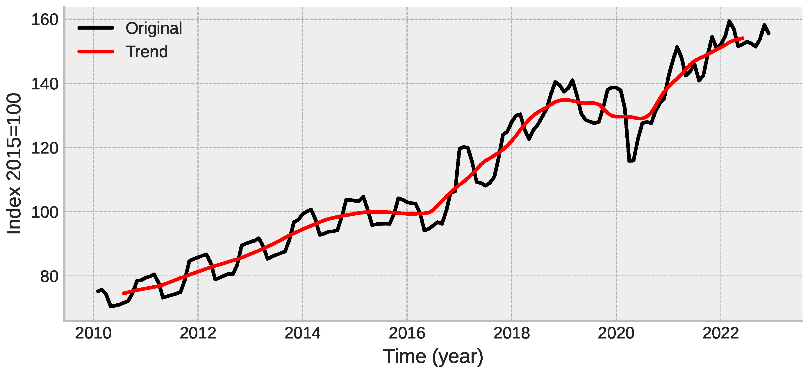
These lagged values of the target variable are then used as input features for machine learning models to predict future values of the time series. Combining scaling the target variable and creating lagged versions of it as features is a common and effective approach to preparing time series data for prediction. Furthermore, we have considered the SDMA output as an extra feature of the model, in order to aid the regressors in making better decisions. The SDMA output is shown in Figure 2 along with the original signal.

Figure 2. Original signal and its trend given by the SDMA filter.

4.2. Single Model Prediction

First, various regression models are evaluated on the prepared time series dataset. This evaluation aims to determine the model that performs best in predicting future values of the time series. R denotes the set of available regressors, where $R=r_1,r_2,\dots ,r_k$. For each regressor, $r_i$ in R, an instance of the regressor class is initialized and fits the prepared time series data. This results in a trained regressor $f_i$ that can be used to predict future time series values.

After training the regressor $f_i$, it is used to predict the target variable on the same dataset using the predict function. The predicted values are compared to the true values of the target variable to calculate the mean squared error (MSE), which measures the average squared difference between the predicted and true values of the target variable. The MSE is calculated as follows:

$$\begin{array}{c}\hfill MSE=\frac{1}{n}\sum _{i=1}^n{(y_i-{\widehat{y}}_i)}^2\end{array}$$

(21)

where $y_i$ is the true value of the target variable at time i, ${\widehat{y}}_i$ is the predicted value of the target variable at time i, and n is the total number of samples in the dataset.

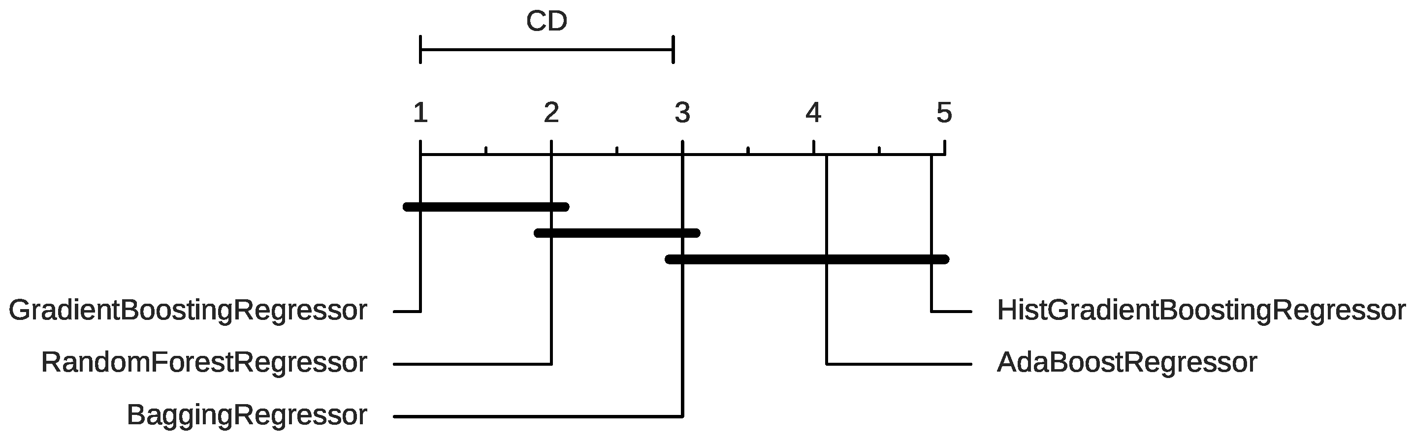
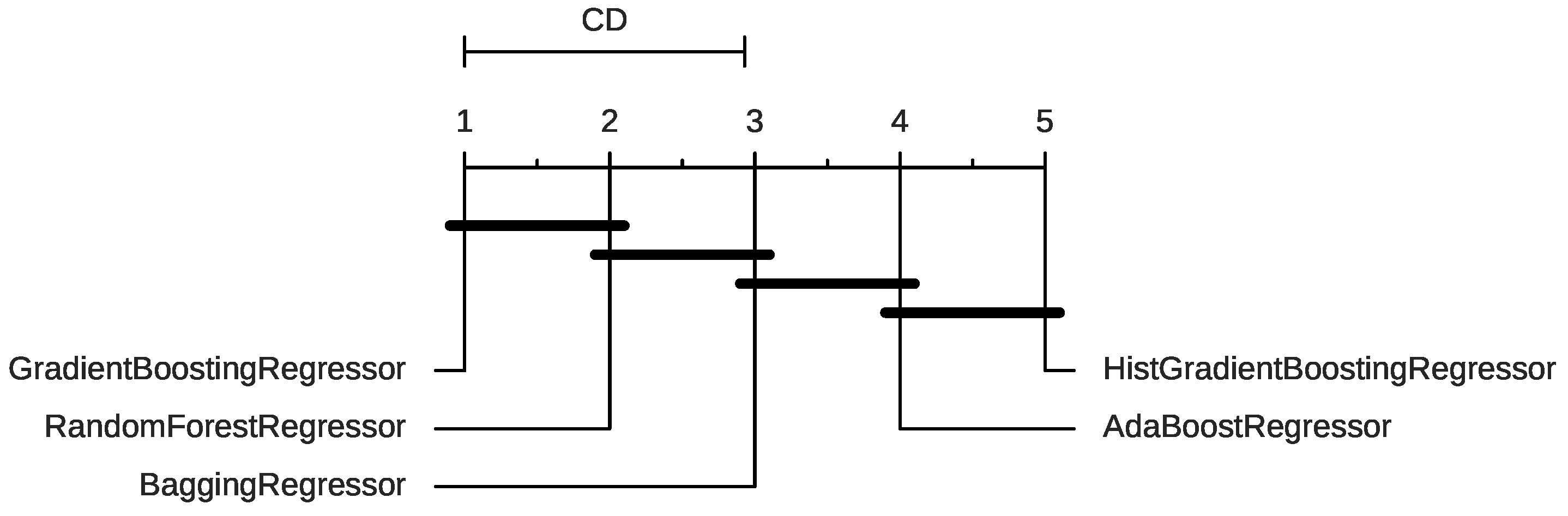
The performance of each regressor $r_i$ is evaluated based on its corresponding MSE. Lower values of MSE indicate better performance of the model on the given data. The name of the regressor $r_i$ and its corresponding MSE are shown in Table 2, while the critical difference diagram for the methods are presented in Figure 3 without SDMA, and in Figure 4 with SDMA.

Table 2. MSE for individual regressors with and without SDMA as an extra feature.

Regressor	MSE without SDMA	MSE with SDMA
AdaBoostRegressor	0.002578	0.001204
BaggingRegressor	0.000904	0.000433
GradientBoostingRegressor	0.000001	0.000001
HistGradientBoostingRegressor	0.004272	0.004059
RandomForestRegressor	0.000256	0.000239

Figure 3. Critical difference diagram for the individual regressors without SDMA.

Figure 4. Critical difference diagram for the individual regressors with SDMA.

4.3. Ensemble Model

This section optimizes hyperparameters for an ensemble model using Optuna, a hyperparameter optimization library. The goal is to find the combination of regressors and their corresponding weights, resulting in the lowest MSE on the prepared time series data. The hyperparameters to optimize include the number of regressors in the ensemble and the choice and weight of each regressor. R denotes the set of available regressors, where $R=r_1,r_2,\dots ,r_k$. The objective function implements the optimization process, which takes a trial object as input. The trial object contains information about the current trial being run by the optimization algorithm.

First, the number of regressors in the ensemble is sampled from a uniform distribution between two and the total number of available regressors. Then, for each regressor, its number of estimators, and weight are sampled from categorical and uniform distributions, respectively. Finally, the number of lagged inputs is also sampled, for a maximum of 20 lagged inputs.

The chosen regressors are then used to initialize instances of their corresponding regressor classes and add them to the ensemble as estimators. The corresponding weights are used to determine the importance of each estimator in making predictions. The ensemble model is trained on the prepared time series data, and the predicted values are compared to the true values of the target variable to calculate the MSE, which is returned by the objective function. During the optimization process, Optuna may prune a trial if it determines that the trial is unlikely to result in a better MSE. This is done by raising the exception when a chosen regressor has already been added to the ensemble twice. The overall procedure is shown in Algorithm 1.   

Algorithm 1: Time Series Prediction using Ensemble Regression

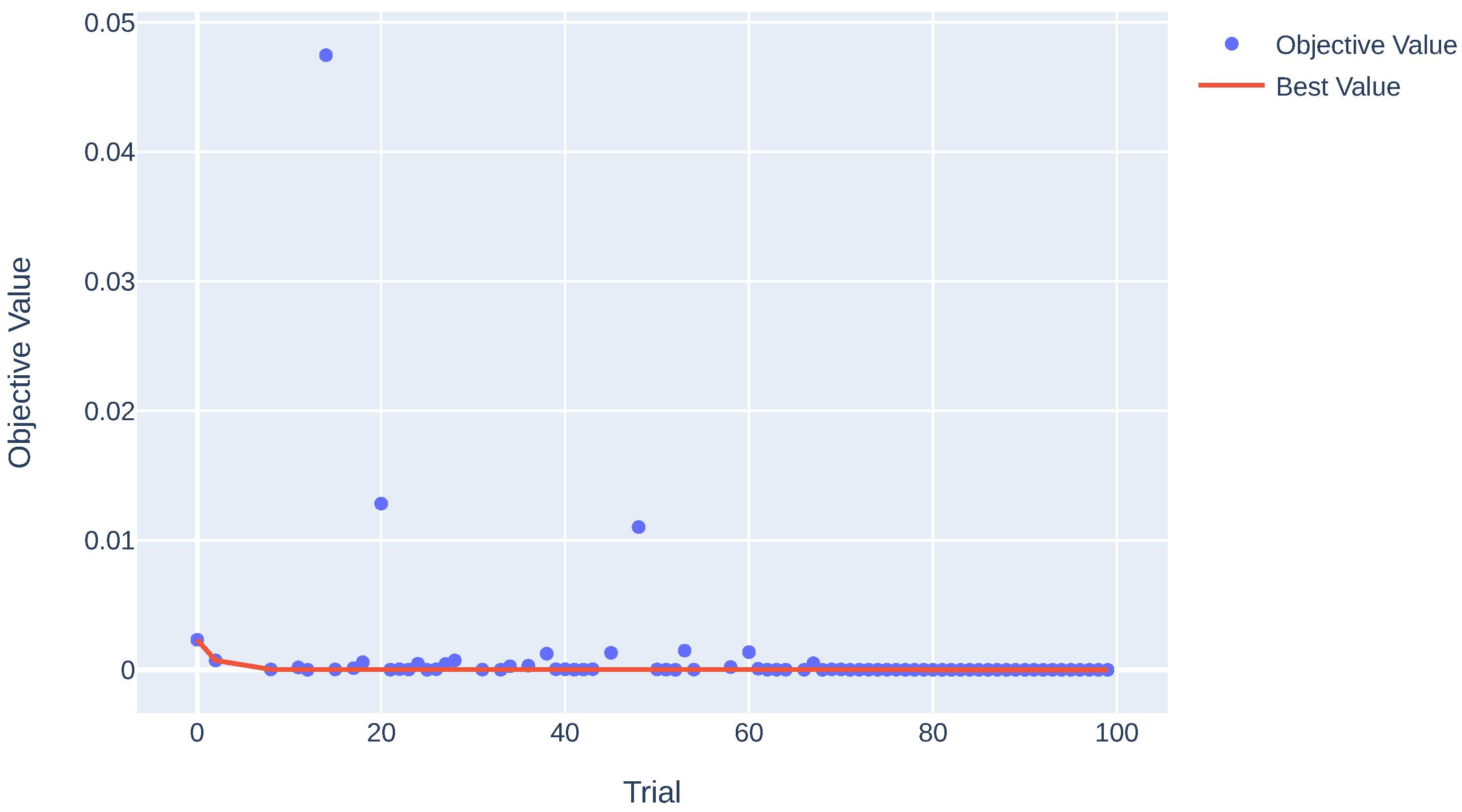
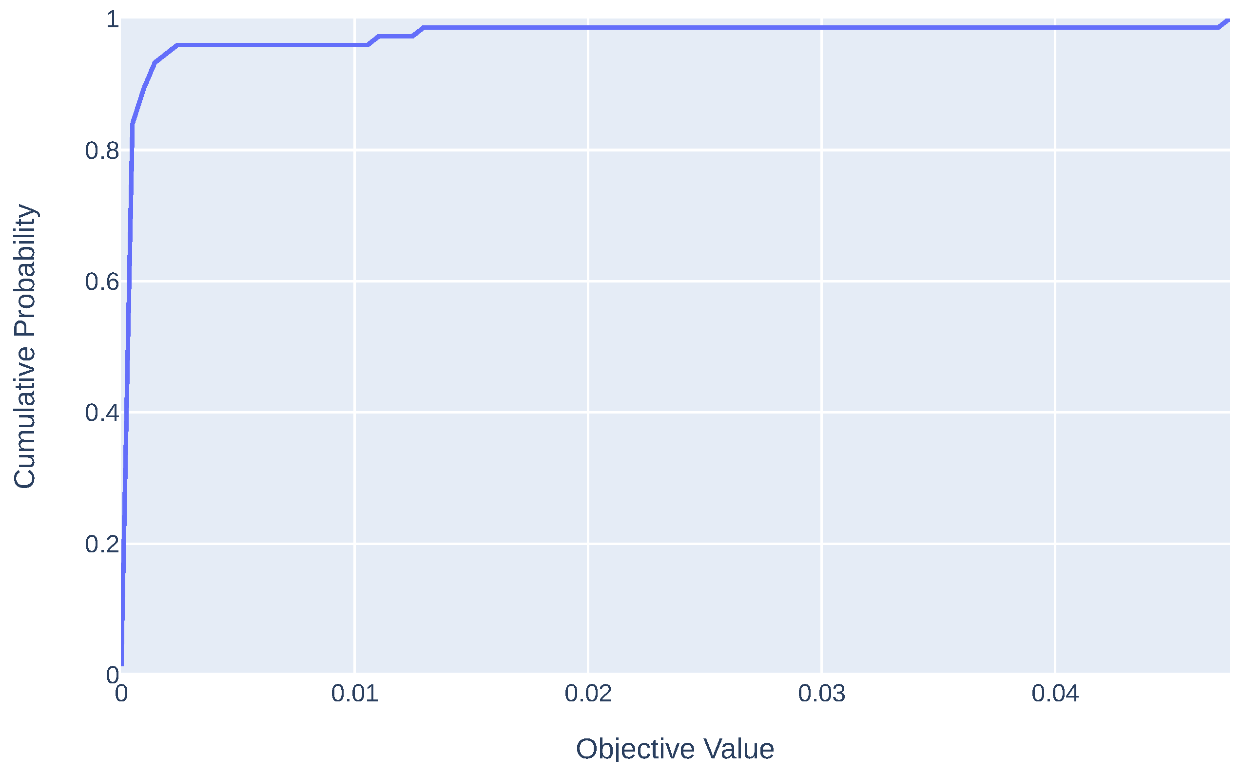
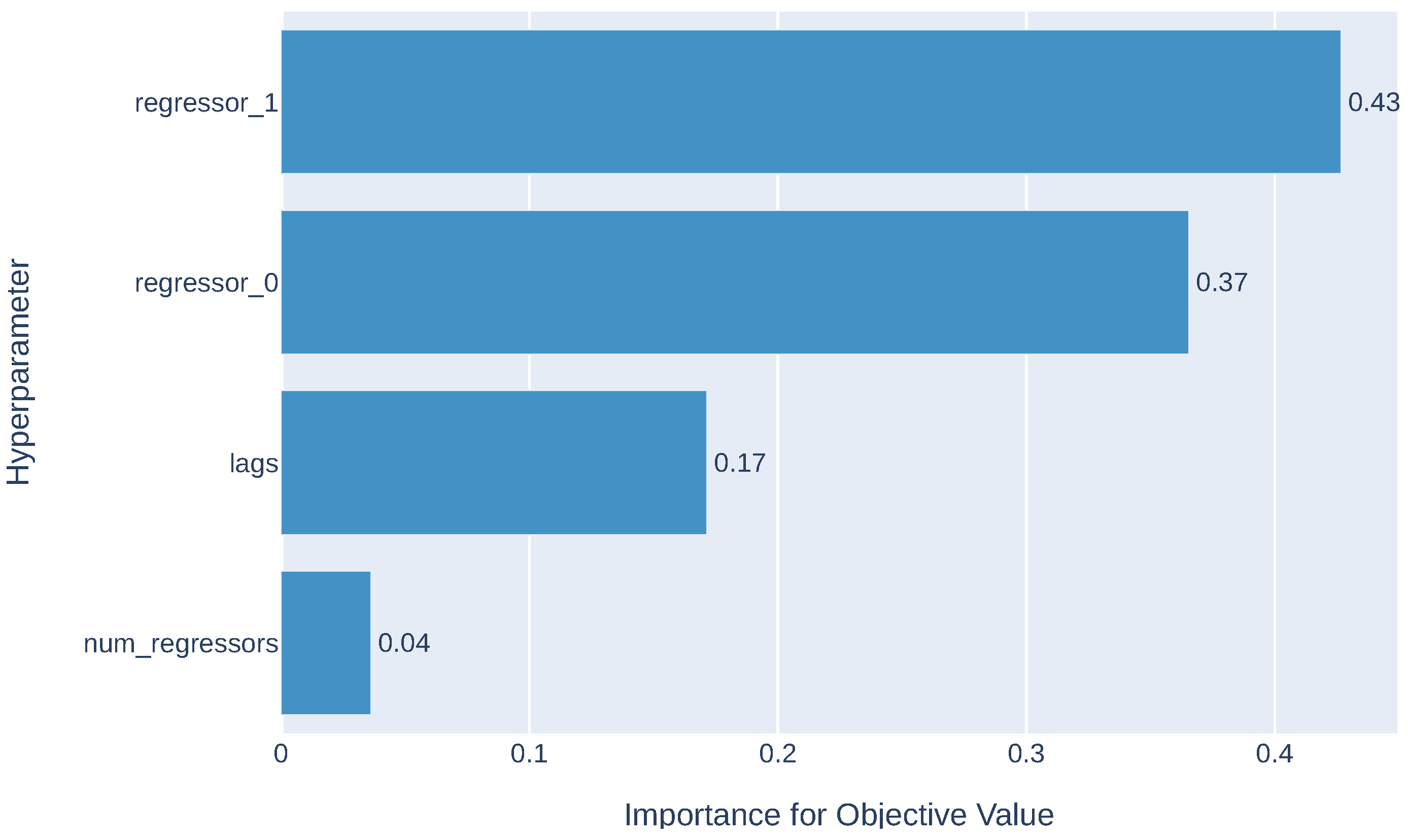
Figure 5 shows the incumbent MSE value along the optimization iterations. Figure 6 presents the procedure’s objective value empirical distribution function (EDF). Finally, Figure 7 shows the importance of each found parameter; it is possible to observe that Optuna has given more importance to varying the chosen regressors than trying to increase the number of regressors.

Figure 5. MSE along the optimization iterations.

Figure 6. Critical difference diagram for the individual regressors.

Figure 7. Importance of the parameters.

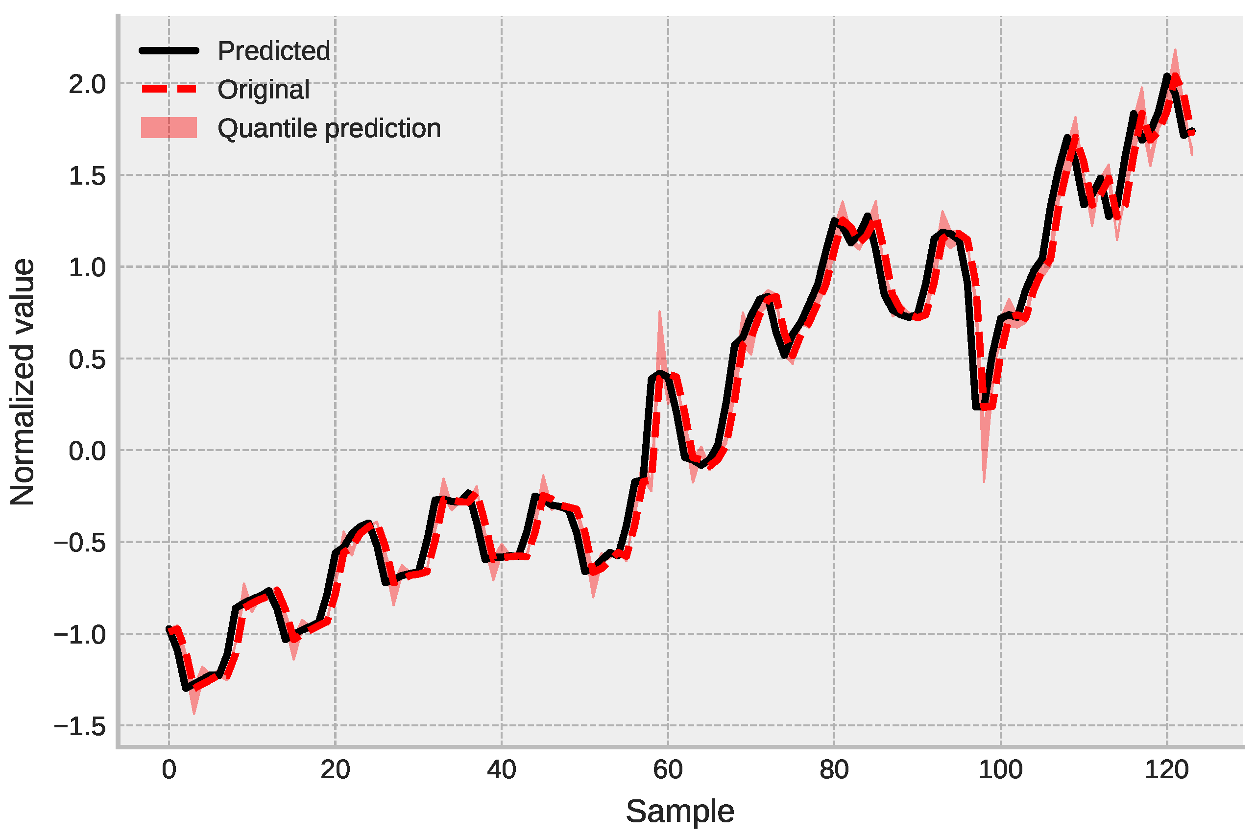
A quantile prediction for the optimized ensemble model is presented in Figure 8, consisting of 2 regressors, namely Histogram-based Gradient Boosting with a learning rate of 0.082 and Gradient Boosting with 456 estimators. A weight of 0.23 was given to the first regressors, while a weight of 0.87 was selected for the second, considering 9 lagged values. This optimized model resulted in an MSE value of $3.375\times {10}^{-9}$ (see Table 3, which presents the MSE results for individual regressors with the SDMA).

Figure 8. Regression and quantile regression of the tuned optimal model.

Table 3. MSE for individual regressors with SDMA as an extra feature, including the proposed model.

Regressor	MSE with SDMA
AdaBoostRegressor	0.001204
BaggingRegressor	0.000433
GradientBoostingRegressor	0.000001
HistGradientBoostingRegressor	0.004059
RandomForestRegressor	0.000239
Proposed Method	3.375 $\times {10}^{-9}$

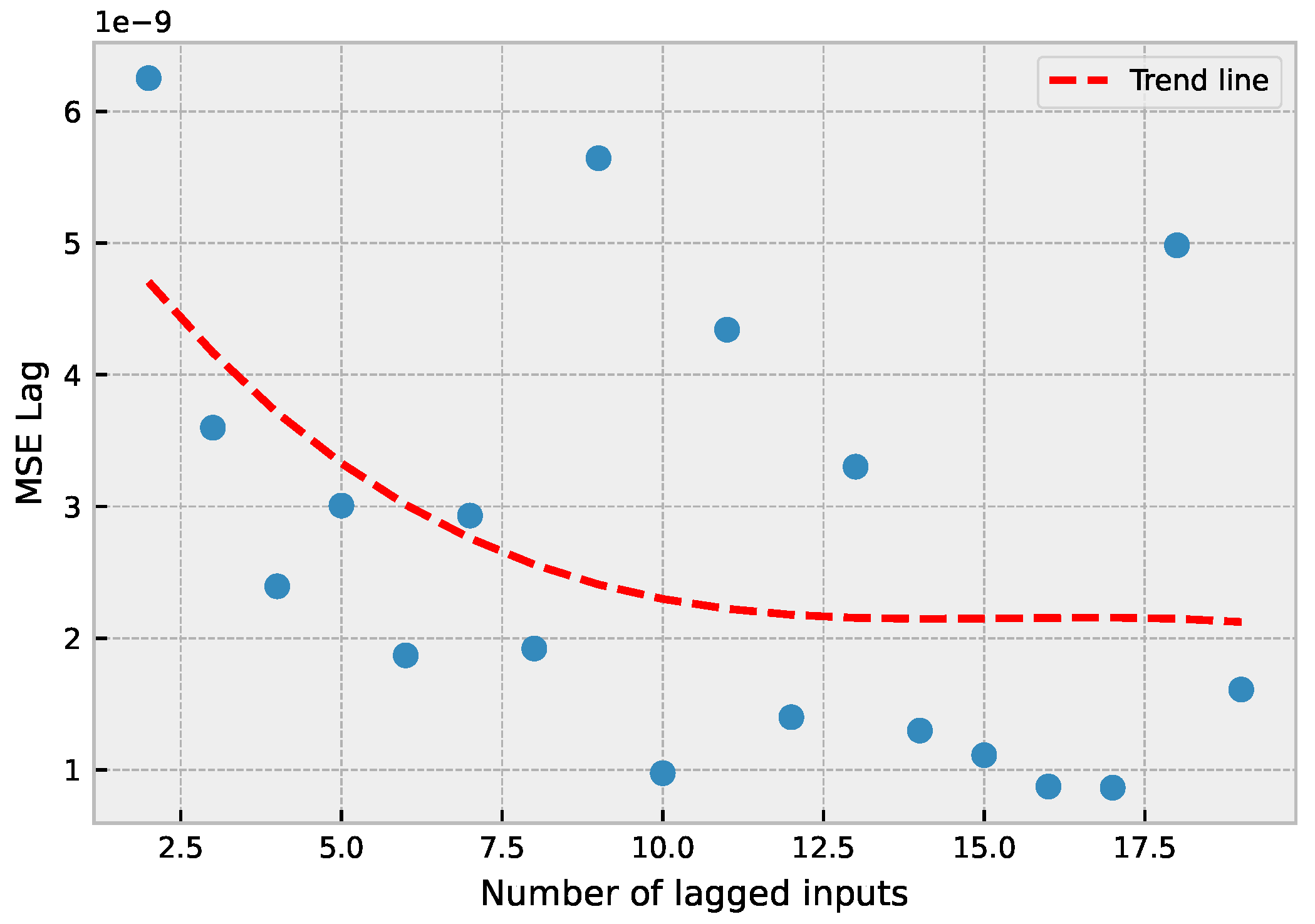
Considering the optimal number of lagged inputs (nine), Table 4 shows the importance of each lagged input in the final prediction. Furthermore, Figure 9 shows the performance of a proposed model as a function of the number of lagged inputs used as input features. The model’s performance is measured in terms of the MSE on a validation set.

Table 4. Feature importance (input lag).

Feature	Feature Importance
Lag 1	0.095993
Lag 2	0.001148
Lag 3	0.000135
Lag 4	0.000135
Lag 5	0.000409
Lag 6	0.000307
Lag 7	0.000116
Lag 8	0.000601
Lag 9	0.031291

Figure 9. MSE Lag × number of lagged inputs.

As the number of lagged inputs increases, the MSE initially decreases rapidly, indicating that including more lagged inputs in the model improves its performance. However, beyond a certain point, adding more lagged inputs results in diminishing returns in terms of the MSE reduction. In fact, for the highest number of lagged inputs, the model’s performance starts to deteriorate, suggesting that the model is overfitting to the training data.

We performed a two-sample t-test to compare the MSE of the predictions generated by the autoregressive integrated moving average (ARIMA) model and the proposed learning method. Let ${\mu }_{\mathrm{ARIMA}}$ and ${\mu }_{\mathrm{Proposed}}$ denote the mean MSE of the ARIMA and proposed methods, respectively. The null hypothesis $H_0:{\mu }_{\mathrm{ARIMA}}={\mu }_{\mathrm{Proposed}}$ assumes that the mean MSE of the two methods is equal. We set the significance level $\alpha =0.05$.

The results of the t-test revealed no significant difference between the mean MSE of the ARIMA model and the proposed learning method ($t\text{-}statistic$ = 0, probabilistic value ($p\text{-}value$) = 0.99). Therefore, we accept the null hypothesis and it is possible to conclude that the two methods are statistically equivalent with respect to their prediction accuracy on the given dataset.

This suggests that both methods perform similarly on this particular problem and dataset and that choosing one method over the other may depend on other factors such as computational efficiency, ease of implementation, or the specific requirements of the application. Nevertheless, further testing on other datasets and scenarios may be necessary to confirm the generalizability of these results.

4.4. Additional Analysis

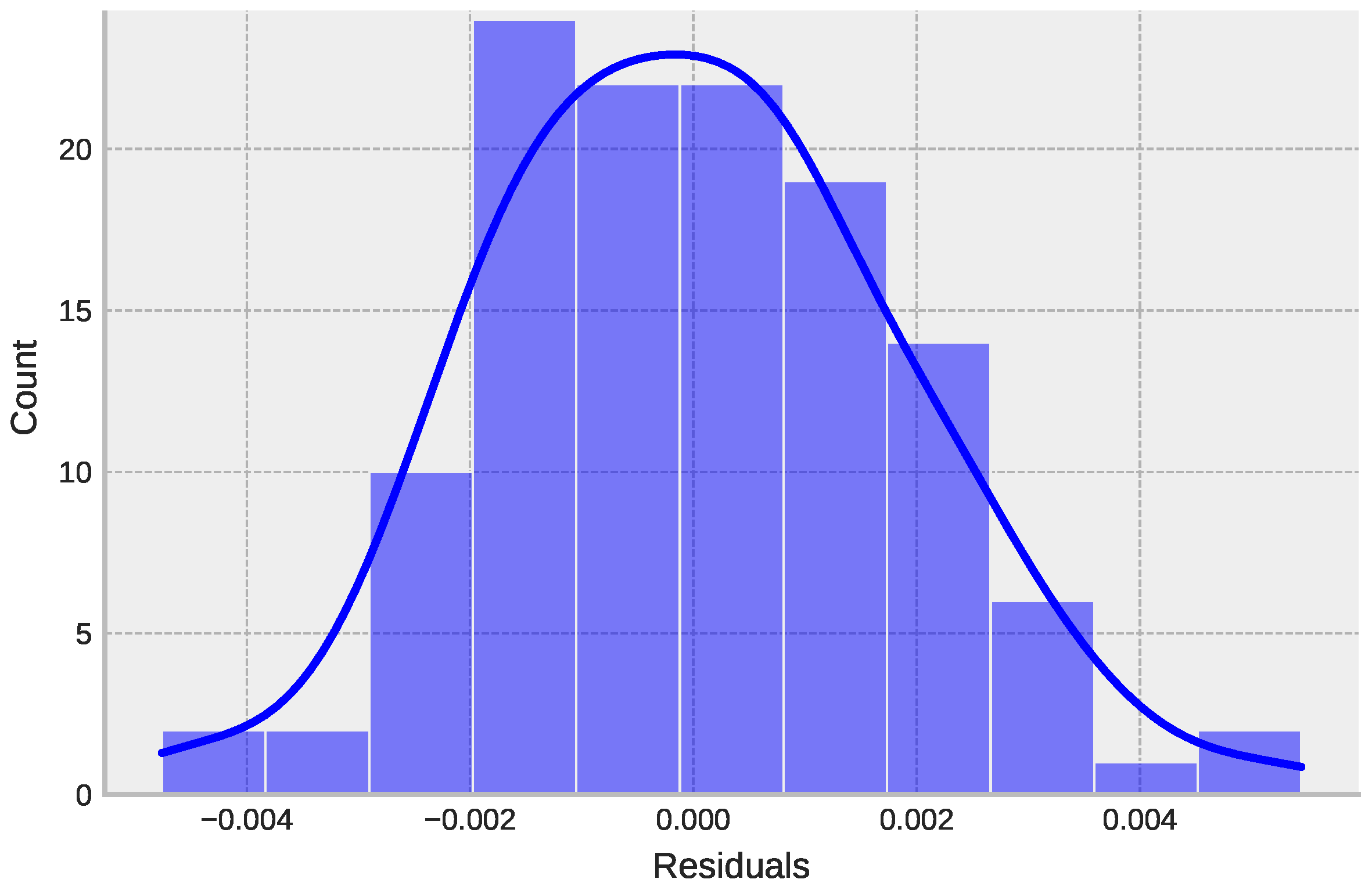
To ensure that the model was capable of dealing with the underlying features of the model, we performed a Shapiro–Wilk test in order to assess the normality of the residuals. As seen in Figure 10, the distribution of the residuals was verified to be normal, i.e., rejecting the null hypothesis that the residues are not normally distributed.

Figure 10. Distribution of the residuals.

Given two signals $x\left(t\right)$ and $y\left(t\right)$, the cross-correlation function $R_{xy}\left(\tau \right)$ measures the similarity between the two signals as a function of time lag $\tau$ as:

$$\begin{array}{c}\hfill R_{xy}\left(\tau \right)={\int }_{-\infty }^{\infty }x\left(t\right)y(t+\tau )dt\end{array}$$

(22)

where the integral is calculated over the entire signal domain. If we have a finite number of data samples, we can estimate the cross-correlation function using the following formula:

$$\begin{array}{c}\hfill R_{xy}\left(\tau \right)=\frac{1}{N}\sum _{n=0}^{N-1}x\left(n\right)y(n+\tau )\end{array}$$

(23)

where N is the number of data samples.

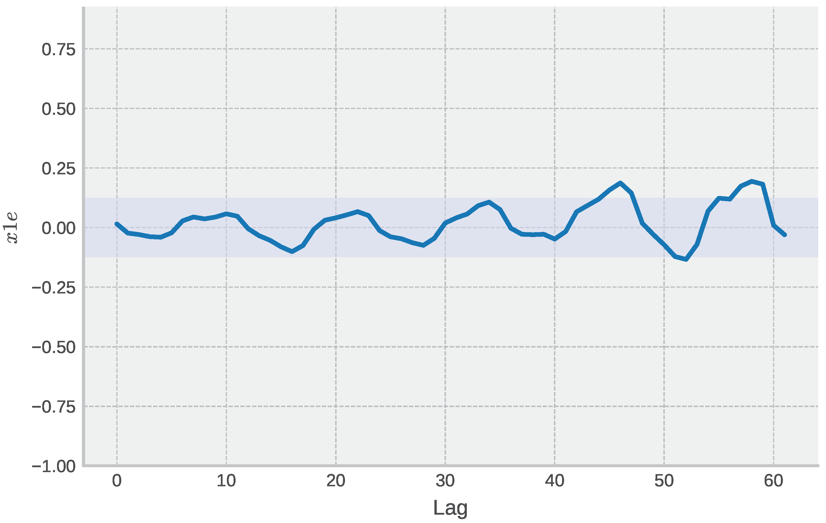
Notice that the cross-correlation function is symmetric, meaning that $R_{xy}\left(\tau \right)=R_{yx}(-\tau )$. Thus, we can further analyze how different input lagged signals can influence the prediction, as shown in Figure 11.

Figure 11. Cross-correlation between the residuals and the input.

5. Final Remarks and Conclusions

The energy price forecast can be a useful indicator for decision-making regarding investment in the industrial sector, and its reduced price assists in social development. For these reasons, analyzing the evolution of energy prices is important to evaluate the direction of public policies that encourage economic and social development. Especially the case study on Mexico is highlighted, as it has one of the lowest energy prices, due to its energy matrix and high development capacity.

The results showed that using SDMA as an extra feature improved the MSE of all the considered ensemble models (AdaBoostRegressor, BaggingRegressor, GradientBoostingRegressor, HistGradientBoostingRegressor, RandomForestRegressor). Combining the models via the Optuna optimization-based voter resulted in a 100 times improvement in error (regarding MSE) compared to the standard ensemble learning methods.

Future work can be accomplished by combining deep learning models using this methodology, in which the computational effort is higher and may result in even more robust and efficient models. The use of the attention mechanism is also something that is worth comparing since several authors have successfully applied it.

References

- Hernández-Fontes, J.V.; Martínez, M.L.; Wojtarowski, A.; González-Mendoza, J.L.; Landgrave, R.; Silva, R. Is ocean energy an alternative in developing regions? A case study in Michoacan, Mexico. J. Clean. Prod. 2020, 266, 121984. [Google Scholar] [CrossRef] [Scilit]
- De La Peña, L.; Guo, R.; Cao, X.; Ni, X.; Zhang, W. Accelerating the energy transition to achieve carbon neutrality. Resour. Conserv. Recycl. 2022, 177, 105957. [Google Scholar] [CrossRef] [Scilit]
- Moshiri, S.; Santillan, M.A.M. The welfare effects of energy price changes due to energy market reform in Mexico. Energy Policy 2018, 113, 663–672. [Google Scholar] [CrossRef] [Scilit]
- Alvarez, J.; Valencia, F. Made in Mexico: Energy reform and manufacturing growth. Energy Econ. 2016, 55, 253–265. [Google Scholar] [CrossRef] [Scilit]
- Wang, Q.; Su, M.; Li, R.; Ponce, P. The effects of energy prices, urbanization and economic growth on energy consumption per capita in 186 countries. J. Clean. Prod. 2019, 225, 1017–1032. [Google Scholar] [CrossRef] [Scilit]
- Qin, L.; Li, W.; Li, S. Effective passenger flow forecasting using STL and ESN based on two improvement strategies. Neurocomputing 2019, 356, 244–256. [Google Scholar] [CrossRef] [Scilit]
- Stefenon, S.F.; Ribeiro, M.H.D.M.; Nied, A.; Mariani, V.C.; Coelho, L.S.; Leithardt, V.R.Q.; Silva, L.A.; Seman, L.O. Hybrid wavelet stacking ensemble model for insulators contamination forecasting. IEEE Access 2021, 9, 66387–66397. [Google Scholar] [CrossRef] [Scilit]
- Ribeiro, M.H.D.M.; Stefenon, S.F.; de Lima, J.D.; Nied, A.; Mariani, V.C.; Coelho, L.d.S. Electricity price forecasting based on self-adaptive decomposition and heterogeneous ensemble learning. Energies 2020, 13, 5190. [Google Scholar] [CrossRef] [Scilit]
- Lehna, M.; Scheller, F.; Herwartz, H. Forecasting day-ahead electricity prices: A comparison of time series and neural network models taking external regressors into account. Energy Econ. 2022, 106, 105742. [Google Scholar] [CrossRef] [Scilit]
- Stefenon, S.F.; Yow, K.C.; Nied, A.; Meyer, L.H. Classification of distribution power grid structures using inception v3 deep neural network. Electr. Eng. 2022, 104, 4557–4569. [Google Scholar] [CrossRef] [Scilit]
- Xie, H.; Zhang, L.; Lim, C.P. Evolving CNN-LSTM models for time series prediction using enhanced grey wolf optimizer. IEEE Access 2020, 8, 161519–161541. [Google Scholar] [CrossRef] [Scilit]
- Shao, Z.; Zheng, Q.; Liu, C.; Gao, S.; Wang, G.; Chu, Y. A feature extraction- and ranking-based framework for electricity spot price forecasting using a hybrid deep neural network. Electr. Power Syst. Res. 2021, 200, 107453. [Google Scholar] [CrossRef] [Scilit]
- Baule, R.; Naumann, M. Volatility and dispersion of hourly electricity contracts on the German continuous intraday market. Energies 2021, 14, 7531. [Google Scholar] [CrossRef] [Scilit]
- Zhang, T.; Tang, Z.; Wu, J.; Du, X.; Chen, K. Short term electricity price forecasting using a new hybrid model based on two-layer decomposition technique and ensemble learning. Electr. Power Syst. Res. 2022, 205, 107762. [Google Scholar] [CrossRef] [Scilit]
- Yang, H.; Schell, K.R. GHTnet: Tri-Branch deep learning network for real-time electricity price forecasting. Energy 2022, 238, 122052. [Google Scholar] [CrossRef] [Scilit]
- Wang, K.; Yu, M.; Niu, D.; Liang, Y.; Peng, S.; Xu, X. Short-term electricity price forecasting based on similarity day screening, two-layer decomposition technique and Bi-LSTM neural network. Appl. Soft Comput. 2023, 136, 110018. [Google Scholar] [CrossRef] [Scilit]
- Wei, J.; Zhang, Y.; Wang, J.; Cao, X.; Khan, M.A. Multi-period planning of multi-energy microgrid with multi-type uncertainties using chance constrained information gap decision method. Appl. Energy 2020, 260, 114188. [Google Scholar] [CrossRef] [Scilit]
- Jiang, P.; Nie, Y.; Wang, J.; Huang, X. Multivariable short-term electricity price forecasting using artificial intelligence and multi-input multi-output scheme. Energy Econ. 2023, 117, 106471. [Google Scholar] [CrossRef] [Scilit]
- Stefenon, S.F.; Seman, L.O.; Mariani, V.C.; Coelho, L.d.S. Aggregating prophet and seasonal trend decomposition for time series forecasting of Italian electricity spot prices. Energies 2023, 16, 1371. [Google Scholar] [CrossRef] [Scilit]
- Klaar, A.C.R.; Stefenon, S.F.; Seman, L.O.; Mariani, V.C.; Coelho, L.S. Optimized EWT-Seq2Seq-LSTM with attention mechanism to insulators fault prediction. Sensors 2023, 23, 3202. [Google Scholar] [CrossRef] [Scilit]
- Branco, N.W.; Cavalca, M.S.M.; Stefenon, S.F.; Leithardt, V.R.Q. Wavelet LSTM for fault forecasting in electrical power grids. Sensors 2022, 22, 8323. [Google Scholar] [CrossRef] [Scilit] [PubMed]
- Sopelsa Neto, N.F.; Stefenon, S.F.; Meyer, L.H.; Ovejero, R.G.; Leithardt, V.R.Q. Fault prediction based on leakage current in contaminated insulators using enhanced time series forecasting models. Sensors 2022, 22, 6121. [Google Scholar] [CrossRef] [Scilit] [PubMed]
- Stefenon, S.F.; Kasburg, C.; Freire, R.Z.; Silva Ferreira, F.C.; Bertol, D.W.; Nied, A. Photovoltaic power forecasting using wavelet neuro-fuzzy for active solar trackers. J. Intell. Fuzzy Syst. 2021, 40, 1083–1096. [Google Scholar] [CrossRef] [Scilit]
- Beltrán, S.; Castro, A.; Irizar, I.; Naveran, G.; Yeregui, I. Framework for collaborative intelligence in forecasting day-ahead electricity price. Appl. Energy 2022, 306, 118049. [Google Scholar] [CrossRef] [Scilit]
- Wang, D.; Gryshova, I.; Kyzym, M.; Salashenko, T.; Khaustova, V.; Shcherbata, M. Electricity price instability over time: Time series analysis and forecasting. Sustainability 2022, 14, 9081. [Google Scholar] [CrossRef] [Scilit]
- Cruz May, E.; Bassam, A.; Ricalde, L.J.; Escalante Soberanis, M.; Oubram, O.; May Tzuc, O.; Alanis, A.Y.; Livas-García, A. Global sensitivity analysis for a real-time electricity market forecast by a machine learning approach: A case study of Mexico. Int. J. Electr. Power Energy Syst. 2022, 135, 107505. [Google Scholar] [CrossRef] [Scilit]
- Rodriguez-Aguilar, R.; Marmolejo-Saucedo, J.A.; Retana-Blanco, B. Prices of Mexican wholesale electricity market: An application of alpha-stable regression. Sustainability 2019, 11, 3185. [Google Scholar] [CrossRef] [Scilit]
- Rehman Javed, A.; Jalil, Z.; Atif Moqurrab, S.; Abbas, S.; Liu, X. Ensemble adaboost classifier for accurate and fast detection of botnet attacks in connected vehicles. Trans. Emerg. Telecommun. Technol. 2022, 33, e4088. [Google Scholar] [CrossRef] [Scilit]
- Khairy, R.S.; Hussein, A.; ALRikabi, H. The detection of counterfeit banknotes using ensemble learning techniques of AdaBoost and voting. Int. J. Intell. Eng. Syst. 2021, 14, 326–339. [Google Scholar] [CrossRef] [Scilit]
- Stefenon, S.F.; Bruns, R.; Sartori, A.; Meyer, L.H.; Ovejero, R.G.; Leithardt, V.R.Q. Analysis of the ultrasonic signal in polymeric contaminated insulators through ensemble learning methods. IEEE Access 2022, 10, 33980–33991. [Google Scholar] [CrossRef] [Scilit]
- Nsaif, Y.M.; Hossain Lipu, M.S.; Hussain, A.; Ayob, A.; Yusof, Y.; Zainuri, M.A.A.M. A new voltage based fault detection technique for distribution network connected to photovoltaic sources using variational mode decomposition integrated ensemble bagged trees approach. Energies 2022, 15, 7762. [Google Scholar] [CrossRef] [Scilit]
- Galicia, A.; Talavera-Llames, R.; Troncoso, A.; Koprinska, I.; Martínez-Álvarez, F. Multi-step forecasting for big data time series based on ensemble learning. Knowl.-Based Syst. 2019, 163, 830–841. [Google Scholar] [CrossRef] [Scilit]
- Guo, R.; Fu, D.; Sollazzo, G. An ensemble learning model for asphalt pavement performance prediction based on gradient boosting decision tree. Int. J. Pavement Eng. 2022, 23, 3633–3646. [Google Scholar] [CrossRef] [Scilit]
- Saha, S.; Saha, M.; Mukherjee, K.; Arabameri, A.; Ngo, P.T.T.; Paul, G.C. Predicting the deforestation probability using the binary logistic regression, random forest, ensemble rotational forest, REPTree: A case study at the Gumani River Basin, India. Sci. Total Environ. 2020, 730, 139197. [Google Scholar] [CrossRef] [Scilit] [PubMed]
- Anjum, M.; Khan, K.; Ahmad, W.; Ahmad, A.; Amin, M.N.; Nafees, A. Application of ensemble machine learning methods to estimate the compressive strength of fiber-reinforced nano-silica modified concrete. Polymers 2022, 14, 3906. [Google Scholar] [CrossRef] [Scilit] [PubMed]
- Sharafati, A.; Asadollah, S.B.H.S.; Al-Ansari, N. Application of bagging ensemble model for predicting compressive strength of hollow concrete masonry prism. Ain Shams Eng. J. 2021, 12, 3521–3530. [Google Scholar] [CrossRef] [Scilit]
- Yang, S.; Wu, J.; Du, Y.; He, Y.; Chen, X. Ensemble learning for short-term traffic prediction based on gradient boosting machine. J. Sens. 2017, 2017, 7074143. [Google Scholar] [CrossRef] [Scilit]
- Lin, S.; Zheng, H.; Han, B.; Li, Y.; Han, C.; Li, W. Comparative performance of eight ensemble learning approaches for the development of models of slope stability prediction. Acta Geotech. 2022, 17, 1477–1502. [Google Scholar] [CrossRef] [Scilit]
- Speiser, J.L.; Miller, M.E.; Tooze, J.; Ip, E. A comparison of random forest variable selection methods for classification prediction modeling. Expert Syst. Appl. 2019, 134, 93–101. [Google Scholar] [CrossRef] [Scilit]
- Chen, D.; Zhang, J.; Jiang, S. Forecasting the short-term metro ridership with seasonal and trend decomposition using LOESS and LSTM neural networks. IEEE Access 2020, 8, 91181–91187. [Google Scholar] [CrossRef] [Scilit]
- Li, Y.; Bao, T.; Gong, J.; Shu, X.; Zhang, K. The prediction of dam displacement time series using STL, extra-trees, and stacked LSTM neural network. IEEE Access 2020, 8, 94440–94452. [Google Scholar] [CrossRef] [Scilit]
- Safaei Pirooz, A.A.; Flay, R.G.; Minola, L.; Azorin-Molina, C.; Chen, D. Effects of sensor response and moving average filter duration on maximum wind gust measurements. J. Wind. Eng. Ind. Aerodyn. 2020, 206, 104354. [Google Scholar] [CrossRef] [Scilit]
Disclaimer/Publisher’s Note: The statements, opinions and data contained in all publications are solely those of the individual author(s) and contributor(s) and not of MDPI and/or the editor(s). MDPI and/or the editor(s) disclaim responsibility for any injury to people or property resulting from any ideas, methods, instructions or products referred to in the content. |
© 2023 by the authors. Licensee MDPI, Basel, Switzerland. This article is an open access article distributed under the terms and conditions of the Creative Commons Attribution (CC BY) license (https://creativecommons.org/licenses/by/4.0/).