Design and Implementation of Predictive Controllers for a 36-Slot 12-Pole Outer-Rotor SPMSM/SPMSG System with Energy Recovery

Abstract

This paper investigates a drive system with energy recovery which uses a 3-phase 1-kW 36-slot 12-pole distributed winding outer-rotor surface-mounted permanent-magnet synchronous motor (SPMSM) and surface-mounted permanent-magnet synchronous generator (SPMSG), which can be used in indoor exercise bicycles. In order to extend drive system operating speed range, the constant torque control, flux-weakening control, and maximum torque/voltage control are used to extend its operation speed up to 1.75 times rated speed. In addition, a predictive speed controller and a predictive current controller are proposed to improve transient responses, load disturbance responses, and tracking responses. A digital signal processor, type TMS-320F-28035, manufactured by Texas Instruments, is used as a control center for the proposed SPMSM/SPMSG drive system. Experimental results validate the feasibility and correctness of the proposed methods.

1. Introduction

Recently, electric indoor exercise bicycles have become more and more popular. Although there has not been much research on these types of bicycles, many researchers have investigated outdoor electric bicycles. For example, Muetze et al. evaluated the performance of different types of electric motor-drive bicycles, including fully electric motor-drive bicycles and partially electric motor-drive bicycles [1]. Chiara reviewed the configurations and performance of different electric bicycles, including surface-mounted permanent-magnet synchronous motors (SPMSM), interior permanent-magnet synchronous motors (IPMSM), and interior permanent-magnet spoke-type motors [2]. Son et al. proposed an SPMSM with independent distributed windings for electric bicycles. In that study, an advance-angle phase-current was implemented to control the torque of the SPMSMs [3]. Misaki et al. implemented an increased power capacity for electric-assisted bicycles using metal hydride fuel cells [4]. Taha designed an inner-rotor and an outer-rotor for electric bicycle applications, and the performance of these two rotor configurations are also compared in this paper [5]. Zhang implemented a low-cost controller for electrical bicycles, in which a sensorless technique was used [6]. Park investigated a position estimation method of an SPMSM drive system for electric bicycles [7]. These previous studies [1,2,3,4,5,6,7], however, only focused on outdoor bicycles but not indoor bicycles.

Several researchers have investigated the predictive controller design and other related control designs for PMSM drive systems. For example, Hammoud et al. proposed continuous-set model predictive control for PMSMs. A real-time realization of a continuous-control-set model predictive current controller for PMSM drive systems was investigated to achieve fast transient responses and good steady-state performance [8]. Eldeeb et al. proposed a unified theory for optimal feedforward torque control of synchronous motor drives. The optimal d-axis current and q-axis current for all operating strategies, including maximum torque per ampere (MTPA), field weakening, maximum torque per voltage (MTPV) were investigated [9]. Hammoud et al. investigated offset-free continuous model predictive current control of PMSM drive systems. A predictive horizon of two steps was achieved with a 100 µs sampling period [10]. Xu et al. proposed a robust predictive current controller with incremental model and inductance observer for PMSM drive systems. In addition, the robustness and disturbance rejection were discussed [11].

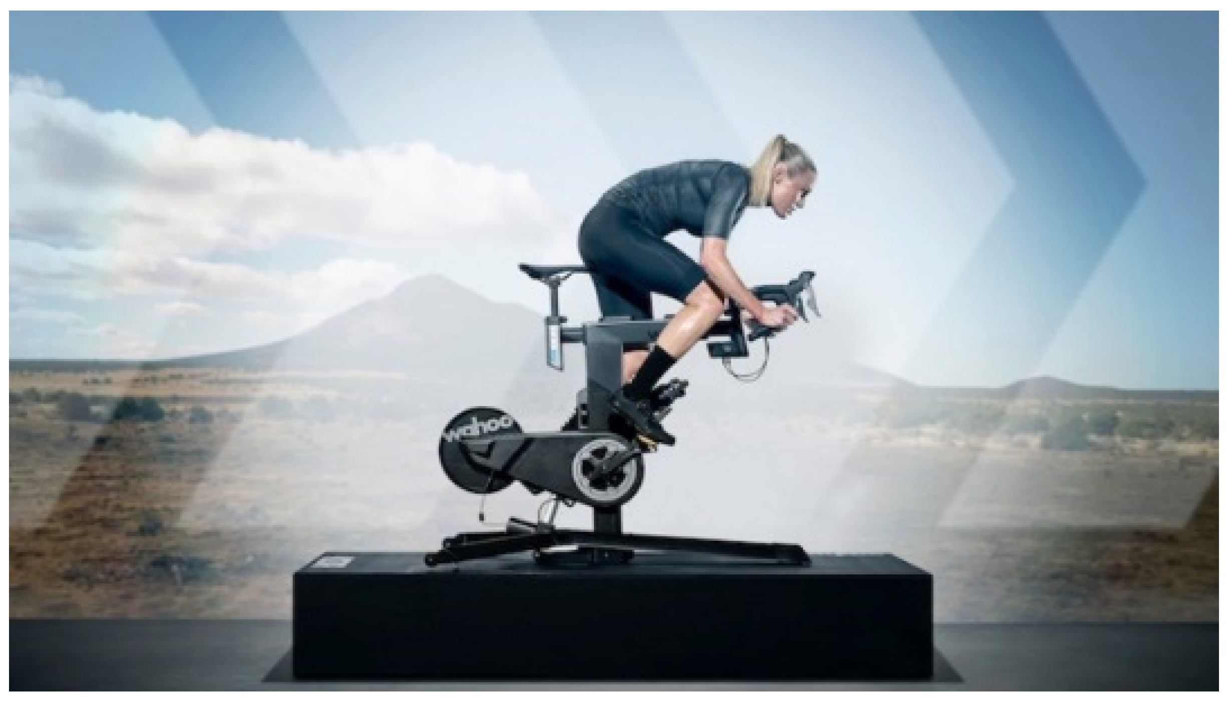
In our paper, the predictive controllers, including a predictive speed controller and a predictive current controller, of the whole drive system using a 36-slot 12-pole outer-rotor SPMSM/SPMSG are investigated for indoor exercise bicycles. An SPMSM/SPMSG drive system for virtual indoor exercise bicycles is implemented to enhance the riders’ pleasure when they use an indoor exercise bicycle. This SPMSM/SPMSG system is implemented to increase the accelerating speed or decelerating speed for the motor of an indoor exercise bicycle. When the rider is riding from a virtual upland to a lowland, the motor of the indoor bicycle is accelerated by adding external torque from the SPMSM drive system. As a result, the riding experience will feel more realistic. When the rider is riding from a virtual lowland to an upland, the motor of the indoor bicycle is decelerated by the braking torque from the SPMSG system. As a result, the rider needs to use more physical force to maintain the speed of the bicycle motor. By using this method, the riders can have a more realistic experience, as though they are riding a standard bicycle outdoors. Figure 1 shows a photograph of the big screen scenarios, which provides a virtual landscape while a rider is riding an indoor bicycle [12]. To the authors’ best knowledge, the ideas of design and implementation of this 36-slot 12-pole outer-rotor SPMSM drive system, which can provide a higher torque and lower speed than a regular 4-pole SPMSM, are original ideas and have not been investigated in the previous papers [1,2,3,4,5,6,7]. In addition, the predictive speed controller and the predictive current controller to enhance the dynamic responses of the SPMSM for indoor bicycle are also new ideas [8,9,10,11]. Finally, the proposed SPMSM drive system does not require any plug-in power from power company. A battery set is used to receive the regenerative energy from riders, and then the battery set provides its energy to the SPMSM drive system to achieve energy saving. These are the three main contributions of this paper.

Figure 1. Photograph of an indoor exercise bicycle with screen.

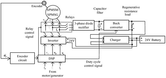
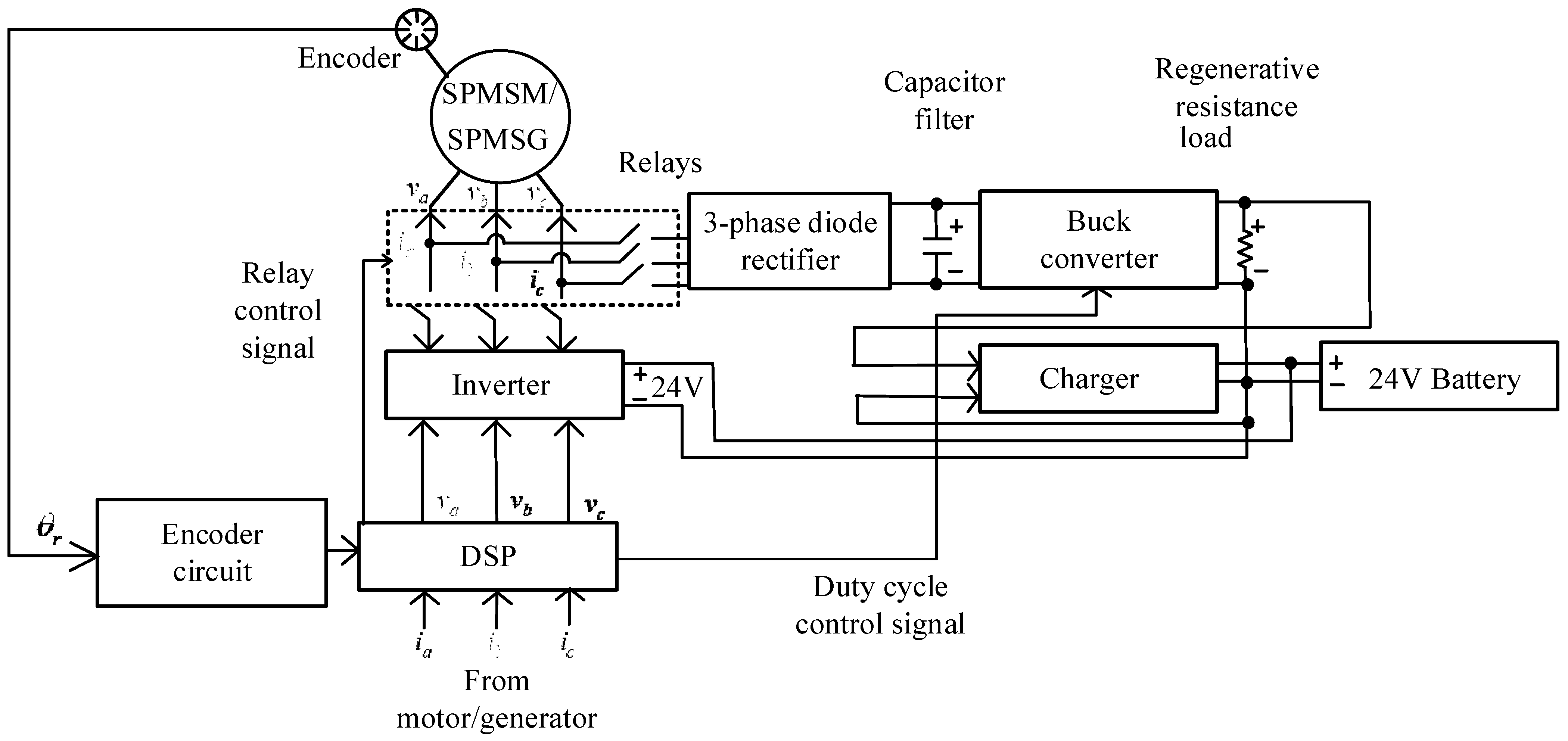
Figure 2 shows the block diagram of the proposed SPMSM/SPMSG system with energy recovery. When the relays are connected to the inverter, the SPMSM is connected to and is controlled by the inverter to operate the SPMSM at different speeds. The SPMSM drive system provides an additional torque to accelerate the motor speed of the bicycle. However, when the relays are connected to the 3-phase diode rectifier, the SPMSG is connected to the rectifier and then to the buck converter, which provides a 25-V output to the regenerative resistance load and also to the charger to charge a 24 V battery set. Improved energy recovery, therefore, is achieved. The digital signal processor (DSP), a 32-bit control center, is used to read the encoder signal and execute the feedback signals, and then control the relays, inverter, buck converter, and charger.

Figure 2. Block diagram of the proposed drive system.

2. Mathematical Model of SPMSMs

The mathematical model of the SPMSM is discussed here. The synchronous d-q axis reference frame of an SPMSM is expressed as follows [13]:

$$\left[\begin{array}{c}{v}_d\\ \\ v_q\end{array}\right]=r_s\left[\begin{array}{c}{i}_d\\ \\ i_q\end{array}\right]+\left[\begin{array}{ccc}{L}_d& & 0\\ & & \\ 0& & L_q^{}\end{array}\right]\frac{d}{dt}\left[\begin{array}{c}{i}_d\\ \\ i_q\end{array}\right]+ {\omega }_e(\left[\begin{array}{ccc}{L}_q& & 0\\ & & \\ 0& & L_d\end{array}\right]\left[\begin{array}{c}-i_q\\ \\ i_d\end{array}\right] + \left[\begin{array}{c}0\\ \\ {\lambda }_m\end{array}\right])$$

(1)

where $v_d$ and $v_q$ are the d-q axis stator voltages, $r_s$ is the stator resistance, $i_d$ and $i_q$ are the d-q axis stator currents, $L_d$ and $L_q$ are the d-q axis inductances, $\frac{d}{dt}$ is the differential operator, ${\omega }_e$ is the electrical rotor speed, and ${\lambda }_m$ is the flux-linkage. The electromagnetic torque is shown as the following equation:

$$T_e=\frac{3}{2}\frac{P}{2}{\lambda }_m^{}{i}_q$$

(2)

where $T_e$ is the electromagnetic torque and $P$ is the pole number.

The speed dynamic equation can be shown as the following equation:

$$\frac{d}{dt}{\omega }_m{=}_{}\frac{1}{J}(T_e-T_L-B{\omega }_m)$$

(3)

where ${\omega }_m$ is the mechanical speed, $J$ is the inertia of the motor and load, $B_{}$ is the viscous coefficient of the motor and load, and $T_L$ is the external load. The electrical rotor position can be expressed as the following equation:

$${\theta }_e=\frac{P}{2}{\theta }_m$$

(4)

where ${\theta }_e$ is the electrical rotor position and ${\theta }_m$ is the mechanical rotor position. Then the mechanical speed ${\omega }_m$ of the motor is shown as follows:

$${\omega }_m=\frac{d}{dt}{\theta }_m$$

(5)

The electrical rotor speed ${\omega }_e$ can now be shown as the following equation:

$${\omega }_e=\frac{P}{2}{\omega }_m$$

(6)

3. Predictive Speed-Loop Controller Design

Predictive control is a kind of control algorithm that was originally applied in industrial processes in the 1970s, and it can be divided into two parts: direct predictive control, which requires a precise model of the uncontrolled plant and indirect predictive control, which involves a lower dimensional model [14]. Unlike many other advanced control methods driven by theoretical research, the development of predictive control was mainly developed by the requirements of industrial practice [15]. Model-based predictive control has several advantages. First, it can be used for multi-input and multi-output systems. Second, it can handle the past, present, and future performances of the dynamics of the system. In addition, predictive control takes account of actuator constraints [16]. Finally, the update rates of predictive control are low; as a result, the predictive control algorithms are easily executed by using a DSP with on-line computations. In this paper, a predictive speed-loop controller and a predictive current-loop controller are designed. The details are discussed as follows.

By using Equation (3) and neglecting $T_L$, we can derive the following equation:

$$T_e=J\frac{d}{dt}{\omega }_m+B{\omega }_m$$

(7)

In addition, from (2), we can obtain the torque equation of the SPMSM, which can be expressed as the following equations:

$$T_e=K_T{i}_q$$

(8)

and

$$K_{\mathrm{T}}=\frac{3}{2}\frac{P}{2}{\lambda }_m$$

(9)

where $K_T$ is the torque constant of the SPMSM. Combining Equations (7) and (8), one can derive the transfer function of the SPMSM as the following equation:

$$G_p(s)=\frac{{\omega }_m(s)}{i_q(s)}=\frac{K_T}{Js+B}$$

(10)

The digital control system proposed in this paper requires a zero-order-hold device to keep the values of the q-axis current. The transfer function of a zero-order-hold device can be expressed as the following equation:

$$G_{s\_zoh}(s)=\frac{1-e^{-s{T}_{st}}}{s}$$

(11)

where $T_{st}$ is the sampling interval of the zero-order-hold device. The cascaded transfer function of the zero-order-hold device and the SPMSM can be rewritten as the following equation:

$$\begin{array}{c}{G}_{zp}(s)=G_{s\_zoh}(s)G_p(s)\\ \hspace{1em}\hspace{1em} =\frac{1-e^{-s{T}_{st}}}{s}\cdot \frac{K_T}{Js+B}\end{array}$$

(12)

By taking the z-transformation, we can obtain the following equation:

$$G_{zp}(z)=\frac{{\omega }_m(z)}{i_q(z)}=\frac{K_T}{B}\left(\frac{1-e^{-\frac{B}{J}{T}_{st}}}{z-e^{-\frac{B}{J}{T}_{st}}}\right)$$

(13)

After that, taking the inverse z-transformation, one can derive the motor speed as the following equation:

$${\omega }_m(k+1)=e^{-\frac{B}{J}{T}_{st}}{\omega }_m(k)+\frac{K_T(1-e^{-\frac{B}{J}{T}_{st}})}{B}{i}_q(k)=a_s{\omega }_m(k)+b_s{i}_q(k)$$

(14)

In Equation (14), the parameters $a_s$ and $b_s$ are defined as the following two equations:

$$a_s=e^{-\frac{B}{J}{T}_{st}}$$

(15)

and

$$b_s=\frac{K_T(1-e^{-\frac{B}{J}{T}_{st}})}{B}$$

(16)

where $a_s$ and $b_s$ are the simplified parameters. By using (k − 1) to replace (k), Equation (14) can be rewritten as the following equation:

$${\omega }_m(k)=a_s{\omega }_m(k-1)+b_s{i}_q(k-1)$$

(17)

Subtracting Equation (17) from Equation (14), one can derive the following equation:

$$\mathrm{\Delta }{\omega }_m(k+1)=a_s\mathrm{\Delta }{\omega }_m(k)+b_s\mathrm{\Delta }{i}_q(k)$$

(18)

where $\mathrm{\Delta }{\omega }_m(k+1)$ is the ${(k+1)}_{th}$ sampling interval difference speed, $\mathrm{\Delta }{\omega }_m(k)$ is the ${(k)}_{th}$ sampling interval difference speed, and $\mathrm{\Delta }{i}_q(k)$ is the ${(k)}_{th}^{}$ sampling interval difference q-axis current. From Equations (17) and (18), we can derive the (k + 1)${}_{th}$ sampling interval estimated speed as the following equation:

$${\widehat{\omega }}_m(k+1)={\omega }_m(k)+a_s\mathrm{\Delta }{\omega }_m(k)+b_s\mathrm{\Delta }{i}_q(k)$$

(19)

After that, we can define the cost function as the following equation [17]:

$$J_p(k)={\left[{\omega }_m^{*}(k+1)-{\widehat{\omega }}_m(k+1)\right]}^2+k_w{\left[\mathrm{\Delta }{i}_q(k)\right]}^2$$

(20)

where $k_w$ is the weighting factor of the cost function of the ${\left[\mathrm{\Delta }{i}_q(k)\right]}^2$. Submitting Equation (19) into Equation (20), we can derive the following equation:

$$\begin{gathered} J_p(k)={\left[{\omega }_m^{*}(k+1)-{\omega }_m(k)-a_s\mathrm{\Delta }{\omega }_m(k)-b_s\mathrm{\Delta }{i}_q(k)\right]}^2+k_w{\left[\mathrm{\Delta }{i}_q(k)\right]}^2 \\ \begin{array}{c}=(b_s^2+k_w){\left[\mathrm{\Delta }{i}_q(k)\right]}^2-2b_s\left[{\omega }_m^{*}(k+1)-{\omega }_m(k)-a_s\mathrm{\Delta }{\omega }_m(k)\right]\mathrm{\Delta }{i}_q(k)+{\left[{\omega }_m^{*}(k+1)-{\omega }_m(k)-a_s\mathrm{\Delta }{\omega }_m(k)\right]}^2\\ \end{array} \end{gathered}$$

(21)

Finally, by taking the $\frac{\partial J_p(k)}{\partial \mathrm{\Delta }{i}_q(k)}$ and assuming that its result equals zero, we can derive the following equation:

$$\frac{\partial J_p(k)}{\partial \mathrm{\Delta }{i}_q(k)}=2(b_s^2+k_w)\mathrm{\Delta }{i}_q(k)-2b_s\left[{\omega }_m^{*}(k+1)-{\omega }_m(k)-a_s\mathrm{\Delta }{\omega }_m(k)\right]=0$$

(22)

From Equation (22) the $\mathrm{\Delta }{i}_q(k)$ can be obtained and expressed as the following equation:

$$\mathrm{\Delta }{i}_q(k)=\frac{b_s\left[{\omega }_m^{*}(k+1)-{\omega }_m(k)\right]-a_s{b}_s\mathrm{\Delta }{\omega }_m(k)}{b_s^2+k_w}$$

(23)

The q-axis current command, therefore, can be expressed as the following equation:

$$i_q^{*}(k)=i_q(k-1)+\mathrm{\Delta }{i}_q(k)$$

(24)

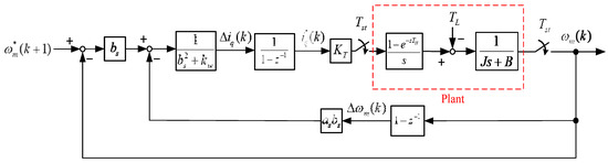
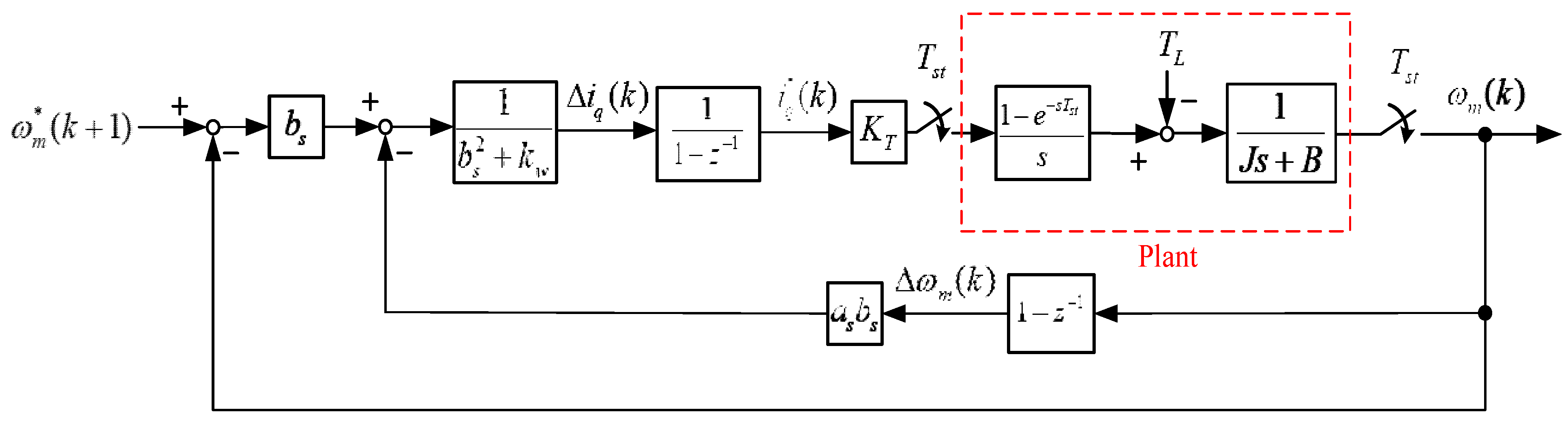
From Equation (23), we can obtain the block diagram of the speed-loop control, which is shown in Figure 3. The control input $i_q^{*}(k)$ is the integration of the $\mathrm{\Delta }{i}_q(k)$, which is a linear combination of the speed error $\left[{\omega }_m^{*}(k+1)-{\omega }_m(k)\right]$ and the $\mathrm{\Delta }{\omega }_m(k)$.

Figure 3. Block diagram of the speed-loop control.

4. Predictive Current-Loop Controller Design

In this section, the details of the predictive current-loop controller design are discussed. From Equation (1), we can obtain the dynamic equation of the d-axis current as follows:

$$\frac{d}{dt}{i}_d=\frac{1}{L_d}(v_d-r_s{i}_d+{\omega }_e{L}_q{i}_q)$$

(25)

From Equation (1), we can obtain the dynamic equation of the q-axis current as follows:

$$\frac{d}{dt}{i}_q=\frac{1}{L_q}\left[v_q-r_s{i}_q-{\omega }_e({\lambda }_m+L_d{i}_d)\right]$$

(26)

The Equations (25) and (26) have coupling terms, which is the electric speed ${\omega }_e$. To simplify the design of the current controller, it is necessary to define the new state variables $u_d$ and $u_q$. The d-q axis current dynamic equations, therefore, can be expressed as the following equations [18]:

$$\frac{d}{dt}{i}_d=\frac{1}{L_d}(u_d-r_s{i}_d)$$

(27)

and

$$\frac{d}{dt}{i}_q=\frac{1}{L_q}(u_q-r_s{i}_q)$$

(28)

In Equation (27) and Equation (28), the variables $u_d$ and $u_q$ are defined as follows:

$$u_d(s)=v_d(s)+{\omega }_e{L}_q{i}_q(s)$$

(29)

and

$$u_q(s)=v_q(s)-{\omega }_e({\lambda }_m+L_d{i}_d(s))$$

(30)

By taking the Laplace transformations of (27) and (28) and combining with (29) and (30), we can derive the following equations:

$$i_d(s)=\frac{v_d(s)+{\omega }_e{L}_q{i}_q(s)}{s{L}_d+r_s}=\frac{u_d(s)}{s{L}_d+r_s}$$

(31)

and

$$i_q(s)=\frac{v_q(s)-{\omega }_e({\lambda }_m+L_d{i}_d(s))}{s{L}_q+r_s}=\frac{u_q(s)}{s{L}_q+r_s}$$

(32)

From Equation (31), we can derive the d-axis current transfer function as follows:

$${\mathrm{G}}_{\mathrm{di}}\left(\mathrm{s}\right)=\frac{i_d(s)}{u_d(s)}=\frac{1}{s{L}_d+r_s}$$

(33)

Then from Equation (32), we can obtain the q-axis current transfer function as follows:

$${\mathrm{G}}_{\mathrm{qi}}\left(\mathrm{s}\right)=\frac{i_q(s)}{u_q(s)}=\frac{1}{s{L}_q+r_s}$$

(34)

In this paper, the d-axis current transfer function is cascaded with a zero-order hold device, and the zero-order hold device has a transfer function which can be shown as follows:

$$G_{c\_zoh}(s)=\frac{1-e^{-s{T}_{ct}}}{s}$$

(35)

where $T_{ct}$ is the sampling interval of the current-loop control. By cascading the zero-order-hold device and the d-axis current transfer function, we can obtain the following equation:

$$G_{zdi}(s)=G_{c\_zoh}(s)G_{di}(s)=\frac{1-e^{-s{T}_{ct}}}{s}\cdot \frac{1}{s{L}_d+r_s}$$

(36)

Similarly, by cascading a zero-order-hold device with the q-axis current transfer function, we can obtain the following equation:

$$G_{zqi}(s)=G_{c\_zoh}(s)G_{qi}(s)=\frac{1-e^{-s{T}_{ct}}}{s}\cdot \frac{1}{s{L}_q+r_s}$$

(37)

By taking the z-transformation of $G_{zdi}(s)$, we can derive the following equation:

$$G_{zdi}(z)=\frac{i_d(z)}{u_d(z)}=\frac{1}{r_s}\left(\frac{1-e^{-\frac{r_s}{L_d}{T}_{ct}}}{z-e^{-\frac{r_s}{L_d}{T}_{ct}}}\right)$$

(38)

Similarly, by taking the z-transformation of $G_{zqi}(s)$, we can derive the following equation:

$$G_{zqi}(z)=\frac{i_q(z)}{u_q(z)}=\frac{1}{r_s}\left(\frac{1-e^{-\frac{r_s}{L_q}{T}_{ct}}}{z-e^{-\frac{r_s}{L_q}{T}_{ct}}}\right)$$

(39)

By taking the inverse z-transformation from Equation (38), we can derive the d-axis dynamic equation as follows:

$$i_d(k+1)=e^{{-}_{}\frac{r_s}{L_d}{T}_{ct}}\cdot i_d(k)+\frac{1-e^{{-}_{}\frac{r_s}{L_d}{T}_{ct}}}{r_s}\cdot u_d(k)$$

(40)

Similarly, by taking the inverse z-transformation from Equation (39), we can derive the q-axis dynamic equation as follows:

$$i_q(k+1)=e^{-\frac{r_s}{L_q}{T}_{ct}}\cdot i_q(k)+\frac{1-e^{-\frac{r_s}{L_q}{T}_{ct}}}{r_s}\cdot u_q(k)$$

(41)

where $i_d(k+1)$ is the ${(k+1)}_{th}$ sampling interval d-axis current and $i_q(k+1)$ is the ${(k+1)}_{th}$ sampling interval q-axis current. From Equation (40), we can rewrite the d-axis current dynamic equation as follows:

$$i_d(k+1)=a_d{i}_d(k)+b_d{u}_d(k)$$

(42)

The parameters in Equation (42) can be defined as follows:

$$a_d=e^{{-}_{}\frac{r_s}{L_d}{T}_{ct}}$$

(43)

and

$$b_d=\frac{1-e^{{-}_{}\frac{r_s}{L_d}{T}_{ct}}}{r_s}$$

(44)

Similarly, from Equation (41), we can rewrite the q-axis current dynamic equation as follows:

$$i_q(k+1)=a_q{i}_q(k)+b_q{u}_q(k)$$

(45)

In Equation (45), we also can define the following two parameters as follows:

$$a_q=e^{{-}_{}\frac{r_s}{L_q}{T}_{ct}}$$

(46)

and

$$b_q=\frac{1-e^{{-}_{}\frac{r_s}{L_q}{T}_{ct}}}{r_s}$$

(47)

Using (k − 1) to replace k, the d-axis and q-axis current dynamic equations can be shown as follows:

$$i_d(k)=a_d{i}_d(k-1)+b_d{u}_d(k-1)$$

(48)

and

$$i_q(k)=a_q{i}_q(k-1)+b_q{u}_q(k-1)$$

(49)

Subtracting (48) from (42), we can derive the following difference equation:

$$\mathrm{\Delta }{i}_d(k+1)=a_d\mathrm{\Delta }{i}_d(k)+b_d\mathrm{\Delta }{u}_d(k)$$

(50)

In addition, subtracting (49) from (45), we can derive the following difference equation:

$$\mathrm{\Delta }{i}_q(k+1)=a_q\mathrm{\Delta }{i}_q(k)+b_q\mathrm{\Delta }{u}_q(k)$$

(51)

where the $\mathrm{\Delta }{i}_d(k+1)$ and $\mathrm{\Delta }{i}_q(k+1)$ are the d-q axis difference currents of the ${(k+1)}_{th}$ sampling interval. The $\mathrm{\Delta }{i}_d(k)$ and $\mathrm{\Delta }{i}_q(k)$ are the d-q axis difference currents of the (k)${}_{th}$ sampling interval. The $\mathrm{\Delta }{u}_d(k)$ and $\mathrm{\Delta }{u}_q(k)$ are d-q axis difference voltages of the (k)${}_{th}$ sampling interval.

From Equation (48) and Equation (50), we can derive the estimated d-axis current of the ${(k+1)}_{th}$ sampling interval as the following equation:

$${\widehat{i}}_d(k+1)=i_d(k)+a_d\mathrm{\Delta }{i}_d(k)+b_d\mathrm{\Delta }{u}_d(k)$$

(52)

From Equation (49) and Equation (51), we can derive the estimated q-axis current of the ${(k+1)}_{th}$ sampling interval as the following equation:

$${\widehat{i}}_q(k+1)=i_q(k)+a_q\mathrm{\Delta }{i}_q(k)+b_q\mathrm{\Delta }{u}_q(k)$$

(53)

Next, we can define the performance index of the d-axis current-loop control as the following equation [18]:

$$J_{cd}(k)={\left[i_d{}^{*}(k+1)-i_d(k)-a_d\mathrm{\Delta }{i}_d(k)-b_d\mathrm{\Delta }{u}_d(k)\right]}^2+k_{cw}{\left[\mathrm{\Delta }{u}_d\left(k\right)\right]}^2$$

(54)

We can also define the performance index of the q-axis current-loop control as the following equation [18]:

$$J_{cq}(k)={\left[i_q{}^{*}(k+1)-i_q(k)-a_q\mathrm{\Delta }{i}_q(k)-b_q\mathrm{\Delta }{u}_q(k)\right]}^2+k_{cw}{\left[\mathrm{\Delta }{u}_q\left(k\right)\right]}^2$$

(55)

where $k_{cw}$ is the weighting factor of the control input $\mathrm{\Delta }{u}_d(k)$ and $\mathrm{\Delta }{u}_q(k)$. From Equation (54), we can rearrange the equation as follows:

$$\begin{array}{l}{J}_{cd}(k)=(b_d^2+k_{cw}){\left[\mathrm{\Delta }{u}_d(k)\right]}^2-2b_d\left[i_d{}^{*}(k+1)-i_d(k)-a_d\mathrm{\Delta }{i}_d(k)\right]\mathrm{\Delta }{u}_d(k)\\ \hspace{1em}\hspace{1em} +\left[i_d{}^{*}(k+1)-i_d(k)-a_d\mathrm{\Delta }{i}_d(k)\right]\\ \end{array}$$

(56)

By using the same method, we can rearrange Equation (55) as follows:

$$\begin{array}{l}{J}_{cq}(k)=(b_q^2+k_{cw}){\left[\mathrm{\Delta }{u}_q(k)\right]}^2-2b_q\left[i_q{}^{*}(k+1)-i_q(k)-a_q\mathrm{\Delta }{i}_q(k)\right]\mathrm{\Delta }{u}_q(k)\\ \hspace{1em}\hspace{1em} +\left[i_q{}^{*}(k+1)-i_q(k)-a_q\mathrm{\Delta }{i}_q(k)\right]\\ \end{array}$$

(57)

Taking $\partial J_{cd}(k)/\partial \mathrm{\Delta }{u}_d(k)$ and assuming that its result equals zero, we can obtain the following equation:

$$2(b_d^2+k_{cw})\mathrm{\Delta }{u}_d(k)-2b_d\left[i_d{}^{*}(k+1)-i_d(k)-a_d\mathrm{\Delta }{i}_d(k)\right]=0$$

(58)

Similarly, taking $\partial J_{cq}(k)/\partial \mathrm{\Delta }{u}_q(k)$ and assuming that its result also equals zero, we can obtain the following equation:

$$2(b_q^2+k_{cw})\mathrm{\Delta }{u}_q(k)-2b_q\left[i_q{}^{*}(k+1)-i_q(k)-a_q\mathrm{\Delta }{i}_q(k)\right]=0$$

(59)

From Equations (58) and (59), we can derive the following two equations:

$$\mathrm{\Delta }{u}_d(k)=\frac{b_d\left(i_d{}^{*}(k+1)-i_d(k)\right)}{b_d^2+k_{cw}}-\frac{a_d{b}_d\mathrm{\Delta }{i}_d(k)}{b_d^2+k_{cw}}$$

(60)

and

$$\mathrm{\Delta }{u}_q(k)=\frac{b_q\left(i_q{}^{*}(k+1)-i_q(k)\right)}{b_q^2+k_{cw}}-\frac{a_q{b}_q\mathrm{\Delta }{i}_q(k)}{b_q^2+k_{cw}}$$

(61)

To consider the real control system, we need to add the coupling terms, $-{\omega }_e{L}_q{i}_q(k)$ and ${\omega }_e\left[{\lambda }_m+L_d\mathrm{\Delta }{i}_d(k)\right]$, and then we can obtain the following equations:

$$\mathrm{\Delta }{v}_d(k)=\mathrm{\Delta }{u}_d(k)-{\omega }_e{L}_q{i}_q(k)$$

(62)

and

$$\mathrm{\Delta }{v}_q(k)=\mathrm{\Delta }{u}_q(k)+{\omega }_e\left[{\lambda }_m+L_d\mathrm{\Delta }{i}_d(k)\right]$$

(63)

where $\mathrm{\Delta }{v}_d(k)$ and $\mathrm{\Delta }{v}_q(k)$ are the differences of the d-q axis control inputs.

Finally, the d-q axis current-loop control inputs can be shown as follows:

$$v_d{}^{*}(k)=v_d(k-1)+\mathrm{\Delta }{v}_d(k)$$

(64)

and

$$v_q{}^{*}(k)=v_q(k-1)+\mathrm{\Delta }{v}_q(k)$$

(65)

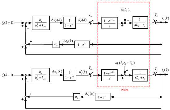
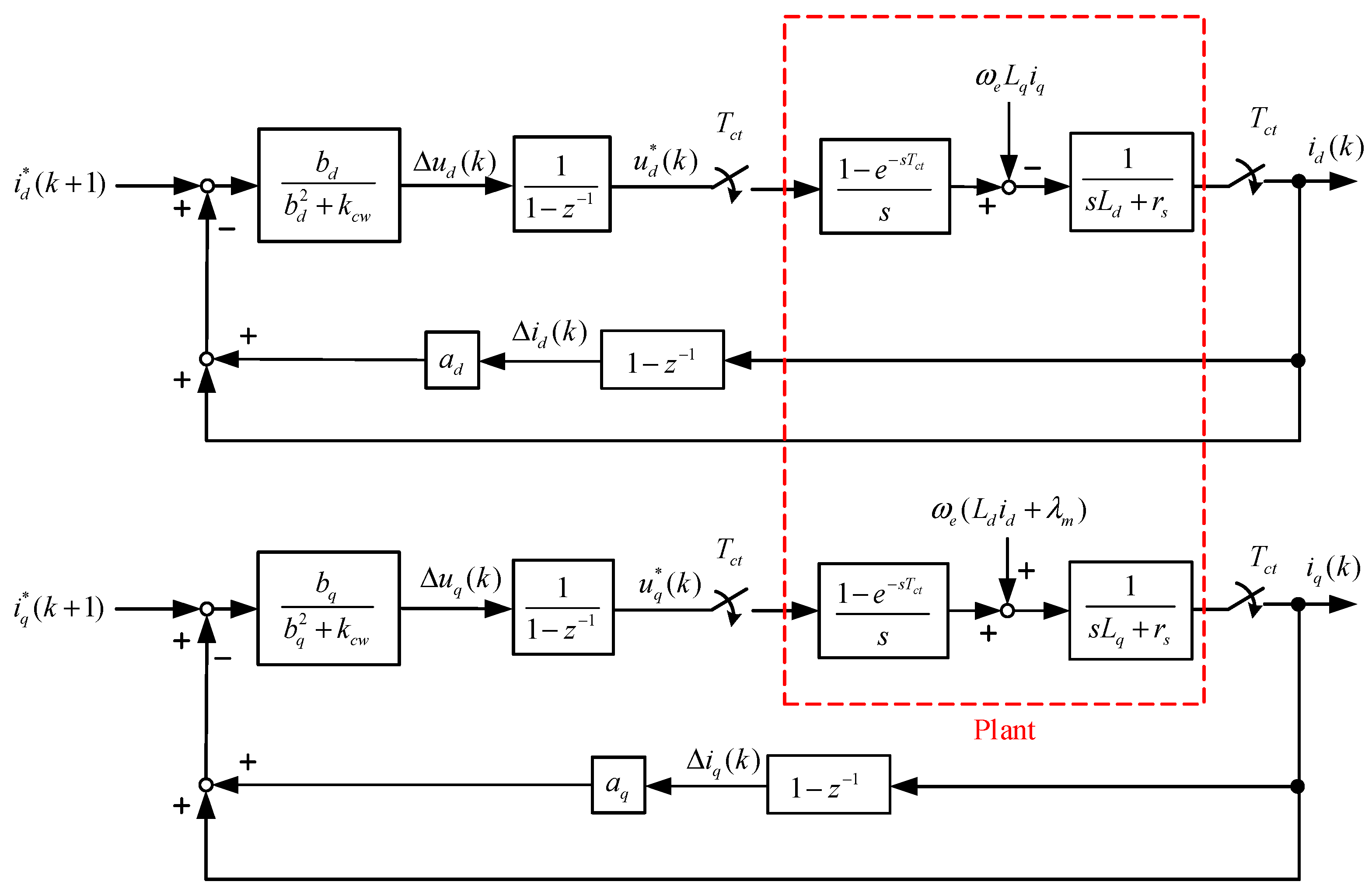
From Equations (60)–(65), we can construct the block diagram of the d-q axis current control system, which is shown in Figure 4. In Figure 4, the q-axis current command is a linear combination of the q-axis current error $[i_q^{*}(k+1)-i_q(k)]$ and $\mathrm{\Delta }{i}_q(k)$. Similarly, the d-axis current command is a linear combination of the d-axis current error $[i_d^{*}(k+1)-i_d(k)]$ and $\mathrm{\Delta }{i}_d(k)$.

Figure 4. Block diagram of the predictive current-loop control.

In this paper, we define a performance index for the d-axis current control, which is shown in Equation (54), and then we also define a performance index for the q-axis current control, which is shown in Equation (55). Next, we use the optimalization technique to solve the $\partial J_{cd}(k)/\partial \mathrm{\Delta }{u}_d(k)$ = 0 and $\partial J_{cq}(k)/\partial \mathrm{\Delta }{u}_q(k)$ = 0. Finally, we calculate the optimal control input $v_d{}^{*}(k)$ and $v_q{}^{*}(k)$. Therefore, we can obtain the optimal current difference $\mathrm{\Delta }{i}_d$ and $\mathrm{\Delta }{i}_q$ for each sampling interval. However, the PI controller only uses pole assignment but not optimization technique to determine ${}_{K_P}$ and ${}_{K_I}$. Moreover, the integral action usually causes delay response. After the d-q coordinate transformation is executed, the $\mathrm{\Delta }{i}_d$ and $\mathrm{\Delta }{i}_q$ generate $\mathrm{\Delta }{i}_a$, $\mathrm{\Delta }{i}_b$, and $\mathrm{\Delta }{i}_c$. As a result, the proposed predictive controller, which uses optimization technique, has smaller harmonic currents than the PI controller does.

5. SPMSM Drive System

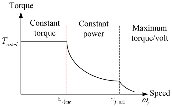
In this paper, a constant DC-link inverter is used. As a result, the SPMSM drive system includes three operating regions: a constant-torque region, a constant-power region, and a maximum-torque per volt region, which are shown in Figure 5 [19]. The details are discussed as follows.

Figure 5. Torque-speed curve of the SPMSM.

(a)

Constant-torque region

When the SPMSM is operated below its rated speed, due to the limits of the motor’s capability, the operating current has to be less than the allowed maximum current, and the operating voltage has to be less than the allowed maximum voltage. As a result, the SPMSM is operated in the constant-torque region. These two constraints are described as the following equations:

$$i_q\le i_q^{\max }$$

(66)

and

$$\sqrt{v_d^2+v_q^2}\le v_s^{\max }$$

(67)

where $i_q^{\max }$ is the maximum q-axis current and $v_s^{\max }$ is the maximum stator voltage.

(b)

Constant-power region

When the PMSM is operated beyond its rated speed, the back-EMF is increased and is close to the DC-bus voltage. In this situation, the resistance voltage drop and the inductance voltage drop are neglected. By submitting $r_s{i}_q=0,$ $i_d$ = 0, and $\frac{d}{dt}{L}_q{i}_q=0$ into Equation (1), we can derive the following equations:

$$v_d=-{\omega }_e{L}_q{i}_q$$

(68)

and

$$v_q={\omega }_e{\lambda }_m$$

(69)

Then, by submitting (68) and (69) into (67), we can obtain the following equation:

$$\sqrt{{(-{\omega }_e{L}_q{i}_q)}^2+{({\omega }_e{\lambda }_m)}^2}\le v_s^{\max }$$

(70)

From Equation (70), we can easily derive the following equation:

$$(i_s^{sc}{)}^2+{i_q}^2\le (\frac{v_s^{\max }}{{\omega }_e{L_q}^2})$$

(71)

where $i_s^{sc}$ is defined as $\left(\frac{{\lambda }_m}{L_q}\right),$ which is the characteristic current of the SPMSM.

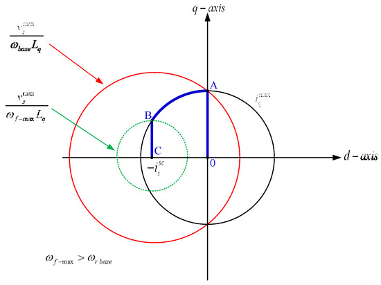
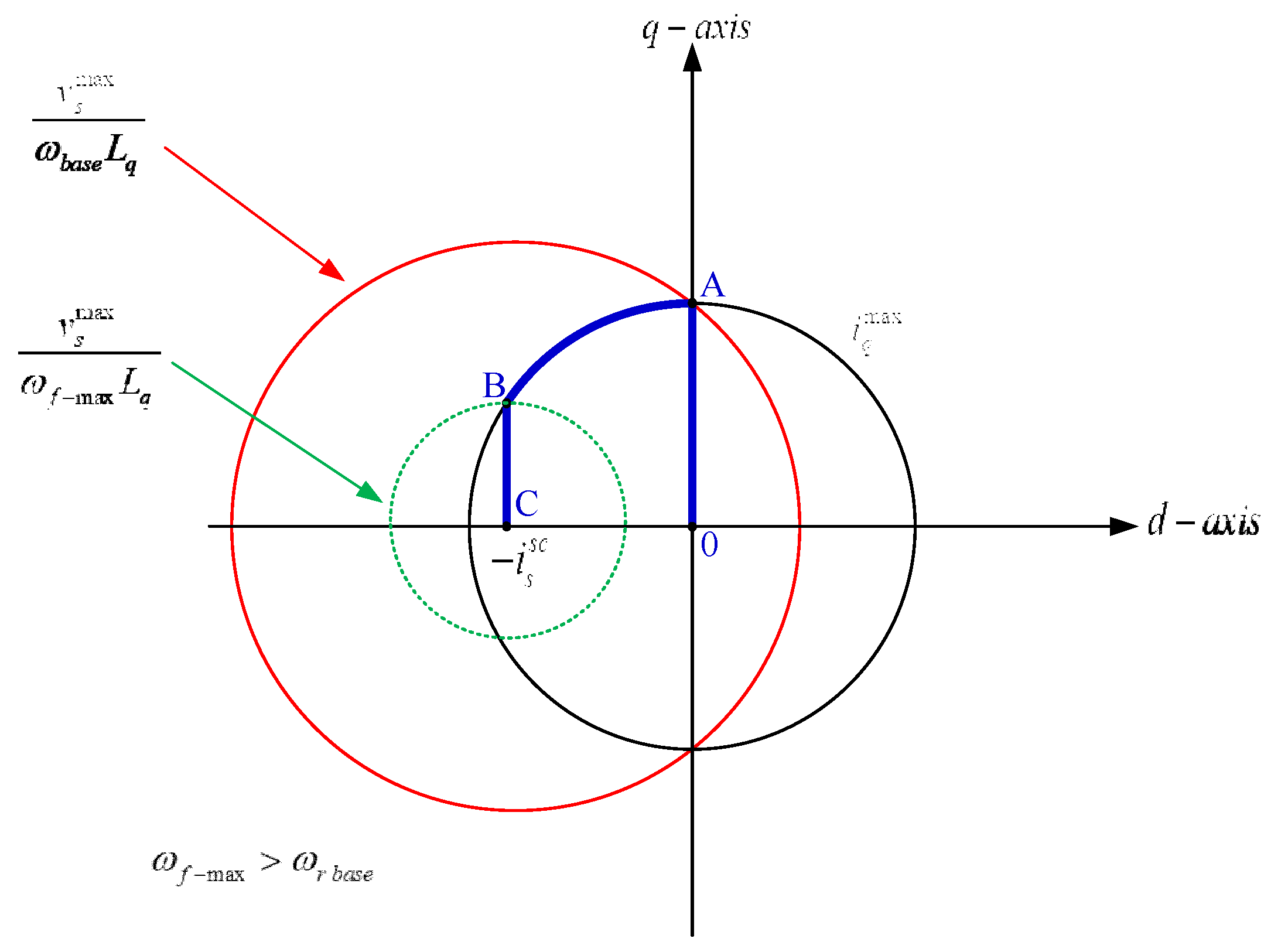
The Equation (71) can be graphically expressed and is shown in Figure 6, which includes a current constraint and a voltage constraint. In Figure 6, the line OA is the constant torque region, the line AB is the constant power region, and the line BC is the maximum torque/volt region.

Figure 6. The d-q axis current curves. The line from 0 to A is MTPA control, and the line from A to B is Flux-weakening control.

(c)

Maximum torque/volt control region

When the SPMSM is operated at the B point in Figure 6, the d-axis current is near $i_s^{sc}$, there is little flux, which causes serious current harmonics, and then this deteriorates the performance of the SPMSM. To solve this problem, in this paper, a maximum torque per volt (MTPV) method is used, which decreases the q-axis current to decrease the torque. The d-q axis currents can now be shown as follows:

$$i_{d\_\mathrm{MTPV}}=-i_s^{sc}$$

(72)

and

$$i_{q\_\mathrm{MTPV}}=\frac{v_s^{\max }}{{\omega }_e{L}_q}$$

(73)

where $i_{d\_\mathrm{MTPV}}$ is the d-axis current in the MTPV operating region, and $i_{q\_\mathrm{MTPV}}$ is the q-axis current in the MTPV operating region.

(d)

Implementation

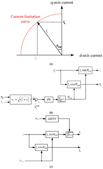
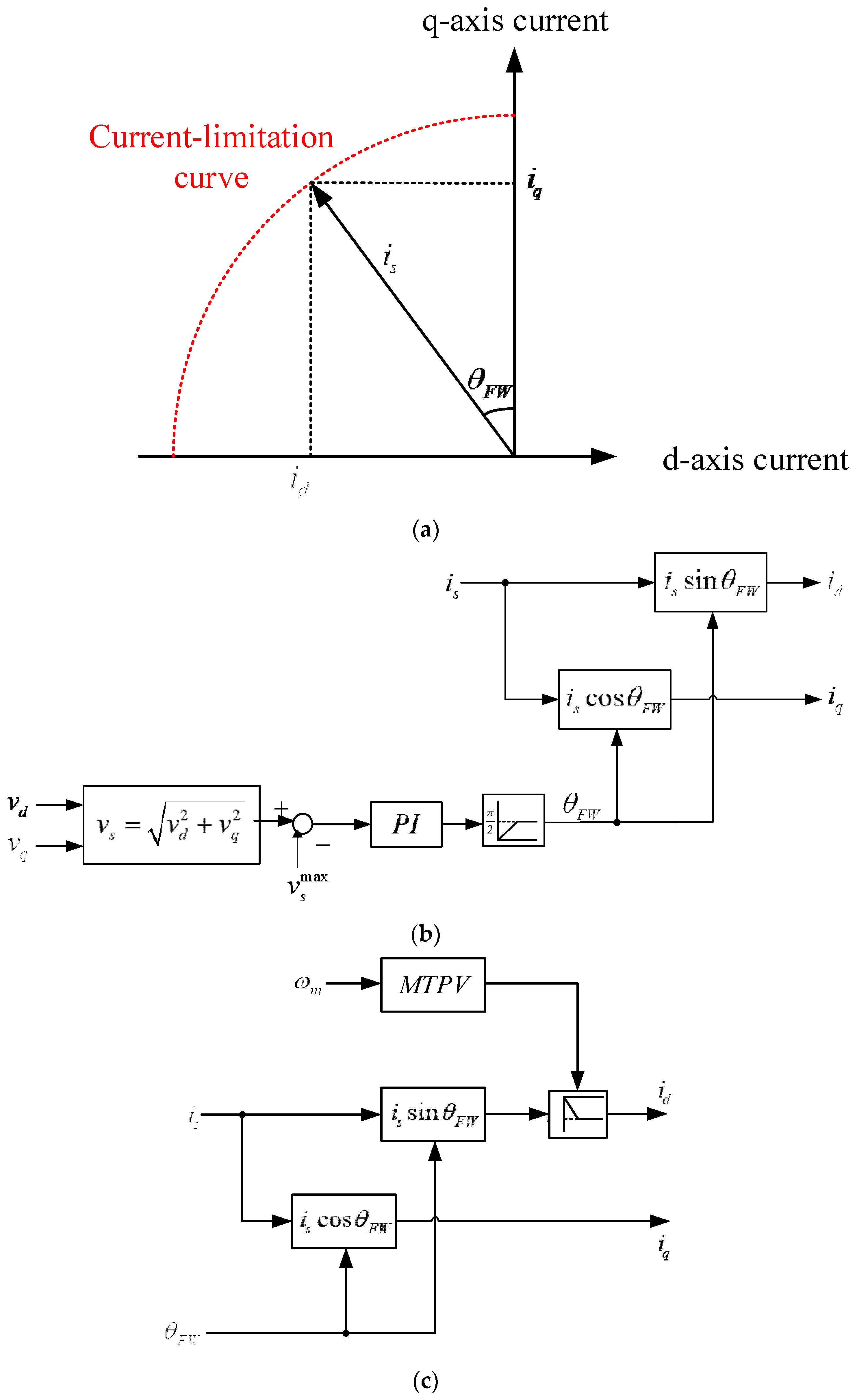
In this paper, an advance angle control is used to control the current vector $i_s$, which is shown in Figure 7a. When the SPMSM is operated in the constant torque region, the advance angle ${\theta }_{FW}$ is set as zero. However, when the SPMSM is operated in the constant power region, the ${\theta }_{FW}$ is gradually increased. As a result, the d-axis becomes more negative and the q-axis current is gradually reduced, and this is shown in Figure 7b. When the SPMSM is operated in the MTPV operating region, the d-axis current is fixed, and then the q-axis current is gradually reduced, and this is shown in Figure 7c.

Figure 7. Flux-weakening and MTPV control. (a) d-q axis current curve, (b) flux-weakening control, (c) MTPV control.

6. Implementation

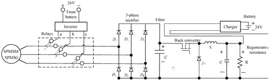
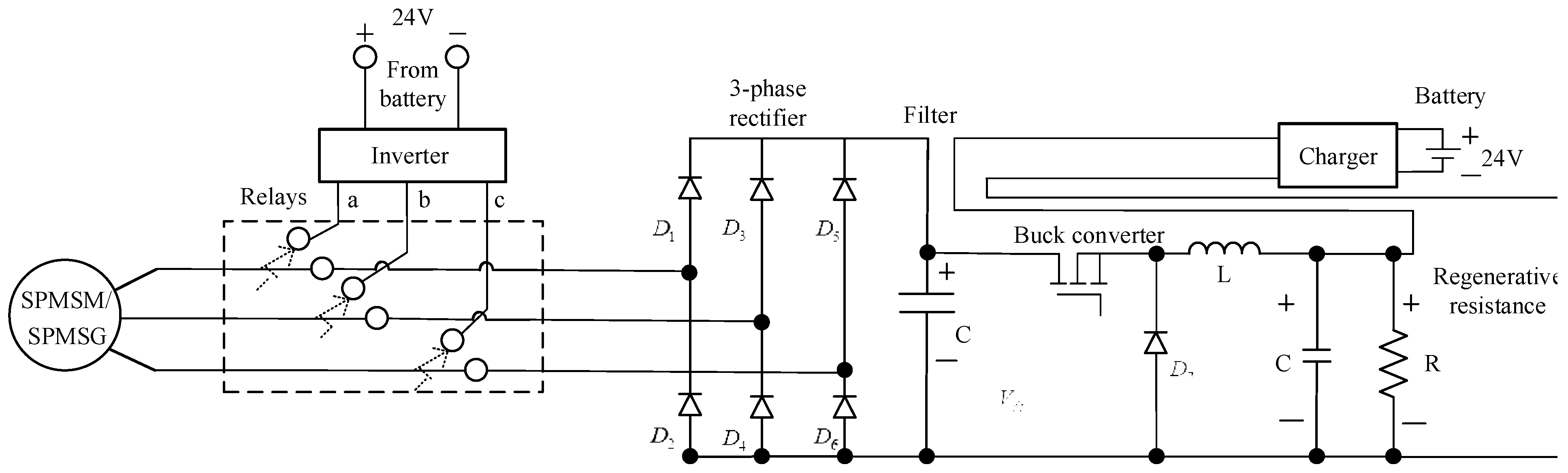
Figure 8 shows the implemented regeneration circuit of the SPMSM drive system. The SPMSM/SPMSG has a rated speed of 200 r/min, 36 slots, 12 poles, a stator resistance of 6.84 Ω, d-axis and q-axis inductances of 9.8 mH, a flux linkage of 0.122 V·s/rad, an inertia of 0.01 kg·m², and a viscous coefficient of 0.005 N·m·s/rad. When the indoor exercise bicycle is ridden from a virtual upland to a lowland, the motor of the indoor exercise bicycle is accelerated. Then, the relays are connected to the inverter, which uses the energy from the battery set to drive the SPMSM, which adds extra torque to the indoor exercise bicycle to make the ride feel more realistic. However, when the rider of the indoor bicycle is riding from a virtual lowland to an upland, the motor of the indoor exercise bicycle is decelerated. The relays are connected to the 3-phase rectifier to transfer the SPMSG energy to the capacitor of the DC-link. After that, a buck-converter is used to convert the DC-link capacitor voltage to near 25 V, which provides for regenerative resistance. Then, the SPMSM converter transforms its energy into the regenerative resistance. In order to store and save the recovered energy, a charger is implemented to use the regenerated energy to charge the 24-V battery set.

Figure 8. Implemented regeneration circuit of the PMSM drive system.

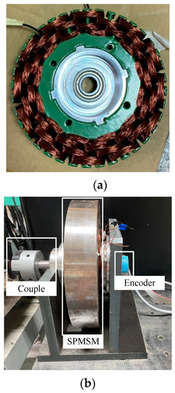
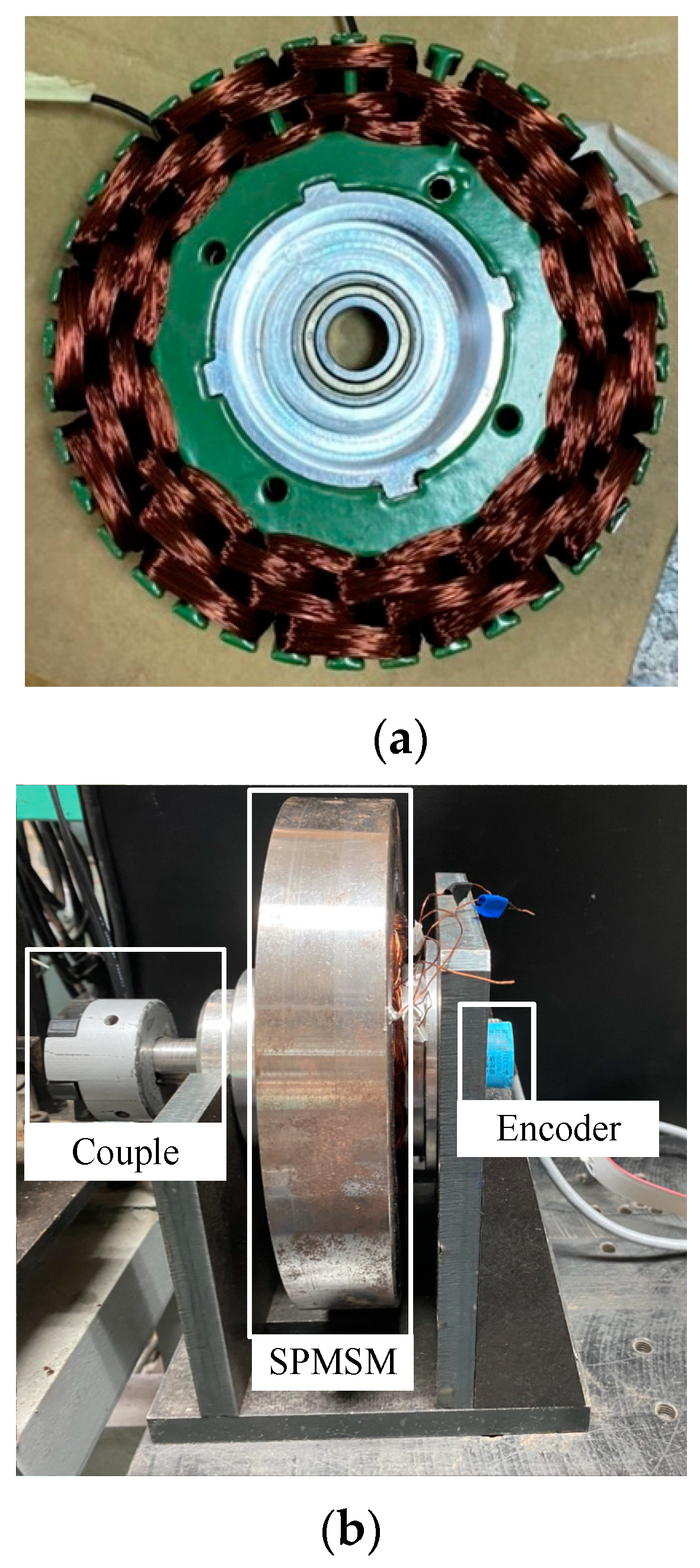
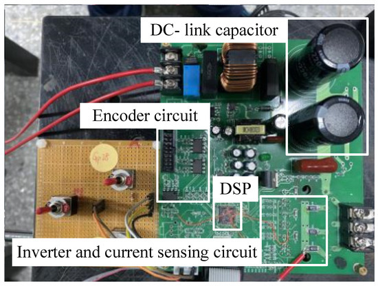
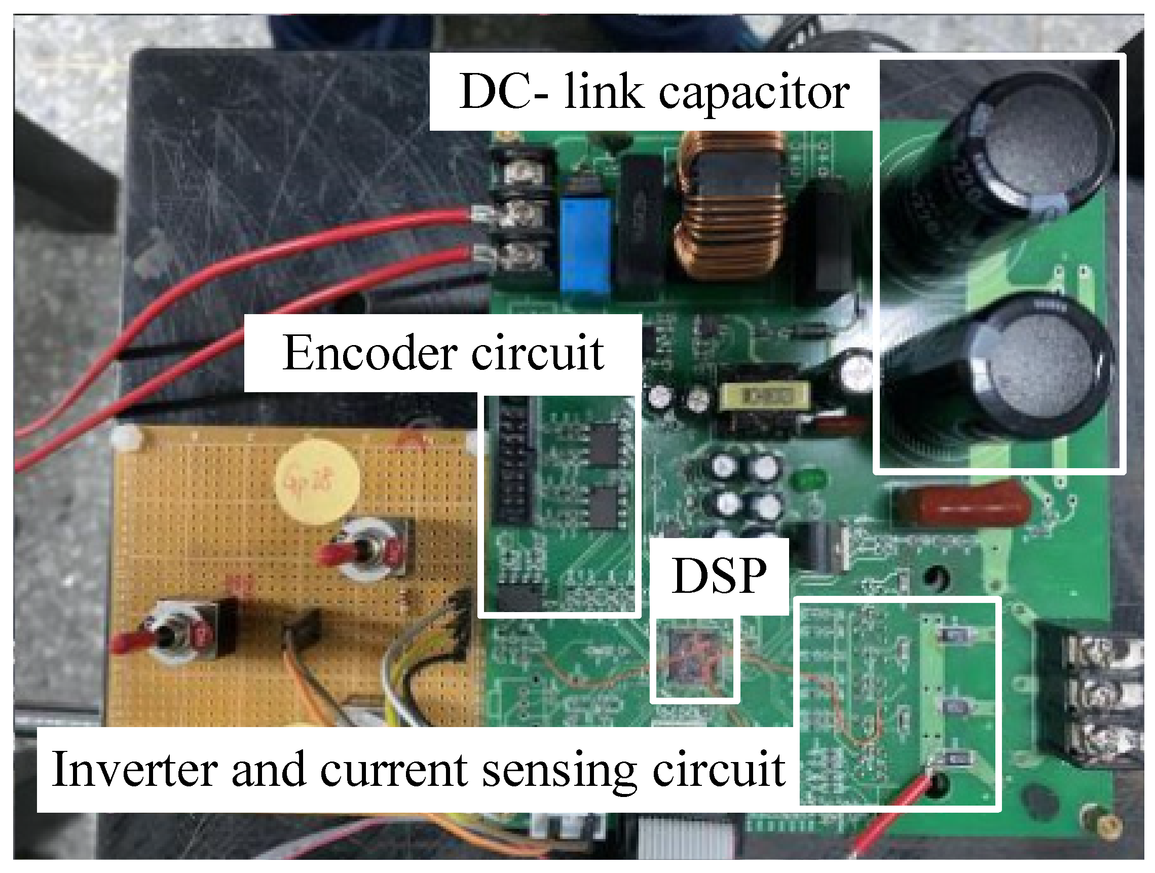
Figure 9a is a photograph of the SPMSM, including the stator, rotor, and air gap. The stator has 36 slots, a diameter of 150 mm, a 1 mm air-gap, and 3-phase distributed windings. The rotor has 12 poles with ferrite permanent-magnetic flanges. The diameter of the rotor is 220 mm, and a belt is attached to the rotor. Figure 9b is a photograph of the SPMSM drive system, including the encoder, the SPMSM, the mechanical coupling device, and the dynamometer. The encoder provides 2500 pulses/revolution. Figure 10 shows a photograph of the main circuit, including the inverter, sensing circuit, DSP, encoder circuit, and DC-link capacitor. The DSP is type TMS-320F-28035, manufactured by Texas Instruments. All of the circuits were designed and implemented by the authors of this paper.

Figure 9. Photographs of the SPMSM drive system. (a) motor (b) encoder, motor, and coupling connector.

Figure 10. Photograph of main circuits.

7. Experimental Results

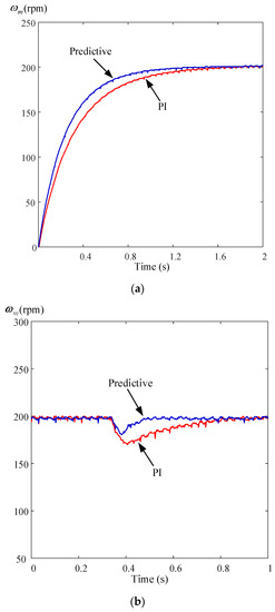
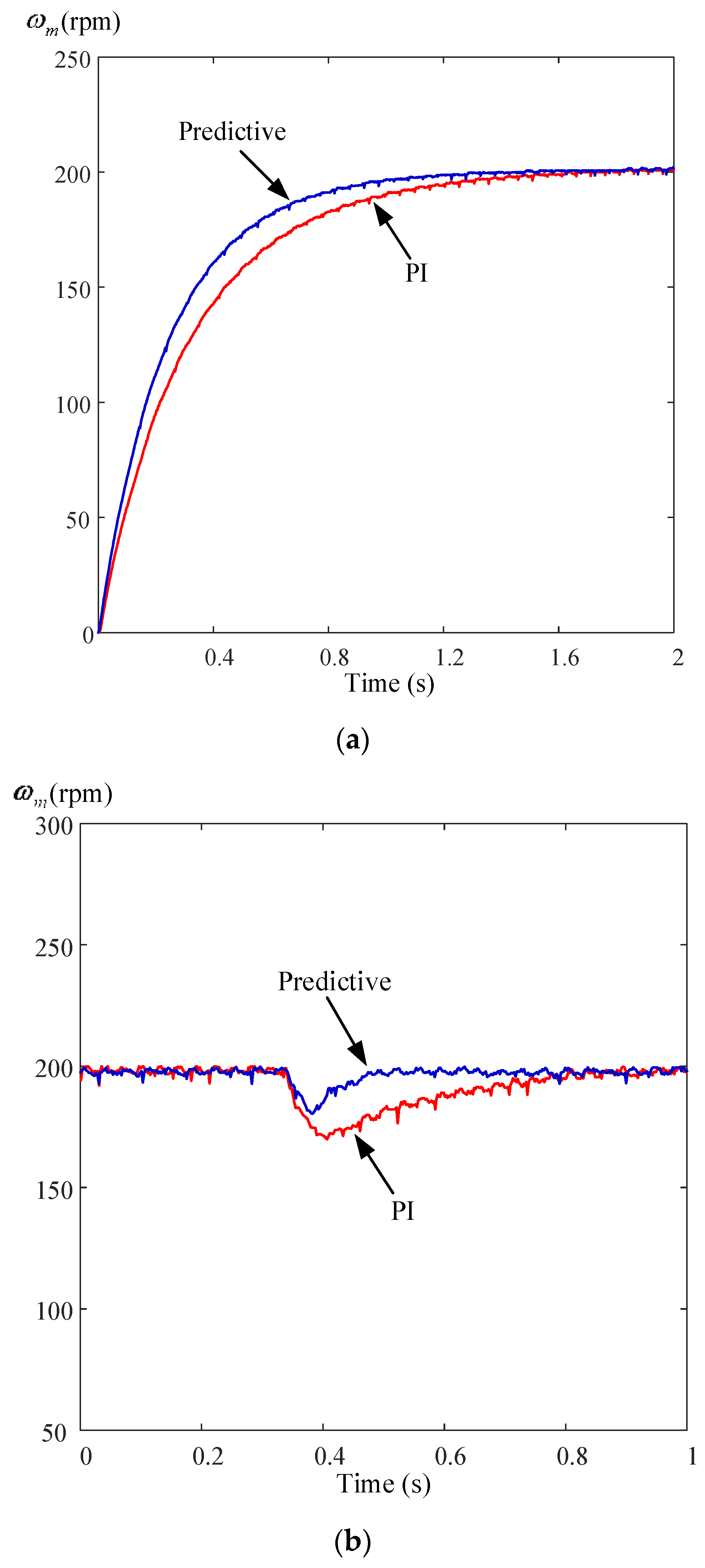
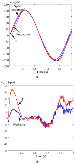
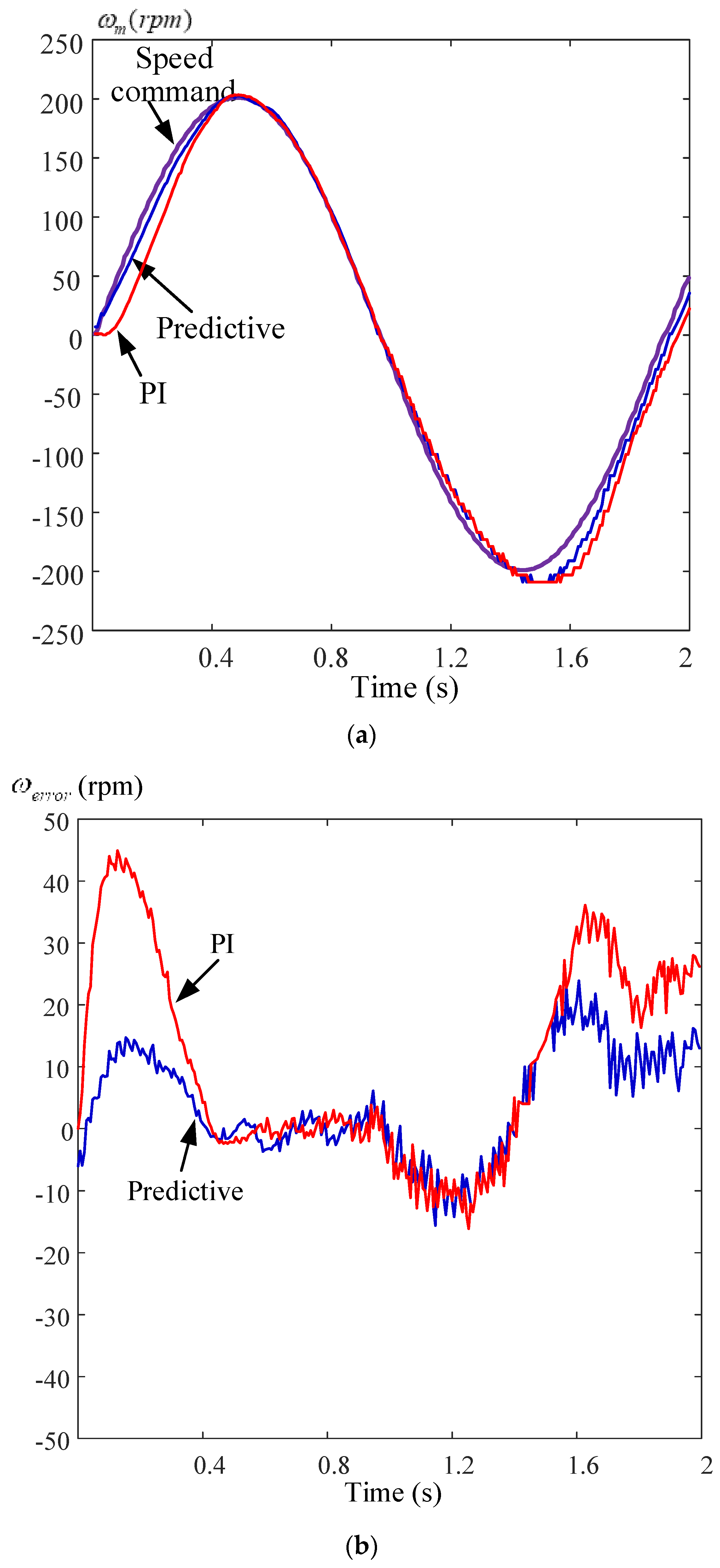
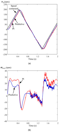
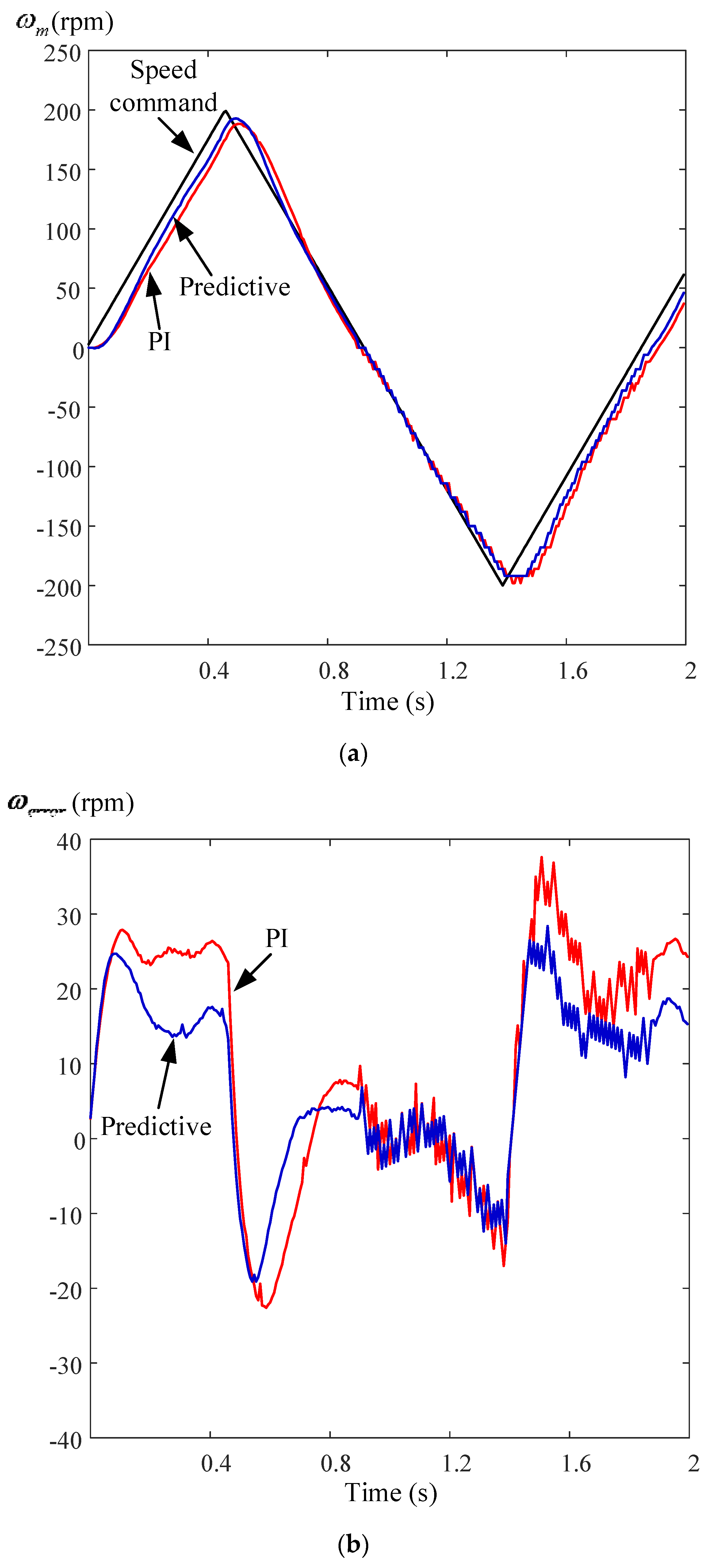
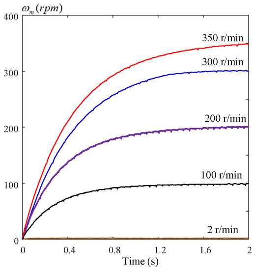
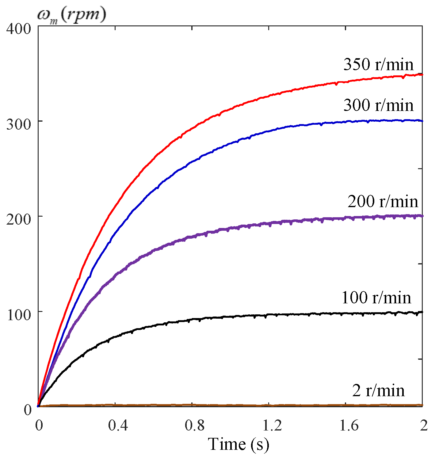
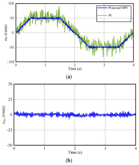
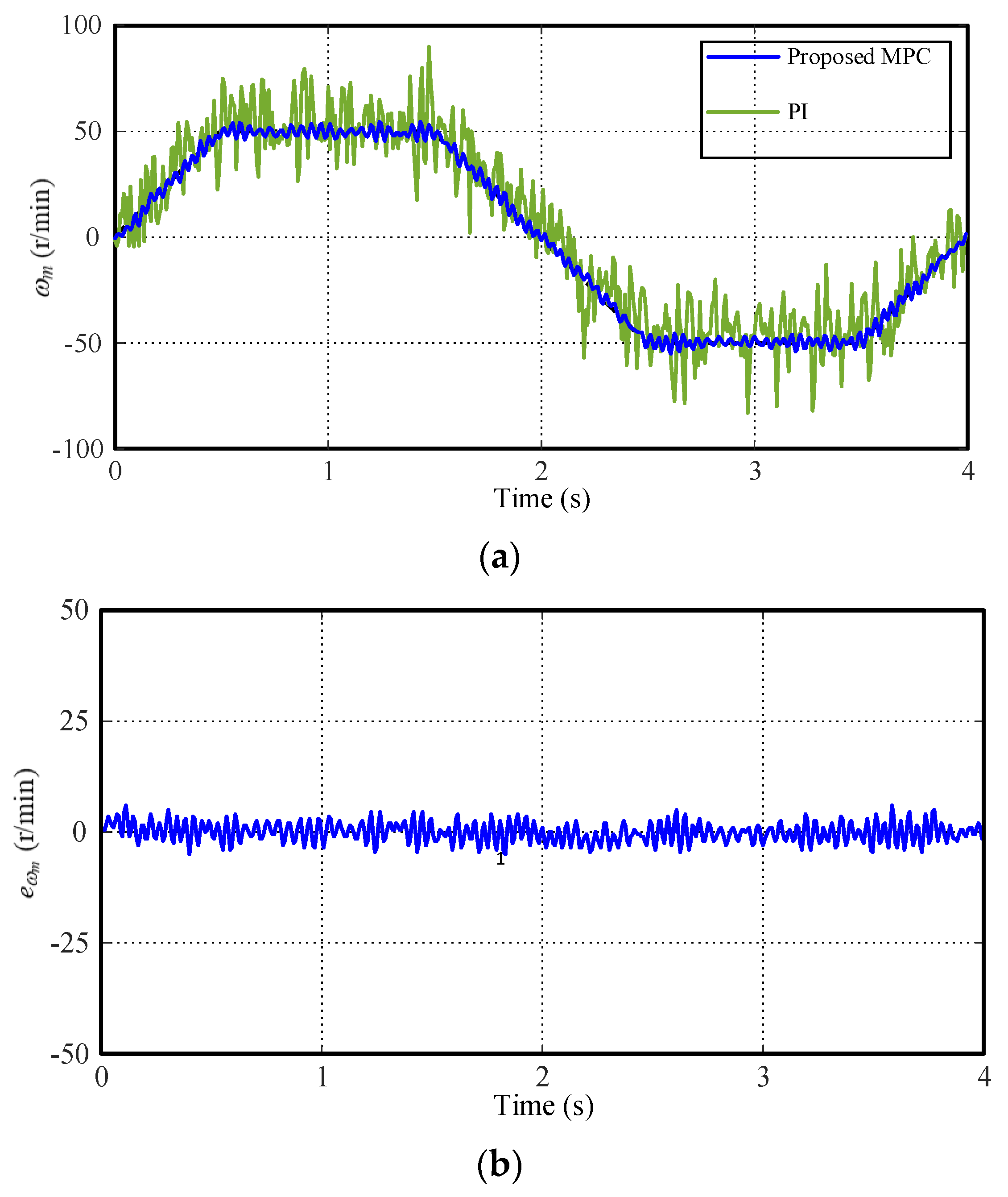
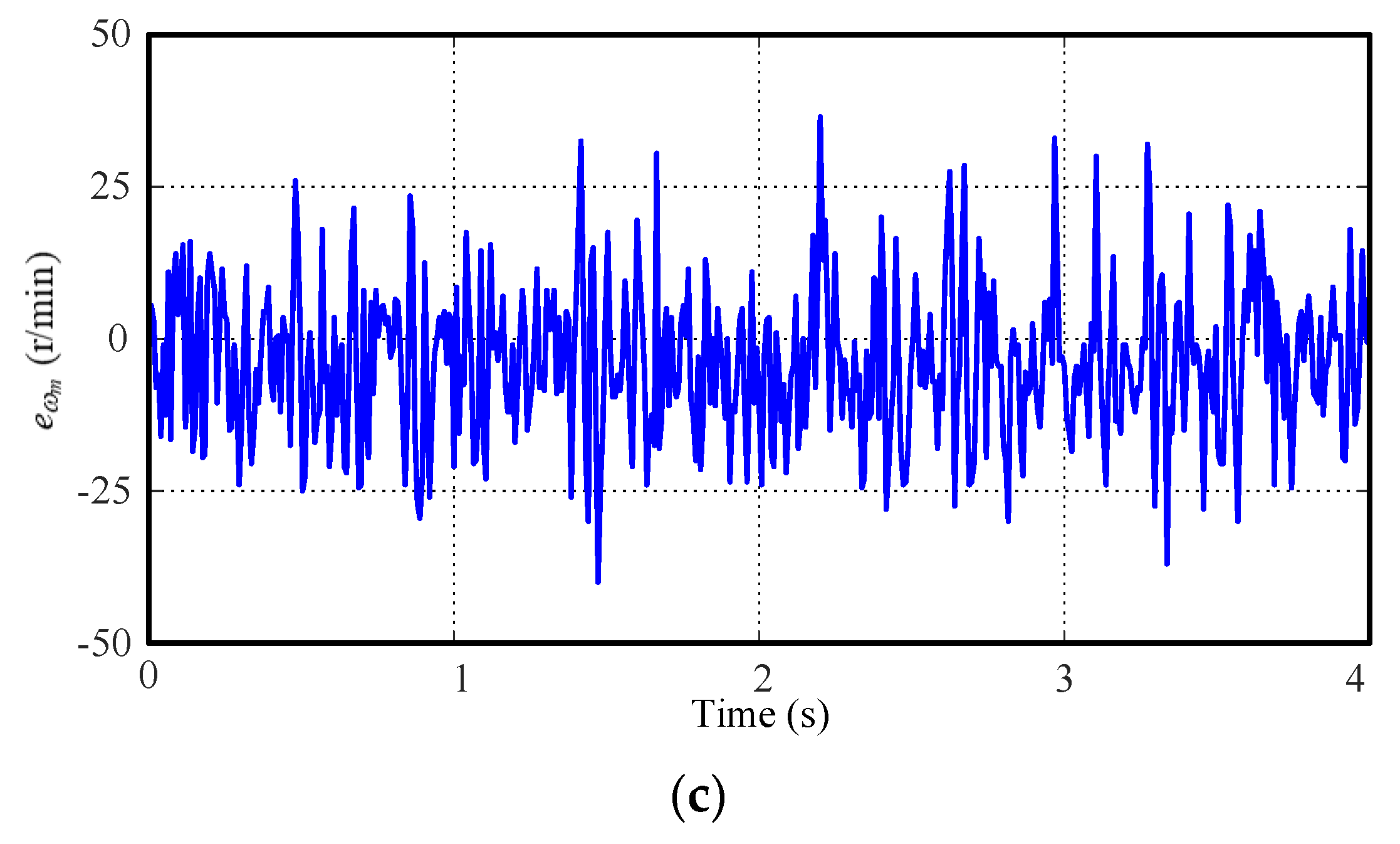
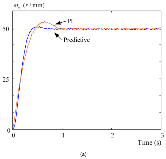
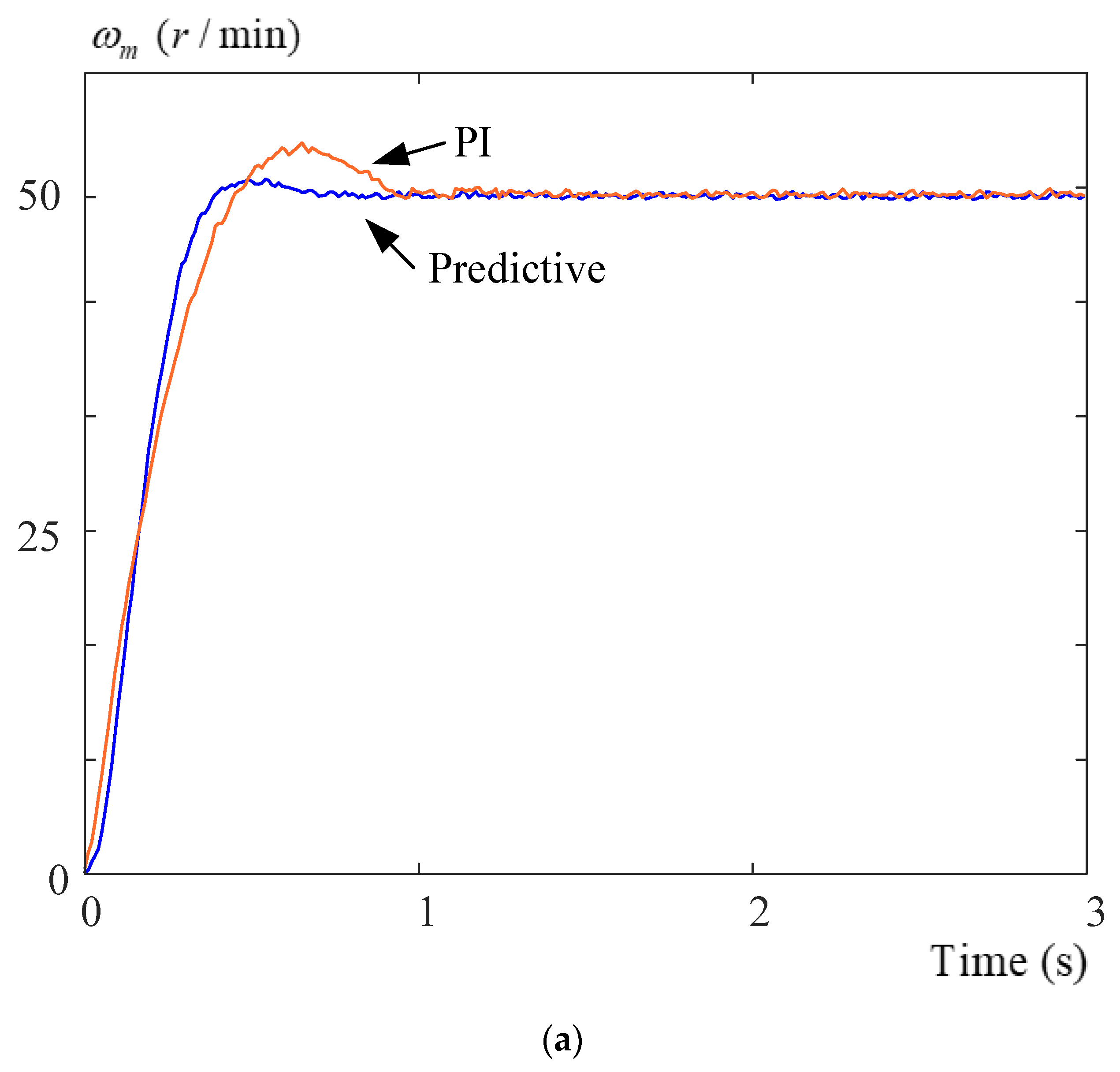
The experimental proto-type system in this paper uses a Texas Instruments DSP, type TMS-320-F-28035, as the control center. The measured execution time of the proposed predictive speed-loop control is 1 ms, and the measured execution time of the proposed predictive current-loop control is 100 µs. The input DC-link voltage is 24 V DC, which is provided by a DC power supply. The encoder is 2500 pulses/revolution. The dynamometer was manufactured by Chain-Tail Cooperation, type ZKB1S2AA, which uses a variable DC voltage to adjust the external load. The PMSM/PMSG was manufactured by Direction Technology and National Taiwan University of Science and Technology. To validate theoretical analysis, several experimental results are shown here. Figure 11a shows the measured speed responses at 200 r/min by using predictive controllers and PI controllers. Both of them have first-order transient responses because the SPMSM has an outer-rotor, which provides a great amount of inertia. As we can observe, the predictive controllers have faster transient responses than the PI controllers. Figure 11b shows the load disturbance responses under a 1 N·m load at 200 r/min. When an external load is added, the predictive controllers have a 20 r/min speed drop and a 0.2 s recovery time, but the PI controllers have a 40 r/min speed drop and a 0.5 s recovery time. Again, the predictive controllers have better performance than the PI controllers. Figure 12a shows the measured speed responses at a 200 r/min sinusoidal speed command. The predictive controllers have better performance, which can track the sinusoidal speed commands very well. The PI controllers, however, have a lag response due to the delay of the integrational controller. Figure 12b demonstrates the measured speed errors. The maximum tracking error of the predictive controllers is 12 r/min, but it is 45 r/min for the PI controllers. Figure 13a demonstrates the measured triangular speed responses at 200 r/min, and we can see that the predictive controllers have a faster tracking response than the PI controllers. Figure 13b demonstrates the measured speed errors under the same conditions. As we can observe, the maximum tracking error of the predictive controllers is 28 r/min, but it is 38 r/min for the PI controllers. Figure 14 displays the measured step-input transient responses at different commands from 2 r/min to 350 r/min when using the predictive controllers. All of the results have similar linear responses. As a result, it is not necessary to tune the parameters of the predictive controllers for different operating speeds.

Figure 11. Measured responses using different controllers. (a) transient, (b) load disturbance.

Figure 12. Measured sinusoidal responses using different controllers at 200 r/min. (a) speeds, (b) errors.

Figure 13. Measured triangular responses using different controllers at 200 r/min. (a) speeds, (b) errors.

Figure 14. Measured step-input speed responses at different commands.

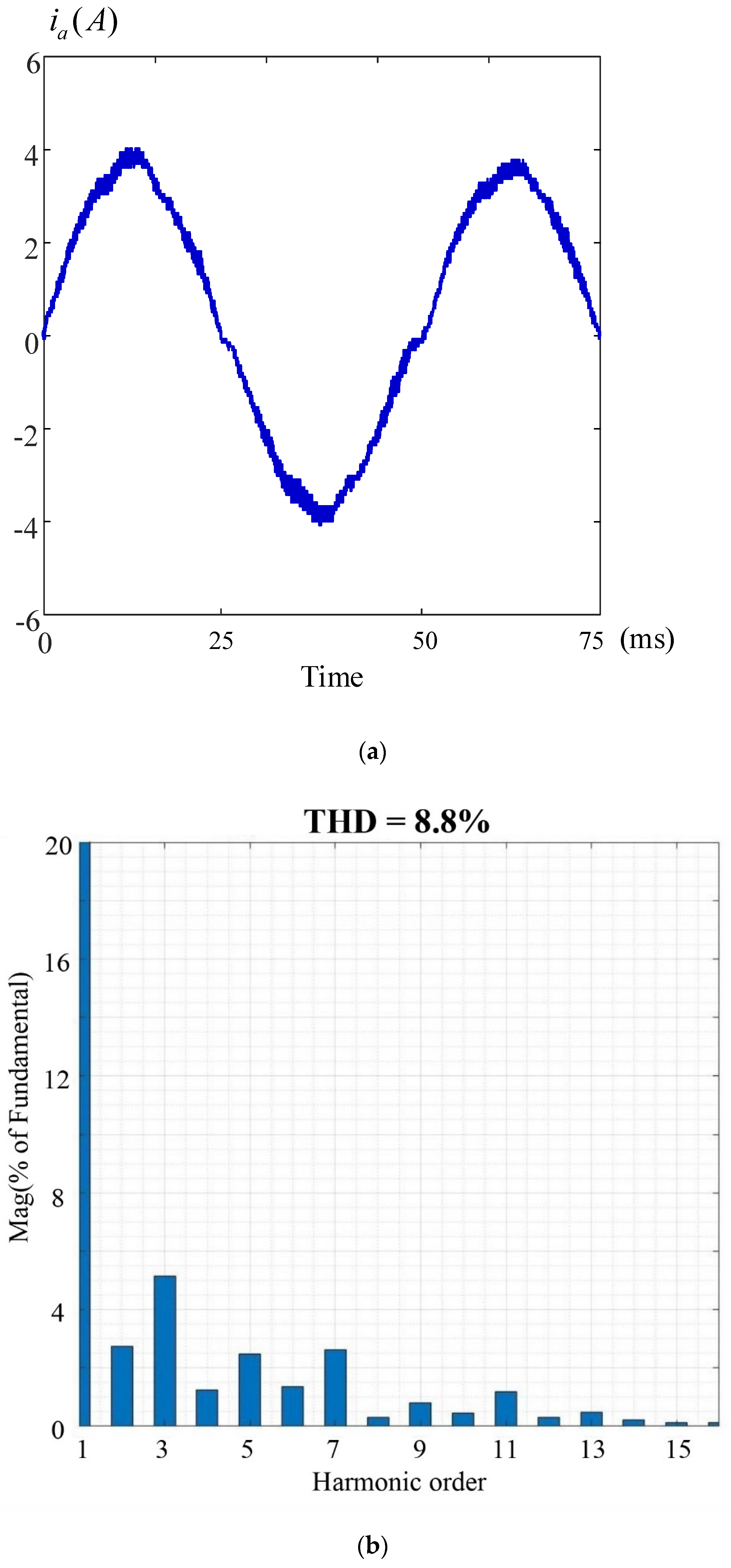
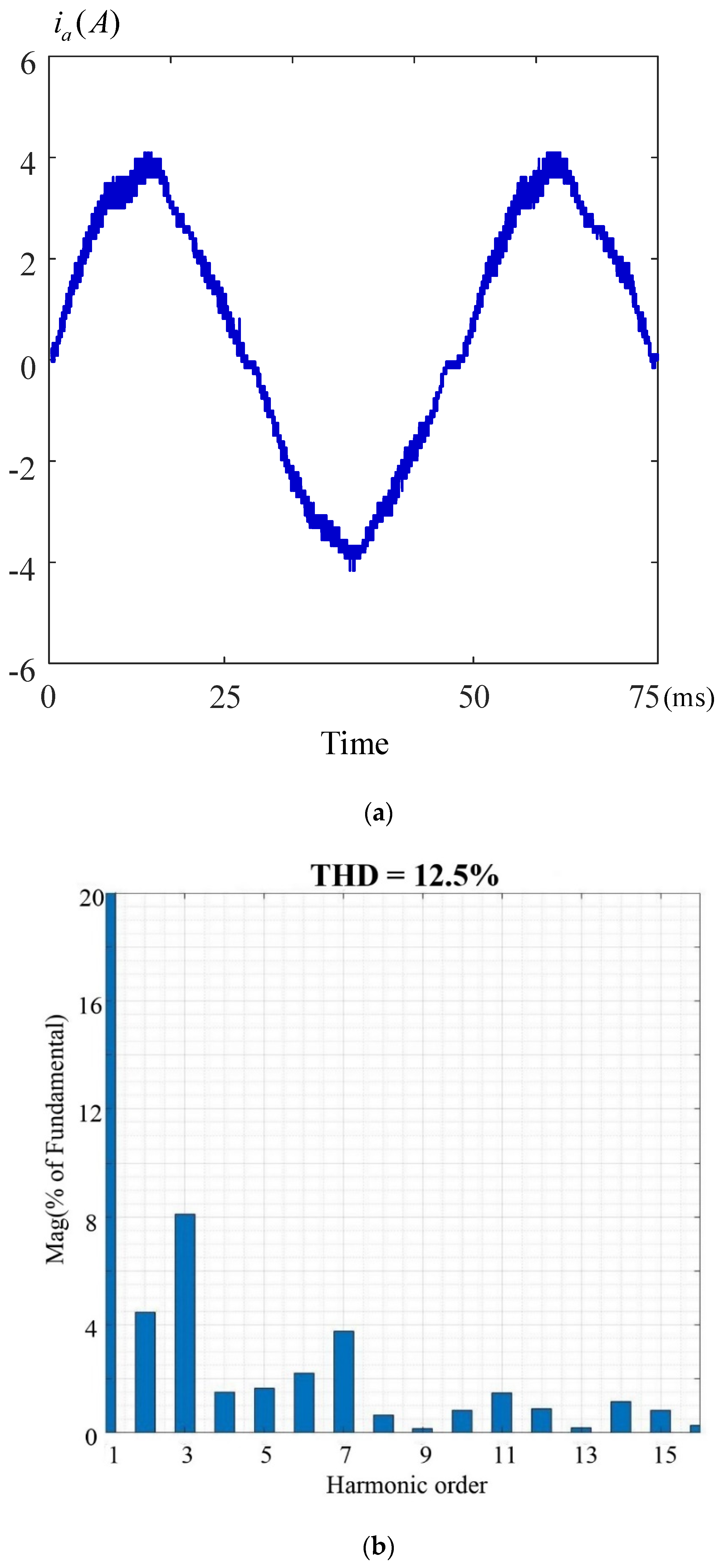
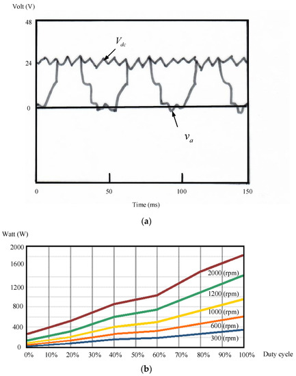
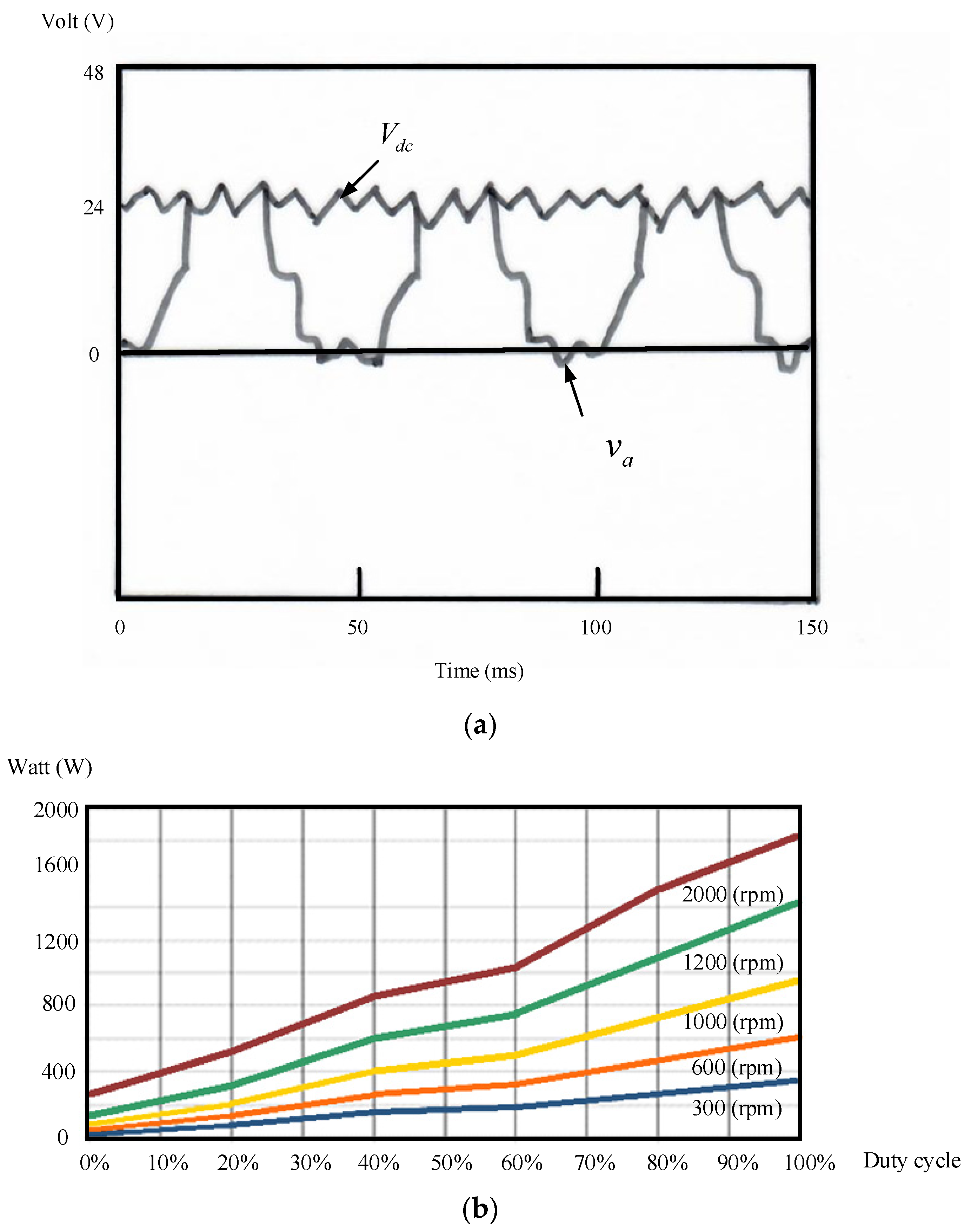
Figure 15a shows the measured a-phase current waveform at 200 r/min and 1 N·m by using a predictive current controller. Figure 15b demonstrates the harmonic spectrum from fundamental frequency up to the 15th harmonic by using the predictive current controller. We can see that the total harmonic distortion is 8.8%. Figure 16a shows the measured a-phase current waveform at 200 r/min and 1 N·m by using a PI current controller. Figure 16b demonstrates the harmonic spectrum by using the PI controller from the fundamental up to the 15th harmonic. We can see that the total harmonic distortion is 12.5%. Comparing Figure 15a,b and Figure 16a,b, we can conclude that the predictive current controller has better performance than the PI current controller. Figure 17a displays the measured voltage of the regenerative resistance load, which is used to charge the 24 V battery, and it also displays the a-phase voltage output that is generated by the SPMSG when the system is operated when regenerating energy. Figure 17b shows the measured regeneration voltage waveforms and power in Watts at different duty cycles of the buck converter with different speeds of the SPMPG.

Figure 15. Measured a-phase current using predictive controller. (a) waveform, (b) harmonics.

Figure 16. Measured a-phase current using PI controller. (a) waveform, (b) harmonics.

Figure 17. Measured regeneration voltage waveforms and power. (a) voltage waveforms, (b) power.

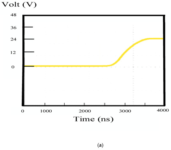
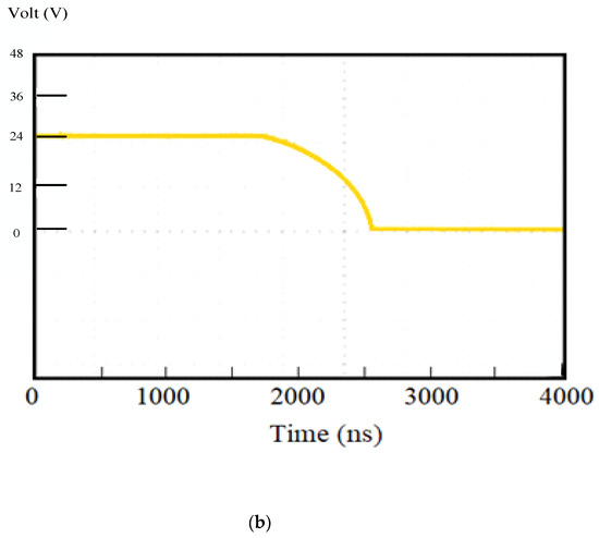
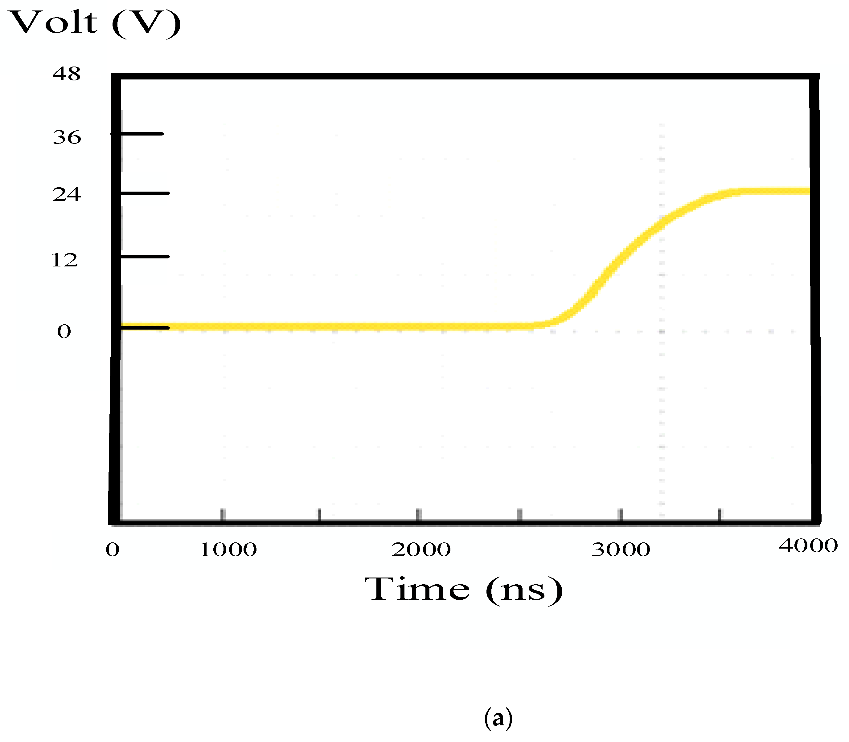
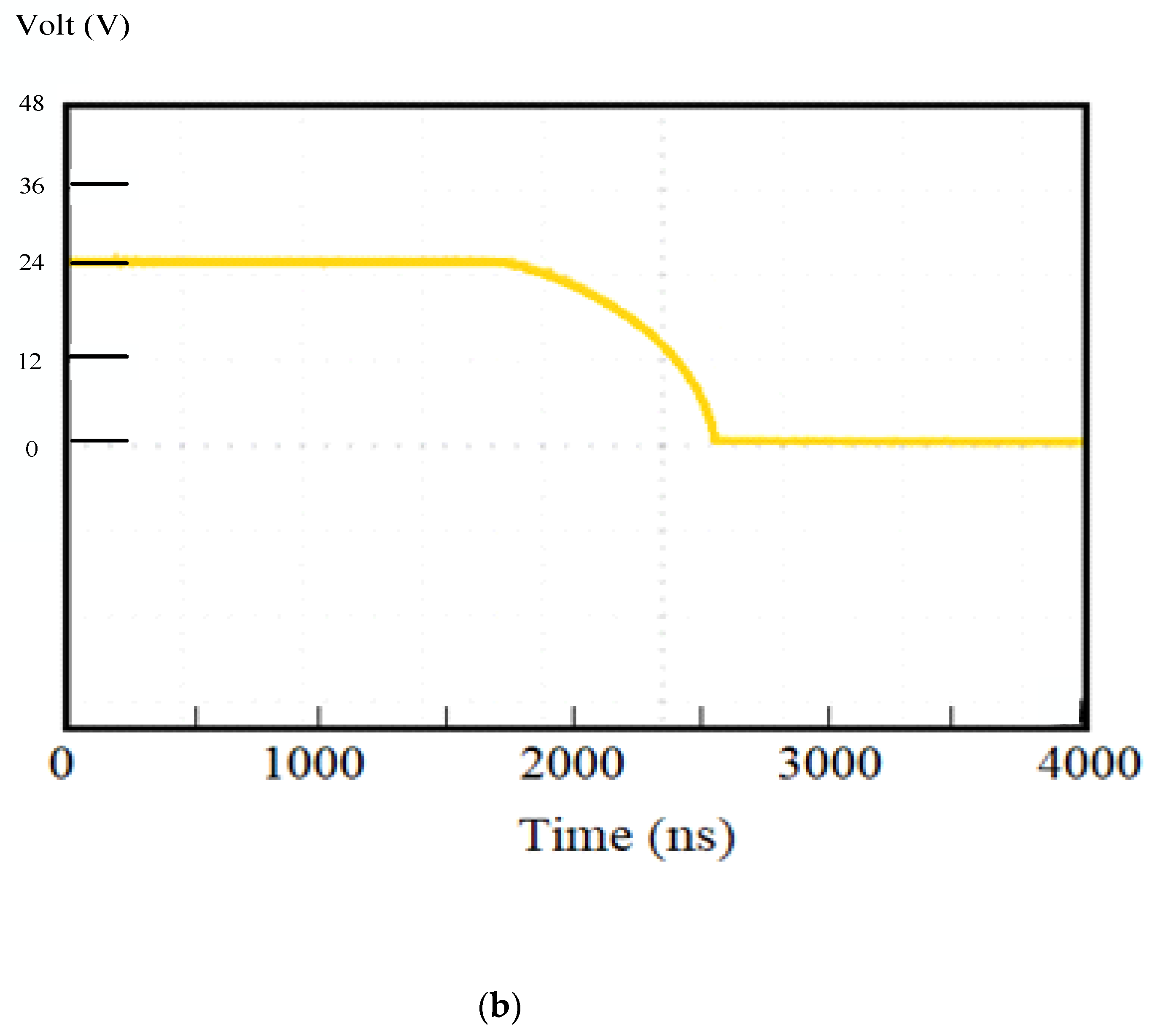
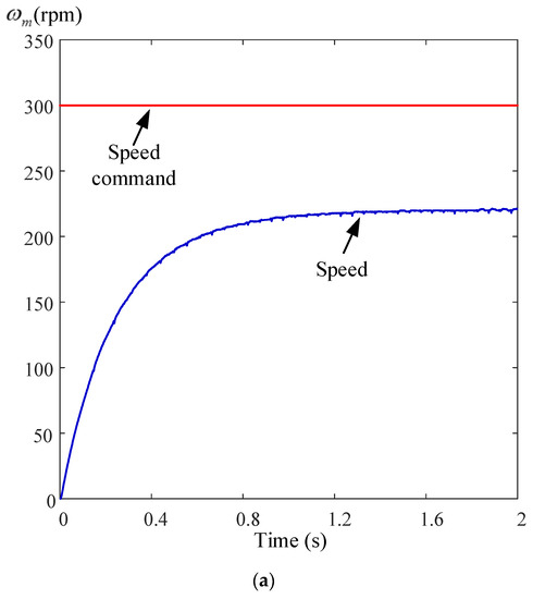
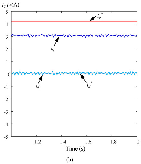
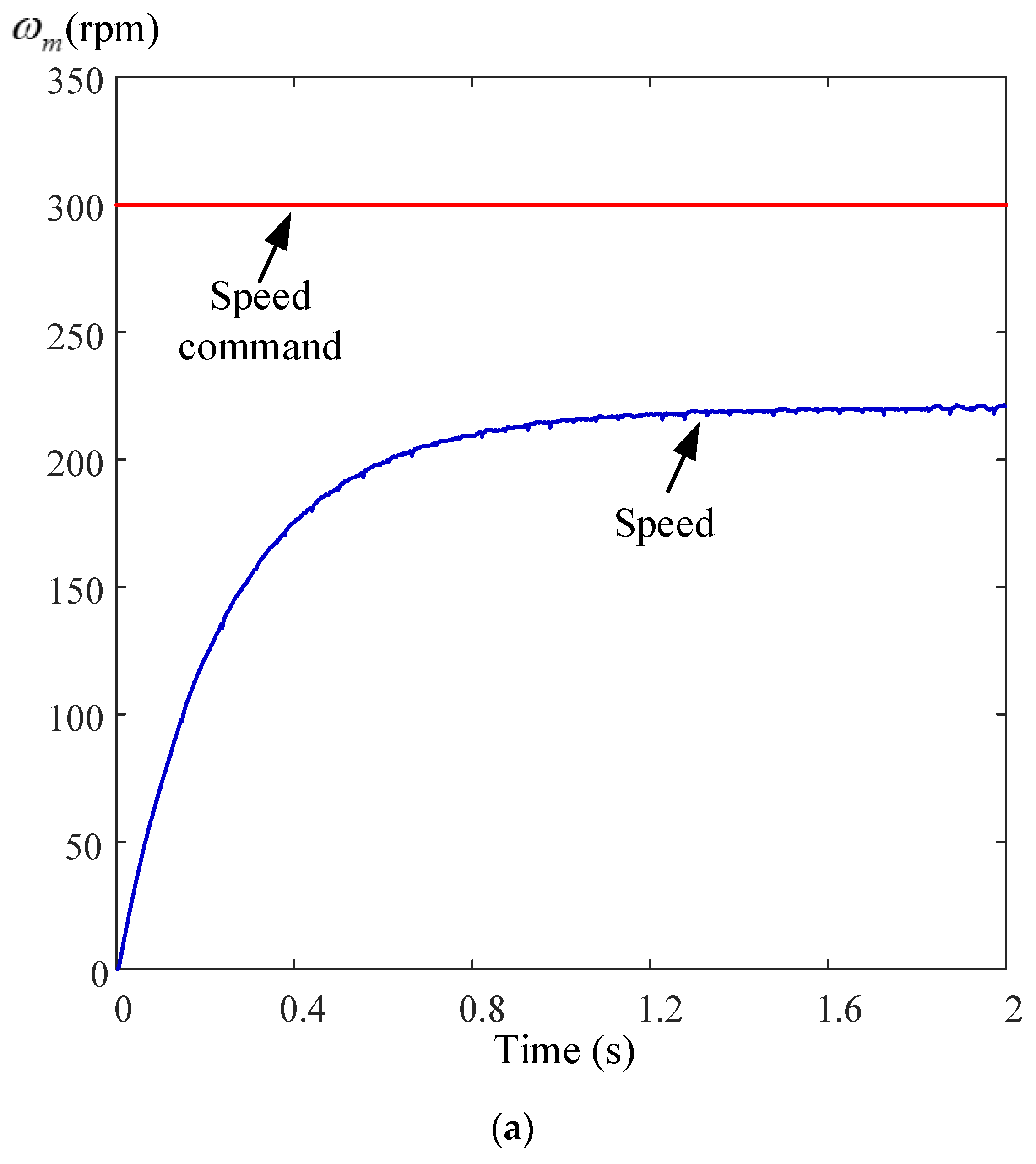
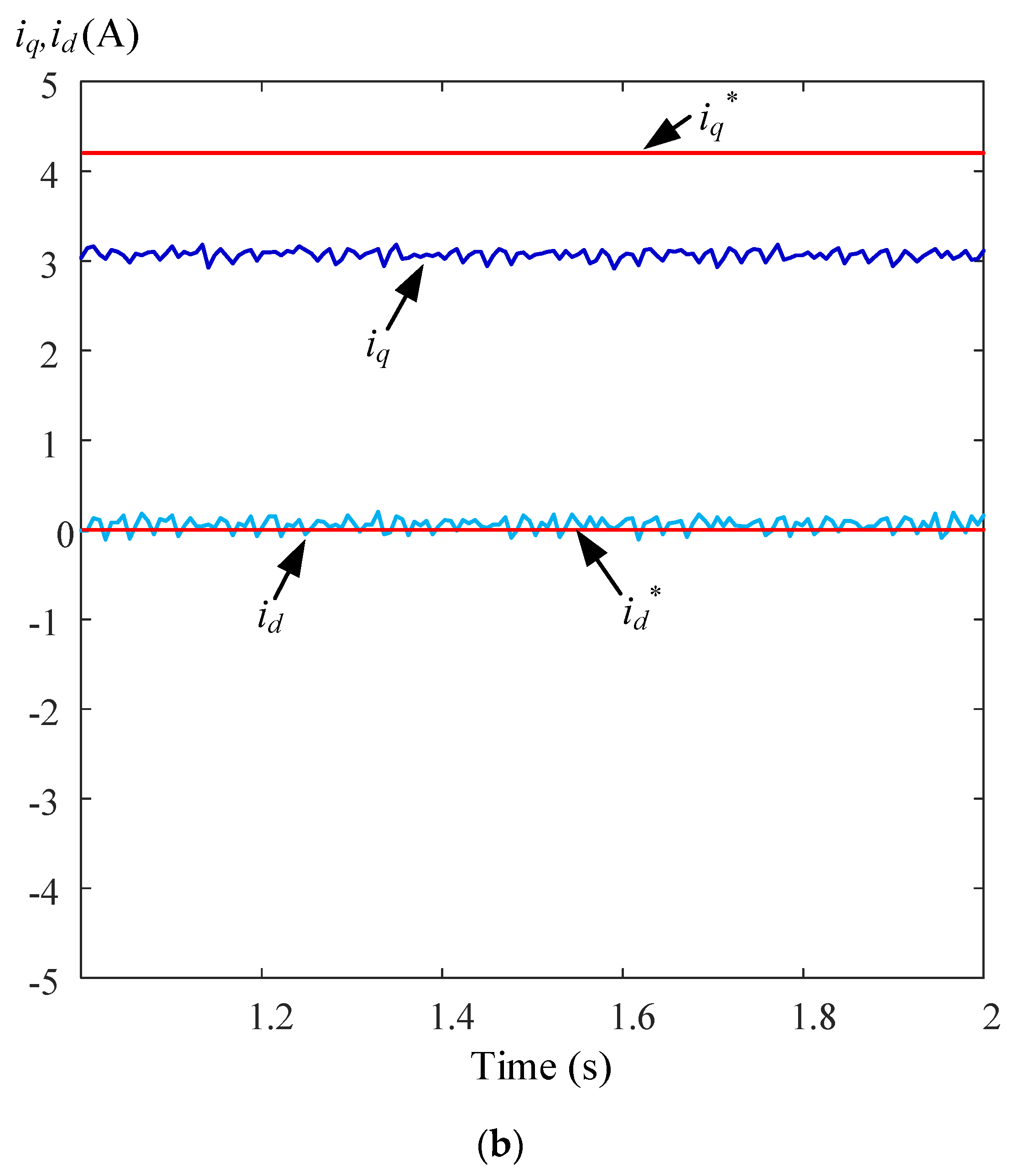
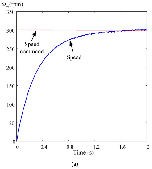
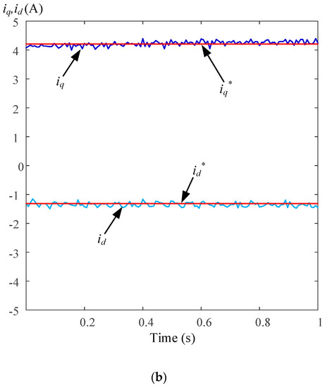
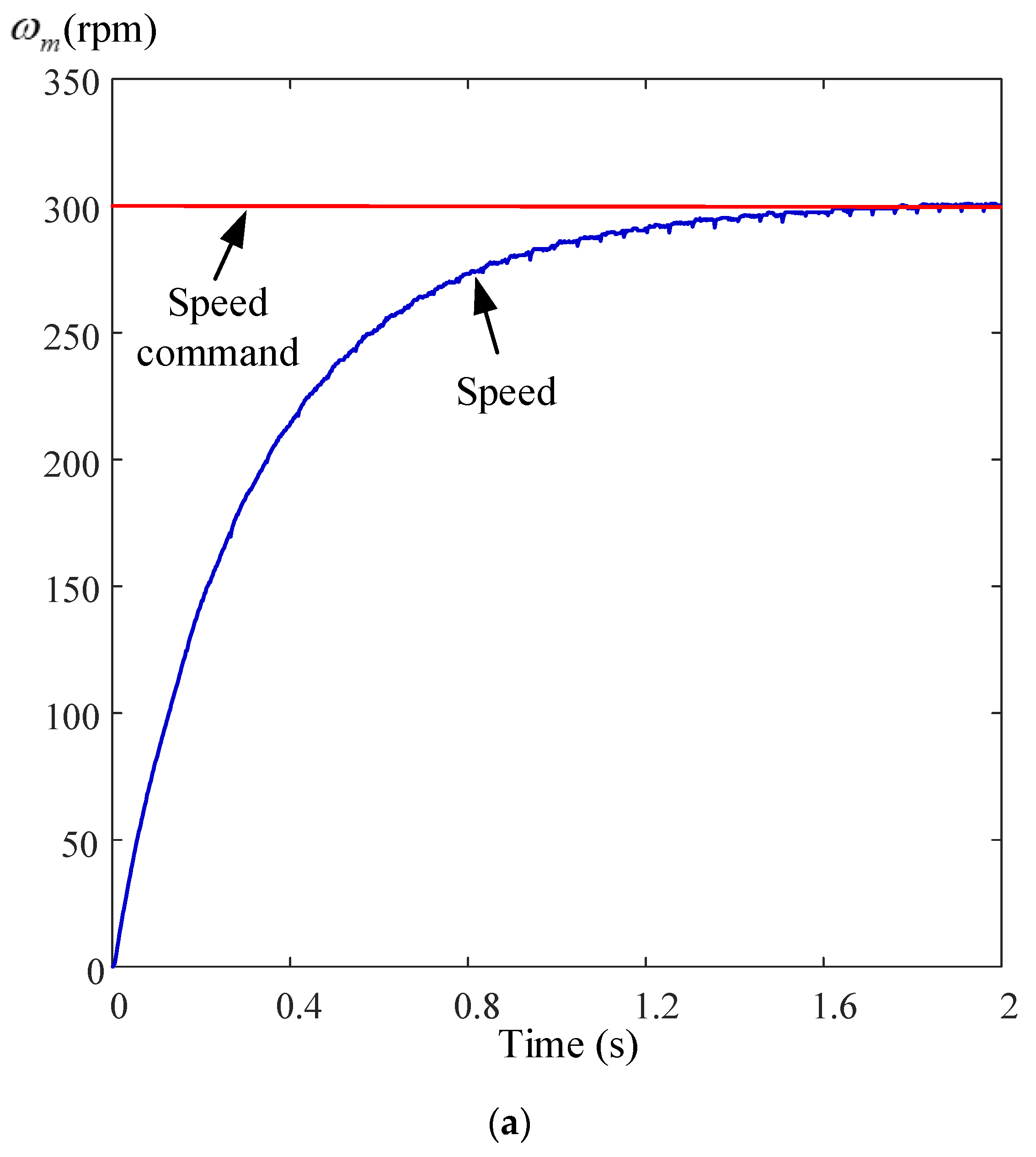
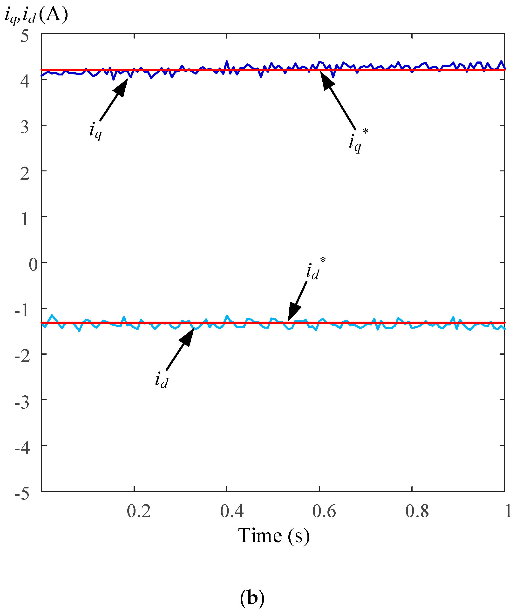
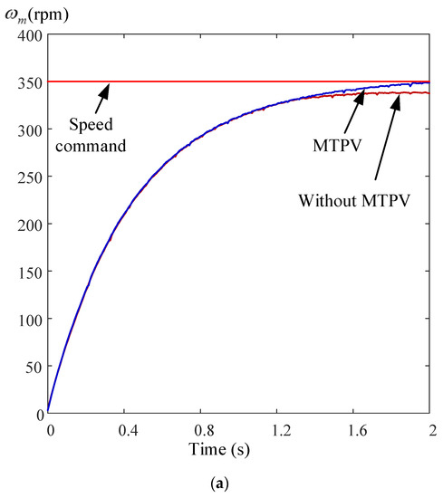
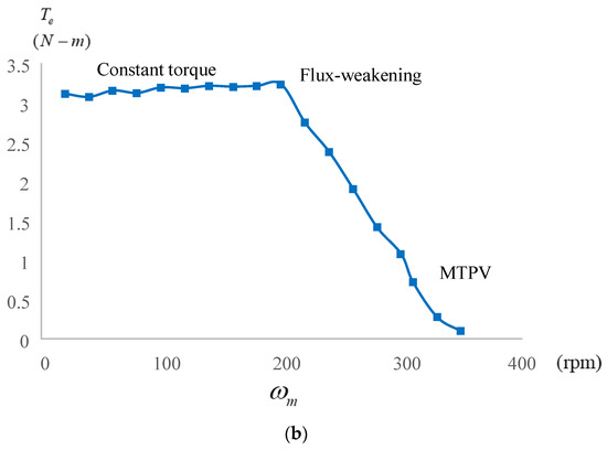
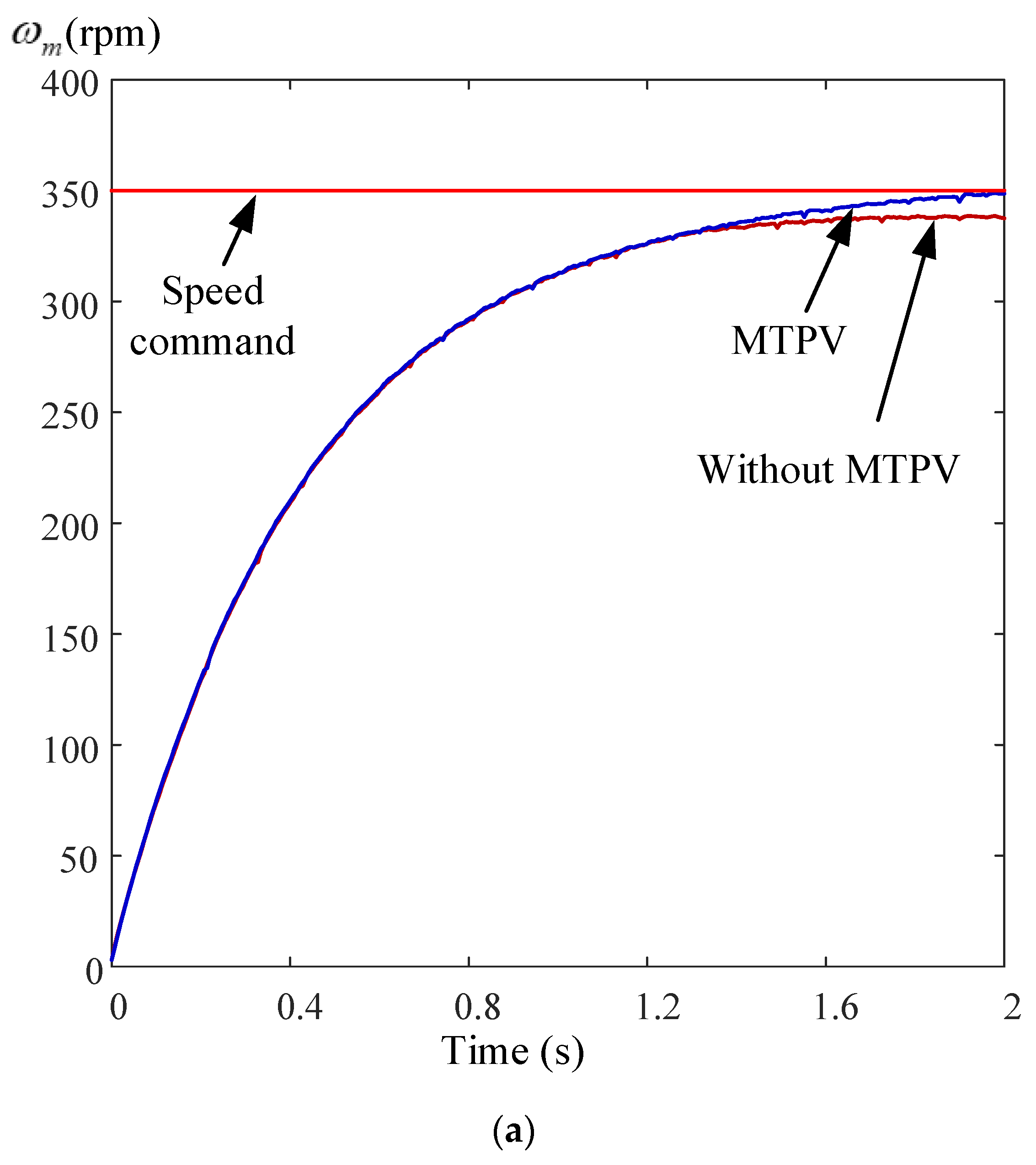
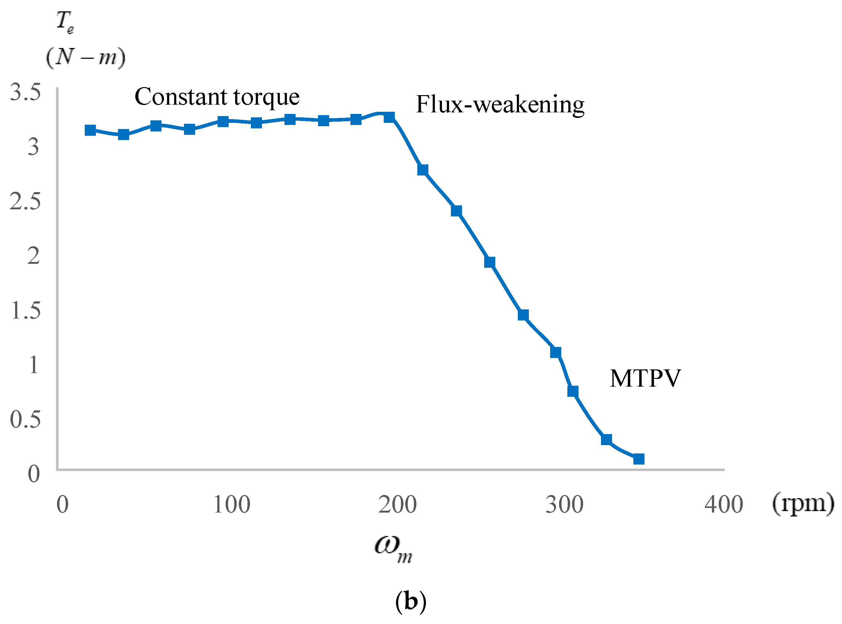
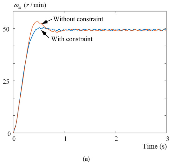
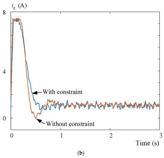
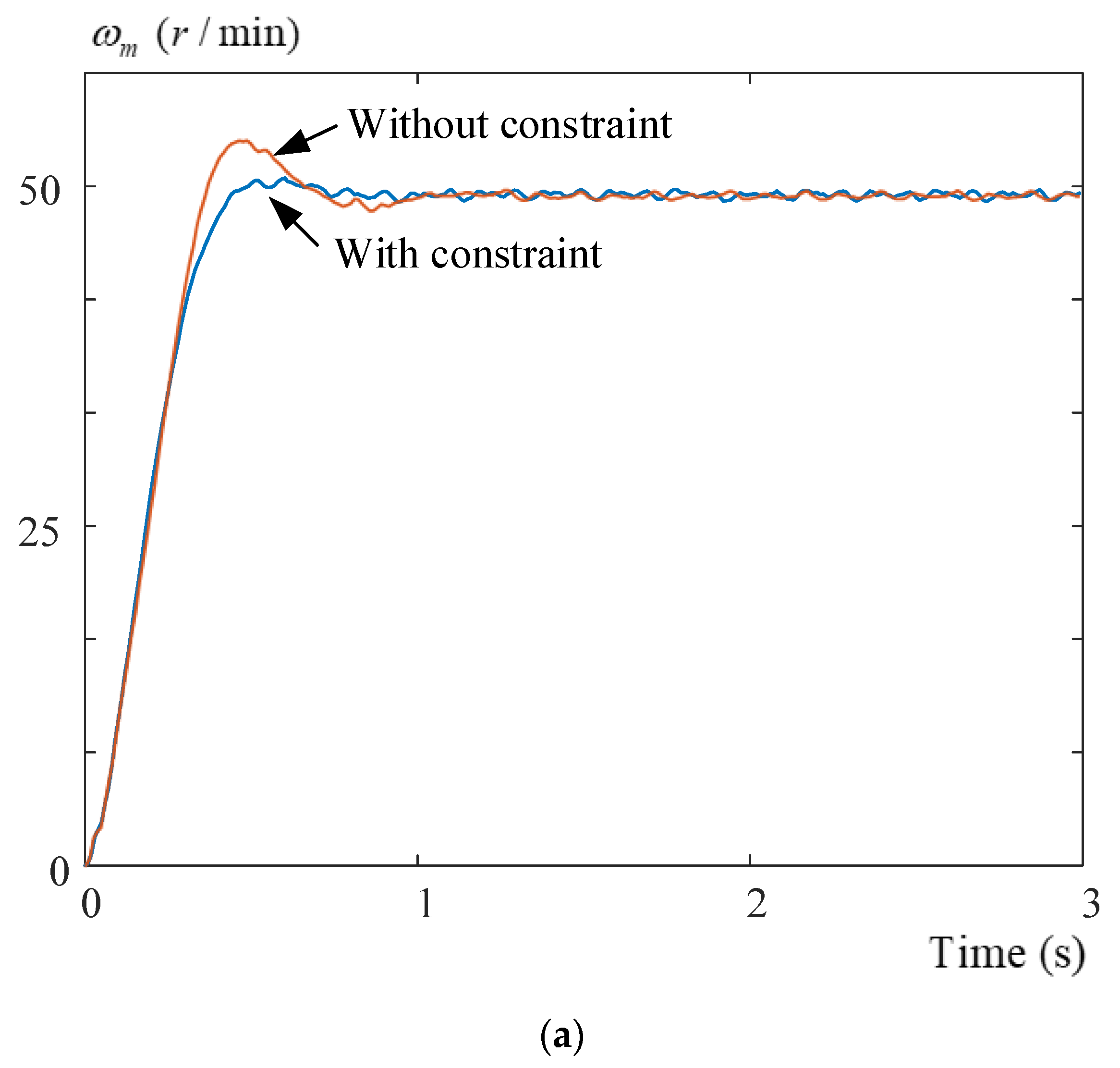
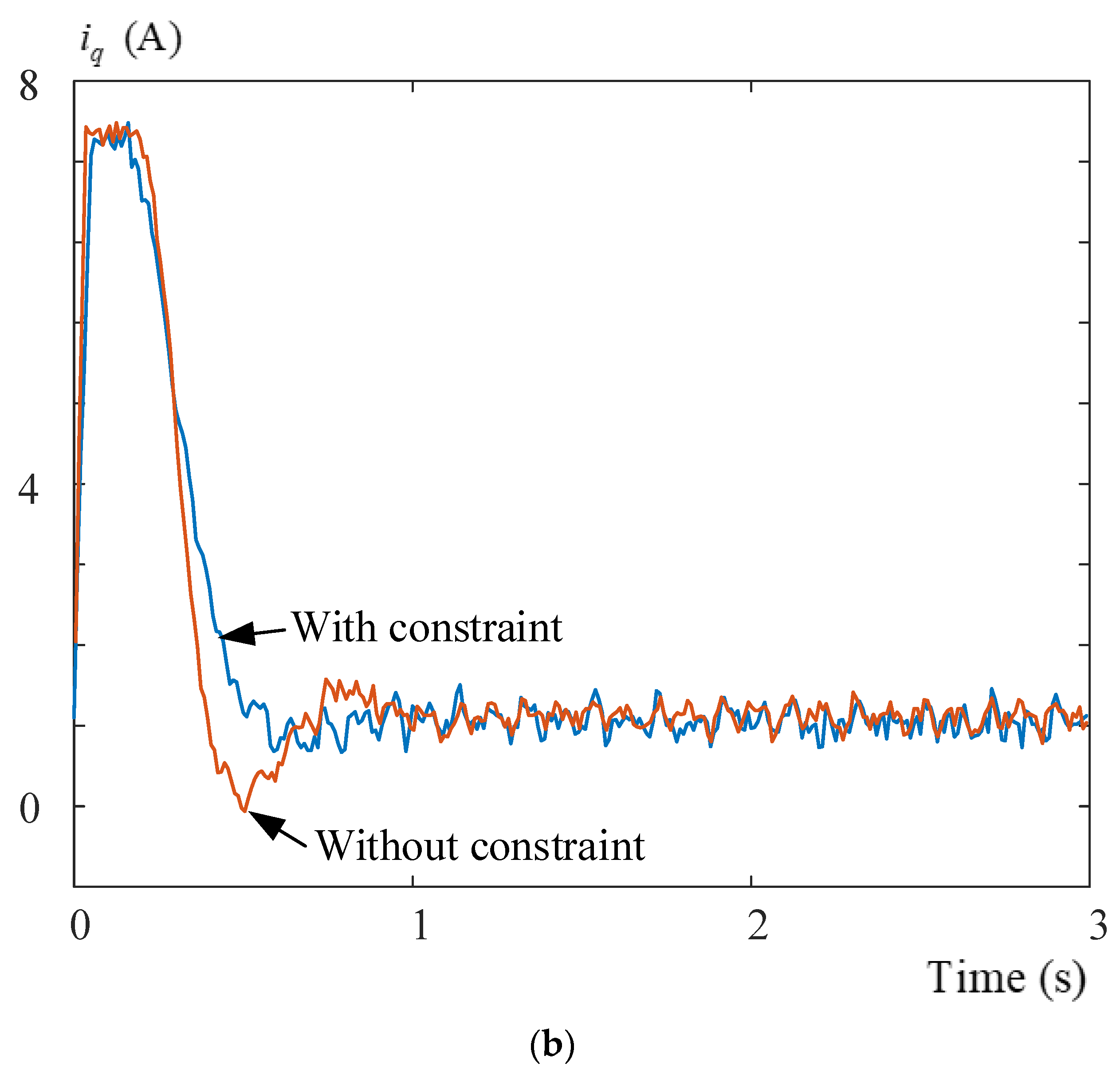
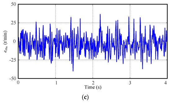
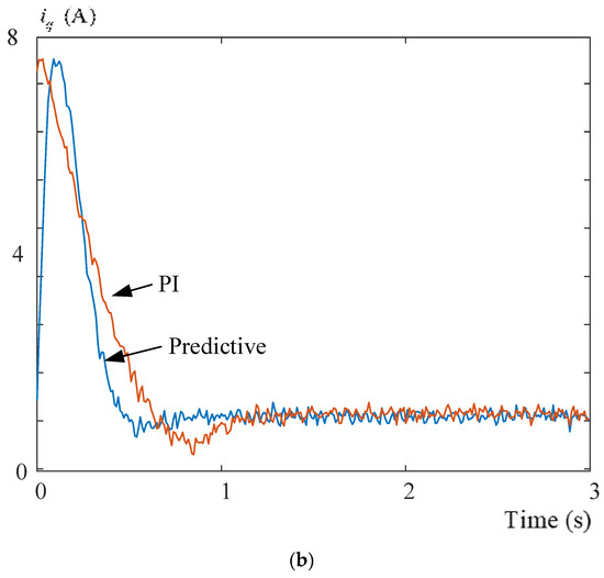
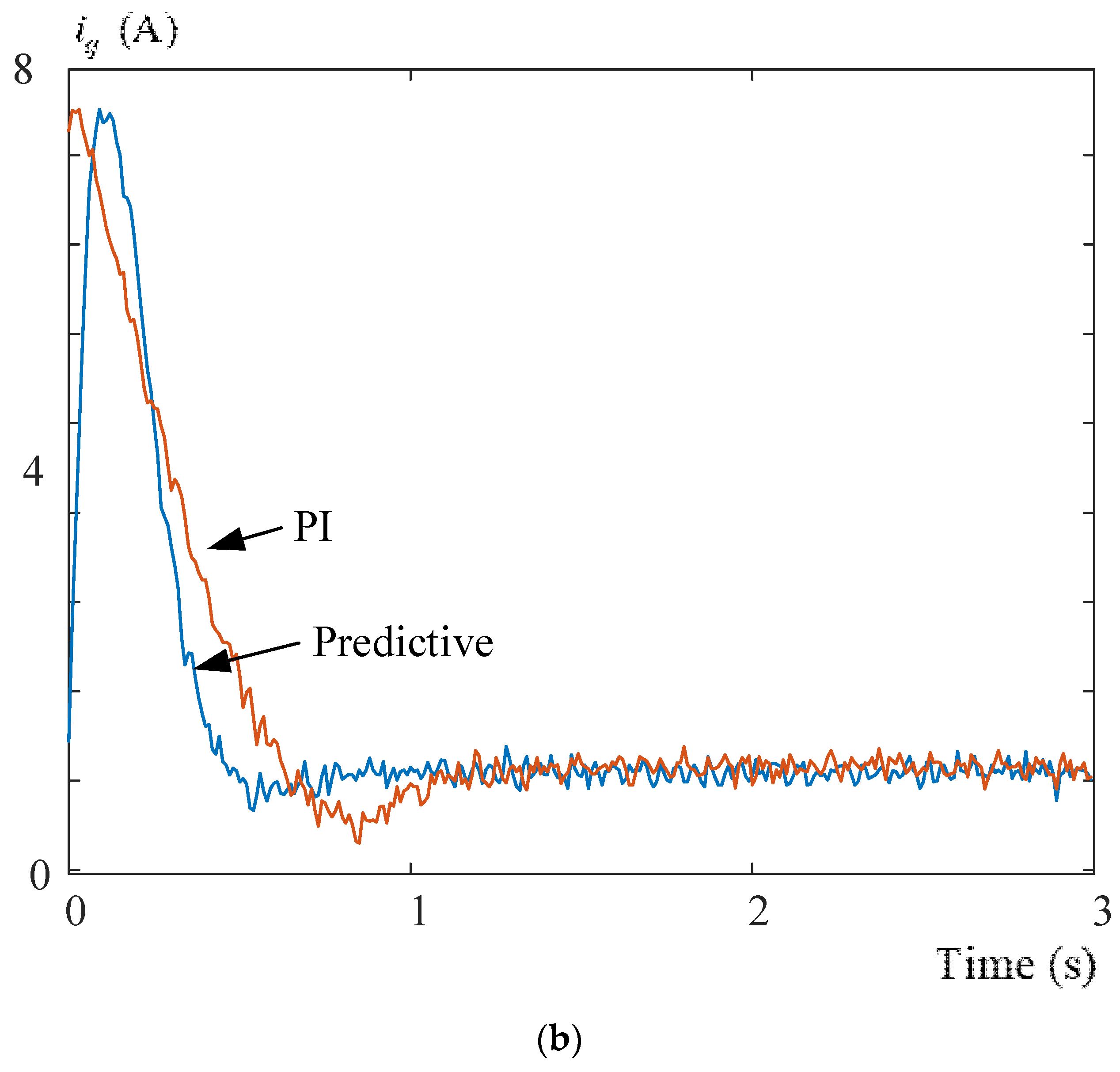
Figure 18a shows the measured voltage waveform when the relay is switched from “on” to “off”, and we can see that the switching interval is near 300 ns. Figure 18b shows the measured voltage waveform when the relay is switched from “off” to “on”, and the switching interval is near 900 ns. Figure 19a shows the measured speed responses without using the flux-weakening control. As we can observe, the speed cannot track the speed command because the back-EMF of the SPMSM is near 24 V. Figure 19b shows the related d-q axis current commands and their currents, and we see that the d-q currents cannot track their current commands. Figure 20a shows the measured speed responses at 300 r/min by using the flux-weakening control, and the measured speed can track the speed command well. Figure 20b shows the measured d-q axis commands and their measured d-q axis currents, and all of the d-q axis currents can track their current commands well. Figure 21a shows a comparison of the measured speed responses using and without using MTPV control. The adjustable speed range can be extended by using the proposed MTPV control. Figure 21b shows the measured torque-speed curve from 10 r/min to 350 r/min, including constant torque, flux-weakening, and maximum torque per volt regions. Figure 22a,b show the measured speed and current responses by using the new parameters of the predictive controllers with and without input current constraint. The responses using the input current constraint are smoother and slower than without using the input current constraint. Figure 23a–c show the measured responses when the motor parameters are varied. The predictive controller has better performance than the PI controller again. Figure 24a,b shows responses of the PI current controller and the new parameters of the predictive current controller. No torque sensor is used here. However, we can judge the torque ripples from the q-axis current ripples and speed ripples. As you can observe, from Figure 24a,b, the torque ripples between the predictive control and PI control are quite close. Therefore, we can conclude that the predictive controllers provide better transient responses but not better torque ripples than the PI controllers.

Figure 18. Measured voltage responses of relay. (a) off, (b) on.

Figure 19. Measured responses at 300 r/min without flux-weakening control. (a) speeds, (b) currents.

Figure 20. Measured responses at 300 r/min with flux-weakening control. (a) speeds, (b) currents.

Figure 21. Measured speed responses at 350 r/min with maximum torque/voltage control. (a) speeds, (b) torque-speed curve.

Figure 22. The measured responses at 50 r/min. (a) speeds, (b) currents.

Figure 23. Speed responses with varied parameters $2r_s$, $0.5L_d$, $0.5L_q$, and $2J$ at 50 r/min. (a) speeds. (b) proposed predictive controller. (c) PI errors.

Figure 24. Measured responses with different controllers. (a) speeds, (b) q-axis currents.

Table 1 shows the comparisons of the proposed predictive controllers and PI controllers that were designed by pole assignment method. As we can observe, the predictive controllers have better performance than the PI controllers, including faster rise time, shorter settling time, smaller steady-state errors, faster recovery times, smaller speed drops when an external load is added, and smaller tracking errors for both sinusoidal and triangular speed commands.

Table 1. Comparisons of predictive controllers and PI controllers.

Conditions	Specifications	PI Controllers	Predictive Controllers
200 r/min step-input command	Rise time	1 s	0.4 s
	Settling time	1.4 s	0.8 s
	Steady-state errors	±2 r/min	±1 r/min
200 r/min adding a 2N-m load	Recovery time	0.5 s	0.2 s
	Maximum speed drop	31 r/min	20 r/min
200 r/min sinusoidal speed command	Maximum speed error	44 r/min	22 r/min
	$\sqrt{\frac{{\displaystyle \sum _{k=1}^n{\omega }_{error}^2(k)}}{n}}$	194 r/min	94 r/min
200 r/min triangular speed command	Maximum speed error	37 r/min	28 r/min
	$\sqrt{\frac{{\displaystyle \sum _{k=1}^n{\omega }_{error}^2(k)}}{n}}$	188 r/min	134 r/min

8. Conclusions

In this paper, a 36-slot 12-pole outer-rotor SPMSM drive system with energy recovery is implemented. This new SPMSM/SPMSG system provides high torque and low-speed operating ranges, which are very suitable for indoor exercise bicycle applications. In addition, flux-weakening control and maximum torque per voltage control are proposed to easily extend its maximum motor speed to 1.75 times the rated speed. Moreover, the predictive-speed controller and predictive-current controller are designed and implemented to improve the transient responses, load disturbance responses, and tracking responses.

The paper proposes a new design method for a multi-pole outer-rotor SPMSM and its drive system which is very suitable for indoor exercise bicycle applications.

References

- Muetze, A.; Tan, Y.C. Electric bicycles. IEEE Ind. Appl. Maga. 2007, 13, 12–21. [Google Scholar] [CrossRef] [Scilit]
- Contò, C.; Bianchi, N. E-Bike Motor Drive: A Review of Configurations and Capabilities. Energies 2022, 16, 160. [Google Scholar] [CrossRef] [Scilit]
- Son, Y.-D.; Kang, G.-H. Drive System Design for a Permanent Magnet Motor with Independent Excitation Winding for an Electric Bicycle. J. Electr. Eng. Technol. 2010, 5, 623–630. [Google Scholar] [CrossRef] [Scilit]
- Misaki, C.; Hara, D.; Katayama, N.; Dowaki, K. Improvement of Power Capacity of Electric-Assisted Bicycles Using Fuel Cells with Metal Hydride. Energies 2020, 13, 6272. [Google Scholar] [CrossRef] [Scilit]
- Taha, H.M.; Alnaab, I. Designs of PMSMs with Inner and Outer Rotors for Electric Bicycle Applications. Kurd. J. Appl. Res. 2019, 4, 20–25. [Google Scholar] [CrossRef] [Scilit]
- Zhang, P.; Zhang, Q. A controller of PMSM for electrical bicycle with Hall effect sensors. In Proceedings of the 2016 IEEE 11th Conference on Industrial Electronics and Applications (ICIEA), Hefei, China, 5–7 June 2016; pp. 619–623. [Google Scholar]
- Park, S.-Z.; Kim, Y.-K.; Song, C.-H.; Lee, J.-W.; Mok, H.-S. Operation method of electric bicycle using change of BLDC operation mode and PMSM operation mode. In Proceedings of the 8th International Conference on Power Electronics—ECCE Asia, Jeju, Republic of Korea, 30 May 2011–3 June 2011; pp. 2529–2536. [Google Scholar] [CrossRef] [Scilit]
- Hammoud, I.; Hentzelt, S.; Xu, K.; Oehlschlagel, T.; Abdelrahem, M.; Hackl, C.; Kennel, R. On Continuous-Set Model Predictive Control of Permanent Magnet Synchronous Machines. IEEE Trans. Power Electron. 2022, 37, 10360–10371. [Google Scholar] [CrossRef] [Scilit]
- Eldeeb, H.; Hackl, C.M.; Horlbeck, L.; Kullick, J. A unified theory for optimal feedforward torque control of anisotropic synchronous machines. Int. J. Control. 2017, 91, 2273–2302. [Google Scholar] [CrossRef] [Scilit]
- Hammoud, I.; Xu, K.; Hentzelt, S.; Oehlschlaegel, T.; Kennel, R. On Offset-Free Continuous Model Predictive Current Control of Permanent Magnet Synchronous Motors. IFAC-PapersOnLine 2020, 53, 6662–6669. [Google Scholar] [CrossRef] [Scilit]
- Xu, H.; Gui, X.; Luan, T.; Lang, X.; Xu, D. A robust predictive current controller with incremental model and inductance observer for PMSM drive. In Proceedings of the 2017 IEEE Transportation Electrification Conference and Expo, Asia-Pacific (ITEC Asia-Pacific), Harbin, China, 7–10 August 2017; pp. 1–6. [Google Scholar] [CrossRef] [Scilit]
- Asp, K. What You Should Know about Buying an Exercise Bike and These 5 Other Home Gym Picks. Everyday Health. 1 April 2019. Available online: https://www.wikihow.com (accessed on 17 February 2023).
- Sul, S.-K. Control of Electric Machine Drive Systems; John Wiley & Sons: Hoboken, NJ, USA, 2011. [Google Scholar] [CrossRef] [Scilit]
- Krishnan, V.; Pasqualetti, F. On direct vs indirect data-driven predictive control. In Proceedings of the 2021 60th IEEE Conference on Decision and Control (CDC), Austin, TX, USA, 1 February 2022; pp. 736–741. [Google Scholar]
- Khaled, N.; Pattel, B. Practical Design and Application of Model Predictive Control; Elsevier: Oxford, UK, 2018. [Google Scholar]
- Xi, Y.; Li, D. Predictive Control-Fundamentals and Developments; Wiley: Singapore, 2019. [Google Scholar]
- Rodriquez, J.; Cortes, P. Predictive Control of Power Converters and Electrical Drives; Wiley and IEEE Press: West Sussex, UK, 2012. [Google Scholar]
- Wang, L. Model Predictive Control System Design and Implementation Using MATLAB; Spinger: London, UK, 2009. [Google Scholar]
- Bose, B.K. Modern Power Electronics and AC Drives; Prentice Hall: New York, NY, USA, 2001. [Google Scholar]
Disclaimer/Publisher’s Note: The statements, opinions and data contained in all publications are solely those of the individual author(s) and contributor(s) and not of MDPI and/or the editor(s). MDPI and/or the editor(s) disclaim responsibility for any injury to people or property resulting from any ideas, methods, instructions or products referred to in the content. |
© 2023 by the authors. Licensee MDPI, Basel, Switzerland. This article is an open access article distributed under the terms and conditions of the Creative Commons Attribution (CC BY) license (https://creativecommons.org/licenses/by/4.0/).