Time Estimation Algorithm of Single-Phase-to-Ground Fault Based on Two-Step Dimensionality Reduction

Abstract

The fault detection time identified by relying on the over-voltage criterion of zero-sequence voltage often lags behind the actual occurrence time of ground faults, which may cause fault protection methods based on transient quantity principles to miss fault characteristics and lose their protection capability. To accurately estimate the time of occurrence of a single-phase-to-ground fault, this paper proposes a two-step dimensionality reduction algorithm for estimating the time of occurrence of a single-phase-to-ground fault in a distribution network. This algorithm constructs a filter based on Empirical Mode Decomposition (EMD) to establish a high-dimensional feature dataset based on the zero-sequence current of all feeders. After Principal Component Analysis and Hilbert Mapping Algorithm, the high-dimensional data are reduced to two dimensions to construct a two-dimensional feature dataset. The density-based clustering method is used to adaptively divide the data into two categories, fault data and non-fault data, so as to estimate the time of occurrence of the fault. The paper designs 11 sets of experiments including 7 common high-resistance grounding mediums to verify the accuracy of the fault time recognition of this algorithm. The accuracy of this algorithm is within 7.3 ms and it exhibits better detection performance compared to the threshold detection method.

1. Introduction

The probability of single-phase-to-ground faults in power distribution networks is high, which is the main factor leading to forest fires and casualties from electric shocks [1]. We need to quickly determine the occurrence time of a single-phase-to-ground fault, which is mainly due to two factors. On the one hand, although a single-phase-to-ground fault in a distribution system can operate for an extended period, but the presence of an arc at the fault location may gradually expand over time, increasing the risk. “The Technical Guidelines for Power Distribution Networks” issued by the State Grid Corporation of China puts forward the principle of “instantaneous fault arc extinguishing and permanent fault rapid isolation” for dealing with grounding faults in power distribution networks [2,3]. On the other hand, the fault current is compensated by the arc suppression coil, which makes it difficult to accurately select the line based on steady-state conditions after a prolonged fault. In recent years, line selection methods based on transient quantities have been widely used and have significantly improved the accuracy of line selection. However, line selection methods based on transient quantities require the use of zero-sequence current characteristics shortly after the fault, typically within half a cycle time. since the start-up time based on the zero-sequence voltage overlimit starting criterion often lags behind the actual occurrence time of a single-phase-to-ground fault [4,5,6], this affects the reliability of single-phase-to-ground faults protection devices based on transient quantity principles. Because the first half-wave signal reflecting the ground fault characteristics has passed, the mainstream approach is to increase the waveform data window and trace back to compare clear characteristic signals [7,8,9]. However, how to effectively estimate the fault occurrence time lacks targeted research [4,10]. Similarly, for instantaneous ground faults, the zero-sequence voltage will drop below the threshold value after several cycles of the fault. Therefore, after each fault detection, a delay is required to determine whether the fault is permanent. However, the time threshold for the delay is also difficult to determine. Therefore, methods are needed to identify the time period when instantaneous faults occur [11].

The methods for identifying the time of single-phase-to-ground faults mainly rely on analyzing the changes in transient characteristics of electrical quantities before and after the fault to estimate the fault occurrence time. For example, Ref. [12] uses the overlimit starting line selection program of the instantaneous value of the zero-sequence voltage and traces back the first half-wave data of the zero-sequence current after the fault. Ref. [13] identifies the sudden change time of the phase current to estimate the fault state. Ref. [14] constructs a time-frequency window to adaptively find the transient wavefront. Ref. [15] uses increased monitoring equipment at the end of the feeder to compare the transient energy difference between the beginning and end of the feeder to estimate the fault occurrence time. Ref. [16] calculates the harmonic energy period by period on the recorded waveform to determine the fault section. Ref. [17] is the fault identification method based on the projection coefficient of the transient zero-sequence current on the zero-sequence voltage. This method uses the change in the projection coefficient of the zero-sequence current after the fault as a starting criterion. However, the zero-sequence current of non-fault short line changes little before and after fault, which makes the fault characteristics not obvious and easy to be submerged by noise signal. Some scholars have introduced time-frequency support vector machine classification detection methods [18] and deep learning and other artificial intelligence methods [19,20,21]. These methods often use traditional fault feature quantities to train the detection model, and the results depend on the completeness and accuracy of the training database. Line selection methods based on transient characteristics face the challenges of dependence on transient characteristics after a fault and short duration of fault characteristics. Traditional methods need to gradually search the position of transient fault characteristics over long recorded waveform data, which is inefficient and prone to interference. Therefore, a method is needed to quickly estimate the fault occurrence time to reduce the search range of the line selection method.

Detecting the fault occurrence time of the system is essentially dividing the fault into fault periods and non-fault periods, which is a classification task. Unsupervised clustering algorithms are widely used classification methods. This paper proposes a single-phase-to-ground fault occurrence time identification algorithm based on two-step dimensionality reduction. This algorithm takes the zero-sequence current of each feeder as the original dataset. Using the frequency adaptation capability of the Empirical Mode Decomposition (EMD) method, it constructs a low-pass filter to filter the dataset to obtain a feature dataset. For the feature data, two-step dimensionality reduction is performed using principal component analysis and Hilbert transform mapping. The obtained two-dimensional feature data are classified using density-based clustering methods to obtain a relatively accurate single-phase-to-ground fault period. This paper designs 11 groups of experiments, including single-phase-to-ground faults without open circuit, open circuit ground faults on the power supply side, open circuit ground faults on the load side, and instantaneous ground faults. The grounding fault media include different high impedance ground environments, such as soil, gravel, grass, concrete, branches, pits, and tiles. The accuracy of the algorithm proposed in this paper is validated experimentally.

2. Analysis of Hysteresis Characteristics of Zero-Sequence Voltage Rise after Fault

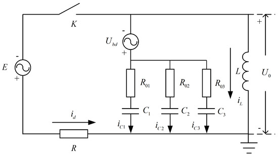
Figure 1 shows a transient equivalent circuit of a typical three-feeder resonant grounding system with a single-phase-to-ground fault [22].

Figure 1. Transient equivalent circuit of single-phase-to-ground fault.

Among them, $C_{1\sim 3}$ represents the capacitance to ground different feeders in the resonant grounding system. It is assumed that $C_1$ is the fault feeder. $R_{01\sim 03}$ represents the equivalent resistance of each feeder. $i_{C1\sim C3}$ represents the capacitive current of each feeder. $i_d$ represents the fault current flowing through the fault point. L represents the equivalent inductance of the arc suppression coil. $E=U_{m}sin({\omega }_{0}t+\phi )$ represents the source electromotive force of the fault phase when a single-phase-to-ground fault occurs in the system. $U_m$ represents the maximum phase voltage of the system. ${\omega }_0$ represents the system angular frequency. $\varphi$ represents the instantaneous phase at the fault occurrence time. $U_{bd}$ represents the three-phase unbalanced voltage of the system. R represents the transient resistance of a single-phase-to-ground fault. $U_0$ represents the neutral point voltage of the system. K represents the equivalent switch of the ground fault. If K is closed, it indicates that a single-phase-to-ground fault has occurred in the system. When switch K is open, that is, the system is running normally, only the three-phase unbalanced power supply $U_{bd}$ exists in the circuit. Correspondingly, the zero-sequence current phase of each feeder $i_{C1\sim C3}$ is only affected by the line impedance of each feeder. In actual lines, the impedances of each line are relatively small and can be approximately considered as $i_{C1\sim C3}$ in phase.

When switch K is closed, the fault phase power supply is connected, and the system transitions from steady state to the fault transient transition process. According to Figure 1, a linear constant coefficient second-order homogeneous differential equation is established as in (1). For convenience of calculation, the line resistance $R_{01\sim 03}$ is ignored. The derivation that follows is summarized from [22].

$$L{C}_0\frac{\mathrm{d}{i}_L^2}{\mathrm{d}{t}^2}+\frac{L}{R}\frac{\mathrm{d}{i}_L}{\mathrm{d}t}+i_L=\frac{1}{R}E+C_0\frac{\mathrm{d}{u}_{bd}}{\mathrm{d}t}$$

(1)

where $i_L$ represents the current flowing through the arc suppression coil, $C_0=C_1+C_2+C_3$ represents the sum of the capacitance to ground of all feeders, R represents the ground transition resistance, $u_{bd}$ represents the unbalanced voltage of the system, and t represents time. The characteristic roots are obtained by solving it as (2).

$$p_{1.2}=-\frac{1}{2R{C}_0}\pm \sqrt{{\left(\frac{1}{2R{C}_0}\right)}^2-\frac{1}{L{C}_0}}$$

(2)

Then the current flowing through the arc suppression coil can be expressed in the form of the general solution.

$${\dot{U}}_{bd}=-\frac{C_{\mathrm{A}}+{\alpha }^2·C_{\mathrm{B}}+\alpha ·C_{\mathrm{C}}}{C_0}·\dot{E}$$

(3)

where ${\dot{U}}_{bd}$ represents the vector expression form of the unbalanced voltage of the system, $C_{A\tilde{C}}$ represents the three-phase capacitance to ground, $\dot{E}$ represents the vector form of the fault phase electromotive force, and $\alpha =e^{-j{120}^{\circ }}$ represents the forward operator for 120°.

When the damping ratio ${\left(\frac{1}{2R{C}_0}\right)}^2-\frac{1}{L{C}_0}<0$ is greater than 1, the system operates in an overdamped state. When the damping ratio $R>\frac{1}{2}\sqrt{\frac{L}{C}}$ equals 1, the characteristic roots become a pair of conjugate complex numbers. Solving the differential equation yields the current flowing through the arc suppression coil.

$$i_L={\mathrm{e}}^{-\delta t}\left[A_{1}cos\left({\omega }_{f}t\right)+A_{2}sin\left({\omega }_{f}t\right)\right]+Bsin\left({\omega }_{0}t+\varphi \right)+Ccos({\omega }_{0}t+\theta )$$

(4)

where the damping coefficient is $\delta =\frac{1}{2R{C}_0}$, $A_1$ and $A_2$ are the general solution coefficients of the differential equation, B and C are the particular solution coefficients, the resonant frequency is ${\omega }_f=\sqrt{\frac{1}{L{C}_0}-{\left(\frac{1}{2R{C}_0}\right)}^2}$, and $\theta$ is the initial phase angle. The neutral point voltage can be expressed as:

$$\begin{array}{c}\hfill u_0=L\frac{\mathrm{d}{i}_L}{\mathrm{d}t}=-\left(\delta A_2+A_1{\omega }_f\right){\mathrm{e}}^{-\delta t}sin\left({\omega }_{f}t\right)+\left(A_2{\omega }_f-\delta A_1\right){\mathrm{e}}^{-\delta t}cos\left({\omega }_{f}t\right)+Bsin\left({\omega }_{0}t+\varphi \right)+Ccos({\omega }_{0}t+\theta )\end{array}$$

(5)

It can be seen from (5) that the transition process consists of two damped oscillating non-power frequency superimposed waves and two power frequency superimposed waves. The non-power oscillating frequency is close to the power frequency, which will form an obvious beat frequency characteristic. The amplitude is related to the resistance value of the transition resistance.

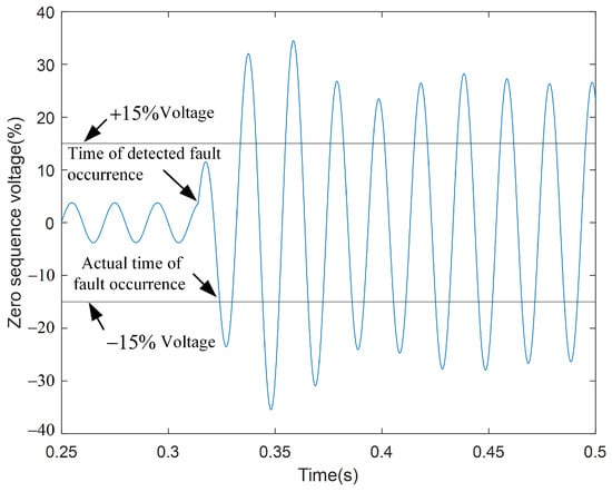
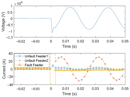
To illustrate with an example, when the three-phase unbalanced voltages of the system are $U_{bd}=123\mathrm{V}$, $C_0=24.7\mathsf{\mu }\mathrm{F}$, $L=0.5948\mathrm{H}$, and $R=1000\mathsf{\Omega }$, ${\left(\frac{1}{2R{C}_0}\right)}^2-\frac{1}{L{C}_0}=-67,657<0$. Use ATP/EMTP to establish a model as shown in Figure 1 for simulation, the zero-sequence voltage waveform is shown in Figure 2.

Figure 2. Fault detection delay due to Peterson coil.

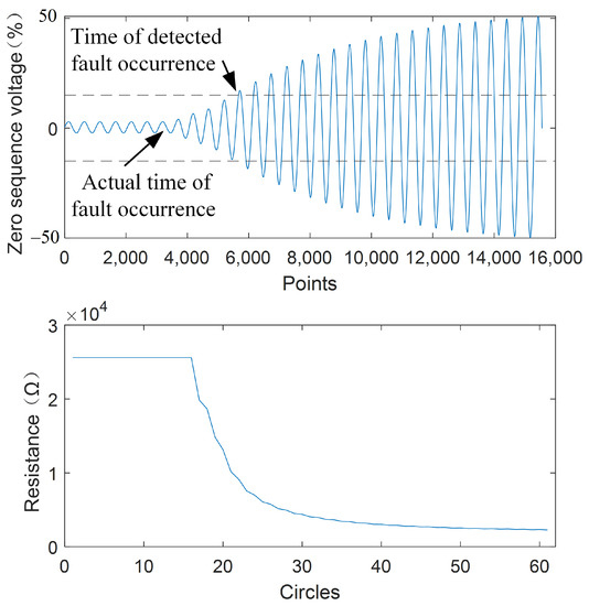
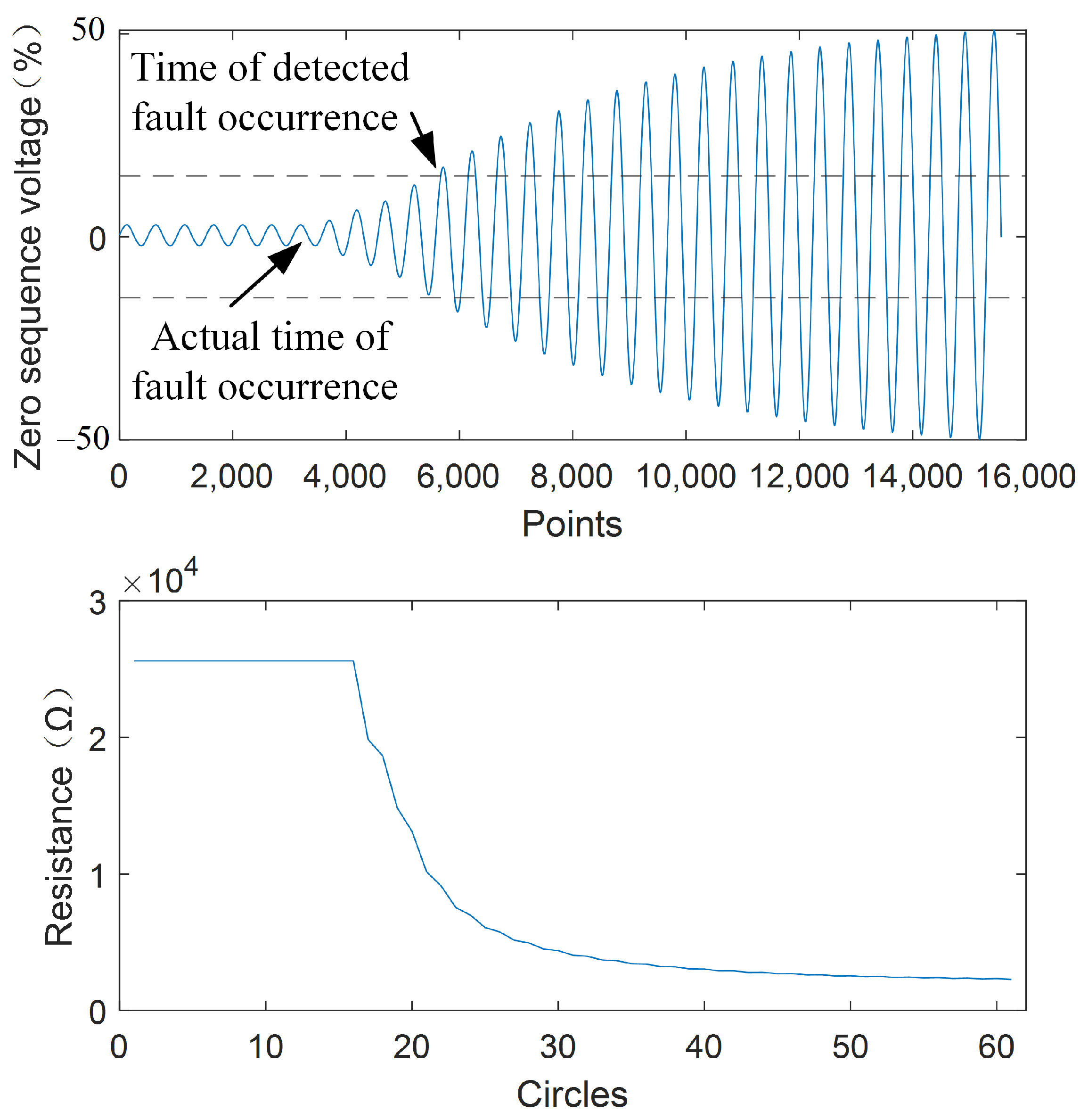
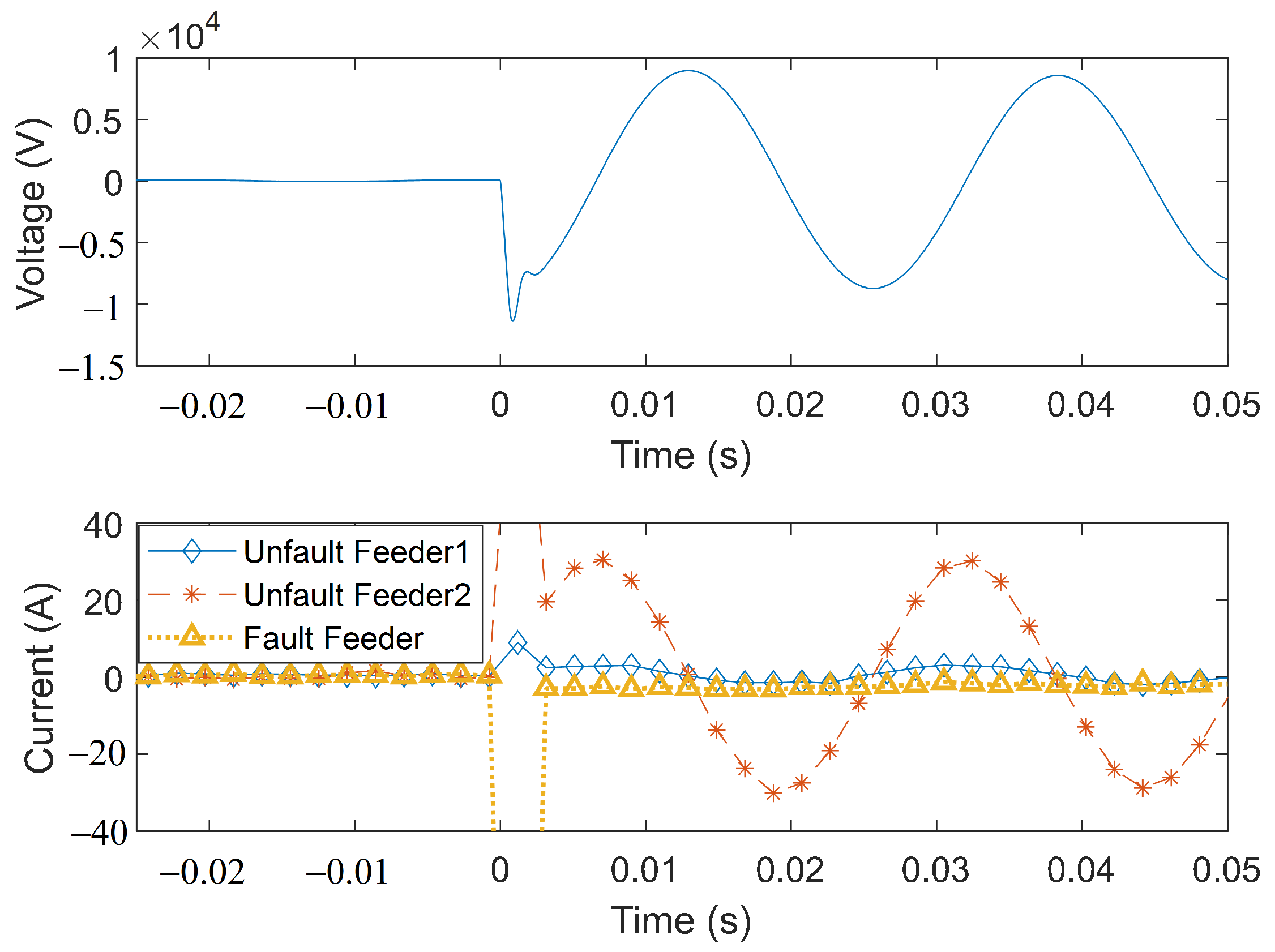
In reality, the transient resistance of a single-phase-to-ground fault does not jump from an insulated state to a fixed resistance but gradually transitions from an extremely large resistance to a steady-state resistance value. The transition process and the corresponding zero-sequence voltage waveform are shown in Figure 3.

Figure 3. Fault detection delay due to transition impedance.

It can be seen from the figure that under the dual effect of the transition resistance and the arc suppression coil, the start-up time detected by the zero-voltage threshold detection method is likely to lag behind the actual fault occurrence time. This makes it difficult for the fault line selection algorithm to extract the first half-wave data after the fault. For an ungrounded neutral point system, since the damping factor $\delta$ is large, the zero-sequence voltage rises very quickly. This lagging characteristic of zero-sequence voltage rise only exists in the neutral point grounded system via an arc suppression coil.

3. Identification Algorithm of Single-Phase-to-Ground Fault Occurrence Time

3.1. Zero-Sequence Current Signal Preprocessing Method Based on Empirical Mode Decomposition

Because high-impedance ground fault currents are small, they are easily affected by noise. There are two main sources of noise. The first is system background noise, mostly in the form of white noise. The second comes from CT measurement noise. When the current is below the minimum precision working current of the CT, the measured current will add a measurement error. The third is the possible existence of a DC component in the actual zero-sequence current, especially for short circuits with a small fault current, which has a greater impact.

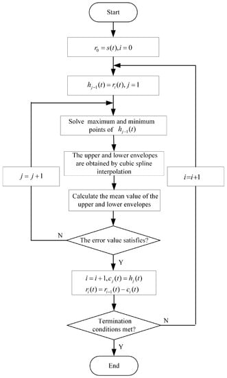
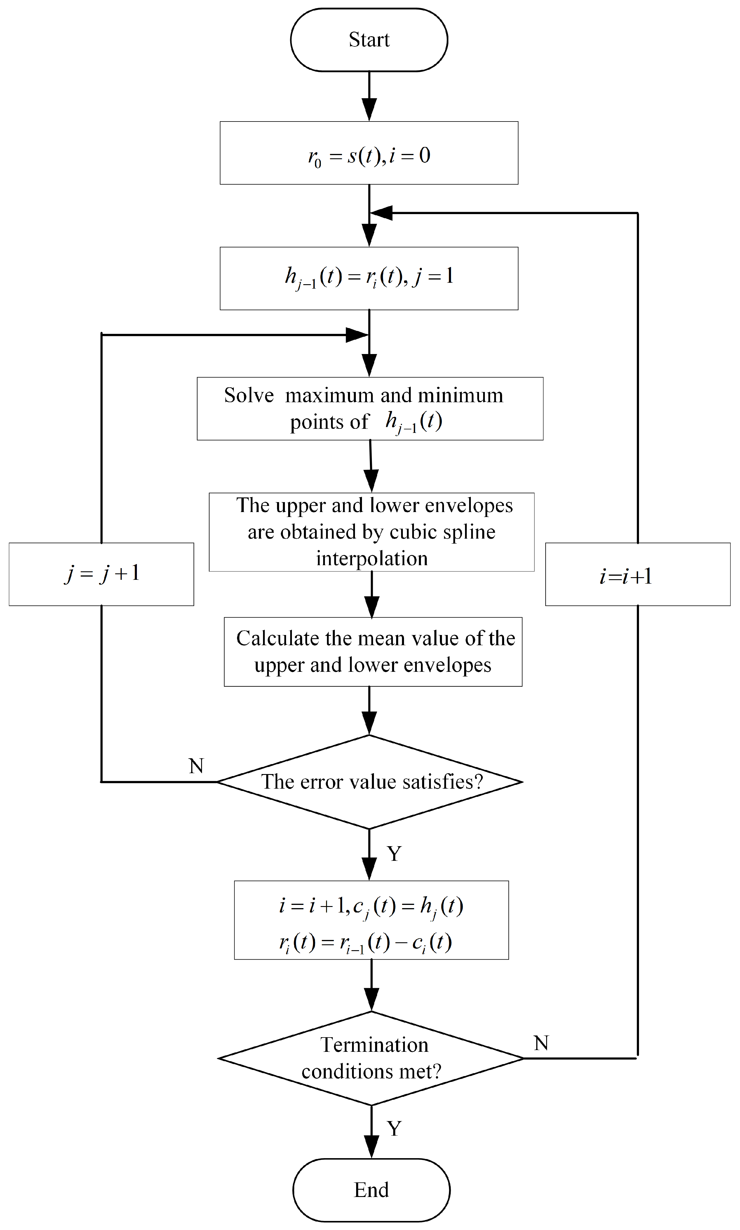
The EMD method is a frequency adaptive time series signal decomposition method. Its basic idea is to decompose an irregular frequency signal into the superposition of multiple quasi-frequency signals. Due to its adaptability in decomposing frequencies, this method is suitable for processing non-stationary zero-sequence current data generated by high-impedance ground faults. The implementation flowchart of the EMD algorithm is shown in Figure 4.

Figure 4. EMD algorithm flow chart.

The decomposition result of the EMD algorithm is several narrowband components (IMFs) with different frequencies, which can be expressed as several IMFs and a residual signal as (6) in [23].

$$x\left(t\right)=\sum _{i=1}^{n}im{f}_i\left(t\right)+r_n\left(n\right)$$

(6)

where ${\displaystyle \sum _{i=1}^n}im{f}_i\left(t\right)$ represents the sum of n IMF signals, and $r_n\left(n\right)$ represents the residual signal.

The EMD algorithm is a reversible decomposition, i.e., the original signal can be reconstructed by reassembling $im{f}_i\left(t\right)$, where $im{f}_1\left(t\right)\sim im{f}_n\left(t\right)$ corresponds to the decomposed signals from high to low frequency.

Combining Figure 1 and (5), the characteristic frequency of the feeder capacitive current is also composed of the damped oscillating non-power frequency signal ${\omega }_f=\sqrt{\frac{1}{L{C}_0}-{\left(\frac{1}{2R{C}_0}\right)}^2}$ and the power frequency signal ${\omega }_0$. ${\omega }_f$ is usually less than 250 Hz. Considering the frequency leakage problem that may exist in the EMD algorithm, to remove high-frequency noise and DC components that may interfere with the dimensionality reduction operation, the fast Fourier transform (7) is used to obtain the characteristic spectrum of $im{f}_i\left(t\right)$, and only the main spectrum within 25–200 Hz, $im{f}_i\left(t\right)$, is retained. By combining specific low-frequency IMF components, a low-pass filtering effect is achieved. It is worth noting that this characteristic frequency band is empirical, and for some special cases, it may be necessary to expand or narrow the range of the characteristic frequency band.

$$X_k=\sum _{n=0}^{N-1}im{f}_n{e}^{-i2\pi k\frac{n}{N}}k=0,\dots ,N-1$$

(7)

3.2. First Dimension Reduction Based on Principal Component Analysis

Compared with zero-sequence voltage, zero-sequence current has better transient characteristics after fault clearance and can more significantly distinguish between permanent and transient ground faults. However, a typical distribution network will have multiple feeders, which are not easy to analyze. It is necessary to extract the main component that can characterize this feature from the zero-sequence currents of all feeders.

This main component can be defined as a one-dimensional time series data feature that represents the variance contribution of the largest feature in all zero-sequence current data of the feeders [24]. Assuming there are m feeders and n zero-sequence current sampling points, the high-dimensional dataset $X_{n\times m}$ has m n-dimensional samples. The column data are the category, i.e., the feeder number, and the row data are the sample, i.e., the zero-sequence current sampling data.

Centering all sample data $x^{\left(i\right)}=\left(x^{\left(1\right)},x^{\left(2\right)},\dots ,x^{\left(m\right)}\right)$ of X, denoted as ${\displaystyle \sum _{i=1}^m}{x}^{\left(i\right)}=0$. We reduce the data dimension from n to 1, that is, the sample data $x^{\left(i\right)}$ are projected as $z^{\left(i\right)}=w^T{x}^{\left(i\right)}$ in a one-dimensional coordinate system, where $w^T$ is the projection operator representing the coordinates of the projection hyperplane. If $x^{\left(i\right)}$ is used to restore the original data, the recovered data ${\overline{x}}^{\left(i\right)}=z^{\left(i\right)}·w=W{z}^{\left(i\right)}$ can be obtained. The derivation that follows is summarized from [24].

Considering the whole sample set, we hope that all the sample data are close enough to the projection hyperplane, i.e., take the minimum value of (8).

$$\sum _{i=1}^m{∥{\overline{x}}^{\left(i\right)}-x^{\left(i\right)}∥}_2^2$$

(8)

Finishing available:

$$\begin{array}{cc}\hfill \sum _{i=1}^m{∥{\overline{x}}^{\left(i\right)}-x^{\left(i\right)}∥}_2^2& =-\sum _{i=1}^m{z}^{{\left(i\right)}^T}{z}^{\left(i\right)}+\sum _{i=1}^m{x}^{{\left(i\right)}^T}{x}^{\left(i\right)}\hfill \\ \hfill & =-\mathit{tr}\left(W^{T}X{X}^{T}W\right)+\sum _{i=1}^m{x}^{{\left(i\right)}^T}{x}^{\left(i\right)}\hfill \end{array}$$

(9)

In the formula, $tr$ represents the trace of a matrix, that is, the sum of the eigenvalues of the matrix. T denotes the matrix transpose. Minimizing the above formula is equivalent as.

$$\underset{W}{\underbrace{argmin}}-\mathit{tr}\left(W^{T}X{X}^{T}W\right)s.t.W^{T}W=I$$

(10)

In the formula, arg denotes the argument. $argmin$ represents the value of the coefficient matrix W that minimizes (8). I denotes the identity matrix. Using the Lagrangian function, we can obtain.

$$J\left(W\right)=-\mathit{tr}\left(W^{T}X{X}^{T}W+\lambda \left(W^{T}W-I\right)\right)$$

(11)

where $\lambda$ is the eigenvalue of the matrix X, and the derivative with respect to W gives

$$X{X}^{T}W=\lambda W$$

(12)

For the original dataset, we only need to use $z^{\left(i\right)}=W^T{x}^{\left(i\right)}$ to reduce the multi-dimensional zero-sequence current data to one-dimensional time series feature data.

3.3. Second Dimension Reduction Based on Hilbert Transform Mapping

The one-dimensional time series feature data are uniformly distributed in the time domain, making density-based feature clustering difficult. Therefore, a mapping transformation is needed.

For the one-dimensional time series feature dataset $z^{\left(i\right)}$ obtained by dimensionality reduction, it can be expressed as the time-based signal $z\left(t\right)$ as in [25].

$$z\left(t\right)={\int }_0^{\infty }A\left(\omega \right)cos(\omega t+\phi \left(\omega \right))\mathrm{d}\omega$$

(13)

where $\omega$ is the frequency of the signal, $\phi \left(\omega \right)$ is the initial phase angle of the frequency, and $A\left(\omega \right)$ is the amplitude of the frequency.

$$y\left(t\right)={\int }_0^{\infty }A\left(\omega \right)sin(\omega t+\phi \left(\omega \right))\mathrm{d}\omega$$

(14)

The feature dataset $z^{\left(i\right)}$, the Hilbert transform dataset $y^{\left(i\right)}$, and time $t^{\left(i\right)}$ constitute a three-dimensional dataset $q^{\left(i\right)}=\left(t^{\left(i\right)},y^{\left(i\right)},z^{\left(i\right)}\right)$. Projecting this dataset onto the YZ plane, a two-dimensional feature dataset is obtained by a second dimensionality reduction.

$$f^{\left(i\right)}=\left(z^{\left(i\right)},j·y^{\left(i\right)}\right)$$

(15)

where j is an imaginary unit.

3.4. Density-Based Clustering Fault Occurrence Time Identification Method

The two-dimensional feature dataset f can reflect the feature differences before and after the fault, but under different distribution systems or grounding fault conditions, the features are not exactly the same. Therefore, an adaptive fault boundary method is needed.

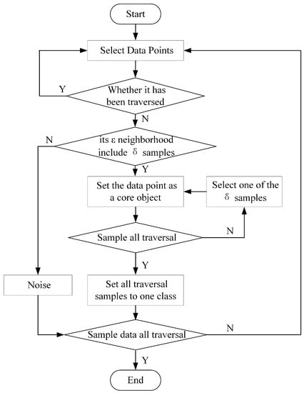
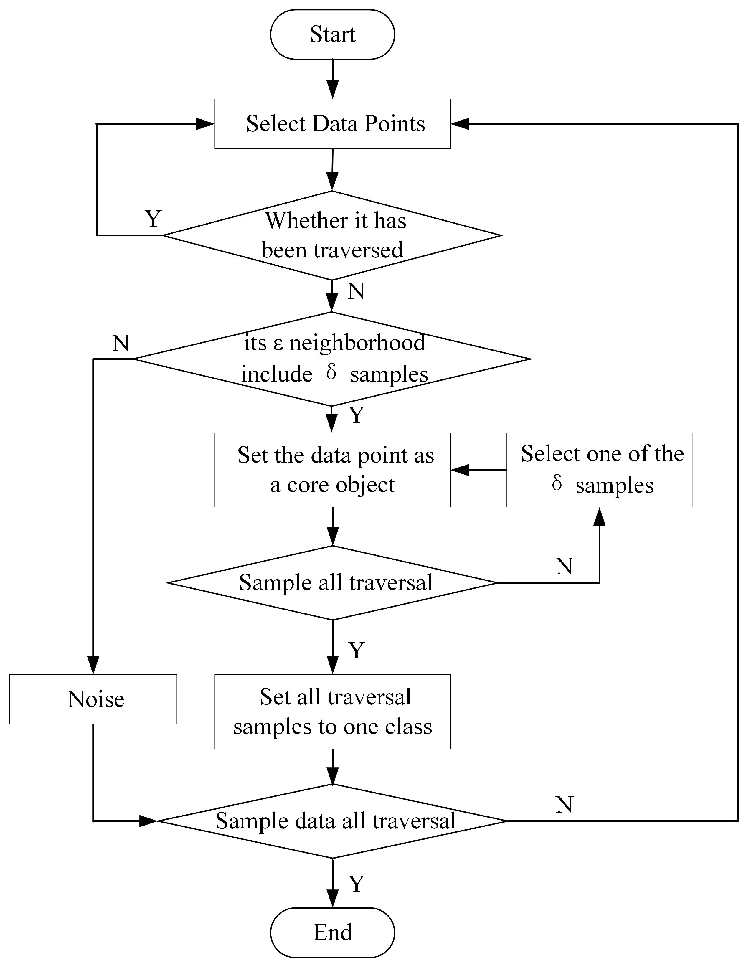
Since the data features obtained by the secondary dimensionality reduction projection have high density with non-fault data clustering together while the data gradually moves away from the non-fault data after the fault, this paper adopts a density-based clustering method to distinguish fault/non-fault data and obtain the fault time. The algorithm implementation flowchart is shown in Figure 5.

Figure 5. Density clustering algorithm flow chart.

Using the density clustering method, the reduced feature data are divided into two categories, one is non-fault data, and the other is fault data. The adjacent points between the two types of data are the detected fault times. Since the transient characteristics used for line selection mainly exist within the first half-wave (10 ms) after the fault occurs, the detected fault occurrence time within ±10 ms of the actual fault occurrence time can be considered reliable.

4. Verification of Accuracy of Single-Phase-to-Ground Fault Time Identification

4.1. Test Platform

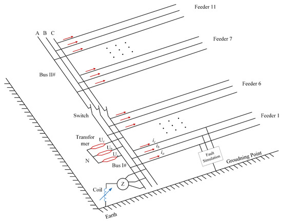
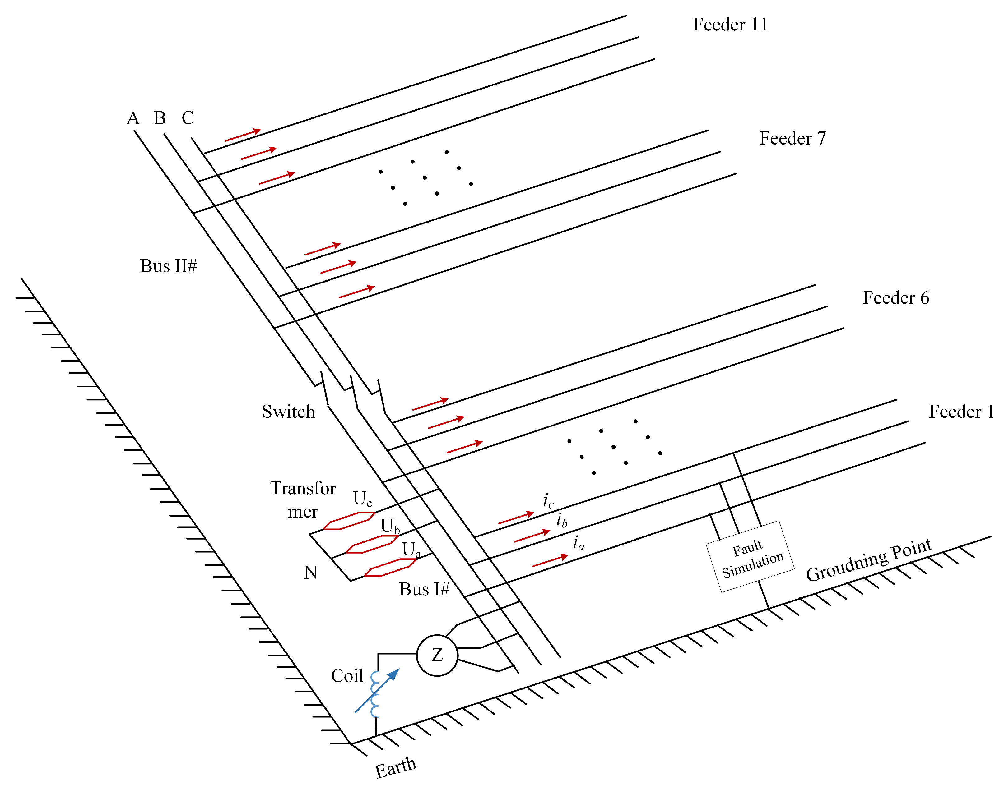
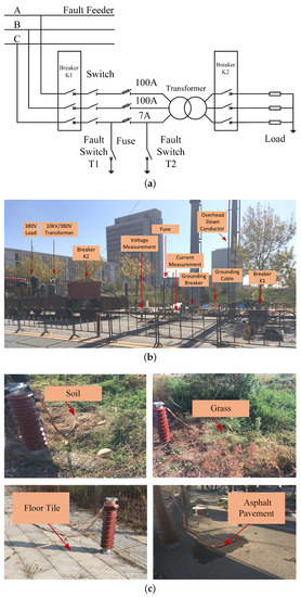
To fully verify the reliability of the detection method proposed in this paper, experimental validation was carried out based on a 66 kV substation shown in Figure 6. The substation is powered by a 50 MVA transformer. The substation has two main buses; Bus I has 6 feeders, and Bus II has 5 feeders, all of which are overhead lines. In the experiment, the two main buses were operated in parallel. The effective value of the system capacitive current was 68 A. On Bus I, a 700 kVA grounding transformer arc suppression coil set with a maximum compensation current of about 100 A was connected.

Figure 6. Experimental grid structure.

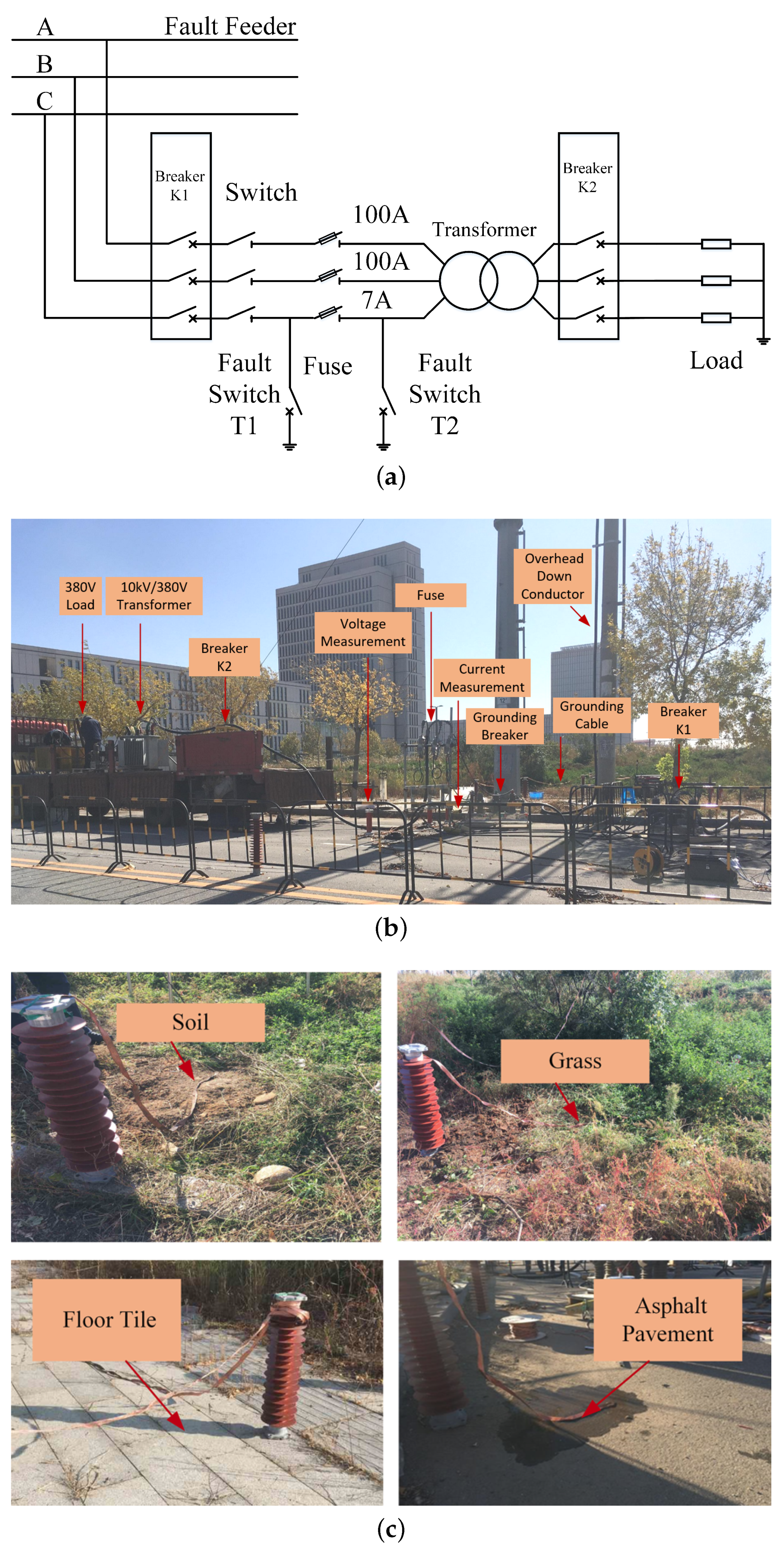
Feeder 1 on Bus I was selected as the fault simulation feeder. A 10 kV overhead line ground fault simulation platform was set up at its end. The fault simulation platform consists of circuit breaker $K1$, grounding switch $T1/T2$, circuit breaker K2, drop-out fuse, low-voltage resistor, etc. When simulating a line fault, 100 A fuses are used for phases A and B, and a 7 A fuse can be set for phase C. The system operates under load, causing the phase C fuse to blow. After blowing, the grounding switch $T1/T2$ simulates ground faults on the power supply side or load side after the line fault. Shorting the fuses simulates single-phase uninterrupted ground faults. The grounding switch in series with the fuse wire simulates transient ground faults. After the fault occurs, the fuse wire instantly fuses and clears the fault. The grounding media include soil, sand and stone, cement, branches, water pits, lawns, etc. The specific wiring methods and on-site layout of the platform are shown in Figure 7. On Bus I, feeders 1 and 6 were selected. On Bus II, feeders 7 and 11 were selected as measurement feeders to measure the three-phase currents $i_{abc}$ and zero-sequence current $i_0$ of four feeders, respectively.

Figure 7. Schematic diagram of ground fault simulation platform. (a) Grounding fault simulation platform wiring diagram. (b) Site layout of ground fault simulation platform. (c) Layout of grounding points for different media.

The 11 sets of experimental parameters are shown in Table 1. Negative residual current after compensation here refers to the arc suppression coil being in an overcompensated state, and the residual current is inductive and opposite to the system capacitive current direction.

Table 1. Experimental parameters.

Number	System Capacity Current (A)	Residual Current (A)	Grounding Mode	Medium
1	68	−7	Unbroken single-phase-to-ground	Soil
2	68	−7	Unbroken single-phase-to-ground	Sand
3	68	−7	Unbroken single-phase-to-ground	Cement
4	68	−7	Unbroken single-phase-to-ground	Tree Branch
5	68	−7	Unbroken single-phase-to-ground	Water
6	68	−7	Unbroken single-phase-to-ground	Tile
7	68	−26	Ground at the power supply side	Soil
8	68	−26	Ground at the power supply side	Grass
9	68	−26	Ground at the load side	Soil
10	68	−26	Ground at the load side	Grass
11	68	26	Single-phase-instantaneous-to-ground	Metal

4.2. Algorithm Sensitivity Verification

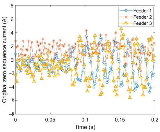
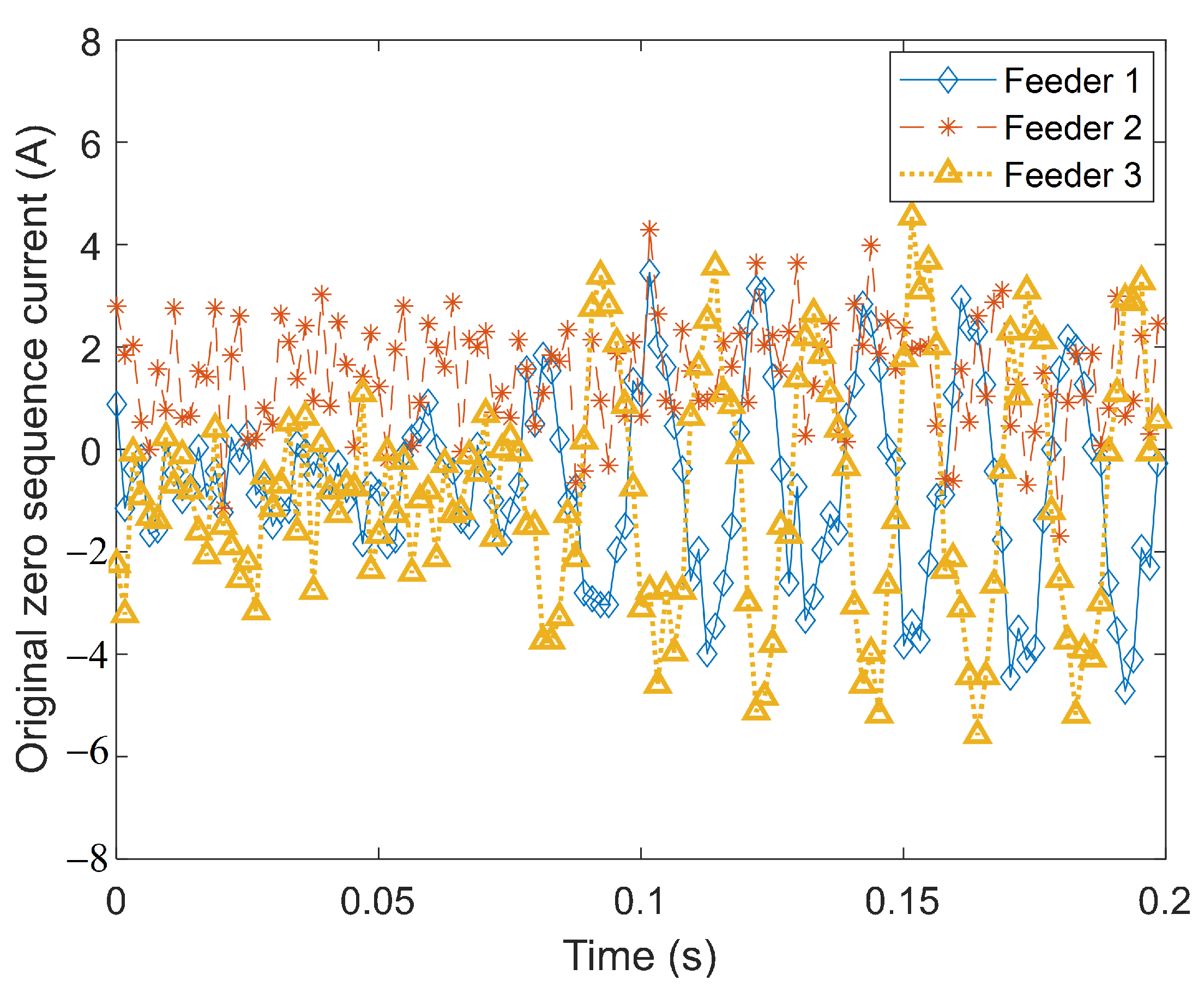
Taking experiment 2 as an example to verify the sensitivity of the detection algorithm proposed in this paper, the experiment has a large transitional resistor, resulting in a weak fault signal and severe noise interference. With 0.2 s as a complete sample period and a data sampling frequency $Fs=25.6$ kHz, the zero-sequence currents of each feeder are shown in Figure 8. For easy observation and comparison, only three are selected for display. The selected sample data are an 11-dimensional dataset with $n=2560$ and $m=11$.

Figure 8. Zero-sequence current of strong noise tree branches arcing grounding fault.

Preprocessing: The original data are decomposed using the EMD algorithm. The IMF components obtained are analyzed by spectral analysis. For I30 as an example, the signal is decomposed into 10 IMF components and 1 residual component. Only the IMF components with the main frequency spectrum within 25–200 Hz are retained, as shown in (16)

$$X=\sum _{i=6}^{10}IM{F}_i$$

(16)

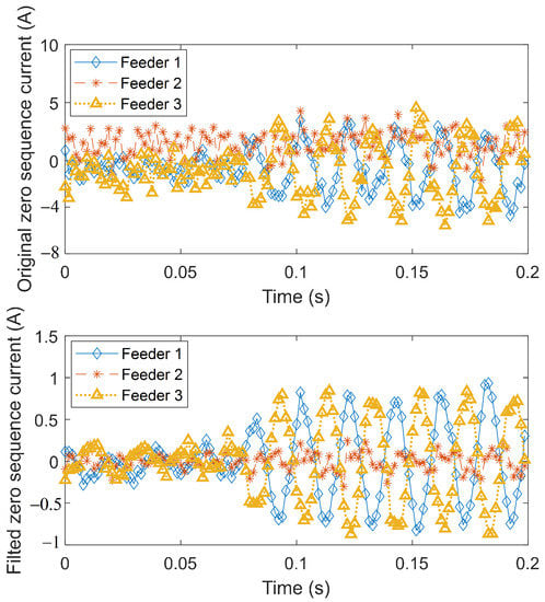
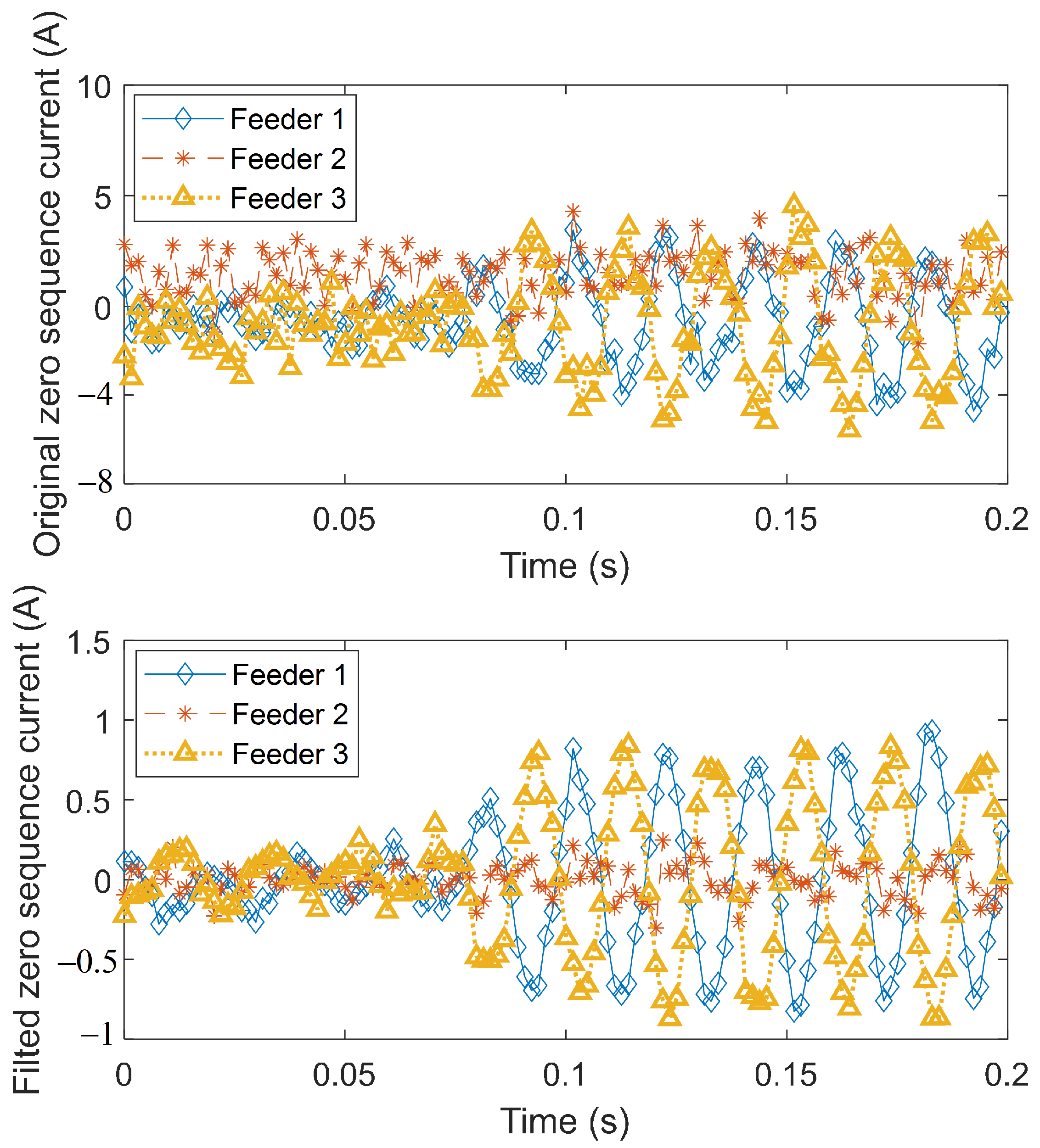
Figure 9 compares the original signal with the filtered signal, which removes most of the low-frequency noise and DC offset components.

Figure 9. Filter effect comparison chart.

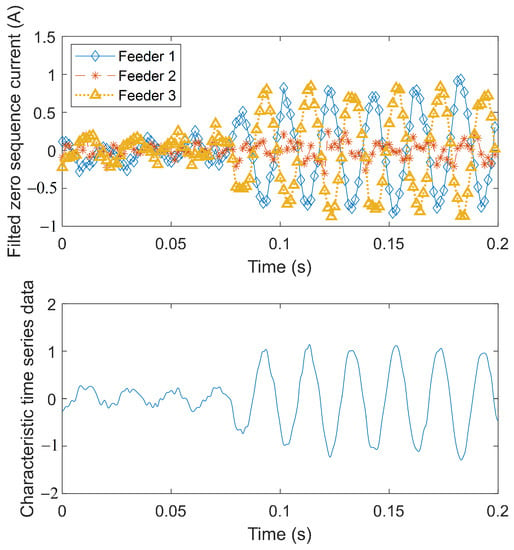
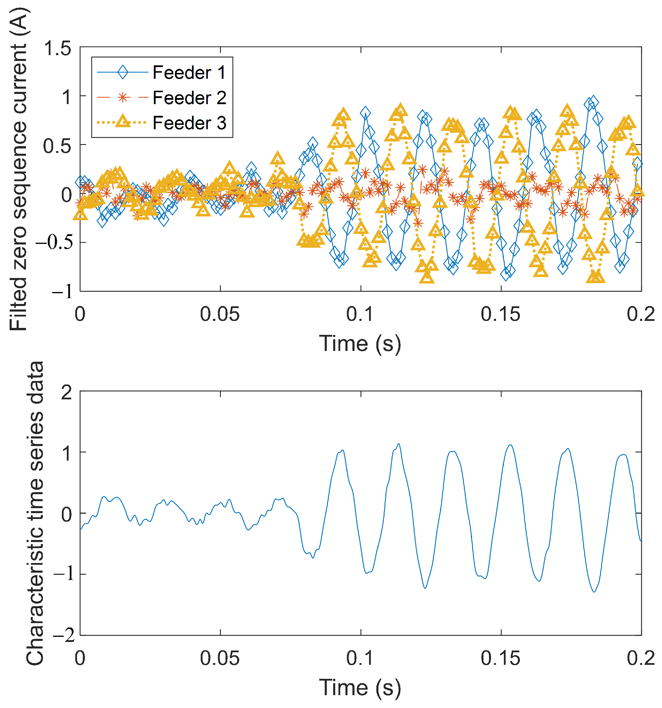
The first dimensionality reduction based on principal component analysis: The filtered dataset $X_{11\times 2560}$ is reduced to one-dimensional feature data $T_{1\times 2560}$ using the principal component analysis-based feature extraction algorithm proposed in this paper. Figure 10 shows the reduced-dimensional feature time series data.

Figure 10. First dimension reduction based on principal component analysis.

Although principal component analysis based on minimum variance theory can retain feature information well, some information loss is inevitable in the dimensionality reduction process. The variance explanation ratio is an important index to evaluate the contribution of principal components. Some studies have shown that when the sum of the variance explanation ratios of the selected principal components reaches $80\%$ or $90\%$, most of the reliable information in the original multidimensional data can be retained [26]. In this case, the principal component variance explanation ratio is $96.8\%$, indicating that most useful information is retained.

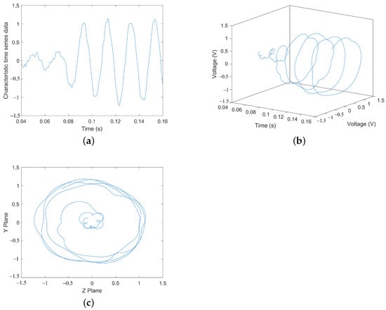
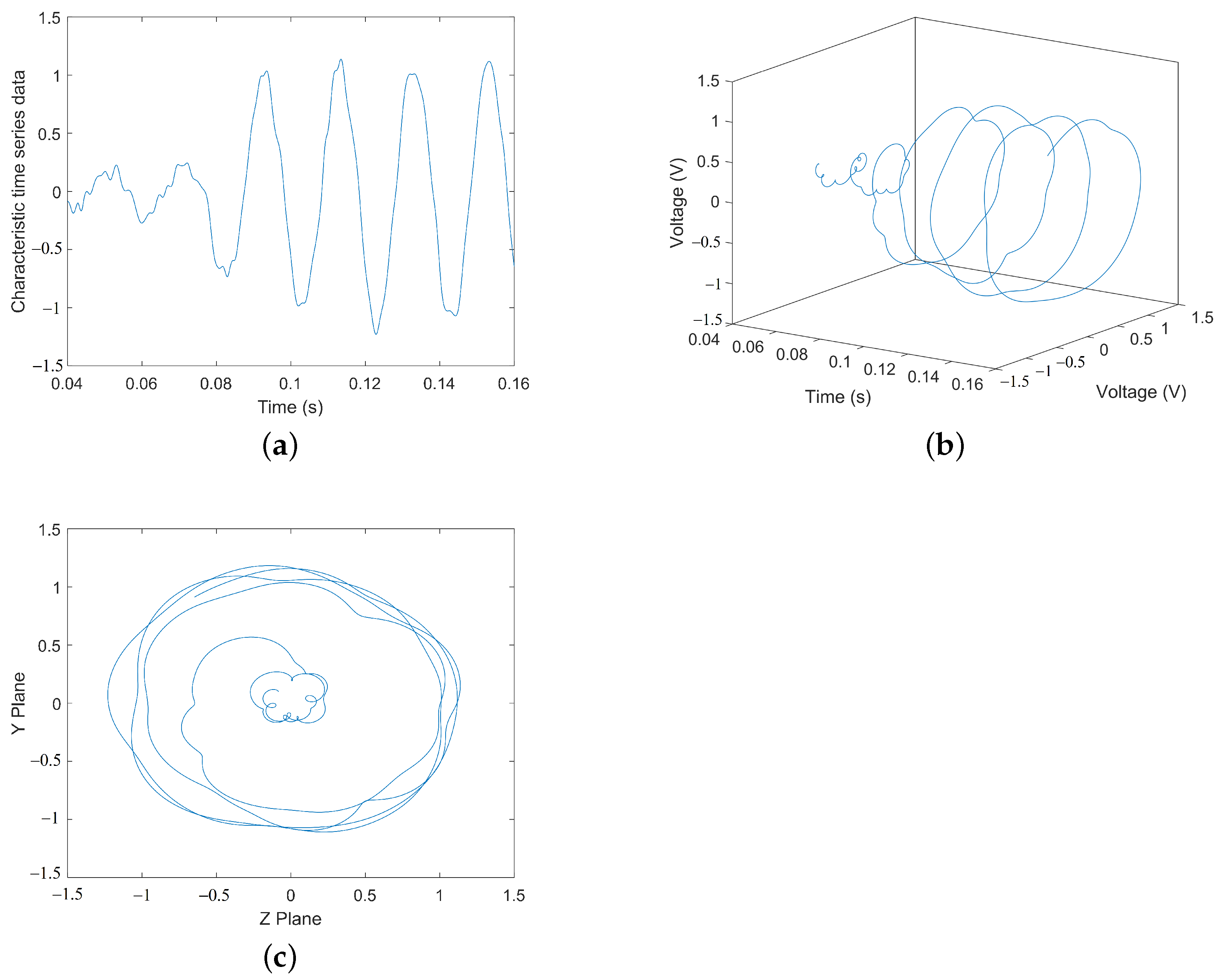
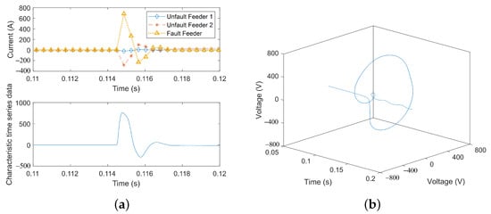
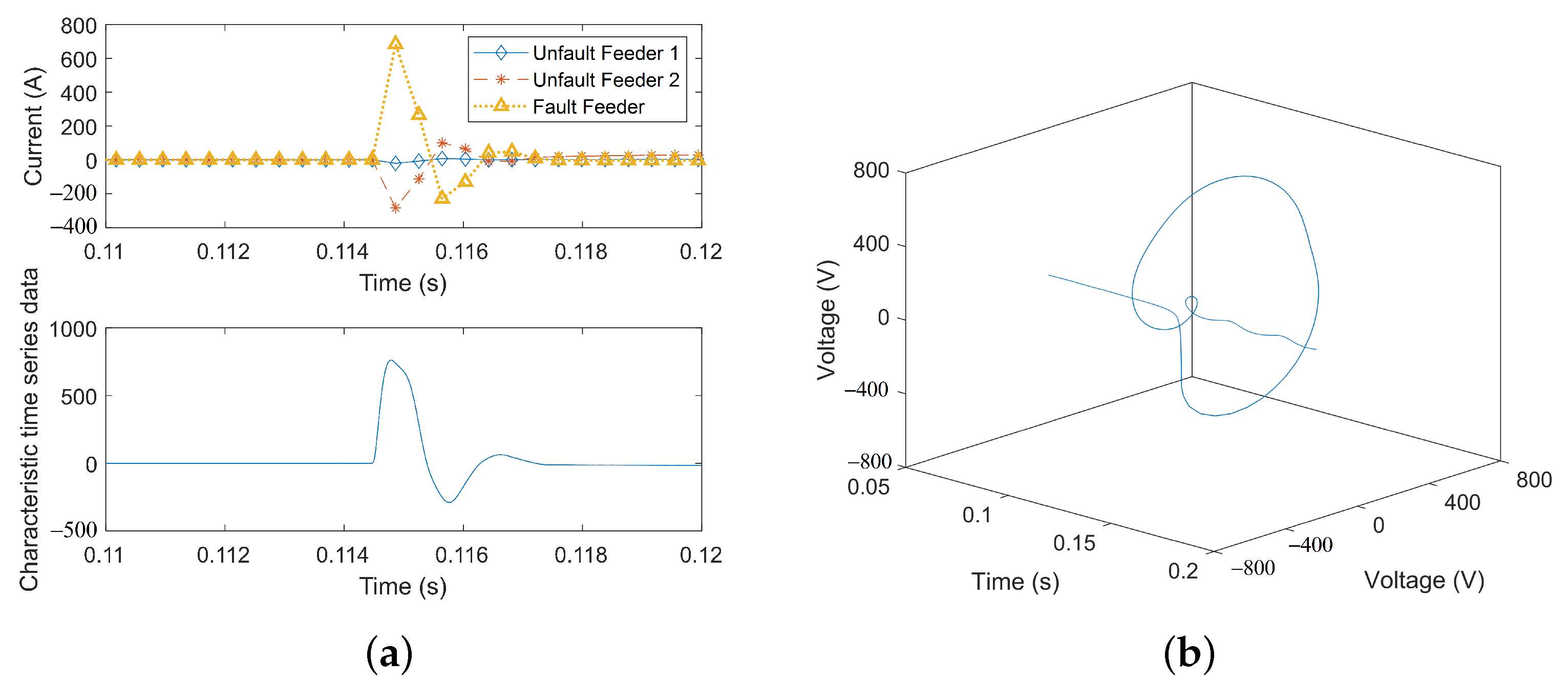
The second dimensionality reduction based on the Hilbert transform mapping: For the feature time series data after the first dimensionality reduction, the dimension is increased by the Hilbert transform and then projected onto the YZ plane for dimensionality reduction again. The schematic diagram of the dimensionality reduction process is shown in Figure 11.

Figure 11. Second dimension reduction based on Hilbert transform mapping. (a) Characteristic time series data. (b) Hilbert transform ascending dimension diagram. (c) YZ plane projection.

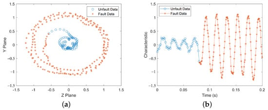
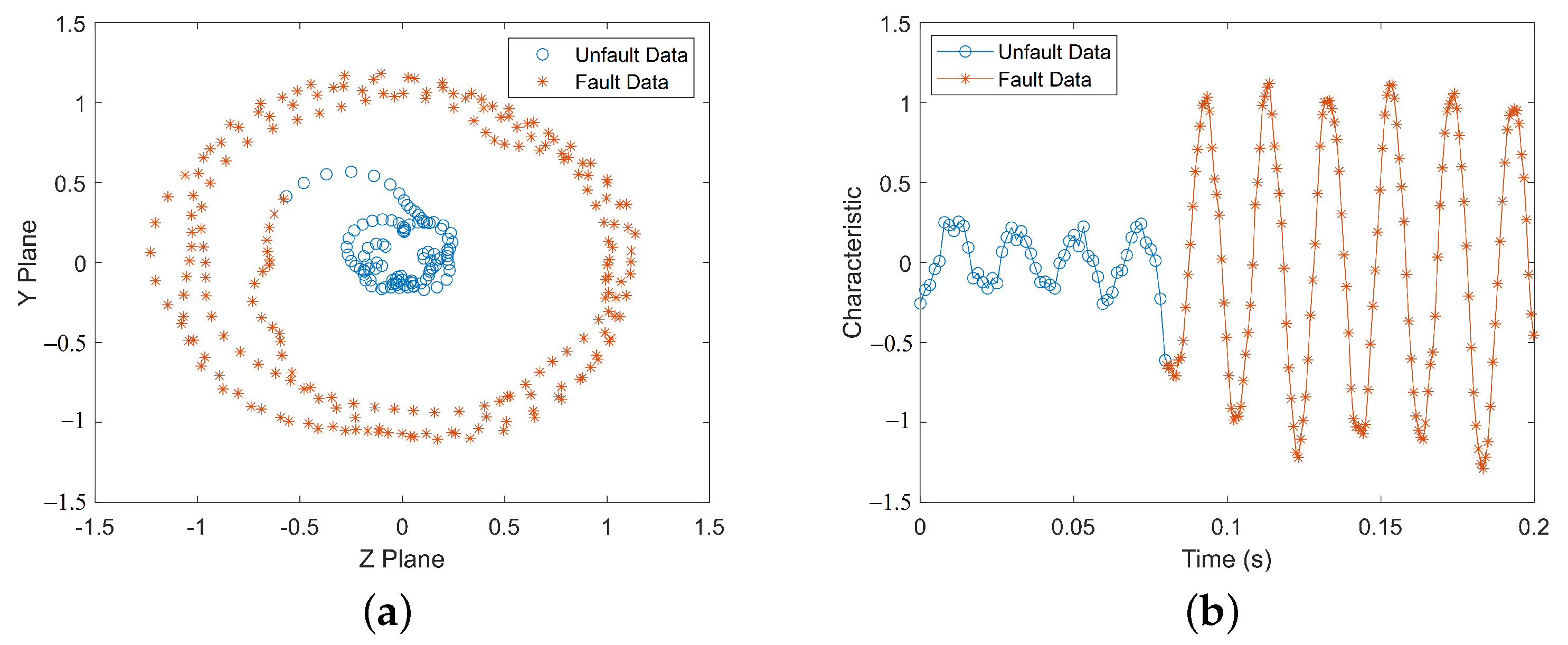
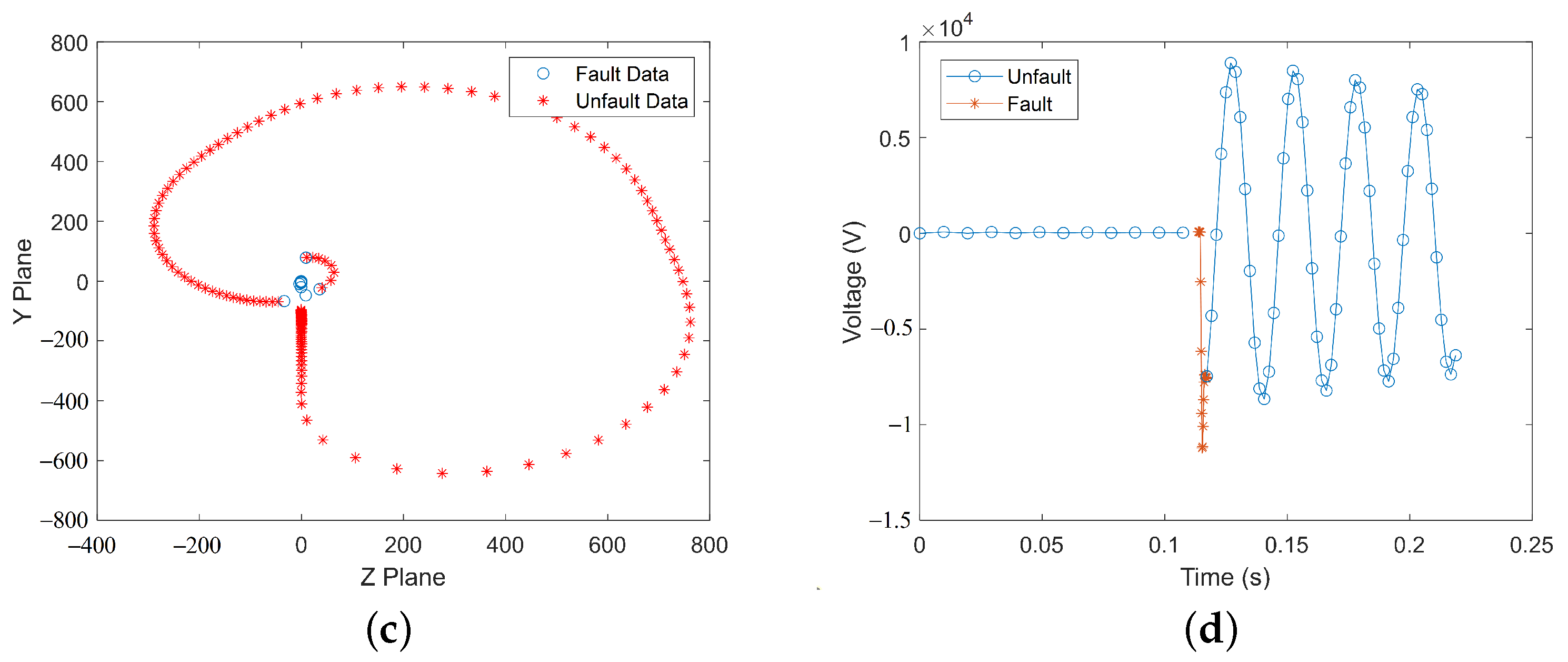
Fault occurrence time identification method based on density clustering: The twice reduced feature data are classified using the density clustering method proposed in this paper. Under the measurement data sampling rate of 25,600 Hz in this paper, the number of neighboring samples is set $\delta =100$. Experimental statistical results show that the neighborhood can take $\epsilon =0.35$ into account both local linear and global structural properties. The classification results are shown in Figure 12. The time point that divides the fault time and the non-fault time can be clearly displayed in the figure.

Figure 12. Fault occurrence time identification based on density clustering. (a) Density-based clustering effect map. (b) Schematic diagram of fault-time estimation.

4.3. Identification and Verification of Transient Faults

Figure 13 shows the attenuation curves of zero-sequence voltage and zero-sequence current of Group 11 test, instantaneous metallic single-phase-to-ground fault.

Figure 13. The attenuation curve of zero sequence voltage and zero sequence current of instantaneous metallic ground fault.

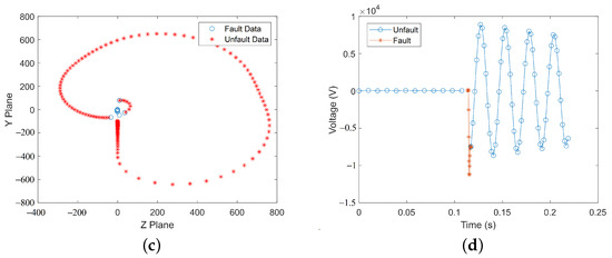
In a neutral-grounded distribution system through arc suppression coil grounding, the neutral point voltage will gradually decay after a transient ground fault occurs on a single phase. The decay rate is related to system parameters. In this experiment, a transient single-phase-to-ground fault occurred at 0 time. After $0.9$ s of fault occurrence, the neutral point voltage decayed to below $15\%$ of the phase voltage. According to the zero-sequence voltage percentage starting criterion, mis-starting may occur under such a fault condition. Figure 14 shows a schematic diagram of fault detection using the method proposed in this paper.

Figure 14. Effect diagram of fault detection based on two-step dimensionality reduction. (a) First dimension reduction based on principal component analysis. (b) Quadratic dimension reduction based on Hilbert transform. (c) Density-based clustering effect map. (d) Schematic diagram of fault-time estimation.

The method proposed in this paper is used to identify and classify transient ground faults. The feature data after two dimensionality reductions are clustered and analyzed on a two-dimensional plane. A clear separation point between fault data and non-fault data can be seen. After restoring to time-series data, this method can estimate the transient fault occurrence period relatively accurately.

4.4. Algorithm Stability Verification

The waveform data recorded in the first section of this chapter are used to test the performance of the algorithm under different operating conditions. Table 2 assumes that faults occur at 0 time and lists the fault occurrence times identified by the method proposed in this paper and the errors.

Table 2. Experimental results.

Experiments	Medium	Identify Fault Moment	Percentage of Post-Fault Neutral Voltage	Threshold Method Identification Time
single-phase-to-ground fault	Soil	0.75 ms	$14.1\%$	failed
single-phase-to-ground fault	Sand	7.3 ms	$4.4\%$	failed
single-phase-to-ground fault	Cement	0.05 ms	$4.9\%$	failed
single-phase-to-ground fault	Tree Branch	−0.85 ms	$6\%$	failed
single-phase-to-ground fault	Water	−5 ms	$9\%$	failed
single-phase-to-ground fault	Tile	−0.1 ms	$8.1\%$	failed
Ground fault at the power supply side	Soil	−2.7 ms	$35\%$	29 ms
Ground fault at the power supply side	Grass	−3.4 ms	$35\%$	8 ms
Ground fault at the load side	Soil	6.5 ms	$30\%$	6.3 s
Ground fault at the load side	Grass	4.5 ms	$21\%$	failed
Single-phase-instantaneous-to-ground	Metal	−0.7 ms	$15\%$ (0.9 s)	0.9 s

By comparing different ground fault media and different types of ground faults, the method proposed in this paper can effectively determine the fault occurrence state under any condition without missing tripping. It can effectively identify transient faults without misoperation. The identified fault occurrence time and the actual fault occurrence time are within 10 ms (half cycle) of each other. Compared to the commonly used industry method that detects faults based on a $15\%$ phase voltage threshold, this study chose more difficult fault scenarios in its experimental design. As a result, in most cases where a fault occurred, the zero-sequence voltage was below the $15\%$ phase voltage threshold, making the threshold-based detection method ineffective. However, in other fault scenarios, the fault-time estimation method proposed in this study demonstrated significant advantages.

5. Conclusions

For the problem of delayed start of the recloser due to a single-phase high-resistance grounding fault in a neutral grounding distribution system through an arc suppression coil, this paper introduces the idea of clustering method into fault detection and proposes a single-phase-to-ground fault-occurrence-time estimation algorithm based on two-stage dimensionality reduction. The main research conclusions are as follows:

(1)

There are features in the high-dimensional data composed of feeder zero-sequence currents that can be used to identify fault occurrence times. This algorithm performs feature extraction through two dimensionality reductions, amplifying the feature difference before and after the fault. The unsupervised density-based clustering algorithm can realize relatively accurate fault-time estimation.

(2)

This method can study dimensionality reduction for data of arbitrary dimensions. It has low dependence on the structure of the original dataset and is suitable for studying complex distribution networks. The dimensionality reduction process is repeatable with a clear mathematical theoretical meaning.

(3)

Experimental validation shows that this method can not only identify single-phase-to-ground faults but also has the ability to identify source-side grounding, load-side grounding, and transient grounding faults. The identification accuracy is within 7.3 ms, the experimental results presented in this study demonstrate that the proposed method exhibits better detection performance compared to the threshold detection method, which is able to effectively reduce the search range for fault characteristics in the selection process, and the method has a certain ability to cope with system noise.

In practical applications, after determining that a single-phase-to-ground fault has occurred in the system using the zero-sequence voltage threshold starting method, this method can be further applied to estimate the actual fault occurrence time more accurately and enhance the reliability of reclosers based on transient characteristics. It should be noted that accurate identification of the type of single-phase grounding fault is a prerequisite for the application of this method, and other similar fault characteristics, such as excitation current, should be avoided to prevent their impact on the results. The method proposed in this paper needs to set the number of adjacent samples and the neighborhood range, as well as the spectrum range retained by the EMD filtering algorithm. These parameters will affect the detection accuracy. Although empirical values obtained through experiments are given in the paper, how to adaptively adjust these parameters is an important issue for further study.

References

- Benner, C.L.; Russell, B.D. Practical high-impedance fault detection on distribution feeders. IEEE Trans. Ind. Appl. 1997, 33, 635–640. [Google Scholar] [CrossRef] [Scilit]
- Xu, Y.; Guo, M.; Chen, B.; Yang, G. Modeling and simulation analysis of arc in distribution network. Power Syst. Prot. Control 2015, 43, 57–62. [Google Scholar]
- Qiu, J.; Cui, X.; Tian, Y.; Wang, B.; Li, G. Analysis of the arc high impedance grounding faults voltage characteristics in non-effective grounding feeders. Power Syst. Prot. Control 2019, 47, 115–121. [Google Scholar]
- Bakar, A.H.A.; Ali, M.; Tan, C.; Mokhlis, H.; Arof, H.; Illias, H. High impedance fault location in 11 kV underground distribution systems using wavelet transforms. Int. J. Electr. Power Energy Syst. 2014, 55, 723–730. [Google Scholar] [CrossRef] [Scilit]
- Ghaderi, A.; Ginn III, H.L.; Mohammadpour, H.A. High impedance fault detection: A review. Electr. Power Syst. Res. 2017, 143, 376–388. [Google Scholar] [CrossRef] [Scilit]
- Wang, S.; Dehghanian, P. On the use of artificial intelligence for high impedance fault detection and electrical safety. IEEE Trans. Ind. Appl. 2020, 56, 7208–7216. [Google Scholar] [CrossRef] [Scilit]
- Tian, Y.; Xu, T.; Li, Y.; Deng, X.; Wang, Y. Fault line selection in a resonant earthed system based on reconstruction error and multi-scale cross-sample entropy. Power Syst. Prot. Control 2021, 49, 95–104. [Google Scholar]
- Liang, Y.L.; Li, K.J.; Ma, Z.; Lee, W.J. Typical fault cause recognition of single-phase-to-ground fault for overhead lines in nonsolidly earthed distribution networks. IEEE Trans. Ind. Appl. 2020, 56, 6298–6306. [Google Scholar] [CrossRef] [Scilit]
- Wu, W.; Zhang, X.; Zhang, J.; He, Y.; Bai, W. An improved Hausdorff distance method for locating single phase to ground fault in neutral non-effectively grounded system. IET Gener. Transm. Distrib. 2021, 15, 2747–2759. [Google Scholar] [CrossRef] [Scilit]
- Li, J.; Wang, G.; Zeng, D.; Li, H. High-impedance ground faulted line-section location method for a resonant grounding system based on the zero-sequence current’s declining periodic component. Int. J. Electr. Power Energy Syst. 2020, 119, 105910. [Google Scholar] [CrossRef] [Scilit]
- Chen, D.; Hu, B.; Li, Y.; Zhang, W.; Qi, Y.; Wang, R. Analysis of the Influence of Voltage Recovery Process on Line Selection Device When Single-phase Grounding Fault Is Removed. In Proceedings of the 2020 IEEE Sustainable Power and Energy Conference (iSPEC), Chengdu, China, 23–25 November 2020; pp. 1772–1777. [Google Scholar]
- Feng, G.; Guan, T.; Wang, L.; Xue, Y.; Yu, X.; Xu, B. Grounding fault line selection of non-solidly grounding system based on linearity of current and voltage derivative. Power Syst. Technol. 2021, 45, 302–311. [Google Scholar]
- Jiang, B.; Dong, X.; Shi, S. A method of single phase to ground fault feeder selection based on single phase current traveling wave for distribution lines. Proc. CSEE 2014, 34, 6216–6227. [Google Scholar]
- Jiang, B.; Dong, X.; Shi, S.; Wang, B. A Method of Adaptive Time Frequency Window Traveling Wave Based Fault Feeder Selection. Proc. CSEE 2015, 35, 6837–6897. [Google Scholar]
- Fang, Y.; Xue, Y.; Song, H.; Guan, T.; Yang, F.; Xu, B. Transient energy analysis and faulty feeder identification method of high impedance fault in the resonant grounding system. Proc. CSEE 2018, 38, 5636–5645. [Google Scholar]
- Wei, M.; Shi, F.; Zhang, H.; Jin, Z.; Terzija, V.; Zhou, J.; Bao, H. High impedance arc fault detection based on the harmonic randomness and waveform distortion in the distribution system. IEEE Trans. Power Deliv. 2019, 35, 837–850. [Google Scholar] [CrossRef] [Scilit]
- Ghaderi, A.; Mohammadpour, H.A.; Ginn, H.L.; Shin, Y.J. High-impedance fault detection in the distribution network using the time-frequency-based algorithm. IEEE Trans. Power Deliv. 2014, 30, 1260–1268. [Google Scholar] [CrossRef] [Scilit]
- Liu, Y.; Liu, X.; Fan, S.; Ma, X.; Deng, S. Single-phase-to-ground fault line selection method based on STOA-SVM. J. Phys. Conf. Ser. 2021, 2095, 012029. [Google Scholar] [CrossRef] [Scilit]
- Wei, H.; Wei, H.; Lyu, Z.; Bai, X.; Tian, J. Deep Belief Network Based Faulty Feeder Detection of Single-Phase Ground Fault. IEEE Access 2021, 9, 158961–158971. [Google Scholar] [CrossRef] [Scilit]
- Liang, Y.; Li, K.J.; Ma, Z.; Lee, W.J. Multilabel classification model for type recognition of single-phase-to-ground fault based on KNN-Bayesian method. IEEE Trans. Ind. Appl. 2021, 57, 1294–1302. [Google Scholar] [CrossRef] [Scilit]
- Fan, M.; Xia, J.; Meng, X.; Zhang, K. Single-phase grounding fault types identification based on multi-feature transformation and fusion. Sensors 2022, 22, 3521. [Google Scholar] [CrossRef] [Scilit]
- Xue, Y.; Li, J.; Xu, B. Transient equivalent circuit and transient analysis of single-phase earth fault in arc suppression coil grounded system. Proc. CSEE 2015, 35, 5703–5714. [Google Scholar]
- Boudraa, A.O.; Cexus, J.C. EMD-based signal filtering. IEEE Trans. Instrum. Meas. 2007, 56, 2196–2202. [Google Scholar] [CrossRef] [Scilit]
- Wang, N.; Wang, S.; Jia, Q. The method to reduce identification feature of different voltage sag disturbance source based on principal component analysis. In Proceedings of the 2014 IEEE Conference and Expo Transportation Electrification Asia-Pacific (ITEC Asia-Pacific), Beijing, China, 31 August–3 September 2014; pp. 1–6. [Google Scholar]
- Jie, Z.; Jian, L.; Hongtao, Z.; Yue, S. Sinusoidal representation of transient signal based on Hilbert transform. In Proceedings of the 2021 IEEE International Conference on Data Science and Computer Application (ICDSCA), Dalian, China, 29–31 October 2021; pp. 280–285. [Google Scholar]
- Jolliffe, I.T. Principal Component Analysis for Special Types of Data; Springer: Berlin/Heidelberg, Germany, 2002. [Google Scholar]
Disclaimer/Publisher’s Note: The statements, opinions and data contained in all publications are solely those of the individual author(s) and contributor(s) and not of MDPI and/or the editor(s). MDPI and/or the editor(s) disclaim responsibility for any injury to people or property resulting from any ideas, methods, instructions or products referred to in the content. |
© 2023 by the authors. Licensee MDPI, Basel, Switzerland. This article is an open access article distributed under the terms and conditions of the Creative Commons Attribution (CC BY) license (https://creativecommons.org/licenses/by/4.0/).