The Estimation Life Cycle of Lithium-Ion Battery Based on Deep Learning Network and Genetic Algorithm

Abstract

This study uses deep learning to model the discharge characteristic curve of the lithium-ion battery. The battery measurement instrument was used to charge and discharge the battery to establish the discharge characteristic curve. The parameter method tries to find the discharge characteristic curve and was improved by MLP (multilayer perceptron), RNN (recurrent neural network), LSTM (long short-term memory), and GRU (gated recurrent unit). The results obtained by these methods were graphs. We used genetic algorithm (GA) to obtain the parameters of the discharge characteristic curve equation.

1. Introduction

Energy demand is increasing, from power generation to today’s nuclear power generation. In recent years, environmental protection issues have gradually risen and environmental pollution caused by power generation has become a threshold that must not be crossed by technological development [1].

To achieve convenience, countless devices have been invented, which use electrical energy as the main source. People have invented, improved, and simplified these devices. Portable electronic products can integrate various high-tech features. Modern high-tech products can be seen everywhere such as notebook computers, mobile phones, navigation devices, smart-watches, tablet computers, etc. To realize these elements, the battery is an indispensable component [2].

Nowadays, batteries are used in almost every device, which leads to a significant impact on the environment. Therefore, it would be ideal to optimize these reusable batteries. The time and endurance of the device are dependent on reusable batteries. In addition to emphasizing the large capacity and long life of the battery, the market is also committed to research on battery health management systems. An automatic power-off system for charging can prevent the battery from overcharging and preventing the problem of reduced battery life [3,4,5].

In recent years, different energy storage equipment has been developed but some challenges remain. These challenges include the reduction in the cost of energy storage equipment and its size, extended lifespan and improved performance, and the system for measuring the remaining battery power. Each discharge characteristic curve is different for different manufacturers. It is very important to establish a battery discharge characteristic module. To build a battery model, we need to understand the health of the battery, the discharge current, and the battery capacity. Then, the life of the battery can be predicted.

As it is difficult to build a battery model, the voltage is measured at different time points with different current levels. To reduce time and cost, deep learning was used to solve the problem. We used different deep learning algorithms to train our model and to find the most similar characteristic curve.

The discharge characteristic curve of the lithium-ion battery has been modeled by several methods [3,4,5] including the discharge test [6], ampere hour counting [4], open circuit voltage [4], linear modeling [7], physical properties of the electrolyte [4], internal resistance [4], impedance spectroscopy [8], Kalman filter [9], and artificial intelligence [10,11]. The methods of the discharge test, ampere hour counting, open circuit voltage, impedance spectroscopy, Kalman filter, and artificial intelligence are suitable for all battery modeling, which have the advantages of online and easy to accurate, but have the drawbacks of adjusting the battery state, needing regular re-calibration points, low dynamics, cost intensive, the problem of determining initial parameters, and needing the training data, respectively. The method of linear modeling, the physical properties of the electrolyte and the internal resistance are usually in the application of lead, Ni/Cd, and Zn/Br batteries, which are not suitable for lithium-ion batteries [4].

The goal of our study was to predict the different model battery life based on the optimization algorithm and deep learning method. We adopted the optimization algorithm to find different battery charge and discharge regression parameters and used recurrent a deep neural network to predict the real discharge battery lifetime. Another objective is our hope that these studies can help in the prediction of electric vehicle batteries.

This paper used different deep learning methods to study the discharge behavior of the battery to establish a discharge model and to understand the characteristics of the battery discharge. The measured discharge characteristic curve value was input into multilayer perceptron, recurrent neural network, long short-term memory, gated recurrent unit, and genetic algorithm, which are five different algorithms for training. The parameter values obtained were then compared with the characteristic values of the originally measured discharge curve.

The rest of this article is organized as follows. Section 1 describes our study motivation and Section 2 introduces the related works about battery life prediction. Section 3 contributes to our proposed method. The experimental section excludes our different battery model. Finally, we conclude our results in the last section.

2. Related Works

In recent years, the use of artificial intelligence has greatly increased in the application of modeling the discharge of lithium-ion batteries [4,5,11]. Artificial intelligence is realized among the methods of machine learning and deep learning. Deep learning is a training method of machine learning and is the main mode of operation of artificial intelligence today. In this era of automation, the application of deep learning can be seen everywhere [12].

Since the 1980s, the reduction in computer hardware costs and the advancement of storage equipment has helped machine learning to flourish. It has evolved from a single-layer network to the current multi-layer network [13].

Deep learning is used for image recognition in self-driving cars. For artificial intelligence, the real challenge lies in how to solve the problem intuitively for humans. The image recognition based on deep learning can be retrieved as efficient features by convolution operators because some features are difficult for humans to extract. Deep learning has evolved and has been improved and simplified. There are many algorithms and models for everyone to apply because different algorithms or models have different characteristics, training methods, performance, and efficiency.

2.1. MLP (Multilayer Perceptron)

Multi-layer perceptron is a supervised learning algorithm. The multi-layer architecture deals with nonlinear problems. MLP is roughly divided into three levels: input layer, hidden layer, and output layer. Each neuron is fully connected, and each connected neuron has weights that are used to calculate whether the input data has the information we need [14,15,16].

2.2. RNN (Recurrent Neural Network)

The recurrent neural network was invented by David Rumelhart in 1986 [17]. It is roughly divided into three levels: input layer, state layer, and output layer. The state layer can also be regarded as a hidden layer, but the difference from MLP is that the state layer of RNN will have one more output value of the previous layer as input. Therefore, RNN is a kind of neural network with short-term memory [11,16,18,19].

RNN is a kind of neural network that is good at dealing with sequence problems. It specializes in dealing with related topics such as weather observation, stock trading, video data, and other temporal data. RNN emphasizes a concept: if a specific message appears multiple times in a sequence, then the matter of sharing information will become extremely important.

RNN has a vanishing gradient problem. When the program is performed longer, the earlier data will become less important. This results in the incomplete calculation of the weights and the entire program cannot be carried out. It is impossible to remember what happened a long time ago. This problem was solved by Sepp Hochreiter and Jürgen Schmidhuber, who invented LSTM to improve the vanishing gradient problem.

2.3. LSTM (Long Short-Term Memory)

LSTM is a special RNN model proposed by Sepp Hochreiter and Jürgen Schmidhuber in 1997 to improve the vanishing gradient problem [20]. Compared to RNN, LSTM is complicated. This algorithm introduces three gates to control memory, namely input gate, forget gate, and output gate. It gives the machine an ability to select information [21,22,23,24]. Here, we must mention three types of activation functions commonly used in deep learning. The commonly used activation functions in deep learning are the sigmoid function, tanh function, and rectified linear unit (ReLU). Sigmoid function is monotonous, continuous, and easy to solve [25]. The disadvantage of this function is that it can cause the vanishing gradient problem in the saturated regions at both ends. The advantages of the tanh function are similar to the sigmoid function, but the slope of the tanh function is larger, and the convergence and training speed will be faster [26]. The training range is from −1.0 to 1.0, so a more approximate value can be found. The disadvantage is the same as that of the sigmoid function (i.e., a vanishing gradient problem). The activation function rectified linear unit (ReLU) has no vanishing gradient problem and no complicated exponential calculations [27] with a fast convergence rate. The disadvantage of ReLU is that when the input is less than zero, it will not be able to update the data for the next calculation.

2.4. GRU (Gated Recurrent Unit)

The gated recurrent unit is a type of recurrent neural network. It was invented by Junyoung Chung et al. in 2014 [28]. Like LSTM, it is designed to solve the vanishing gradient problem. The biggest difference is that this algorithm combines the forget gate and the input gate and replaces it with an update gate. Because of this, the GRU required calculation time and the required resources are greatly reduced [29,30,31,32].

The following table shows the three model (RNN, LSTM, and GRU) equations, separately. The below table shows the RNN, LSTM, and GRU equations.

Recurrent Neural Network Equation

The output of RNN: $h_t=\mathsf{\sigma }\left(U_h\times X_t+W_h\times h_{t-1}+b_h\right)$ σ( ) is activation function. $h_t$ is the hidden layer activations in time t. $X_t$ is the input vector. $U_h$ is the weight of input vector. $W_h$ is the weight of hidden layer activations. $b_h$ is the bias.

Long Short Term Memory Equation

Forgotten gate: $f_t=\mathsf{\sigma }\left(W_{xf}\times X_t+W_{hf}\times h_{t-1}+b_f\right)$ σ( ) is activation function. $f_t$ is the current forgotten gate. $X_t$ is the current input vector. $W_{xf}$ is the current weight of input vector. $W_{hf}$ is the weight of the hidden vector. $h_{t-1}$ is the weight of hidden vector in time t − 1. $b_f$ is the bias. Input gate: it = σ(Wxi × Xt + Whi × ht − 1 + bi) $s_{\mathrm{t}}=i_{\mathrm{t}}\ast \mathsf{\sigma }\left(W_{xs}\times X_t+W_{hs}\times h_{t-1}+b_s\right)+{\mathrm{f}}_{\mathrm{t}}\ast s_{\mathrm{t}-1}$ it is the external input gate. Output gate: Ot = σ(Wxo × Xt + Who × ht − 1 + bo) $h_t=O_t\times tanh\left(s_t\right)$ Ot is the output gate. $h_t$ is the output.

Gated Recurrent Unit Equation

Update gate: $Z_t=\mathsf{\sigma }\left(W_z\times X_t+W_z\times h_{t-1}+b_z\right)$ Zt is the update gate. Reset gate: $R_t=\mathsf{\sigma }\left(W_r\times X_t+W_r\times h_t-1+b_r\right)$ Rt is the reset gate.

3. Our Proposed Battery Model and Prediction Method

Through the description in the previous section, we found that the recurrent deep neural network had better prediction performance and the battery life was a sequential predicted problem. Therefore, our study must discover different battery parameters with a battery regression function, so we designed a battery charge or discharge activation process to discuss the battery characteristics. We also introduced our major optimization algorithm—genetic algorithm—to help us to find the parameters of the battery charge/discharge function.

3.1. Battery Characteristics

This paper used 18,650 commercial lithium-ion cylindrical batteries, which were common brands with good reliability and currently available on the market. We named them L brand, P brand, and S brand. The basic specifications and charging and discharging conditions are shown in Table 1. The charge cut-off voltage was 4.2 V and the discharge cut-off voltage was 3 V.

Table 1. Specifications for 18,650 commercial lithium-ion cylindrical batteries.

	L Brand	P Brand	S Brand
Average voltage	3.7 V	3.7 V	3.7 V
Charging cut-off voltage	4.2 V	4.2 V	4.2 V
Discharge cut-off voltage	3.0 V	3.0 V	3.0 V
Nominal capacity	2200 mAh	2200 mAh	2200 mAh
Maximum discharge rate	1.5 C	1.5 C	1.5 C
Cycle life	≥300	≥300	≥300
Charging working temperature	10 °C~45 °C	10 °C~45 °C	10 °C~45 °C
Discharge working temperature	−10 °C~60 °C	−10 °C~60 °C	±10 °C~60 °C

3.2. Lithium-Ion Battery Charge and Discharge

After understanding the charging and discharging conditions of the battery, one can use the battery tester to set multiple groups of different charging and discharging rates as an electronic load to test the battery characteristics of a single battery core. Automated battery testing equipment can be used to measure various parameters of the battery in operation (such as voltage, current, current flow, and battery surface temperature, etc...), analyze these data to understand battery characteristics, and build battery characteristics data based on this fuel gauge model [3].

3.3. Lithium-Ion Battery Activation

Since the selected lithium-ion battery was used for the first time, the lithium-ion battery had to be activated before the charge and discharge study as the measured charge and discharge characteristics can reflect the characteristics of the battery. The battery activation flow chart is shown in Figure 1 below.

Figure 1. Activation flowchart (LOOP 5 times).

The procedure is as follows: charge with a constant current of 88 mA (0.04 C) and charge to 4.2 V with a constant voltage until the current is less than 88 mA; after the battery is fully charged, wait for 30 min to restore the voltage to a stable state; discharge with a constant current of 88 mA until the terminal voltage reaches 3 V; again, wait for 30 min; repeat this process five times to activate the battery and make the measured charge and discharge characteristics more convincing.

3.4. Lithium-Ion Battery Charging and Discharging

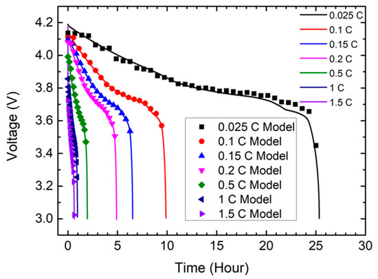
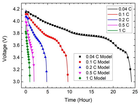
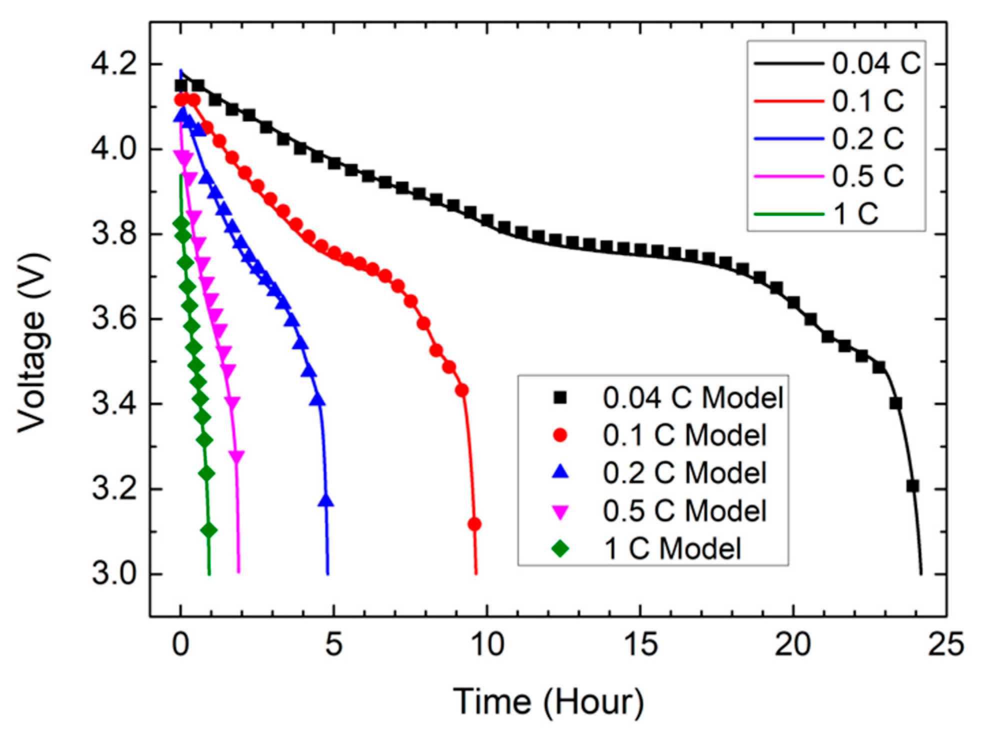
A total of 18,650 commercial lithium-ion cylindrical batteries were discharged with different C numbers of constant current. The L brand and S brand used 0.04 C, 0.1 C, 0.2 C, 0.5 C, and 1 C, respectively, with five different ways to discharge. The P brand used 0.025 C, 0.1 C, 0.15 C, 0.2 C, 0.5 C, 1 C, and 1.5 C to discharge in seven different ways. After the batteries were activated, we considered four batteries in series as one unit. Taking the L brand battery as an example, we first charged it with a constant current/voltage at 0.1 C to make the terminal voltage reach 16.8 V, then divided it into four batteries and discharged it with constant current from the terminal voltage of 4.2 V to 3 V. This was stopped when the discharge current dropped to 1/3 or 1/4, then we waited for 15 min before repeating this process 300 times, as shown in Figure 2.

Figure 2. Discharging flowchart (LOOP 300 times).

3.5. Multilayer Perceptron

Multilayer perceptron is a kind of forward pass neural network, which contains at least three layers (input layer, hidden layer, and output layer), and uses the technology of “backward propagation” to achieve supervised learning. In the current development of deep learning, MLP is actually a special case of a deep neural network. The recurrent neural network, long short-term memory, and gated recurrent unit concept are basically the same as MLP. Only DNN has more techniques and layers in the learning process, which will be greater and deeper. Therefore, our studies emphasized these three recurrent type deep neural networks and are described in the following section.

3.6. Recurrent Neural Network, Long Short Term Memory, and Gated Recurrent Unit

The simplest kind of neural network was introduced above, as multilayer neural networks (MLP). The output of each layer of calculation will only be forwarded to the input of the next layer in a single direction, that is to say, input and output are independent. One of the more advanced changes is the recurrent neural network (RNN). The difference between RNN and MLP is that RNN can pass the calculated output of a certain layer back to the layer itself as input. The output also becomes one of its own inputs at the next point in time (not another hidden layer). Therefore, there is memory in RNN. Because many application scenarios have the concept of sequence such as battery charge/discharge process (the probability of the next battery state depends on what the previous state is). Therefore, to train RNN, you need sequential data, where the input of RNN is the value of each variable in each time series. However, RNN has a shortcoming, that is, the earlier information has less influence on subsequent decision-making. When the time sequence passes, the influence of the previous information almost approaches zero. Therefore, we need a bit of a paradoxical network—long short term memory (LSTM). LSTM introduces three mechanisms to control memory, namely input gate, output gate, and forget gate. The changes in the opening and closing of these three gates have also become one of the variables. The machine learns to open or close by itself through data, thereby determining which information is the focus and which is noise. LSTM uses memory to enhance current decision-making, and uses three control gates to determine the storage and use of memory.

• In addition to the predicted output, a memory branch is added and updated over time. The current memory is represented by the “forget gate”, and “input gate” is used to determine whether to update the memory.
• Forget Gate: If the current sentence is a new topic or the opposite of the previous sentence, the previous sentence will be filtered out by this gate. Otherwise, it may continue to be retained in memory. This gate is usually a Sigmoid function.
• Input Gate: This determines whether the current input and the newly generated memory cell are added to the long term memory. This gate is also a Sigmoid function, which means that it needs to be added or not.
• Output Gate: This determines whether the current state is added to the output. This gate is also a Sigmoid function, indicating whether to add it or not.
• Finally, for whether the long-term memory is added to the output, the tanh function is usually used. The value of the output gate will fall between [−1, 1], and the −1 means removing the long-term memory.

LSTM also has the problem of slow execution speed, so the gated recurrent unit (GRU) was proposed to speed up execution and reduce memory consumption. The difference between GRU and LSTM is that GRU only uses two gates, namely the update gate and reset gate. The reset gate controls what percentage of the previous hidden state should be used to calculate the next hidden state with the new input. The update gate is to adjust the ratio of the hidden state to the previous hidden state to obtain the final hidden state.

3.7. Genetic Algorithm

Genetic algorithm (GA) [33,34,35,36,37] was proposed by Professor John Holland and his students around the 1970s and has been widely used to obtain the best results. It is used for optimization problems, artificial intelligence, data retrieval, machine learning, and deep learning. It is said to be a calculation method that simulates the evolution of natural organisms as various species will compete with each other in the environment and only the fittest will be able to survive.

There are some commonly used terms and concepts in genetic algorithms. The population is composed of several different individuals. Individuals are composed of genes and genes are the basic elements of forming chromosomes. A generation refers to the process of evolution. Holland believes that the process of natural evolution occurs within the genes of chromosomes. Evolution refers to the changes that occur in each generation of organisms. The characteristics of each organism are the genes of the previous generation, which determine the level of fitness. Therefore, the principle of survival of the fittest will leave the excellent genes behind and weed out the unsuitable ones. The evolutionary processes of these simulated organisms include reproduction, crossover, and mutation.

Crossover is the most important operation method in genetic algorithms. The process of evolution in the biological world may take tens of thousands of years, but it only takes a few seconds or minutes to use machines to execute genetic algorithms. If you want to obtain strong offspring, you must choose different genes for mating. The common selection methods are roulette wheel selection and tournament selection.

The roulette-style selection method is that each generation of individuals represents a block on the roulette. The size of the block is proportional to the fitness value of the individual. The two selected individuals will be sent to the mating pool for mating to obtain excellent offspring.

For competitive selection, two or more individuals are selected and the individual with a higher fitness value will be sent to the mating pool to wait. In the mating process, two chromosomes are used to produce offspring with some parent-like characteristics. The goal of mating is that the offspring have highly adapted chromosomes. However, it is also possible to inherit the shortcomings of the parents and the mating may not produce better offspring. After eliminating the offspring with shortcomings, an excellent offspring can continue to survive.

The mutation process will make random changes to the chromosomes. The common method will change a certain gene in the chromosome. The purpose of mutation is to let the genetic algorithm search for genes that have not appeared before and bring new genes into the population. However, too many mutations will destroy the structure of the genetic algorithm and cause the offspring to be quite different from their parents. If the number of mutations is too small, the offspring and their parents will not change in any way, so mutations will be regarded as a secondary calculation method.

4. Experiment Result

4.1. Manual Extraction Parameters

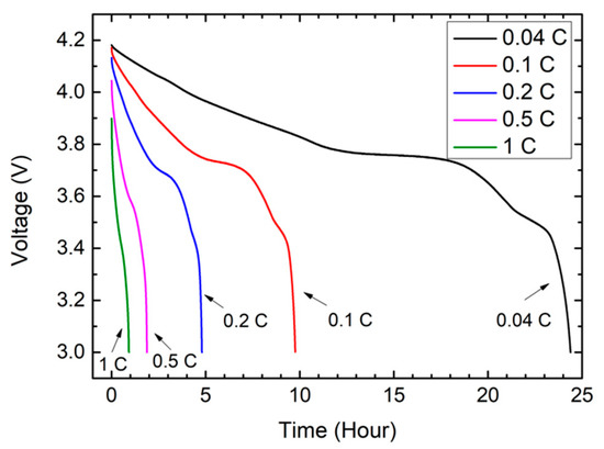
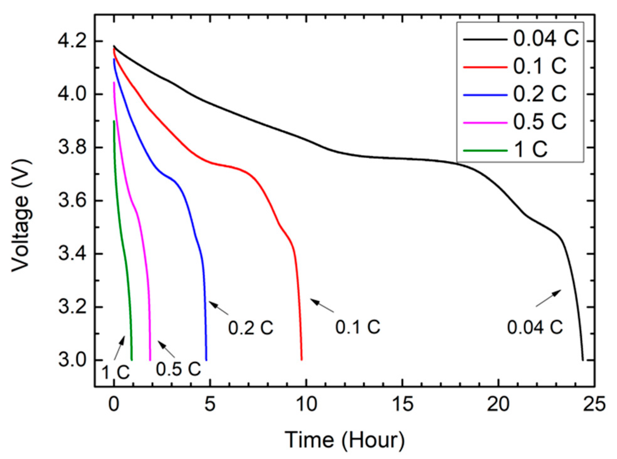
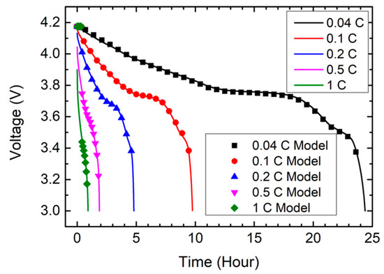
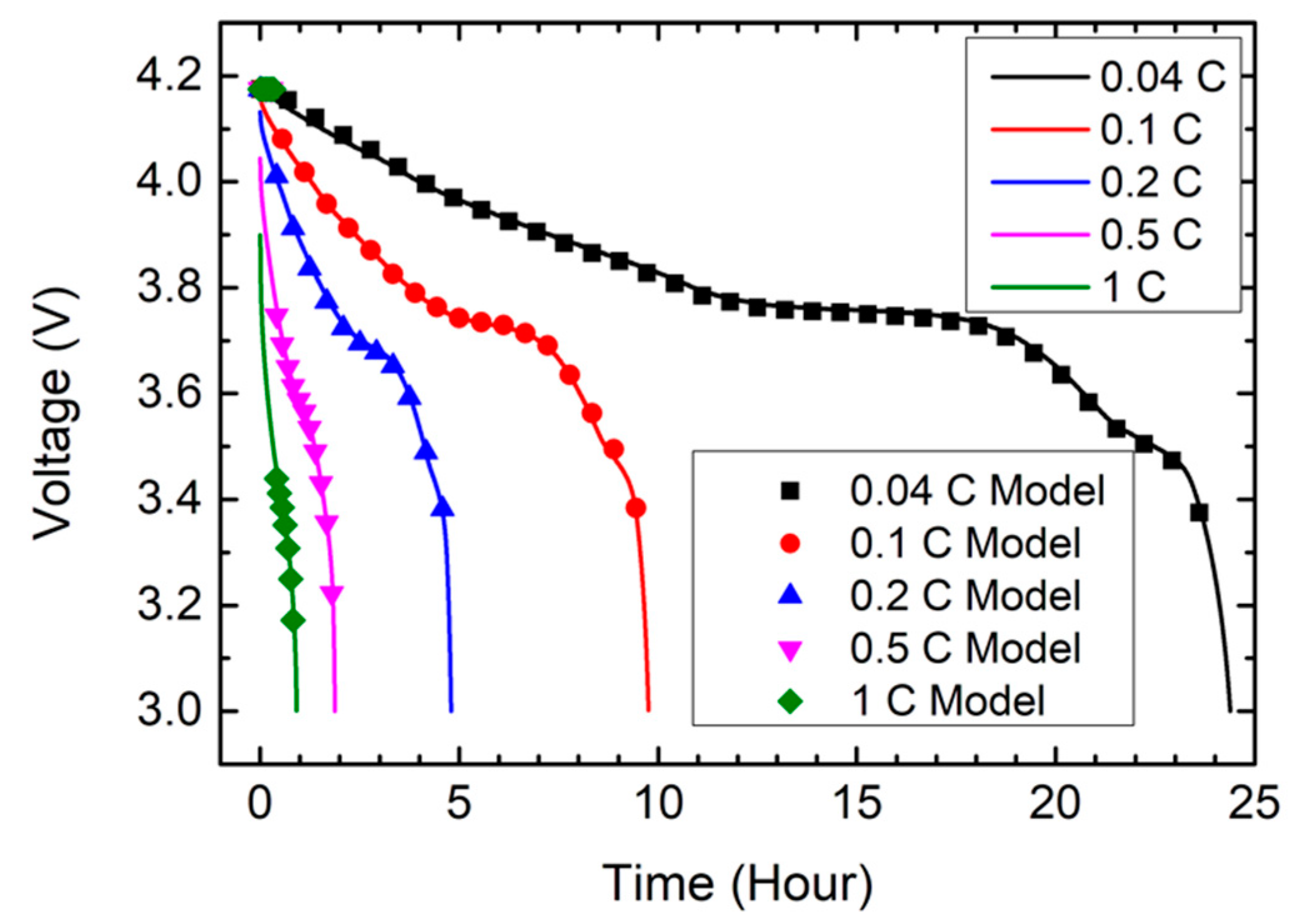
Before starting the experiment, we needed to know the discharge characteristic curve of the battery. Taking L brand 18650 as an example, Figure 3 shows the voltage curve of the battery under different discharge rates using a battery measuring instrument. From the viewpoint of energy conservation, the discharge time is shorter before the higher discharge rate reaches the discharge cut-off voltage, which is a normal phenomenon.

Figure 3. Discharge curve of L brand 18650.

The following equation employs three series subcells to describe the discharge characteristics of 18,650 commercial lithium-ion cylindrical batteries [4,38], where Vo1, Vo2, Vo3, Vc, Vk, I, K, τ1, τ2, τ3, τ4, and τ5 are the open-circuit voltage of subcell 1 to subcell 3, open-circuit voltage of batteries, voltage drop of external resistance, discharge current, decline constant of internal resistance, time constant 1 to 5, respectively.

(1)

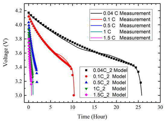
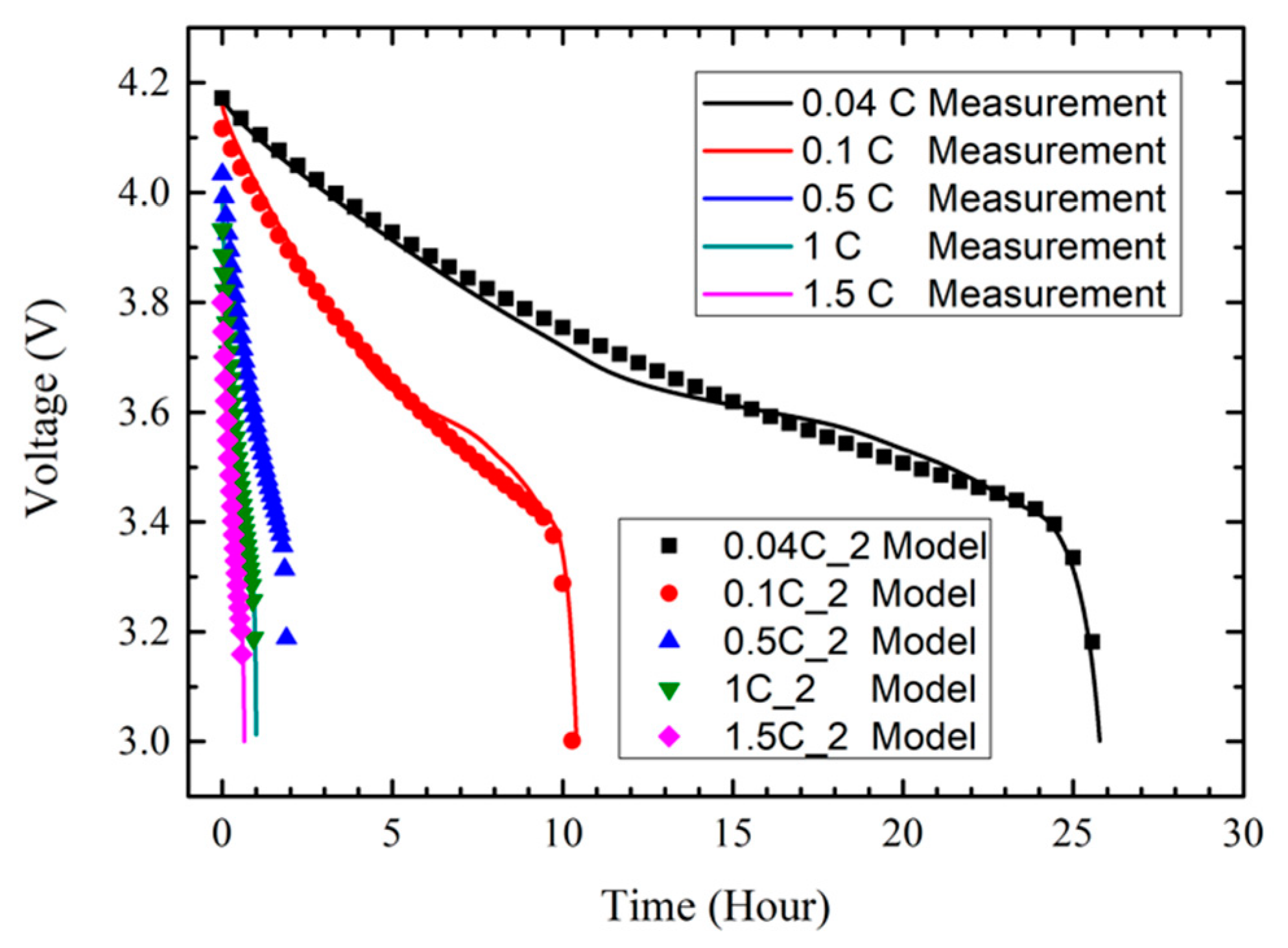
Using the discharge characteristic equation, we can find Figure 4 by manually extracting the parameters. Model is the original parameter and measurement is the value obtained from the manual extraction parameter. As shown in Figure 4, the manual extraction parameters differed from the original data. Considering the time cost, different algorithms were used to solve this problem.

Figure 4. Measurement of L brand 18650.

We used the root mean square error equation (RMSE) to express the training score where a smaller value is better.

4.2. MLP Result

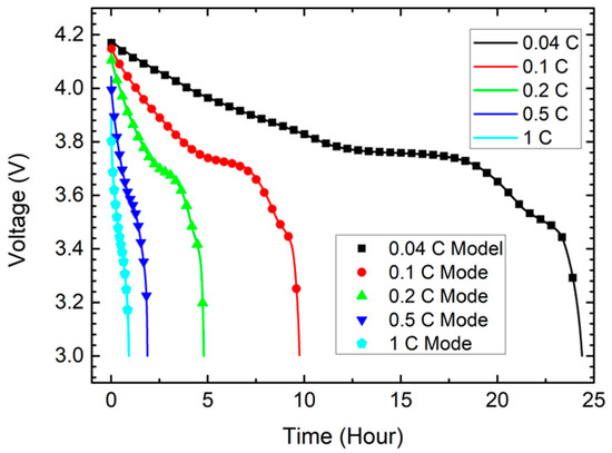
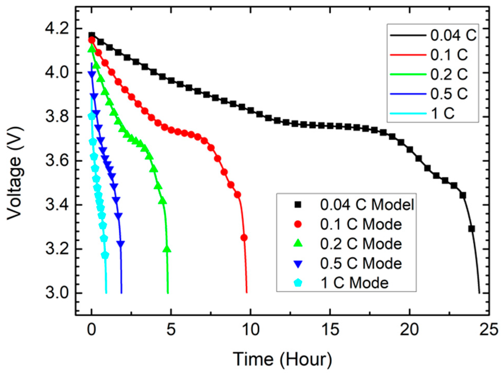
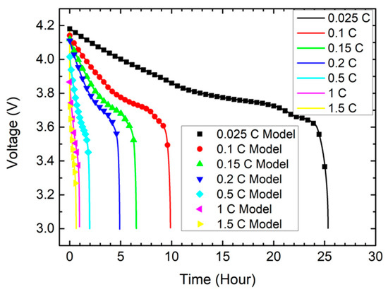
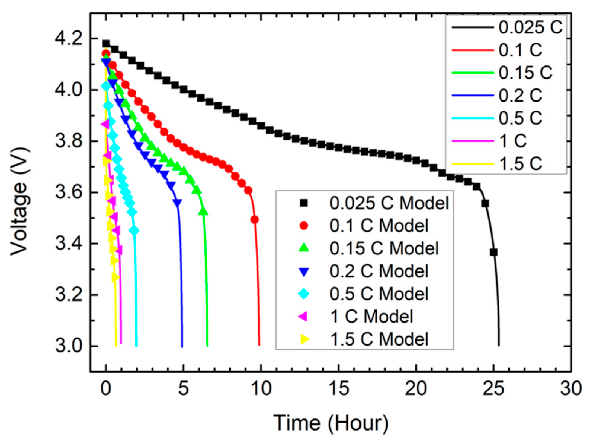
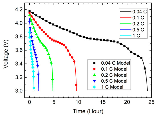
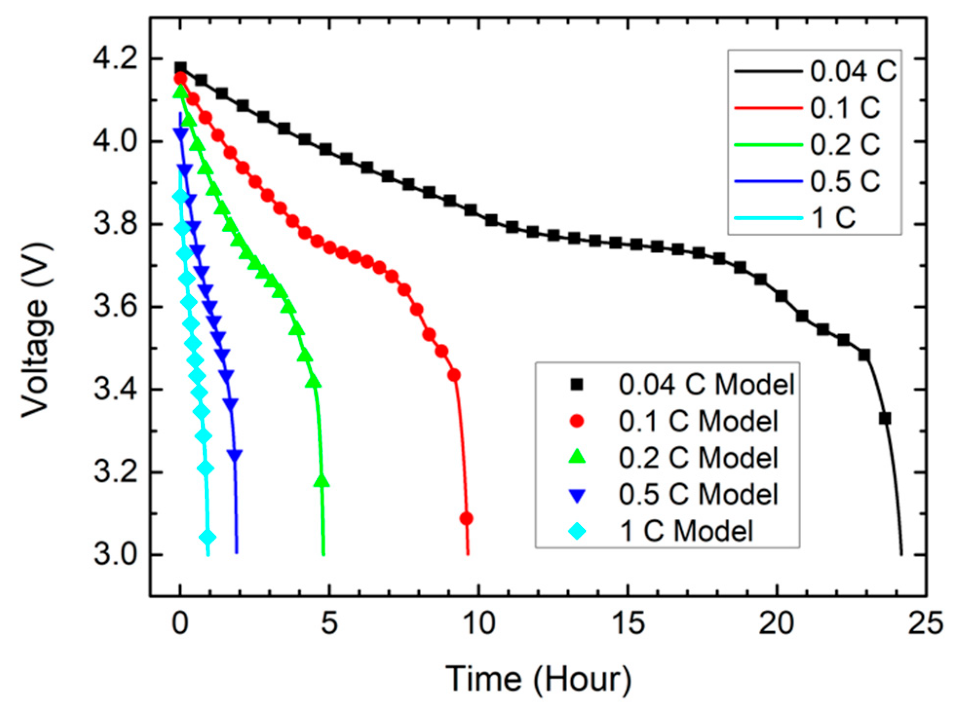
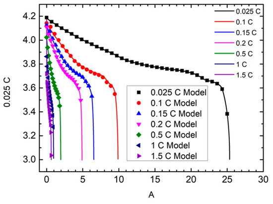
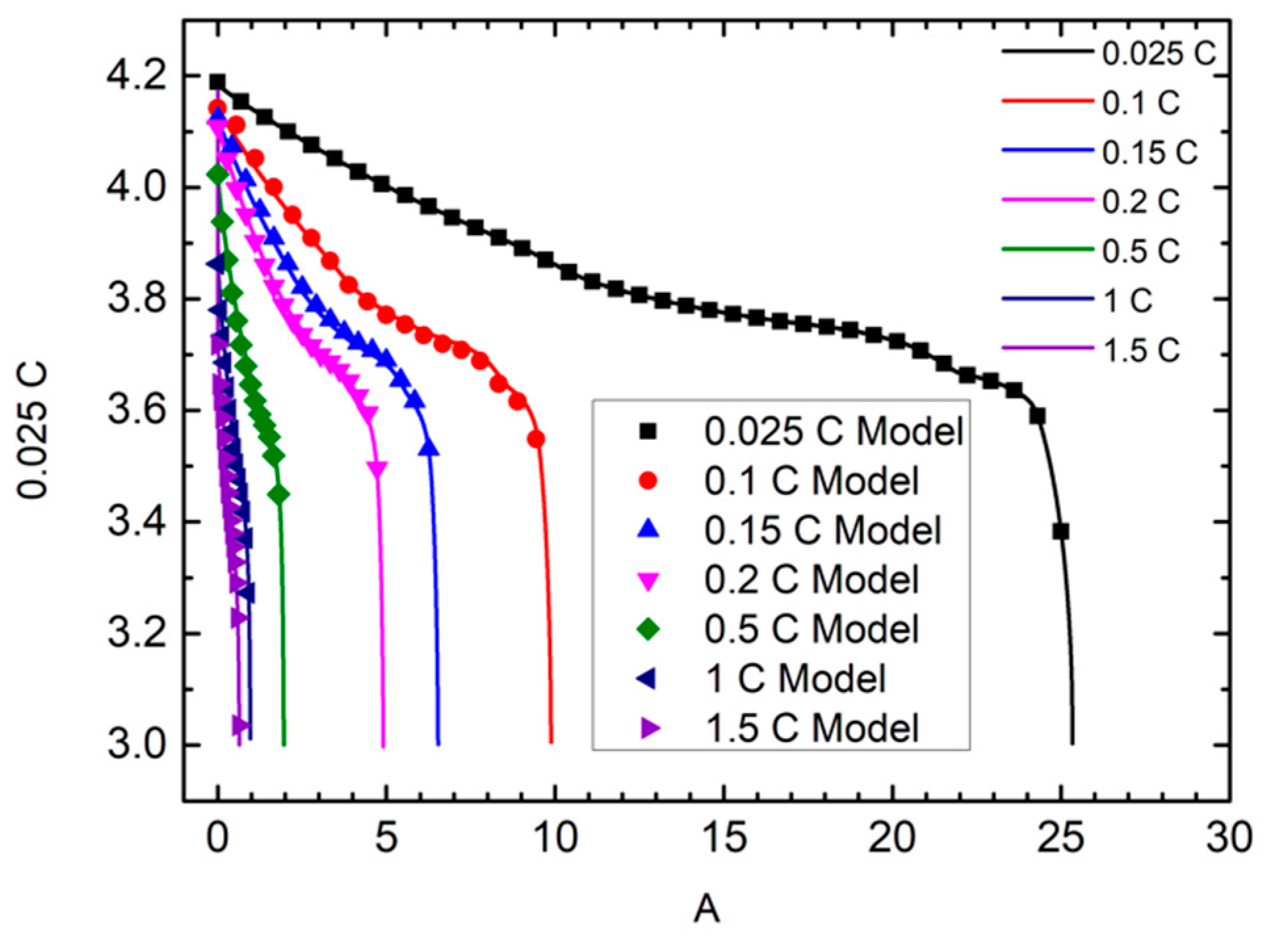
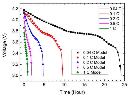
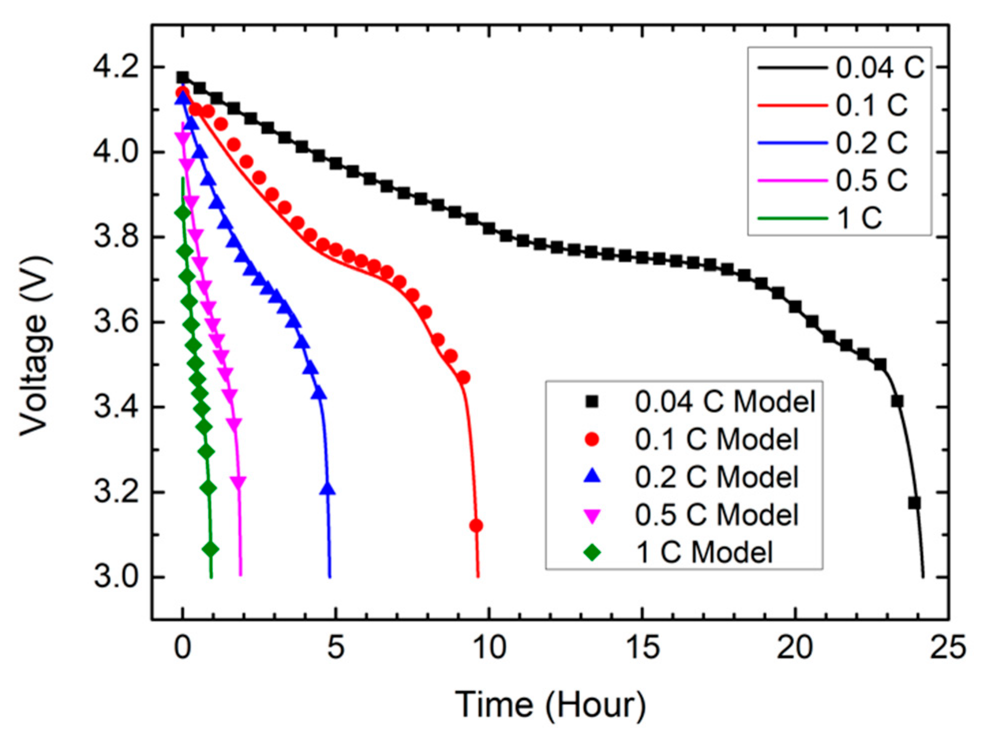
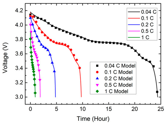
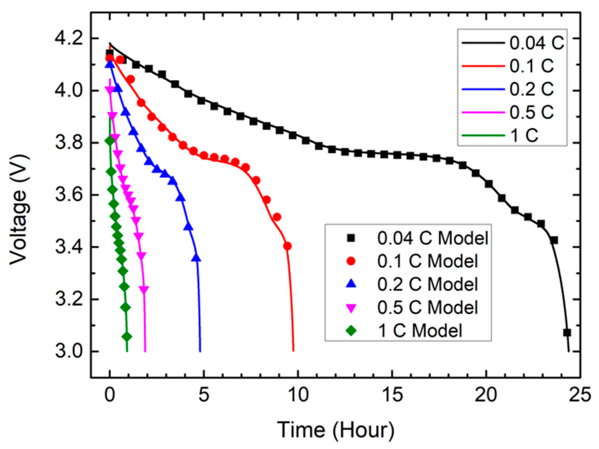
Figure 5, Figure 6 and Figure 7 show the measurement data of the L brand, P brand, and S brand batteries with varying discharging current: Epoch = 100, look_back = 10; model is the training data.

Figure 5. Curve of L brand 18650, Epoch = 100, look_back = 10.

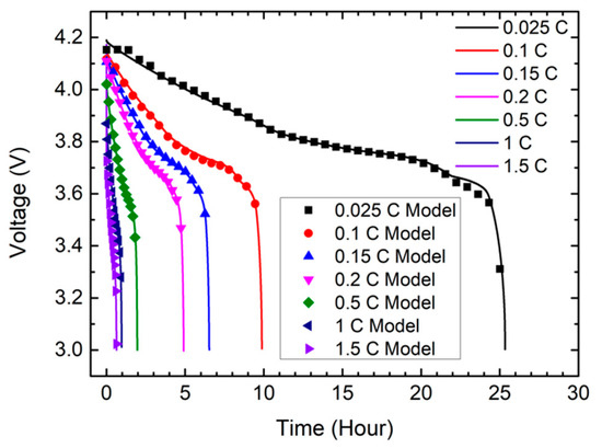
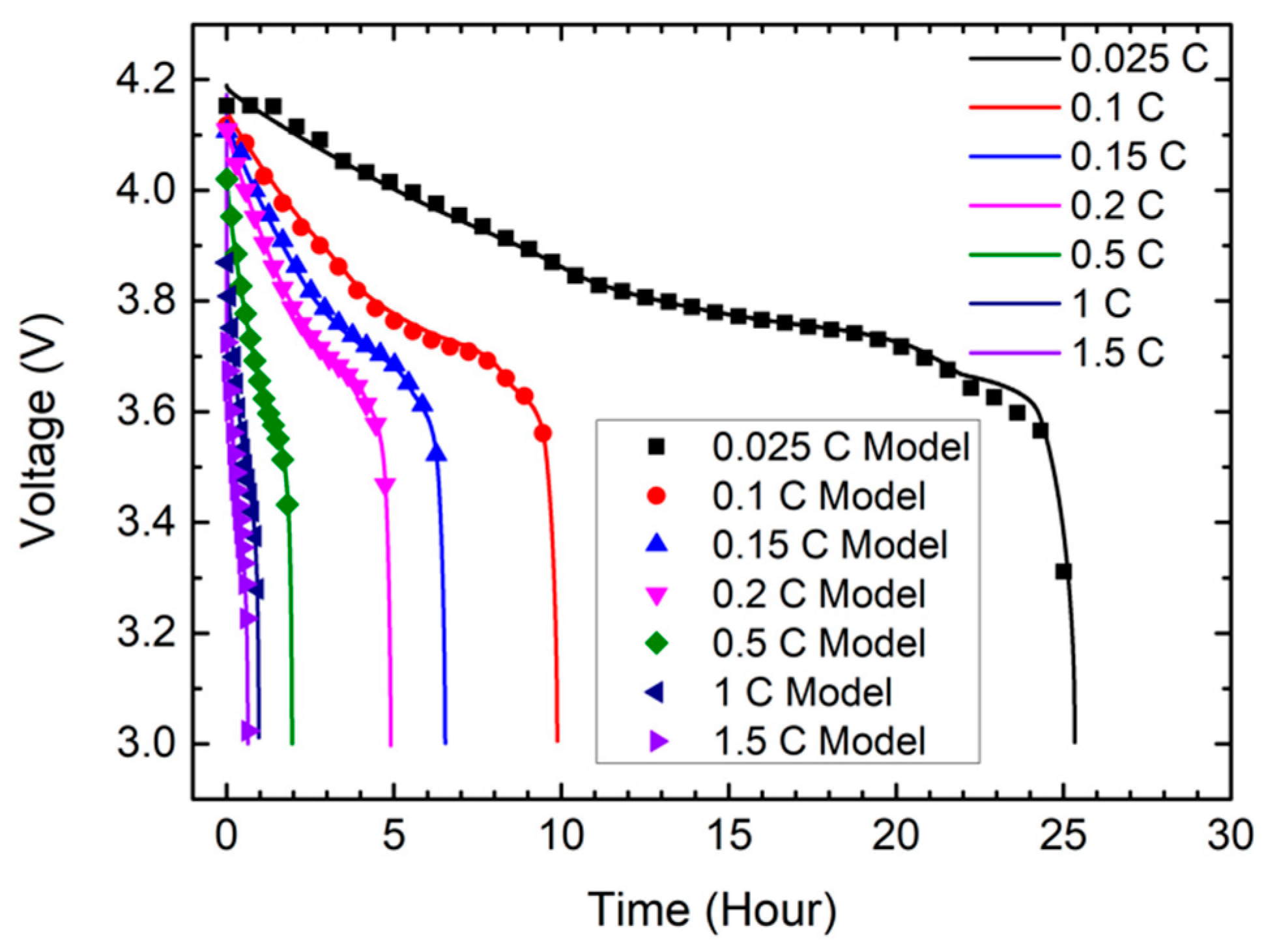
Figure 6. Curve of P brand 18650, Epoch = 100, look_back = 10.

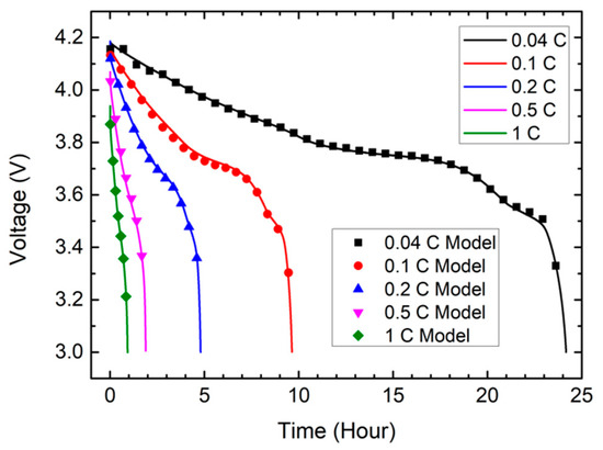
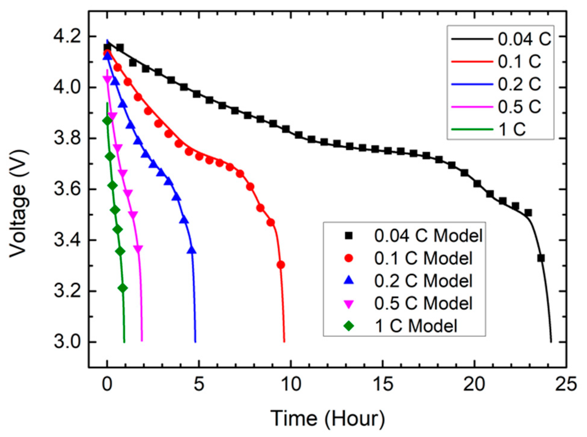
Figure 7. Curve of S brand 18650, Epoch = 100, look_back = 10.

Table 2 shows the score after the completion of training for Epoch = 100 and look_back = 10.

Table 2. Results of MLP, Epoch = 100, look_back = 10.

L Brand 18650	Score	P Brand 18650	Score	S Brand 18650	Score
C1E100LB10	2.3962	C1E100LB10	1.9665	C1E100LB10	1.416
C2E100LB10	1.0355	C2E100LB10	2.5641	C2E100LB10	5.1457
C3E100LB10	1.9235	C3E100LB10	2.1702	C3E100LB10	1.4973
C4E100LB10	2.5563	C4E100LB10	1.2151	C4E100LB10	1.9197
C5E100LB10	1.8657	C5E100LB10	3.4141	C5E100LB10	2.2744
		C6E100LB10	2.1928
		C7E100LB10	1.8609

4.3. RNN Result

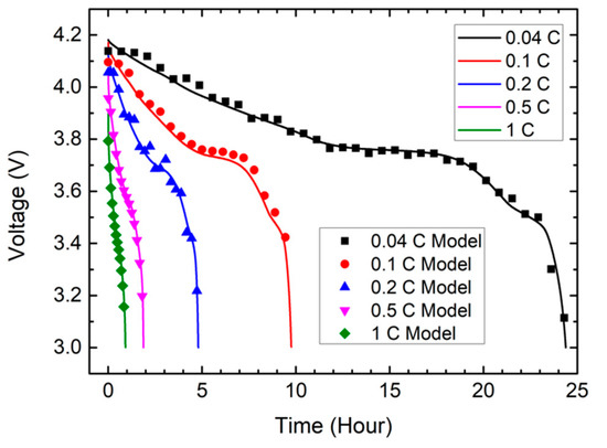
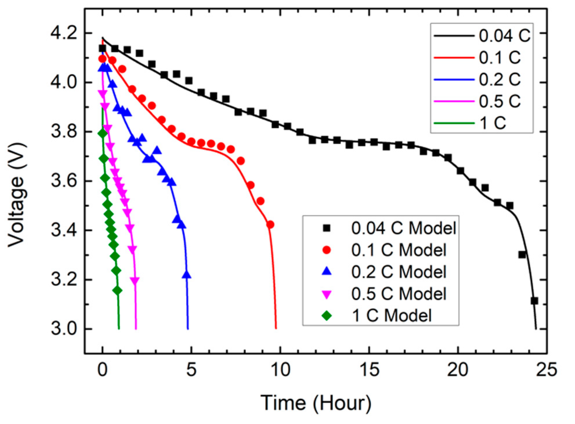
Figure 8, Figure 9 and Figure 10 show the measurement data of the L brand, P brand, and S brand batteries with varying discharging current: Epoch = 100, look_back = 10; model is the training data.

Figure 8. Curve of L brand 18650, Epoch = 100, look_back = 10.

Figure 9. Curve of P brand 18650, Epoch = 100, look_back = 10.

Figure 10. Curve of S brand 18650, Epoch = 100, look_back = 10.

Table 3 shows the score after the completion of training for Epoch = 100 and look_back = 10.

Table 3. Results of RNN, Epoch = 100, look_back = 10.

L Brand 18650	Score	P Brand 18650	Score	S Brand 18650	Score
C1E100LB10	22.7628	C1E100LB10	26.1699	C1E100LB10	10.2164
C2E100LB10	12.8867	C2E100LB10	15.3611	C2E100LB10	11.8313
C3E100LB10	19.2566	C3E100LB10	7.8641	C3E100LB10	16.3885
C4E100LB10	16.4656	C4E100LB10	13.1751	C4E100LB10	47.0949
C5E100LB10	14.4838	C5E100LB10	27.3929	C5E100LB10	23.4548
		C6E100LB10	12.1015
		C7E100LB10	11.0649

4.4. LSTM Result

Figure 11, Figure 12 and Figure 13 show the measurement data of the L brand, P brand, and S brand batteries with varying discharging current: Epoch = 100, look_back = 10; model is the training data.

Figure 11. Curve of L brand 18650, Epoch = 100, look_back = 10.

Figure 12. Curve of P brand 18650, Epoch = 150, look_back = 20.

Figure 13. Curve of S brand 18650, Epoch = 100, look_back = 10.

Table 4 shows the score after the completion of training for Epoch = 100 and look_back = 10.

Table 4. Results of LSTM, Epoch = 100, look_back = 10.

L Brand 18650	Score	P Brand 18650	Score	S Brand 18650	Score
C1E100LB10	35.2445	C1E100LB10	5.3272	C1E100LB10	5.2539
C2E100LB10	34.7757	C2E100LB10	7.2181	C2E100LB10	30.271
C3E100LB10	16.183	C3E100LB10	9.3963	C3E100LB10	8.6395
C4E100LB10	4.7719	C4E100LB10	3.2441	C4E100LB10	16.1969
C5E100LB10	7.4273	C5E100LB10	7.3323	C5E100LB10	11.1258
		C6E100LB10	5.8578
		C7E100LB10	3.7878

4.5. GRU Result

Figure 14, Figure 15 and Figure 16 show the measurement data of the L brand, P brand, and S brand batteries with varying discharging current: Epoch = 100, look_back = 10; model is the training data.

Figure 14. Curve of L brand 18650, Epoch = 100, look_back = 10.

Figure 15. Curve of P brand 18650, Epoch = 100, look_back = 10.

Figure 16. Curve of S brand 18650, Epoch = 100, look_back = 10.

Table 5 shows the score after the completion of training for Epoch = 100 and look_back = 10.

Table 5. Results of GRU, Epoch = 100, look_back = 10.

L Brand 18650	Score	P Brand 18650	Score	S Brand 18650	Score
C1E100LB10	11.7349	C1E100LB10	13.9564	C1E100LB10	7.9086
C2E100LB10	22.561	C2E100LB10	10.8346	C2E100LB10	14.9015
C3E100LB10	15.0054	C3E100LB10	8.2631	C3E100LB10	7.614
C4E100LB10	5.245	C4E100LB10	5.8903	C4E100LB10	21.8592
C5E100LB10	5.2089	C5E100LB10	12.3002	C5E100LB10	8.8804
		C6E100LB10	7.3077
		C7E100LB10	5.1895

4.6. GA Results

4.6.1. L Brand 18650

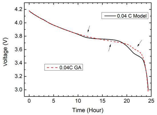
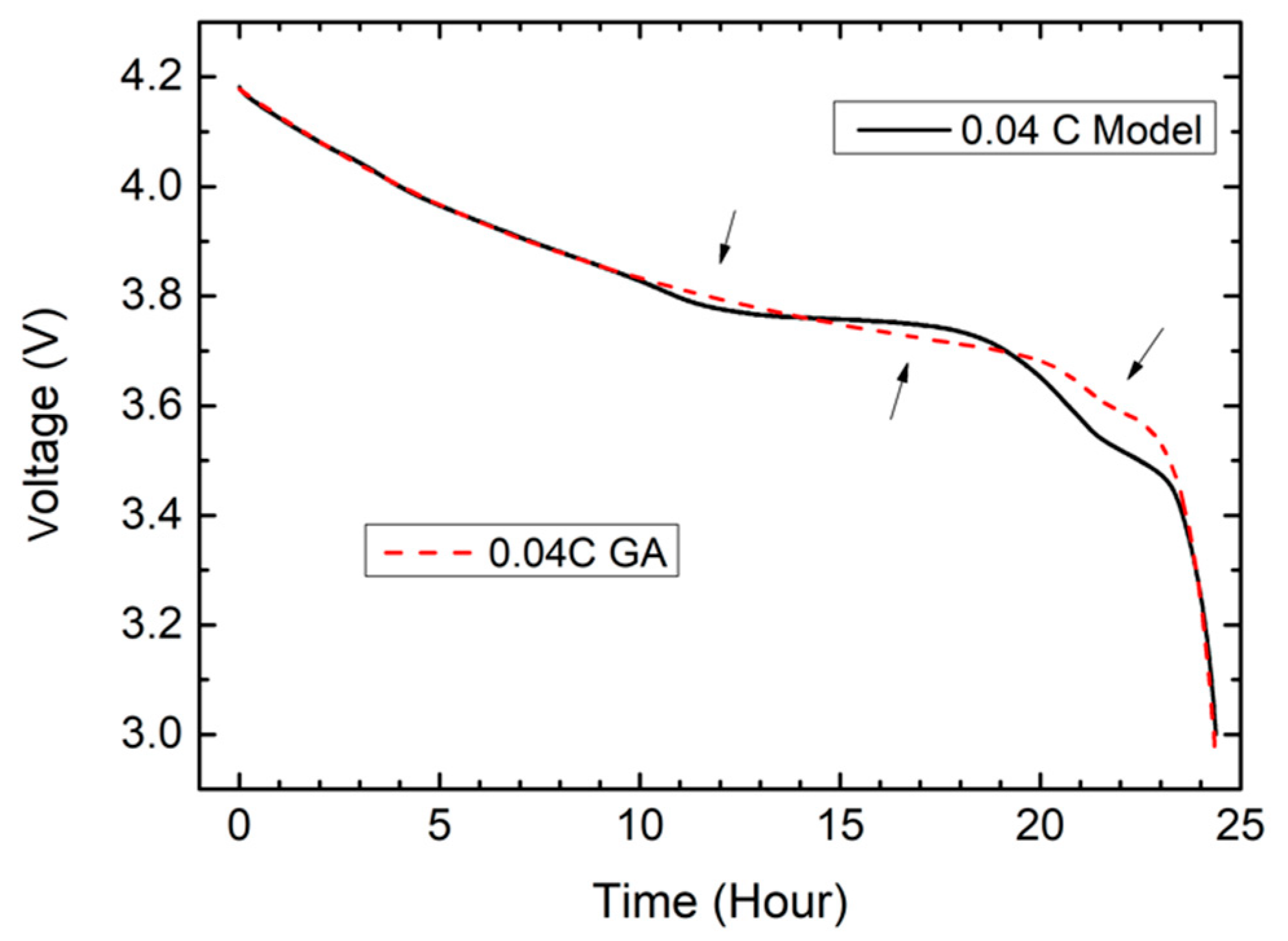
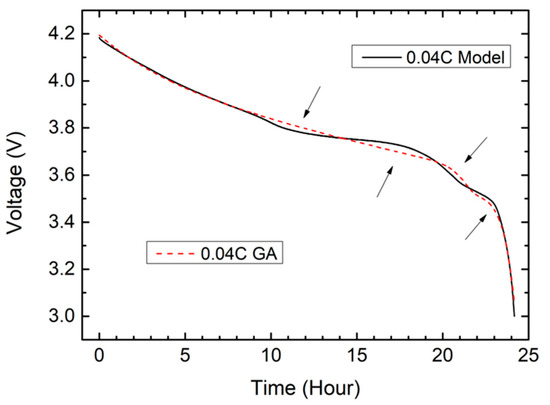
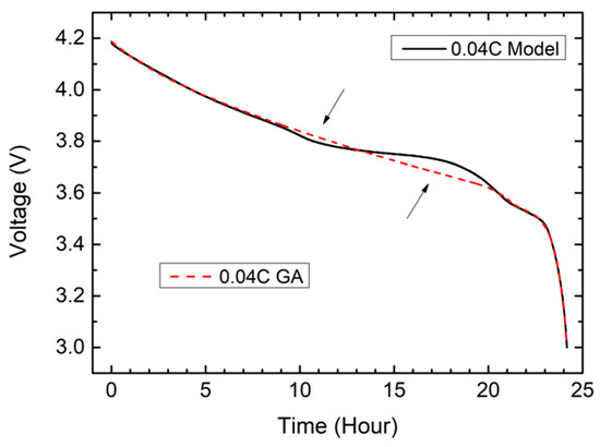
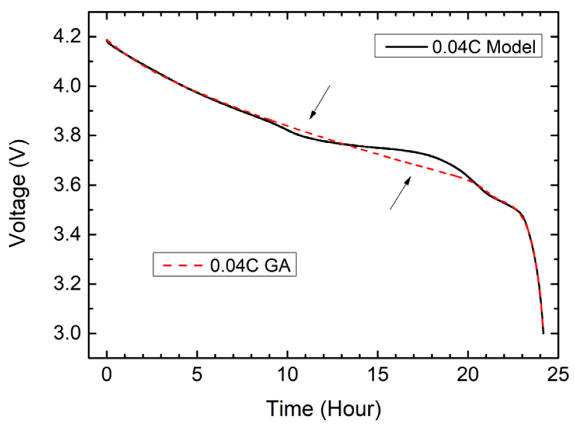
Figure 17 shows the results of L brand 18650 training with genetic algorithm (GA). The arrow points to the location where improvement is needed.

Figure 17. GA results (L brand 18650).

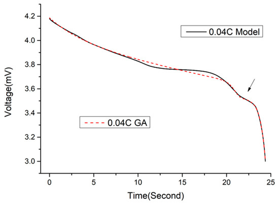
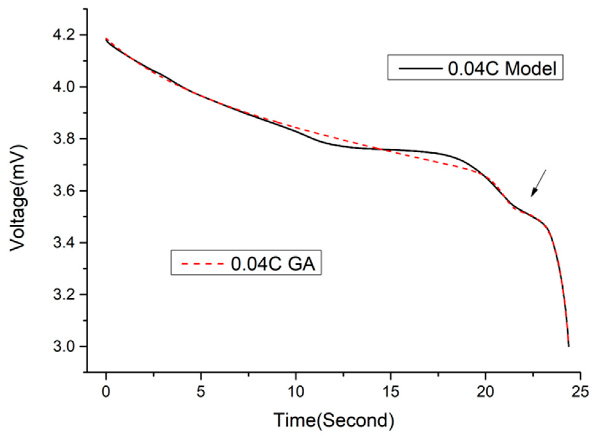
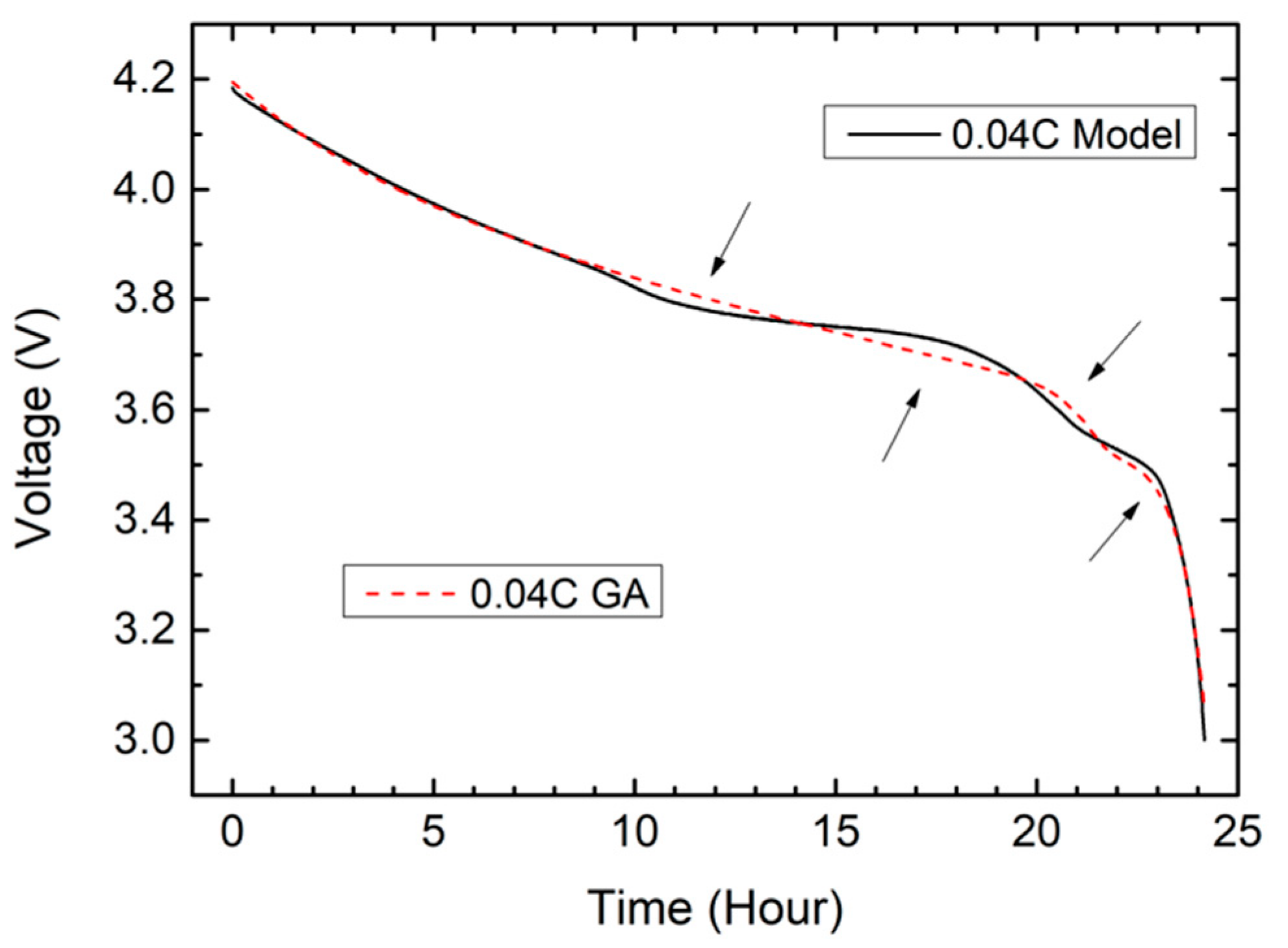
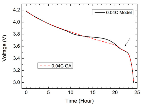
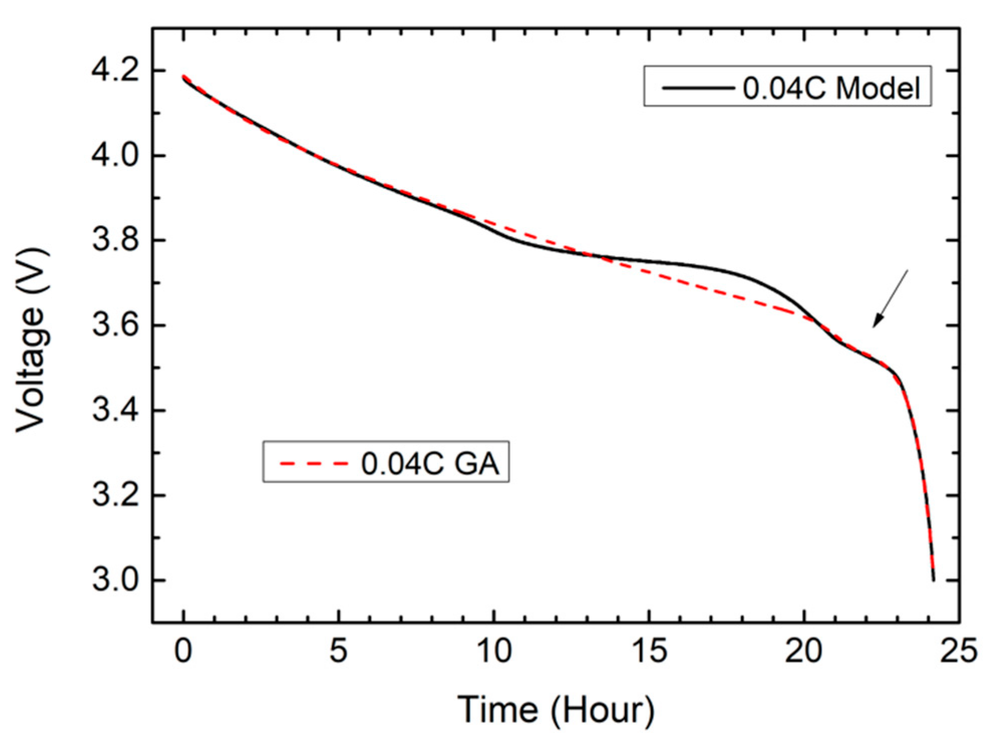
Figure 18 utilizes the improved data. The arrow in Figure 18 is consistent with that in Figure 17, and the arrow in Figure 19 is narrower than that in Figure 17. We added an extra capacitor to the discharge characteristic curve equation and increased the mutation rate and mating rate to make it easier for the program to find approximate values. Table 6 shows the parameters of GA for L brand 18650.

Figure 18. GA results 2 (L brand 18650).

Figure 19. GA results 2 (L brand 18650): reduce the range at the arrow.

Table 6. The parameters of GA (L brand 18650).

Parameter	Range	True Value
I	0.01~110	72.6875
K	1.4 × 10−13~1.4 × 10−19	1.3633 × 10−13
Vk	0~4000	3674
Vc	0~42,000	1292
Vo1	0~3000	2404
Vo2	0~35,000	10,603
Vo3	0~4000	2555
Vo4	0~70,000	30,444
τ1	0~140,000	5339
τ2	0~450,000,000	113,874,966
τ3	0~187,000	55,007
τ4	0~170,000	81,575
τ5	0~10,000	604
τ6	0~900,000,000	195,378,993

4.6.2. P Brand 18650

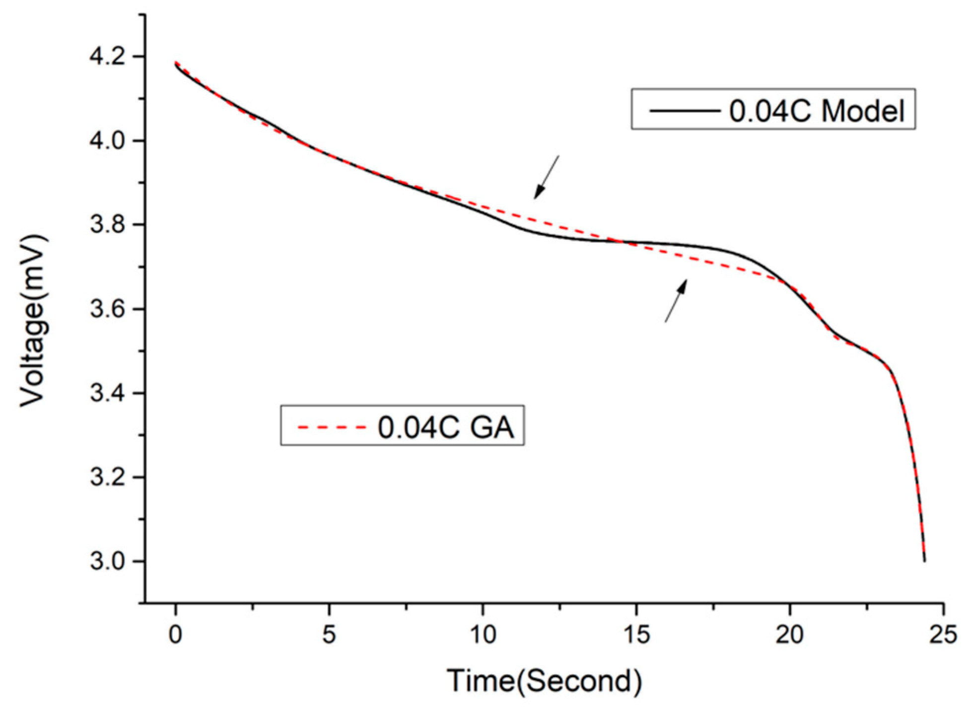
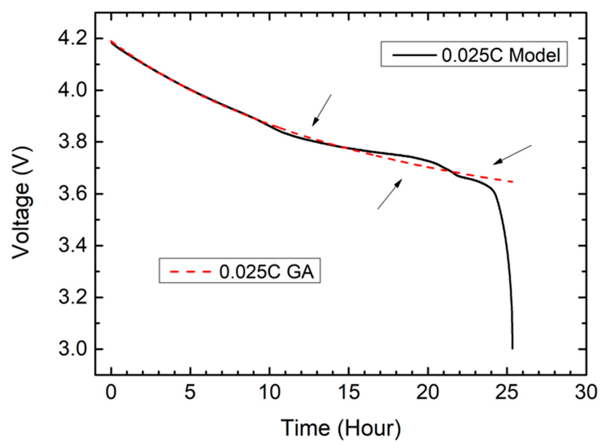
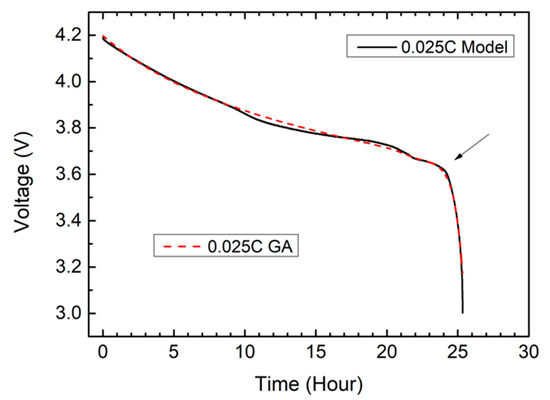
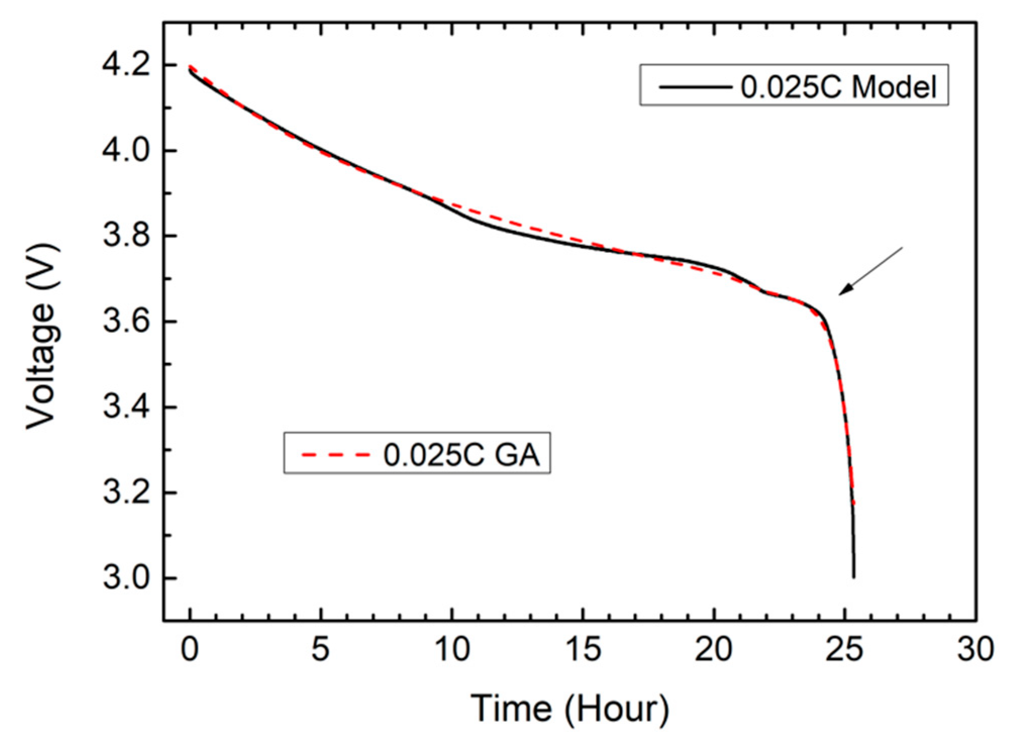
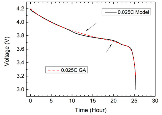
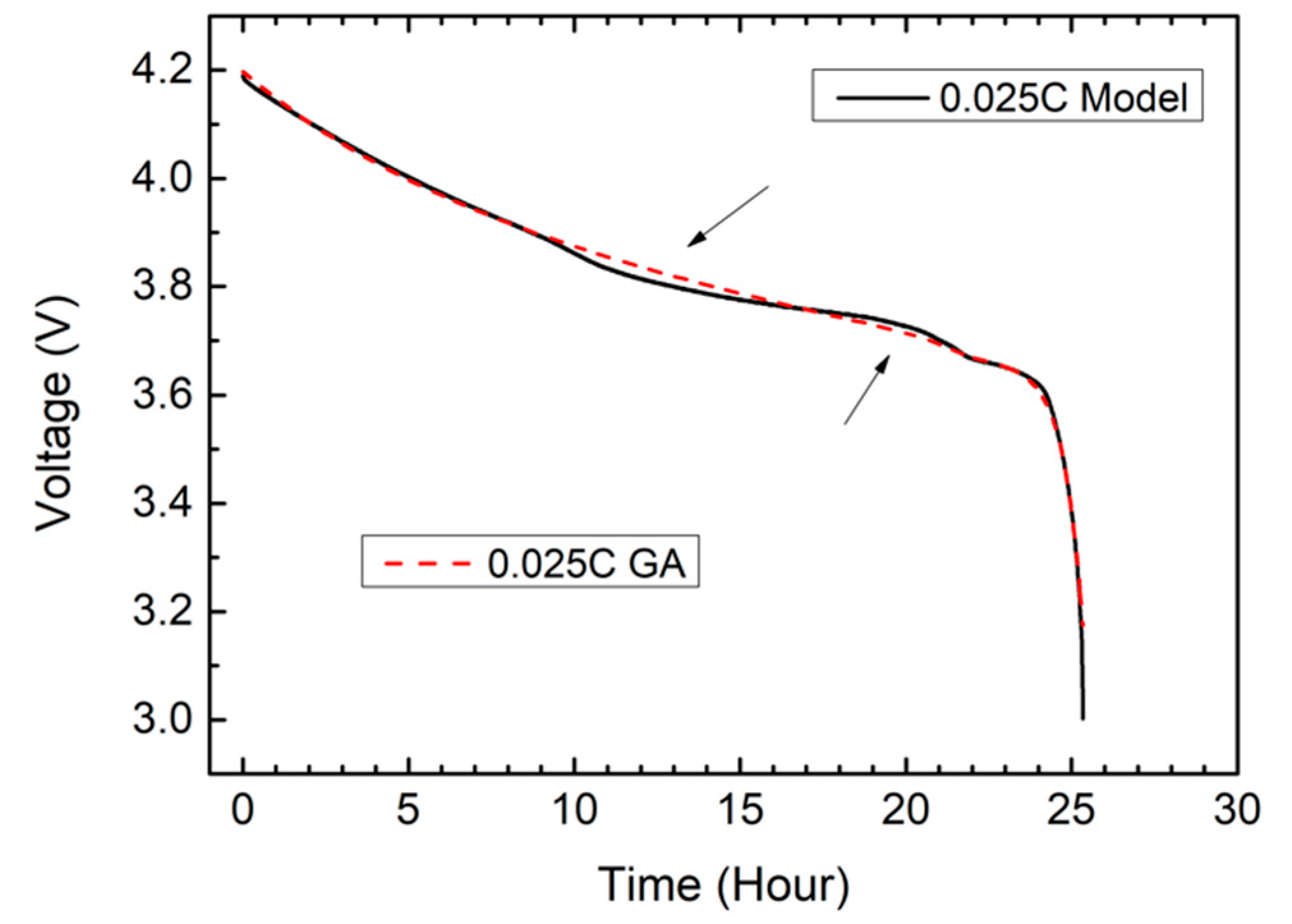
Figure 20 is the result of P brand 18650 training with genetic algorithm (GA). The arrow points to the locations where improvement is needed.

Figure 20. GA results (P brand 18650).

Figure 21 represents the improved data. The arrow in Figure 20 is significantly consistent with that in Figure 21. The arrow in Figure 22 is narrower than that in Figure 20. We added two more capacitors to the discharge characteristic curve equation and increased the mutation rate and mating rate to make it easier for the program to find approximate values. Table 7 shows the parameters of GA for P brand 18650.

Figure 21. GA results 2 (P brand 18650).

Figure 22. GA results 2 (P brand 18650): reduce the range at the arrow.

Table 7. The parameters of GA (P brand 18650).

Parameter	Range	True Value
I	0.01~110	76.8125
K	1.4 × 10−13~1.4 × 10−19	9.1103 × 10−14
Vk	0~4000	2941
Vc	0~42,000	1087
Vo1	0~3000	697
Vo2	0~35,000	9232
Vo3	0~4000	3554
Vo4	0~70,000	8213
Vo5	0~70,000	34247
τ1	0~140,000	35186
τ2	0~450,000,000	151,985,257
τ3	0~187,000	7117
τ4	0~170,000	87,017
τ5	0~10,000	651
τ6	0~900,000,000	155,079,888
τ7	0~900,000,000	712,175,902

4.6.3. S Brand 18650

Figure 23 shows the results of S-brand 18650 training with genetic algorithm (GA). The arrow marks the points where improvement is needed.

Figure 23. GA results (S brand 18650).

Figure 24 shows the improved data. The arrow in Figure 24 is consistent with that in Figure 23 and the arrow in Figure 25 is narrower than that in Figure 23. We added two more capacitors to the discharge characteristic curve equation and increased the mutation rate and mating rate to make it easier for the program to find approximate values. Table 8 shows the parameters of GA for S brand 18650.

Figure 24. GA results 2 (S brand 18650).

Figure 25. GA results 2 (S brand 18650): reduce the range at the arrow.

Table 8. The parameters of GA (S brand 18650).

Parameter	Range	True Value
I	0.01~110	82.75
K	1.4 × 10−13~1.4 × 10−19	1.3061 × 10−13
Vk	0~4000	2965
Vc	0~42,000	1144
Vo1	0~3000	2456
Vo2	0~35,000	33,368
Vo3	0~4000	2632
Vo4	0~70,000	52,797
Vo5	0~70,000	27,897
τ1	0~140,000	139,951
τ2	0~450,000,000	210,499,733
τ3	0~187,000	2942
τ4	0~170,000	47,774
τ5	0~10,000	671
τ6	0~900,000,000	818,734,152
τ7	0~900,000,000	457,604,887

5. Discussion

From the data, it is evident that the training result will have a similar curve to the output. By a simple lookup of the table, the data at different times, voltages, and currents can be found. However, for the values of time parameters and temperature, we cannot use these four methods.

To obtain all the parameter values that make up the equation and to solve this problem, we chose to use the genetic algorithm (GA). This method can set the parameters and range that are required to be solved. The program can imitate the natural world’s “survival of the fittest” and the rule of “elimination” to screen data.

In Table 3, Table 4 and Table 5, we can find the scores (RMSE) between different three recurrent-type model such as RNN, LSTM, and GRU. The average scores of LSTM were better than those of RNN and GRU, and the average of RNN was the worst score. However, we could also find the cure fitting type of Figure 8, Figure 9, Figure 10, Figure 11, Figure 12, Figure 13, Figure 14, Figure 15 and Figure 16. The LSTM cure was also estimated to describe the recurrent-type model more reliably. From Figure 17, Figure 18, Figure 19, Figure 20, Figure 21, Figure 22, Figure 23, Figure 24 and Figure 25, the predicted battery life of P brand 18650 was found as the GA parameters fit the battery life curve. However, S brand 18650 and L brand 18650 were not smooth discharge situations and their discharge situations in our study process were not always at thee down state. Therefore, as a whole, the battery discharge equation of the GA parameters is efficient to estimate the battery life.

6. Conclusions

In this paper, deep learning was used to describe the discharge characteristic curve of the battery. The discharge characteristic curve was used as the basis to establish the discharge model. The battery measuring instrument was used to charge and discharge the battery to establish the discharge characteristic curve.

First, we tried to find the discharge characteristic curve by manually extracting the parameters and found that the effect was not good and the time cost was huge. Therefore, MLP (multilayer perceptron), RNN (recurrent neural network), LSTM (long short-term memory), and GRU (gated recurrent unit) were used to improve this cost. The results obtained by these methods were graphs, but the requirement was to obtain the parameters of the discharge characteristic curve equation. Finally, we used the genetic algorithm (GA) to find the parameters of the discharge characteristic curve equation. This method can effectively find the parameter values that constitute the discharge characteristic curve equation.

References

- Ahuja, D.; Tatsutani, M. Sustainable energy for developing countries. Surv. Perspect. Integr. Environ. Soc. 2009, 2, 1. [Google Scholar]
- Pereira, J.C. Environmental issues and international relations, a new global (dis)order-the role of International Relations in promoting a concerted international system. Rev. Bras. Política Int. 2015, 58, 191–209. [Google Scholar] [CrossRef] [Scilit]
- Bryntesen, S.; Strømman, A.; Tolstorebrov, I.; Shearing, P.; Lamb, J.; Burheim, O.S. Opportunities for the State-of-the-Art Production of LIB Electrodes—A Review. Energies 2021, 14, 1406. [Google Scholar] [CrossRef] [Scilit]
- Piller, S.; Perrin, M.; Jossen, A. Methods for state-of-charge determination and their applications. J. Power Sources 2001, 96, 113–120. [Google Scholar] [CrossRef] [Scilit]
- Shen, Y.C. The Characteristics of Battery Discharge and Automodeling. Master Thesis, National Taiwan Ocean University, Keelung, Taiwan, 2013. [Google Scholar]
- Lee, S.J.; Kim, J.H.; Lee, J.M.; Cho, B.H. The State and Parameter Estimation of an Li-Ion Battery Using a New OCV-SOC Concept. In Proceedings of the Power Electronics Specialists Conference, Orlando, FL, USA, 17–21 June 2007; pp. 2799–2803. [Google Scholar]
- Ehret, C.; Piller, S.; Schroer, W.; Jossen, A. State-of-charge determination for lead-acid batteries in PV-applications. In Proceedings of the 16th European Photovoltaic Solar Energy Conference, Glasgow, UK, 1–5 May 2000. [Google Scholar]
- Huet, F. A review of impedance measurements for determination of the state-of-charge or state-of-health of secondary batteries. J. Power Sources 1998, 70, 59–69. [Google Scholar] [CrossRef] [Scilit]
- Yu, Z.; Huai, R.; Xiao, L. State-of-Charge Estimation for Lithium-Ion Batteries Using a Kalman Filter Based on Local Linearization. Energies 2015, 8, 7854–7873. [Google Scholar] [CrossRef] [Scilit]
- Chan, C.; Lo, E.; Weixiang, S. The available capacity computation model based on artificial neural network for lead–acid batteries in electric vehicles. J. Power Sources 2000, 87, 201–204. [Google Scholar] [CrossRef] [Scilit]
- Hsieh, Y.; Tan, S.; Gu, S.; Jeng, Y. Prediction of Battery Discharge States Based on the Recurrent Neural Network. J. Internet Technol. 2020, 21, 113–120. [Google Scholar]
- Hsieh, Y.-Z.; Lin, S.-S.; Luo, Y.-C.; Jeng, Y.-L.; Tan, S.-W.; Chen, C.-R.; Chiang, P.-Y.; Hsieh, Y.-Z.; Lin, S.-S.; Luo, Y.-C.; et al. ARCS-Assisted Teaching Robots Based on Anticipatory Computing and Emotional Big Data for Improving Sustainable Learning Efficiency and Motivation. Sustainability 2020, 12, 5605. [Google Scholar] [CrossRef] [Scilit]
- Shahrivar, E.M.; Sundaram, S. The Strategic Formation of Multi-Layer Networks. IEEE Trans. Netw. Sci. Eng. 2015, 2, 164–178. [Google Scholar] [CrossRef] [Scilit]
- Vilovic, I.; Burum, N. A comparison of MLP and RBF neural networks architectures for electromagnetic field prediction in indoor environments. In Proceedings of the 5th European Conference on Antennas and Propagation (EUCAP), Rome, Italy, 11–15 April 2011; pp. 1719–1723. [Google Scholar]
- Xiang, C.; Ding, S.Q.; Lee, T.H. Architecture analysis of MLP by geometrical interpretation. In Proceedings of the 2004 International Conference on Communications, Circuits and Systems (IEEE Cat. No.04EX914), Chengdu, China, 27–29 June 2004; Volume 2, pp. 1042–1046. [Google Scholar] [CrossRef] [Scilit]
- Xiang, C.; Ding, S.Q.; Lee, T.H. Geometrical Interpretation and Architecture Selection of MLP. IEEE Trans. Neural Netw. 2005, 16, 84–96. [Google Scholar] [CrossRef] [Scilit] [PubMed]
- Rumelhart, D.E.; Hinton, G.E.; Williams, R.J. Learning representations by back-propagating errors. Nature 1986, 323, 533–536. [Google Scholar] [CrossRef] [Scilit]
- Uçkun, F.A.; Özer, H.; Nurbaş, E.; Onat, E. Direction Finding Using Convolutional Neural Networks and Convolutional Recurrent Neural Networks. In Proceedings of the 2020 28th Signal Processing and Communications Applications Conference (SIU), Gaziantep, Turkey, 5–7 October 2020; pp. 1–4. [Google Scholar] [CrossRef] [Scilit]
- Boden, M.; Hawkins, J. Improved Access to Sequential Motifs: A Note on the Architectural Bias of Recurrent Networks. IEEE Trans. Neural Netw. 2005, 16, 491–494. [Google Scholar] [CrossRef] [PubMed]
- Sepp, H.; Jürgen, S. Long Short-Term Memory. Neural Comput. 1997, 9, 1735–1780. [Google Scholar]
- Heck, J.C.; Salem, F.M. Simplified minimal gated unit variations for recurrent neural networks. In Proceedings of the 2017 IEEE 60th International Midwest Symposium on Circuits and Systems (MWSCAS), Boston, MA, USA, 6–9 August 2017; pp. 1593–1596. [Google Scholar] [CrossRef] [Scilit]
- Kumar, B.P.; Hariharan, K. Multivariate Time Series Traffic Forecast with Long Short Term Memory based Deep Learning Model. In Proceedings of the 2020 International Conference on Power, Instrumentation, Control and Computing (PICC), Thrissur, India, 17–19 December 2020; pp. 1–5. [Google Scholar] [CrossRef] [Scilit]
- Sheikhfaal, S.; Demara, R.F. Short-Term Long-Term Compute-in-Memory Architecture: A Hybrid Spin/CMOS Approach Supporting Intrinsic Consolidation. IEEE J. Explor. Solid-State Comput. Devices Circuits 2020, 6, 62–70. [Google Scholar] [CrossRef] [Scilit]
- Schmidhuber, J.; Gers, F.; Eck, D. Learning Nonregular Languages: A Comparison of Simple Recurrent Networks and LSTM. Neural Comput. 2002, 14, 2039–2041. [Google Scholar] [CrossRef] [Scilit] [PubMed]
- Liu, B.; Meng, P. Hybrid Algorithm Combining Ant Colony Algorithm with Genetic Algorithm for Continuous Domain. In Proceedings of the 2008 The 9th International Conference for Young Computer Scientists, Hunan, China, 18–21 November 2008; pp. 1819–1824. [Google Scholar] [CrossRef] [Scilit]
- Apostolov, P.S.; Stefanov, A.K.; Bagasheva, M.S. Efficient FIR Filter Synthesis Using Sigmoidal Function. In Proceedings of the 2019 X National Conference with International Participation (ELECTRONICA), Sofia, Bulgaria, 16–17 May 2019; pp. 1–4. [Google Scholar] [CrossRef] [Scilit]
- Komatsuzaki, Y.; Otsuka, H.; Yamanaka, K.; Hamamatsu, Y.; Shirae, K.; Fukumoto, H. A low distortion Doherty amplifier by using tanh function gate bias control. In Proceedings of the 2014 Asia-Pacific Microwave Conference, Sendai, Japan, 4–7 November 2014; pp. 110–112. [Google Scholar]
- Junyoung, C.; Caglar, G.; KyungHyun, C.; Yoshua, B. Empirical Evaluation of Gated Recurrent Neural Networks on Sequence Modeling. arXiv 2014, arXiv:1412.3555. [Google Scholar]
- Turan, A.; Kayıkçıoğlu, T. Neuronal motifs of long term and short term memory functions. In Proceedings of the 2014 22nd Signal Processing and Communications Applications Conference (SIU), Trabzon, Turkey, 23–25 April 2014; pp. 1255–1258. [Google Scholar] [CrossRef] [Scilit]
- Mirza, A.H. Online additive updates with FFT-IFFT operator on the GRU neural networks. In Proceedings of the 2018 26th Signal Processing and Communications Applications Conference (SIU), Izmir, Turkey, 2–5 May 2018; pp. 1–4. [Google Scholar] [CrossRef] [Scilit]
- Mirza, A.H. Variants of combinations of additive and multiplicative updates for GRU neural networks. In Proceedings of the 2018 26th Signal Processing and Communications Applications Conference (SIU), Izmir, Turkey, 2–5 May 2018; pp. 1–4. [Google Scholar] [CrossRef] [Scilit]
- Yang, S.; Yu, X.; Zhou, Y. LSTM and GRU Neural Network Performance Comparison Study: Taking Yelp Review Dataset as an Example. In Proceedings of the 2020 International Workshop on Electronic Communication and Artificial Intelligence (IWECAI), Qingdao, China, 12–14 June 2020; pp. 98–101. [Google Scholar] [CrossRef] [Scilit]
- Pavithra, M.; Saruladha, K.; Sathyabama, K. GRU Based Deep Learning Model for Prognosis Prediction of Disease Progression. In Proceedings of the 2019 3rd International Conference on Computing Methodologies and Communication (ICCMC), Erode, India, 27–29 March 2019; pp. 840–844. [Google Scholar] [CrossRef] [Scilit]
- Yichen, L.; Bo, L.; Chenqian, Z.; Teng, M. Intelligent Frequency Assignment Algorithm Based on Hybrid Genetic Algorithm. In Proceedings of the 2020 International Conference on Computer Vision, Image and Deep Learning (CVIDL), Nanchang, China, 15–17 May 2020; pp. 461–467. [Google Scholar] [CrossRef] [Scilit]
- Jiang, J.; Butler, D. A genetic algorithm design for vector quantization. In Proceedings of the First International Conference on Genetic Algorithms in Engineering Systems: Innovations and Applications, Sheffield, UK, 12–14 September 1995; pp. 331–336. [Google Scholar] [CrossRef] [Scilit]
- Wang, J.; Hong, W.; Li, X. The Influence of Genetic Initial Algorithm on the Highest Likelihood in Gaussian Mixture Model. In Proceedings of the 2006 6th World Congress on Intelligent Control and Automation, Dalian, China, 21–23 June 2006; pp. 3580–3583. [Google Scholar] [CrossRef] [Scilit]
- Chen, M.; Yao, Z. Classification Techniques of Neural Networks Using Improved Genetic Algorithms. In Proceedings of the 2008 Second International Conference on Genetic and Evolutionary Computing, Jinzhou, China, 25–26 September 2008; pp. 115–119. [Google Scholar] [CrossRef] [Scilit]
- Ananda, S.; Lakshminarasamma, N.; Radhakrishna, V.; Srinivasan, M.S.; Satyanarayana, P.; Sankaran, M. Generic Lithium ion battery model for energy balance estimation in spacecraft. In Proceedings of the 2018 IEEE International Conference on Power Electronics, Drives and Energy Systems (PEDES), Chennai, India, 18–21 December 2018; pp. 1–5. [Google Scholar] [CrossRef] [Scilit]
Publisher’s Note: MDPI stays neutral with regard to jurisdictional claims in published maps and institutional affiliations. |
© 2021 by the authors. Licensee MDPI, Basel, Switzerland. This article is an open access article distributed under the terms and conditions of the Creative Commons Attribution (CC BY) license (https://creativecommons.org/licenses/by/4.0/).