1. Introduction
Due to the increasing number of renewable energy sources with a share in energy systems, research is being conducted on a large scale to increase conventional power plant flexibility [
1]. This aspect was addressed in [
2], where the authors analyzed increased flexibility in systems with a high share of renewable sources. In [
3], the flexibility and economic aspects of power plant operation in new low-carbon systems were analyzed. Increasing the flexibility of coal-fired power plant operation by activities related to the regulation of the steam cycle are presented in [
4]. In [
5,
6], the cooperation of conventional power plants was analyzed in terms of the power grid flexibility. The works mentioned here are broadly related to increasing the power range flexibility to lower the coal unit minimum load [
7]. At present, most coal-fired unit operating power fits the range of 50–100% of nominal capacity. In case of a significant power increase in the system due to the power produced by units with priority, e.g., renewables, the currently running conventional power plants reduce their operation [
8]. If the power supplied to the electricity network still exceeds the demand, some conventional units have to be shut down and prepared for restart [
9]. Shutting down and restarting coal-fired units is economically inefficient, shortens the unit’s lifetime, and causes increased emissions of harmful substances [
7]. Therefore, research to reduce the minimum power block output to values below 50% of the nominal load increases their stable operation under current conditions.
At the same time, the emission standards, concerning mainly dust, sulfur oxides, and nitrogen oxides emissions, have recently been stringent [
3]. Selective catalytic reduction (SCR) technology is the most frequently used for reducing nitrogen oxides in coal-fired power boilers, as indicated in [
10,
11]. Such installations require operation in a specific flue gas temperature range [
11], between 585 K and 670 K, depending on the catalyst type. The required range is also indicated in [
12] (the authors analyzed the installation and its impact on the quality of flue gases), and [
13] concerns the installation’s operation optimization. The issue that arises relatively often during attempts to increase the boiler operation flexibility is the insufficiently high flue gas temperature before the SCR installation, which results in its incorrect operation. One of the solutions for a too low temperature before the SCR issue is to connect the higher temperature flue gas from another part of the boiler to the main flue gas stream before the SCR installation. In the solution mentioned above, the key is to effectively mix the flue gas streams at different temperatures to obtain a uniform flue gas temperature field before the installation. The routing of an additional duct for transporting hot exhaust gases requires the consideration of design possibilities. In many modernized coal boilers, the SCR systems were installed additionally, so it is necessary to introduce hot flue gases from the top of the duct. There is a high risk of not mixing the hot flue gas stream with the main, cooler stream in such a configuration. The solution presented in this paper in the form of an adequately profiled turbulizing flap enables effective mixing of exhaust gas streams with the introduction of hot exhaust gas from the top of the duct and obtaining a temperature field with appropriate uniformity before the SCR installation.
If the elements regulating the flue gas flow installation, e.g., control vanes or flaps, are planned in an existing boiler, a key parameter that should be considered is the flue gas pressure drop caused by the installed element, especially in boiler operation with high loads. Any additional pressure drop in the flue gas ducts increases the flue gas fans’ power consumption, and in some cases, it can cause fan inefficiency. Increased power consumption also negatively affects the overall power unit efficiency. The technology developed by the authors makes it possible to regulate the pressure drop caused by the additional turbulence flap, with the possibility to fold the flap during the boiler operation with the nominal load. Thus, the impact of the device on the flue gas pressure drop is reduced to a minimum.
With the increasing availability of computational power, computational fluid dynamics (CFD) is increasingly being applied to the calculation of power boilers [
14,
15,
16,
17,
18], characterized by relatively large calculation volumes and multiple physical and chemical phenomena. CFD methods are used in power boiler calculations for many purposes. In [
15], the CFD method was used to optimize nitrogen oxide removal from exhaust gases. The temperature distribution in the boiler, validated by acoustic measurements, was modeled in [
16]. In several studies, the main objective was to determine the flue gas flow character in the boiler. In [
17], the influence of the NOx control installation on the flue gas flow in a boiler was examined. The authors of [
18] investigated heat transfer by conduction and radiation from the flue gases to the evaporator and boiler superheaters. The flue gas and air mix flow through the power boiler was analyzed in [
19]. In [
20], the exhaust gas recirculation performance was determined. Many studies have used CFD methods to calculate the distribution, formation and reduction of nitrogen oxides [
21]. Many works also model sub-systems of power boilers, such as SCR reactors [
10,
22] or dedusting systems. In [
23], the mixing of the flue gas stream with primary air was modeled to increase the flue gas temperature before the SCR installation. However, the authors did not present the geometry of the mixing system. Despite many works on numerical modeling of power boilers, there is a lack of models in the literature concerning the mixing of flue gas streams with different temperatures on a large scale. As the flow is non-reactive, without heat exchange with the environment, and is single phase. In terms of the computational model complexity, this type of numerical analysis has been carried out and verified many times over recent years. Nevertheless, there are always limitations and risks inherent in the use of such a calculation method. Today, models of this degree of complexity often allow the elimination of experimental confirmation in industrial applications. In addition, the model has been validated for the current flue geometry.
This article presents the selected results of the calculations that led to developing the final turbulence flap concept. The novelty of the work is the development of a device allowing for effective mixing of the flue gas streams while maintaining the following criteria:
The hot flue gas stream is introduced from the top. Introducing the stream of hot flue gases from the bottom is impossible in terms of the boiler structure.
The developed flap does not cause a significant pressure drop of exhaust gases during operation (40–60% of the nominal boiler load).
The flap design allows it to be folded during boiler operation at nominal load so as to not interfere with the boiler operation.
The device’s design must be relatively simple and reliable because it is exposed to many hours of operation in high-temperature conditions and exhaust gas dustiness.
The developed shape of the flap allows for the flue gas stream to be mixed and obtain a uniform temperature field. Based on the analysis of the available literature, it is the first solution developed to mix the flue gas streams in the channel of a coal-fired boiler while maintaining the above criteria.
2. Model Description
2.1. Investigated Duct Location in the Boiler
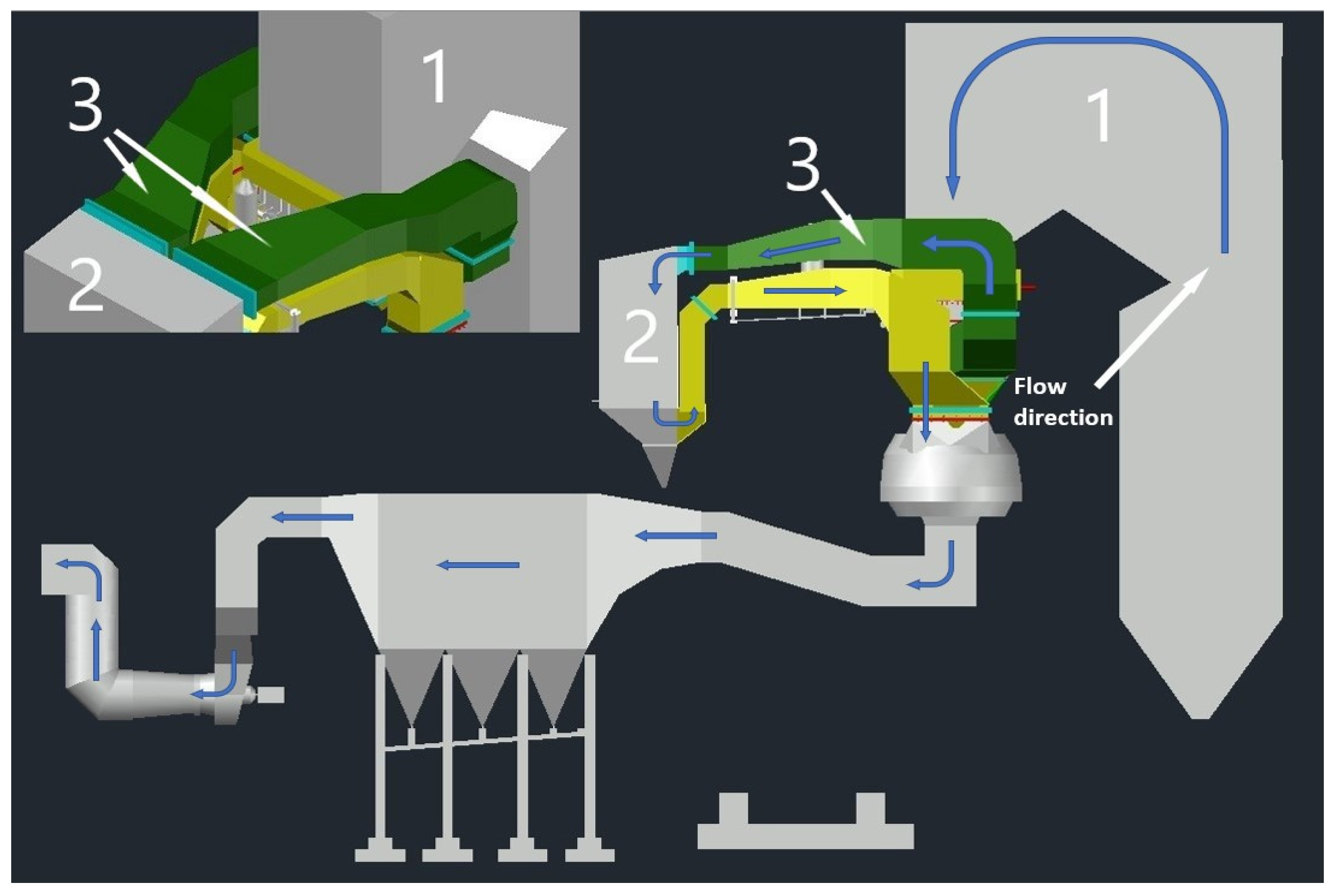
The numerical model includes the flue gas flow through the external duct located downstream of the main boiler flue to the SCR installation, including introducing hot flue gases from the bypass duct into the main flue gas stream. A representative geometry of an OP-650 class coal-fired power boiler was chosen for the study. The analyzed boiler unit schematic with the key components highlighted is shown in
Figure 1: the boiler outline, the SCR installation and the section of pipeline analyzed in this paper placed directly upstream of the SCR installation. In
Figure 1, the flue gas flow path is also marked with blue arrows. The analyzed duct section is symmetrically divided on two sides of the boiler, which is well illustrated by the axonometric view located in the upper left corner of
Figure 1.
For further analyses, a section of the flue gas duct leading from the main boiler building to the SCR installation, marked in
Figure 1 as number 3, was extracted from the presented geometry. As the analyzed duct section upstream of the SCR installation consists of two symmetrical parts, one of them was simulated in the numerical calculations using symmetry conditions.
2.2. The Developed Geometrical Variants
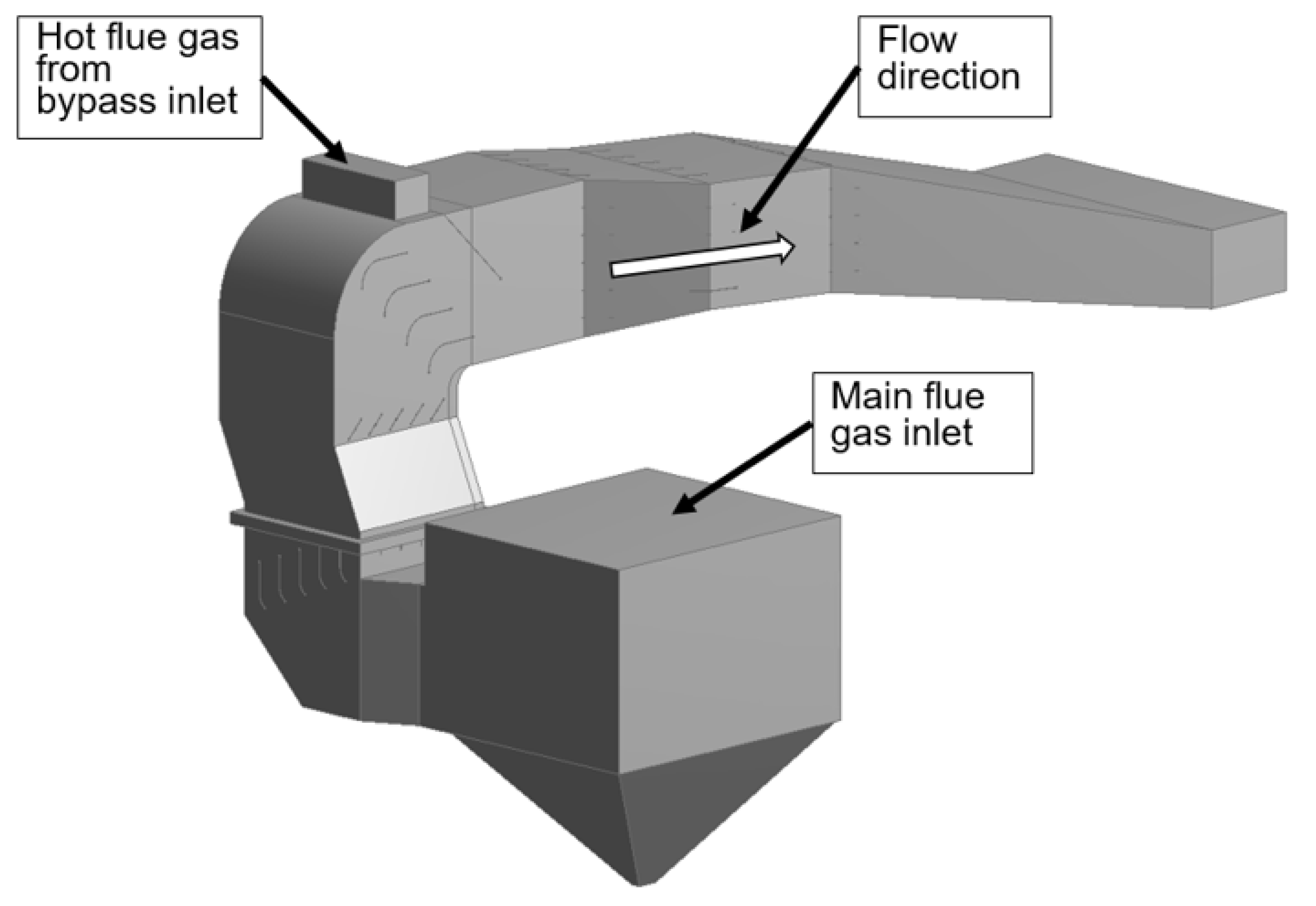
Four selected geometric options are presented in this paper, with the first three reflecting the progress of the fourth and final concept. As mentioned earlier, this study analyzed the bypass duct transporting higher temperature flue gases introduced from the top. The hot flue inlet configuration is the most difficult from the point of view of mixing the flue gas streams before the SCR system. The difficulty in mixing the flue gas streams is mainly due to buoyancy forces and relatively slow flue gas velocities resulting from low boiler load. To obtain a complete representation of the flue gas flow through the analyzed duct section, a full 3D geometry was implemented for the numerical calculations. A general schematic of the examined flue gas duct section is shown in
Figure 2. The section shows the inlets of the flue gas streams and the flow direction towards the SCR reactor.
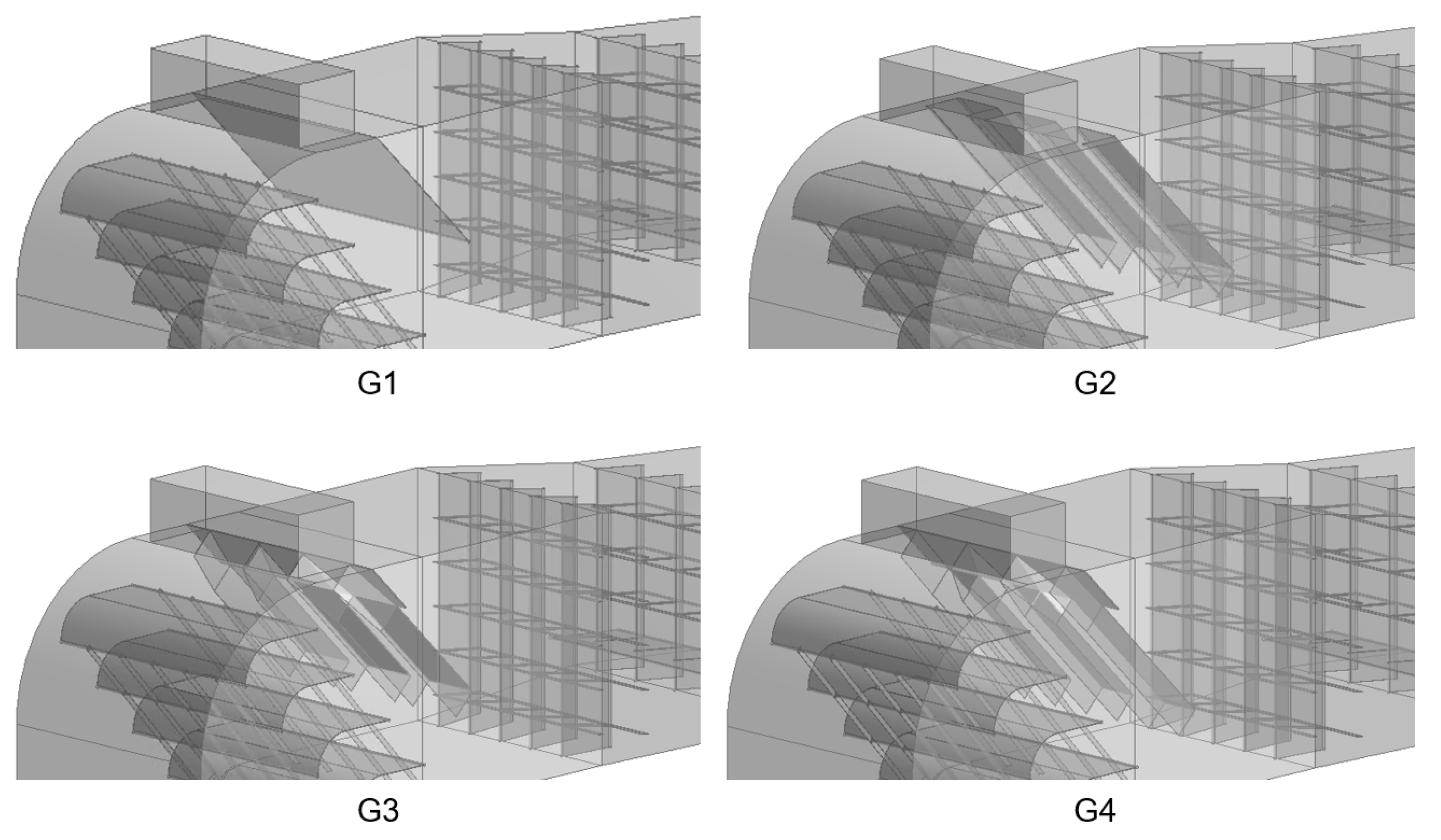
The geometric variants of the turbulence flap are shown in
Figure 3. The geometries presented show the same bypass inlet location in each variant and the evolving geometry of the exhaust gas mixing elements. The other elements in the flue gas duct are fixed vanes which regulate the flue gas flow. The geometric variant G1 involves placing a single flap directly behind the hot flue gas inlet. The flap is inclined at an angle of 45 degrees and its length corresponds to covering half of the duct cross-section. A longer flap could not be used in this solution due to limitations on the maximum flue gas velocity, which increases as the flow cross-section area decreases.
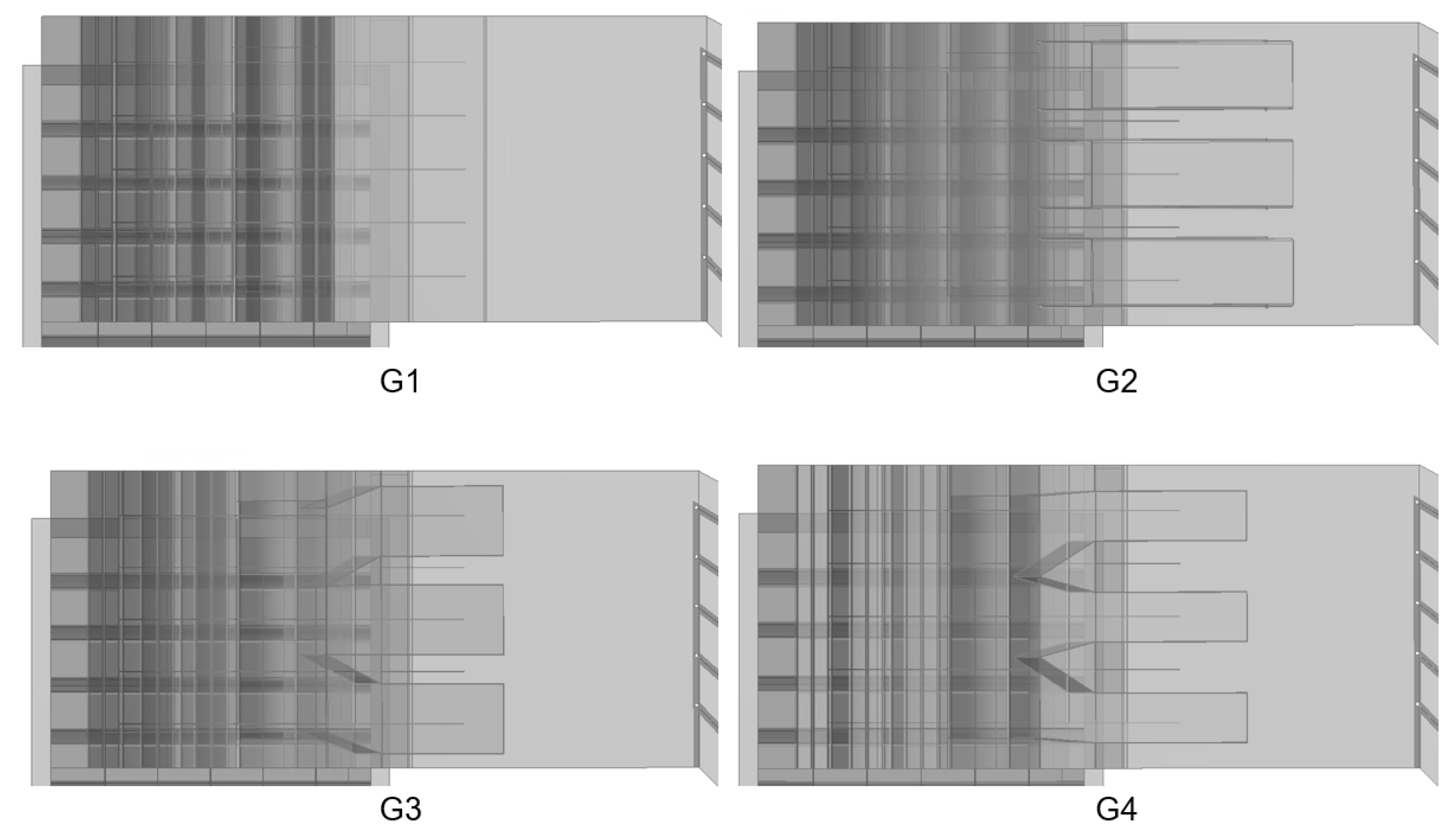
In the geometric variant G2, three U-profiles were placed, with a total width of approximately two-thirds of the channel width and a length corresponding to covering half of the flow cross-section resulting from the velocity condition mentioned earlier. Geometric variations G3 and G4 are a combination of G1 and G2. They use a flat flap in the upper part and three U-profiles in the lower part. Both variants are constructed to cover half of the main duct cross-section. Variant G3 uses shorter but wider U-profiles with a total width of about the main duct of two-thirds. In variant G4, the profiles have a total width corresponding to half the main channel width. The designed geometries of the turbulence flaps, as seen from above, are shown in
Figure 4.
In order to adequately numerically reproduce the effects affecting the exhaust stream mixing, especially the buoyancy forces, the computational geometry was considered at a scale of 1:1. The basic geometrical dimensions of the analyzed channel section are shown in
Table 1.
2.3. Flow-Governing Equations and Model Assumptions
The main equations of fluid mechanics applied to numerical calculations of gas flow such as momentum, mass, energy and species conservation were used for the calculations. They are widely described in many works, e.g., in [
24]. Momentum conservation is represented by Equation (1):
Mass conservation (Equation (2)) is presented below:
Equation (3) represents conservation of energy:
The species conservation is given by Equation (4):
A realizable k-ε turbulence model was implemented for the calculations, with full buoyancy forces included. Detailed descriptions of the above equations and the k-epsilon turbulence model with experimental verification are presented in [
24]. The k-ε realizable model was implemented since it is widely used to calculate free gas flows in relatively large domains, such as in power boilers [
19,
20]. In [
25], this model was used to develop a flow in a large-scale coal-fired boiler. The analyzed channel geometry includes elements that can cause rotation, wall boundary layers and gas recirculation. According to [
26], the applied turbulence model can provide improved numerical simulation results in the abovementioned phenomena. In the k-epsilon model, Reynolds stresses are supplemented by the Boussinesq relation according to Equation (5):
With the turbulent viscosity calculated from Equation (6):
Unlike the standard and RNG models, the value of
is not constant in the k-epsilon realizable model.
is a function of the mean strain and rotation velocities and the turbulence fields represented by k and epsilon. The effective thermal conductivity can be calculated from the following formula (Equation (7)):
Based on the literature [
27], the turbulent Prandtl number was assumed to be 0.85.
In keeping with the character of the flue gas flow passing through the duct in an industrial power boiler, the model adopts the simplifications and basic assumptions outlined below:
Compressible single-phase gas flow;
As there are particulate settlers in the boiler, the existence of fly ash particles is ignored;
Gravity field is included with full buoyancy effects;
The radiation effect is neglected;
Flue gas composition assumed as a result of coal combustion with a relatively high calorific value.
The discrete form of the equations above and all assumptions were implemented in ANSYS Fluent (18.2, ANSYS, Inc., Canonsburg, PA, USA).
2.4. Meshes
As a full-scale 3D channel section simulation was analyzed, considering many elements installed in the channel, such as vanes and a turbulence flap, which require adequate calculation accuracy, so the implemented mesh is relatively large. The work performed a grid sensitivity analysis, examining grids with the following estimated number of elements: 5.5 × 10
6, 11 × 10
6, 17.3 × 10
6, 29 × 10
6, 46 × 10
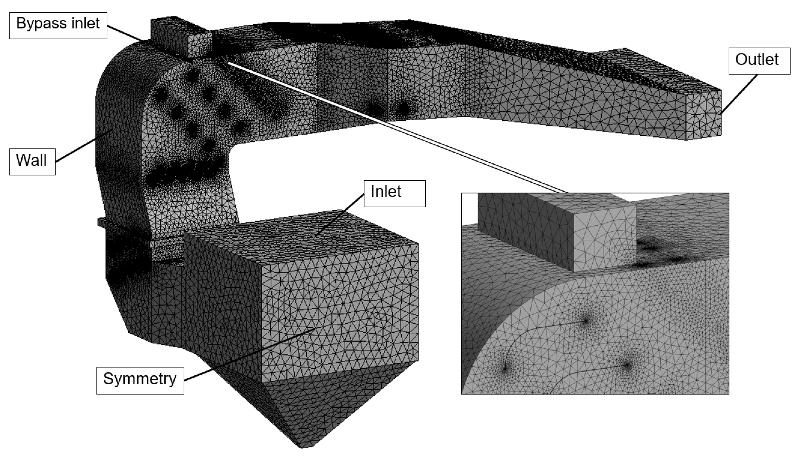
6. The grid element count varies slightly between the analyzed cases, which is a direct result of the different turbulence flap geometries. In investigating the mesh sensitivity, several numerical simulations were performed analyzing parameters such as the final residual sum, mass, energy balance, maximum and minimum temperatures in the domain and pressure drop in the channel. The most reliable results were obtained for grids with 17.3, 29 and 46 million elements. Meshes with approximately 29 million elements were selected for further analysis because the parameters analyzed were highly reliable. The differences between the values obtained in the simulation with the 46 million grid did not exceed 1%. The chosen computational grid is shown in
Figure 5.
As previously mentioned, the analyzed channel section contains many installed irregular-shaped flow control elements that significantly influence the simulation results. Therefore, an unstructured mesh was used in the computational domain, introducing the necessity of using more computing power. The mesh was given appropriately named selections corresponding to the boundary conditions described in the following subsection. The named regions are also shown in
Figure 5.
2.5. Boundary Conditions and Simulations Settings
Each of the computational domains corresponding to the geometric variants was given homogeneous boundary conditions. The zones defined are inlet, bypass inlet, outlet, wall and symmetry, marked in
Figure 5. The inlet boundary condition corresponds to a flow of 90% of the main exhaust stream at a temperature lower than that required for the efficient operation of the SCR reactor. The design inlet type was defined as a mass flow inlet. The main inlet turbulence was specified with the intensity ratio and the hydraulic diameter. Immediately upstream of the design inlet, the boiler has a heat exchanger covering the entire cross-section of the flue gas duct. Therefore, the flue gas flow upstream of the inlet is relatively uniform and regulated, making it possible to apply the uniform velocity field condition at the domain inlet.
The bypass inlet boundary condition corresponds to the higher temperature flue gases introduced into the main duct. These flue gases are led at 10% of the total amount from the higher temperature boiler part. Mixed with 90% of the flue gases from the main duct, they are supposed to ensure the safe operation of the SCR reactor in the appropriate temperature range. The design type of the bypass flue gas inlet is a mass flow inlet type with a uniform perpendicular velocity field. The uniform velocity field simplification was applied due to the relatively large dimensions of the duct, whose cross-section is almost four square meters. The flow is not laminar, and wall effects are negligible. The turbulence was specified with the intensity ratio and the inlet bypass duct hydraulic diameter.
The domain outlet located just upstream of the SCR reactor was defined as a pressure outlet. The appropriate conditions were applied, such as backflow temperature, exhaust composition and turbulence defined by the intensity and hydraulic outlet diameter.
The remaining boundary conditions are the symmetry condition and the wall condition. The symmetry condition was given on one surface, indicated in
Figure 5, and it corresponds to the second, symmetrical part of the boiler, clearly visible in
Figure 1. The wall condition was given on all other surfaces of the computational domain, i.e., the external surfaces of the duct as well as all surfaces corresponding to the flow control elements installed in the duct. All walls both inside and outside the channel were modeled as adiabatic. This approach was justified because the walls inside the duct, which are part of the flow control elements, are heated up to the temperature of the flue gases during the continuous boiler operation. Meanwhile, the external duct walls are well insulated, as indicated by modern temperature measurements installed within the examined boiler section.
The key chemical reactions affecting the flue gas composition no longer occur within the investigated boiler section, so the composition was assumed to be homogeneous for the inlets and the outlet. The flue gas composition and other boundary conditions are shown in
Table 2. As symmetrical duct operation was simulated, the mass values refer to half of the flow.
The key applied solver settings in ANSYS Fluent are coupled scheme with second order discretization for all parameters, pseudo-transient mode, convergence criteria: 10-4. In order to properly evaluate the simulation correctness, relevant parameters were monitored: outlet mass flow, mass-weighted outlet temperature, maximum and minimum temperature in the domain, pressure drop across the duct. The accuracy of the monitored parameters was obtained at a level below 0.1%. Simulations were carried out with a computing server and utilization of 60 cores. The time required to run a single simulation was approximately 8 h.
The numerical model was verified by comparing the current boiler geometry modeling results with the empirical values. The calculations were performed for several operational states of the boiler. The obtained results of temperatures, pressure drops and exhaust gas velocity distribution were compared with the current measurement data. The parameters calculated using the numerical model for the existing boiler structure were convergent with the measured parameters.
3. Results and Discussion
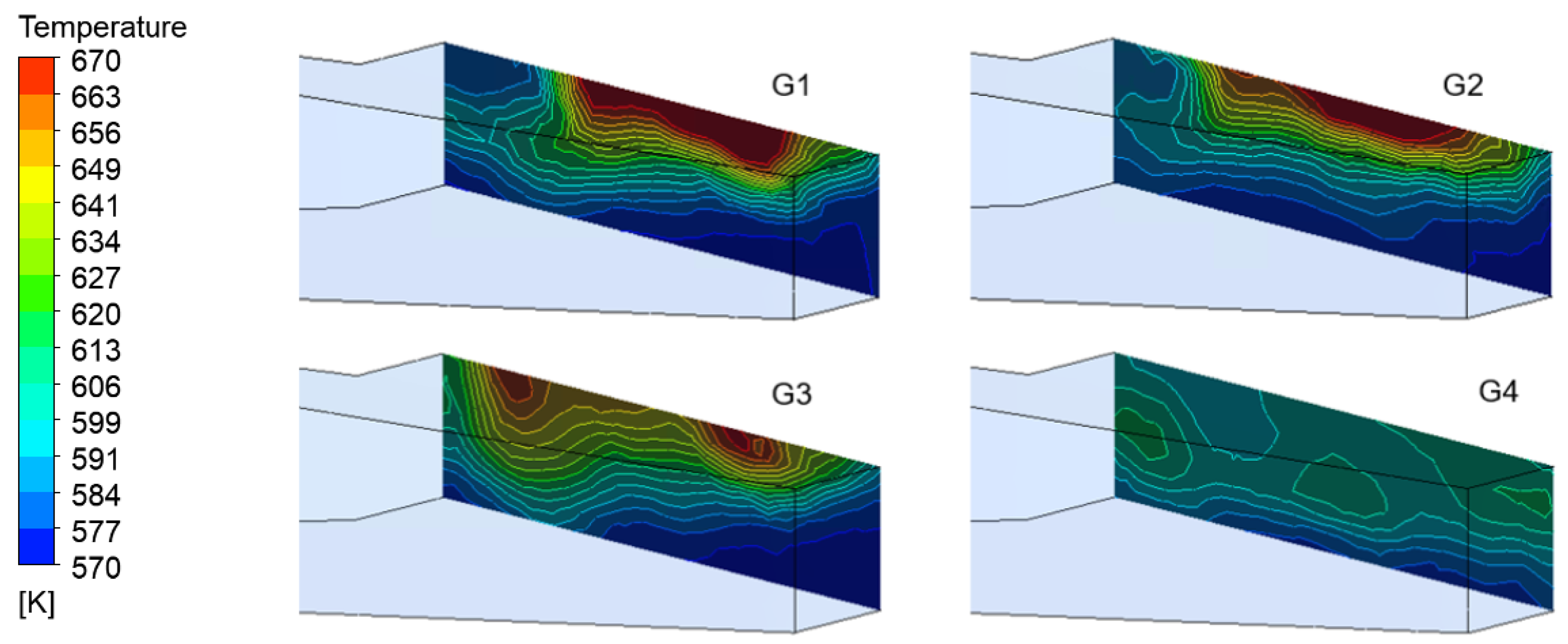
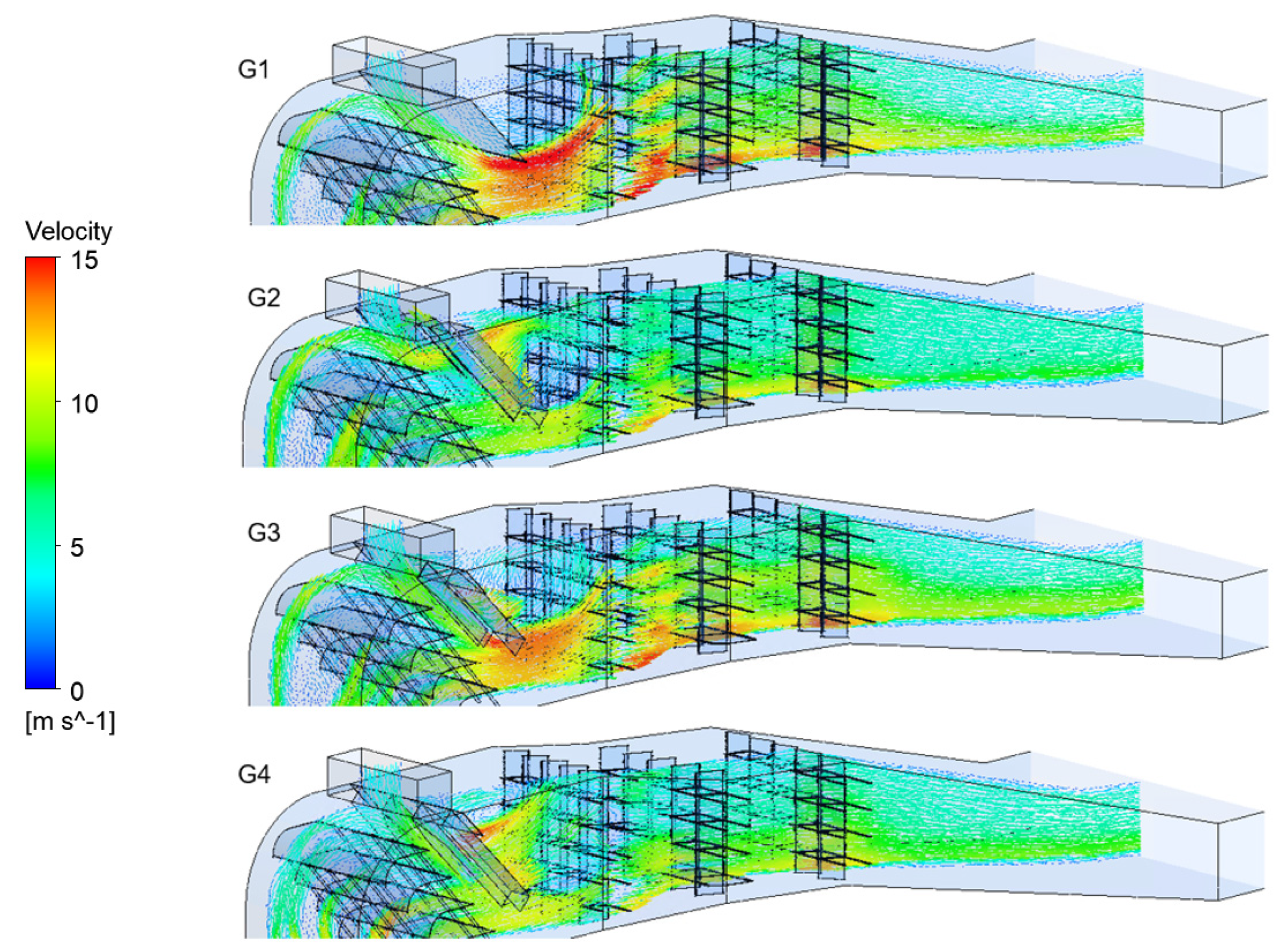
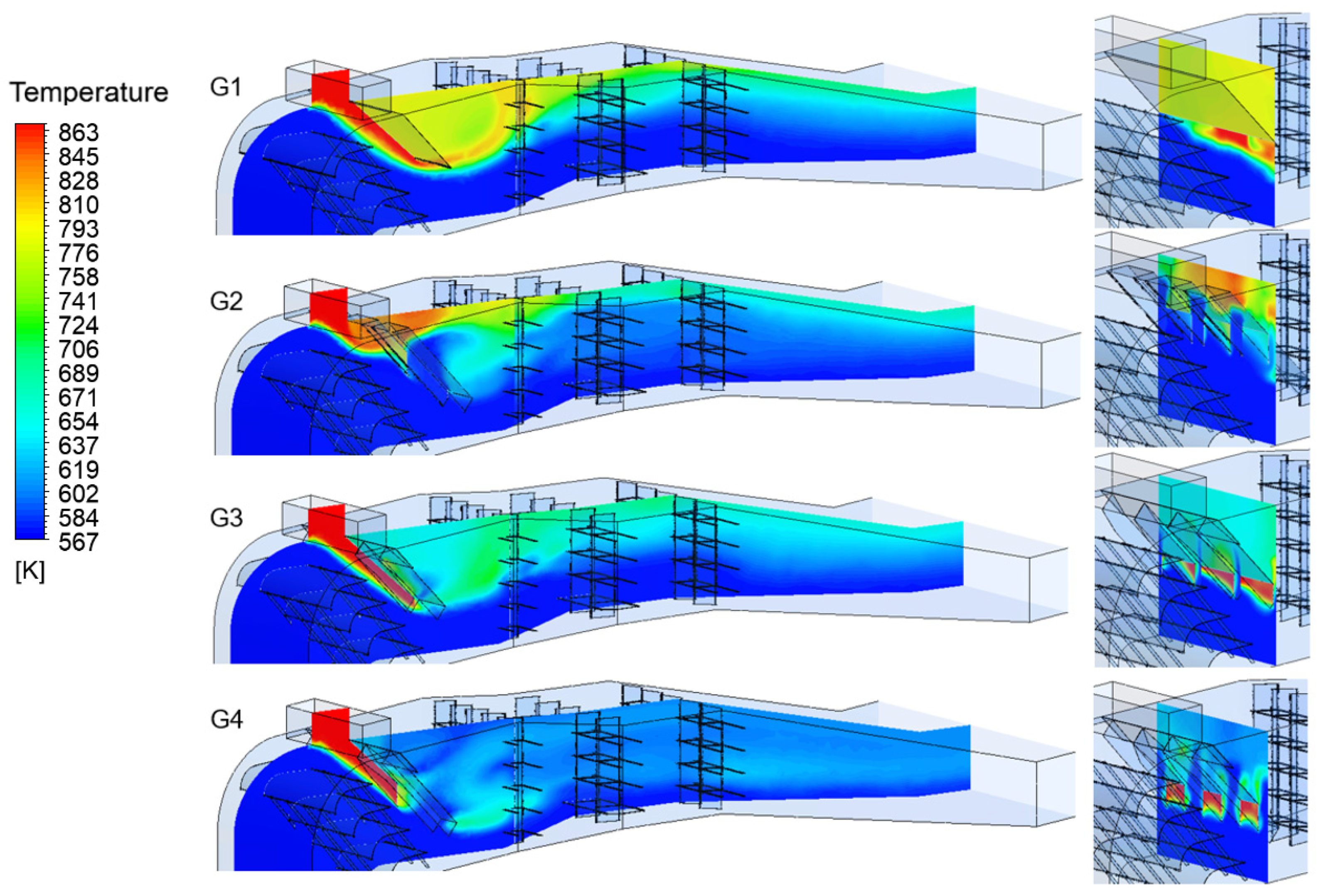
After calculating all geometric variants, and checking the results for correctness through appropriate monitors, the outcomes obtained were evaluated. The most important results testifying the effectiveness of mixing flue gas streams with different temperatures are the temperature fields generated by the calculations carried out. The flue gas temperature distribution for each geometric variant in the plane intersecting the design domain is shown in
Figure 6. The right-hand side of
Figure 6 also shows the temperature distribution on a plane perpendicular to the direction of flow, intersecting the mixing flap.
After analyzing the simulation results, it can be concluded that the most uniform temperature distribution was obtained for the G4 geometric variant. The simulation results of G1 variant indicate that the higher temperature exhaust gas is initially led to the lower part of the duct. However, immediately after the mixing flap, through buoyancy forces and the mass-dominant flow of the denser exhaust gas with a lower temperature, the hot exhaust gas is pushed to the upper part of the duct. They are then mixed to a small extent in the further duct section.
In variant G2, where U-profiles are used, mixing the flue gases is slightly better than in variant G1. In that case, however, most of the hot flue gases right after the bypass duct inlet are forced by the stream of denser and cooler flue gases into the spaces between the U-profiles and flush out the hot flue gases from further parts of the U-profiles. Therefore, the U-profiles installed in this way do not fulfill their intended role, not delivering the hot flue gases to the lower main duct section. Immediately after the mixing flap, the flue gases are directed upwards by buoyancy forces and mix to a small extent in the further section of the duct.
Variant G3 shows an improvement in the level of flue gas mixing compared to variants G1 and G2. The application of U-profiles with a flat section at the flap top allows for an appropriate hot flue gas distribution to the lower parts of the U-profiles. The initial flat section prevents hot flue gases from being washed out by the lower temperature main stream. However, as previously mentioned, the dimensions of each flap had to be adapted to the condition of maximum coverage of half the main duct cross-section. Therefore, U-profiles with a total width of two-thirds the width of the duct cannot be longer. Since the U-profile of variant G3 is wide but relatively short, the hot flue gases are not introduced deep enough to mix effectively with the cold flue gases.
The G4 variant represents the final concept developed, which represents a modification of the G3 variant. Similar to variant G3, a flat section is used in the upper flap section followed by three U-profiles. Variant G4 uses U-profiles that are narrower and longer than the profiles used in variant G3. As with G3, the flat section of the flap prevents the hot flue gases from being washed out in the upper duct section and ensures adequate hot flue gas distribution to the U-profiles. Suitably long profiles transport the hot flue gases to the lower part of the main duct. Then, due to the buoyancy forces, the hot flue gases are mixed with the main flue gas stream of higher density and lower temperature. Further downstream, the flue gas temperature is homogenized. Since the plane on which the temperature is displayed follows the curvature of the flue gas duct, clearly visible in
Figure 1, the hot flue gas portion in the U-profile is cut off, so the observer cannot see the hot flue gas entering the end of the profile.
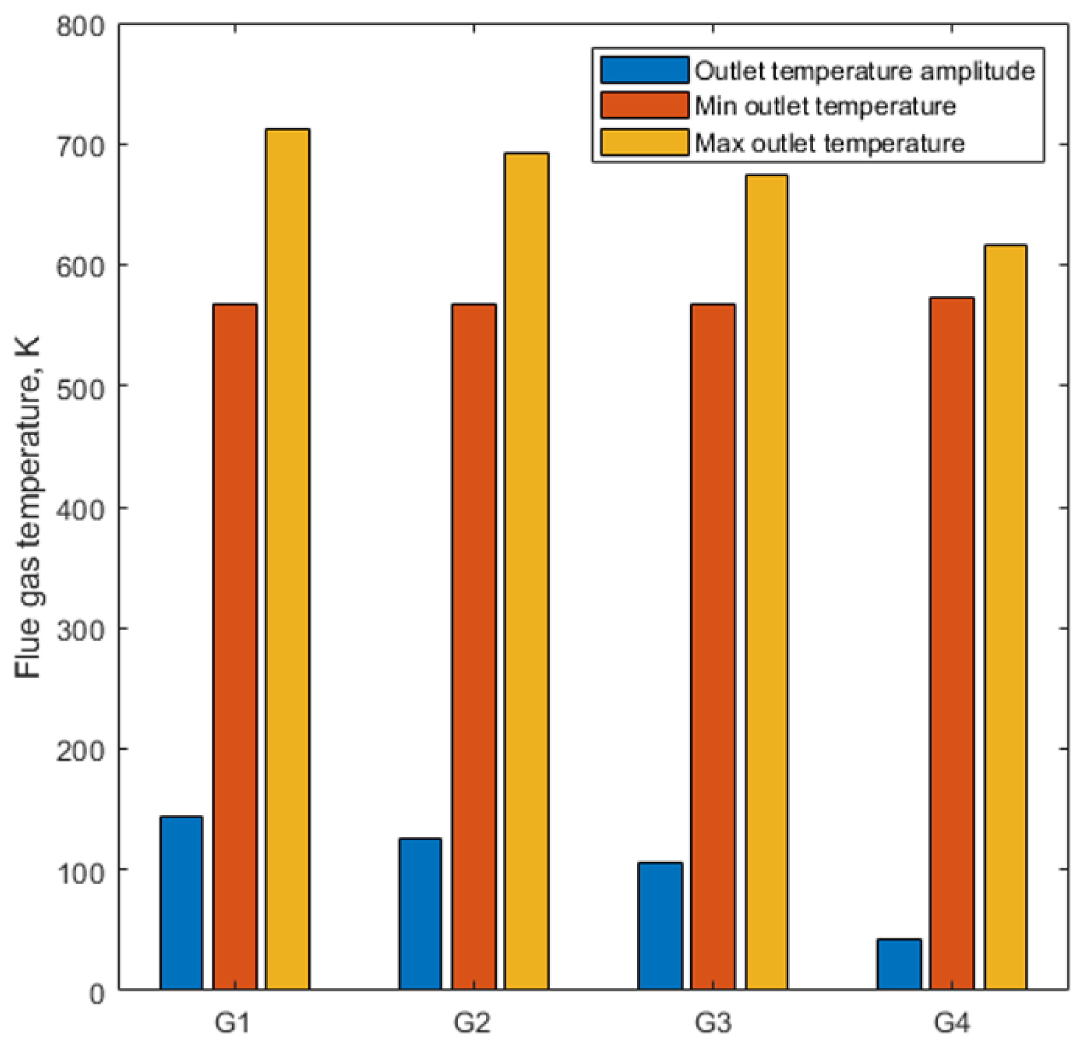
Figure 7 shows the temperature distributions at the computational domain outlet, corresponding to the SCR reactor exhaust inlet. The temperature scale has been narrowed to 100 K (from 570 to 670 K). The target temperature of the perfectly mixed exhaust gas is 597 K. The best degree of mixing of flue gases was obtained in the geometrical variant G4, as can be seen in
Figure 7. In this case, the maximum flue gas temperature was 616 K, which is only 2.18% of the percentage deviation from the perfectly mixed flue gas temperature of 597 K. The minimum flue gas temperature, in this case, was 573.6, which is a deviation of 3.91% from the target temperature. In the cases G1–G3, the temperature amplitudes are considerably larger. All exceed values of 100 K. Simultaneously, in the lower section of the duct, flue gases with a low temperature (close to the initial temperature of the main stream) are observed, which indicates a complete lack of mixing of the lower layers of flue gases.
Figure 8 shows a plot of the minimum and maximum temperatures found for each geometric variant at the outlet of the computational domain representing the inlet to the SCR reactor. The graph also shows the temperature amplitudes at the domain outlet, indicating the degree of exhaust gas stream mixing.
The velocity vectors determined on the plane intersecting the computational domain are shown in
Figure 9. It can be seen that for variant G1, the velocity of the main flue gas stream increases significantly in the area under the turbulizing flap. Meanwhile, a low-pressure field and backflows are created in the upper part behind the flap. In the G2 variant, the flue gases flow freely through the spaces between the turbulence flap’s U-profiles, creating a slight swirl of gas behind the flap. The flow is then stabilized. As in the geometrical variant G1, in the variant G3 with its wide U-profile, the main exhaust flow velocity increases significantly in the area below the flap. Above the flap, a low-pressure field is created together with the backflow. The most uniform velocity field was obtained for variant G4, which is also the most effective in mixing the exhaust gas streams. The main exhaust stream flows gently through the relatively wide spaces between the flap U-profiles. Slight turbulence is created in the upper duct behind the flat part of the turbulence flap.
4. Conclusions
This article presents an innovative method of mixing flue gas streams in a coal boiler using the designed mixing flap. The presented work is concerned with supporting the SCR system operation under low-load conditions of coal-fired boilers, contributing to the flexibility of the operation of these devices. The developed solution was exposed to CFD calculations, in which the distributions of temperature, velocity, density and other key thermodynamic parameters were examined. The results indicate that the invented flap works as intended, causing an adequate mixing of the exhaust gas streams. It results in a uniform gas temperature field before the inlet to the SCR system. The analyses showed that the mixing flap developed by the authors could lower the flue gas amplitude in the desired cross-section from 298 K to 43 K. In the intermediate solutions, amplitudes of 144, 125 and 106 K were obtained. By appropriate mixing, the maximum flue gas temperature was reduced by 251 K. In addition, the developed solution was subjected to computational analyses with regard to its functioning in the case of boiler operation with nominal load. The flap, as previously mentioned, can be folded towards the upper wall of the duct. It allows safe boiler operation in nominal conditions without significant pressure losses in the flue gas duct.
The developed solution entails investment costs and operating costs. However, due to the current energy policy and the need for coexistence of coal-fired boilers with renewable energy sources, such solutions are necessary for these facilities to function. As in the flue gas treatment installation, this type of modernization does not provide direct profits from the implementation but allows the facility to operate in new conditions of the energy system.
It is planned to create a construction design and then install the device on the OP-650 boiler in the longer term. Work will then be carried out to optimize the method. The next steps will involve the application of the method in coal boilers with different power ranges. Although the solution is dedicated to power boilers, it is possible to use the developed concept in other systems requiring mixing gases with different temperatures.


