


Abstract
Korean firms record the cost of entertaining customers and counterparties in a separate account and report it on its own where they judge it material. The COVID-19 pandemic interrupted the activity that account pays for. This study asks whether the stock market’s valuation of that spending changed around the interruption. Using 19,334 firm-years on 2331 Korean listed firms from 2016 to 2025, Tobin’s Q is regressed on reported entertainment expenditure scaled by sales and interacted with indicators for the pandemic years 2020 to 2021 and the years that followed, with firm and year fixed effects and standard errors clustered by firm. Entertainment intensity was positively associated with firm value before the pandemic, although that association is carried by the heaviest spenders and does not survive their removal. The pandemic interaction is imprecise, running from −20.81 to 11.66 against a benchmark of 21.916. After the pandemic, the association was eliminated: the interaction is −29.655, and it holds across nine measurement and deflator variants. The association changes sign around 2022; a test that does not impose the date locates the change there, but a discrete break and a decline that steepens cannot be separated. Advertising and research intensity attenuate at least as much, so the change belongs to discretionary expenditure as a class rather than to entertainment alone.
Keywords:
business promotion expense; entertainment expenditure; value relevance; Tobin’s Q; COVID-19; Korean stock market; voluntary disclosure; panel fixed effects JEL Classification:
G32; M41; M21; G14
1. Introduction
Korean firms report what they spend entertaining customers, suppliers and officials on a line of its own, within selling and administrative expense in the income statement and, for manufacturers, within the manufacturing cost statement. Separate reporting is permitted rather than required, and about four firm-years in five carry it. The account is called business promotion expense, and until recently, it was an unremarkable part of doing business in Korea. Firms spent on it, auditors signed off on it, and the tax code capped how much of it could be deducted. Then, for two years, the account was hard to use. Korea ran a tiered social distancing regime from May 2020 to April 2022, under which the trading hours of restaurants were restricted, some venues were closed outright, and private gatherings were capped at four people at the tighter levels (Bahk et al., 2023). The activity the account pays for was curtailed for long stretches in 2020 and 2021.
That interruption is the setting of this paper. The question is not whether firms spent less, which they plainly did, but whether the stock market changed its mind about what the spending is worth. Entertainment spending is one of the few outlays that is simultaneously an investment in relationships and a candidate for waste, and which of the two readings dominates is an empirical matter that could plausibly shift when the underlying activity is disrupted. The literature on managerial perquisites reads spending of this kind as consumption that shareholders would rather not fund (Rajan & Wulf, 2006; Yermack, 2006), while the literature on discretionary intangible outlays reads expensed spending as investment the market capitalises anyway (Erickson & Jacobson, 1992; Lev & Sougiannis, 1996). If relational capital is what the account buys, a crisis that threatens continuity should make it more valuable, not less. If the account is closer to perquisite consumption, a forced pause gives the market a natural experiment in doing without it.
Two features of the Korean setting make the question answerable here in a way it is not in most markets. The first is that the item can be seen at all. In the United States, entertainment costs sit inside selling, general and administrative expenses and cannot be separated from it. Korean firms report the item on a line of its own, in the income statement and, for manufacturers, in the manufacturing cost statement, and about four firm-years in five carry it. A firm-year measure can therefore be built from the financial statements themselves for the great majority of the market. Separate reporting is a presentation choice rather than a requirement, and that is a limitation this paper takes seriously and returns to in Section 6.3. The second feature is that the disruption was to the activity and not merely to its reporting. Accounts that change because a standard changed tell us about accounting, and much of what the value relevance literature has documented about weakening associations turns on changes of that kind (Collins et al., 1997; Francis & Schipper, 1999). This account changed because people stopped meeting.
The study covers 2016 through 2025 and splits the decade into the four years before the pandemic, the two years of it, and the four years after. That last window is what distinguishes this paper from work written while the pandemic was still running. Studies completed in 2021 or 2022 could observe the shock but not its aftermath, and the aftermath turns out to be where the interesting variation lies.
The gap this fills is one of timing rather than of subject. Work on corporate outcomes during COVID-19 was necessarily written while the episode was running, and it establishes which firms proved resilient and why (Ding et al., 2021; Fahlenbrach et al., 2021; Ramelli & Wagner, 2020; Albuquerque et al., 2020). What such work cannot observe is whether anything it documented persisted. Evidence on discretionary intangible spending in Korea over an overlapping window reports the same shape for advertising, an association that strengthens during the pandemic and weakens afterwards (Kwon, 2025); that study is the present author’s own, which covers fiscal 2018 to 2023, and it stops two years before the window observed here closes. Four post-pandemic years are now observable, and the question of whether a shock changed a durable practice or merely interrupted it can be asked of the data rather than assumed. That is what makes the question worth answering now and not in 2022: an interruption and a permanent change look identical while the interruption is still running, and they can only be told apart afterwards. The distinction matters beyond this account. Firms and investors are still deciding which of the working practices that the pandemic suspended are worth restoring, and a market that stopped paying for one of them is evidence about that decision.
The results are not the ones the relational-capital view predicts. Through 2021, the market paid for entertainment spending: firms that spent more, relative to sales, carried higher valuations. The pandemic interaction is small and imprecisely estimated, with a ninety-five per cent interval running from −20.81 to 11.66 against a pre-pandemic benchmark of 21.916, so the hypothesis that the crisis raised the value of the account is rejected, while exact equality is not established. It is after the pandemic that the relation breaks. From 2022, the year-by-year coefficients turn negative and the pooled post-pandemic association can no longer be distinguished from zero. That change is the robust result in this paper: it holds across nine measurement and deflator variants, with a post-period interaction between −23.629 and −38.330, and the association changes sign around 2022, although the shape of the change is not identified. The pre-pandemic association itself is more fragile and rests on the upper tail of the spending distribution.
Capital markets research has long asked what accounting amounts tell investors and under what conditions the answer changes (Kothari, 2001). The theoretical contribution of this paper is to put two competing readings of relational spending against a natural interruption of the activity itself and to find that neither survives intact. The relational view predicts that a threat to continuity raises the value of investments in relationships; the pandemic interaction gives no support for that. The agency view predicts that spending of this kind destroys value; the pre-pandemic association is positive, though it depends on heavy spenders. What the evidence supports is narrower and less comfortable than either: the account was priced before 2022 and is not priced after, and the same is true for advertising and for research spending, so the change belongs to discretionary expenditure as a class rather than to entertainment as an activity. A second theoretical contribution is methodological in the value relevance tradition. Where an association is reported to have weakened, the weakening is usually attributed to the item; this paper shows what a same-design comparison against other discretionary items does to such an attribution.
The practical contribution is twofold. For managers and boards, entertainment budgets restored to their pre-2020 scale are not being read by investors as they were before 2020, and the evidence here says the same for advertising and research intensity. For preparers and for those who set disclosure requirements, the paper documents that a firm’s decision to show this account separately is unrelated to its valuation, that the largest firms are the least likely to show it, and that the proportion showing it has fallen in every year of the sample. An item that is material to the question an outside user wants to ask is left to a presentation judgement, and it is the firms with the largest absolute spending whose amounts are least often visible.
The paper proceeds as follows. Section 2 describes the institutional setting and the literature the study draws on. Section 3 develops the hypotheses. Section 4 sets out the research design and the sample. Section 5 reports the main results and Section 6 the additional analyses. Section 7 discusses the findings and their implications, and Section 8 concludes.
2. Institutional Background and Related Literature
2.1. Business Promotion Expense in Korea
Business promotion expense is the account in which Korean firms record the cost of entertaining customers, suppliers and counterparties. Neither the Korean accounting standards nor the international standards Korea adopted require it to be shown on a line of its own (Y. K. Lee, 2021). Separate presentation is permitted rather than required: a firm is free to show the item within selling and administrative expense or to fold it into that aggregate, and where expenses are classified by function, the detail appears in the notes rather than on the face of the statement. Separate presentation is therefore a reporting choice, most plausibly a judgement about materiality relative to the firm’s own cost base, and it has been shown to vary with governance (Y. K. Lee, 2021). In the sample used here, it is made in 77.9 per cent of firm-years. It is made least often at the largest firms, which are the firms least likely to have spent nothing: the share reporting the item separately is above eighty-three per cent in the smallest size quintile in every period and between 58.6 and 60.5 per cent in the largest. Section 6.3 returns to this. What follows, and every estimate in this paper, concerns entertainment expenditure as reported.
Manufacturers report the item twice where they present both statements, because costs attached to production flow through the manufacturing cost statement, while costs of selling and administration appear in the income statement. The manufacturing cost statement has not been a required disclosure item since the mid-2000s, and the proportion of manufacturers in this sample presenting any of its detail falls from 36.4 per cent in 2019 to 12.5 per cent in 2025. The measure used here adds the manufacturing figure where it is available, and the robustness tests in Section 5.4 report the estimate built on the income statement alone.
The tax treatment gives the account further significance. Korean tax law caps the deductible amount at a fixed annual allowance plus a proportion of revenue, and expenditure beyond the cap is not deductible; the cap is set by Article 25 of the Corporate Income Tax Act and its enforcement decree. Three changes fall within the sample window. From fiscal 2020, the fixed allowance for small and medium enterprises rose from 24 to 36 million won and the revenue-proportional rate rose from 0.2 to 0.3 per cent on revenue up to 10 billion won and from 0.1 to 0.2 per cent on that between 10 and 50 billion. From fiscal 2021, the threshold above which qualified documentary evidence is required rose from 10,000 to 30,000 won per occasion. From fiscal 2024, the statutory term for the account was changed, with its substantive scope unchanged. None of these falls at or near 2022, which is where the change documented in Section 5 is located. The 2020 relaxation runs against that change rather than towards it: it made the account cheaper at the margin in the first pandemic year.
One further piece of the regulatory setting matters for how the pre-pandemic years should be read. The Improper Solicitation and Graft Act took effect on 28 September 2016, in the first year of the sample. It caps what a public official, or an employee of a media company or private school, is permitted to accept from one person at one million won on a single occasion and three million won in a fiscal year, and it exempts meals below 30,000 won and gifts below 50,000 won offered in the course of a social relationship. Its constraint falls directly on the activity this account pays for. Aggregate entertainment expenditure reported to the National Tax Service fell from 2.95 trillion won in 2016 to 2.63 trillion in 2019 on that authority’s own published figures, and evidence from public procurement auctions indicates that the bidding advantage associated with entertaining officials narrowed after the statute came into force (Kang et al., 2023). The pre-pandemic window against which the pandemic and post-pandemic slopes are measured is thus not a period of settled practice. It is a period in which entertainment spending was already under regulatory pressure, and the estimates in Section 5 should be read with that in view.
Spending in this account is visible where it is separately reported, capped for tax purposes, and constrained by statute in one of its uses. That combination is unusual for a discretionary cost and is what makes the question in this paper answerable.
2.2. What the Account Might Represent
Two readings of entertainment spending compete in the literature, and they carry opposite predictions. The first is the relational view of competitive advantage, which treats the account as an investment in relationships that generate rents outside the boundaries of the firm. The second is agency theory, which treats it as discretionary spending that managers control but do not fund themselves, and therefore as a channel for private benefit. Both are tested here within the value relevance tradition that follows from the residual income model, in which an accounting amount is value-relevant if it is associated with market value conditional on the other information investors hold (Ohlson, 1995; Feltham & Ohlson, 1995).
Under the first, the account buys relational capital. The relational view of competitive advantage holds that returns can accrue to relationships between firms rather than to assets held within them, and that investments in relationship-specific routines and trust are a source of rents that arm’s-length transacting cannot replicate (Dyer & Singh, 1998). Entertainment spending is a plausible instrument of such investment in economies where business is conducted through personal ties, and the East Asian literature on guanxi describes exactly that: personal connections substituting for weak formal institutions, cultivated deliberately and at cost (Xin & Pearce, 1996; Park & Luo, 2001). On this reading, the account is an intangible investment, and the market should price it as one.
Under the second, the account is a channel for private benefit. Where managers control resources they do not own, spending that is difficult to monitor and pleasant to consume is a classic vehicle for the diversion of firm value (Jensen & Meckling, 1976). Entertainment has precisely those properties, and the evidence on perquisites bears the reading out: corporate jets and similar benefits are associated with lower shareholder returns (Yermack, 2006), although perquisites can also be efficient where they substitute for cash compensation or improve productivity (Rajan & Wulf, 2006). In China, where the institutional setting resembles Korea’s in the salience of relationships, executive perks have been linked both to firm performance and to less informative stock prices (Adithipyangkul et al., 2011; Gul et al., 2011). The evidence from China is instructive here: entertainment and travel costs are associated with the payment of bribes and with managerial excess as well as with the building of relationships, so the same account carries both meanings within a single economy (Cai et al., 2011). Relatedly, where relationships with government or lenders are valuable, firms that cultivate them obtain favourable treatment, which is a reason for the market to price connection-building positively even where the mechanism is unattractive (Khwaja & Mian, 2005). Political connections carry measurable value in a wide cross-section of countries (Faccio, 2006), and in China, connected private firms obtain financing and perform better than unconnected ones (Li et al., 2008).
The two readings are not mutually exclusive, and which dominates in a given firm-year is what the valuation evidence reveals.
2.3. Valuing Discretionary Intangible Spending
The value relevance literature asks whether accounting amounts are associated with market values in the way a valuation model implies, taking the residual income framework as the organising structure (Ohlson, 1995; Feltham & Ohlson, 1995). That literature has been criticised for what it can and cannot tell standard setters, and the criticism is worth keeping in view: an association between an accounting number and price is evidence about pricing, not about the usefulness of a standard (Barth et al., 2001a; Kothari, 2001). The present paper makes the narrower claim. It also sidesteps the question of earnings quality, on which the choice of proxy matters a great deal (Dechow et al., 2010), by taking a single disclosed expenditure rather than a constructed measure of reporting quality.
Work on discretionary intangible outlays has established that the market capitalises spending that accounting expenses. Research and development expenditure is priced as an asset rather than as a cost (Sougiannis, 1994; Lev & Sougiannis, 1996), and advertising and research spending both carry valuation consequences that survive controls for profitability and size (Erickson & Jacobson, 1992; Chauvin & Hirschey, 1993). The marketing literature reaches the same conclusion from the other direction, finding that advertising affects firm value through both direct and indirect channels (Srinivasan & Hanssens, 2009; Joshi & Hanssens, 2010). Non-financial measures of activity can be value-relevant where recognised assets capture little of what a firm has built (Amir & Lev, 1996), and intangible intensity shapes how much information reaches the market in the first place (Barth et al., 2001b). The association is not stable over time. Earnings have lost explanatory power relative to book values across four decades of US data (Collins et al., 1997), and whether that amounts to a loss of relevance depends on how the question is posed (Francis & Schipper, 1999). The relation between accounting numbers and market values weakened as intangible investment grew relative to recognised assets (Lev & Zarowin, 1999), and the apparent shifts in how the market valued particular items during the technology boom proved on examination to be less novel than they appeared (Core et al., 2003). That last finding is a caution this paper takes seriously: a coefficient that moves across periods needs to be shown to move at a particular time, not merely to differ between arbitrary windows. The question this paper asks has been put to a neighbouring account over an overlapping window: advertising intensity in the same market is positively associated with firm value, more strongly during the pandemic and less strongly afterwards (Kwon, 2025). That study ends in 2023 and does not cover entertainment expenditure, and the present paper extends both the window and the account.
2.4. The Pandemic as a Setting
Research on corporate outcomes during COVID-19 has concentrated on which firm characteristics conferred resilience. Financial and organisational strength, supply-chain position and ownership structure all shaped how firms’ equity fared through the shock (Ding et al., 2021), and financial flexibility mattered a great deal when revenue stopped (Fahlenbrach et al., 2021). Prices moved in response to exposure to the virus within weeks of the outbreak (Ramelli & Wagner, 2020), and stocks rated highly on environmental and social criteria proved more resilient through the crash (Albuquerque et al., 2020), which suggests that investors did reprice non-financial firm attributes under stress. Much of this work necessarily ends in 2020 or 2021.
What the later window adds is the possibility of distinguishing a shock from a change. Evidence on remote work suggests that the pandemic shifted practice permanently rather than temporarily, with a large fraction of the shift to working from home expected to persist after the health emergency passed (Barrero et al., 2021). That expectation rests on more than the pandemic episode. A randomised experiment before COVID-19 had already shown remote work to be productive rather than merely tolerable (Bloom et al., 2015), and geographic flexibility raised output when a US agency adopted it (Choudhury et al., 2021). If face-to-face business entertainment underwent a similar adjustment, the observable consequence would appear after 2021 rather than during the pandemic and would not reverse. Korean evidence puts the size of the shock to corporate spending in view: outside the business groups, firms cut investment to about two-fifths of its pre-crisis level in the first quarter of 2020, while group-affiliated firms barely adjusted (S. Lee, 2022).
3. Hypotheses
Each hypothesis below is a prediction on which the two theories set out in Section 2.2 differ, and the sign of the estimate is what discriminates between them.
H1.
Business promotion expenditure is positively associated with firm value over the sample period as a whole.
This is the baseline the rest of the design is measured against. The relational reading predicts a positive association, since spending that builds durable customer and supplier relationships should support future cash flows that the accounting system expenses immediately. Prior evidence that the market capitalises other expensed intangible outlays supports the prediction: research spending is priced as an asset (Sougiannis, 1994; Lev & Sougiannis, 1996), advertising and research both yield measurable valuation returns (Erickson & Jacobson, 1992; Chauvin & Hirschey, 1993), and non-financial indicators of activity are priced where recognised assets are silent (Amir & Lev, 1996). If entertainment spending accumulates relational capital in the sense of Dyer and Singh (1998), it belongs in that group.
The agency reading predicts the opposite. Perquisite consumption destroys value where it is not disciplined (Yermack, 2006), and entertainment is harder to monitor than most line items. The hypothesis is therefore posed with a directional prediction but a live alternative, and the sign is what discriminates between the two readings. A null would indicate that they roughly offset in the average firm-year, which is itself worth establishing before any period comparison is attempted.
H2.
The association between business promotion expenditure and firm value is stronger during the COVID-19 period than before it.
A crisis raises the value of evidence that a firm will still be there when it ends. Where financial disclosures deteriorate simultaneously for everyone, non-financial indications of commitment to counterparties carry more information than usual, and relational capital is most valuable precisely when contracts are hardest to enforce and continuity is least certain (Dyer & Singh, 1998). The guanxi literature makes the same point about institutional weakness: connections matter most where formal support is least reliable (Xin & Pearce, 1996), and connected firms obtained financing when unconnected ones could not (Li et al., 2008). There is direct evidence that investors repriced non-financial attributes during this particular crisis, favouring firms with stronger environmental and social profiles (Albuquerque et al., 2020) and reacting within weeks to differences in exposure (Ramelli & Wagner, 2020). Firms that sustained spending on relationships while their peers cut it were making a costly and observable choice. If the market reads the account as relational investment, that choice should have been rewarded.
Rejection would be informative in its own right. It would mean either that the market does not read the account as a commitment signal, or that whatever signalling value the spending carries is swamped during a crisis by concerns about cash preservation, which mattered more than most firm attributes in 2020 (Fahlenbrach et al., 2021).
H3.
The association between business promotion expenditure and firm value is weaker after the COVID-19 period than before it.
Two mechanisms point the same way, which matters for how a null should be read. The first is substitution: two years of conducting business remotely demonstrated that a substantial part of what entertainment spending accomplished could be accomplished without it, and the evidence on remote work suggests such demonstrations do not reverse when the constraint is lifted (Bloom et al., 2015; Barrero et al., 2021; Choudhury et al., 2021). The second is monitoring: an episode in which firms discovered they could operate on reduced entertainment budgets makes subsequent heavy spending harder to defend as necessary, which shifts the balance between the relational and agency readings towards the latter (Jensen & Meckling, 1976). Where perquisite-type spending is read as excess rather than investment, it is associated with lower valuations and with prices that impound less firm-specific information (Yermack, 2006; Gul et al., 2011).
Because both mechanisms predict weakening, the hypothesis is directional. What neither predicts is a change of sign, and the distinction between attenuation and reversal is therefore diagnostic. Figure 1 sets out the design as a whole: the question, the setting, the three hypotheses with the theory behind each, the variables and the identification strategy.
Figure 1.
Research design: question, hypotheses, variables and identification. TOBINQ is Tobin’s Q and BPE is business promotion expenditure scaled by sales. The controls are advertising intensity (AD), research and development intensity (RD), firm size (SIZE), leverage (LEV), return on assets (ROA), sales growth (GRW), intangible intensity (INT), property, plant and equipment intensity (PPE), operating cash flow (CFO) and firm age (AGE). Each variable is defined in full in Section 4.3.
4. Research Design
4.1. Model
The tests estimate
where TOBINQ is Tobin’s Q, BPE is business promotion expenditure scaled by sales, COVID indicates the fiscal years 2020 and 2021 and POST indicates 2022 through 2025; Section 4.3 defines each variable in full. The period main effects are absorbed by the year fixed effects and are not separately estimated.
TOBINQi,t = b0 + b1 BPEi,t + b2 BPEi,t × COVIDt + b3 BPEi,t × POSTt + Controlsi,t + firmi + yeart + ei,t
The specification is an interacted value relevance regression rather than a residual income model estimated directly. The choice follows the applied convention in this literature, which regresses a market-based measure on the accounting item of interest and a set of fundamentals rather than imposing the full structure of the valuation identity (Ohlson, 1995; Feltham & Ohlson, 1995; Barth et al., 2001b). Nothing in the hypotheses requires the stronger structure, and imposing it would restrict the controls in ways that are hard to defend when the item under study is a single expensed outlay.
The coefficient b1 is the association between entertainment intensity and value in the pre-pandemic years and tests H1. The interactions b2 and b3 are differences relative to that benchmark and test H2 and H3, so that the association during the pandemic is b1 + b2 and the association after it is b1 + b3. Reporting these sums separately matters because a negative b3 is consistent both with a return to indifference and with active discounting, and only the sum distinguishes them; the two are reported as linear combinations of the estimated coefficients.
A simpler design would split the sample into three periods and compare coefficients across subsamples. That is avoided here for two reasons. Subsample estimation discards the cross-period restriction on the control coefficients, so any difference in the entertainment slope is confounded with differences in how the controls operate, and it provides no direct test of whether the slopes differ, which the interaction terms supply. Where a design compares outcomes across periods, inference also has to contend with serial correlation within units, and comparing point estimates from separate regressions makes that harder rather than easier (Bertrand et al., 2004).
Firm fixed effects absorb the possibility that firms which entertain heavily differ persistently from those which do not in ways that also affect valuation, which is the first-order concern in a cross-section of this kind: industry, business model, customer concentration and managerial style are all plausible common causes and all are largely time-invariant over a decade. Identification therefore comes from changes within a firm over time. The alternative of controlling for the unobserved heterogeneity by including group averages or by adjusting the dependent variable is known to be biased, and the fixed effects estimator is the appropriate instrument where the heterogeneity is at the unit level (Gormley & Matsa, 2014).
In the estimation, the firm effects are absorbed by the within-firm transformation and the year effects enter as dummy variables, with 2025 as the base year. The year dummies are demeaned along with every other regressor, so that the coefficients are numerically identical to those from an estimation that includes 2331 firm dummies and nine year dummies directly. The coefficients from this transformation were confirmed against a full least-squares dummy variable estimation before the results were taken as final, and agree to nine decimal places; in an unbalanced panel, that equivalence does not hold if the year dummies are left untransformed.
Standard errors are clustered by firm. A firm’s residuals are correlated across the ten years it appears, and treating firm-years as independent overstates precision substantially in panels of this shape (Petersen, 2009). Clustering on the firm dimension addresses that correlation and, because the year effects are removed by dummies, the residual cross-sectional dependence that would motivate a second clustering dimension is largely absorbed (Cameron et al., 2011). Degrees of freedom are set by the number of clusters rather than the number of observations, which is the conservative choice with 2331 firms. Standard errors are computed from the survey-design variance estimator of PROC SURVEYREG in SAS 9.4, with one adjustment. Because the firm effects are removed by the within transformation rather than entered as regressors, that procedure does not account for them when it forms its finite-sample correction, and the standard errors it reports are accordingly too small. They are multiplied by the square root of (N − k)/(N − k − (G − 1)), where N is the number of firm-years, k the number of regressors in the transformed model and G the number of firms. In the main specification, N is 19,334, k is 23 and G is 2331, so the factor is 1.0664, and the total degrees of freedom the correction restores, 23 + 2330 = 2353, is the number PROC PANEL reports for the same model estimated with two-way fixed effects. All standard errors, t-statistics and p-values reported in the paper incorporate the adjustment. The correction is the usual finite-sample cluster adjustment for a linear model with clustered errors, applied to an estimator whose absorbed effects the procedure does not account for (Cameron & Miller, 2015; Correia, 2017). The adjustment was verified in three ways. The model was estimated in dummy-variable form on subsamples small enough for that to be feasible, where the coefficients agree to nine decimal places and the ratio of the two standard errors matches the factor above to five decimal places. The reported degrees of freedom were checked against PROC PANEL with two-way fixed effects, which gives 16,981, so that N minus the residual degrees of freedom is exactly 2353. And the main specification was re-estimated in an independent implementation written for this revision, which absorbs the firm effects and forms the clustered variance directly with the correction that the reghdfe package applies, namely (G/(G − 1)) × ((N − 1)/(N − K)), with K counting the absorbed effects; that implementation reproduces the coefficients to eight decimal places and the standard errors as printed, at 6.797, 8.277 and 8.276. The two routes differ in the fourth decimal place of the scaling factor, 1.0664 against 1.0672, and agree on every standard error the paper reports.
A remark on one control that is deliberately absent. The book-to-market ratio is a standard control in valuation regressions, but its denominator is the market value of equity, which is also the numerator of Tobin’s Q. Including it induces a mechanical negative association that inflates explanatory power without reflecting anything economic; in this sample, it carried a t-statistic of −24.9 and roughly doubled the reported R-squared while leaving the coefficients of interest essentially unchanged. It is excluded. Replacing it with the book value of equity scaled by assets is not an option either, since the balance sheet identity makes that variable the exact complement of leverage, with a sample correlation of −1.000.
4.2. Sample
Financial statement and market data are from ValueSearch, which draws on the audited filings of Korean listed companies. Four extracts were merged on the firm identifier: a general file carrying market value, balance sheet items, income statement items, and advertising and business promotion expense; a cash flow file carrying sales and operating cash flow; a file carrying research and development expense and tangible assets from both the income statement and the manufacturing cost statement; and a file carrying ownership. The licence under which these data are obtained does not permit redistribution, so the extracts themselves cannot be shared; the Data Availability Statement sets out what is available and on what terms.
Table 1 reports the selection. The decade of firm-years for all listed companies gives 37,490 observations. Firms with a fiscal year ending other than in December are removed so that periods are comparable, and financial firms are removed because the valuation model does not apply to them. Observations without firm size or founding year, without positive assets, or without positive sales are dropped; the last because the ratio variables are undefined.
Table 1.
Sample selection.
One further screen deserves comment because it is not routine and because omitting it materially changes the results. The database records a market value of zero for firm-years preceding a company’s listing. Those observations are not missing at random: they are concentrated in the early years of the sample, falling from 25.4 per cent of observations in 2016 to 0.3 per cent in 2025, and they carry a mechanically low Tobin’s Q because the numerator loses its equity component. Retaining them therefore embeds a spurious upward trend in measured firm value over exactly the horizon this study examines. They are excluded, which removes 3313 firm-years. Requiring lagged assets and lagged sales for the return and growth controls removes a further 129. The final sample is 19,334 firm-years on 2331 firms, unbalanced, with between one and ten observations per firm.
4.3. Variables
The dependent variable is Tobin’s Q, computed as the market value of common and preferred equity plus the book value of liabilities, divided by total assets. This is a simple approximation rather than the replacement-cost construction of Lindenberg and Ross (1981), and the approximation tracks the theoretically preferred measure closely enough that the choice rarely alters inference (Chung & Pruitt, 1994; Perfect & Wiles, 1994). Because the numerator contains market value, the measure is also what makes the exclusion of the book-to-market ratio necessary, for the reason set out in Section 4.1.
The test variable, BPE, is the sum of business promotion expense reported in the income statement and in the manufacturing cost statement, divided by sales. It measures reported entertainment intensity, and the word reported is doing the work here rather than decorating. As Section 2.1 sets out, separate presentation of the item is a reporting choice; a firm-year in which no amount appears is a firm-year in which the item was not shown separately, and it is not a record that the firm did not entertain. Adding the manufacturing figure recovers spending that a selling-and-administration measure alone would miss at firms where production is a large share of activity, but it does not deliver a complete measure either, because the manufacturing cost statement is itself presented at a minority of manufacturers and at a falling proportion of them. Both choices are examined among the robustness tests in Section 5.4, which report the estimate built on the income statement alone alongside the primary measure, and Section 6.3 examines the reporting margin directly.
One feature of that measure needs stating outright rather than leaving it to be inferred. Where neither statement carries an amount, BPE is set to zero and the firm-year is retained. Of the 19,334 firm-years, 4271 carry no separately presented income-statement figure; 804 of those carry a manufacturing cost statement figure, so 3467 firm-years, or 17.9 per cent of the sample, enter with BPE equal to zero. The proportion is not constant over the window: it runs from 15.3 per cent in 2016 to 22.7 per cent in 2025, and Section 6.3 shows that the increase is a reporting trend rather than a spending trend. A zero is therefore a missing amount recorded as a number, and that is the strongest objection that can be made to the primary measure. Two alternatives remove it, and both are reported in Section 5.4 rather than argued about here. One of them keeps only the 1705 firms that report the item in every year in which they appear, so that no zero is imputed at all, and gives a post-pandemic interaction of −32.165 against −29.655. The other uses the income-statement figure alone, whose basis of presentation does not change across the sample, and gives −31.136. The full sample is retained as the primary specification because each alternative conditions on a reporting choice that Section 6.3 shows to be systematic in firm size and to trend over exactly the window the paper is about, so that restricting to firms that always report would select the sample on a variable moving with the treatment period. Since both alternatives return an estimate larger in absolute value than the primary one, the coding of the zeros is not what produces the result.
Scaling by sales rather than by assets reflects that entertainment is an activity-related cost incurred in the course of selling. Because sales fell and recovered sharply over the window, a ratio scaled by contemporaneous sales could in principle move with the period indicators through its denominator alone. Section 5.4 addresses this by re-estimating with deflators that are fixed within a firm and therefore cannot move with the pandemic, and by decomposing the within-firm variance of the ratio into the parts contributed by its numerator and its denominator. The asset-scaled alternative is reported among the robustness checks and the difference it makes is discussed there.
The controls are chosen to close the channels through which entertainment intensity might appear to matter without doing so. Advertising and research intensity are constructed on the same two-statement basis and scaled by sales, so that BPE is not standing in for discretionary spending generally; both are priced in their own right (Erickson & Jacobson, 1992; Lev & Sougiannis, 1996; Joshi & Hanssens, 2010), and a firm that spends freely on one tends to spend freely on the others. Profitability and growth enter as return on assets computed on lagged assets and as sales growth, because a firm doing well can afford to entertain and is valued highly for reasons that have nothing to do with entertaining. Size, leverage, capital intensity and firm age are the standard conditioning set in valuation regressions of this kind. Intangible assets scaled by assets are included because recognised intangibles and unrecognised relational capital are substitutes in what they do for the firm, and because intangible intensity affects how much information reaches investors (Barth et al., 2001b). Operating cash flow over assets separates accrual-based profitability from realised cash generation. Table 2 gives the definition and computation of each.
Table 2.
Variable definitions.
All continuous variables are winsorised at the first and ninety-ninth percentiles. Entertainment intensity has a long right tail, and in accounting samples, a small number of influential observations can drive a reported coefficient entirely, so the treatment is not cosmetic (Leone et al., 2019). Winsorising rather than trimming retains the observation while limiting its leverage. Because the choice of cut-off is a researcher decision, three alternative widths are reported among the robustness tests in Section 5.4, along with a specification that removes the upper tail outright.
5. Results
5.1. Sample Characteristics
Table 3 reports the distributions. Tobin’s Q averages 1.622 with a median of 1.167, so the mean is pulled up by a right tail even after winsorising. Business promotion expenditure averages 0.319 per cent of sales with a median of 0.117 per cent, which is small relative to advertising at 1.093 per cent and reflects that the account is a modest line item for most firms and a substantial one for a few. Manufacturing accounts for 68.2 per cent of the sample.
Table 3.
Descriptive statistics.
Table 4 splits the descriptive statistics by period. Average Tobin’s Q was 1.594 before the pandemic, 1.934 during it and 1.506 after, so the valuation environment differed sharply across the three windows; this is what the year fixed effects absorb. Average entertainment intensity fell from 0.308 per cent before to 0.275 per cent during the pandemic and then rose to 0.346 per cent after, so the aggregate spending series does not by itself explain what follows.
Table 4.
Descriptive statistics by period.
Table 5 reports correlations, none of which suggests a collinearity problem among the controls.
Table 5.
Pearson correlations.
5.2. Main Results
Table 6 reports the estimates. Column 1 includes only advertising, size and leverage as controls; column 2 is the specification described above.
Table 6.
Business promotion expenditure and firm value across the COVID-19 timeline.
In column 2, the coefficient on BPE is 21.916 with a standard error of 6.797 and a t-statistic of 3.22, so entertainment intensity was positively associated with firm value in the years before the pandemic and H1 is supported. The interaction with the COVID indicator is −4.574 with a standard error of 8.277, statistically indistinguishable from zero, and H2 is rejected. The interaction with the post-pandemic indicator is −29.655 with a standard error of 8.276 and a t-statistic of −3.58, and H3 is supported.
The magnitudes are easier to read as period slopes, reported in Table 7.
Table 7.
Estimated BPE slope by period.
Before the pandemic, the association was 21.916 with a t-statistic of 3.22; during it, 17.342 with a t-statistic of 2.24; and after it, −7.739 with a t-statistic of −1.32 and a p-value of 0.187. A one-standard-deviation increase in entertainment intensity was associated with a Tobin’s Q higher by 0.127 before the pandemic, which is 7.8 per cent of the sample mean.
The post-pandemic slope is negative in point estimate but is not distinguishable from zero. What the data establish is that the association was eliminated: the change from the pre-pandemic benchmark is large and precisely estimated, while the level that remains is not. H3 predicted weakening, and the point estimate goes beyond weakening to a change of sign, but the claim the evidence supports is elimination rather than reversal, and the paper is written on that basis.
The ninety-five per cent confidence interval on the COVID interaction runs from −20.81 to 11.66. Since the pre-pandemic association is 21.916, the interval excludes any effect that would have increased the association by more than about half, and excludes the doubling that a strong reading of the crisis-signalling argument would imply. The interval is wide enough that a modest effect in either direction cannot be dismissed, and the result is best described as a precise enough null to reject the hypothesis rather than as evidence of exact zero.
5.3. Timing
The three-period design imposes a structure, and a coefficient that differs between windows may reflect a trend rather than a break. Table 8 addresses this by estimating a separate slope for each year, and Figure 2 plots them.
Table 8.
Year-by-year BPE slope.
Figure 2.
Year-by-year BPE slope with 95 per cent confidence intervals.
The slope is positive in every year from 2016 through 2021: 17.95, 30.98, 18.95 and 11.57 in the pre-pandemic years, and 19.70 and 12.94 in the two pandemic years, with the 2019 and 2021 estimates not individually significant. It turns negative in 2022 at −1.67, remains negative in 2023 at −1.69, and reaches −8.06 in 2024 and −12.32 in 2025. Of these four, only the 2025 estimate is individually significant, and then only at the ten per cent level, so the year-by-year estimates establish the timing of the change rather than its precision; the pooled post-pandemic interaction is what carries statistical weight. The break occurs in 2022 rather than in 2020. The 2017 estimate is the largest of the ten and might be thought to be carrying the pre-pandemic average on its own. It is not: dropping fiscal 2017 leaves the pre-pandemic coefficient at 20.019, with a t-statistic of 2.92, against 21.916 on the full sample, and the post-pandemic interaction at −27.288, with a t-statistic of −3.44, against −29.655.
The periodisation therefore describes the data rather than creating the result, and the fact that the change coincides with the end of the pandemic rather than its onset is what the interpretation must accommodate.
Two further tests address the same concern from different directions. The first equalises the length of the windows being compared. The pre-pandemic benchmark spans four fiscal years, while the pandemic window spans two, and a longer benchmark could in principle produce the contrast on its own. Restricting the sample to fiscal 2018 through 2023 and grouping those six years into three windows of two years each, with 2018 and 2019 as the omitted benchmark, removes that asymmetry. Table 9 reports the result on the primary deflator and on a deflator frozen at the mean of the firm’s own sales over the pre-pandemic years, which cannot move with the pandemic.
Table 9.
Two-year windows, fiscal 2018 to 2023.
The two pandemic years are indistinguishable from the two that precede them. The change is −0.851 on the sales deflator and 1.772 on the frozen deflator, and neither approaches significance. The two years that follow differ from both, at −19.886 and −24.285, significant at the five and one per cent levels. Equalising the windows leaves the pattern in Table 8 intact. Two readings are available for why the pandemic years look like the years before them while the years after do not. The first is that a valuation practice survives an interruption it expects to end, and changes only once the interruption has been shown to be survivable; on that reading, the market waited for evidence rather than reacting to the shock. The second is that the change belongs not to entertainment but to discretionary expenditure as a class, and that the class was repriced when the macroeconomic environment turned in 2022. Section 6.1 tests the two against each other and finds for the second.
The second test asks whether what the three-period design reads as a break is better described as a trend. It is reported in two parts. Table 10 estimates three specifications on each of two deflators: entertainment intensity interacted with a linear time trend alone, with the two period indicators alone, and with both sets of terms at once. Table 11 abandons the imposed dates altogether and searches for a single break at an unknown year.
Table 10.
Linear trend against the break specification.
Table 11.
Supremum-Wald test for a break at an unknown date.
Table 10 yields a qualification rather than a conclusion. Entered alone, the trend interaction is −5.135 with a t-statistic of −3.90, so a steadily steepening decline describes the data as well as a break does. Entered together, the two parameterisations divide the same variation between them: on the sales deflator, the trend survives and the break terms do not, while on the frozen deflator, the reverse holds. The two are nearly collinear within firms, and the variance inflation factors reported in the notes show why this test has little power to separate them. The manuscript therefore does not claim a discrete break to the exclusion of a decline that steepens over time. What the data identify is when the association changed sign, not the shape of the path by which it did so.
Table 11 addresses the more serious objection, which is that the periodisation itself creates the finding. The supremum-Wald statistic is largest at 2022 on both deflators, at 18.83 and 20.64, and 2022 is the year the three-period design assigns to the beginning of the post-pandemic window. The break date is estimated rather than imposed, and it is estimated where the manuscript places it. Under a wild cluster bootstrap with 999 replications, no replication reached the observed statistic on either deflator, so the null of no break is rejected at any conventional level.
5.4. Sensitivity of the Estimates
Table 12 reports fourteen specifications.
Table 12.
Robustness.
H2 is rejected in all fourteen. In thirteen, the pandemic interaction is statistically indistinguishable from zero; in the remaining one, which replaces firm fixed effects with industry fixed effects, it is significantly negative at −15.404 with a t-statistic of −2.04. Since H2 predicted a positive coefficient, that specification rejects the hypothesis more sharply rather than reversing the conclusion. The post-pandemic decline holds in thirteen of the fourteen. Among the eleven specifications that retain Tobin’s Q as the dependent variable, the interaction lies between −21.579 and −33.138 in the nine that also leave the test variable in its original scale, and the two exceptions are the asset-scaled measure, where the interaction is insignificant, and the logarithmic transformation of the test variable, whose coefficient is not on a comparable scale. The three alternative dependent variables change nothing: market to book gives −45.071, the market value of equity scaled by total assets −29.461, and the natural logarithm of Tobin’s Q −9.058, each significant at the one per cent level.
Two qualifications are reported rather than set aside. Scaling entertainment expenditure by total assets instead of sales leaves the post-pandemic interaction insignificant, at −4.528 with a t-statistic of −0.28. Sales is the more appropriate deflator for an activity-related cost, and the specifications below show that the result survives four alternative deflators, three of which cannot move with the pandemic at all. The asset-scaled specification is nonetheless the one measurement choice on which the post-pandemic result does not hold, and it is reported as such rather than set aside. Separately, the H1 coefficient is sensitive to the right tail: excluding the top five per cent of the entertainment intensity distribution leaves it statistically indistinguishable from zero, while the post-pandemic interaction becomes larger in absolute value. The pre-pandemic positive association is therefore driven substantially by heavy spenders, and the paper’s conclusions rest on H3 rather than on H1.
Two concerns bear on the measure itself rather than on the specification. The first is that entertainment expense is added across two statements, and that the manufacturing cost statement from which the second figure is drawn is presented for a minority of manufacturers. The second is that a ratio scaled by contemporaneous sales can move with the period indicators through its denominator alone, because sales fell in 2020 and recovered afterwards. Table 13 and Table 14 address both, together with the restriction of the sample to firms whose reporting of the item does not change.
Table 13.
Measurement and deflator robustness.
Table 14.
Within-firm variance decomposition of the logarithm of the ratio.
Every row carries a negative and significant post-pandemic interaction, and four of the nine are larger in absolute value than the primary specification. The three specifications in which the denominator is frozen within the firm, and so cannot respond to the pandemic at all, give −29.272, −32.043 and −38.330. Restricting the sample to firms that report the item in every year in which they appear gives −32.165. Dropping the manufacturing figure altogether gives −31.136. The two measurement choices that do change the result are reported above and again below: scaling by total assets rather than by sales, and entering the logarithms of spending and of sales separately.
Table 14 decomposes the within-firm variance of the logarithm of the ratio into the contribution of its numerator, that of its denominator, and the covariance between them. For entertainment, the numerator contributes 89.7 per cent and the denominator 45.2 per cent, the two exceeding one hundred because the covariance term is negative. Roughly twice as much of the within-firm movement in the ratio comes from spending as from sales, and the same ordering holds for advertising and for research. The premise that a sales-scaled ratio is driven by its denominator does not describe this panel.
One specification is reported here rather than set aside. The ratio can be avoided altogether by entering the logarithm of entertainment spending and the logarithm of sales as separate regressors, so that the market’s valuation of sales is itself free to differ by period. That specification leaves the post-pandemic interaction on entertainment at −0.035 with a t-statistic of −1.46. The same specification applied to advertising and to research gives −0.085 with a t-statistic of −7.07 and −0.059 with a t-statistic of −2.65. That specification asks a more demanding question than the one posed here, because it allows the pricing of sales to change between periods alongside the pricing of the numerator. It is reported so that the boundary of the entertainment result is visible.
6. Additional Analyses
6.1. Is the Change Specific to Entertainment?
The interpretation offered so far treats the post-pandemic change as something that happened to entertainment spending. A weaker reading is available. If the market repriced discretionary expenditure generally after 2021, and entertainment is one discretionary expenditure among several, the pattern in Table 6 would appear without anything having changed about entertainment in particular. The concern is concrete: 2022 is also when policy rates rose sharply in Korea and elsewhere, and year effects absorb the level shift in valuations without absorbing a change in how discretionary outlays are priced. The design already carries the instrument for separating the two. Advertising and research intensity are constructed on the same two-statement basis as entertainment intensity, are scaled by the same denominator, and already enter the main specification as controls. Interacting each of them with the period indicators, exactly as entertainment is interacted, asks whether the attenuation is confined to the account this paper is about.
Table 15 reports four specifications. Column 1 is the specification of Table 6. Column 2 adds the two advertising interactions, column 3 the two research interactions, and column 4 all three sets at once.
Table 15.
Advertising and research and development interacted with the period indicators.
The entertainment interaction survives both of the tests it was put to separately. When the advertising interactions are included alongside it, the post-pandemic coefficient is −24.305 with a t-statistic of −3.11; when the research interactions are included, it is −13.950 with a t-statistic of −1.95. What it does not survive is column 4, where all three sets enter together and the coefficient falls to −10.705 with a t-statistic of −1.54. The three intensities are not strongly correlated with one another. Table 5 reports pooled correlations of 0.188 between entertainment and advertising, 0.379 between entertainment and research and 0.184 between advertising and research, and within firms, which is the only variation the estimator uses, they fall to 0.152, 0.210 and 0.147. What is collinear in column 4 is not the three intensities but each intensity and its own post-pandemic interaction, at 0.455 for entertainment, 0.479 for advertising and 0.326 for research within firms, together with the interactions among themselves, at 0.283 between the entertainment and advertising interactions and 0.379 between the entertainment and research interactions. Six regressors carrying three period profiles are being asked to separate, and the loss of precision on the smallest of the three follows from that.
The more important reading is not about entertainment at all. Advertising attenuates after the pandemic at −5.903 with a t-statistic of −4.87, and research at −1.152 with a t-statistic of −4.02. Both are more precisely estimated than the entertainment interaction. Coefficients on variables with different scales cannot be compared directly, so Table 16 expresses each as the change in Tobin’s Q associated with a one-standard-deviation change in the variable concerned.
Table 16.
Attenuation scaled by each variable’s own dispersion.
Per unit of dispersion, the two placebo variables are repriced by more than entertainment is, not less, and the ordering does not depend on which specification is read. In column 2, the attenuation per standard deviation is 0.1409 for entertainment and 0.1701 for advertising. In column 3, it is 0.0809 for entertainment and 0.2943 for research. In column 4, where all three enter at once, it is 0.0621 for entertainment, 0.1411 for advertising and 0.2709 for research. Advertising exceeds entertainment in both columns in which the two are interacted together, and research exceeds entertainment in both of its own, so the comparison does not rest on the one column in which the entertainment interaction is imprecise. Of the seven post-period slopes in the table, only the two on advertising are distinguishable from zero, and both are negative.
The claim that has to be given up is that the repricing was peculiar to entertainment. It was not. What happened after 2021 is better described as a general reassessment of discretionary expenditure, of which entertainment is one instance. Related evidence exists for Korean advertising expenditure, which reports the same strengthening during the pandemic and weakening afterwards (Kwon, 2025). That study is the present author’s own. It is drawn from the same market and the same commercial database and covers fiscal 2018 to 2023, which overlaps 11,636 of the 19,334 firm-years used here, or 60.2 per cent of them, so it is not independent corroboration of Table 15 and is not offered as such. What Table 15 adds is a comparison rather than a second estimate. The three intensities are estimated jointly, on one sample and in one specification, so that the attenuation on each is measured against the others and expressed per standard deviation, and the post-pandemic window is four years rather than two. The earlier study establishes that advertising was repriced. Table 15 establishes that entertainment was repriced by no more than advertising or research was, which is a statement about the ranking of the three that no single-item study can make, and it is that ranking, not the advertising result on its own, that the interpretation here rests on. The finding that remains particular to this account is the one in Section 6.3, and it concerns reporting rather than pricing.
6.2. The Decision to Report and the Amount Reported
Entertainment expense is not an item that Korean accounting standards require to be shown on a line of its own. Separate presentation within selling and administrative expense is permitted rather than required, and about a fifth of firm-years fold the item into that aggregate. The choice is a presentation judgement, most plausibly one about materiality, and it has been shown to vary with governance (Y. K. Lee, 2021). A firm-year in which no entertainment expense appears is therefore a firm-year in which the item was not separately reported. It is not a record that the firm did not entertain.
This changes what can be asked of the zeros, and it changes it in a way worth exploiting rather than merely conceding. The presence of a separate line is an observable reporting choice, and the amount on that line, where it exists, is an observable spending measure. The two can be entered separately, and Table 17 does so. DISC indicates that the firm reported entertainment expense as a distinct item in the income statement; it equals one in 15,063 of the 19,334 firm-years, or 77.9 per cent.
Table 17.
The disclosure margin and the disclosed amount.
Entered on its own, the disclosure indicator does nothing. The coefficient is 0.043 with a t-statistic of 0.58, and neither interaction approaches significance. Whether a firm shows the item separately is unrelated to how it is valued before, during or after the pandemic. The disclosed amount behaves differently. Column 3 enters both margins, and the entertainment coefficients are larger than in the specification that omits the disclosure margin: 23.108 before the pandemic against 21.916, and −32.992 for the post-pandemic interaction against −29.655, with the t-statistic rising from −3.58 to −3.84. Controlling for the reporting choice sharpens the pricing result rather than weakening it.
One coefficient in column 3 deserves more than the line it would otherwise receive. The interaction between the disclosure indicator and the post-pandemic period is 0.146 with a t-statistic of 2.24, whereas the same interaction entered alone is 0.016 and insignificant. Holding the disclosed amount constant, firms that showed the item separately were valued more highly after the pandemic than firms that did not. The statement is conditional and the coefficient is small, but its sign and its timing are suggestive: after a period in which entertainment spending came under public scrutiny, disclosing what was spent appears to have carried a modest premium of its own. Whether that reflects a preference for transparency in a sensitive account or something the disclosure choice proxies for, this design cannot say.
What the market prices is the amount, not the act of reporting it. The reading that survives is narrower than the one an extensive margin would have supported if the zeros meant what they appear to mean, and it is the reading the data will bear.
6.3. Separate Reporting over Time
The share of firms showing entertainment expense as a separate line is itself an observable series, and it is the one place in this study where the account behaves unlike the two discretionary expenditures it was compared against in Section 6.1. Table 18 and Table 19 report it, and Table 20 classifies firms by their reporting behaviour.
Table 18.
Share of firm-years separately reporting entertainment expense.
Table 19.
Share reporting separately by firm-size quintile and period.
Table 20.
Firms classified by reporting behaviour.
The share falls each year in the sample, from 81.19 per cent in 2016 to 75.64 per cent in 2025, and the decline is gradual rather than concentrated at any date. Table 19 shows where the non-reporting sits. Among the smallest firms, more than eighty-three per cent report the item separately in every period, and the figure is stable. Among the largest, it lies between 58.6 and 60.5 per cent. The gradient runs the wrong way for an interpretation in which a zero records an absence of spending. Firms in the top quintile of total assets are the firms least likely to have spent nothing on entertaining customers and counterparties, and they are the firms least likely to show the item. Table 20 makes the same point at the firm level: the 417 firms that never report the item separately are more than twice the size, at the median, of the 1705 that always do.
A materiality judgement accounts for this without any appeal to concealment. An amount that is trivial relative to a large firm’s cost base need not be shown on its own, and the same amount at a small firm can warrant a line. The consequence for this study is the same either way. The variable measures reported entertainment intensity, the zeros are a reporting outcome, and every result in this paper is conditional on the item having been reported.
That conditioning is not fatal to the estimates, and Section 5.4 shows why. Firms that never report the item contribute no within-firm variation in entertainment intensity and therefore do not identify its coefficient. The firms that could distort it are the 209 that change their reporting at some point, and restricting the sample to firms that report in every year in which they appear leaves the post-pandemic interaction at −32.165 with a t-statistic of −3.73, slightly stronger than the full-sample estimate.
6.4. Variation Across Firms
One point about identification applies to all four splits. Each partitioning variable is constant within a firm, so its main effect is absorbed by the firm effects and is not estimated. What the design identifies is the interaction of a fixed firm characteristic with the period indicators, which the firm effects do not absorb. Four partitions are tested across two tables without an adjustment for multiple comparisons, which is a further reason to read the individual splits as descriptive rather than as tests.
Table 21 reports four splits, none of which is decisive, and all four are reported so that the pattern can be judged as a whole.
Table 21.
Cross-sectional variation.
Dividing firms by whether they cut entertainment spending sharply during the pandemic produces nothing: the triple interaction is −3.123 with a t-statistic of −0.18, and the other two interactions are equally uninformative. Whatever the market was responding to, it was not the firm’s adjustment behaviour during the shock.
Foreign ownership is the most promising of the four, though what it yields is a pattern rather than a result. A specification entering foreign ownership as a continuous firm-level measure imposes a linear relation between ownership and the pricing of entertainment intensity, and the quartile estimates that follow do not support that form. Its coefficients are therefore not reported as a finding here. The monitoring role that foreign institutional investors have been shown to play (Ferreira & Matos, 2008; Aggarwal et al., 2011) is one reading of the pattern, and it is not established by these estimates.
The quartile estimates in Table 22 are what any interpretation must rest on.
Table 22.
Estimates by foreign ownership quartile.
The post-pandemic slope is −13.645 in the lowest foreign ownership quartile and −12.106 in the second, but 25.464 in the third and −44.553 in the fourth. Only in the lowest quartile is the pre-pandemic level itself precisely estimated, at 36.255 with a t-statistic of 3.16. The relation is not monotonic in foreign ownership, so the significance of the continuous specification owes something to the linear functional form it imposes. The defensible statement is that the pricing of entertainment spending and its disappearance are concentrated among firms with the least foreign ownership, without a monotone gradient across the rest of the distribution.
Splitting by listing market gives a coefficient on the interaction of intensity with an indicator for listing on KOSPI, the main board of the Korea Exchange rather than its KOSDAQ growth board, of −19.048 with a t-statistic of −1.94, significant only at the ten per cent level, which points weakly to the association being a KOSDAQ phenomenon. The triple interaction with the post-pandemic period, however, is 15.413 with a t-statistic of 1.17, so there is no evidence that the post-pandemic change differed by market. Splitting by firm size gives the same pattern: intensity mattered less at large firms, but the post-pandemic change did not differ by size.
Taken together, these tests locate the phenomenon among smaller, domestically held firms without identifying the mechanism that produced it. That is a limitation of the study and is stated as one.
7. Discussion
Figure 3 collects the estimates and the qualifications that attach to each hypothesis. It reports what Figure 1 could not, since Figure 1 sets out the design before any estimation. The three subsections that follow take the hypotheses in turn, then the theoretical and the practical implications.
Figure 3.
Summary of the estimates and the standing of each hypothesis.
7.1. What the Estimates Say About Each Hypothesis
H1 held that entertainment expenditure is positively associated with firm value. The coefficient that tests this is the pre-pandemic slope, because the two interactions capture the later periods, and it is 21.916 with a t-statistic of 3.22; a one-standard-deviation increase in intensity is associated with a Tobin’s Q higher by 0.127, about 7.8 per cent of the sample mean. The hypothesis is supported, and the support is qualified in two ways that the paper reports rather than sets aside. Removing the top five per cent of the spending distribution leaves the coefficient at 8.022 with a t-statistic of 0.72, so the association is carried by the heaviest spenders, and in the balanced panel, it is significant only at the five per cent level, at 14.884 with a t-statistic of 2.00. And the magnitude, expressed as market value per additional won of entertainment spending, has a median of about thirty-five across the sample. A return of that size to an outlay averaging 0.319 per cent of sales is not plausibly a direct return. The variable is more likely standing in for something it is correlated with, such as the quality of a firm’s commercial relationships, the discretion its managers enjoy, or prospects the controls do not capture, and this design cannot separate these. The relational view is consistent with the sign but is not established by it.
H2 held that the association is stronger during the pandemic than before it. It is rejected. The interaction is −4.574 with a t-statistic of −0.55, and the ninety-five per cent interval runs from −20.81 to 11.66. Against a benchmark of 21.916, the interval excludes any effect that would have increased the association by more than about half, which is what a strong reading of the crisis-signalling argument requires. It does not exclude a modest effect in either direction. The rejection is therefore informative about the mechanism proposed and silent about small effects. If relational capital is what the account buys, the two years in which those relationships could not be maintained in person were not two years in which the market marked that capital up. Either the market does not read the account as a commitment signal, or in 2020 and 2021, concerns about cash preservation swamped whatever signalling value it carries (Fahlenbrach et al., 2021).
H3 held that the association is weaker after the pandemic than before. It is supported, and it is the most robust finding in the paper. The interaction is −29.655 with a t-statistic of −3.58 in the main specification and lies between −23.629 and −38.330 across the nine measurement and deflator variants of Table 13, including three in which the deflator is fixed within a firm and therefore cannot move with the pandemic. A supremum-Wald test that does not impose the break date puts it at 2022 on both the sales deflator and a frozen deflator, with a bootstrap p-value at or below 0.001. What the design cannot do is distinguish a discrete break from a decline that steepens: the trend and break parameterisations correlate at 0.823 within firm, and which of them survives an encompassing test depends on the deflator. The paper claims the timing and not the shape. Two further cautions accompany this hypothesis. What is identified is an association and not a cause: nothing here isolates exogenous variation in entertainment spending, and the post-2021 window contains other changes to the Korean economy. And the year-by-year estimates that date the change are individually imprecise, with only the 2025 estimate reaching significance, so the date rests on the pooled interaction and on the break test rather than on any single year.
7.2. Theoretical Implications
The finding that constrains theory most is the one in Section 6.1. Advertising and research intensity, interacted with the same period indicators and scaled by the same denominator, attenuate after the pandemic at least as much as entertainment does. Per standard deviation, the attenuation is 0.0621 for entertainment, 0.1411 for advertising and 0.2709 for research. Whatever changed after 2021 was not specific to face-to-face relationship spending, and neither of the two mechanisms proposed in Section 3 can carry the weight the entertainment result alone would place on it: digital substitution is specific to face-to-face spending, and a monitoring account in which firms learned to operate on reduced entertainment budgets is specific to this account as well, while advertising and research were repriced at least as much. The pattern is more consistent with a general reassessment of discretionary expenditure, and evidence already published on Korean advertising over an overlapping window reports the same shape (Kwon, 2025).
This has a consequence for the value relevance literature that goes beyond the present setting. A weakening association is routinely attributed to the item whose association weakened. Where several discretionary items share a deflator, a period and a market, that attribution requires the comparison run here, and it does not survive it in this case.
The second theoretical implication concerns what the extensive margin of an expense account can be asked to do. Section 6.2 shows that whether a firm reports this item separately is unrelated to how it is valued, while the amount reported is priced and its pricing changes. The zeros in an expense series of this kind carry information about reporting rather than about activity, and a design that treats them as activity will attribute to behaviour what belongs to presentation.
7.3. Practical Implications
For managers, the result says something specific about a budget line that many firms have restored to its pre-pandemic scale. Through 2021, the market paid for entertainment intensity; from 2022, it did not, and the same is true for advertising and research intensity. A firm restoring such a budget on the expectation that investors will value it as they did before 2020 is acting on a relation the data no longer support.
For preparers, auditors and those who set disclosure requirements, the reporting evidence is the more useful part. Separate presentation of this account is a materiality judgement, and the pattern of that judgement is systematic. The share of firm-years showing the item falls each year in the sample, from 81.19 per cent in 2016 to 75.64 per cent in 2025. It is lowest among the largest firms, between 58.6 and 60.5 per cent across the three periods, against more than eighty-three per cent in the smallest size quintile. The firms whose absolute entertainment spending is largest are the firms least likely to show it. An outside user asking how much a Korean listed company spends entertaining counterparties can answer the question for a small firm more often than for a large one. Whether that is the right outcome is a question for standard-setters; that it is the current outcome is a finding of this paper.
8. Conclusions
This paper asks whether the market’s valuation of business promotion expenditure changed around COVID-19, using ten years of Korean listed firms and an account that most jurisdictions do not report separately at all. Entertainment intensity was positively associated with Tobin’s Q before the pandemic. During the pandemic, the interaction with that benchmark is imprecisely estimated and its interval spans zero, so the hypothesis that the crisis raised the value of the account is rejected without exact equality being established. After the pandemic, the association was eliminated, and the point estimates for the later years are negative.
The central finding is the one that was not expected. A crisis in which face-to-face contact became impossible was not a period in which the market revalued spending on face-to-face contact. The change is dated to 2022 by a test that does not impose the date, and 2022 is after the constraint was lifted rather than during it. The individual year estimates are imprecise, and the date rests on the pooled estimates and on that test rather than on any one year.
The result is robust in one direction and narrower than it first appears in another. It holds across nine measurement and deflator variants, including three in which the deflator is fixed within a firm and cannot move with the pandemic, and among firms that report the account in every year in which they appear. What it is not is particular to entertainment. Advertising and research intensity, interacted with the same indicators and scaled by the same denominator, attenuate at least as much per standard deviation. Whatever changed after 2021 changed for discretionary expenditure as a class, and an account of it resting on the substitution of digital contact for personal contact cannot carry the whole weight.
A second finding concerns reporting rather than pricing. Whether a firm shows this account on a line of its own is a presentation judgement; it is made less often at the largest firms than at the smallest, and the proportion making it has fallen each year in the sample. That choice is unrelated to how the firm is valued. The amount shown, where it is shown, is priced, and it is the pricing of that amount that changed.
For research, the results caution against inferring the persistence of a shock’s effects from evidence gathered while the shock was still running. A study of this question ending in 2021 would have found nothing and concluded that the pandemic left the valuation of relational spending untouched, which would have been accurate as far as the evidence then went and wrong as a description of what followed. They also caution against attributing a weakening association to the item whose association weakened, without running the same design on comparable items. For practice, entertainment budgets restored to their previous scale are not being read by investors as they were before 2020, and the same holds for advertising and research intensity. For those who set disclosure requirements, an item that bears directly on a question outside users want to ask is left to a presentation judgement, and it is the firms spending the largest absolute amounts whose amounts are least often visible.
The study has limitations. It documents an association without identifying a cause; there is no exogenous variation in entertainment spending, and the post-pandemic window contains other changes to the Korean economy that could correlate with entertainment intensity. Every estimate is conditional on the account having been reported separately, which is true for about four firm-years in five and less often true for large firms. The timing of the change is identified but its shape is not: a discrete break and a decline that steepens cannot be separated here, because the two parameterisations are nearly collinear within firms. The positive pre-pandemic association is sensitive to the upper tail of the spending distribution and to the balanced panel. The post-pandemic result, robust across nine measurement and deflator variants, does not hold when entertainment expenditure is scaled by total assets rather than by sales, or when spending and sales are entered as separate logarithms. The cross-sectional tests narrow the phenomenon to smaller and domestically held firms without establishing the mechanism, and the foreign ownership pattern is not monotone across the distribution. The evidence comes from one market and from a single author’s construction of the measure, without the check that a second construction by another hand would provide, and whether the pattern is particular to Korean practice cannot be settled within this design.
Three directions follow. Whether the change reflects a substitution of digital contact for personal contact or a hardening of investor attitudes towards discretionary managerial spending could be separated with data on firms’ communication practices, which financial statements do not contain. Whether the pattern is Korean or general could be examined in Japan, where filings permit a comparable measure to be constructed. And the reporting margin documented here is worth studying in its own right: what determines whether a firm shows this account, and what a reader loses when it does not, are questions this design raises and does not answer.
Funding
This research received no external funding.
Institutional Review Board Statement
Not applicable.
Informed Consent Statement
Not applicable.
Data Availability Statement
The financial statement and market data analysed in this study were obtained from ValueSearch (NICE Information Service) under a subscription licence and cannot be redistributed by the author. The variable construction code and the analysis programs that reproduce every table and figure are available from the author on request.
Acknowledgments
During the preparation of this manuscript, the author used Claude Opus 5 (Anthropic), in August 2026, for the purposes of copy-editing the author’s own existing text, that is, correcting and refining the English wording and grammar and the formatting of the reference list and tables. The tool was used solely as an auxiliary aid to improve the efficiency of the work, and no research question, hypothesis, result, interpretation or conclusion was generated by it. The author designed the study, collected and verified the data, specified and ran all analyses, and prepared the manuscript. The author has reviewed and edited the output and takes full responsibility for the content of this publication.
Conflicts of Interest
The author declares no conflicts of interest.
References
- Adithipyangkul, P., Alon, I., & Zhang, T. (2011). Executive perks: Compensation and corporate performance in China. Asia Pacific Journal of Management, 28(2), 401–425. [Google Scholar] [CrossRef] [Scilit]
- Aggarwal, R., Erel, I., Ferreira, M., & Matos, P. (2011). Does governance travel around the world? Evidence from institutional investors. Journal of Financial Economics, 100(1), 154–181. [Google Scholar] [CrossRef] [Scilit]
- Albuquerque, R., Koskinen, Y., Yang, S., & Zhang, C. (2020). Resiliency of environmental and social stocks: An analysis of the exogenous COVID-19 market crash. The Review of Corporate Finance Studies, 9(3), 593–621. [Google Scholar] [CrossRef] [Scilit] [PubMed]
- Amir, E., & Lev, B. (1996). Value-relevance of nonfinancial information: The wireless communications industry. Journal of Accounting and Economics, 22(1–3), 3–30. [Google Scholar] [CrossRef] [Scilit]
- Andrews, D. W. K. (1993). Tests for parameter instability and structural change with unknown change point. Econometrica, 61(4), 821–856, (Correction in 2003, Econometrica, 71(1), 395–397). [Google Scholar] [CrossRef] [Scilit]
- Bahk, Y.-C., Jung, D., & Choi, K.-H. (2023). Social distancing policy and mental health during COVID-19 pandemic: An 18-month longitudinal cohort study in South Korea. Frontiers in Psychology, 14, 1256240. [Google Scholar] [CrossRef] [Scilit] [PubMed]
- Barrero, J. M., Bloom, N., & Davis, S. J. (2021). Why working from home will stick (NBER Working Paper No. 28731). National Bureau of Economic Research. [Google Scholar] [CrossRef] [Scilit]
- Barth, M. E., Beaver, W. H., & Landsman, W. R. (2001a). The relevance of the value relevance literature for financial accounting standard setting: Another view. Journal of Accounting and Economics, 31(1–3), 77–104. [Google Scholar] [CrossRef] [Scilit]
- Barth, M. E., Kasznik, R., & McNichols, M. F. (2001b). Analyst coverage and intangible assets. Journal of Accounting Research, 39(1), 1–34. [Google Scholar] [CrossRef] [Scilit]
- Bertrand, M., Duflo, E., & Mullainathan, S. (2004). How much should we trust differences-in-differences estimates? The Quarterly Journal of Economics, 119(1), 249–275. [Google Scholar] [CrossRef] [Scilit]
- Bloom, N., Liang, J., Roberts, J., & Ying, Z. J. (2015). Does working from home work? Evidence from a Chinese experiment. The Quarterly Journal of Economics, 130(1), 165–218. [Google Scholar] [CrossRef] [Scilit]
- Cai, H., Fang, H., & Xu, L. C. (2011). Eat, drink, firms, government: An investigation of corruption from the entertainment and travel costs of Chinese firms. The Journal of Law and Economics, 54(1), 55–78. [Google Scholar] [CrossRef] [Scilit]
- Cameron, A. C., Gelbach, J. B., & Miller, D. L. (2011). Robust inference with multiway clustering. Journal of Business & Economic Statistics, 29(2), 238–249. [Google Scholar] [CrossRef] [Scilit]
- Cameron, A. C., & Miller, D. L. (2015). A practitioner’s guide to cluster-robust inference. Journal of Human Resources, 50(2), 317–372. [Google Scholar] [CrossRef] [Scilit]
- Chauvin, K. W., & Hirschey, M. (1993). Advertising, R&D expenditures and the market value of the firm. Financial Management, 22(4), 128–140. [Google Scholar] [CrossRef] [Scilit]
- Choudhury, P. R., Foroughi, C., & Larson, B. (2021). Work-from-anywhere: The productivity effects of geographic flexibility. Strategic Management Journal, 42(4), 655–683. [Google Scholar] [CrossRef] [Scilit]
- Chung, K. H., & Pruitt, S. W. (1994). A simple approximation of Tobin’s q. Financial Management, 23(3), 70–74. [Google Scholar] [CrossRef] [Scilit]
- Collins, D. W., Maydew, E. L., & Weiss, I. S. (1997). Changes in the value-relevance of earnings and book values over the past forty years. Journal of Accounting and Economics, 24(1), 39–67. [Google Scholar] [CrossRef] [Scilit]
- Core, J. E., Guay, W. R., & Van Buskirk, A. (2003). Market valuations in the New Economy: An investigation of what has changed. Journal of Accounting and Economics, 34(1–3), 43–67. [Google Scholar] [CrossRef] [Scilit]
- Correia, S. (2017). Linear models with high-dimensional fixed effects: An efficient and feasible estimator (Working paper). Available online: http://scorreia.com/research/hdfe.pdf (accessed on 3 September 2026).
- Dechow, P., Ge, W., & Schrand, C. (2010). Understanding earnings quality: A review of the proxies, their determinants and their consequences. Journal of Accounting and Economics, 50(2–3), 344–401. [Google Scholar] [CrossRef] [Scilit]
- Ding, W., Levine, R., Lin, C., & Xie, W. (2021). Corporate immunity to the COVID-19 pandemic. Journal of Financial Economics, 141(2), 802–830. [Google Scholar] [CrossRef] [Scilit] [PubMed]
- Dyer, J. H., & Singh, H. (1998). The relational view: Cooperative strategy and sources of interorganizational competitive advantage. The Academy of Management Review, 23(4), 660–679. [Google Scholar] [CrossRef] [Scilit] [PubMed]
- Erickson, G., & Jacobson, R. (1992). Gaining comparative advantage through discretionary expenditures: The returns to R&D and advertising. Management Science, 38(9), 1264–1279. [Google Scholar] [CrossRef] [Scilit]
- Faccio, M. (2006). Politically connected firms. American Economic Review, 96(1), 369–386. [Google Scholar] [CrossRef] [Scilit]
- Fahlenbrach, R., Rageth, K., & Stulz, R. M. (2021). How valuable is financial flexibility when revenue stops? Evidence from the COVID-19 crisis. The Review of Financial Studies, 34(11), 5474–5521. [Google Scholar] [CrossRef] [Scilit]
- Feltham, G. A., & Ohlson, J. A. (1995). Valuation and clean surplus accounting for operating and financial activities. Contemporary Accounting Research, 11(2), 689–731. [Google Scholar] [CrossRef] [Scilit]
- Ferreira, M. A., & Matos, P. (2008). The colors of investors’ money: The role of institutional investors around the world. Journal of Financial Economics, 88(3), 499–533. [Google Scholar] [CrossRef] [Scilit]
- Francis, J., & Schipper, K. (1999). Have financial statements lost their relevance? Journal of Accounting Research, 37(2), 319–352. [Google Scholar] [CrossRef] [Scilit]
- Gormley, T. A., & Matsa, D. A. (2014). Common errors: How to (and not to) control for unobserved heterogeneity. Review of Financial Studies, 27(2), 617–661. [Google Scholar] [CrossRef] [Scilit]
- Gul, F. A., Cheng, L. T. W., & Leung, T. Y. (2011). Perks and the informativeness of stock prices in the Chinese market. Journal of Corporate Finance, 17(5), 1410–1429. [Google Scholar] [CrossRef] [Scilit]
- Jensen, M. C., & Meckling, W. H. (1976). Theory of the firm: Managerial behavior, agency costs and ownership structure. Journal of Financial Economics, 3(4), 305–360. [Google Scholar] [CrossRef] [Scilit]
- Joshi, A., & Hanssens, D. M. (2010). The direct and indirect effects of advertising spending on firm value. Journal of Marketing, 74(1), 20–33. [Google Scholar] [CrossRef] [Scilit]
- Kang, S., Kim, D., & Kim, G. (2023). Corporate entertainment expenses and corruption in public procurement. Journal of Asian Economics, 84, 101554. [Google Scholar] [CrossRef] [Scilit]
- Khwaja, A. I., & Mian, A. (2005). Do lenders favor politically connected firms? Rent provision in an emerging financial market. The Quarterly Journal of Economics, 120(4), 1371–1411. [Google Scholar] [CrossRef] [Scilit]
- Kothari, S. P. (2001). Capital markets research in accounting. Journal of Accounting and Economics, 31(1–3), 105–231. [Google Scholar] [CrossRef] [Scilit]
- Kwon, G.-J. (2025). Time-varying value relevance of advertising expenditures around the COVID-19 pandemic: Evidence from the Korean stock market. Multidisciplinary Science Journal, 8(6), 2026375. [Google Scholar] [CrossRef] [Scilit]
- Lee, S. (2022). Internal capital markets, corporate investment, and the COVID-19 pandemic: Evidence from Korean business groups. International Review of Financial Analysis, 80, 102053. [Google Scholar] [CrossRef] [Scilit] [PubMed]
- Lee, Y. K. (2021). Business entertainment expenditure and stock price crashes: The agency problem perspective. Korean Journal of Financial Studies, 50(1), 73–111. [Google Scholar] [CrossRef] [Scilit]
- Leone, A. J., Minutti-Meza, M., & Wasley, C. E. (2019). Influential observations and inference in accounting research. The Accounting Review, 94(6), 337–364. [Google Scholar] [CrossRef] [Scilit]
- Lev, B., & Sougiannis, T. (1996). The capitalization, amortization, and value-relevance of R&D. Journal of Accounting and Economics, 21(1), 107–138. [Google Scholar] [CrossRef] [Scilit]
- Lev, B., & Zarowin, P. (1999). The boundaries of financial reporting and how to extend them. Journal of Accounting Research, 37(2), 353–385. [Google Scholar] [CrossRef] [Scilit]
- Li, H., Meng, L., Wang, Q., & Zhou, L.-A. (2008). Political connections, financing and firm performance: Evidence from Chinese private firms. Journal of Development Economics, 87(2), 283–299. [Google Scholar] [CrossRef] [Scilit]
- Lindenberg, E. B., & Ross, S. A. (1981). Tobin’s q ratio and industrial organization. The Journal of Business, 54(1), 1–32. [Google Scholar] [CrossRef] [Scilit] [PubMed]
- Ohlson, J. A. (1995). Earnings, book values, and dividends in equity valuation. Contemporary Accounting Research, 11(2), 661–687. [Google Scholar] [CrossRef] [Scilit]
- Park, S. H., & Luo, Y. (2001). Guanxi and organizational dynamics: Organizational networking in Chinese firms. Strategic Management Journal, 22(5), 455–477. [Google Scholar] [CrossRef] [Scilit]
- Perfect, S. B., & Wiles, K. W. (1994). Alternative constructions of Tobin’s q: An empirical comparison. Journal of Empirical Finance, 1(3–4), 313–341. [Google Scholar] [CrossRef] [Scilit]
- Petersen, M. A. (2009). Estimating standard errors in finance panel data sets: Comparing approaches. Review of Financial Studies, 22(1), 435–480. [Google Scholar] [CrossRef] [Scilit]
- Rajan, R. G., & Wulf, J. (2006). Are perks purely managerial excess? Journal of Financial Economics, 79(1), 1–33. [Google Scholar] [CrossRef] [Scilit]
- Ramelli, S., & Wagner, A. F. (2020). Feverish stock price reactions to COVID-19. The Review of Corporate Finance Studies, 9(3), 622–655. [Google Scholar] [CrossRef] [Scilit] [PubMed]
- Sougiannis, T. (1994). The accounting based valuation of corporate R&D. The Accounting Review, 69(1), 44–68. [Google Scholar] [CrossRef] [Scilit]
- Srinivasan, S., & Hanssens, D. M. (2009). Marketing and firm value: Metrics, methods, findings, and future directions. Journal of Marketing Research, 46(3), 293–312. [Google Scholar] [CrossRef] [Scilit]
- Xin, K., & Pearce, J. L. (1996). Guanxi: Connections as substitutes for formal institutional support. Academy of Management Journal, 39(6), 1641–1658. [Google Scholar] [CrossRef] [Scilit] [PubMed]
- Yermack, D. (2006). Flights of fancy: Corporate jets, CEO perquisites, and inferior shareholder returns. Journal of Financial Economics, 80(1), 211–242. [Google Scholar] [CrossRef] [Scilit]
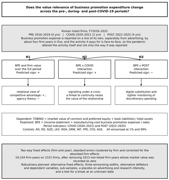
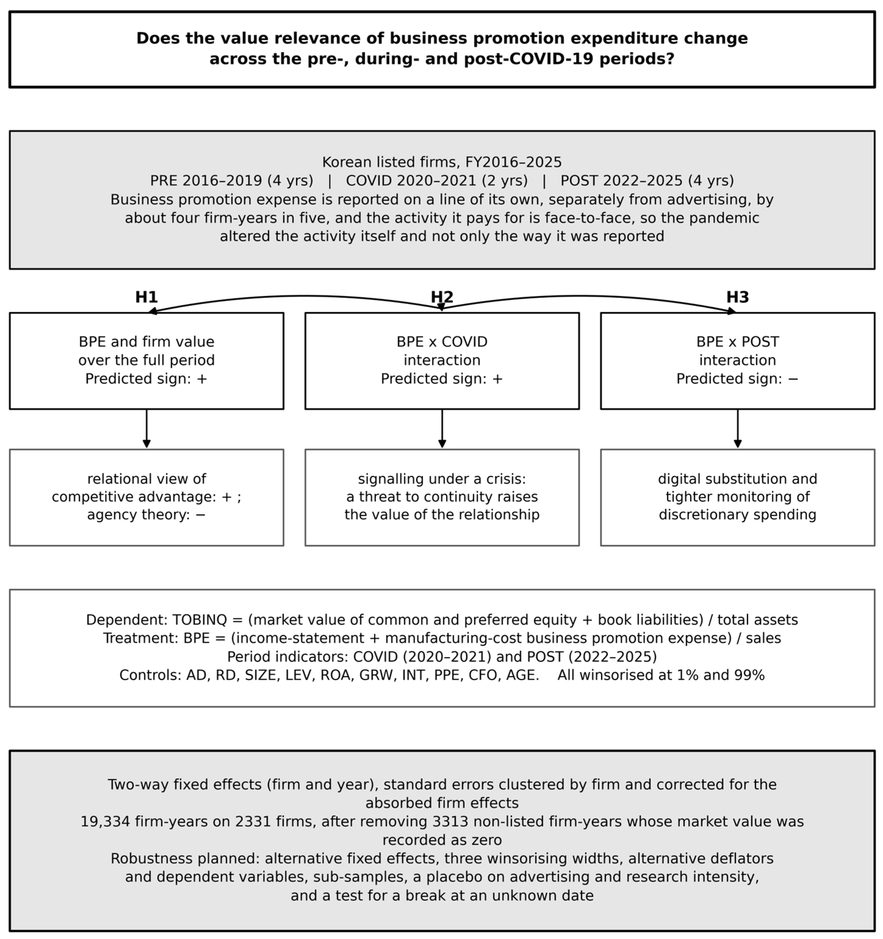
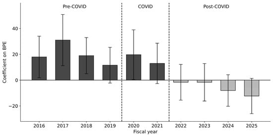
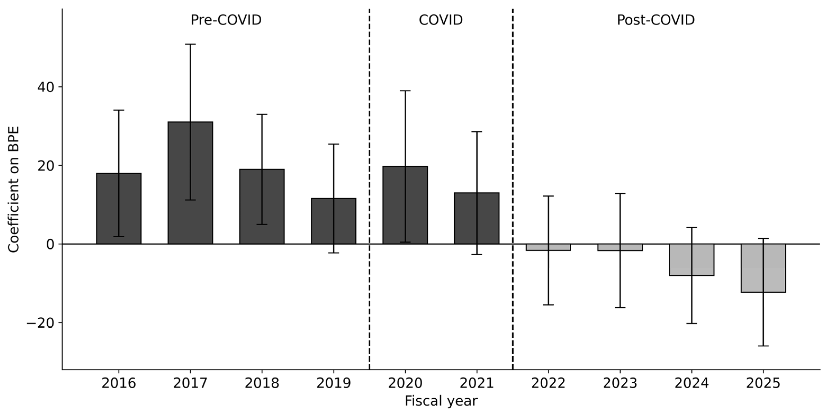
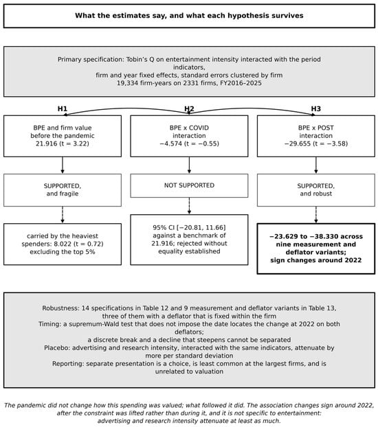
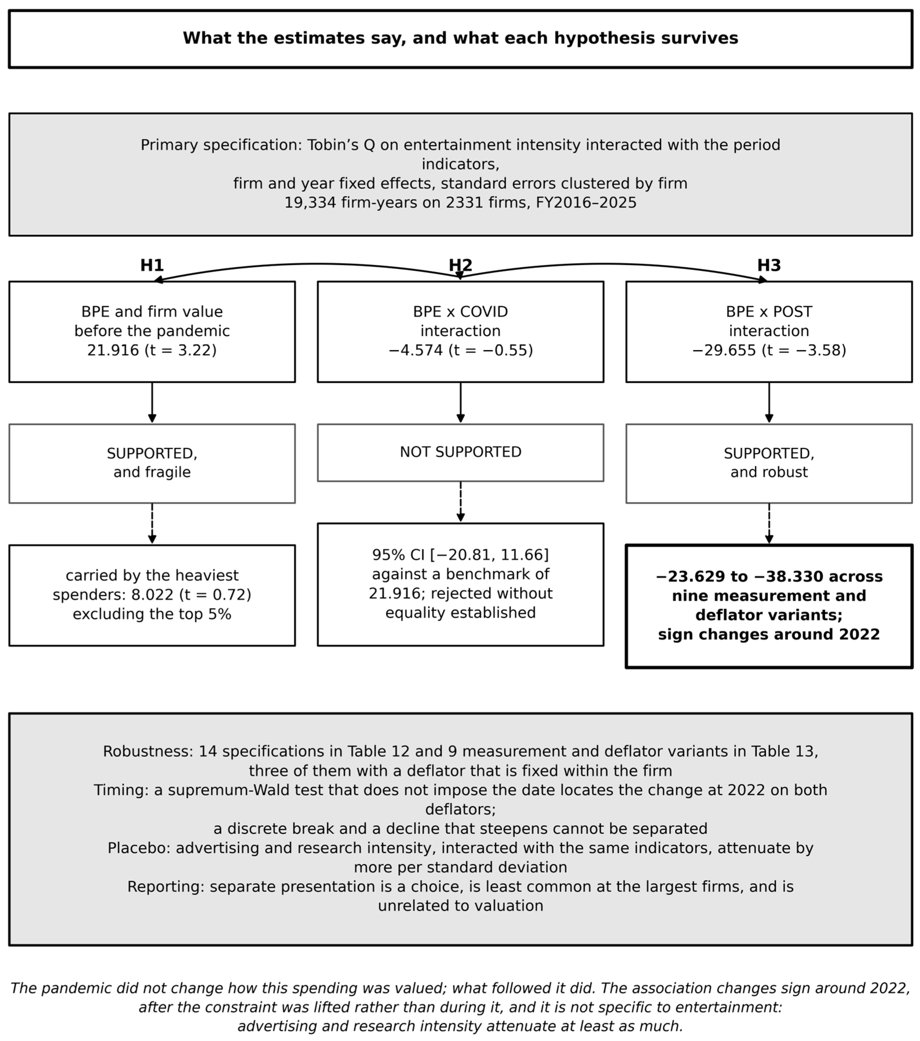

Disclaimer/Publisher’s Note: The statements, opinions and data contained in all publications are solely those of the individual author(s) and contributor(s) and not of MDPI and/or the editor(s). MDPI and/or the editor(s) disclaim responsibility for any injury to people or property resulting from any ideas, methods, instructions or products referred to in the content. |
© 2026 by the author. Licensee MDPI, Basel, Switzerland. This article is an open access article distributed under the terms and conditions of the Creative Commons Attribution (CC BY) license.