Selective Prediction and the Persistence Illusion: A Diagnostic Decomposition of VIX Regime Classification

Abstract

This paper develops a six-component diagnostic protocol for evaluating confidence-based selective prediction on autocorrelated financial labels, demonstrating it on VIX regime classification across 5000 trading days (July 2006–May 2026). The protocol combines coverage-matched baseline comparison, joint-coverage decomposition, regime-transition auditing, risk–coverage analysis, feature attribution, and abstention confound testing. Applied to Random Forest, Histogram Gradient Boosting, and XGBoost classifiers with 36 features, the protocol indicates that headline selective accuracy of 90–94% largely reflects label persistence: on jointly covered days, the Random Forest and a persistence rule calibrated on training data make identical predictions at three of five horizons (McNemar $b=c=0$) and disagree on at most 3 of 708 days elsewhere. All three classifiers and a forecast-then-threshold HAR model achieve 0% covered accuracy on calm-to-high transitions—across 16 distinct transition episodes at the shortest horizon—and an LSTM performs below chance on the same days. The pattern is consistent with an informational constraint of the daily feature set rather than a model deficiency, and it replicates on S&P 500 trend regimes. The protocol is modular and directly applicable to other selective prediction systems on serially correlated outcomes.

1. Introduction

Volatility is one of the most important dimensions of financial market risk. The CBOE Volatility Index (VIX), often described as the market’s “fear gauge,” summarizes option-implied expectations of S&P 500 volatility over the next 30 days and is widely used by investors, risk managers, and policymakers to monitor uncertainty in equity markets (Bekaert & Hoerova, 2014; Whaley, 2009). Elevated implied volatility is both a symptom and a propagation channel of macroeconomic uncertainty: uncertainty shocks generate sharp, clustered spikes in market fear with real-economy consequences (Bloom, 2009). When VIX rises above 20—a level widely adopted as a practical divide between normal and elevated-fear environments (Whaley, 2009)—markets are generally considered to be in a high-volatility regime characterized by elevated fear, widening credit spreads, and increased probability of large equity drawdowns. Episodes such as the COVID-19 crash of March 2020 and the Japan carry-trade unwind of August 2024 illustrate the costs of failing to anticipate these regime transitions.

Despite its importance, VIX regime prediction is a difficult problem. Volatility is noisy, mean-reverting, and driven by a complex mixture of market sentiment, equity conditions, interest rates, and sudden exogenous shocks. Classical approaches such as GARCH-family models (Bollerslev, 1986), realized-volatility frameworks (Andersen et al., 2003), and Markov-switching models (Hamilton, 1989) have provided important foundations, but often assume specific parametric structures that may not hold in practice, and macroeconomic predictors add surprisingly little to autoregressive volatility benchmarks out of sample (Paye, 2012). Machine learning methods offer flexibility in modeling nonlinear interactions across large feature sets, and have shown genuine promise in related asset-pricing applications (Gu et al., 2020), but they introduce their own challenges: temporal leakage, calibration, and—critically for regime classification—the difficulty of distinguishing genuine predictive skill from the strong autocorrelation inherent in VIX.

Before proceeding, a distinction is worth drawing explicitly: forecasting volatility itself (a continuous quantity, the object of the GARCH and HAR literatures) and forecasting binary volatility regimes (whether VIX will be above a threshold at a future date) are related but different problems. This paper is concerned with the latter—the classification task that underlies regime-based risk dashboards, allocation switches, and hedging triggers—and with how such classifiers should be evaluated.

The selective prediction literature—which studies classifiers that may abstain from uncertain predictions (Bartlett & Wegkamp, 2008; Chow, 1970; Geifman & El-Yaniv, 2017)—offers a principled approach to regime classification: reserve predictions for high-confidence cases and trading coverage for reliability on predicted days. On autocorrelated label sequences such as VIX regimes, however, selective prediction can manufacture the appearance of skill by preferentially covering easy regime-stable days. That persistence is hard to beat on autocorrelated financial series is well known; what is missing from the literature is a systematic way to determine whether—and precisely where—a given selective classifier adds anything beyond it.

The contribution of this paper is a six-component diagnostic protocol for making that determination, together with a detailed demonstration on VIX regime classification. The protocol comprises: (i) coverage-matched comparison against naive baselines calibrated on training data only; (ii) decomposition of the jointly covered prediction set by regime-transition type; (iii) transition-conditional accuracy auditing; (iv) threshold-free risk–coverage analysis; (v) feature attribution to detect autocorrelation exploitation; and (vi) abstention confound testing. Three ensemble classifiers—Random Forest (RF), Histogram Gradient Boosting (HGB), and XGBoost—are trained on 36 features and abstain when calibrated probability is close to 0.5.

Applied to this setting, the protocol indicates the following. First, headline selective accuracy of 90–94% is largely composition-driven: on jointly covered days, RF and a training-calibrated persistence rule make identical predictions at three of five horizons (McNemar $b=c=0$) and disagree on at most 3 of 708 shared days elsewhere; the aggregate accuracy gaps that do appear (significant only at $N=10$, $+2.8$ pp, 95% CI $[0.2,5.3]$) arise entirely from differences in which days each system covers. Second, a HAR-style logistic regression using only three features (current VIX level, 5-day VIX mean, 20-day VIX mean) is statistically indistinguishable from the full 36-feature RF at matched coverage (bootstrap CIs on the gap include zero), suggesting that the additional 33 features contribute little. Third, the confidence filter yields 0% accuracy on every covered calm→high transition—across 16 distinct transition episodes at $N=5$—for all three ensemble classifiers and for a forecast-then-threshold HAR model, while an LSTM performs below chance on the same days; explicit cost-weighting up to $20\times$ does not change this. Fourth, at $N=25$, balanced accuracy collapses to 50% for RF and HGB. Fifth, persistence at matched coverage dominates RF selective prediction on cost-weighted utility whenever false negatives are more costly than false alarms ($C\ge 5$) at $N=10$.

We state the scope of these claims carefully. The evidence presented here demonstrates the persistence illusion for two highly persistent financial classification problems (VIX regimes and S&P 500 trend regimes); the broader proposition—that selective prediction on any sufficiently autocorrelated label sequence is subject to the same artifact—is a hypothesis for which this study provides the first two supporting cases, not a demonstrated general property.

The remainder of the paper is organized as follows. Section 2 reviews related work. Section 3 describes the data. Section 4 presents the methodology. Section 5 reports empirical results. Section 6 replicates the diagnostic on S&P 500 trend regimes. Section 7 concludes.

2. Related Work

2.1. Volatility Forecasting and Regime Modeling

The modeling of financial volatility has a long history in econometrics. Bollerslev (1986) introduced the GARCH model, which captures the tendency of volatility to cluster over time by modeling conditional variance as a function of past squared residuals. GARCH-family models have since been extended in numerous directions and remain a standard benchmark for volatility forecasting. Hamilton (1989) introduced Markov-switching models, in which a time series is assumed to switch between discrete latent states according to a Markov chain. This framework provides a natural model for regime transitions and has been widely applied to financial and macroeconomic time series. Guidolin and Timmermann (2007) extended regime-switching ideas to multivariate portfolio allocation settings, demonstrating that regime-dependent models can outperform single-state specifications in out-of-sample asset allocation.

A complementary strand of work focuses on realized volatility constructed from high-frequency intraday returns (Andersen et al., 2003). Corsi (2009) proposed the Heterogeneous Autoregressive (HAR) model, which captures the long-memory properties of realized volatility through a simple additive structure of daily, weekly, and monthly volatility components. The HAR model has become a standard benchmark for realized volatility forecasting, and its strong performance motivates including a HAR-style logistic regression as a baseline in this paper.

In the VIX-specific literature, Whaley (2009) documented the VIX’s role as a fear indicator and its asymmetric behavior in market downturns. Bekaert and Hoerova (2014) decompose the VIX into a conditional-variance component and a variance risk premium, showing the two carry distinct information about risk appetite and uncertainty. Fernandes et al. (2014) studied the predictability of VIX using a variety of econometric models and found that simple autoregressive specifications perform competitively against more complex alternatives. This paper replicates and extends that finding: simple HAR-style models are competitive with 36-feature ensemble classifiers on the binary regime classification task.

2.2. Machine Learning for Financial Prediction

Machine learning methods have increasingly been applied to financial forecasting. Gu et al. (2020) provide the benchmark demonstration for empirical asset pricing, showing that tree ensembles and neural networks extract genuine predictive gains from large predictor sets. Ensemble methods such as Random Forests (Breiman, 2001) and Gradient Boosting are particularly well-suited to financial prediction because they can model nonlinear interactions among large feature sets without requiring distributional assumptions. The present paper’s message is complementary rather than contradictory to this literature: flexible models can add value, but on highly persistent classification targets their apparent gains require the kind of persistence-matched auditing developed here.

A key methodological challenge in applying machine learning to financial data is avoiding data leakage and respecting the temporal ordering of observations. This paper addresses this by using chronological train/test splitting, TimeSeriesSplit cross-validation during calibration, and walk-forward validation as a robustness check—consistent with best practices in applied financial machine learning.

2.3. Selective Prediction and the Reject Option

The reject option in classification allows a model to abstain from making a prediction when its confidence is insufficient. Chow (1970) first formalized the optimal reject option. Bartlett and Wegkamp (2008) studied classification with a reject option using hinge loss and established theoretical generalization bounds. Geifman and El-Yaniv (2017) demonstrated that selective prediction can substantially improve reliability in modern deep learning settings.

The subsequent literature has developed evaluation methodology specifically for selective classifiers. El-Yaniv and Wiener (2010) laid theoretical foundations for the risk–coverage trade-off, characterizing the achievable frontier between abstention rate and selective error. Geifman et al. (2019) proposed the area under the risk–coverage curve (AURC) as a threshold-free summary of selective performance, which is now a standard reporting convention. Fisch et al. (2022) extended calibration requirements to the selective setting, noting that confidence scores must remain calibrated conditional on coverage. This evaluative strand is directly relevant here: the diagnostic protocol we propose can be viewed as extending risk–coverage evaluation with components that are specifically needed when labels are serially correlated—transition-type decomposition, joint-coverage-composition analysis, and persistence-matched baselines.

In financial applications, the reject option is particularly natural. A risk model that provides no signal on ambiguous days is often more useful than one that forces a low-confidence prediction. However, on autocorrelated series such as VIX regimes, abstention can manufacture accuracy without genuine predictive skill—the central diagnostic this paper examines.

3. Data

3.1. Market Data

Daily price data are obtained from Yahoo Finance for eight market series: the CBOE Volatility Index (VIX), the 3-month VIX term structure index (VIX3M), the CBOE 9-Day Volatility Index (VIX9D), the S&P 500 Index, gold futures (GC=F), the 10-Year Treasury yield (TNX), the U.S. Dollar Index (DXY), and the CBOE SKEW Index. VIX9D is downloaded to keep the raw data complete but is not used as a model feature. Although raw VIX data is available from January 1990, VIX3M data begins in July 2006; because VIX3M anchors the term spread feature, the effective sample starts on 17 July 2006.

3.2. Macroeconomic Data

Two macroeconomic variables are obtained from the Federal Reserve Economic Data (FRED) API: the Federal Funds Rate and the 10-Year minus 2-Year Treasury yield curve spread (T10Y2Y). The Federal Funds Rate target is forward-filled to daily frequency by holding the prevailing rate constant between FOMC meeting dates.

3.3. Label Construction

The prediction task is binary regime classification. For a prediction horizon N, the label is

$${\mathrm{LABEL}}_{N,t}=\left\{\begin{array}{cc}1\hfill & \mathrm{if}{\mathrm{VIX}}_{t+N}\ge 20\hfill \\ 0\hfill & \mathrm{if}{\mathrm{VIX}}_{t+N}<20\hfill \end{array}\right.$$

(1)

The label is forward-shifted N days to ensure that all features are observed at time t and the outcome is measured at time $t+N$, eliminating lookahead bias. Horizons of $N\in \{5,10,15,20,25\}$ trading days are evaluated.

The threshold of 20 follows the long-standing practitioner convention documented by Whaley (2009): it sits close to the long-run VIX median, is the level most commonly used in industry commentary and risk dashboards to separate “normal” from “elevated-fear” environments, and is embedded in numerous volatility-targeting product rules. It is nonetheless a convention rather than a structural break point, so robustness at thresholds of 18 and 22 is reported in Appendix B, and we note that data-driven threshold selection (e.g., from a fitted regime-switching model) is a reasonable alternative that would change class prevalence but not the diagnostic design.

A sustained-high label is also constructed:

$${\mathrm{SUSTAINED}\_\mathrm{LABEL}}_{N,t}=\left\{\begin{array}{cc}1\hfill & \mathrm{if}{\mathrm{VIX}}_{t+k}\ge 20\mathrm{for}\mathrm{all}k\in \{1,\dots ,N\}\hfill \\ 0\hfill & \mathrm{otherwise}\hfill \end{array}\right.$$

(2)

3.4. Class Distribution and Train/Test Split

The full feature dataset covers 5000 trading days from 17 July 2006 to 29 May 2026. Data are split chronologically, with the first 80% used for training (2006–2022) and the remaining 20% for testing (2022–2026), preserving strict temporal ordering. Table 1 reports the resulting sample sizes and class balance at each prediction horizon.

Table 1. Sample sizes and class distribution (fraction of days with VIX ≥ 20) by prediction horizon after label shifting. The usable sample shrinks slightly with N because the final N days of the series have no observable label.

N	Train N	Test N	Train VIX ≥ 20	Test VIX ≥ 20
5	3996	999	36.7%	30.1%
10	3992	998	36.7%	30.1%
15	3988	997	36.8%	30.0%
20	3984	996	36.8%	29.9%
25	3980	995	36.9%	29.8%

High-volatility days are substantially less common in the test period (≈30%) than in training (≈37%), reflecting that the training window encompasses several high-volatility crises—the 2008–09 financial collapse, the 2011 eurozone episode, and the COVID-19 crash—whereas the test window is dominated by the post-bear-market recovery despite the elevated volatility of the first half of 2022. The majority-class (always-calm) baseline therefore achieves approximately 70% accuracy on the test window before any model is fit.

4. Methodology

4.1. Feature Engineering

The model uses 36 engineered features grouped into five categories. All features are computed using only information available at or before the prediction date t.

VIX technical indicators (13 features): 10-day and 20-day simple moving averages (SMA10, SMA20); 10-day and 20-day momentum; 10-day and 20-day rate of change; Bollinger Band standard deviation, upper and lower bands, and position within the band; 14-day RSI; moving-average cross (SMA10 − SMA20); and VIX term spread (VIX3M − VIX).

SKEW features (3 features): SKEW level, 5-day change, and 20-day change.

S&P 500 features (7 features): 1-day, 5-day, and 20-day returns; 10-day and 20-day price momentum; 20-day realized volatility; and 252-day maximum drawdown.

Cross-asset features (9 features): Gold 1-day, 5-day, and 20-day returns; 10-Year Treasury yield 1-day, 5-day, and 20-day changes; DXY 1-day, 5-day, and 20-day returns.

Macroeconomic features (4 features): Federal Funds Rate 1-month and 3-month changes; yield curve spread 1-month and 3-month changes.

The complete feature list appears in Appendix A.

4.2. Models and Training Pipeline

Three ensemble classifiers are evaluated: Random Forest (RF) and Histogram Gradient Boosting (HGB), both implemented via scikit-learn, and XGBoost (Chen & Guestrin, 2016). All use a single fixed specification: RF with n_estimators=200, max_depth=10, and min_samples_leaf=5; HGB with max_iter=200, max_depth=5, and learning_rate=0.1; XGBoost with n_estimators=200, max_depth=6, learning_rate=0.1, subsample=0.8, and colsample_bytree=0.8. All seeds set to random_state=42. Using one specification eliminates pipeline inconsistencies and provides a fair comparison across tables. All features are standardized using StandardScaler fit on the training set and applied to the test set. XGBoost is run through the identical pipeline (same features, split, calibration, and abstention rule) so that its transition-level behavior is directly comparable to RF and HGB.

4.3. Probability Calibration

The selective prediction rule requires well-calibrated probability estimates. We apply isotonic regression calibration using CalibratedClassifierCV with 5-fold TimeSeriesSplit cross-validation on the full training set. The calibrated probability at time t is denoted as ${\widehat{p}}_t$, representing the estimated probability that VIX will be in a high-volatility regime at $t+N$.

4.4. Confidence-Based Selective Prediction

The selective classifier makes a prediction only when ${\widehat{p}}_t$ is sufficiently far from 0.5. For the confidence threshold $\tau \in (0,0.5)$, the prediction rule is

$${\widehat{y}}_t=\left\{\begin{array}{cc}1\hfill & \mathrm{if}{\widehat{p}}_t>0.5+\tau \hfill \\ 0\hfill & \mathrm{if}{\widehat{p}}_t<0.5-\tau \hfill \\ \mathrm{abstain}\hfill & \mathrm{if}0.5-\tau \le {\widehat{p}}_t\le 0.5+\tau \hfill \end{array}\right.$$

(3)

Accuracy is evaluated only on days where the model makes a prediction. Coverage is defined as the fraction of test days on which a prediction is made. The primary threshold is $\tau =0.25$.

5. Results

5.1. Main Accuracy Results

Table 2 reports baseline and selective accuracy, coverage, and balanced accuracy on covered days at $\tau =0.25$, and Table 3 reports precision, recall and F1 on the same covered days for the Random Forest.

Table 2. Baseline and selective ($\tau =0.25$) accuracy, coverage, and balanced accuracy on covered days. Gain = selective minus baseline in percentage points (pp).

N	RF Base	RF Sel	RF Gain	RF Cov	RF BalAcc	HGB Sel	HGB Gain	HGB Cov	HGB BalAcc
5	83.4%	91.9%	+8.5 pp	76.3%	88.4%	92.1%	+8.9 pp	71.1%	88.2%
10	79.5%	90.0%	+10.5 pp	60.1%	84.8%	92.2%	+13.6 pp	63.1%	86.1%
15	76.2%	90.0%	+13.8 pp	51.3%	83.9%	92.2%	+21.3 pp	36.0%	89.5%
20	76.8%	92.7%	+15.9 pp	31.7%	79.1%	94.8%	+22.2 pp	26.8%	84.1%
25	73.4%	90.3%	+16.9 pp	26.9%	50.0%	92.7%	+26.5 pp	19.2%	50.0%

Table 3. Extended metrics on covered days for Random Forest ($\tau =0.25$). At $N=25$, precision and recall are both 0% and balanced accuracy equals 50%, confirming that the model exclusively predicts the calm class at this horizon.

N	Selective Acc	Precision	Recall	F1	Balanced Acc
5	91.9%	86.5%	81.2%	83.8%	88.4%
10	90.0%	86.8%	73.8%	79.7%	84.8%
15	90.0%	89.8%	70.8%	79.2%	83.9%
20	92.7%	100.0%	58.2%	73.6%	79.1%
25	90.3%	0.0%	0.0%	0.0%	50.0%

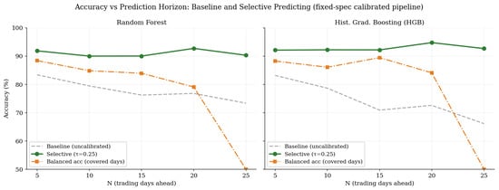
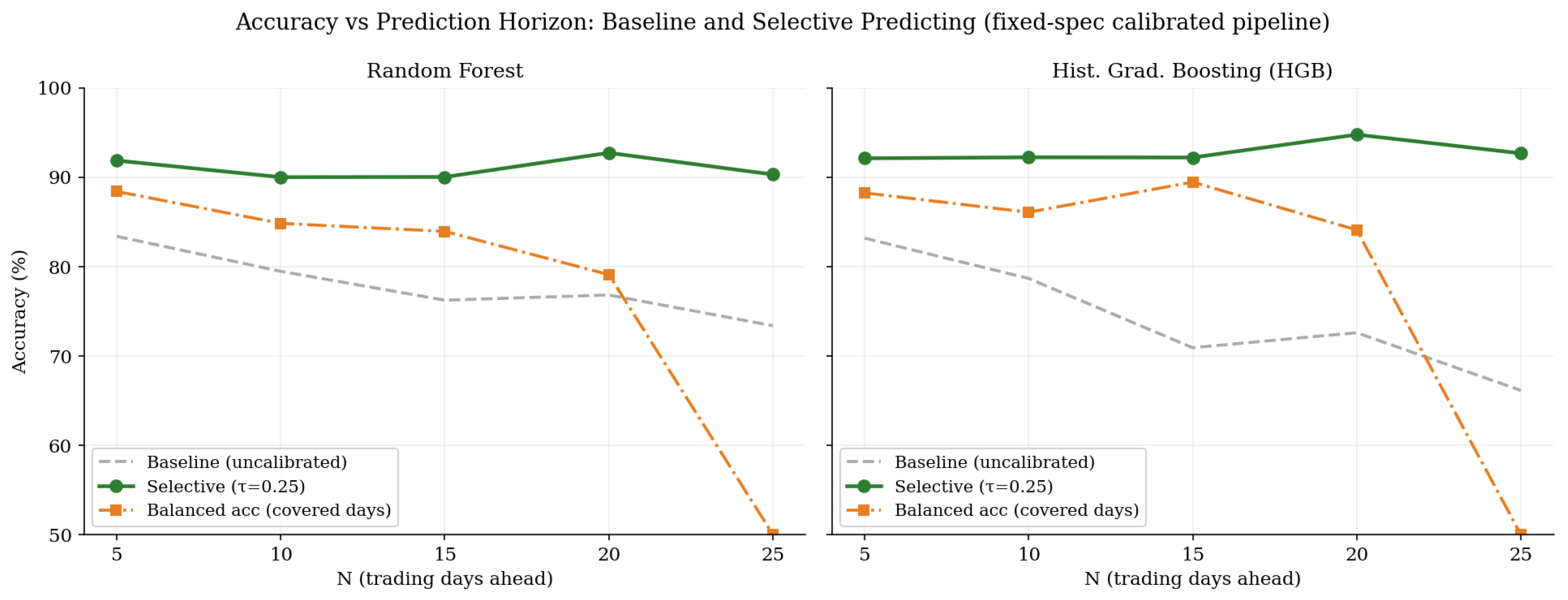
Figure 1 plots these results. Selective prediction improves accuracy for both models at every horizon. The balanced-accuracy columns, however, reveal the underlying artifact: RF balanced accuracy declines monotonically to 50.0% at $N=25$, indicating that the model exclusively predicts calm outcomes at the longest horizon—the nominal 90% selective accuracy there reflects the 70% base rate of calm days, not predictive skill.

Figure 1. Baseline, selective accuracy, and balanced accuracy across prediction horizons for Random Forest (left) and HGB (right). Baseline accuracy is computed on all test days; selective and balanced accuracy on covered days only. At $N=25$, balanced accuracy equals 50%, indicating a coin-flip result despite 90% selective accuracy.

5.2. Comparison to Naive Baselines

A critical question is whether the RF selective accuracy reflects genuine multi-feature ML skill or simply VIX autocorrelation. To answer this, we construct four coverage-matched baselines evaluated on the same test set.

The persistence baseline predicts ${\mathrm{VIX}}_{t+N}\ge 20$ if and only if ${\mathrm{VIX}}_t\ge 20$, and abstains when $|{\mathrm{VIX}}_t-20|<c$. The constant c is calibrated on the training window only: we compute the RF’s coverage rate on the training set at $\tau =0.25$ and select the smallest c whose training-window coverage matches it, then freeze c and apply it unchanged to the test window. No test-set information—neither labels nor VIX levels—enters the choice of c. The same protocol is used for every coverage-matched baseline below: each baseline’s abstention threshold is set as the quantile of its own training-window confidence distribution that reproduces the RF’s training coverage rate, then it is frozen. Because the thresholds are frozen before the test window is touched, realized test coverage rates differ modestly across systems (persistence covers 81.4% vs. the RF’s 76.3% at $N=5$, and 21.2% vs. 26.9% at $N=25$); we report both rates and address the composition of the covered sets directly in Section 5.10.

The LR (VIX only) baseline applies the full calibration pipeline to a single feature (current VIX level). The HAR-style logistic regression uses three features motivated by the HAR model (Corsi, 2009): current VIX (${\mathrm{VIX}}_D$), 5-day VIX mean (${\mathrm{VIX}}_W$), and 20-day VIX mean (${\mathrm{VIX}}_M$). The Markov-chain baseline estimates the 1-step transition probability matrix from training data and raises it to the Nth power.

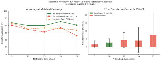
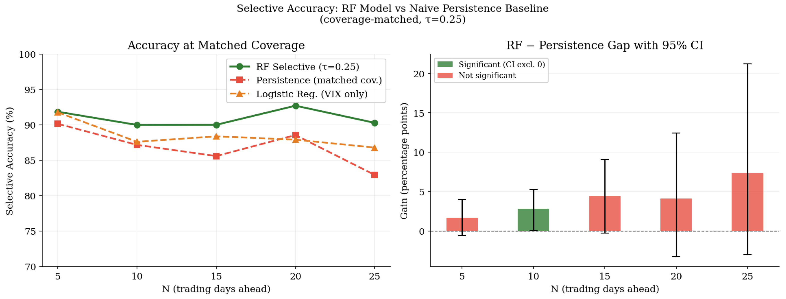
Three observations follow from Table 4 and Figure 2. First, the HAR-style logistic regression—using only three VIX-related features—remains within 1–4 pp of the full 36-feature RF at every horizon and exceeds it at $N=25$. A moving-block bootstrap on the HAR-minus-RF gap yields 95% CIs that include zero at both audited horizons ($N=5$: $[-3.46,+1.06]$; $N=10$: $[-4.65,+0.34]$), so the two systems are statistically indistinguishable despite the 12-fold difference in feature count. Second, the RF-minus-persistence gap is positive at all horizons but statistically significant only at $N=10$ ($+2.8$ pp, 95% CI $[+0.18,+5.27]$); Section 5.9 shows this gap is attributable to differences in which days the two systems cover, not to disagreement on shared days. Third, no baseline or model escapes the transition failure documented in Section 5.5 below.

Table 4. RF selective accuracy vs. naive baselines ($\tau =0.25$; all baseline abstention thresholds calibrated on the training window and frozen). All accuracies are computed on each system’s covered test days. Cov columns report realized test coverage. Bolded values indicate where a baseline exceeds the RF selective accuracy.

N	RF Cov	Persist Cov	Persistence	LR (VIX)	HAR-LR	Markov	RF Sel	RF − Persist
5	76.3%	81.4%	90.2%	91.8%	90.7%	83.7%	91.9%	+1.7 pp
10	60.1%	71.1%	87.2%	87.6%	87.8%	78.8%	90.0%	+2.8 pp
15	51.3%	64.1%	85.6%	88.4%	88.2%	70.0%	90.0%	+4.4 pp
20	31.7%	45.7%	88.6%	87.9%	90.3%	84.5%	92.7%	+4.2 pp
25	26.9%	21.2%	82.9%	86.8%	90.8%	82.9%	90.3%	+7.4 pp

Figure 2. (Left) RF selective vs. naive baseline accuracy across horizons (covered test days; baseline thresholds frozen from the training window). (Right) RF-minus-persistence gap with 95% moving-block bootstrap CI; only the $N=10$ interval excludes zero.

Why Not GARCH or Regime-Switching Benchmarks?

Two classical model families are deliberately absent from Table 4. GARCH-family models target the conditional variance of returns, a different object from the level of the option-implied VIX index; converting a GARCH variance path into a VIX threshold classification requires auxiliary assumptions about the variance risk premium that would make the comparison ambiguous. Fernandes et al. (2014) show that for the VIX level itself, simple autoregressive specifications are highly competitive, which is precisely the class our HAR-LR baseline (and the forecast-then-threshold HAR model below) represents. Markov-switching dynamics are represented directly by the Markov-chain baseline, which estimates regime-transition probabilities from training data. The next subsection adds the continuous-forecast route explicitly.

5.3. Forecast-Then-Threshold HAR and XGBoost Benchmarks

Because the regime label is a hard threshold at $\mathrm{VIX}=20$, one may ask whether the diagnostic structure of this paper is an artifact of discretizing a continuous, mean-reverting process—and whether a model that forecasts the VIX level first, and thresholds the forecast afterward, behaves differently. We therefore estimate a HAR regression of ${\mathrm{VIX}}_{t+N}$ on $({\mathrm{VIX}}_D,{\mathrm{VIX}}_W,{\mathrm{VIX}}_M)$ by least squares on the training window, predict the level at $t+N$, classify ${\widehat{y}}_t=\mathbf{1}[{\widehat{\mathrm{VIX}}}_{t+N}\ge 20]$, and abstain when the forecast is within a band d of the threshold, with d calibrated on training-window forecasts to match the RF’s training coverage and then frozen. Table 5 reports the result.

Table 5. Forecast-then-threshold HAR benchmark vs. RF selective accuracy, and its calm→high transition record. Accuracies on covered test days; the abstention band d is calibrated on the training window.

N	d	HAR-Thr Acc	HAR-Thr Cov	RF Sel	Calm→High Covered	Calm→High Acc
5	1.59	90.6%	78.7%	91.9%	38 of 79	0.0%
10	2.04	87.5%	71.1%	90.0%	41 of 101	0.0%
15	2.40	85.8%	63.7%	90.0%	40 of 104	0.0%
20	3.34	87.7%	45.6%	92.7%	15 of 105	0.0%
25	4.58	83.1%	22.0%	90.3%	8 of 115	0.0%

The forecast-then-threshold route reproduces the discrete pipeline’s behavior in full: overall covered accuracy within 1–7 pp of the RF, and 0% covered accuracy on calm→high transitions at every horizon. The mean-reverting HAR forecast, anchored on recent VIX levels, never projects a crossing from below 20 to above 20 with enough margin to clear the abstention band. This indicates the transition failure is not an artifact of binarization.

XGBoost, run through the identical pipeline, tells the same story from the model-complexity direction. Its selective accuracy (90.9–94.3% at $N\le 20$), coverage, and balanced-accuracy profile track the RF closely, including the balanced-accuracy collapse at $N=25$ (50.0%, with coverage shrinking to 2%). Its transition record is identical: 0% covered accuracy on calm→high days at all five horizons (covering between 1.7% and 45.6% of them), with 99–100% accuracy on regime-stable days. The full XGBoost table appears in Appendix C. Consistent with the informational-constraint interpretation, adding a third, stronger boosted architecture changes nothing about where the accuracy comes from.

5.4. Persistence Quantification

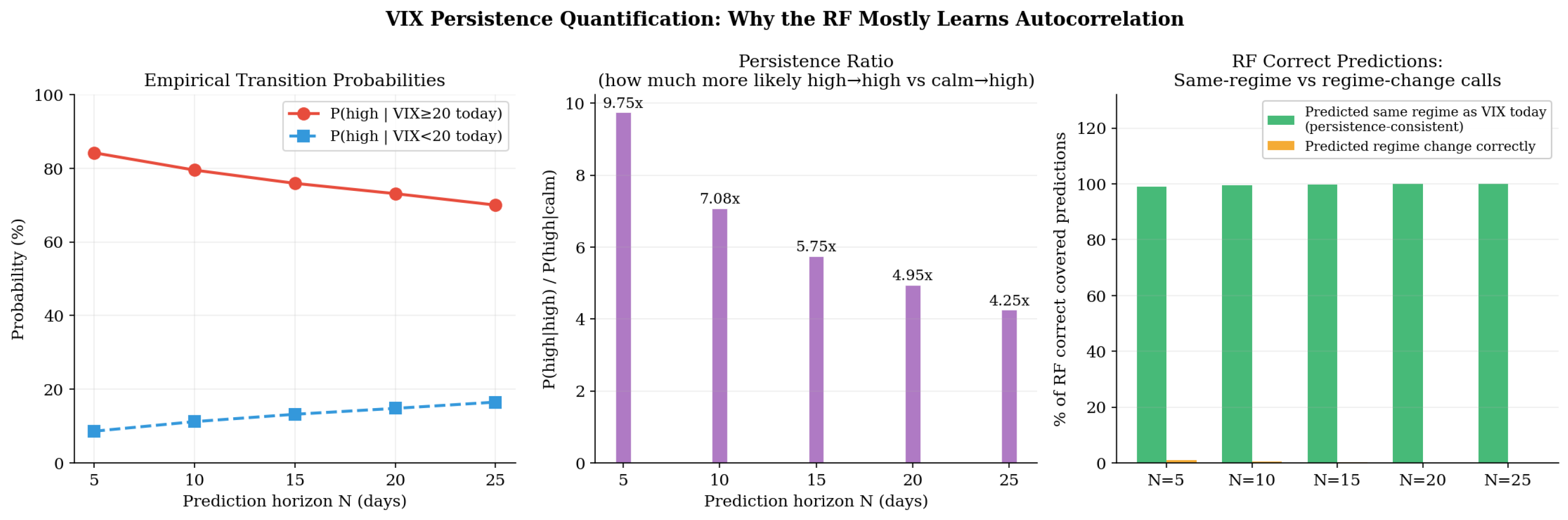
For each horizon N, we compute the empirical transition probabilities $Pr({\mathrm{VIX}}_{t+N}\ge 20\mid {\mathrm{VIX}}_t\ge 20)$ and $Pr({\mathrm{VIX}}_{t+N}\ge 20\mid {\mathrm{VIX}}_t<20)$, and classify each correct RF covered prediction as either a same-regime or regime-change call.

Figure 3 summarizes this decomposition. The persistence ratio—the relative probability of a high regime in N days conditional on today’s regime—reaches 9.75× at $N=5$, and the same-regime share of the RF’s correct covered predictions rises from 99.0% at $N=5$ to 100% at $N\ge 20$ (Table 6). On the days it chooses to cover, the RF adds no directional forecasting beyond VIX autocorrelation.

Figure 3. (Left) empirical transition probabilities conditional on today’s regime (all test days). (Center) persistence ratio P(H∣H)/P(H∣C). (Right) decomposition of RF correct covered predictions into same-regime and regime-change calls. At $N\ge 20$, 100% of correct predictions are same-regime.

Table 6. Empirical VIX transition probabilities and decomposition of RF correct covered predictions. P(H∣H) = P(${\mathrm{VIX}}_{t+N}\ge 20\mid$${\mathrm{VIX}}_t\ge 20$); P(H∣C) = P(${\mathrm{VIX}}_{t+N}\ge 20\mid$${\mathrm{VIX}}_t<20$). Same-regime % = fraction of correct RF covered predictions that match the regime at t.

N	P(H∣H)	P(H∣C)	Persist. Ratio	RF Cov. Acc	Same-Regime %
5	84.2%	8.6%	9.75×	91.9%	99.0%
10	79.5%	11.2%	7.08×	90.0%	99.6%
15	75.9%	13.2%	5.75×	90.0%	99.8%
20	73.1%	14.8%	4.95×	92.7%	100.0%
25	70.0%	16.5%	4.25×	90.3%	100.0%

5.5. Regime-Transition Analysis

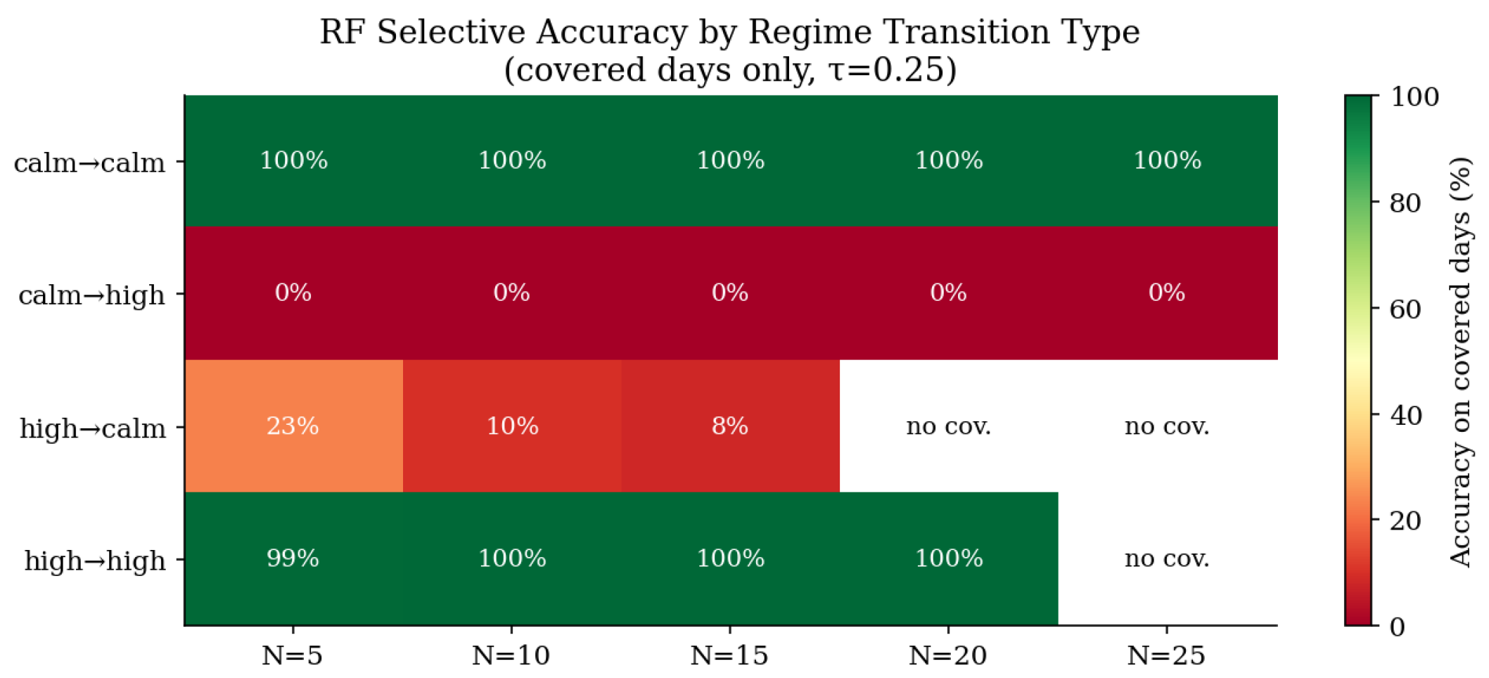
We classify each test day by the regime at time t and the realized regime at $t+N$, creating four transition categories: calm→calm, calm→high, high→calm, and high→high. Table 7 reports coverage and accuracy within each category, and Figure 4 plots them across horizons.

Table 7. RF selective coverage and accuracy by regime-transition type ($\tau =0.25$, test set; accuracy on covered days within each transition type). Calm→high accuracy is 0% at all horizons: every covered prediction on a day about to spike is a confident “stay calm” signal.

Transition	$\mathit{N}=5$			$\mathit{N}=10$
	Days	Coverage	Acc (Covered)	Days	Coverage	Acc (Covered)
calm → calm	614	87.1%	99.6%	587	71.6%	100.0%
calm → high	79	45.6%	0.0%	101	41.6%	0.0%
high → calm	84	35.7%	23.3%	111	18.0%	10.0%
high → high	222	72.5%	99.4%	199	59.3%	100.0%

Figure 4. RF selective accuracy by regime-transition type and horizon (covered days only, $\tau =0.25$). Calm→high rows are uniformly 0% at all horizons.

At $N=5$, the model covers 36 of 79 calm→high days (45.6%). On every single one of those 36 days, it issues a confident “stay calm” prediction and is wrong. The mechanism is clear: VIX comfortably below 20 generates calibrated probabilities below 0.25, triggering a high-confidence calm prediction.

5.5.1. How Many Independent Events Does the 0% Rest on?

Because transition days cluster around volatility episodes, day counts overstate the number of independent observations. Grouping the covered calm→high days into episodes (a gap of more than 10 trading days starts a new episode), the 0% record at $N=5$ spans 16 distinct episodes between August 2022 and January 2026—including the August 2022 bear-market rally failure, the February 2023 repricing, the October 2023 rate scare, the July–August 2024 carry-trade unwind, and the September–October 2025 and January 2026 spikes. The corresponding counts are 15 episodes at $N=10$, 12 at $N=15$, and 4–5 at $N=20$ and 25. At short horizons, the transition failure is therefore replicated across a substantial number of independent market events; at the two longest horizons the episode count is small, and the 0% figure there should be read as consistent with low—but not precisely estimated—transition skill.

5.5.2. Structural Caveat

This failure is not a model-specific defect: it is an expected structural property of the prediction problem. Calm→high transitions are disproportionately triggered by exogenous events—geopolitical shocks, central bank surprises, sudden liquidity dislocations—whose onset leaves no advance signature in publicly available daily price and macro-features. The diagnostic value of 0% covered accuracy is that the confidence filter fails to surface its own ignorance, issuing confident wrong predictions on covered transition days rather than abstaining.

5.5.3. Event Case Studies

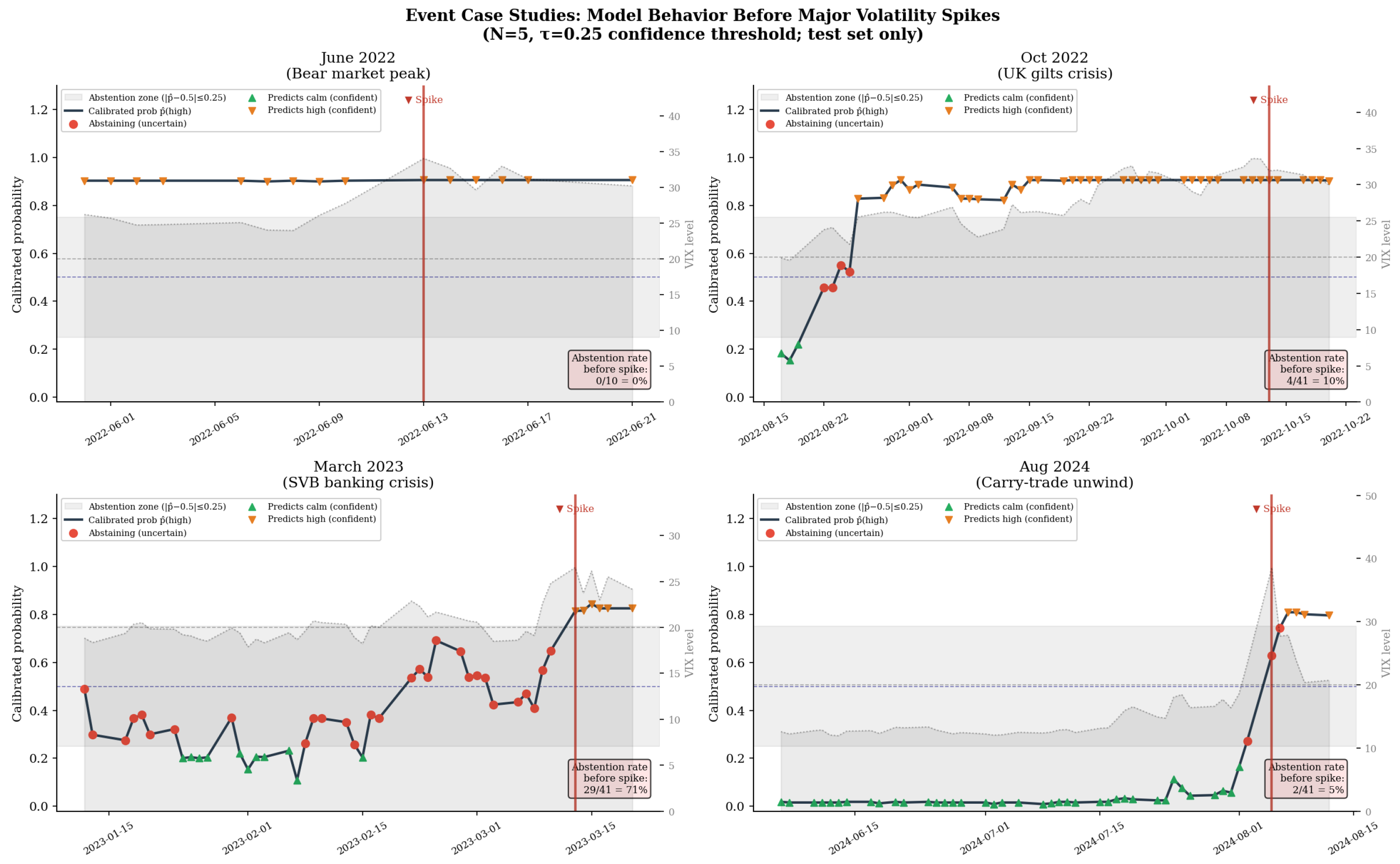
Figure 5 documents the model’s behavior during four major volatility events in the test set: the 2022 bear-market VIX peak (June 2022), the UK gilt crisis (October 2022), the SVB banking collapse (March 2023), and the Japan carry-trade unwind (August 2024, when VIX reached 65).

Figure 5. Model behavior (${\widehat{p}}_t$, $N=5$, $\tau =0.25$) for up to 40 trading days before four major volatility events (the June 2022 window is shorter because the test period begins in mid-2022). In all four cases the model issues confident calm predictions leading up to the event.

Across all four events the pattern is consistent: the model issues confident “stay calm” predictions on the days leading up to each spike. The August 2024 carry-trade unwind shows essentially no anticipatory signal; ${\widehat{p}}_t$ remains below $0.5-\tau$ until the day the spike materializes.

5.5.4. Cost-Weighting Does Not Rescue Calm→High Recall

To test whether the failure is informational rather than objective-function-driven, we refit the RF with explicit class weights $\{0:1,1:w\}$ for $w\in \{1,5,10,20\}$ (Table 8).

Table 8. Effect of class-weighting on transition coverage and selective accuracy. Calm→high accuracy is 0.0% at every weight for both horizons.

N	w	C→H Cov	C→H Acc	C→C Cov	C→C Acc	Sel Acc
5	1	45.6%	0.0%	87.1%	99.6%	91.9%
5	5	46.8%	0.0%	87.1%	100.0%	92.2%
5	10	49.4%	0.0%	87.3%	100.0%	92.3%
5	20	48.1%	0.0%	84.4%	100.0%	91.8%
10	1	41.6%	0.0%	71.6%	100.0%	90.0%
10	5	49.5%	0.0%	77.7%	100.0%	89.5%
10	10	58.4%	0.0%	80.4%	100.0%	87.4%
10	20	57.4%	0.0%	82.8%	100.0%	87.4%

The failure to predict calm→high transitions is informational with respect to this feature set, not objective-function-driven: no reweighting of the loss surfaces transition signal that the 36 daily features do not contain. Whether richer information sets—intraday options flow, news text, and macro surprise indices—could anticipate some transitions remains an open question we return to in the Limitations.

5.5.5. Abstention as a Leading Indicator

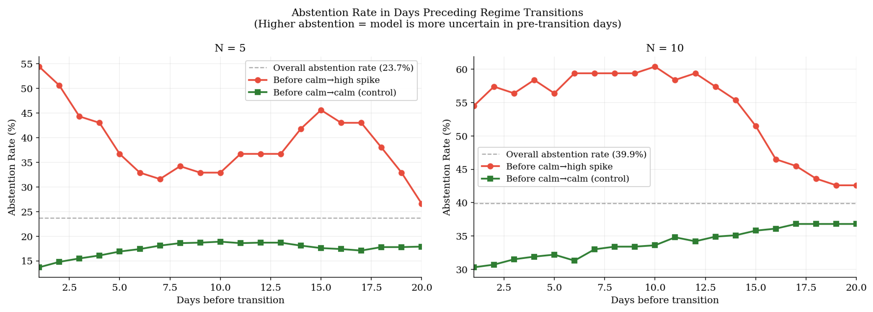
Figure 6 plots this. At $N=5$, the abstention rate immediately before a calm→high transition is 54.4%, compared to 13.7% before calm→calm days and 23.7% overall—a 2.3× elevation. However, a confound test shows that VIX proximity to the threshold (AUC $=0.805$) explains most of this signal; the abstention indicator alone achieves AUC $=0.708$. At $N=5$, abstention carries a small residual signal beyond proximity (likelihood-ratio $p=0.001$ on the evaluation sample, treated as descriptive rather than confirmatory). This observation should be treated as hypothesis-generating and requires dedicated out-of-sample confirmation.

Figure 6. Abstention rate (fraction of all test days on which the model declines to predict) before calm→high transitions (red) vs. calm→calm days (green). At lag = 1 day, the abstention rate before spikes is more than double the overall rate.

5.6. Walk-Forward Validation

Table 9 reports five-fold expanding walk-forward validation.

Table 9. Five-fold expanding walk-forward validation (fold means ± std of accuracy on each fold’s covered days; persistence threshold calibrated on each fold’s training window). Shaded rows indicate that at $N=20$ the RF/HGB standard deviations exceed 25 pp; persistence remains stable.

Model	N	Mean Baseline	Std	Mean Selective	Std
Random Forest	5	82.8%	9.7%	92.2%	1.7%
Persistence	5	88.0%	3.2%	92.7%	3.6%
HGB	5	84.0%	8.0%	84.6%	9.7%
Random Forest	10	72.3%	22.7%	85.9%	7.7%
Persistence	10	84.8%	4.5%	89.7%	5.0%
HGB	10	70.9%	22.9%	77.3%	15.2%
Random Forest	20	67.5%	22.8%	67.1%	28.3%
Persistence	20	81.5%	3.9%	84.5%	6.9%
HGB	20	63.6%	25.2%	61.4%	29.9%

Coverage-matched persistence at $N=5$ achieves 92.7% ± 3.6%—slightly higher mean than RF (92.2% ± 1.7%). At $N=10$, persistence (89.7% ± 5.0%) exceeds RF selective (85.9% ± 7.7%). At $N=20$, both RF and HGB show standard deviations exceeding 25 pp across folds, while persistence remains stable at 84.5% ± 6.9%. The practical reliable prediction window is approximately $N\le 10$.

5.7. LSTM Comparison

Table 10 compares the LSTM with the RF. A two-layer LSTM network is trained on sliding windows of the past 20 trading days of all 36 features, using the same 80/20 chronological split. The LSTM uses hidden size 64 and dropout 0.3 and is trained for 40 epochs with the Adam optimizer. The architecture was chosen as the standard recurrent sequence baseline in financial ML: two layers and hidden size 64 give roughly the parameter budget of the tree ensembles, the 20-day window matches the longest lookback in the engineered feature set (so the LSTM sees the same information horizon), and dropout 0.3 is a conventional regularization level for series of this length. We did not sweep architectures or window lengths; the LSTM’s role here is not to maximize sequence-model performance but to test whether temporal memory per se recovers transition signal that the static ensembles miss. Larger attention-based architectures are a direction for future work, though the results below suggest the constraint is informational rather than architectural.

Table 10. LSTM vs. RF at $\tau =0.25$. BalAcc = balanced accuracy on covered days. Both models are evaluated on the subsample of test days with a complete 20-day feature window, so the RF columns differ slightly from Table 2, which uses all test days.

N	LSTM Sel Acc	LSTM Cov	LSTM BalAcc	RF Sel Acc	RF Cov
5	76.5%	87.0%	76.0%	91.7%	77.0%
10	71.8%	90.7%	64.7%	89.3%	64.3%

The LSTM achieves non-zero calm→high covered accuracy (34.9% at $N=5$; 19.1% at $N=10$)—unlike the RF’s 0%—but both figures are substantially below the 50% random baseline, meaning the LSTM is wrong more often than right on transition days. Architectural richness (20-day temporal memory) does not resolve the information constraint: the daily feature set does not carry the event-anticipation content needed to forecast volatility spikes.

5.8. SHAP Feature Attribution

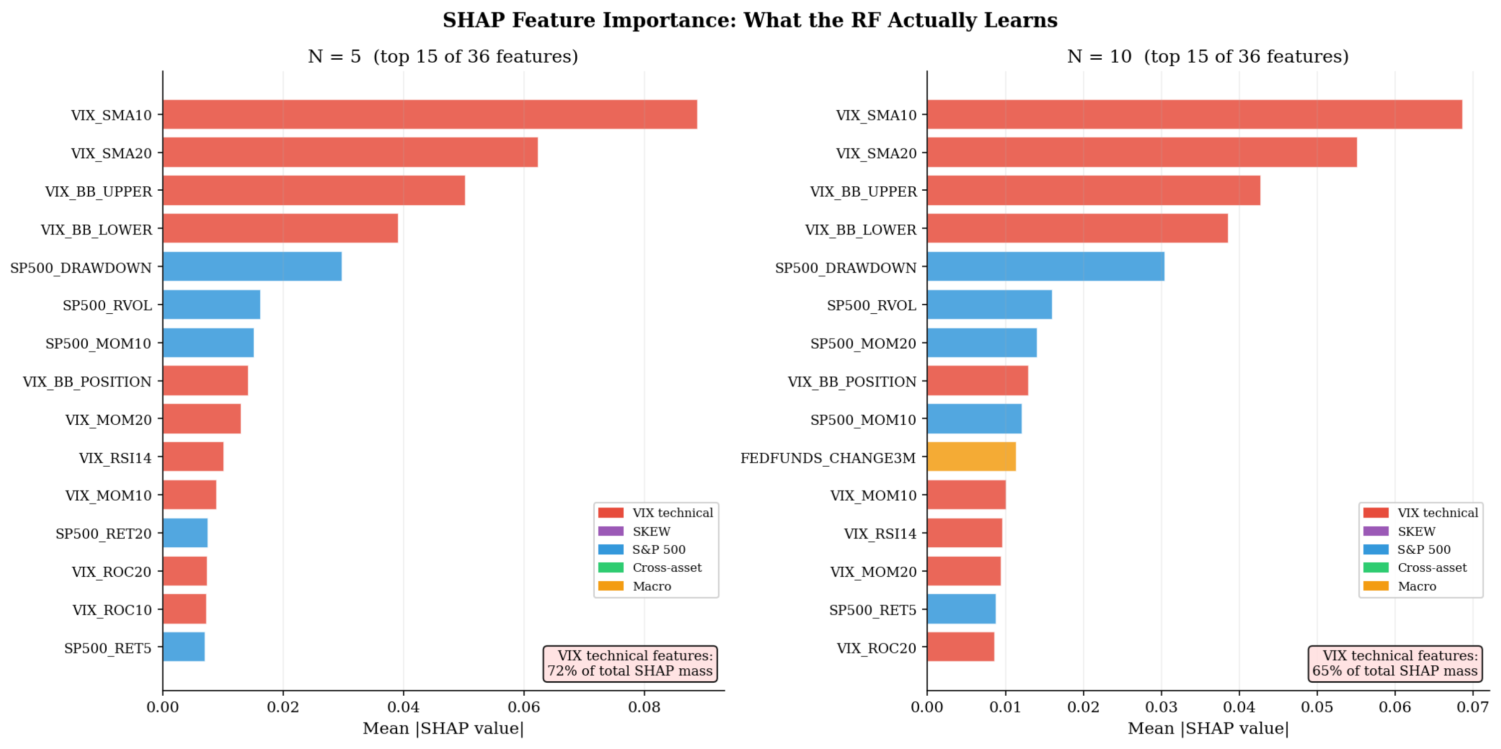
Figure 7 shows the attribution. VIX technical features account for 71.9% of total SHAP mass at $N=5$ and 64.7% at $N=10$. The dominant features are all smoothed or envelope transforms of the current VIX level. The SHAP decomposition is consistent with the model’s predictions being driven overwhelmingly by VIX autocorrelation, with negligible contribution from the broader cross-asset and macro-feature set. We note the standard caveat that SHAP values measure a model’s attribution of its own predictions, not causal importance (Lundberg & Lee, 2017): the analysis shows what the fitted model relies on and cannot rule out that the cross-asset features carry signal a differently specified model could exploit.

Figure 7. Mean absolute SHAP values (top 15 of 36 features) at $N=5$ (left) and $N=10$ (right). VIX technical features account for 71.9% and 64.7% of total SHAP mass, respectively.

5.9. Statistical Significance of the Persistence Gap

Table 11 reports the resulting intervals. We apply a moving-block bootstrap to the paired accuracy difference (RF selective minus persistence, with the persistence threshold frozen from the training window). The default block length is $max(\sqrt{N_{\mathrm{test}}},20)\approx 32$ days (Kunsch, 1989); 2000 bootstrap replicates are drawn. Because overlapping N-day-ahead labels induce serial dependence of order at least N in the loss differentials—on top of regime persistence that lasts far longer—we additionally re-run the bootstrap at block lengths of 60 and 90 days (Appendix D).

Table 11. Moving-block bootstrap 95% confidence intervals for the RF-minus-persistence selective accuracy gap (block length 32 days). Only the $N=10$ interval excludes zero; this holds at block lengths 60 and 90 as well (Appendix D).

N	Gap (pp)	95% CI Lower	95% CI Upper
5	$+1.70$	$-0.56$	$+4.12$
10	$+2.82$	$+0.18$	$+5.27$
15	$+4.42$	$-0.47$	$+9.15$
20	$+4.15$	$-3.09$	$+12.70$
25	$+7.36$	$-2.89$	$+20.71$

Four of five confidence intervals include zero; the exception is $N=10$, where the RF’s aggregate advantage of $+2.8$ pp is statistically significant. The McNemar test on jointly covered days clarifies what this aggregate gap does—and does not—consist of. At $N\in \{10, 20, 25\}$, RF and persistence make identical predictions on every jointly covered day ($b=c=0$, $p=1.000$). At $N=5$ they disagree on 3 of 708 jointly covered days and at $N=15$ on 1 of 462 (in the RF’s favor; $b=0$ in every case—persistence never beats the RF on a shared day—with $p\ge 0.08$ throughout). The significant $N=10$ aggregate gap therefore arises entirely from which days each rule covers: on the days both systems predict, their predictions coincide exactly. This is coverage-composition skill—the RF’s confidence score is a somewhat better abstention trigger than raw distance to the threshold—rather than predictive disagreement, and we quantify it directly in Section 5.10 and the risk–coverage analysis of Section 5.11. Excluding the 2022 bear-market period (149–165 test days) leaves all qualitative conclusions unchanged: calm→high covered accuracy remains 0% at all horizons.

5.10. Composition of the Jointly Covered Set

Matching coverage rates does not match which days are covered. To make the comparison concrete, Table 12 reports the size of the jointly covered set (days on which both the RF and the persistence rule predict) and its composition by transition type.

Table 12. Size and transition-type composition of the jointly covered set (RF ∩ persistence, $\tau =0.25$). Percentages in the four rightmost columns are shares of the joint set.

N	Joint Days	% of Test	RF Cov	Calm→Calm	Calm→High	High→Calm	High→High
5	708	70.9%	76.3%	70.9%	4.0%	3.1%	22.0%
10	556	55.7%	60.1%	70.3%	5.8%	3.1%	20.9%
15	462	46.3%	51.3%	70.6%	6.1%	2.6%	20.8%
20	257	25.8%	31.7%	83.3%	4.3%	0.0%	12.5%
25	113	11.4%	26.9%	92.9%	7.1%	0.0%	0.0%

The joint set is dominated by regime-stable days—92.9% at $N=5$ (calm→calm plus high→high) rising to 92.9% calm→calm alone at $N=25$—where not a single high→calm or high→high day survives both filters. We state the implication plainly: the $b=c=0$ result is close to guaranteed given the composition of the joint set—deep-calm and deep-high days on which any reasonable rule agrees. That is not a weakness of the analysis; it is the finding. The confidence filter and the distance-to-threshold rule select nearly the same easy days, which is precisely why selective accuracy is not evidence of skill beyond persistence on this task.

5.11. Risk–Coverage Analysis

Nearly all results above are reported at $\tau =0.25$. Following standard practice in the selective prediction literature (Geifman et al., 2019), Figure 8 reports full risk–coverage curves—selective error as a function of coverage, swept over the entire confidence range—for RF, HGB, XGBoost, and the persistence rule (whose confidence score is distance to the threshold, $|{\mathrm{VIX}}_t-20|$), with the area under the risk–coverage curve (AURC) in Table 13.

Figure 8. Risk–coverage curves per horizon (test set; selective risk = error rate on covered days as coverage varies over the full confidence sweep). Persistence uses $|{\mathrm{VIX}}_t-20|$ as its confidence score.

Table 13. Area under the risk–coverage curve (AURC; lower is better) by model and horizon.

N	RF	HGB	XGBoost	Persistence
5	0.049	0.060	0.053	0.056
10	0.083	0.081	0.087	0.104
15	0.107	0.123	0.130	0.130
20	0.109	0.124	0.120	0.146
25	0.146	0.147	0.161	0.206

The threshold-free view adds an honest nuance to the persistence story. The RF attains the lowest AURC at four of five horizons, and all three ML models rank their own confidence better than the distance-to-threshold heuristic over the full coverage range—the ML confidence ordering is genuinely more informative about which days are easy. However, this ranking advantage operates almost entirely within the regime-stable population: as Section 5.10 shows, at deployed coverage rates, the covered sets nearly coincide; as Section 5.5 shows, no ordering by confidence surfaces calm→high days as predictable. Better ranking of easy days does not translate into detection of the transitions that matter for risk management.

5.12. Cost-Weighted Utility Analysis

$$U=-{\displaystyle \frac{\mathrm{FP}+C·\mathrm{FN}}{n_{\mathrm{predictions}}}}$$

(4)

Table 14 reports the results. At $N=10$, persistence at matched coverage dominates RF selective prediction under any moderate false-negative cost asymmetry ($C\ge 5$). The RF selective framework is utility-beneficial only when false positives are as costly as false negatives ($C=1$).

Table 14. Cost-weighted utility per prediction under different FN/FP cost ratios C. Higher utility (closer to 0) is better. Bolded entries show where persistence dominates the RF selective classifier.

N	C	RF Selective	Persistence	RF Baseline	Always Calm
5	1	$-0.081$	$-0.087$	$-0.166$	$-0.301$
5	5	$-0.276$	$-0.286$	$-0.515$	$-1.507$
5	10	$-0.518$	$-0.535$	$-0.950$	$-3.013$
5	20	$-1.004$	$-1.033$	$-1.821$	$-6.026$
10	1	$-0.100$	$-0.120$	$-0.205$	$-0.301$
10	5	$-0.380$	$-\mathbf{0.326}$	$-0.626$	$-1.503$
10	10	$-0.730$	$-\mathbf{0.584}$	$-1.152$	$-3.006$
10	20	$-1.430$	$-\mathbf{1.100}$	$-2.204$	$-6.012$

6. Replication: S&P 500 Trend-Regime Classification

To test whether the persistence illusion is specific to volatility forecasting, we replicate the full diagnostic protocol on S&P 500 trend-regime classification using the same feature set and model specification. The label is

$${\mathrm{BEAR}}_{N,t}=\left\{\begin{array}{cc}1\hfill & \mathrm{if}{\mathrm{SP}500}_{t+N}<{\overline{\mathrm{SP}500}}_{200,t+N}\hfill \\ 0\hfill & \mathrm{otherwise}\hfill \end{array}\right.$$

(5)

The persistence baseline here predicts the current trend regime continues, with abstention when the S&P 500 is within a band of its 200-day moving average; the band is measured as a fraction of the moving average (so it is scale-free across the 2006–2026 index range) and is calibrated on the training window to match the RF’s training coverage, then it is frozen.

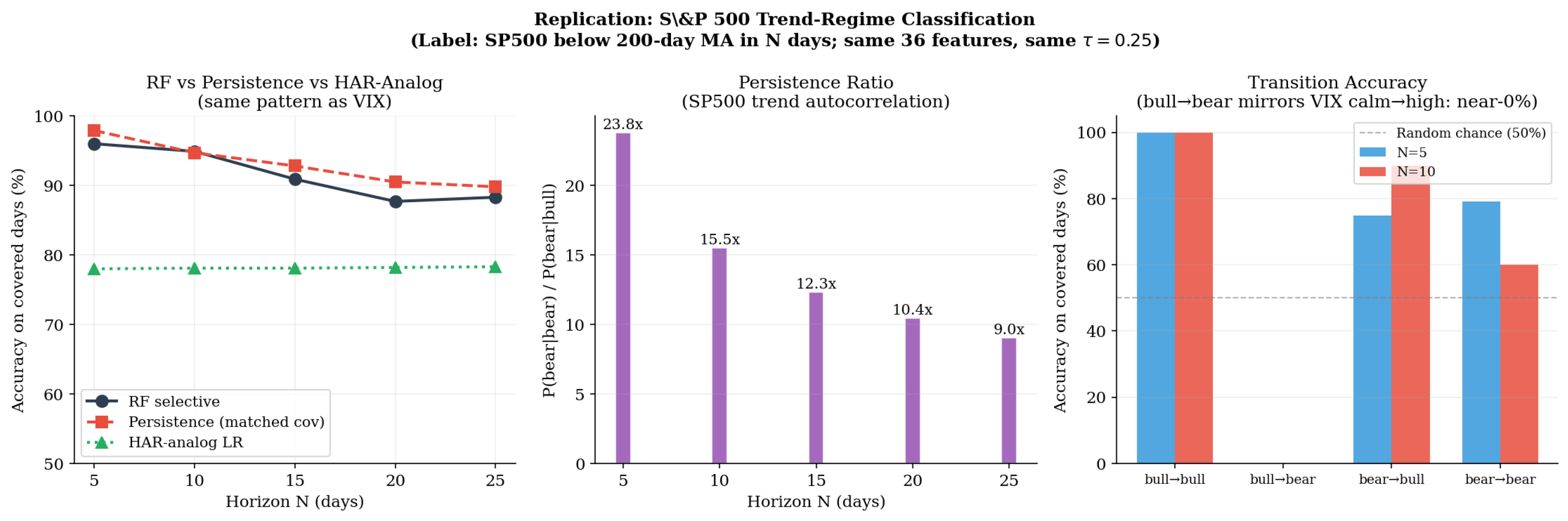
Table 15 reports the baseline comparison, Table 16 the transition breakdown, and Figure 9 summarizes both. The persistence ratio is 23.8× at $N=5$—more than twice the VIX ratio of 9.75×—and persistence matches or beats the RF at four of five horizons (RF−Persist: $-1.4$ to $-2.8$ pp, with a $+0.2$ pp tie at $N=10$). Note that the frozen persistence band covers more of the test window than the RF (roughly 90% vs. 60–74%), so its advantage is not an artifact of retreating to an easier covered subset: persistence predicts on more days, including harder ones, and still matches or exceeds the RF. Bull→bear covered accuracy is 0.0% at both $N=5$ and $N=10$, replicating the VIX calm→high finding exactly, and RF balanced accuracy again degrades toward 50% as the horizon grows. The replication is consistent with the persistence illusion being a structural consequence of applying selective prediction to highly autocorrelated binary time series rather than a VIX-specific artifact, though we emphasize that the two markets constitute supporting evidence for that broader hypothesis, not a demonstration of it.

Table 15. S&P 500 trend-regime replication (persistence band calibrated on training window). Accuracies on each system’s covered test days. RF−Persist is negative at four of five horizons: persistence matches or dominates the RF selective classifier.

N	Base Rate	RF Cov	Persist Cov	Persistence	HAR-Analog	RF Sel	RF−Persist
5	22.0%	74.4%	91.5%	97.9%	78.0%	96.0%	$-2.0$ pp
10	21.9%	68.3%	90.8%	94.7%	78.1%	94.9%	$+0.2$ pp
15	21.9%	69.7%	91.1%	92.8%	78.1%	90.9%	$-1.9$ pp
20	21.8%	70.3%	91.4%	90.5%	78.2%	87.7%	$-2.8$ pp
25	21.7%	59.5%	89.5%	89.8%	78.3%	88.3%	$-1.4$ pp

Table 16. S&P 500 transition accuracy. Bull→bear covered accuracy is 0%—exact mirror of VIX calm→high.

N	Transition	Days	Coverage	Acc (Covered)	Same-Regime %
5	bull→bull	749	88.8%	100.0%	99.2%
5	bull→bear	25	68.0%	0.0%
10	bull→bull	730	86.2%	100.0%	98.6%
10	bull→bear	39	71.8%	0.0%

Figure 9. S&P 500 trend-regime replication (covered test days; persistence band frozen from the training window). (Left) RF vs. persistence selective accuracy—persistence matches or dominates at four of five horizons. (Center) persistence ratio of 23.8× at $N=5$. (Right) bull→bear covered accuracy is 0%, replicating the VIX calm→high finding.

7. Conclusions

The primary contribution of this paper is a six-component diagnostic protocol for evaluating selective prediction systems on serially correlated labels, demonstrated in detail on VIX regime classification. Applied to this task, the protocol indicates that headline selective accuracy of 90–94% largely reflects label persistence rather than multi-feature machine learning skill. The evidence divides into two tiers, which we state separately.

Statistically supported findings. On jointly covered days, RF and a training-calibrated persistence rule make identical predictions at $N\in \{10,20,25\}$ (McNemar $b=c=0$) and disagree on at most 3 of 708 shared days at the remaining horizons, with persistence never winning a disagreement. The moving-block bootstrap on the RF-minus-persistence gap includes zero at four of five horizons (robust to block lengths of 32–90 days); the one significant gap ($N=10$, $+2.8$ pp) is attributable to coverage composition, since predictions on shared days coincide exactly. The HAR-minus-RF bootstrap CIs include zero at both audited horizons. The confidence filter achieved 0% covered accuracy on calm→high transitions at every horizon, across 16 independent transition episodes at $N=5$—for RF, HGB, XGBoost, and a forecast-then-threshold HAR model, with an LSTM performing below chance on the same days—and explicit cost-weighting up to $20\times$ did not change this.

Descriptive observations. Point-estimate patterns—the HAR-LR exceeding the RF at $N=25$, the ordering among baselines within overlapping confidence intervals, and the 1–7 pp spreads in Table 4—are reported as descriptive and should not be read as confirmed effects. We note that many comparisons are performed across horizons and analyses; because the paper’s central claims are negative results (absence of significant gaps), multiplicity concerns cut against finding spurious significance rather than in favor of our conclusions, but the descriptive tier should be interpreted accordingly.

The scope of the evidence is two highly persistent financial classification problems: VIX regimes and S&P 500 trend regimes. The proposition that the persistence illusion afflicts selective prediction on autocorrelated labels generally is a hypothesis these two cases support, not a demonstrated property; additional domains are needed before broader claims can be made.

7.1. Practical Implications: Who Should Use This Protocol and How

The protocol is designed for four audiences. Model validators and model risk management teams evaluating internal or vendor regime-classification signals can apply it to determine whether a marketed accuracy figure survives persistence-matched comparison. Quantitative researchers developing selective classifiers on financial time series can use it to locate where their model’s accuracy comes from before claiming skill. Referees and editors reviewing selective-prediction papers on autocorrelated data can use it as a review checklist. Practitioners deciding whether to deploy a regime signal can use the transition-level decomposition to see whether the signal works on the days that drive hedging value.

Concretely, we recommend that any selective prediction system on serially correlated labels report: (i) balanced accuracy alongside selective accuracy; (ii) a persistence baseline whose abstention threshold is calibrated on training data only; (iii) the size and transition-type composition of the jointly covered set; (iv) transition-conditional coverage and accuracy; (v) risk–coverage curves and AURC rather than a single threshold; and (vi) attribution analysis identifying reliance on autocorrelation proxies. Absence of these six items leaves open the possibility that reported accuracy is composition-driven.

Selective prediction itself is not the villain of this analysis, and from a risk-management perspective there remain concrete situations where it adds value despite its inability to detect transitions. First, abstention as an uncertainty signal: the abstention rate itself carries modest leading-indicator content (rising to 54% immediately before calm→high transitions at $N=5$ in our sample), so a desk can treat a spike in abstentions—rather than the model’s directional calls—as a trigger to review hedges, tighten position limits, or scale down volatility-sensitive exposure. Used this way, the system’s silence is the signal, and its silence is honest even when its predictions are not informative. Second, regime-stable confirmation: 99–100% covered accuracy on regime-stable days is genuinely useful for strategies whose main risk is acting on false alarms—for example, gating a systematic carry or volatility-selling program that should stay deployed in confirmed calm regimes and needs protection mainly against spurious exit signals. Third, avoiding forced low-confidence calls: in workflows where a model output feeds an automated decision, an abstention that routes the day to a human or to a conservative default is preferable to a forced coin-flip prediction. In each case the deployment principle is the same: use the selective system for what the diagnostic shows it can do (confirm continuation, flag its own uncertainty), and refuse to lean on it for what it cannot (anticipate spikes). What the protocol guards against is mistaking the accuracy of the covered subset for forecasting skill.

7.2. Limitations

The feature set consists of publicly available daily market data; the transition failure documented here is a statement about this information set, not about all possible information sets. Two of the feature groups (the CBOE SKEW index and the VIX term-structure spread) are themselves option-implied, so the negative result already covers the most accessible option-implied measures; richer sources—intraday options flow, macroeconomic surprise indices, news sentiment, textual and order-flow data—could in principle anticipate some exogenous transitions and are the primary open direction. Calm→high transitions are disproportionately triggered by exogenous shocks—geopolitical events, policy surprises, sudden liquidity crises—that leave no advance signature in daily price features. The four-year test period (≈1000 trading days) is underpowered for distinguishing accuracy differences of 1–3 pp under serial dependence, and contains 4–16 independent calm→high episodes depending on horizon. The replication spans two U.S. equity-linked markets; non-U.S. volatility indices (e.g., VSTOXX) and other asset classes remain untested.

7.3. Future Work

The primary open direction is feature enrichment: incorporating event-anticipation content such as options flow dynamics, credit spreads, news-based sentiment, or order-flow imbalance, to test whether the transition failure reflects the daily public information set or a deeper unpredictability of exogenous shocks. A two-stage system using the abstention rate as a leading indicator followed by a conditional spike-prediction model is a second natural direction. Third, the diagnostic protocol should be applied to additional autocorrelated regime classification tasks—credit spread regimes, recession prediction, and currency crisis indicators—to characterize how the persistence ratio relates to the severity of the selective-prediction bias and to test the generality of the persistence-illusion hypothesis.

Appendix B.1. Threshold Sensitivity

Table A2. Random Forest selective accuracy (covered days) and coverage as a function of confidence threshold $\tau$.

$\mathit{\tau }$	RF $\mathit{N}=5$ Acc	$\mathit{N}=5$ Cov	RF $\mathit{N}=10$ Acc	$\mathit{N}=10$ Cov
0.10	86.5%	91.0%	83.3%	90.5%
0.15	88.3%	85.1%	84.7%	85.9%
0.20	89.0%	82.9%	86.6%	78.5%
0.25	91.9%	76.3%	90.0%	60.1%
0.30	92.3%	73.6%	91.8%	53.6%
0.35	95.0%	67.1%	95.1%	36.5%
0.40	97.4%	49.0%	97.4%	15.3%

Table A2. Random Forest selective accuracy (covered days) and coverage as a function of confidence threshold $\tau$.

$\mathit{\tau }$	RF $\mathit{N}=5$ Acc	$\mathit{N}=5$ Cov	RF $\mathit{N}=10$ Acc	$\mathit{N}=10$ Cov
0.10	86.5%	91.0%	83.3%	90.5%
0.15	88.3%	85.1%	84.7%	85.9%
0.20	89.0%	82.9%	86.6%	78.5%
0.25	91.9%	76.3%	90.0%	60.1%
0.30	92.3%	73.6%	91.8%	53.6%
0.35	95.0%	67.1%	95.1%	36.5%
0.40	97.4%	49.0%	97.4%	15.3%

Accuracy increases monotonically with $\tau$ across all horizons, consistent with the calibrated probability being a reliable ranking signal. However, as Section 5.5 shows, increasing $\tau$ does not improve coverage of transition days—it makes confident wrong predictions on calm→high days even more selective.

Appendix B.2. Robustness Across VIX Thresholds

Table A3. Random Forest accuracy gain (selective accuracy on covered days vs. baseline accuracy on all days) by VIX regime threshold at $\tau =0.25$.

N	VIX ≥ 18	VIX ≥ 20	VIX ≥ 22
5	+5.4 pp	+8.5 pp	+7.5 pp
10	+11.3 pp	+10.5 pp	+10.3 pp
15	+14.8 pp	+13.8 pp	+7.9 pp
20	+22.3 pp	+15.9 pp	+9.1 pp
25	−14.8 pp	+16.9 pp	+8.3 pp

Table A3. Random Forest accuracy gain (selective accuracy on covered days vs. baseline accuracy on all days) by VIX regime threshold at $\tau =0.25$.

N	VIX ≥ 18	VIX ≥ 20	VIX ≥ 22
5	+5.4 pp	+8.5 pp	+7.5 pp
10	+11.3 pp	+10.5 pp	+10.3 pp
15	+14.8 pp	+13.8 pp	+7.9 pp
20	+22.3 pp	+15.9 pp	+9.1 pp
25	−14.8 pp	+16.9 pp	+8.3 pp

The advantage of selective prediction holds across VIX thresholds of 18, 20, and 22 at $N\le 20$. The exception is RF at $N=25$, VIX ≥ 18, which shows a gain of $-14.8$ pp, consistent with the degenerate behavior documented in Table 3.

Appendix B.3. Sustained Regime Labels

Table A4. Random Forest selective accuracy (covered days) for instantaneous and sustained regime labels at $\tau =0.25$.

N	Instantaneous	Sustained
5	91.9%	94.0%
10	90.0%	93.8%
15	90.0%	93.8%
20	92.7%	94.3%
25	90.3%	89.9%

Table A4. Random Forest selective accuracy (covered days) for instantaneous and sustained regime labels at $\tau =0.25$.

N	Instantaneous	Sustained
5	91.9%	94.0%
10	90.0%	93.8%
15	90.0%	93.8%
20	92.7%	94.3%
25	90.3%	89.9%

Sustained regime labels are consistently easier to predict than instantaneous labels at $N\le 20$, reflecting that persistent high-volatility episodes are preceded by stronger signals across multiple features.

References

- Andersen, T. G., Bollerslev, T., Diebold, F. X., & Labys, P. (2003). Modeling and forecasting realized volatility. Econometrica, 71, 579–625. [Google Scholar] [CrossRef] [Scilit]
- Bartlett, P. L., & Wegkamp, M. H. (2008). Classification with a reject option using a hinge loss. Journal of Machine Learning Research, 9, 1823–1840. [Google Scholar] [CrossRef] [Scilit]
- Bekaert, G., & Hoerova, M. (2014). The VIX, the variance premium and stock market volatility. Journal of Econometrics, 183, 181–192. [Google Scholar] [CrossRef] [Scilit]
- Bloom, N. (2009). The impact of uncertainty shocks. Econometrica, 77, 623–685. [Google Scholar] [CrossRef] [Scilit]
- Bollerslev, T. (1986). Generalized autoregressive conditional heteroskedasticity. Journal of Econometrics, 31, 307–327. [Google Scholar] [CrossRef] [Scilit]
- Breiman, L. (2001). Random forests. Machine Learning, 45, 5–32. [Google Scholar] [CrossRef] [Scilit]
- Chen, T., & Guestrin, C. (2016). XGBoost: A scalable tree boosting system. In Proceedings of the 22nd ACM SIGKDD international conference on knowledge discovery and data mining (pp. 785–794). ACM. [Google Scholar]
- Chow, C. K. (1970). On optimum recognition error and reject tradeoff. IEEE Transactions on Information Theory, 16, 41–46. [Google Scholar] [CrossRef] [Scilit]
- Corsi, F. (2009). A simple approximate long-memory model of realized volatility. Journal of Financial Economics, 7, 174–196. [Google Scholar]
- El-Yaniv, R., & Wiener, Y. (2010). On the foundations of noise-free selective classification. Journal of Machine Learning Research, 11, 1605–1641. [Google Scholar]
- Fernandes, M., Medeiros, M. C., & Scharth, M. (2014). Modeling and predicting the CBOE market volatility index. Journal of Banking & Finance, 40, 1–10. [Google Scholar] [CrossRef] [Scilit]
- Fisch, A., Jaakkola, T., & Barzilay, R. (2022). Calibrated selective classification. Transactions on Machine Learning Research. [Google Scholar]
- Geifman, Y., & El-Yaniv, R. (2017). Selective classification for deep neural networks. Advances in Neural Information Processing Systems, 30. [Google Scholar]
- Geifman, Y., Uziel, G., & El-Yaniv, R. (2019, May 6–9). Bias-reduced uncertainty estimation for deep neural classifiers. International Conference on Learning Representations (ICLR), New Orleans, LA, USA. [Google Scholar]
- Gu, S., Kelly, B., & Xiu, D. (2020). Empirical asset pricing via machine learning. The Review of Financial Studies, 33, 2223–2273. [Google Scholar] [CrossRef] [Scilit]
- Guidolin, M., & Timmermann, A. (2007). Asset allocation under multivariate regime switching. Journal of Economic Dynamics and Control, 31, 3503–3544. [Google Scholar] [CrossRef] [Scilit]
- Hamilton, J. D. (1989). A new approach to the economic analysis of nonstationary time series and the business cycle. Econometrica, 57, 357–384. [Google Scholar] [CrossRef] [Scilit]
- Kunsch, H. R. (1989). The jackknife and the bootstrap for general stationary observations. Annals of Statistics, 17, 1217–1241. [Google Scholar] [CrossRef] [Scilit]
- Lundberg, S. M., & Lee, S. I. (2017). A unified approach to interpreting model predictions. Advances in Neural Information Processing Systems, 30. [Google Scholar]
- Paye, B. S. (2012). ‘Déjà vol’: Predictive regressions for aggregate stock market volatility using macroeconomic variables. Journal of Financial Economics, 106, 527–546. [Google Scholar] [CrossRef] [Scilit]
- Whaley, R. E. (2009). Understanding the VIX. Junior Portfolio Manager, 35, 98–105. [Google Scholar] [CrossRef] [Scilit]
Disclaimer/Publisher’s Note: The statements, opinions and data contained in all publications are solely those of the individual author(s) and contributor(s) and not of MDPI and/or the editor(s). MDPI and/or the editor(s) disclaim responsibility for any injury to people or property resulting from any ideas, methods, instructions or products referred to in the content. |
© 2026 by the authors. Licensee MDPI, Basel, Switzerland. This article is an open access article distributed under the terms and conditions of the Creative Commons Attribution (CC BY) license.