


Abstract
Empirical evidence shows that the El Niño-Southern Oscillation (ENSO) influences the frequency–damage relationship for floods. However, ENSO is generally not incorporated into indemnity-trigger modeling of Flood Catastrophe Bonds (FCBs), resulting in an incomplete representation of claim events. Therefore, this study aims to develop an FCB pricing model that incorporates ENSO as an external systematic risk factor affecting the indemnity trigger. The trigger is formulated as a doubly stochastic compound Poisson process, with its intensity modeled as an autoregressive integrated moving-average with exogenous variables. Bond prices are then derived by integrating the trigger process with the Cox-Ingersoll-Ross model under an arbitrage-free risk-neutral framework. To obtain stable numerical solutions, a Monte Carlo-based algorithm is also developed. Numerical simulations using data from Bandung Regency, Indonesia, show stable estimates under the relative Monte Carlo standard error measure. Then, incorporating ENSO empirically improves flood-intensity forecasting accuracy, as indicated by lower MAPE, MAE, RMSE, and Theil’s U. It also produces statistically significant price differences across all common maturities. This study advances the theoretical and practical pricing of FCBs by directly linking climate-driven flood intensity to indemnity triggers, equipping practitioners to quantify risk better and to set sustainable disaster risk financing, particularly in ENSO-affected regions.
1. Introduction
Floods are among the most frequent and economically damaging disasters worldwide. Global economic losses from natural disasters exceed USD 300 billion annually, with floods accounting for a substantial share of these losses (Salhab & Rentschler, 2020). For instance, extreme flood events resulted in losses of approximately USD 80 billion in 2021 alone (Swiss Re Institute, 2023). The risk of economic losses and the frequency of flood events are projected to increase significantly in the future in line with the intensification of climate change and anthropogenic activities (Bhuyan et al., 2010; Hussain, 2011; Saf, 2009; W. Wang et al., 2013). In developing countries such as Indonesia, economic losses due to floods are expected to increase three to four times by 2050 compared to current conditions (Wijayanti et al., 2017). This increase in the scale and uncertainty of losses directly challenges the capacity of existing flood disaster financing systems (Januriyadi et al., 2018).
Flood loss financing to date has remained dominated by post-disaster government budgets and social assistance, with a limited share from conventional insurance. This approach becomes increasingly inadequate as economic losses rise and flood events occur more frequently. Limited allocation of state budget resources (Manzoor et al., 2022), high claim values (Ma & Ma, 2013), and relatively slow fund disbursement processes (Braun & Kousky, 2021) intensify fiscal pressure and delay economic recovery. These conditions indicate the need for more innovative, market-based financing mechanisms to manage flood risk sustainably (Cummins & Weiss, 2009; Loubergé et al., 1999).
In response, flood catastrophe bonds (FCBs), which are part of insurance-linked securities (ILS), have been developed with the support of the World Bank as one of these innovative instruments to transfer flood risk to global financial markets (Sukono et al., 2025). This instrument enables the provision of post-disaster financing that is relevant for strengthening government fiscal resilience. Under this instrument, part or all of the flood risk is transferred to bond investors who are willing to bear it. As compensation for bearing this risk, investors may receive higher returns than those offered by conventional bonds (Cummins, 2008; Cummins & Mahul, 2008). Several countries have begun to implement FCBs, such as New Zealand, which issued bonds through the New Zealand Earthquake Commission in May 2023 with a value of NZD 225 million, as well as Japan through Mitsui Sumitomo and Aioi Nissay Dowa Insurance Co., Ltd., with a value of USD 220 million (see more details at https://www.artemis.bm/deal-directory, accessed on 21 December 2025). However, although several countries have implemented FCBs, the fair pricing of this instrument remains an ongoing research issue. It is because the pricing process is determined not only by financial factors but also by concurrent flood risk. Under current conditions, this flood risk is strongly influenced by climate dynamics (e.g., the El Niño-Southern Oscillation, or ENSO). Therefore, a modeling approach that consistently links climate and financial risk is required (Burnecki et al., 2005; Cox & Pedersen, 2000).
Recent studies have increasingly incorporated climate risk into financial modeling frameworks. For example, Damette et al. (2026) showed that climate variability, especially ENSO, can act as an exogenous shock that affects banking sector stability through increased credit risk. Similarly, at the micro level, Zhang and Ming (2025) found that both physical and transition climate risks significantly increase bank risk-taking behavior. In the context of asset pricing, Lontzek et al. (2023) and Karydas and Xepapadeas (2022) developed models that incorporate climate risk into asset prices and interest rates through long-run risk and extreme events. Building on these developments, Agliardi and Agliardi (2021) extended bond pricing models by incorporating climate-related risks that affect firm value and credit quality. Complementing these modeling efforts, Acharya et al. (2024) provided empirical evidence that physical climate risk is priced across financial markets, including bonds and equities. Furthermore, Kling et al. (2021) showed that climate vulnerability can increase the cost of capital and limit firms’ access to finance. From a disaster risk perspective, Fan and Xiao (2023) developed a stochastic model that links disaster probability to asset return dynamics. Taken together, these studies show that climate risk is increasingly integrated into financial models through econometric, asset-pricing, and stochastic approaches.
Several studies have focused on developing quantitative pricing models for Flood Catastrophe Bonds (FCBs) as instruments for managing flood-related financial risks. J. Chen et al. (2013) developed an indemnity-index-based FCB pricing model using a Compound Poisson Process (CPP), with prices approximated from Chinese flood-loss data via the Wang double-factor method (S. S. Wang, 2004). Chao and Zou (2018) extended this approach by introducing multiple trigger indices, combining indemnity losses and total fatalities within a CPP–Peaks Over Threshold–Copula framework, and estimated prices using Monte Carlo simulation based on Chinese data. Li et al. (2022) proposed an index-based FCB pricing model driven by maximum rainfall, integrating a standard Poisson process with a Peaks Over Threshold (POT) approach and applying the Wang transform (S. S. Wang, 2000) due to the absence of a closed-form solution. More recent studies have expanded FCB modeling to different trigger structures and regional contexts. Ibrahim et al. (2023) formulated an indemnity-based FCB pricing model, with numerical solutions obtained using the approximation techniques proposed by Chaubey et al. (1998) and Reijnen et al. (2005). Sukono et al. (2024) proposed a rainfall-index-based FCB model that explicitly accounts for dry and rainy season durations in tropical regions, such as Indonesia, using a POT approach and moving-average smoothing. Sukono et al. (2025) further developed an FCB pricing framework based on indemnity and inundation-house indices, with bond prices estimated via Monte Carlo simulation. Collectively, these studies demonstrate the growing use of stochastic processes and simulation-based methods in FCB pricing, particularly in emerging and disaster-prone regions.
Despite these advances, a critical limitation remains in the existing FCB pricing literature. Current models, especially those based on indemnity triggers, assume that flood occurrence intensity is stationary and independent of large-scale climate dynamics. As a result, indemnity losses and trigger activation are typically modeled without explicitly accounting for systematic climate variability. This assumption is increasingly restrictive in the context of climate change, where large-scale climate phenomena such as the El Niño–Southern Oscillation (ENSO) have been shown to significantly alter regional rainfall patterns and flood intensity (Räsänen & Kummu, 2013; Ward et al., 2016). Empirical evidence further suggests that incorporating climate variables as covariates in flood-intensity models improves the estimation of extreme-event probabilities compared to stationary specifications (Zeng et al., 2021). From a public-sector disaster risk financing perspective, this omission is non-trivial. Public agencies rely on catastrophe bonds not only as financial instruments but also as decision-support tools for allocating resources, managing contingent liabilities, and planning long-term disaster risk strategies. Ignoring climate-driven shifts in flood risk may therefore lead to mispriced bonds and suboptimal financing decisions. Addressing this gap, the present study develops an indemnity-based FCB pricing framework that explicitly integrates ENSO-conditioned flood intensity into the modeling of cumulative flood losses. By linking large-scale climate signals to trigger activation and bond valuation, the proposed framework provides a more realistic and policy-relevant basis for public disaster risk financing, particularly in climate-vulnerable and emerging regions.
To operationalize ENSO-conditioned flood modeling, an appropriate representation of ENSO variability is required. Among the various indices used to represent ENSO, the Oceanic Niño Index (ONI) and Southern Oscillation Index (SOI) are considered the most representative, as they capture the key oceanic and atmospheric components of ENSO variability (Y. Chen et al., 2024; Wei, 2024). Physically, ONI reflects sea surface temperature anomalies that modulate energy availability and moisture supply through evaporation, while SOI represents atmospheric pressure gradients that regulate large-scale circulation and convection. Their combined use provides a more comprehensive representation of rainfall-generating mechanisms, particularly in controlling moisture availability and vertical atmospheric motion as key processes underlying extreme precipitation events. Empirically, ONI and SOI have been shown to exhibit significant associations with hydroclimatic extremes, including floods. Lam et al. (2019) demonstrated that ONI was significantly associated with increases in the number of people affected by floods, reflecting variations in both the frequency and intensity of flood events. In addition, Mera et al. (2018) reported that ONI and SOI were strongly correlated with hydrological variability. Comparative studies further indicate that these indices perform consistently with other ENSO representations, including multivariate indices such as the Multivariate ENSO Index (MEI) (Lam et al., 2019; Mohsin et al., 2026). Therefore, ONI and SOI are not only physically grounded but also empirically supported in explaining flood variability.
Addressing these limitations, this study develops a novel quantitative pricing framework for FCBs with an indemnity-based trigger under ENSO-conditioned flood intensity. The main theoretical contribution lies in the formulation of an integrated stochastic modeling structure that exogenously incorporates climate variability into both the flood-intensity process and the loss-generation mechanism. ENSO dynamics are represented by the ONI and SOI, which are summarized into annual indicators relevant to the insured region. Then, both are incorporated as external factors influencing the annual flood intensity process in an Autoregressive Integrated Moving-Average with Exogenous Variables (ARIMAX) framework. This specification extends existing FCB pricing models by explicitly allowing climate-driven non-stationarity in flood occurrence, rather than relying on the standard stationarity assumption. Based on the resulting ENSO-conditioned flood-intensity process, the indemnity trigger, measured by cumulative flood losses, is modeled as a doubly stochastic compound Poisson process (DSCPP). In this formulation, flood events arrive according to a stochastic intensity governed by climate-conditioned dynamics, allowing the model to capture time-varying event frequency while preserving a consistent representation of cumulative losses required for indemnity-based triggers. This choice is particularly suitable as it directly links climate-driven variability to loss accumulation without restricting the model to extreme events or self-exciting behavior. The resulting loss process is then embedded within a risk-neutral valuation framework to derive FCB prices as the present value of expected investor cash flows. For the discounting mechanism, the interest rate is modeled using a Cox-Ingersoll-Ross (CIR) process, which ensures non-negative rates and incorporates state-dependent volatility, providing a realistic representation of interest-rate uncertainty in long-term bond valuation. Together, these components define a unified theoretical framework that consistently integrates climate dynamics, stochastic loss modeling, and financial valuation within a single probabilistic structure.
To facilitate implementation in policy-relevant applications, a Monte Carlo simulation algorithm is also developed to reduce numerical variability and estimation error in the solution. The proposed framework is empirically implemented using hydrological and financial data from Bandung Regency, Indonesia, a highly flood-prone area in an emerging economy where disaster risk financing remains a pressing challenge. An empirical analysis is further conducted to examine the effects of ENSO dynamics on flood-intensity estimates and the resulting bond prices across different maturity horizons.
This study theoretically contributes to the FCB literature by proposing a climate-conditioned stochastic pricing model that explicitly links large-scale ENSO dynamics to the activation of indemnity-based triggers and bond valuation. It introduces a unified framework that integrates climate variability, stochastic loss processes, and financial valuation, allowing for flood risk to evolve under climate-driven dynamics. From a policy perspective, the framework enables public agencies to quantify flood-related contingent liabilities through a structured, data-driven approach, thereby supporting the better design of risk transfer instruments and more efficient resource allocation. For practitioners and FCB issuers, the model provides a consistent method to incorporate climate risk into pricing, enhancing transparency and supporting more effective and sustainable disaster risk financing strategies, particularly in ENSO-affected regions.
2. Simple Explanation of Flood Catastrophe Bonds
Flood catastrophe bonds (FCBs) are financial instruments that raise capital through capital markets to finance post-flood losses. These instruments are part of insurance-linked securities (ILS), which are disaster insurance contracts combined with financial securities. Through this mechanism, flood risk originating from insurance schemes is partially or fully transferred to investors in the financial market. In general, FCBs have a limited maturity, typically ranging from one to five years (Hofer et al., 2020), and are issued to provide financial protection against potential flood losses during that period.
To realize the risk transfer function in FCBs, a simple structure involves several key entities with specific roles in the formation, management, and disbursement of bond funds, namely the sponsor, the special-purpose vehicle (SPV), investors, and the collateral account (Sukono et al., 2024, 2025). The structure begins with the sponsor, which is the party exposed to flood risk. The sponsor may be a government entity (central or local), a corporation, or a (re)insurance institution that bears financing obligations for losses resulting from flood disasters. Subsequently, the sponsor enters into a flood risk transfer contract and pays a premium to the SPV as compensation for the risk protection provided. The SPV is established as an independent legal entity with a specific purpose to issue bonds and manage the associated funds (Michel-Kerjan et al., 2013). After obtaining premium commitments from the sponsor, the SPV issues FCBs in the financial market and raises funds from investors. The bond proceeds received from investors are then placed in a collateral account, which is generally invested in short-term, safe securities in accordance with the bond maturity. The collateral account serves as collateral for bond cash flow payments and as a source of claim funds in the event of a trigger event (The formal definitions and terms related to trigger events are explained in detail in Section 3.2). Investors are entitled to receive periodic coupon payments and to receive principal upon redemption, provided no trigger event occurs on or before the payment date. Because bond cash flows depend on the occurrence of trigger events, FCBs offer higher yields than conventional bonds with the same maturity, reflecting the risk borne by investors (Cummins, 2008; Cummins et al., 2004). If no claim-triggering event occurs up to the payment date, investors receive the periodic coupon payments and full principal redemption (or with additional amounts, for example, a loading factor) (Shao et al., 2015; Zimbidis et al., 2007). Furthermore, the sponsor receives no benefit. However, if a claim-triggering event occurs before the payment date, investors receive a fraction of the periodic coupon and of the principal redemption. Furthermore, the sponsor benefits.
Trigger events in FCBs can be classified into three types: indemnity, industry loss, and parametric (Burnecki et al., 2005; Nowak & Romaniuk, 2018). The indemnity trigger is the most widely used (Pérez-Fructuoso, 2017). A total of 73.9 percent of catastrophe bonds use this trigger (for more details, see https://www.artemis.bm/dashboard/cat-bonds-ils-by-trigger/, accessed on 23 December 2025). This trigger is determined based on the actual flood losses genuinely experienced by the sponsor, such that claim payments depend on the realization of verified economic losses. Subsequently, the industry loss trigger is determined based on the total flood losses incurred by the insurance industry. This trigger accounts for 18.7 percent of catastrophe bond issuance and does not necessarily reflect the direct losses of the issuer. Meanwhile, the parametric trigger is determined based on physical indicators or flood event indices, such as maximum rainfall or water level height, and a trigger event occurs when the indicator exceeds a predetermined threshold. In this study, the trigger index used is indemnity. This trigger is selected because claim payments are based on economic losses from verified floods. This approach avoids basis risk that may arise when physical indicators or industry losses do not reflect the actual losses in the covered region (Cummins et al., 2004; Damnjanovic et al., 2010; Harrington & Niehaus, 1999). Visually, a simple illustration of the structure and trigger types of FCBs is presented in Figure 1.
Figure 1.
Simple Illustration of the Structure and Trigger Types of Flood Catastrophe Bonds.
3. Flood Catastrophe Bond Pricing Framework
3.1. Mathematical Notation and Assumptions
The mathematical notations adopted in this paper, together with their corresponding assumptions, are defined as follows:
- denotes a finite positive integer, corresponding to the maturity horizon of the FCB in years.
- The financial and flood-related variables are constructed on a filtered probability space (, , , ). Specifically, represents the set of all possible paths of financial and flood variables for years . Then, is the -algebra defined on . contains all observable financial and flood-related events. is an increasing filtration indexed by . This filtration represents the collection of financial and flood-related information available at year , d with information from previous years remaining included. Finally, is the probability measure associated with the information structure .
- is a stochastic-time stochastic process, representing the spot risk-free interest rate observed in time .
- denotes a discrete-time stochastic process representing the monthly Oceanic Niño Index (ONI). The ONI is defined as the three-month running mean of sea surface temperature (SST) anomalies over the Niño 3.4 region.
- denotes a discrete-time stochastic process representing the monthly Southern Oscillation Index (SOI). The SOI is defined as sea level pressure (SLP) anomalies, commonly based on the pressure difference between Tahiti and Darwin.
- is a discrete-time stochastic process, representing the annual flood occurrence intensity observed from year () to year .
- is a doubly stochastic Poisson process with intensity process , representing the cumulative flood frequency up to year .
- is a sequence of non-negative, continuous, independent, and identically distributed random variables, representing the loss from the -th flood even. In general, the follow a right-skewed distribution with non-negative support (e.g., gamma, beta, Pareto, and Weibull distributions), consistent with the typical characteristics of catastrophe loss data, which often exhibit high variability and occasional extreme losses. The specific choice of distribution is not restricted within the modeling framework and can be selected based on empirical data from the study region.
- is a doubly stochastic compound Poisson process with intensity process , representing the cumulative flood losses up to year .
- is a discrete-time stochastic process representing the cash flows of the FCB at year .
3.2. Overview of the Modeling Framework
This subsection provides an overview of the proposed modeling framework for pricing FCB. The framework is illustrated in Figure 2. Figure 2 shows that the framework consists of three main stages as follows:
Figure 2.
Overview Illustration of the Proposed Modeling Framework.
- Indemnity Trigger Modeling with ENSO InterventionThis stage models the flood-related trigger underlying the bond payoff. Flood intensity is modeled as a function of ENSO variables within an ARIMAX framework to capture the influence of climate drivers. The resulting intensity process is then used to construct cumulative flood losses through a frequency–severity approach based on the DSCPP–ARIMAX framework.
- Modeling FCB PricesThis stage specifies the bond structure and derives its price. The coupon payment and redemption value are first defined to determine the payoff structure. The bond price is then obtained by integrating financial variables and flood risk under the risk-neutral measure within the CIR framework, which governs the interest rate dynamics.
- Numerical Solution via Monte Carlo MethodsThis stage computes the bond price using simulation. Monte Carlo methods are employed to generate price estimates based on the joint dynamics of flood and financial variables. The reliability of the estimation is then evaluated using the Relative Monte Carlo Standard Error (RMCSE) to assess accuracy and stability.
3.3. Indemnity Trigger Process with ENSO Intervention
In this section, the indemnity trigger, represented by the cumulative flood loss process (), is formulated by extending the structure of a doubly stochastic compound Poisson process (DSCPP). This extension considers the influence of ENSO dynamics as external factors affecting the annual flood intensity () of the process. These climate dynamics are characterized by two main indicators: the Oceanic Niño Index (ONI) and the Southern Oscillation Index (SOI).
The variability of ONI and SOI is incorporated using an annual representation defined as the number of wet-associated months within each year. This representation captures the persistence of wet climate conditions during the year rather than relying on isolated monthly values. It is also parsimonious, as it reduces model complexity while aligning the temporal scale of the climate indicators with the annual structure of the intensity process. Notably, the definition of wet-associated conditions differs by region. In western Pacific regions (e.g., Indonesia, the Philippines, and Vietnam), wet-associated months correspond to positive SOI values and negative ONI values. Conversely, in eastern Pacific regions (e.g., Colombia, Peru, and Chile), they correspond to negative SOI values and positive ONI values.
The use of the number of wet-associated months is supported by well-established climatological mechanisms linking ENSO dynamics to rainfall variability, which in turn influences flood intensity (McPhaden et al., 2006; Räsänen & Kummu, 2013; Ward et al., 2016). When SOI values are positive, sea level pressure in the eastern Pacific tends to be higher than in the western Pacific, thereby strengthening the easterly trade winds and pushing warm surface water toward the western Pacific. This process increases sea surface temperatures in the western Pacific, enhances evaporation, and promotes the formation of convective clouds (Lee, 2015). Similarly, negative ONI values indicate below-average sea surface temperatures in the eastern Pacific, which strengthen the temperature gradient and increase the supply of atmospheric moisture to western Pacific regions. These processes lead to increased rainfall intensity and prolonged wet periods. Therefore, years with more wet-associated months tend to experience higher cumulative rainfall and increased flood risk (Ward et al., 2016). Previous studies have also reported that sustained wet ENSO phases, especially when combined with local anthropogenic factors such as land-use change and population growth, are strongly associated with increased flood occurrence (Wijayanti et al., 2017). Therefore, representing ENSO variability using the number of wet-associated months provides a climatologically justified and methodologically consistent summary of climate conditions relevant to annual flood intensity.
To capture the ENSO dynamics on flood intensity as described above, this study employs an Autoregressive Integrated Moving-Average with Exogenous Variables (ARIMAX) model. This model allows the estimation of annual flood intensity by accounting for both past dynamics of flood intensity and the influence of ENSO. This approach is relevant because annual flood intensity is nonstationary, with its mean and variance changing over time. It is consistent with empirical evidence indicating an increasing tendency of flood intensity in the future (Bhuyan et al., 2010; Hussain, 2011; Saf, 2009; W. Wang et al., 2013). In addition, this approach is practically suitable for incorporating ENSO-related covariates for predictive purposes, as demonstrated by Falah et al. (2023) and Najwa et al. (2025), who applied ARIMAX-based frameworks to rainfall forecasting using exogenous variables such as humidity and air temperature. Mathematically, the ARIMA model without exogenous variables describes the relationship between flood intensity in the current period and in previous periods. This model considers only the internal patterns of the data, without accounting for external factors. The general form of this model can be written as follows:
where is the order of the autoregressive (AR) component, is the order of the moving-average (MA) component, is the differencing operator, is the order of differencing, is the residual (white-noise) component, is the AR parameter of order , and is the MA parameter of order . Subsequently, to incorporate the influence of ENSO, a linear regression approach is employed. The combination of the number of wet-associated months for each index (ONI and SOI) within a given year is first determined, where wet-associated conditions are defined according to region-specific ENSO responses. The relationship between changes in flood intensity and the ENSO representation is expressed as
where is the number of wet-associated months based on the ONI in year , and is the number of wet-associated months based on the SOI in year . Formally, both are defined as follows:
and
Furthermore, and are parameters that measure the effects of changes in and , respectively, on changes in the annual flood intensity. Then, the component represents the regression error term, which is not white noise but instead follows an ARMA structure, which is expressed as
By substituting Equation (2) into (3), the complete form of the ARIMAX model that combines the internal dynamics of flood intensity, and the external influence of the ENSO representation is obtained as follows:
Based on Sun et al. (2023), the ARIMAX model in Equation (4) has several basic assumptions, as follows:
- is stationary in both mean and variance. Simply put, this means that annual changes in flood intensity fluctuate around a constant mean, and the magnitude of the variation does not change over time.
- are mutually independent and identically normally distributed with zero mean and constant variance. Simply put, this means that the model residuals are not correlated across years, are randomly distributed around zero, and have a constant level of dispersion.
- is independent of and . Simply put, this means that the model errors are not influenced by the external climate variables (ONI and SOI).
The annual flood intensity model in Equation (4) is used to construct the cumulative flood loss process within a doubly stochastic compound Poisson process (DSCPP) framework. In this framework, flood events occur according to a stochastic intensity , and each event generates a loss drawn from a severity distribution. Since is driven by ENSO-related climate variability, the arrival rate of flood events can change over time. This allows the model to reflect variations in both the frequency and magnitude of flood losses. As a result, the DSCPP framework provides a consistent representation of cumulative losses, which is required for indemnity-based trigger modeling. Compared to alternative approaches (e.g., Hawkes processes or extreme-value models), this framework focuses on cumulative losses rather than event clustering or extreme-only behavior. The cumulative flood loss process is then expressed as follows:
where is the number of flood events until year , and is the magnitude of the economic loss of the -th flood event. More specifically, follows a doubly stochastic Poisson process with intensity process . The probability mass function (pmf) of can be formulated using the law of total probability as follows:
Meanwhile, is a non-negative continuous random variable that is mutually independent and identically distributed. Using the law of total probability, the cumulative distribution function (CDF) of the cumulative flood loss is formulated as follows:
After the cumulative flood loss process is constructed, the next step is to determine when the claim trigger event of the FCB occurs. In the bond contract, a threshold value is specified, representing the maximum level of cumulative loss that can still be tolerated over the bond horizon of years. This threshold is fixed because it is determined at the beginning of the contract. In this study, a claim is considered to occur when the annual flood loss first exceeds the threshold . Accordingly, the occurrence time of the claim trigger is not deterministic, but depends on the stochastic dynamics of . Therefore, the claim trigger time is treated as a random variable defined as follows:
Note that if the cumulative flood loss up to year has exceeded the threshold , then the claim trigger event must have occurred at or before that year. Mathematically, this equivalence is formulated as follows:
Conversely, if the cumulative flood loss up to year remains below or equal to the threshold , then the claim trigger event has not occurred up to that year. Mathematically, this condition is formulated as follows:
The implications of Equations (7) and (8) affect the formulation of the cumulative distribution function (CDF) and the survival distribution function (SDF) of . Mathematically, the CDF and SDF of can respectively be formulated as follows:
and
For further details, see in Equation (5).
3.4. Flood Catastrophe Bond Pricing Model
The FCB pricing model in this study is designed as the present value of all annual coupon payments and the redemption value of the bond at maturity. The magnitudes of the annual coupons and the redemption value are determined by the existence of a claim trigger event up to the payment date. As explained in Section 3.3 (see Equation (6)), a claim trigger event occurs when cumulative flood losses have exceeded the threshold value before the payment date. If a claim trigger event occurs before a given payment date, the investor does not receive full payments (both coupons and redemption value). The amounts of the redemption value and the annual coupon paid are adjusted in accordance with the agreed fraction between the sponsor and the investor at the beginning of the contract. Conversely, if the claim trigger event has not occurred until the payment date, the redemption value and the annual coupon are paid in full (or increased by additional compensation, as specified in the contract). Accordingly, the amounts of the annual coupon and redemption value are random. They are therefore represented as random variables, as both are influenced by the timing dynamics of the claim trigger event. Mathematically, the annual coupon amount in year of the FCB is expressed by the following equation:
where denotes the annual coupon in full, and represents the fraction of the coupon paid when a claim trigger event occurs prior to the payment date. Meanwhile, the redemption value of the FCB at maturity is mathematically expressed by the following equation:
where denotes the redemption value in full, and represents the fraction of the redemption paid when a claim trigger event occurs prior to maturity. More specifically, the value of can be assumed to lie within the interval . If , then the redemption value is at risk; conversely, indicates that the redemption value remains fully intact even if a claim trigger event occurs. More concisely, Equations (11) and (12) can be combined into a single expression for the annual inflow cash flow from the FCB as follows:
Equation (13) indicates that in the years prior to maturity, the investor receives only the coupon. In contrast, in year , the investor receives the final coupon in addition to the redemption value. Once the structure of the redemption value and the annual coupon have been designed, the next step is to model the price of the FCB. In this study, the FCB price is formulated utilizing a risk-neutral measure. It means that the bond price is formulated as the risk-neutral expectation of all future cash inflows in Equation (13), which is then discounted using the annual risk-free interest rate. Mathematically, the FCB price at time 0 for a bond with maturity years is modeled as
where is the risk-neutral measure, is the information available at time , and is the instantaneous risk-free interest rate at time . Investor risk preferences are implicitly incorporated with the risk-neutral measure , which reflects market risk-adjusted valuation. In addition, market-related risk exposure is represented through the fractional coupon and redemption payments specified in the bond structure.
Following Cox and Pedersen (2000), we assume that the flood loss process is independent of the financial factors that determine interest rates. This assumption reflects the separation between the underlying risk drivers: flood losses arise from physical processes, such as flood event intensity, whereas financial variables are driven by macroeconomic and policy conditions. Because flood risk cannot be replicated using traded assets, the market is incomplete. In line with this, catastrophe bonds have relatively short one-to-five-year horizons (Hofer et al., 2020), suggesting that the transmission of climate-related shocks to financial markets remains limited. Supporting this view, empirical evidence shows that catastrophe-linked securities exhibit low or insignificant correlation with traditional financial assets and remain stable during market stress. Their prices depend mainly on the frequency and severity of events rather than financial conditions (Chang et al., 2020; Cummins, 2008; Domfeh et al., 2024; Drobetz et al., 2020; Götze & Gürtler, 2020; Yang et al., 2008). Finally, this assumption also ensures analytical tractability. Thus, the valuation in Equation (14) separates into flood and financial components, yielding
in Equation (15) represents the expected cash flow influenced by the timing dynamics of the claim-triggering event. In detail, for , its value can be decomposed as follows:
Meanwhile, in the maturity year , it is described as follows:
In the risk-neutral valuation framework, the change in probability measure from the physical measure to the risk-neutral measure is defined through a Radon–Nikodym derivative associated with traded financial risks. In incomplete markets, such as the catastrophe bond market, flood risk variables are not traded assets and therefore cannot be perfectly hedged in financial markets. Let denote the Radon–Nikodym derivative. We assume that depends only on financial market risk factors (e.g., interest rate and market price of risk) and is independent of the flood-trigger process . Formally, (Cox & Pedersen, 2000). Under this assumption, the change of measurement alters only the dynamics of traded financial variables, while the probabilistic structure of the flood occurrence process remains unchanged. Hence, for any event related to the trigger time , and . Consequently, the expected cash flows in Equations (16) and (17), which depend exclusively on the occurrence probability of the flood event, can equivalently be evaluated under the physical measure . Therefore,
and
Referring to the equivalence in Equations (9) and (10), Equations (18) and (19) can respectively be rewritten as follows:
and
Meanwhile, the term in Equation (15) represents the risk-neutral expected stochastic discount factor from time 0 to year . In this study, the positive spot interest rate is modeled as a stochastic spot interest rate governed by the Cox–Ingersoll–Ross (CIR) short-rate process under the risk-neutral probability measure . The CIR model is adopted because it guarantees non-negativity of interest rates and incorporates state-dependent volatility, allowing the variance of interest-rate fluctuations to adjust consistently with the level of the rate itself. In contrast, alternative models such as the Vasicek model permit negative interest rates due to their Gaussian structure, which may lead to economically implausible outcomes in long-term valuation. Although more flexible models, such as the Hull–White model, allow time-dependent parameters, they introduce additional complexity without providing substantial advantages for the long-term pricing framework. Therefore, the CIR model provides a realistic and economically consistent representation of interest-rate uncertainty for long-term bond valuation. The short-rate dynamics follow the square-root diffusion process as follows:
where is the mean-reversion speed, is the long-run mean level, is the volatility parameter, and is a standard Brownian motion under the risk-neutral measure . The CIR specification models stochastic interest rate movements that revert toward a long-term level while remaining non-negative when . Under the risk-neutral measure and the no-arbitrage condition, the present value at time of one unit of payment delivered at time with is formulated as follows (Ma & Ma, 2013; Mistry & Lombardi, 2023):
This quantity equals the zero-coupon bond price implied by the CIR term structure. The solution admits an exponential-affine representation given by
where
and
Evaluating at , the stochastic discount factor in Equation (15) becomes
Substitute Equations (20), (21), and (23) into Equation (15). Thus, the FCB pricing model proposed in this study is formulated as follows:
3.5. Approximation of the Model Solution
The proposed FCB pricing model solution in Equation (24) cannot be determined analytically. The main reason is that the distribution of the trigger time , which is the first-passage time of the cumulative loss process , generally does not admit an explicit analytical form, even for a standard compound Poisson process. Therefore, as an alternative, the model solution is determined through numerical approximation.
The numerical approximation adopted in this study is based on a Monte Carlo simulation with repeated replications. In each replication, the bond price is estimated from simulated sample paths of the flood loss process. The entire simulation experiment is then repeated times to evaluate the stability of the estimator and to reduce simulation variability. This replication-based approach improves numerical reliability and allows the assessment of Monte Carlo estimation error. The implementation procedure is summarized in Algorithm 1.
| Algorithm 1. Monte Carlo Simulation Procedure for Approximating the Price of FCBs |
|
The computational cost of the Monte Carlo procedure in Algorithm 1 depends on the number of simulation paths , the number of replications , and the time horizon . For each replication, sample paths are generated over time steps, resulting in an overall computational complexity of order . The choice of and reflects a trade-off between computational effort and estimation accuracy. In general Monte Carlo simulation, the standard error decreases proportionally to , implying diminishing improvements in accuracy as the number of simulation paths increases (Glasserman, 2003; Robert & Casella, 2004). In practice, and are selected such that the estimated bond price stabilizes across replications.
In terms of scalability, the proposed Monte Carlo procedure is well-suited to parallel implementation, as individual simulation paths and replications are independent. It allows for the computational burden to be significantly reduced using multi-core processors or distributed computing environments (Glasserman, 2003; Robert & Casella, 2004). Moreover, the linear complexities of , , and ensure that the algorithm scales predictably as the problem size increases. For real-time risk pricing applications, the method can be efficiently implemented by selecting moderate values of and that balance accuracy and computational speed. In addition, variance reduction techniques or parallel computing can further improve efficiency, making the approach feasible for practical pricing purposes.
To measure the stability of the estimated result , the Relative Monte Carlo Standard Error (RMCSE) is used and is computed using the following equation:
Based on the rule of thumb commonly used in asset pricing (Asmussen & Glynn, 2007; Caflisch, 1998; Glasserman, 2003; Kroese et al., 2011), the estimate is considered stable if the RMCSE is less than 0.01, and very stable if the RMCSE is less than 0.005.
4. Numerical Simulation
A numerical simulation is conducted to illustrate the application of the proposed model in estimating FCB prices within a stochastic simulation framework. Bandung Regency, West Java, Indonesia, is selected as the empirical case due to its high flood exposure and data completeness. According to the National Disaster Management Agency (BNPB), as summarized in Table 1, the region experienced 367 flood events over the period 2002 to 2024, averaging 15.96 events per year. As shown in Figure 3, annual flood occurrences exhibit an increasing trend accompanied by substantial interannual variability. Several pronounced peaks, particularly in 2010, 2013, and 2020, indicate the presence of extreme flood years. Moreover, annual flood intensity shows a systematic relationship with ENSO indicators, which is consistent with the assumptions underlying the ARIMAX specification. Although the analysis focuses on Bandung Regency, the proposed framework is not region-specific. It can be extended to other regions influenced by ENSO dynamics, especially within the Pacific basin, by recalibrating the model using local flood and climate data.
Table 1.
Top Ten Regencies with the Highest Flood Frequency in Indonesia from 2002 to 2024.
Figure 3.
Annual Flood Frequency and Its Trend Line in Bandung Regency, Indonesia, from 2002 to 2024.
In detail, the description of the data used in this numerical simulation is as follows:
- Annual flood frequency data in Bandung Regency, Indonesia, from 2002 to 2024 are obtained from the National Disaster Management Agency (BNPB) via the Indonesian Disaster Information Data portal (DIBI), available at https://dibi.bnpb.go.id (accessed on 30 November 2025). The original flood event records are compiled and aggregated into annual counts to represent yearly flood frequency.
- Monthly ONI and SOI values from 2002 to 2024 are obtained from the National Oceanic and Atmospheric Administration (NOAA) and are available at https://bit.ly/ONI_data and https://bit.ly/SOI_data (accessed on 30 November 2025). These monthly values are transformed into annual variables by counting the number of months with negative ONI values and positive SOI values within each year to represent wet-associated climate conditions.
- Annual nominal interest rate data, represented by the yields of Indonesian government bonds with a 1-year tenor from 1992 to 2024, are obtained from Bank Indonesia and are available on the Indonesia Financial Data Portal at https://www.bi.go.id (accessed on 30 November 2025). The interest rate data are converted to continuously compounded rates using the transformation , where denotes the annual nominal interest rate.
Briefly, the statistical summary of data a to c is as follows:
- Annual flood frequency ranges from 3 to 65 events per year, with a mean of 15.96 events and a standard deviation of 16.62, indicating substantial interannual variability in flood occurrence.
- Annual wet-associated ENSO indicators show that the number of months with negative ONI ranges from 0 to 12 months, with a mean of 6.26 and a standard deviation of 4.10, while the number of months with positive SOI ranges from 1 to 12 months, with a mean of 6.74 and a standard deviation of 3.35. These statistics indicate notable year-to-year variation in ENSO-related climate conditions.
- Annual risk-free interest rates range from 0.0344 to 0.3039, with a mean of 0.0914 and a standard deviation of 0.0526, reflecting moderate variability in financial conditions over the observation period.
4.1. Parameter Estimation
Before estimating the ARIMAX parameters in Equation (4), a test of the relationship between the representing ENSO variables and ) and the annual flood intensity is conducted. At the 5% significance level, the correlation test results show that and each have a significant relationship with (-values of 0.043 and 0.048, respectively). These findings indicate that the selected representation of ENSO variables significantly affects annual flood intensity, and the ARIMAX model can be employed. Next, the stationarity of the three datasets is tested. The results show that becomes stationary after applying one Box–Cox transformation and one differencing, whereas and become stationary after applying one differencing. It implies that the order of differencing is . Visually, the comparison between the original and stationary data for all three series is shown in Figure 4. Figure 4. shows that the transformed series are more stable, with no clear trend and more constant variance compared to the original data. It indicates that the stationarity requirement has been satisfied.
Figure 4.
Comparison of Observation Data and Stationary Data from (a), (b), and (c).
Next, the orders of the autoregressive () and moving-average () components are determined by comparing log-likelihood values across model specifications, with a maximum order of 5 for each component. The results are summarized in a heatmap in Figure 5. Figure 5 shows that lighter (white) colors correspond to higher log-likelihood values, while darker (purple) colors correspond to lower log-likelihood values. The highest value, 6.5086, is observed at the combination and . Therefore, the ARIMAX model is specified with and .
Figure 5.
Heatmap of Log-Likelihood Values for ARIMA(, 1,) Models with Exogenous Variables.
Next, ARIMAX parameter estimation is conducted. Estimation is performed using conditional sum-of-squares to obtain initial values, followed by maximum likelihood. The calculation is computed using R software version 4.1.2 with the ‘arima’ function in the ‘stats’ package (see https://rdrr.io/r/stats/arima.html, accessed on 30 November 2025). The ARIMA parameter estimates are summarized in Table 2.
Table 2.
ARIMAX Parameter Estimators.
The coefficients and in Table 2. measure the effects of changes in the number of wet-associated ONI and SOI months on the changes in the transformed flood intensity. The negative estimate of indicates that an increase in wet-associated ONI months from one year to the next is associated with a slight reduction in the change in the transformed flood intensity. In contrast, the positive estimate of suggests that increases in wet-associated SOI months tend to increase the year-to-year change in flood intensity. The autoregressive parameters describe the persistence of past changes in the transformed flood intensity. Negative values of indicate that large increases in flood intensity in previous years tend to be followed by smaller increases or decreases in subsequent years, suggesting an adjustment after periods of unusually high growth. Furthermore, the moving-average parameters represent the influence of past unexpected shocks on current changes in flood intensity. The relatively large absolute values of several coefficients indicate that unexpected climatic disturbances or extreme events may continue to influence flood intensity dynamics for several subsequent years.
Next, the white-noise assumption of is examined using the Shapiro–Wilk test (for normality) and the Ljung–Box test (for independence). In brief, at a significance level of 0.05, satisfies the white-noise assumption, with Shapiro–Wilk and Ljung–Box -values of 0.1153 and 0.9693, respectively. Subsequently, the independence assumption of with respect to the exogenous variables and is examined. At a 5% significance level, the test results indicate that and each do not have a significant relationship with , with -values of 0.3456 and 0.4623, respectively. Finally, model performance is evaluated using the mean absolute percentage error (MAPE). In brief, the model accuracy reaches 75.1436% (equivalent to a MAPE of 24.8564%). Based on the performance classification proposed by Lewis (1982), this value indicates that the ARIMAX model exhibits reasonable forecasting accuracy. Furthermore, based on Theil’s U-Test, the resulting statistic is 0.5534. A Theil’s U value below 1 indicates that the forecasting performance of the model is superior to that of the benchmark naïve forecast method. As additional measures, the mean absolute error (MAE) and root mean square error (RMSE) are recorded as 5.7922 and 12.9353, respectively. Full details of MAPE, Theil’s U, MAE, and RMSE are provided in Appendix A. This empirical analysis confirms that the specified ARIMAX model effectively captures the underlying data dynamics and delivers stable, reliable performance.
Next, the loss parameters for each flood event are estimated. The flood loss severity distribution used in this study follows the empirical results reported by Sukono et al. (2025). Their study analyzed historical flood loss data in Bandung Regency, measured in million USD. It evaluated several candidate heavy-tailed distributions using maximum likelihood estimation and the Anderson-Darling goodness-of-fit test. The results show that the gamma distribution provides the best statistical fit to the observed flood loss data with a probability density function as follows:
for which the estimated parameters are . The shape parameter indicates a strongly right-skewed loss distribution, implying that most flood events produce relatively small losses, while a few extreme events generate substantially larger damages. The scale parameter determines the dispersion of loss values, with an expected loss per event of approximately million USD.
Next, the parameters of the CIR model specified in Equation (18) are estimated. The histogram of the samples is presented in Figure 6. Figure 6 shows that the data are non-negative and exhibit a heavy right tail (right heavy-tailed). This characteristic is further supported using the CIR model.
Figure 6.
Histogram of Empirical Data of Force of Interest Rates
The estimation is carried out using a discrete-time approximation with a unit time step, expressed as follows:
where are independent standard normal random variables and represents the number of observations. Following the approach proposed by Kladívko (2007), parameter estimation is performed using ordinary least squares (OLS). Since the process remains positive, both sides of Equation (23) are normalized by , which transforms the model into the regression specification as follows:
The parameters and are obtained by minimizing the sum of squared regression residuals,
After determining and , the volatility parameter is estimated from the standard deviation of the residuals. The estimation procedure produces parameter values , , and .
4.2. Numerical Experiment of Flood Catastrophe Bond Prices
A total of experimental replications with a sample size of in each replication are conducted. The maturity of the FCB is then assumed to be years. The trigger event is assumed to occur when cumulative flood losses exceed million USD. The value of corresponds to the 80th percentile of cumulative flood losses over the next years, which is estimated using the Monte Carlo method. Then, the full annual coupon is set at 0.06 USD (), the full redemption value is set at 1 USD (), and the fractions paid when a trigger event occurs before the respective payment dates are and . In this case, no coupon and only half of the redemption value are paid if the trigger event occurs before the payment date. Then, in this study, the values of and used to generate are determined using the ARIMA model with orders that maximize the log-likelihood, subject to AR and MA maximum orders of 5. The orders for both are the same with and . Finally, the estimation is performed using Algorithm 1. The implementation is developed in R, and the complete source code is provided in the Supplementary Materials to ensure reproducibility. In brief, the estimated price of the FCB, , is obtained as 0.882559 USD.
To examine the stability of the estimated result , the Relative Monte Carlo Standard Error (RMCSE) is computed as defined in Equation (25). The calculation results indicate that the estimation of is very stable, with an RMCSE value of 0.002. This RMCSE value indicates that the numerical error arising from the Monte Carlo simulation is relatively negligible compared to the magnitude of the estimated value. The distribution of the replication outcomes is presented in Figure 7.
Figure 7.
Density plot of FCB prices after running the Monte Carlo simulation 100 times with .
Figure 7 shows a narrow dispersion, concentrated around the mean of the estimate. This distributional pattern is consistent with the low RMCSE value and confirms that the estimation variability due to simulation is at a very stable level. Overall, these results confirm that the Monte Carlo procedure employed can produce precise and reliable FCB price estimates for the analyzed parameter configuration.
5. Discussion
In this section, we first provide a comprehensive performance comparison between annual flood intensity models estimated with and without the inclusion of ENSO-related climatic effects. As a benchmark, the baseline specification excludes ENSO variables and models flood intensity dynamics using a univariate ARIMA framework, as defined in Equation (1). To ensure stationarity, the original flood intensity series is first subjected to a single Box–Cox transformation followed by first-order differencing, in accordance with the procedure described in Section 4.1. Model identification is carried out by systematically maximizing the log-likelihood function over combinations of autoregressive and moving-average orders ranging from 0 to 5. This exhaustive search yields an optimal specification with autoregressive order and moving-average order . Parameter estimation is subsequently performed using the Conditional Sum of Squares-Maximum Likelihood (CSS-ML) method, and the resulting coefficient estimates are reported in Table 3.
Table 3.
ARIMA Parameter Estimators.
To assess the empirical relevance of incorporating ENSO effects, the performance of the ARIMAX model is evaluated against that of the baseline ARIMA model using multiple accuracy metrics, namely the Mean Absolute Percentage Error (MAPE), Theil’s U coefficient, Mean Absolute Error (MAE), and Root Mean Squared Error (RMSE). The comparative results are summarized in Table 4. Table 4 consistently demonstrates the superior performance of the ARIMAX specification. In particular, the inclusion of ENSO variables leads to substantial reductions in MAPE and MAE, indicating improved average forecast accuracy. At the same time, the lower RMSE highlights enhanced robustness against large forecast errors. Moreover, the lower value of Theil’s U coefficient indicates that the ARIMAX model outperforms the naïve benchmark more than the ARIMA counterpart. Overall, these findings provide strong empirical evidence that ENSO-related climatic information plays a significant role in explaining and predicting annual flood intensity. By explicitly accounting for large-scale climate variability, the ARIMAX model yields more accurate and reliable forecasts than the purely ARIMA specification, thereby justifying its use in subsequent flood risk modeling and valuation analyses.
Table 4.
Comparison of the Performance of Annual Flood Intensity Models Estimated With (ARIMAX) and Without ENSO (ARIMA) Effects.
To assess whether the inclusion of ENSO effects leads to statistically significant differences in FCB valuation, a paired mean comparison test is employed. All pricing parameters are identical to those specified in Section 4.1, ensuring that any observed price differences arise solely from the flood intensity forecasting models. The analysis considers bond maturities ranging from to years, corresponding to five distinct flood-linked bonds priced under both ARIMAX and ARIMA specifications. The null hypothesis assumes no difference in bond prices between the two models, while the alternative hypothesis asserts that ENSO-adjusted flood-intensity modeling yields statistically different valuations. At the 1% significance level, Table 5 shows the estimated prices of flood-linked bonds under ARIMAX and ARIMA flood intensity models for maturities ranging from to years, together with the corresponding -values from paired -tests. These maturities are adjusted to actual conditions, with the FCB period ranging from 1 to 5 years (Hofer et al., 2020). For all maturities, bond prices exhibit a declining pattern as the contract horizon increases, reflecting higher cumulative flood risk over longer maturities. Across the entire maturity spectrum, the ARIMAX-based prices differ systematically from those obtained under the ARIMA specification, indicating that the inclusion of ENSO effects alters the expected loss profile embedded in bond valuation. The associated -values are uniformly below the 1% significance level, providing strong statistical evidence that the observed price differences are not driven by sampling variability. Beyond statistical significance, the results also demonstrate practical relevance. The magnitude of the price differences increases with maturity. For short-term contracts, the differences are relatively small, indicating limited practical impact. However, for longer maturities, the differences become substantial. For example, at , the price difference between the ARIMAX and ARIMA models reaches approximately 0.057, indicating a meaningful deviation in valuation. It suggests that excluding ENSO effects may lead to mispricing of flood risk, particularly for long-term contracts. Therefore, incorporating ENSO information improves not only statistical accuracy but also the practical reliability of the pricing framework.
Table 5.
Comparison Tests of FCB Prices Estimated (in USD) under ARIMAX and ARIMA Flood Intensity Models Across Maturities.
Next, we conduct a sensitivity analysis of the threshold value () to FCB prices. The sensitivity analysis is conducted by varying μ over the range (in million USD). For each threshold level, the FCB price is computed for maturities years. All other parameters are fixed as specified in Section 4, so that the effect of can be isolated. The results are presented in Table 6.
Table 6.
Sensitivity of FCB Prices (USD) to the Threshold Value (μ) Across Different Maturities.
Table 6 shows that the FCB price (in USD) increases consistently as the threshold value increases for all maturities. For example, for , the price rises from 0.983925 at to 0.991420 at . A similar pattern is observed for longer maturities, with the price for increasing from 0.505068 to 0.734600 over the same range. This result is consistent with the model and logical structure. A higher threshold reduces the probability that the trigger event occurs. As a result, the expected reduction in coupon payments and principal repayment becomes smaller, making the bond less risky and leading to a higher price. Table 7 also indicates that sensitivity to μ increases with maturity. The price variation is relatively small for short maturities but becomes more substantial for longer maturities. It suggests that the cumulative effect of trigger risk over time amplifies the role of the threshold parameter. These results confirm that the pricing framework is quantitatively sensitive to the choice of , especially for longer maturities, while preserving a monotonic relationship between the threshold level and bond price.
Table 7.
Robustness of RMCSE under Alternative Loss Distributions.
Next, a sensitivity analysis is performed to examine the robustness of the simulation results with respect to the specification of the flood-loss severity distribution. The baseline model employs the gamma distribution, while alternative specifications are introduced using the Pareto type II and exponential distributions. Specifically, the Pareto type II distribution is defined with parameters and probability density function , , while the exponential distribution is specified with parameter and density , . These distributions are selected based on the empirical findings of Sukono et al. (2025). The parameters of these distributions are estimated from the same dataset, and all other model components, including the flood intensity process, financial dynamics, and simulation settings, are kept fixed to ensure comparability. The sensitivity analysis result is summarized in Table 7. Table 7 shows that the RMCSE values remain below 0.005 across all maturities and distributions considered. The values are consistently small and exhibit similar magnitudes across the gamma, Pareto type II, and exponential specifications. It indicates that the Monte Carlo estimation error is negligible and stable within the class of well-fitted distributions. These results confirm the numerical stability of the simulation procedure.
Finally, to place the findings in a broader context, it is important to consider the applicability of the proposed framework beyond the specific study area. Although this study focuses on Bandung Regency as an illustrative case study, the proposed framework is not restricted to a single geographic region. The modeling structure is formulated in a general manner and can be applied to other regions, provided that region-specific flood and climate data are available. In particular, the framework is suitable for regions influenced by ENSO dynamics, where wet-associated climate conditions play an important role in shaping flood occurrence. Future studies may extend the empirical validation to additional regions to further examine the generalizability of the framework.
6. Conclusions
This study develops a climate-informed pricing framework for Flood Catastrophe Bonds (FCBs) with an indemnity-based trigger by explicitly incorporating El Niño–Southern Oscillation (ENSO)-conditioned annual flood intensity. ENSO dynamics are represented by the Oceanic Niño Index and Southern Oscillation Index, summarized into annual indicators relevant to the insured region. Then, both are incorporated as external factors influencing the annual flood intensity process in an Autoregressive Integrated Moving-Average with Exogenous Variables (ARIMAX) framework. This framework allows large-scale climate variability to systematically influence flood occurrence intensity, addressing the common stationarity assumption underlying much of the existing FCB pricing literature. Based on the resulting ENSO-conditioned flood-intensity process, cumulative flood losses, which represent the indemnity trigger, are modeled as a doubly stochastic compound Poisson process (DSCPP). This loss process is embedded within a risk-neutral valuation framework to derive FCB prices as the present value of expected investor cash flows, including coupon payments and principal redemption. The cash flows are discounted under the Cox-Ingersoll-Ross process. To ensure numerical stability for policy-relevant implementation, a Monte Carlo simulation algorithm is developed, significantly reducing solution variability and estimation error.
The proposed framework is empirically implemented using hydrological and financial data from Bandung Regency, Indonesia, a highly flood-prone area in an emerging economy where public disaster risk financing remains a critical challenge. Simulation results indicate that estimated FCB prices are highly stable, with Relative Monte Carlo Standard Errors consistently below 0.005, confirming the numerical robustness of the estimation procedure. Incorporating ENSO variables into the flood-intensity model improves forecasting accuracy, as evidenced by lower MAPE, MAE, RMSE, and Theil’s U statistics compared to ENSO-free ARIMA specifications. These findings highlight the important role of ENSO-related climate information in explaining and forecasting annual flood intensity. The results further show that FCB prices decline with increasing contract maturity, reflecting the accumulation of flood risk and a higher probability of indemnity-triggering losses over longer time horizons. In addition, statistically significant differences are observed between ENSO-informed and conventional FCB prices across all maturity horizons, indicating that ENSO dynamics systematically affect the underlying risk profile and valuation of FCBs. Sensitivity analysis shows that FCB prices increase steadily as the threshold parameter increases, reflecting a lower probability of trigger activation at higher thresholds. This effect becomes more pronounced for longer maturities, as cumulative trigger risk amplifies the influence of the threshold parameter over time. Robustness checks using alternative loss severity distributions, including gamma, Pareto type II, and exponential, confirm that simulation results remain numerically stable with consistently low RMCSE values. These findings underscore both the sensitivity of the pricing framework to key contract parameters and its robustness to distributional assumptions.
6.1. Implications
The proposed framework has direct implications for government disaster risk financing. It enables public agencies to quantify flood-related contingent liabilities under climate variability using a structured and data-driven approach. It can support more informed decisions in the design of risk transfer instruments, including catastrophe bonds, and improve the allocation of public resources for disaster preparedness and response. In addition, integrating climate variables into the pricing framework enables policymakers to assess better how large-scale climate dynamics affect flood risk and financing needs. It is particularly relevant for regions exposed to ENSO-related variability, where risk levels may change over time. For practitioners and FCB issuers, the model provides a consistent method for incorporating climate risk into pricing, thereby enhancing market transparency and supporting the development of sustainable disaster risk financing strategies.
6.2. Limitations and Future Research
This study has several limitations that suggest directions for future research. The current framework assumes independence between flood risk and financial market variables. This assumption improves analytical tractability and allows for a clear separation between physical risk and financial discounting. However, it may not fully reflect real-world conditions. Climate change can create indirect links between environmental risks and macro-financial factors, especially over longer horizons or through systemic channels. Future research may relax this assumption by incorporating correlated climate and financial risk factors. In addition, the flood-intensity model can be further refined. The current specification may be extended by introducing non-negativity constraints, such as log-intensity or link-function-based formulations, to improve physical consistency. Moreover, the model can be expanded by including additional large-scale climate drivers, such as the Indian Ocean Dipole and the Atlantic Niño, to capture broader climate influences on flood intensity and catastrophe bond valuation. Future research may also examine the sensitivity of the pricing results to alternative representations of ENSO to assess the model’s robustness to the choice of climate indicators. A further limitation lies in the use of annual time indices, which implicitly aggregate seasonal and short-term climate variations. As a result, the model does not explicitly capture the intensity of climate deviations or seasonal dynamics. While the simplified ENSO representation (based on the number of wet months) is consistent with the annual framework, it may overlook finer-scale climate variability. Future research may incorporate higher-frequency data or continuous climate indices to capture these effects better.
Supplementary Materials
The following supporting information can be downloaded at: https://www.mdpi.com/article/10.3390/jrfm19050357/s1, The R program related to Algorithm 1 can be accessed at the following link: https://github.com/RizaAndrianIbrahim/R-Program-for-Pricing-FCB (accessed on 30 November 2025).
Author Contributions
Conceptualization, R.A.I., H.S. and S.; methodology, R.A.I.; software, R.A.I.; validation, R.A.I., H.S. and S.; formal analysis, R.A.I.; investigation, R.A.I.; resources, H.S.; data curation, R.A.I.; writing—original draft preparation, R.A.I.; writing—review and editing, H.S. and S.; visualization, R.A.I.; supervision, H.S. and S.; project administration, H.S.; funding acquisition, H.S. All authors have read and agreed to the published version of the manuscript.
Funding
This research was funded by the National Research and Innovation Agency (BRIN) of Indonesia with grant number 129/II.5/HK/2025.
Institutional Review Board Statement
Not applicable.
Informed Consent Statement
Not applicable.
Data Availability Statement
The datasets used in this study are publicly available. Flood frequency data were obtained from the Indonesian Disaster Information Data portal (BNPB–DIBI, https://dibi.bnpb.go.id, accessed on 30 November 2025), climate indices (ONI: https://bit.ly/ONI_data, accessed on 30 November 2025; SOI: https://bit.ly/SOI_data, accessed on 30 November 2025) from NOAA, and risk-free interest rate data from Bank Indonesia (https://www.bi.go.id, accessed on 30 November 2025).
Acknowledgments
The authors acknowledge the administrative and institutional support provided by the National Research and Innovation Agency (BRIN) of Indonesia through its postdoctoral research fellowship program. The authors also gratefully acknowledge Universitas Padjadjaran for providing English proofreading support. During the preparation of this manuscript, the authors also used ‘Grammarly’ (version 8.935.0) as an AI-assisted language editing tool to improve grammar, spelling, and clarity of expression. The tool was used solely for linguistic refinement. All scientific content, research design, data analysis, interpretation of results, and conclusions were developed exclusively by the authors. The authors carefully reviewed and revised the manuscript and take full responsibility for its content.
Conflicts of Interest
The authors declare no conflicts of interest.
Abbreviations
The following abbreviations are used in this manuscript:
| ENSO | El Niño-Southern Oscillation |
| FCB | Flood Catastrophe Bond |
| ONI | Oceanic Niño Index |
| SOI | Southern Oscillation Index |
| ARIMAX | Autoregressive Integrated Moving-Average with Exogenous Variables |
| DSCPP | Doubly Stochastic Compound Poisson Process |
| MAPE | Mean Absolute Percentage Error |
| MAE | Mean Absolute Error |
| RMSE | Root Mean Square Error |
Appendix A
Let be the actual value in the -th period, be the forecasted value in the -th period, and be the number of observation periods. The Mean Absolute Percentage Error (MAPE), Mean Absolute Error (MAE), Root Mean Square Error (RMSE), and Theil’s U statistic are respectively defined using the following equations:
References
- Acharya, V. V., Johnson, T., Sundaresan, S., & Tomunen, T. (2024). Is physical climate risk priced? Evidence from regional variation in exposure to heat stress. No. 30445. National Bureau of Economic Research. [Google Scholar]
- Agliardi, E., & Agliardi, R. (2021). Pricing climate-related risks in the bond market. Journal of Financial Stability, 54, 100868. [Google Scholar] [CrossRef] [Scilit]
- Asmussen, S., & Glynn, P. W. (2007). Stochastic simulation: Algorithms and analysis (Vol. 57). Springer. [Google Scholar] [CrossRef] [Scilit]
- Bhuyan, A., Borah, M., & Kumar, R. (2010). Regional flood frequency analysis of North-Bank of the River Brahmaputra by using LH-moments. Water Resources Management, 24(9), 1779–1790. [Google Scholar] [CrossRef] [Scilit]
- Braun, A., & Kousky, C. (2021). Cat bond primer (pp. 1–10). Wharton University of Pensylvania: Risk Management and Decision Processes Center. Available online: https://impact.wharton.upenn.edu/wp-content/uploads/2023/08/Cat-Bond-Primer-July-2021.pdf (accessed on 27 August 2025).
- Burnecki, K., Kukla, G., & Taylor, D. (2005). Pricing of catastrophe bonds. In P. Cizek, W. Härdle, & R. Weron (Eds.), Statistical tools for finance and insurance (2nd ed., pp. 93–114). Springer. [Google Scholar] [CrossRef] [Scilit]
- Caflisch, R. E. (1998). Monte Carlo and quasi-Monte Carlo methods. Acta Numerica, 7, 1–49. [Google Scholar] [CrossRef] [Scilit]
- Chang, C. W., Wang, Y.-J., & Yu, M.-T. (2020). Catastrophe bond spread and hurricane arrival frequency. The North American Journal of Economics and Finance, 54, 100906. [Google Scholar] [CrossRef] [Scilit]
- Chao, W., & Zou, H. (2018). Multiple-event catastrophe bond pricing based on CIR-Copula-POT model. Discrete Dynamics in Nature and Society, 2018, 5068480. [Google Scholar] [CrossRef] [Scilit]
- Chaubey, Y. P., Garrido, J., & Trudeau, S. (1998). On the computation of aggregate claims distributions: Some new approximations. Insurance: Mathematics and Economics, 23(3), 215–230. [Google Scholar] [CrossRef] [Scilit]
- Chen, J., Liu, G., Yang, L., Shao, Q., & Wang, H. (2013). Pricing and simulation for extreme flood catastrophe bonds. Water Resources Management, 27(10), 3713–3725. [Google Scholar] [CrossRef] [Scilit]
- Chen, Y., Zhao, C., & Zhi, H. (2024). Analysis of ENSO event intensity changes and time–frequency characteristic since 1875. Atmosphere, 15(12), 1428. [Google Scholar] [CrossRef] [Scilit]
- Cox, S. H., & Pedersen, H. W. (2000). Catastrophe risk bonds. North American Actuarial Journal, 4(4), 56–82. [Google Scholar] [CrossRef] [Scilit]
- Cummins, J. D. (2008). CAT bonds and other risk-linked securities: State of the market and recent developments. Risk Management and Insurance Review, 11(1), 23–47. [Google Scholar] [CrossRef] [Scilit]
- Cummins, J. D., Lalonde, D., & Phillips, R. D. (2004). The basis risk of catastrophic-loss index securities. Journal of Financial Economics, 71(1), 77–111. [Google Scholar] [CrossRef] [Scilit]
- Cummins, J. D., & Mahul, O. (2008). Catastrophe risk financing in developing countries. The World Bank. [Google Scholar] [CrossRef] [Scilit]
- Cummins, J. D., & Weiss, M. A. (2009). Convergence of insurance and financial markets: Hybrid and securitized risk-transfer solutions. Journal of Risk and Insurance, 76(3), 493–545. [Google Scholar] [CrossRef] [Scilit]
- Damette, O., Fajeau, M., & Mathonnat, C. (2026). Climate shocks and banking sector stability: Evidence from El Niño southern oscillation. Ecological Economics, 239, 108782. [Google Scholar] [CrossRef] [Scilit]
- Damnjanovic, I., Aslan, Z., & Mander, J. (2010). Market-implied spread for earthquake CAT bonds: Financial implications of engineering decisions. Risk Analysis, 30(12), 1753–1770. [Google Scholar] [CrossRef] [Scilit]
- Domfeh, D., Chatterjee, A., & Dixon, M. (2024). A Bayesian valuation framework for catastrophe bonds. Journal of the Royal Statistical Society Series C: Applied Statistics, 73(5), 1389–1410. [Google Scholar] [CrossRef] [Scilit]
- Drobetz, W., Schröder, H., & Tegtmeier, L. (2020). The role of catastrophe bonds in an international multi-asset portfolio: Diversifier, hedge, or safe haven? Finance Research Letters, 33, 101198. [Google Scholar] [CrossRef] [Scilit]
- Falah, A. N., Ruchjana, B. N., Abdullah, A. S., & Rejito, J. (2023). The hybrid modeling of spatial autoregressive exogenous using casetti’s model approach for the prediction of rainfall. Mathematics, 11(17), 3783. [Google Scholar] [CrossRef] [Scilit]
- Fan, R., & Xiao, C. (2023). Asset pricing with long-run disaster risk. PLoS ONE, 18(6), e0287687. [Google Scholar] [CrossRef] [Scilit]
- Glasserman, P. (2003). Monte Carlo methods in financial engineering (Vol. 53). Springer. [Google Scholar]
- Götze, T., & Gürtler, M. (2020). Hard markets, hard times: On the inefficiency of the CAT bond market. Journal of Corporate Finance, 62, 101553. [Google Scholar] [CrossRef] [Scilit]
- Harrington, S., & Niehaus, G. (1999). Basis risk with PCS catastrophe insurance derivative contracts. The Journal of Risk and Insurance, 66(1), 49. [Google Scholar] [CrossRef] [Scilit]
- Hofer, L., Zanini, M. A., & Gardoni, P. (2020). Risk-based catastrophe bond design for a spatially distributed portfolio. Structural Safety, 83, 101908. [Google Scholar] [CrossRef] [Scilit]
- Hussain, Z. (2011). Application of the regional flood frequency analysis to the upper and lower basins of the Indus River, Pakistan. Water Resources Management, 25(11), 2797–2822. [Google Scholar] [CrossRef] [Scilit]
- Ibrahim, R. A., Sukono, S., Napitupulu, H., Ibrahim, R. I., Johansyah, M. D., & Saputra, J. (2023). Estimating flood catastrophe bond prices using approximation method of the loss aggregate distribution: Evidence from Indonesia. Decision Science Letters, 12(2), 179–190. [Google Scholar] [CrossRef] [Scilit]
- Januriyadi, N. F., Kazama, S., Moe, I. R., & Kure, S. (2018). Evaluation of future flood risk in Asian megacities: A case study of Jakarta. Hydrological Research Letters, 12(3), 14–22. [Google Scholar] [CrossRef] [Scilit]
- Karydas, C., & Xepapadeas, A. (2022). Climate change financial risks: Implications for asset pricing and interest rates. Journal of Financial Stability, 63, 101061. [Google Scholar] [CrossRef] [Scilit]
- Kladívko, K. (2007). Maximum likelihood estimation of the Cox-Ingersoll-Ross process: The MATLAB implementation. Technical Computing Prague, 7(8), 1–8. [Google Scholar]
- Kling, G., Volz, U., Murinde, V., & Ayas, S. (2021). The impact of climate vulnerability on firms’ cost of capital and access to finance. World Development, 137, 105131. [Google Scholar] [CrossRef] [Scilit]
- Kroese, D. P., Taimre, T., & Botev, Z. I. (2011). Handbook of Monte Carlo methods. Wiley. [Google Scholar] [CrossRef] [Scilit]
- Lam, H. C. Y., Haines, A., McGregor, G., Chan, E. Y. Y., & Hajat, S. (2019). Time-series study of associations between rates of people affected by disasters and the El Niño Southern Oscillation (ENSO) cycle. International Journal of Environmental Research and Public Health, 16(17), 3146. [Google Scholar] [CrossRef] [Scilit] [PubMed]
- Lee, H. (2015). General rainfall patterns in Indonesia and the potential impacts of local seas on rainfall intensity. Water, 7(4), 1751–1768. [Google Scholar] [CrossRef] [Scilit]
- Lewis, C. D. (1982). Industrial and business forecasting methods. Butterworth-Heinemann. [Google Scholar]
- Li, J., Cai, Z., Liu, Y., & Ling, C. (2022). Extremal analysis of flooding risk and its catastrophe bond pricing. Mathematics, 11(1), 114. [Google Scholar] [CrossRef] [Scilit]
- Lontzek, T., Pohl, W., Schmedders, K., Thalhammer, M., & Wilms, O. (2023). Asset pricing with disagreement about climate risks. SSRN Electronic Journal. Available online: https://papers.ssrn.com/sol3/papers.cfm?abstract_id=4473164 (accessed on 27 August 2025).
- Loubergé, H., Kellezi, E., & Gilli, M. (1999). Using catastrophe-linked securities to diversify insurance risk: A financial analysis of cat bonds. Journal of Insurance Issues, 22(2), 125–146. [Google Scholar]
- Ma, Z.-G., & Ma, C.-Q. (2013). Pricing catastrophe risk bonds: A mixed approximation method. Insurance: Mathematics and Economics, 52(2), 243–254. [Google Scholar] [CrossRef] [Scilit]
- Manzoor, Z., Ehsan, M., Khan, M. B., Manzoor, A., Akhter, M. M., Sohail, M. T., Hussain, A., Shafi, A., Abu-Alam, T., & Abioui, M. (2022). Floods and flood management and its socio-economic impact on Pakistan: A review of the empirical literature. Frontiers in Environmental Science, 10, 1021862. [Google Scholar] [CrossRef] [Scilit]
- McPhaden, M. J., Zebiak, S. E., & Glantz, M. H. (2006). ENSO as an integrating concept in earth science. Science, 314(5806), 1740–1745. [Google Scholar] [CrossRef] [Scilit]
- Mera, Y. E. Z., Vera, J. F. R., & Pérez-Martín, M. Á. (2018). Linking El Niño Southern Oscillation for early drought detection in tropical climates: The Ecuadorian coast. Science of The Total Environment, 643, 193–207. [Google Scholar] [CrossRef] [Scilit]
- Michel-Kerjan, E., Hochrainer-Stigler, S., Kunreuther, H., Linnerooth-Bayer, J., Mechler, R., Muir-Wood, R., Ranger, N., Vaziri, P., & Young, M. (2013). Catastrophe risk models for evaluating disaster risk reduction investments in developing countries. Risk Analysis, 33(6), 984–999. [Google Scholar] [CrossRef] [Scilit] [PubMed]
- Mistry, H. K., & Lombardi, D. (2023). A stochastic exposure model for seismic risk assessment and pricing of catastrophe bonds. Natural Hazards, 117(1), 803–829. [Google Scholar] [CrossRef] [Scilit]
- Mohsin, M., Ghosh, T., Akter, F., Sarkar, S., & Mullick, M. R. A. (2026). Seasonal weather pattern prediction from enso indices using machine learning. Discover Environment, 4(1), 29. [Google Scholar] [CrossRef] [Scilit]
- Najwa, S., Pratiwi, D. A., Ahdian, M. R., Indriani, A., Mindra, I. G. N., Falah, A. N., & Ruchjana, B. N. (2025). Integrating spatial autoregressive exogenous with ordinary kriging for improved rainfall prediction in Java: Enhancing accuracy with climate variables and spatial autocorrelation. InPrime: Indonesian Journal of Pure and Applied Mathematics, 7(1), 25–43. [Google Scholar] [CrossRef] [Scilit]
- Nowak, P., & Romaniuk, M. (2018). Valuing catastrophe bonds involving correlation and CIR interest rate model. Computational and Applied Mathematics, 37(1), 365–394. [Google Scholar] [CrossRef] [Scilit]
- Pérez-Fructuoso, M. J. (2017). Modeling loss index triggers for catastrophe (Cat) bonds: An alternative continuous approach. Harvard Deusto Business Research, 6(2), 84–101. [Google Scholar] [CrossRef] [Scilit]
- Räsänen, T. A., & Kummu, M. (2013). Spatiotemporal influences of ENSO on precipitation and flood pulse in the Mekong River Basin. Journal of Hydrology, 476, 154–168. [Google Scholar] [CrossRef] [Scilit]
- Reijnen, R., Albers, W., & Kallenberg, W. C. M. (2005). Approximations for stop-loss reinsurance premiums. Insurance: Mathematics and Economics, 36(3), 237–250. [Google Scholar] [CrossRef] [Scilit]
- Robert, C. P., & Casella, G. (2004). Monte Carlo statistical methods. Springer. [Google Scholar] [CrossRef] [Scilit]
- Saf, B. (2009). Regional flood frequency analysis using L-moments for the West Mediterranean region of Turkey. Water Resources Management, 23(3), 531–551. [Google Scholar] [CrossRef] [Scilit]
- Salhab, M., & Rentschler, J. (2020). People in harm’s way: Flood exposure and poverty in 189 countries. No. 9447, Policy Research Working Paper. SIDALC. [Google Scholar] [CrossRef] [Scilit]
- Shao, J., Pantelous, A., & Papaioannou, A. D. (2015). Catastrophe risk bonds with applications to earthquakes. European Actuarial Journal, 5(1), 113–138. [Google Scholar] [CrossRef] [Scilit]
- Sukono, Ghazali, P. L. B., Ibrahim, R. A., Riaman, Mamat, M., Sambas, A., & Hidyat, Y. (2025). Price model of multiple-trigger flood bond with trigger indices of aggregate losses and maximum number of submerged houses. International Journal of Disaster Risk Reduction, 116, 105156. [Google Scholar] [CrossRef] [Scilit]
- Sukono, Hidayanti, M., Nahar, J., Ibrahim, R. A., Johansyah, M. D., & Zamri, N. (2024). An alternative source of funding to mitigate flood losses through bonds: A model for pricing flood bonds in Indonesian territory. Water, 16(15), 2102. [Google Scholar] [CrossRef] [Scilit]
- Sun, Y., Gao, P., Tariq, S., Shahzad, H., Mehmood, U., & ul Haq, Z. (2023). Analysis of aerosol optical depth and relation to covariates during pre-monsoon season (2002–2019) over Pakistan using ARIMAX model and cross-wavelet analysis. Environmental Research, 233, 116436. [Google Scholar] [CrossRef] [Scilit] [PubMed]
- Swiss Re Institute. (2023). Natural catastrophes in focus: Floods. Swiss Re Institute. [Google Scholar]
- Wang, S. S. (2000). A class of distortion operators for pricing financial and insurance risks. The Journal of Risk and Insurance, 67(1), 15. [Google Scholar] [CrossRef] [Scilit]
- Wang, S. S. (2004). CAT bond pricing using probability transforms. Available online: https://bit.ly/CATBondPricingUsingProbabilityTransforms (accessed on 27 August 2025).
- Wang, W., Xing, W., Yang, T., Shao, Q., Peng, S., Yu, Z., & Yong, B. (2013). Characterizing the changing behaviours of precipitation concentration in the Yangtze River Basin, China. Hydrological Processes, 27(24), 3375–3393. [Google Scholar] [CrossRef] [Scilit]
- Ward, P. J., Kummu, M., & Lall, U. (2016). Flood frequencies and durations and their response to El Niño Southern Oscillation: Global analysis. Journal of Hydrology, 539, 358–378. [Google Scholar] [CrossRef] [Scilit]
- Wei, L. (2024). Summary of commonly used ENSO indices. Highlights in Science, Engineering and Technology, 88, 687–694. [Google Scholar] [CrossRef] [Scilit]
- Wijayanti, P., Zhu, X., Hellegers, P., Budiyono, Y., & van Ierland, E. C. (2017). Estimation of river flood damages in Jakarta, Indonesia. Natural Hazards, 86(3), 1059–1079. [Google Scholar] [CrossRef] [Scilit]
- Yang, C. C., Wang, M., & Chen, X. (2008). Catastrophe effects on stock markets and catastrophe risk securitization. The Journal of Risk Finance, 9(3), 232–243. [Google Scholar] [CrossRef] [Scilit]
- Zeng, H., Huang, J., Li, Z., Yu, W., & Zhou, H. (2021). Nonstationary Bayesian modeling of extreme flood risk and return period affected by climate variables for Xiangjiang River Basin, in South-Central China. Water, 14(1), 66. [Google Scholar] [CrossRef] [Scilit]
- Zhang, Y., & Ming, H. (2025). Climate risk exposure and bank risk-taking behavior: New evidence from China. Humanities and Social Sciences Communications, 12(1), 1865. [Google Scholar] [CrossRef] [Scilit]
- Zimbidis, A. A., Frangos, N. E., & Pantelous, A. A. (2007). Modeling earthquake risk via extreme value theory and pricing the respective catastrophe bonds. ASTIN Bulletin, 37(1), 163–183. [Google Scholar] [CrossRef] [Scilit]
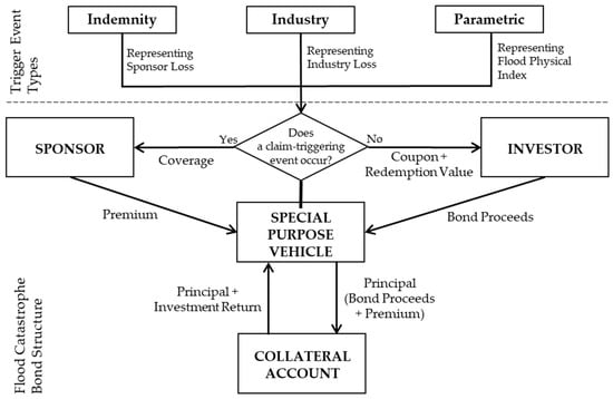
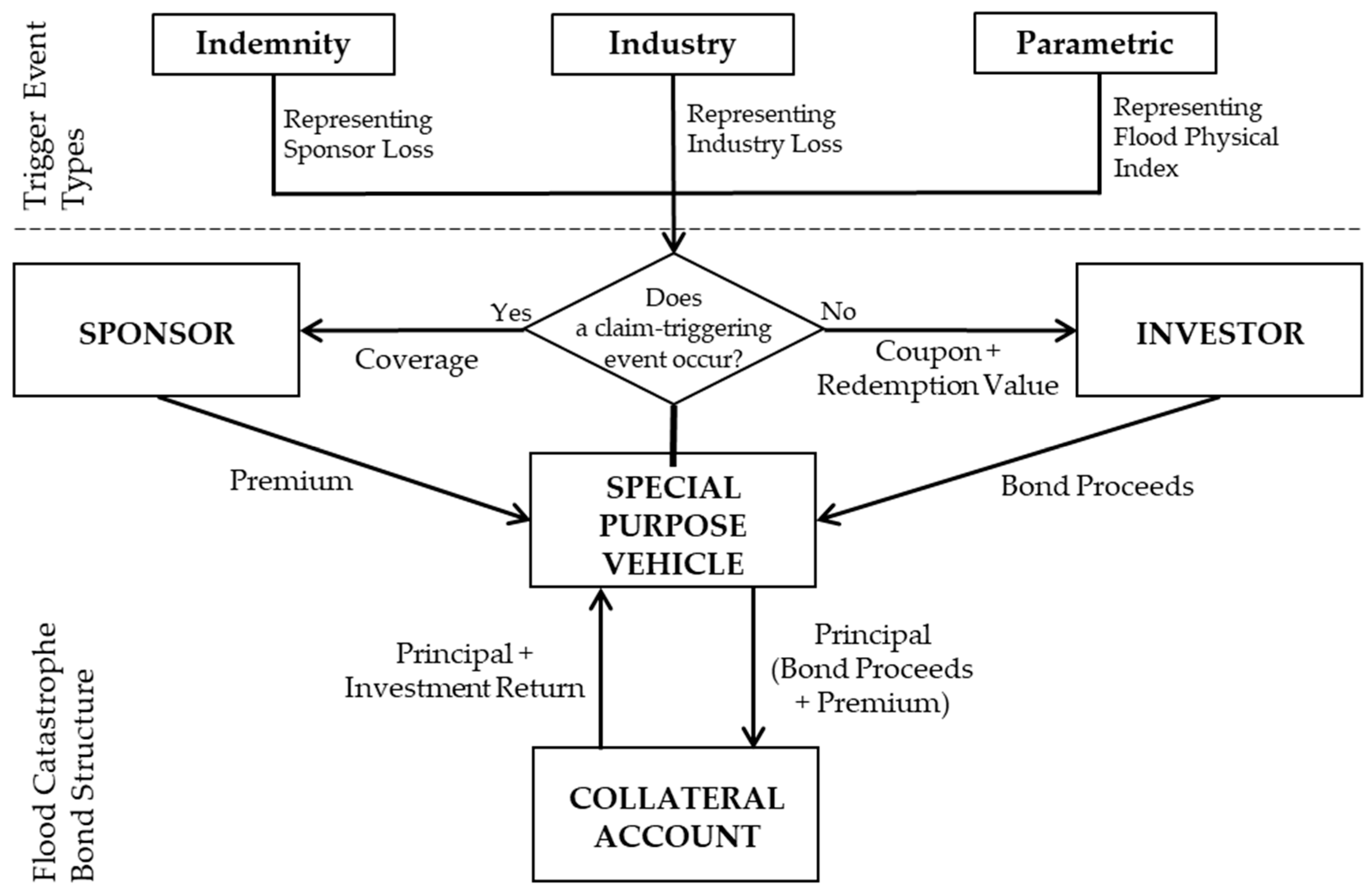
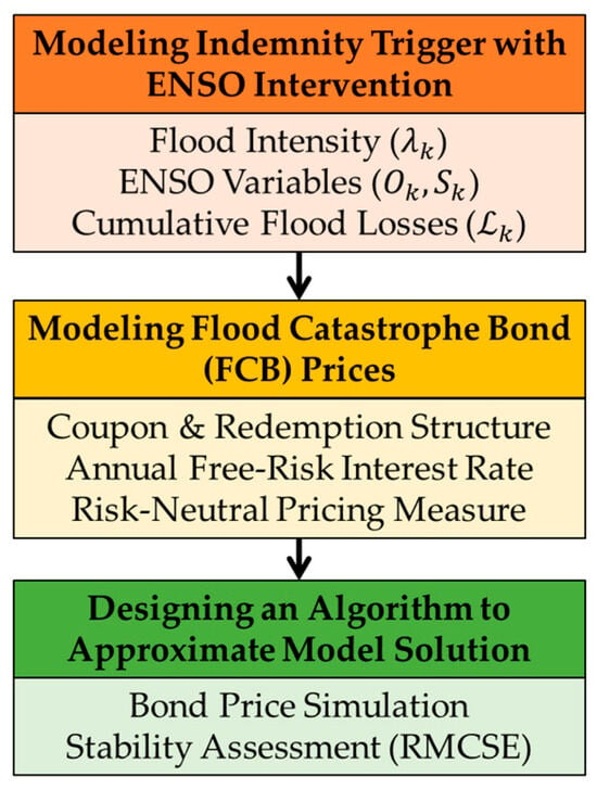
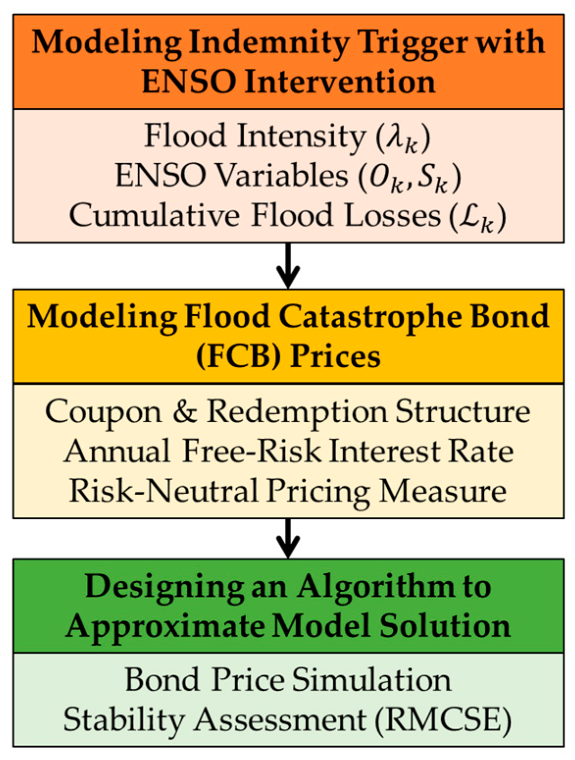
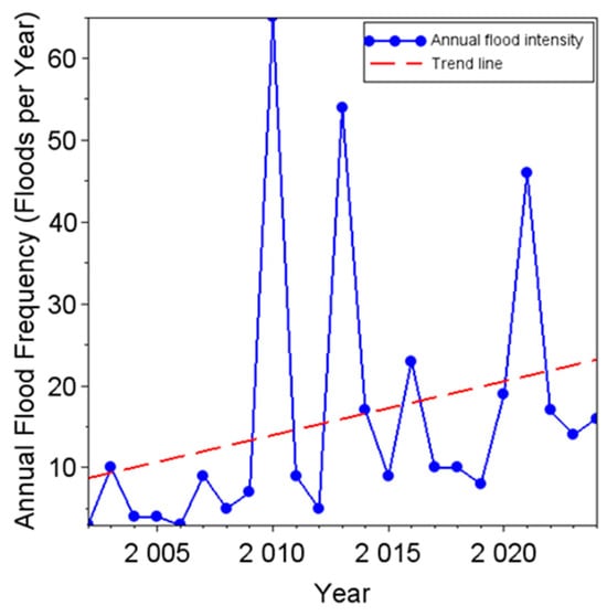
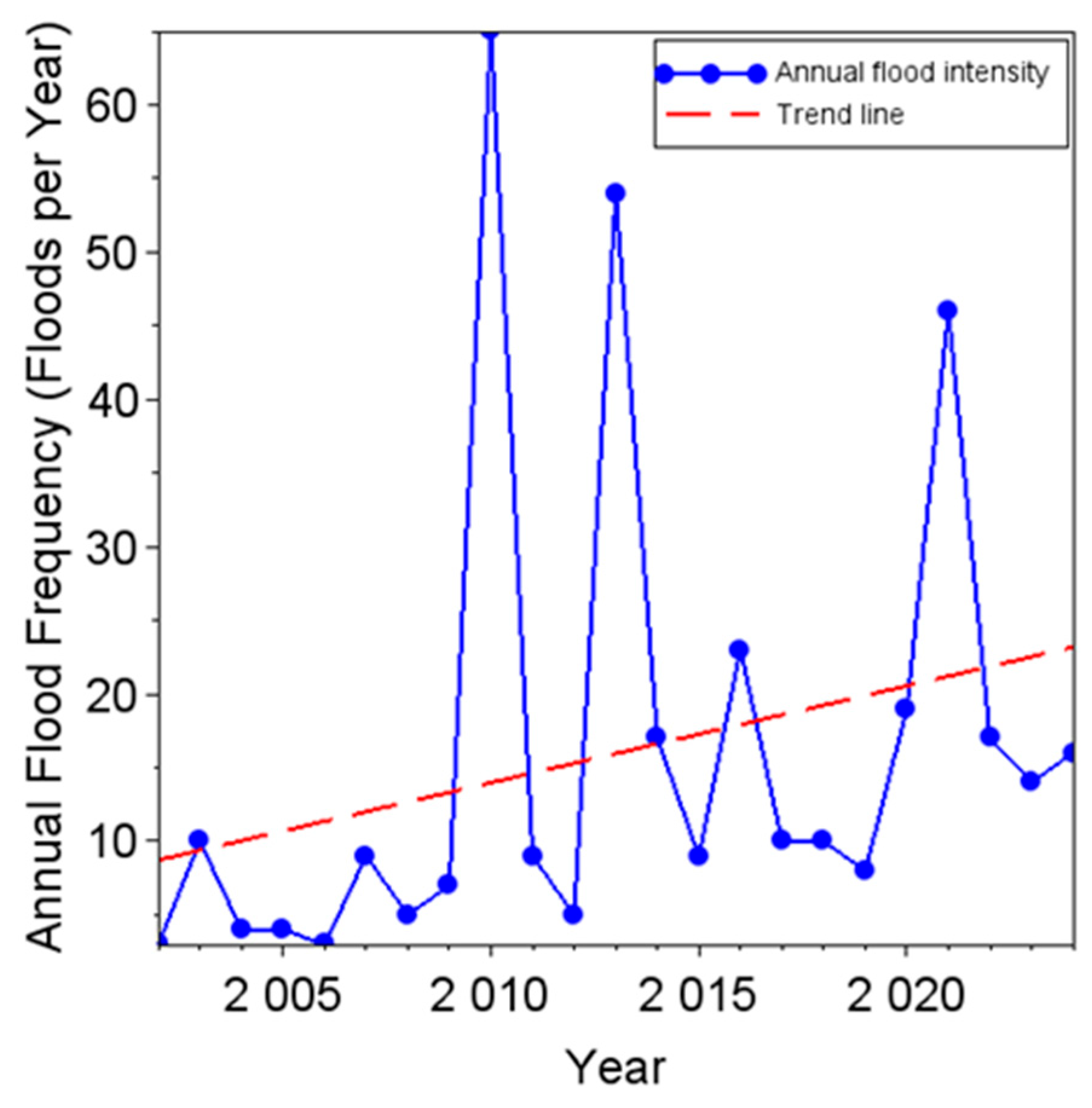
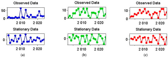
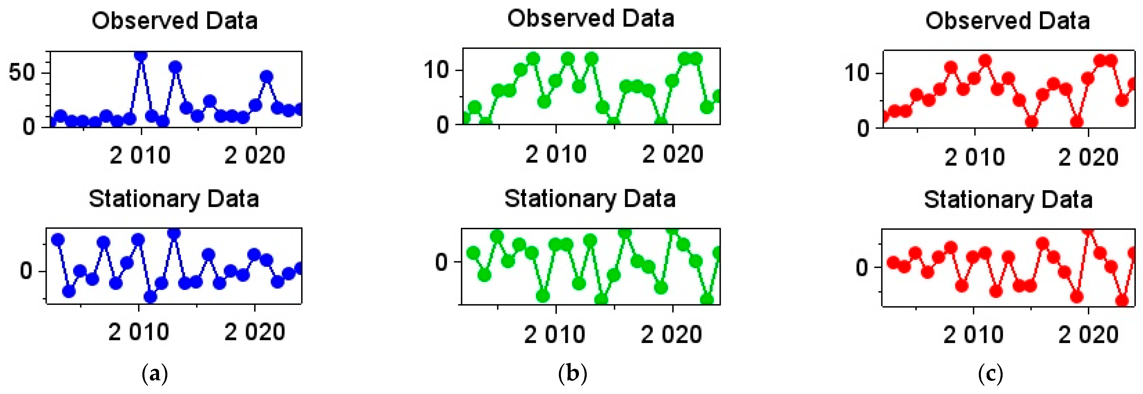
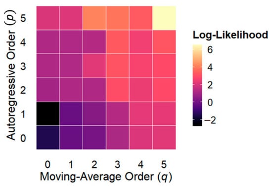
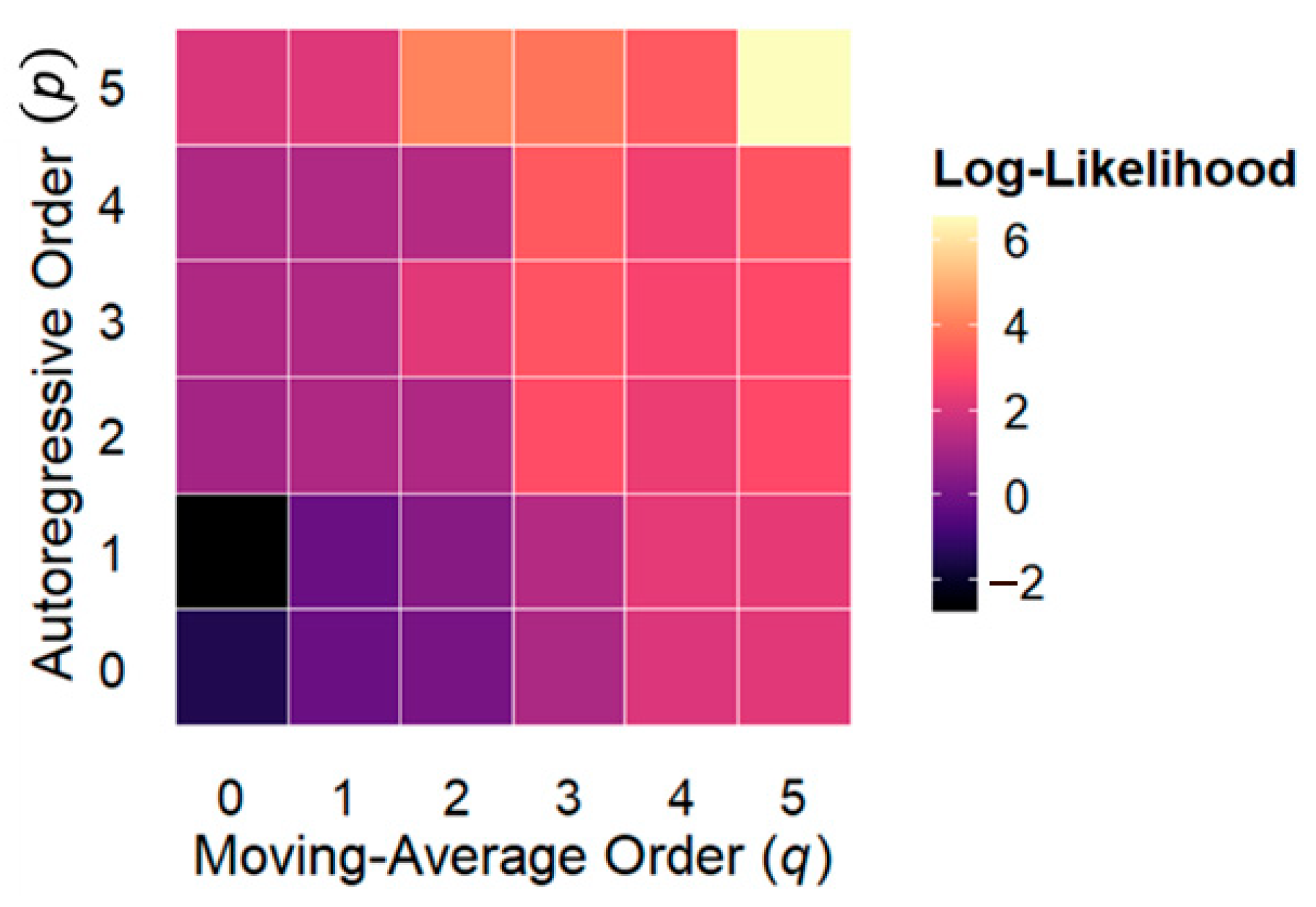
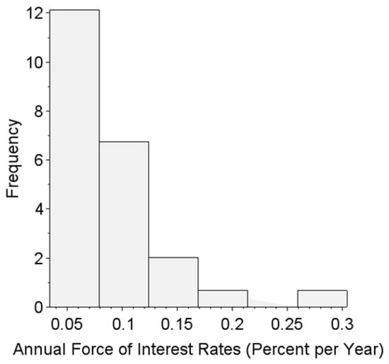
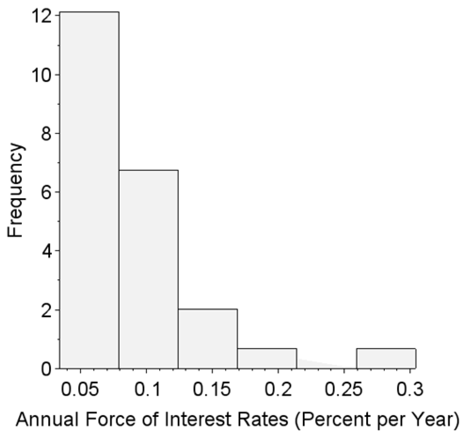
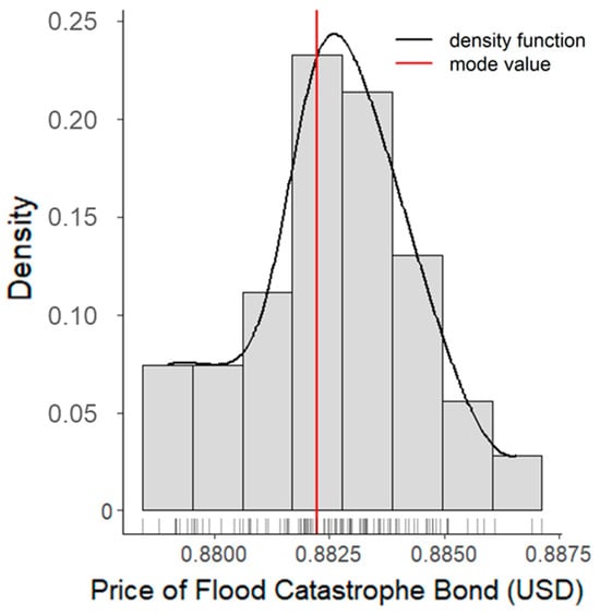
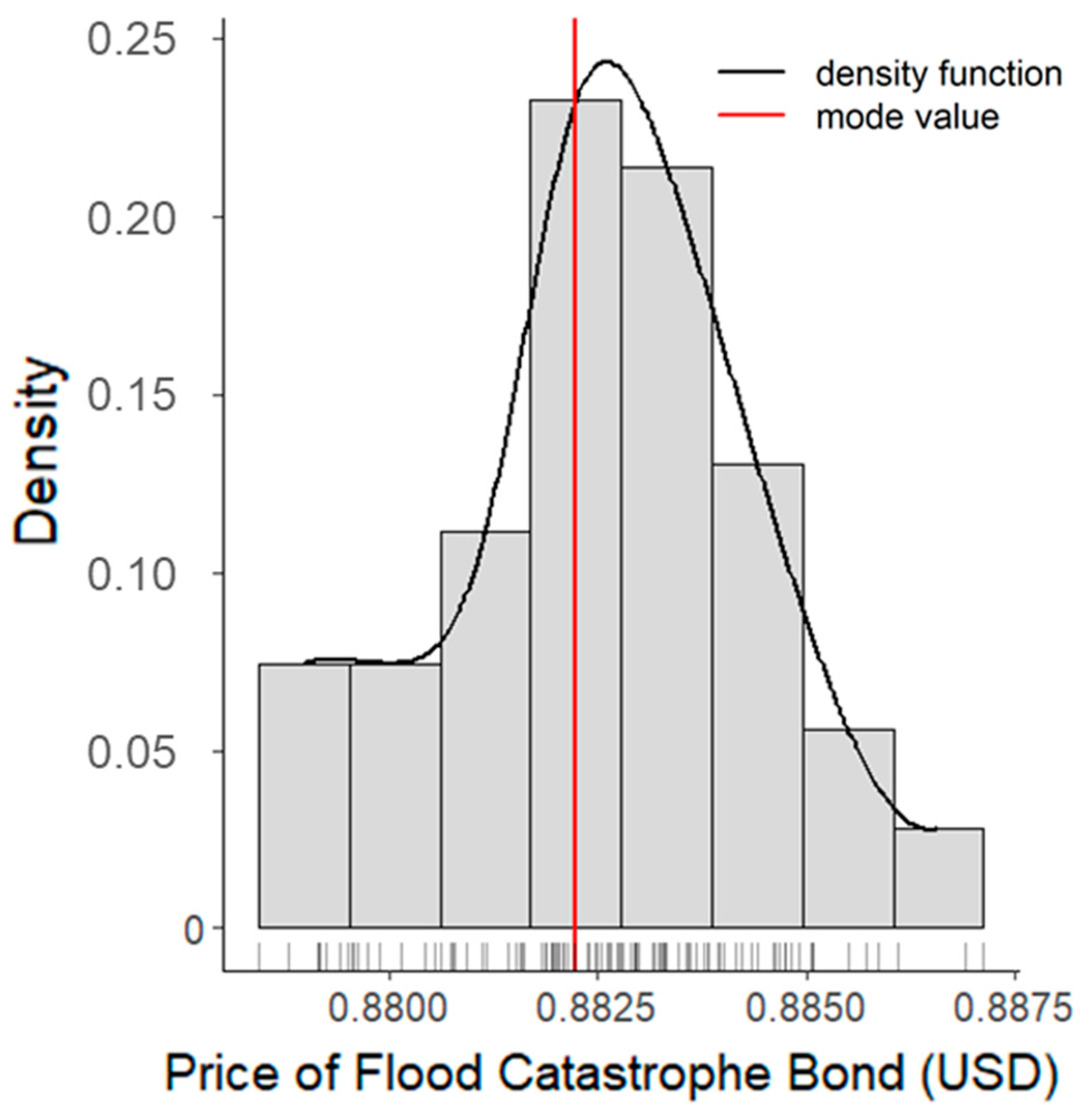

Disclaimer/Publisher’s Note: The statements, opinions and data contained in all publications are solely those of the individual author(s) and contributor(s) and not of MDPI and/or the editor(s). MDPI and/or the editor(s) disclaim responsibility for any injury to people or property resulting from any ideas, methods, instructions or products referred to in the content. |
© 2026 by the authors. Licensee MDPI, Basel, Switzerland. This article is an open access article distributed under the terms and conditions of the Creative Commons Attribution (CC BY) license.