Bivariate Laplace Conditional Distributions for Modeling Non-Linearly Dependent Volatile Price Changes

Abstract

In the spirit of the solution of for modeling price changes in high-volatility markets for univariate commodities, here we generalize an approach to the case of modeling price changes jointly for two related commodities. Often, conditional distributions are more easily understood in financial markets, where the fluctuations in one commodity can shed significant light on the behavior of a related commodity. With this observation, we enhance and characterize the entire family of bivariate joint densities for which both the conditional distributions are specified to be of the Laplace form. Such bivariate distributions will be referred to as bivariate Laplace conditional (BLC) distributions. We study the marginals of the BLC distributions and establish that they are not only sub-Gaussian but also super-Laplacian and, hence, super-Cauchy, i.e., they have heavier tails than Gaussian distributions but lighter tails than the usual Laplace and Cauchy distributions. Distance correlation is suggested as a measure of the association between the two marginal variables, as their product moment correlation is zero but they may be non-linearly dependent. A real-life data set is analyzed to illustrate the use of BCL distributions in practice. We believe that this is the first work using conditional specifications in bivariate financial data analysis.

1. Introduction

It is with deep respect and profound appreciation that we, the authors, dedicate this paper to the memory of the stalwart Professors Joe Gani and Chris Heyde. The first author fondly recalls the wonderful time he spent with Prof. Gani when he was a visiting faculty member at the University of California, Santa Barbara (UCSB), USA, and later also in Australia. It is a pleasure to share here two photos of Prof. Gani. One photo (Figure 1) is with his wife and Prof. S.T. (Zari) Rachev, one of the Editors of this volume, and the other (Figure 2), which reflects the kind and humorous nature of his otherwise serious personality, were taken while all three of them were at UCSB. Prof. Gani has always been an inspiring personality in research and a warm-hearted, cheerful friend.

Figure 1. Joe with Zari in Ashis’s apartment at UCSB in early 1990s.

Figure 2. Joe in a humorous mood in Ashis’s apartment at UCSB in early 1990s.

Rachev and SenGupta (1993) introduced Linnik, or geometric stable, families of distributions to model price change for a single commodity in high-volatility markets. In this paper, we generalize this approach to the case of modeling price changes jointly for two related (bivariate) commodities. Often, conditional distributions are more easily understood in financial markets where the fluctuations in one commodity can shed significant light on the behavior of a related commodity. In Section 2, we briefly introduce the usual Laplace distribution. In Section 3 we enhance and characterize the entire family of bivariate densities for which both the conditional distributions are specified as Laplace distributions, i.e., the family of bivariate conditionally specified Laplace or simply bivariate Laplace conditional (BLC) distributions. Section 4 generalizes the BLC distributions of Section 3 by introducing location parameters. We study in Section 5 the marginals of the BLC distribution and establish that these are not only sub-Gaussian but also super-Laplacian, i.e., they have lighter tails than the usual Laplace distribution and, hence, than the Gaussian distribution. So the BLC distribution is defined in terms of its tail behavior between the Gaussian and Cauchy distributions in the family of $\alpha$-stable distributions, with $1\le \alpha \le 2,$ though it is neither a member of the $\alpha$-stable nor of the Linnik family of distributions. The appealing property of the BLC distribution is that it can be represented in an elegant and analytical closed form in terms of its probability density function (p.d.f.). This property is not available for any distribution, save for merely three (Gaussian, Cauchy and Levy for $\alpha$ = 2, 1 and 0.5 respectively) in the $\alpha$-stable family, and one (Laplace for $\alpha$ = 2) in the Linnik family. Section 6 presents further properties of the BLC and its marginal distributions. Section 7 recalls distance correlation as a useful measure of dependency when the two variables have zero linear correlation but are dependent, as is the case with the variables with the BLC distribution. The statistical inference procedures for the parameters are discussed in Section 8, and the CAN property of the maximum likelihood estimator is established. Section 9 illustrates our proposed model and the corresponding data analysis for a real-life data set on platinum and gold price changes. This example also serves to establish its superiority over the standard bivariate normal model. The closing remarks and conclusions are given in Section 10.

2. Univariate Laplace Models

The classical Laplace distribution is one with a density of the form

$$f(x;\lambda )=(\lambda /2)e^{-\lambda \left|x\right|}I(-\infty <x<\infty ),$$

(1)

where $\lambda$ is a positive intensity parameter.

In the quest for generalizations of the classical central limit theorem and of the family of heavy-tail distributions, Linnik (1963) presented a family of distributions which has been named after him as the family of Linnik distributions. This family essentially consists of symmetric distributions and is obtained through geometric compounding of the stable family of distributions, and hence, is often called the geometric stable family (see, e.g., Rachev & SenGupta, 1993). It has been shown by SenGupta and Roy (2023) that the Linnik family may be viewed as a complementary family to the stable family in terms of its tail behavior. The central role in this family is played by the Laplace distribution, as is done by the Gaussian (normal) distribution for the stable family. There have also been several generalizations of the Laplace distribution on non-Euclidean manifolds (see, e.g., Arnold & SenGupta, 2025).

A well-known property of a symmetric Laplace variable is that it can be represented as a sum or as a 1/2:1/2 mixture of a positive exponential variable and a negative exponential variable. Thus we can write the Laplace variable X in the following two forms in terms of two independent identically distributed exponential $\left(\lambda \right)$ random variables, $V_1$ and $V_2$:

$$X=V_1-V_2,$$

(2)

and

$$X=\left\{\begin{array}{ccc}{V}_1& \mathrm{with}\mathrm{probability}\hfill & 1/2\hfill \\ -V_2& \mathrm{with}\mathrm{probability}\hfill & 1/2.\hfill \end{array}\right.$$

(3)

3. Distributions with Laplace Conditionals

We are interested in absolutely continuous bivariate distributions that have, for each $y\in \mathcal{R}$, a conditional density of X given $Y=y$ of the Laplace form, and for each $x\in \mathcal{R}$, a conditional density of Y given $X=x$ also of the Laplace form.

Thus there will exist two functions $\gamma \left(y\right),\delta \left(x\right)$ such that for $(x,y)\in \mathcal{R}\times \mathcal{R}$, we have

$$\begin{array}{ccc}\hfill f_{X|Y}\left(x\right|y)& =& [\gamma \left(y\right)/2]e^{-\gamma \left(y\right)\left|x\right|},\hfill \end{array}$$

(4)

$$\begin{array}{ccc}\hfill f_{Y|X}\left(y\right|x)& =& [\delta \left(x\right)/2]e^{-\delta \left(x\right)\left|y\right|}.\hfill \end{array}$$

(5)

Denote the density of X as $f\left(x\right)$ and the density of Y as $g\left(y\right)$.

Now for any $(x,y)\in \mathcal{R}\times \mathcal{R}$ the joint density of $(X,Y)$ can be written in two equivalent ways in terms of marginal and conditional densities. We thus will have

$$[\gamma \left(y\right)/2]e^{-\gamma \left(y\right)\left|x\right|}g\left(y\right)=[\delta \left(x\right)/2]e^{-\delta \left(x\right)\left|y\right|}f\left(x\right).$$

(6)

Define $\tau \left(y\right)=log\left[g\right(y\left)\gamma \right(y)/2]$ and $\psi \left(x\right)=log\left[f\right(x\left)\delta \right(x\left)\right]$, and we may rewrite this in the form

$$\tau \left(y\right)-\gamma \left(y\right)\left|x\right|={\psi }_1\left(x\right)-\delta \left(x\right)\left|y\right|$$

(7)

Here $\tau ,\gamma ,\psi$ and $\delta$ are unknown functions. This is a simple functional equation of the Stephanos–Levi Civita–Suto form (see for example, Arnold et al. (1999, p. 13)). The solution is of the form

$$\begin{array}{ccc}\hfill \left(\begin{array}{c}\tau \left(y\right)\\ \gamma \left(y\right)\end{array}\right)& =& A\left(\begin{array}{c}1\\ -\left|y\right|\end{array}\right)\hfill \end{array}$$

(8)

$$\begin{array}{ccc}\hfill \left(\begin{array}{c}\psi \left(x\right)\\ \delta \left(x\right)\end{array}\right)& =& A^{-1}\left(\begin{array}{c}1\\ -\left|x\right|\end{array}\right)\hfill \end{array}$$

(9)

where

$$A=\left(\begin{array}{cc}{a}_{00}& a_{01}\\ a_{10}& a_{11}\end{array}\right).$$

(10)

Upon substituting this solution into the expression for the density on $\mathcal{R}\times \mathcal{R}$ we obtain the following:

Theorem 1.

The family of all bivariate densities which possess Laplace conditionals (BLCs) is of the form

$$\begin{array}{ccc}\hfill f_{X,Y}(x,y)& =& \exp \left[\right(1,-\left|x\right|\left)A\right(1,-{\left|y\right|)}^{\prime }]\hfill \\ & =& \exp [a_{00}-a_{01}|y|-a_{10}|x|+a_{11}|x\left|\right|y\left|\right],\hfill \end{array}$$

(11)

where $-a_{11}<a_{01}.a_{10},a_{01}>0,a_{10}>0,$ and $a_{00}$ is chosen such that

$${\int }_{-\infty }^{\infty }{\int }_{-\infty }^{\infty }\exp \left[\right(1,-\left|x\right|\left)A\right(1,-{\left|y\right|)}^{\prime }]dxdy=1.$$

A perhaps more useful version of this density which is amenable to statistical inference is as follows:

$$f_{X,Y}(x,y)=\kappa (\alpha ,\beta ,\gamma )\exp [-|x|/\alpha -|y|/\beta -(\gamma /\alpha .\beta \left)\right|x\left|\right|y\left|\right].$$

(12)

The parameters $\alpha ,\beta >0,$ can be viewed as scale parameters, while $\gamma$ is a dependency parameter, since X and Y are independent iff $\gamma$ = 0.

Remark 1.

We note that a bivariate Laplace distribution is available from the characteristic function for the multivariate case as given by Anderson (1992).

4. Introducing Location Parameters

There is no problem associated with a simple shift in location in the Laplace conditional density (11) to arrive at the density

$$\begin{array}{ccc}\hfill f_{X,Y}(x,y)& =& \exp {\left[\right(1,-|x-\mu |\left)A\right(1,-|y-\nu |)}^{\prime }]\hfill \\ & =& \exp [a_{00}-a_{01}|y-\nu |-a_{10}|x-\mu |+a_{11}|x-\mu \left|\right|y-\nu \left|\right],\hfill \end{array}$$

(13)

where $a_{11}\le 0,a_{01}>0,a_{10}>0,$ and $a_{00}$ is chosen such that

$${\int }_{-\infty }^{\infty }{\int }_{-\infty }^{\infty }\exp {\left[\right(1,-|x-\mu |\left)A\right(1,-|y-\nu |)}^{\prime }]dxdy=1.$$

A more interesting problem will involve “conditional location shifts”. To resolve this we will need to identify all bivariate densities on $\mathcal{R}\times \mathcal{R}$ such that the conditional densities will be of the form

$$\begin{array}{ccc}\hfill f_{X|Y}\left(x\right|y)& =& [\gamma \left(y\right)/2]e^{-\gamma \left(y\right)|x-\mu (y\left)\right|},\hfill \end{array}$$

(14)

$$\begin{array}{ccc}\hfill f_{Y|X}\left(y\right|x)& =& [\delta \left(x\right)/2]e^{-\delta \left(x\right)|y-\nu (x\left)\right|}.\hfill \end{array}$$

(15)

where $\gamma \left(y\right)$ and $\delta \left(x\right)$ are positive real-valued functions and $\mu \left(y\right)$ and $\nu \left(x\right)$ are real-valued functions.

It appears that our old standby, the Stephanos–Levi Civita–Suto functional equation, will not help us here. This appears to be an intriguing open problem. Intuitively, unless the functions $\mu \left(y\right)$ and $\nu \left(x\right)$ are related (perhaps one is the inverse of the other), it is not obvious that these conditional densities will be compatible.

Henceforth, we will consider the bivariate Laplace conditional (BLC) distributions as members of the family of all possible bivariate distributions whose conditional distributions are Laplace. Thus, it is characterized by the following probability density function:

$$\begin{array}{cc}\hfill f(x,y)& =K\left(\underline{m}\right)\exp \{-(m_{01}\left|x\right|+m_{10}\left|y\right|+m_{11}\left|x\right|\left|y\right|\left)\right\},-\infty <x,y<\infty \hfill \end{array}$$

(16)

where $\underline{m}=(m_{01},m_{10},m_{11})$ and $K\left(\underline{m}\right)$ is the normalizing constant.

Note that here we have slightly changed the notations for the parameters from those of (11) in the previous section. For $f(x,y)$ to exist, the necessary and sufficient condition is $m_{01}>0,m_{10}>0,-m_{11}<m_{01}.m_{10}.$ Observe that when the first two conditions are satisfied, the third condition is trivially satisfied (as a sufficient condition) if $m_{11}\ge 0.$

5. Comparison of the Marginal Distributions with the Standard Laplace Distribution

The marginal distributions can be obtained from the bivariate distribution as given above in (16). The p.d.f of the marginal distribution of X is obtained as follows:

$$\begin{array}{cc}\hfill g\left(x\right)& =C\left(\underline{m}\right){\displaystyle \frac{\exp \{-m_{01}|x\left|\right\}}{m_{10}+m_{11}\left|x\right|}},-\infty <x<\infty \hfill \end{array}$$

(17)

where $C\left(\underline{m}\right)$ is the normalizing constant of $g\left(x\right)$.

Taking $m_{01}=m_{11}=\eta$ (say) in (17) and using the transformation $t=\eta x$, the p.d.f. of t is obtained as

$$\begin{array}{cc}\hfill h\left(t\right)& =D\left(m_{10}\right){\displaystyle \frac{\exp \{-|t\left|\right\}}{m_{10}+\left|t\right|}},-\infty <t<\infty ,\hfill \end{array}$$

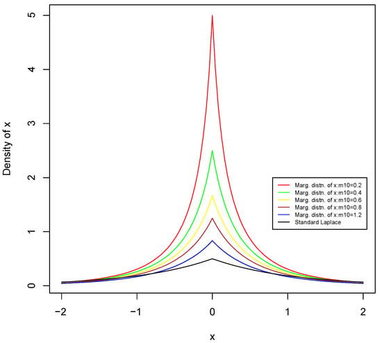
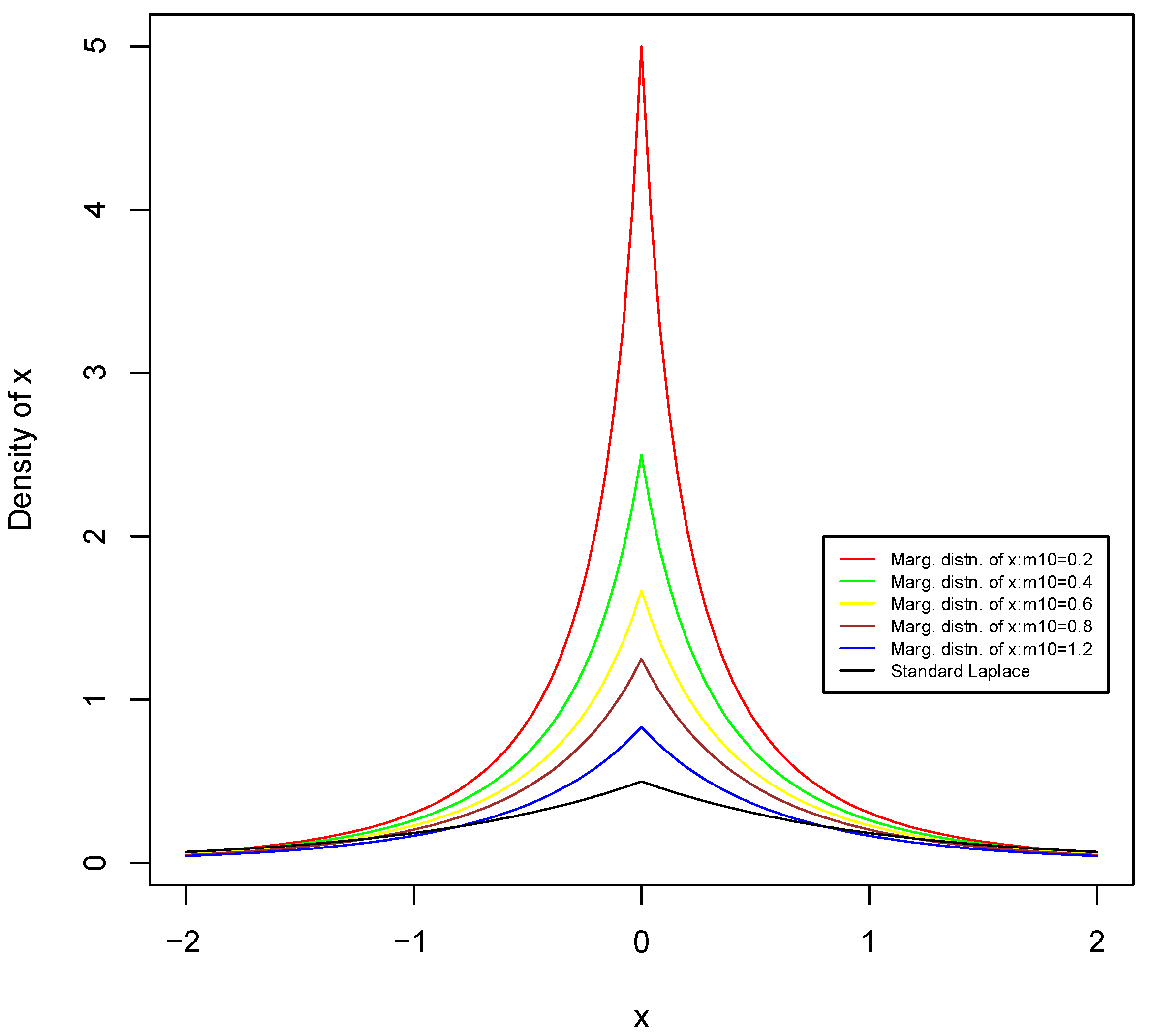
where $D\left(m_{10}\right)$ is the normalizing constant of $h\left(t\right)$. Thus, the scale parameter of the marginal distribution of x is ${\displaystyle \frac{1}{\eta }}$. Now letting $\eta =1$ and taking different values of $m_{10}<1$ (say, $0.2,0.4,0.6$ and $0.8$), we plot the graphs of $h\left(t\right)$ and superimpose them onto that of the standard Laplace density as shown in Figure 3. It is clear that the latter has heavier tails than the former.

Figure 3. Overlay of standard Laplace over BLC marginal distributions.

The different upper ($0.05,0.1,0.01,0.001$ and $0.00001$) percentile points of the standard Laplace distribution are obtained using the VGAM 1.1-14 package in R for Laplace distribution. The computation for a BLC marginal is more involved. Taking the different values of $m_{10}<1$, numerical integration of the p.d.f $h\left(t\right)$ is conducted using the cubature package in R. We set the lower limit to 0 and the upper limit to the corresponding percentile point of the standard Laplace distribution initially. This upper limit is then increased or decreased iteratively by such an amount as to obtain the required coverage probability. The percentile points of the marginals of the bivariate Laplace conditional distributions with different values of $m_{10}<1$ and those of the standard Laplace distribution are presented in Table 1. Again, it is clear that the latter has heavier tails than the former.

Table 1. Comparison of percentile points of the marginal distribution and the standard Laplace distribution.

Upper Percentile	Standard Laplace	Marginal Distribution $\mathit{l}\left(\mathit{t}\right)$
		${\mathit{m}}_{10}=0.2$	${\mathit{m}}_{10}=0.4$	${\mathit{m}}_{10}=0.6$	${\mathit{m}}_{10}=0.8$	${\mathit{m}}_{10}=1.2$
0.1	1.609438	0.1054379	0.2234379	0.3604379	0.5224379	0.9894379
0.05	2.302585	0.1215851	0.2640851	0.4337851	0.6465851	1.372585
0.01	3.912023	0.137023	0.300023	0.502023	0.769023	1.949023
0.001	6.214608	0.1403081	0.3084081	0.5146088	0.794608	2.178208
0.00001	10.81978	0.1406783	0.3087783	0.5198783	0.8027783	2.207878

6. Further Properties of the BLC and Its Marginal Distributions

We now consider some useful and elegant properties of the BLC distribution.

• Observe that $E\left(XY\right)=E\left(X\right)=E\left(Y\right)=0,$ by virtue of symmetry. Thus the BLC distribution models the distribution of two uncorrelated, i.e., linearly independent, but possibly otherwise dependent random variables. Such a situation arises as with high-frequency data, where simple linear dependency within a small time frame may not be apparent, but dependency may exist in a more subtle manner.
• The BLC distribution does also include the case of independence, i.e., when $m_{11}=0.$
• The BLC distribution is a member of the three-parameter regular exponential family (REF). This property is specially useful in developing optimal inference procedures for its parameters, as will be seen below.
• Explicit expressions for $K\left(\underline{m}\right)$ and Var$\left(X\right)$ can be obtained in terms of the classical exponential integral function but are inconsequential for this paper.
• The BLC distribution has Laplace marginals under independence, but not otherwise.

We now present some interesting and useful properties of the marginals of the BLC distribution.

It is well known that the family of $\alpha$-stable distributions does not admit any distribution with an analytical, closed-form p.d.f. for $1<\alpha <2,$ the two extreme values corresponding to the Cauchy and Gaussian distributions respectively. Similarly, the family of Linnik distributions also does not admit any distribution with an analytical, closed form p.d.f. for $1<\alpha <2,$ the upper extreme value corresponding to the Laplace distribution. (Note that $\alpha ,$ the index parameter, is not the same for the two families and its value thus does not quantitatively convey the same properties in the two families.)

• The previous section shows that the following tail ordering, in terms of their rate of decay, holds:

  Gauss (normal) ≺ BCL marginal ≺ Laplace ≺ Cauchy,

  where “≺” represents “lighter tails than”.
• In the family of $\alpha$-stable distributions with $0\le \alpha \le 2,$ the sub-interval $1\le \alpha \le 2,$ has achieved widespread popularity and received special attention, especially for modeling heavy-tail distributions for financial data. Note that the two extremes of this support, $\alpha$ = 1 and 2, correspond to the Gaussian and Cauchy distributions, respectively. However, there is no other distribution known to possess an analytical closed-form representation for it pdf in this interval, and this has led to difficulties in obtaining related optimal inference procedures. Thus, the search for such a distribution has been a challenging task. From the previous item, observe that a marginal of the BLC distribution in general (excluding the Laplace distribution in the case of independence) is defined in terms of its tail behavior between the Gaussian and Cauchy distributions. But, in general, it is neither a member of the $\alpha$-stable family nor of the Linnik family of distributions. The appealing property of this distribution is that it can be represented in an elegant and analytical closed form in terms of its p.d.f., which is not available for any distribution in either of these two families within the tail ordering mentioned above.
• Marginals of the BLC distribution can capture very high kurtosis. This claim is supported by Figure 3.

7. Distance Correlation

The theoretical distance correlation (Szekely et al., 2007) is defined as the distance between the two random vectors $Xϵ{\Re }^p$ and $Yϵ{\Re }^q$ with finite first-order moments, where p and q are positive integers. It is given by

$$\begin{array}{c}\hfill R^2(X,Y)=\left\{\begin{array}{cc}{\displaystyle \frac{{\nu }^2(X,Y)}{\sqrt{{\nu }^2\left(X\right)}\sqrt{{\nu }^2\left(Y\right)}}},\hfill & {\nu }^2\left(X\right){\nu }^2\left(Y\right)>0\hfill \\ 0,\hfill & {\nu }^2\left(X\right){\nu }^2\left(Y\right)=0\hfill \end{array}\right.\end{array}$$

where $\nu (X,Y)$ is the distance covariance given by

$$\begin{array}{c}\hfill {\nu }^2(X,Y)=\left|\right|f_{X,Y}(t,s)-f_X\left(t\right)f_Y\left(s\right){\left|\right|}^2,\end{array}$$

${\nu }^2\left(X\right)$ is the square of the distance variance given by

$$\begin{array}{c}\hfill {\nu }^2\left(X\right)={\nu }^2(X,X)=\left|\right|f_{X,X}(t,s)-f_X\left(t\right)f_X\left(s\right){\left|\right|}^2,\end{array}$$

$f_{X,Y}(t,s)$ is the joint characteristic function of X and Y, and $f_X\left(t\right)$ and $f_Y\left(s\right)$ are the marginal characteristic functions of X and Y respectively.

The empirical distance correlation $R_n(X,Y)$ based on a sample of n bivariate observations $(X_i,Y_i),i=1,...,n,$ is given by

$$\begin{array}{c}\hfill R_n^2(X,Y)={\displaystyle \frac{V_n^2(X,Y)}{\sqrt{V_n^2\left(X\right)}\sqrt{V_n^2\left(Y\right)}}},\end{array}$$

where $V_n(X,Y)$ is the empirical distance covariance given by

$$\begin{array}{cc}\hfill V_n^2(X,Y)={\displaystyle \frac{1}{n^2}}{\displaystyle \sum _{k=1}^n}{\displaystyle \sum _{l=1}^n}{A}_{kl}{B}_{kl},& \\ \hfill A_{kl}& =a_{kl}-\overline{a_{k.}}-\overline{a_{.l}}+\overline{a_{..}},\hfill \\ \hfill B_{kl}& =b_{kl}-\overline{b_{k.}}-\overline{b_{.l}}+\overline{b_{..}},\hfill \\ \hfill a_{kl}=\left|\right|X_k-X_l{\left|\right|}_p,b_{kl}=\left|\right|Y_k-Y_l{\left|\right|}_q,k,l=1,\dots ,n,& \end{array}$$

and the subscript “.” denotes that the mean is computed for the index that it replaces. Also,

$$\begin{array}{c}\hfill V_n^2\left(X\right)={\displaystyle \frac{1}{n^2}}{\displaystyle \sum _{k=1}^n}{\displaystyle \sum _{l=1}^n}{A}_{kl}^2\end{array}$$

8. Statistical Inference for the Parameters of the BLC Distribution

We consider now the method of obtaining the maximum likelihood estimator (MLE) of $\underline{m}.$ The likelihood function of $\underline{m}$ based on a random sample of size n is given by

$$\begin{array}{c}\hfill L\left(\underline{m}\right)={\displaystyle \prod _{i=1}^n}K\left(\underline{m}\right)\exp \{-(m_{01}{\displaystyle \sum _{i=1}^n}\left|x_i\right|+m_{10}{\displaystyle \sum _{i=1}^n}\left|y_i\right|+m_{11}{\displaystyle \sum _{i=1}^n}\left|x_i\right|\left|y_i\right|\left)\right\}\end{array}$$

The likelihood equations can be written down easily save the part involving $K\left(\underline{m}\right),$ which is represented in terms of a bivariate integral. An iterative method is thus needed to solve these equations, and one can use the ’optim’ function in R.

For the iterative method, the initial values of the parameters $m_{01}$ and $m_{10}$ can be taken as the reciprocals of the standard deviations of $\left|X\right|$ and $\left|Y\right|$ respectively. For $m_{11},$ the initial value can be taken as the absolute value of the correlation between $\left|X\right|$ and $\left|Y\right|$ divided by the product of their two standard deviations.

The efficiency of the MLEs can be measured through the computation of the standard errors of the estimators. The standard errors are obtained from the diagonal elements of the inverse of the Fisher information matrix based on n observations.

The Fisher information matrix, I, is given by

$$\begin{array}{cc}\hfill I\left(\underline{m}\right)& =E\left[\left({\displaystyle \frac{\partial \ln f}{\partial \underline{m}}}\right){\left({\displaystyle \frac{\partial \ln f}{\partial \underline{m}}}\right)}^{\prime }\right]=E\left(\begin{array}{ccc}{a}^2& ab& ac\\ ab& b^2& bc\\ ac& bc& c^2\end{array}\right),\hfill \end{array}$$

where

$$\begin{array}{cc}\hfill a& ={\displaystyle \frac{\partial \ln f}{\partial m_{01}}}=K\left(\underline{m}\right){\int }_{-\infty }^{\infty }{\int }_{-\infty }^{\infty }\left|x\right|\exp \{-m_{01}\left|x\right|-m_{10}\left|y\right|-m_{11}\left|x\right|\left|y\right|\}dxdy-\left|x\right|\hfill \\ \hfill & =E\left[\right|X\left|\right]-\left|X\right|,\hfill \end{array}$$

$$\begin{array}{cc}\hfill b& ={\displaystyle \frac{\partial \ln f}{\partial m_{10}}}=K\left(\underline{m}\right){\int }_{-\infty }^{\infty }{\int }_{-\infty }^{\infty }\left|y\right|\exp \{-m_{01}\left|x\right|-m_{10}\left|y\right|-m_{11}\left|x\right|\left|y\right|\}dxdy-\left|y\right|\hfill \\ \hfill & =E\left[\right|Y\left|\right]-\left|Y\right|,\hfill \end{array}$$

$$\begin{array}{cc}\hfill c& ={\displaystyle \frac{\partial \ln f}{\partial m_{10}}}=K\left(\underline{m}\right){\int }_{-\infty }^{\infty }{\int }_{-\infty }^{\infty }\left|x\right|\left|y\right|\exp \{-m_{01}\left|x\right|-m_{10}\left|y\right|-m_{11}\left|x\right|\left|y\right|\}dxdy-\left|x\right|\left|y\right|\hfill \\ \hfill & =E\left[\right|X\left|\right|Y\left|\right]-\left|X\right|\left|Y\right|.\hfill \end{array}$$

Therefore, we get

• $E\left[a^2\right]=E\left[E^2\left|X\right|\right]+E\left[X^2\right]-2E\left[\left|X\right|E\left|X\right|\right]=Var\left(\right|X\left|\right),$
• $E\left[ab\right]=E\left[E\left|X\right|E\left|Y\right|\right]-E\left[\left|Y\right|E\left|X\right|\right]-E\left[\left|X\right|E\left|Y\right|\right]+E\left[\left|X\right|\left|Y\right|\right]=Cov\left(\right|X|,|Y\left|\right),$
• $E\left[ac\right]=E\left[E\left|X\right|E\left|X\right|\left|Y\right|\right]-E\left[\left|X\right|\left|Y\right|E\left|X\right|\right]-E\left[\left|X\right|E\left|X\right|\left|Y\right|\right]+E\left[X^2\left|Y\right|\right]=Cov\left(\right|X|,|X\left|\right|Y\left|\right),$
• $E\left[b^2\right]=E\left[E^2\left|Y\right|\right]+E\left[Y^2\right]-2E\left[\left|Y\right|E\left|Y\right|\right]=Var\left(\right|Y\left|\right),$
• $E\left[bc\right]=E\left[E\left|Y\right|E\left|X\right|\left|Y\right|\right]-E\left[\left|X\right|\left|Y\right|E\left|Y\right|\right]-E\left[\left|Y\right|E\left|X\right|\left|Y\right|\right]+E\left[Y^2\left|X\right|\right]=Cov\left(\right|Y|,|X\left|\right|Y\left|\right),$
• $E\left[c^2\right]=E\left[E^2\left|X\right|\left|Y\right|\right]+E\left[X^2{Y}^2\right]-2E\left[\left|X\right|\left|Y\right|E\left|X\right|\left|Y\right|\right]=Var\left(\right|X\left|\right|Y\left|\right).$

Remark 2.

The above results, though derived directly, also follow by appealing to the properties of the score functions of a multi-parameter REF.

Since the BLC distribution is a member of the REF, the Cramer regularity conditions required to establish Theorem 2 are satisfied.

Theorem 2.

Let $\widehat{\underline{m}}$ be the maximum likelihood estimator of $\underline{m}.$ Then,

$$\sqrt{n}(\widehat{\underline{m}}-\underline{m})\stackrel{L}{\to }{\mathcal{N}}_3(0,I^{-1})asn\to \infty .$$

The above result provides the consistency and asymptotic normality (CAN) properties of the MLE $\widehat{\underline{m}}$ of $\underline{m}.$ It can also be used to yield asymptotic confidence intervals and consistent tests for $\underline{m}.$

9. Real-Life Example

We now present a real-life data set to illustrate the application of our BLC model. Recall that this model does not apply to situations where the two variables have a non-zero product moment correlation.

The daily price data on diamond and platinum were collected from the internet for the n paired observations for the months from May to July, 2025. Let the prices be denoted by $x_{1t}$ and $x_{2t}$ respectively.

We make the log-ratio transformation on $x_{1t}$ and $x_{2t}$ as follows.

$$y_{1t}=100(\ln \left(x_{1t}\right)-\ln \left(x_{1,t-1}\right))\mathrm{and}{y}_{2t}=100(\ln \left(x_{2t}\right)-\ln \left(x_{2,t-1}\right)).$$

The obtained sample correlation between $y_{1t}$ and $y_{2t}$ is $-0.01066954$.

The obtained sample distance correlation between $y_{1t}$ and $y_{2t}$ is $0.1848587$.

Observe that the linear correlation is very small and negligible. However, the distance correlation has a moderate value. This indicates that while linear dependency does not exist, non-linear dependency might. We thus advocate the use of our BCL model for this data set.

We follow the details given in Section 9 above for obtaining the MLE of $\underline{m}.$ The initial estimates of the parameters $m_{01}$, $m_{10}$ and $m_{11}$ are $8.906111$, $7.550306$ and $49.7322$ respectively. The following MLEs of the parameters are then obtained: $\widehat{m_{01}}=28.13994,\widehat{m_{10}}=7.83915$ and $\widehat{m_{11}}=30.19539$.

The empirical Fisher information matrix based on the n observations is obtained:

$$\begin{array}{cc}\hfill nI\left(\underline{m}\right)& =\left(\begin{array}{ccc}2.642579e-03& -8.934507e-05& 9.175539e-06\\ -8.934507e-05& 2.344128e-04& 2.496011e-05\\ 9.175539e-06& 2.496011e-05& 1.282111e-03\end{array}\right)\hfill \end{array}$$

The corresponding inverse of the Fisher information matrix is obtained:

$$\begin{array}{cc}\hfill {\left(nI\left(\underline{m}\right)\right)}^{-1}& =\left(\begin{array}{ccc}383.39849& 146.72641& -5.60029\\ 146.72641& 4330.99250& -85.36571\\ -5.60029& -85.36571& 781.66553\end{array}\right)\hfill \end{array}$$

The standard errors of the estimators are obtained: $s.e.\left(m_{01}\right)=19.58056$, $s.e.\left(m_{10}\right)=65.81028$ and $s.e.\left(m_{11}\right)=27.95828$. Given the small sample size, the estimators obtained can be considered to be reasonably efficient.

We have already noted that linear correlation is negligible, implying that there is no linear dependency between $Y_1$ and $Y_2$. The BLC model is a reasonable candidate here since it can capture possible non-linear dependency. Theorem 2 provides the necessary test (with large samples) by testing for $H_0:m_{11}=0$ against $H_1:m_{11}\ne 0.$ The critical region is given by:

$$\omega :\left|\widehat{\underline{m}}\right|>[s.e.\left(m_{11}\right)]{\tau }_{\alpha /2},$$

where ${\tau }_{\alpha }$ is the upper $\alpha$-percentile point of the standard normal distribution. Taking $\alpha$ = 0.30, ${\tau }_{0.15}$ is 1.02. Hence, for this example (for a somewhat moderate level of significance), independence between $Y_1$ and $Y_2$ is rejected in favor non-linear dependency.

To demonstrate its usefulness in real-life applications, the performance of the proposed BLC distribution is compared with the bivariate normal distribution for the above data set. We do this through the use of the formal goodness-of-fit metrics viz. the Akaike information criterion (AIC) and Bayesian information criterion (BIC). The Akaike information criterion (AIC) is given by

$$\begin{array}{cc}\hfill AIC& =-2\ln L_{max}+2\times k\hfill \end{array}$$

The Bayesian information criterion (BIC) is given by

$$\begin{array}{cc}\hfill BIC& =-2\ln L_{max}+k\times \ln \left(n\right)\hfill \end{array}$$

where n is the number of observations and k is the number of estimated parameters. In the case of the BLC distribution, $k=3,$ while for the bivariate normal distribution, $k=5$.

The smaller the AIC or BIC value of a distribution, the better the fit of the distribution to the given data.

We now compare the performance of our BLC distribution and the bivariate normal distribution models for this data set. The AIC and BIC values for the data are displayed in Table 2.

Table 2. AIC and BIC values for bivariate normal and BLC distributions.

Distribution	BIC	AIC
Bivariate normal	−891.4517	−905.3892
Bivariate Laplace conditionals	−85,109.22	−85,119.69

It is clear from the above table that the bivariate Laplace conditional distribution gives a better fit to the given data than the bivariate normal distribution.

10. Remarks and Conclusions

This paper was prompted by several facts: 1. There is no distribution with a closed-form p.d.f. in the $\alpha$-stable family in the important region $1<\alpha <2$, i.e., there are no tails in between the normal and Cauchy distributions. 2. Bivariate distributions with marginals as stated in item 1 are not readily available. 3. High-frequency data on a bivariate random variable may exhibit zero linear correlation, but strong dependency can exist. 4. In practice, it is often easier and more meaningful to specify the conditionals of a bivariate distribution. The bivariate Laplace conditional distribution proposed here provides a solution to items 1–3 based on its construction, which is enhanced by item 4. Further, asymptotic optimal inference procedures for the parameters of this model have been readily derived. We believe that this is the first work using conditional specifications in bivariate financial data analysis. It is hoped that the elegant representation of the bivariate p.d.f. for the BLC family of distributions, coupled with its attractive and useful properties for real-life applications, will motivate further research in this new direction.

References

- Anderson, D. N. (1992). A multivariate Linnik distribution. Statistics and Probability Letters, 14, 333–336. [Google Scholar] [CrossRef] [Scilit]
- Arnold, B. C., Castillo, E., & Sarabia, J. M. (1999). Conditional specification of statistical models. Springer. [Google Scholar]
- Arnold, B. C., & SenGupta, A. (2025). Wrapping generalized Laplace and generalized discrete Laplace distributions. Axioms, 14(7), 529. [Google Scholar] [CrossRef] [Scilit]
- Linnik, J. V. (1963). Linear forms and statistical criteria I, II. In Selected transactions in mathematical statistics and probability (Vol. 3, pp. 1–90). American Mathematical Society. [Google Scholar]
- Rachev, S. T., & SenGupta, A. (1993). Laplace—Weibull mixtures for modelling price changes. Management Science, 39, 1029–1038. [Google Scholar] [CrossRef] [Scilit]
- SenGupta, A., & Roy, M. (2023). A characteristic function based circular distribution family and its goodness of fit: The flexible wrapped Linnik family. Journal of Applied Statistics, 51(12), 2364–2381. [Google Scholar] [CrossRef] [Scilit] [PubMed]
- Szekely, G. J., Rizzo, M. L., & Bakirov, N. K. (2007). Measuring and testing dependence by correlation of distances. Annals of Statistics, 35(6), 2769–2794. [Google Scholar] [CrossRef] [Scilit]
Disclaimer/Publisher’s Note: The statements, opinions and data contained in all publications are solely those of the individual author(s) and contributor(s) and not of MDPI and/or the editor(s). MDPI and/or the editor(s) disclaim responsibility for any injury to people or property resulting from any ideas, methods, instructions or products referred to in the content. |
© 2026 by the authors. Licensee MDPI, Basel, Switzerland. This article is an open access article distributed under the terms and conditions of the Creative Commons Attribution (CC BY) license.