


Abstract
Spot Bitcoin exchange-traded funds (ETFs) have renewed the question of whether Bitcoin is “digital gold”. We define digital gold as an asset that is a safe haven in equity declines and can replace gold in a portfolio without raising its tail risk, and test both properties in two equity–bond portfolios that differ only in holding Bitcoin or gold. We use ETF data (607 trading days, 2024–2026) and longer Bitcoin (2014–2026) and gold (2000–2026) series. The Bitcoin portfolio’s 95% Expected Shortfall is 1.63 times that of the gold portfolio in the ETF sample (95% CI 1.36–1.99) and 2.48 times over 2014–2026. The gap reflects volatility: over the long sample, volatility-standardized ES95 is equivalent within the chosen margin. Bitcoin’s dependence on equities in extreme declines is positive in every sample and regime; after adjustment for equity volatility, no contagion is detected, subject to the adjustment’s assumptions. Gold decouples from equities in crises but is not shown to be a weak safe haven. Minimum-variance and minimum-CVaR optimizers give Bitcoin almost no weight. The conclusions concern the historical risk of the instruments and periods studied, not Bitcoin’s fundamental value or unobserved structural risks; crisis, tail-day and 99% estimates rest on few observations.
1. Introduction
Since the publication of the Bitcoin white paper (Nakamoto, 2008), Bitcoin has gradually moved into the spotlight of global investors. In January 2024 the U.S. Securities and Exchange Commission (SEC) approved the first spot Bitcoin ETFs, which gave investors a regulated channel to Bitcoin price exposure (U.S. Securities and Exchange Commission, 2024). The funds attracted more than $75 billion of new assets in their first year (Hornback & Whaley, 2025), and the market quickly became concentrated, with more than half of its assets in a single product (Oefele, 2025). Whether Bitcoin behaves as “digital gold” has therefore become a practical question for portfolio construction, not only a theoretical one.
The evidence is mixed. Gold has been found to be a hedge against equities and a safe haven in extreme market declines (Baur & Lucey, 2010; Baur & McDermott, 2010). Most studies of Bitcoin before the approval of spot ETFs conclude that it is mainly a diversifier rather than a hedge or a safe haven (Bouri et al., 2017; Klein et al., 2018; Shahzad et al., 2020), and it fell together with equities in the COVID-19 crash (Conlon & McGee, 2020). Other studies find safe-haven behavior under specific conditions or against geopolitical risk (Chibane & Janson, 2025; P. Liu & Yuan, 2024). Since the approval, Bitcoin’s correlation with equities has risen (Hong et al., 2025; Lee & Lee, 2025; Wu, 2025).
Two features limit what this literature can say about the question investors now face. First, it measures Bitcoin with exchange prices and rarely asks whether a spot Bitcoin ETF can take gold’s place in the same portfolio. Second, the ETF era is short: a sample that starts in January 2024 covers one market environment, with few days of severe stress. We therefore study two complementary samples with equal weight. The ETF sample (January 2024–June 2026, 607 trading days) uses the funds themselves. The long samples use Bitcoin spot prices from September 2014 (2952 days) and gold prices from August 2000 (6466 days), and cover the global financial crisis, the euro-area crisis, the COVID-19 crash and the inflation and energy shock of 2022.
The question is examined through a controlled portfolio comparison: two portfolios with the same equity and bond ETFs that differ only in whether Bitcoin or gold occupies the same one-third sleeve. It is formalized as four hypotheses with stated decision rules—two asset-level hypotheses on dependence and safe-haven behavior and two portfolio-level hypotheses on tail risk and portfolio substitution—and the hypotheses intended for confirmation are distinguished from exploratory and robustness analyses. Market regimes are identified with a Markov-switching model and a VIX threshold model estimated on the long samples.
The paper makes four contributions. First, it measures how much more tail risk a portfolio carries when Bitcoin rather than gold occupies the same sleeve, decomposes the difference exactly into a volatility term and a standardized ES (tail-shape) term with an equivalence test for the latter, and expresses it as a risk-equivalent Bitcoin weight w*, together with how imprecisely that weight is estimated. That the equally weighted Bitcoin portfolio is the riskier one follows largely from Bitcoin’s volatility; the decomposition and w* are the informative results. Second, it tests safe-haven behavior for Bitcoin and gold with the same rules, including an equivalence test of weak safe-haven status, complemented by regime-dependent regressions and an episode study of every equity drawdown of 10% or more since 2000, and shows what the short ETF sample can and cannot identify.
Third, applying the result of Boyer et al. (1997) and Forbes and Rigobon (2002) that a correlation rises with market volatility even when the underlying relation is unchanged, it separates correlation from sensitivity and interdependence from contagion: Bitcoin’s correlation with equities rises in crisis regimes, but once the higher volatility of equities is taken into account the rise is not significant. Fourth, it separates Bitcoin from the ETF that holds it, splitting IBIT’s risk into a trading-hours effect and a vehicle-and-measurement effect, and asks with spanning tests and out-of-sample optimization whether Bitcoin expands the opportunity set of a portfolio that holds gold, and whether gold expands one that holds Bitcoin. Throughout, the paper reports interval estimates and states where inference is conditional on estimated parameters or adjusted for multiple comparisons.
The remainder of the paper is organized as follows. Section 2 reviews the literature. Section 3 describes the data and their distributional properties, the definitions and hypotheses, and the methods. Section 4 reports the results. Section 5 discusses them around four mechanisms—volatility scaling, the shape of the distribution, dependence in market declines and the role in portfolios—and Section 6 concludes with policy implications, limitations and directions for future research. Appendix A, Appendix B, Appendix C, Appendix D, Appendix E, Appendix F, Appendix G, Appendix H, Appendix I and Appendix J document the data and report the detailed and robustness results.
2. Literature Review
This section reviews seven strands of research on which the paper builds: the hedge and safe-haven properties of gold (Section 2.1); the corresponding evidence for Bitcoin (Section 2.2); the early evidence on spot Bitcoin ETFs (Section 2.3); the efficiency and connectedness of cryptocurrency markets (Section 2.4); the measurement, forecasting and backtesting of tail risk (Section 2.5); portfolio choice under estimation error (Section 2.6); and regime dependence and contagion (Section 2.7). Section 2.8 identifies the gaps that the paper addresses.
2.1. Gold as a Hedge and Safe Haven
Baur and Lucey (2010) introduced the distinction, adopted in this paper, between a hedge, a diversifier and a safe haven. Using U.S., U.K. and German data, they find that gold is a hedge against stocks on average and a safe haven in extreme stock market conditions, but that the safe-haven property is short-lived. Baur and McDermott (2010) extend the analysis to international data for 1979–2009 and distinguish weak from strong safe havens: gold is both a hedge and a safe haven for the major European stock markets and the United States, but not for Australia, Canada, Japan and large emerging markets, and it acted as a strong safe haven for most developed markets at the peak of the 2008 financial crisis. Reboredo (2013) uses copulas to show that gold is also a hedge against depreciation of the U.S. dollar and an effective safe haven against its extreme movements.
Later studies qualify these conclusions along three dimensions. The first is the market: in smooth-transition regressions for 18 national markets and five regional indices over 1970–2012, Beckmann et al. (2015) confirm that gold serves as both a hedge and a safe haven but find that this ability is market-specific. The second is the state of the market: Hood and Malik (2013) find that gold is a hedge and a weak safe haven for the U.S. stock market, but that its correlation with stocks is not negative in periods of extremely low or high volatility, and that the VIX offers better protection. The third is the horizon: using wavelet methods, Bredin et al. (2015) show that gold is a hedge for a range of international equity and debt markets at horizons of up to one year and a safe haven for equities during crises, with the exception of the early-1980s recession. Gold’s protective role also has limits beyond equity markets: Erb and Harvey (2013) show that gold is an unreliable inflation hedge over practical investment horizons and that high real gold prices have historically been followed by below-average returns.
Two lessons from this literature shape our design. The safe-haven property is defined by an asset’s dependence on equities in extreme declines, so any test of it rests on the few observations in the tail; and the evidence for gold is itself conditional on the market, the volatility regime and the horizon. Gold is therefore treated here as a benchmark to be measured over the same sample as Bitcoin, and its safe-haven property is tested (H2b) rather than assumed.
2.2. Bitcoin as a Hedge, Diversifier or Safe Haven
Early studies approached Bitcoin through the lens of the gold literature. Estimating GARCH models, Dyhrberg (2016) finds several similarities between Bitcoin, gold and the U.S. dollar that indicate hedging capabilities, and places Bitcoin between gold and the dollar; a replication and extension of that study, however, finds Bitcoin’s returns, volatility and correlations distinct from those of both gold and the dollar (Baur et al., 2018a). Brière et al. (2015), using weekly data for 2010–2013, report very high average returns and volatility, very low correlations with other assets and significant diversification benefits even from small allocations, while cautioning that these may reflect an early stage of the market. Studies that applied the framework of Baur and Lucey (2010) directly were less favorable. Bouri et al. (2017) conclude that Bitcoin is a poor hedge and suitable for diversification purposes only, with strong safe-haven behavior limited to weekly extreme declines in Asian stocks. Klein et al. (2018) find that Bitcoin is positively correlated with falling markets, shows no stable hedging capability and shares none of gold’s distinctive properties other than an asymmetric response of its volatility. Baur et al. (2018b) document that Bitcoin was uncorrelated with traditional asset classes in both normal and turbulent periods and was held mainly as a speculative investment rather than used as a medium of exchange.
Comparing the two assets for the G7 stock markets, Shahzad et al. (2020) find that gold is a safe haven and hedge for several of the indices, whereas Bitcoin plays these roles only for Canada, and that gold’s hedging and diversification benefits are larger and more stable. Smales (2019) argues that, because Bitcoin is more volatile, less liquid and costlier to trade than gold, it is unlikely to be worth considering as a safe haven until its market matures. The answer also depends on the asset to be protected: using hourly data, Urquhart and Zhang (2019) find that Bitcoin is an intraday hedge for some currencies, a diversifier for others and a safe haven for the Canadian dollar, the Swiss franc and the British pound during extreme market turmoil.
The market crash of March 2020 provided a natural test. Conlon and McGee (2020) find that Bitcoin did not act as a safe haven, falling in lockstep with the S&P 500, and that even a small allocation to Bitcoin substantially increased portfolio downside risk. Corbet et al. (2020) show that the volatility relationship between the main Chinese stock markets and Bitcoin changed significantly during that period of extreme financial stress. Using a vector autoregression, Choi and Shin (2022) find that Bitcoin prices rise after inflation shocks but, unlike gold, fall in response to financial uncertainty shocks, which rejects the safe-haven property.
More recent studies report safe-haven behavior under specific conditions. Using time-varying-parameter connectedness measures around the COVID-19 period, P. Liu and Yuan (2024) find that including Bitcoin reduces total connectedness with currency, bond and stock markets and that Bitcoin offers hedging and safe-haven capabilities during turbulence. Chibane and Janson (2025) find that Bitcoin and the Swiss franc act as safe havens against geopolitical risk, mainly during large market moves, whereas gold and Treasury bonds do not. Sodnomdavaa (2026) finds that causality between Bitcoin and gold over 2013–2025 is generally weak and that gold’s influence on Bitcoin strengthens only in stress periods and at longer horizons.
Three features of the literature matter for our design. First, conclusions differ with the sample period, the data frequency, the reference market and the method, and much of the favorable evidence is conditional on particular episodes or conditions, so results obtained before 2024 need not describe the ETF era. Second, because spot ETFs did not exist before 2024, these studies use Bitcoin prices from cryptocurrency exchanges or data aggregators, which trade around the clock and are commonly recorded at midnight UTC, whereas equity benchmarks close at 16:00 ET; such asynchronous prices understate measured daily co-movement, much as nonsynchronous trading biases estimated betas (Scholes & Williams, 1977), an issue we address in Section 3.10. Third, the safe-haven property is a statement about a few extreme days, so a failure to reject a zero or negative tail slope may reflect low power rather than a safe haven. We therefore separate correlation from sensitivity (H1), test the safe-haven property with primary dependence measures and regime-dependent regressions (H2), and compare Bitcoin with gold over the same samples.
2.3. Spot Bitcoin ETFs
On 10 January 2024 the SEC approved, in a single order covering eleven trusts, the listing of spot Bitcoin exchange-traded products (U.S. Securities and Exchange Commission, 2024), and trading began the next day; before then, U.S.-listed Bitcoin ETFs held futures rather than Bitcoin. The spot funds attracted more than $75 billion of new assets in their first year (Hornback & Whaley, 2025); the market became concentrated, with more than half of its assets in a single product, and daily net flows have been driven mainly by changes in Bitcoin’s price (Oefele, 2025).
Evidence on the consequences of the approval is still accumulating and falls into three groups. The first concerns Bitcoin’s own market. In an event-study GARCH framework with data to March 2024, Babalos et al. (2025) find positive Bitcoin returns around the event and lower Bitcoin volatility afterwards, consistent with a stabilization hypothesis, and, using wavelet coherence, volatility spillovers from the Grayscale Bitcoin ETF to Bitcoin futures. Mehdian et al. (2025), using intraday data, find significant positive abnormal returns and higher volatility around the approval, and S. Liu and Yang (2024) find that the approval raised Bitcoin’s price and liquidity. Pastorek and Albrecht (2026) find that the introduction of spot ETFs raised volatility and downside risk without changing mean returns, whereas Do (2026) documents a marked long-run decline in realized volatility and transaction costs over 2012–2025 and a gradual move toward weak-form efficiency, which it associates with growing institutional participation. The evidence on volatility is therefore mixed and depends on the window studied.
The second group concerns price discovery: the most heavily traded ETFs, including IBIT, lead the spot market in price discovery most of the time (Mohamad, 2025), and among the eleven funds, those with low trading costs and high liquidity lead the others (Chen & Yang, 2026).
The third group, closest to our question, concerns Bitcoin’s relation with traditional assets after the approval. Lee and Lee (2025) find that Bitcoin’s dynamic conditional correlation with equities changed from a falling to a rising trend after the approval and that two-way risk spillovers between Bitcoin and equities strengthened, which reduces its diversification value for equity-heavy portfolios. In working papers, Hong et al. (2025) find that Bitcoin’s correlation with the S&P 500 rose significantly after the approval while its correlation with gold stabilized near zero, and Wu (2025) reports rolling correlations with U.S. equity indices that intensified after institutional milestones and peaked at 0.87 in 2024. Over 2018–2025, Marti and Reimat (2025) find that Bitcoin is cointegrated with the MSCI World Index. Using 2017–2024 data split at the approval, Bukaita and Li (2026) find that the links between cryptocurrencies and U.S. equities are moderate and regime-dependent, that gold remains weakly connected to both, and that including Bitcoin can lower portfolio variance by 4–7% and VaR by up to 5%, although the gains are sensitive to transaction costs.
These studies share two features. They measure Bitcoin with exchange prices rather than with the ETFs themselves, and they ask whether Bitcoin’s co-movement with equities changed around the approval rather than whether a spot Bitcoin ETF can take gold’s place in a portfolio. Yet an ETF differs from the asset it holds: it charges fees, trades only during exchange hours and its price can deviate from its net asset value (Elton et al., 2002; Petajisto, 2017). Whether the wrapper changes the risk that investors bear is therefore an empirical question, which we address by comparing IBIT with Bitcoin priced at the U.S. close and at midnight UTC and with ten other spot Bitcoin ETFs.
2.4. Efficiency, Bubbles and Connectedness in Cryptocurrency Markets
A related literature examines the price dynamics of cryptocurrencies themselves. Urquhart (2016) finds that Bitcoin returns were significantly inefficient over the full sample studied, although some tests suggest that the market was moving toward efficiency. Bouri et al. (2019) identify multiple periods of explosive prices in all the leading cryptocurrencies, with co-explosivity running in several directions rather than only from larger to smaller markets. Corbet et al. (2018) find that cryptocurrencies were relatively isolated from traditional financial assets, which may offer diversification benefits to investors with short horizons. Within the cryptocurrency market, Ji et al. (2019) apply the spillover measures of Diebold and Yilmaz (2012) to six cryptocurrencies and find that Bitcoin and Litecoin are at the center of the network of return spillovers, that spillovers of negative returns dominate, and that Bitcoin leads the transmission of volatility. Y. Liu and Tsyvinski (2021) show that cryptocurrency returns are driven by, and can be predicted from, factors specific to cryptocurrency markets, such as network factors, momentum and investor attention.
The literature has two implications for this paper. Bubble-like episodes, volatility clustering and time-varying links with other markets mean that dependence estimated over one period need not carry over to another, which is why we report results by market state and over the longer period since 2014. And because Bitcoin’s risk is driven largely by factors specific to its own market, an ETF that holds Bitcoin can be expected to inherit that risk, a proposition we test directly by separating the contribution of Bitcoin from that of the ETF wrapper.
2.5. Measuring, Forecasting and Backtesting Tail Risk
VaR became the industry standard for measuring market risk (Jorion, 2007), but it is not subadditive in general and ignores the size of losses beyond the quantile. ES, which is a coherent risk measure (Artzner et al., 1999), addresses both shortcomings, and the Basel Committee’s revised market-risk framework bases capital under internal models on ES at the 97.5% level rather than on 99% VaR (Basel Committee on Banking Supervision, 2019). McNeil et al. (2015) give a comprehensive treatment of the estimation of these measures, including the conditional approach that filters returns with a GARCH model and fits the tail of the standardized residuals (McNeil & Frey, 2000). The GARCH model (Bollerslev, 1986), in particular with Student-t innovations (Bollerslev, 1987), remains the workhorse for conditional volatility: comparing 330 ARCH-type models, P. R. Hansen and Lunde (2005) find no evidence that any model beats GARCH(1,1) for exchange rates, although for IBM stock returns it is outperformed by models with a leverage effect.
For Bitcoin, Katsiampa (2017) finds that a GARCH model with separate short- and long-run volatility components fits best; Chu et al. (2017) fit twelve GARCH specifications to seven cryptocurrencies; Stavroyiannis (2018) finds that Bitcoin breaches its VaR more often than the S&P 500 and gold, which implies higher capital requirements; Troster et al. (2019) find that generalized autoregressive score (GAS) models with heavy-tailed distributions give the best out-of-sample 1% VaR forecasts among 45 specifications; and Catania et al. (2019) show that combining and selecting models dynamically improves cryptocurrency forecasts under model and parameter instability.
Evaluating risk forecasts raises its own issues. VaR forecasts are backtested through the frequency (Kupiec, 1995) and the independence (P. F. Christoffersen, 1998) of their exceptions. ES is not elicitable on its own (Gneiting, 2011): no loss function is minimized in expectation by the true ES, so ES forecasts cannot be ranked by their average loss alone. Acerbi and Székely (2014) show that ES can nevertheless be backtested, and ES is jointly elicitable with VaR (Fissler & Ziegel, 2016), so pairs of VaR and ES forecasts can be compared with consistent loss functions (Patton et al., 2019); Nolde and Ziegel (2017) argue that regulators should complement traditional backtests with such comparative backtests. When volatility forecasts are compared, the loss function matters because true volatility is unobserved: Patton (2011) shows that only a specific class of loss functions, which includes the mean squared error and the quasi-likelihood (QLIKE) loss, ranks forecasts consistently when an imperfect volatility proxy is used.
Risk models are also subject to model risk. They tend to agree in calm markets and to diverge in stressed ones (Danielsson et al., 2016); their parameters carry estimation error that should be reflected in reported risk estimates (P. Christoffersen & Gonçalves, 2005); and Boucher et al. (2014) propose adjusting risk forecasts for the model risk revealed by backtests. The studies of Bitcoin cited above model Bitcoin on its own. Our design applies these tools to portfolios in which Bitcoin and gold occupy the same sleeve: it reports bootstrap intervals for VaR, ES and their ratios, backtests ES as well as VaR out of sample, and compares models with loss functions that are consistent for VaR and ES jointly (Section 3.6).
2.6. Portfolio Choice Under Estimation Error
Mean–variance analysis (Markowitz, 1952) is the natural framework for asking whether Bitcoin deserves a place in a portfolio, but its inputs must be estimated. Michaud (1989) argues that mean–variance optimizers act as estimation-error maximizers, overweighting assets whose estimated returns are high and whose estimated risks are low, and Chopra and Ziemba (1993) show that errors in expected returns are far more costly than errors in variances and covariances. Responses include shrinkage of the covariance matrix (Ledoit & Wolf, 2004), Bayes–Stein estimation of expected returns (Jorion, 1986), resampled (Michaud, 1998) and robust (Ceria & Stubbs, 2006; Goldfarb & Iyengar, 2003) optimization, rules that combine the sample tangency and minimum-variance portfolios (Kan & Zhou, 2007), and risk-based portfolios that do not use expected returns at all, such as minimum variance, risk parity (Maillard et al., 2010), minimum CVaR (Rockafellar & Uryasev, 2000) and hierarchical risk parity (López de Prado, 2016).
DeMiguel et al. (2009) nonetheless find that none of 14 optimizing models consistently outperforms the equally weighted portfolio out of sample, and that the estimation window needed for mean–variance optimization to beat it is far longer than is typically available; López de Prado (2018) further warns that selecting among many backtested strategies overstates their out-of-sample performance.
Studies of Bitcoin in portfolios have mostly reported gains. Brière et al. (2015) find significant diversification benefits from small Bitcoin allocations over 2010–2013. Kajtazi and Moro (2019), using mean–CVaR optimization for U.S., European and Chinese assets, find that Bitcoin improves performance mainly by raising returns rather than by reducing volatility, with the gains concentrated in 2013. Platanakis and Urquhart (2020) find that adding Bitcoin to stock–bond portfolios raised risk-adjusted returns under eight allocation strategies evaluated out of sample to mid-2018, and Hornback and Whaley (2025) describe Bitcoin as a promising addition to long-term portfolios because of its low correlation with traditional asset classes. With data that extend into the ETF era, Bukaita and Li (2026) describe cryptocurrencies as offering only conditional diversification benefits. Where the source of such gains has been traced, it lies mainly in Bitcoin’s high returns over the sample (Kajtazi & Moro, 2019). Because expected returns are the input estimated with the greatest error, we base the portfolio-level hypothesis H4 on optimizers that do not use expected returns, compare every strategy with the equally weighted portfolio out of sample after transaction costs, and report optimizers that rely on expected returns for comparison only.
2.7. Regime Dependence and Contagion
Co-movements between assets depend on the state of the market. Markov-switching models (Hamilton, 1989) let the mean and variance of returns switch between unobserved states, and studies of asset allocation find that equity volatilities and correlations are higher in a bear-market regime, which matters for portfolio choice (Ang & Bekaert, 2002; Guidolin & Timmermann, 2007). Threshold models are an alternative in which the regime is set by an observed variable crossing an estimated threshold (B. E. Hansen, 2000). For gold, smooth-transition and volatility-regime analyses show that its safe-haven role varies across markets and states (Beckmann et al., 2015; Hood & Malik, 2013).
Whether a rise in correlation during a crisis reflects contagion or interdependence is a separate question. Correlation coefficients rise mechanically with the variance of the market on which they are conditioned. Forbes and Rigobon (2002) adjust for this heteroskedasticity and find little evidence of contagion in major crises (“no contagion, only interdependence”), although the adjustment rests on assumptions that can bias the test toward that conclusion (Corsetti et al., 2005). Copula models with regime switching have been used to measure changes in tail dependence during crises (Rodriguez, 2007). These tools have rarely been applied to Bitcoin and gold over the same regimes and episodes.
2.8. Research Gaps
The review points to three gaps. First, the “digital gold” question has been asked mostly at the asset level and with exchange prices of Bitcoin, whereas investors now ask whether a spot Bitcoin ETF can take gold’s place in a portfolio. We are not aware of a study that compares the two in portfolios that differ only in the sleeve they occupy, both in the ETF era and over the longer history of the underlying assets, and that separates the contribution of Bitcoin from that of the ETF vehicle.
Second, safe-haven conclusions rest on few extreme observations, the definition is stated in terms of correlation while the standard test estimates a regression slope, and the evidence is rarely organized by market regime or checked for contagion. Third, Bitcoin’s tail risk and its portfolio role are usually examined separately. The hypotheses in Section 3.3 address these gaps: H1 separates correlation from sensitivity across regimes; H2 tests the safe-haven property with primary dependence measures and regime-dependent regressions; H3 measures the difference in tail risk and decomposes it into a volatility component and a standardized ES component; and H4 asks whether optimizers that do not rely on expected returns substitute Bitcoin for gold.
3. Materials and Methods
3.1. Data and Samples
The ETF sample uses four exchange-traded funds: the spot Bitcoin ETF IBIT (iShares Bitcoin Trust), the gold ETF GLD (SPDR Gold Shares), the long-term Treasury ETF TLT (iShares 20+ Year Treasury Bond ETF) and the equity ETF SPY (SPDR S&P 500 ETF Trust). It runs from 12 January 2024, the first full trading day after IBIT’s listing, to 15 June 2026, a total of 607 trading days. Daily adjusted closing prices, which reinvest distributions, and the daily closing level of the VIX were downloaded from Yahoo Finance; the authors’ snapshots are archived with SHA-256 checksums. With these snapshots, which are available on request, every result can be reproduced exactly; a new download from the vendor allows the results to be reconstructed, up to the vendor’s later revisions of adjusted prices (Appendix D; Data Availability Statement).
Because 607 days cover a single market environment, two long samples are analyzed alongside the ETF sample and reported separately from it. The Bitcoin long sample replaces IBIT by the Bitcoin spot price (BTC-USD) from 18 September 2014 and keeps GLD, TLT and SPY (2952 trading days). The gold long sample starts on 31 August 2000: gold is measured by COMEX front-month gold futures until GLD has traded for a full month (1 December 2004) and by GLD thereafter, together with SPY, TLT (from its listing in July 2002), the VIX and the 13-week Treasury bill rate (6466 trading days). Results from spot prices describe Bitcoin, not IBIT: before 2024 no spot ETF existed, and the BTC-USD daily bar closes at 00:00 UTC, three to four hours after the U.S. close, which lowers measured same-day co-movement with U.S. assets (Section 3.10).
A third data set covers the ETF sample period and adds ten further spot Bitcoin ETFs, the futures-based BITO, six further gold ETFs, COMEX gold futures, four further equity and four further bond ETFs, and hourly Bitcoin prices from Coinbase and Bitstamp; it is used to separate Bitcoin from the ETF that holds it (Section 3.10).
Conventions are the same throughout. Returns are simple daily returns, rt = Pt/Pt−1 − 1, computed from closing prices without smoothing, moving averages, winsorization or trimming; portfolio returns aggregate linearly only in simple returns. All series are aligned on the SPY trading calendar by an inner join without forward filling. Annualized means are 252 times the daily mean (arithmetic) unless described as compound, and annualized volatilities are √252 times the daily standard deviation. VaR and ES are daily, in percent of portfolio value, and reported as positive losses. Sharpe ratios use a risk-free rate of 4.3% a year in the ETF sample, the average 13-week Treasury bill rate over the period, and the daily bill rate in the long samples. The analysis was carried out in Python (versions 3.11 and 3.13) and R (version 4.3.3), and the code is publicly available (Data Availability Statement); the use of a generative AI assistant is described in the Acknowledgments.
3.2. Return Distributions and Marginal Models
Table 1 describes the individual return series. Every series is fat-tailed: excess kurtosis ranges from 0.8 (TLT) to 21.5 (SPY, which includes the April 2025 tariff shock) in the ETF sample, and the Jarque–Bera test rejects normality for every asset in every sample. Volatility clusters: The Ljung–Box test on squared returns (Ljung & Box, 1978) and Engle’s ARCH-LM test reject for every series, although for IBIT only at the 5% level (p = 0.013 and 0.026), because its 607 days contain few volatility episodes. Bitcoin’s annualized volatility is 50.3% in the ETF sample and 66.2% over 2014–2026, against 21.9% and 16.1% for gold; gold’s returns are negatively skewed (−0.96 and −0.45).
Table 1.
Descriptive statistics of daily returns in the three samples.
Each marginal series is modeled by a GARCH(1,1) model with a constant mean and Student-t innovations, estimated by maximum likelihood on percentage returns with robust standard errors (Bollerslev & Wooldridge, 1992; Table 2). In the ETF sample the GARCH coefficient β of IBIT, GLD and SPY lies between 0.81 (SPY) and 0.89 (IBIT) and their persistence α + β between 0.93 and 0.97; for TLT, whose ARCH coefficient is not significant, β is 0.98 and persistence 0.996. Over the long samples β rises to between 0.82 and 0.95 and persistence to between 0.99 and 1.00. The lower persistence in the ETF sample is consistent with the downward bias of maximum-likelihood estimates of GARCH persistence in samples of a few hundred observations (Hwang & Valls Pereira, 2006) and with a sample that contains one major volatility episode. The relatively large ARCH coefficient of SPY (0.12–0.18) reflects its fast reaction to large negative shocks: by the Bayesian information criterion an asymmetric GJR-GARCH model fits SPY better in every sample, whereas gold shows the opposite asymmetry over 2000–2026 (γ = −0.035, p < 0.001).
Table 2.
Marginal GARCH(1,1)-t models of the individual assets.
For IBIT and GLD in the ETF sample, the symmetric GARCH-t model has the lowest BIC among five specifications estimated on a common sample (GJR, EGARCH, an AR(1) mean and skewed-t innovations). Over 2014–2026, Bitcoin’s volatility is close to integrated (α + β = 1.00) with very heavy tails (ν = 3.1). The symmetric GARCH(1,1) family is used as the common benchmark in the portfolio analysis below for the reasons given in Section 3.6; the conclusions that matter most are also obtained without any volatility model.
3.3. Economic Scope, Definitions and Hypotheses
The comparison concerns the risk of two portfolio sleeves; it does not assume that Bitcoin and gold are economically equivalent, and similar portfolio labels do not establish a common source of value. Gold is a physical commodity with consumer and industrial uses alongside its monetary and investment demand: excluding exchange-traded funds and similar investments, global gold consumption is estimated at 40% jewelry, 24% physical bars, 21% central banks and other institutions, 7% official coins and medals and 7% electrical and electronic uses (U.S. Geological Survey, 2026). Its supply is constrained by geology and mining costs, although its physical uses do not by themselves set a floor under its dollar price. Bitcoin has no physical use. Its value depends on a technological network, on the rules that participants choose to run and on the demand to hold or use the asset, and its equilibrium price is not pinned down by such fundamentals alone (Böhme et al., 2015; Biais et al., 2023).
Bitcoin’s limit of 21 million units is a consensus rule implemented in software and maintained by participant adoption, not a physical bound: developers do not decide the consensus rules, users do by choosing which software to run (Bitcoin Core, 2016), and a change adopted by a significant but not overwhelming share of users and miners could split the network into two (iShares Bitcoin Trust ETF, 2025). Scarcity under the current rules is therefore neither a valuation model nor a guarantee of future purchasing power; demand, network effects, security, competing systems and the legitimacy of governance can change while the cap is unchanged. The original design describes a peer-to-peer electronic cash system, with transaction ordering, timestamping and prevention of double spending (Nakamoto, 2008), whereas Bitcoin has been held mainly as a speculative investment rather than used as a medium of exchange (Baur et al., 2018b). Our data are daily prices of ETF shares and of Bitcoin on exchanges, so the analysis does not test payment usefulness, transaction capacity, settlement or timestamping, and none of these functions is part of our interpretation. Nor does it test the long-horizon store-of-value and inflation-hedging properties often attributed to digital gold: the tests concern daily tail risk and co-movement in equity declines. Historical dollar returns, including the sample means used by some optimizers, do not establish continued appreciation or durable preservation of purchasing power. The design captures the realized risk and co-movement of the instruments over the sample periods; protocol changes, competing systems, declining adoption or a loss of network utility enter only to the extent that they moved prices during those periods.
The instruments are claims, not the assets themselves. A share of IBIT is a fractional undivided beneficial interest in a trust that holds Bitcoin, and a share of GLD a fractional undivided beneficial interest in a trust that holds gold bars; only authorized participants can create or redeem shares, in baskets, and ordinary shareholders cannot exchange shares for the underlying asset (iShares Bitcoin Trust ETF, 2025; SPDR Gold Trust, 2022). Holding the shares therefore differs from on-chain control of Bitcoin or possession of bullion, and both differ from custodial accounts, derivatives and leveraged or unsecured claims, whose quantity is not limited by the number of Bitcoin or by the stock of bullion. Appendix D (Table A20) documents, with dates, the backing, custody, segregation, lending, collateral and redemption arrangements of both funds. Both expose investors to risks that their price histories need not reveal, such as custody failure, temporarily omnibus or unallocated holdings, liens and the insolvency of a service provider, and suspended creations and redemptions.
The term “digital gold” is used loosely in the literature and in marketing, so we state which properties it requires here. Following Baur and Lucey (2010), an asset is a hedge if it is uncorrelated or negatively correlated with equities on average; a diversifier if it is positively but not perfectly correlated with equities on average; and a safe haven if it is uncorrelated (weak form) or negatively correlated (strong form) with equities in periods of extreme equity decline. Because gold is usually held as a sleeve of a multi-asset portfolio, we add a portfolio-level property: an asset is a portfolio substitute for gold if it can occupy gold’s sleeve without materially raising the portfolio’s tail risk.
These properties are distinct. A volatile asset can diversify over some horizons or in some scenarios without being a hedge or a safe haven, and a positive average correlation with equities does not imply the same behavior in every episode of stress. We call Bitcoin “digital gold” in this paper’s sense only if it is a safe haven—consistently across the market regimes and equity drawdowns we can observe—and a portfolio substitute. Evidence against these two properties does not show that Bitcoin has no diversification value or could never play a defensive role, and evidence against Bitcoin is not evidence that gold protected the portfolio in every downturn. All conclusions are limited to the assets, weights, rebalancing rules and periods studied.
Following Baur and McDermott (2010), the hedge and safe-haven properties are estimated from the regression
where ri,t is the return on asset i, rm,t is the SPY return, and Dt(q10) and Dt(q05) are indicators for SPY returns at or below their 10th and 5th sample percentiles; on the long samples an indicator for the 1st percentile is added. The cumulative coefficient c0 + c1 + c2 measures the asset’s sensitivity to equities on the 5% worst equity days: a value significantly below zero indicates a strong safe haven, a value not significantly different from zero is read as a weak safe haven in their classification (although non-rejection is not evidence of independence, which is why Section 3.7 adds an equivalence test), and a value significantly above zero rules out the safe-haven property. Because the definitions are stated in terms of correlation, we distinguish between the correlation ρ and the regression slope β, which are linked by the identity
where σ denotes volatility. For an asset that is much more volatile than the market, the slope can exceed one while the correlation remains well below one. A diversifier is therefore identified by ρ < 1, not by β < 1.
ri,t = ai + bi,t rm,t + εi,t
bi,t = ci,0 + ci,1 Dt(q10) + ci,2 Dt(q05)
We test four hypotheses (Table 3). H1 (conditional dependence) states that Bitcoin is a diversifier rather than a hedge (H1a) and that its sensitivity to equity returns rises with market stress (H1b); because correlation can rise with market volatility alone (Boyer et al., 1997), H1b is tested on the slope and, for correlations, after the adjustment of Forbes and Rigobon (2002). H2 (downside protection) states that Bitcoin is not a safe haven (H2a), whereas gold is at least a weak safe haven (H2b).
Table 3.
Hypotheses, tests, decision rules and outcomes.
H3 and H4 are portfolio-level propositions. H3 (tail risk) states that, at equal weights, the portfolio holding Bitcoin has a higher Expected Shortfall than the portfolio holding gold in the same sleeve (H3a), and that the difference reflects volatility rather than a higher ES of the returns scaled by their volatility (H3b). H4 (portfolio substitution) states that the minimum-variance and minimum-CVaR optimizers, whose objectives do not depend on estimated expected returns, do not assign Bitcoin a material weight. Risk parity also ignores expected returns but assigns every asset a share of portfolio risk by construction, so it cannot answer the substitution question and is reported without being part of the test. The threshold of 5% is a conventional size for a satellite allocation; because the mean weights under these optimizers turn out to be below 2% in both samples (Section 4.7), the conclusion does not depend on it. Spanning tests (Huberman & Kandel, 1987) complement H4: they ask directly whether adding Bitcoin to gold, equities and Treasuries lowers the minimum attainable variance or raises the attainable Sharpe ratio, and whether adding gold to Bitcoin, equities and Treasuries does.
We designate H1a, H2a, H3a, H3b and H4 as the confirmatory hypotheses of the paper and test them with the decision rules given in Table 3. H1b and H2b, the regime-dependent analyses and all comparisons across specifications are exploratory or robustness analyses, and are reported as such. The decision rule for H3b in the first version of the paper (a shape share of at most one quarter of the log ratio) has been replaced by the margin-based test described in Section 3.6, because the earlier threshold had no statistical justification; the conclusion is the same under both rules. Three of the confirmatory hypotheses are benchmarks whose outcome is largely implied by the volatility and correlation structure of the data: H1a holds for any risky asset that is not perfectly correlated with equities, H3a follows closely from IBIT’s volatility being 2.3 times that of GLD (Section 3.5), and H4 is to be expected for an asset with a volatility of about 50% and a positive correlation with equities. They are tested because the claims they address are made in the debate about digital gold, not because their outcome is in doubt. The informative results are H1b, H2, the decomposition behind H3b, the risk-equivalent weight w* (Section 3.5) and the split of IBIT’s risk into a trading-hours and a vehicle-and-measurement effect (Section 3.10).
3.4. Market Regimes
Market regimes are identified on the long samples, where crises are numerous enough to be studied. The primary classification is a three-state Markov-switching model (Hamilton, 1989) for daily SPY returns over 2000–2026, in which both the mean and the variance switch between unobserved states:
where St ∈ {1, 2, 3} follows a first-order Markov chain with transition probabilities pij. The states are ordered by variance and labeled tranquil, turbulent and crisis; days are classified by their largest smoothed probability. Because likelihood-ratio tests of the number of regimes are non-standard—some parameters are not identified under the null hypothesis and others lie on the boundary of the parameter space (Andrews, 2001; B. E. Hansen, 1996)—the number of regimes is chosen by the BIC, which prefers the three-state model to a two-state model (17,586 against 18,148). The estimated annualized volatility of SPY is 8.6%, 18.7% and 46.3% in the three states, their expected durations are 35, 26 and 24 trading days, and they cover 48%, 44% and 8% of days; the median VIX is 13.9, 21.3 and 36.0. The same classification is applied to the Bitcoin long sample (1618, 1206 and 128 days) and to the ETF sample, which contains only 13 crisis-regime days. Because smoothed probabilities use information from the whole sample, the analyses are repeated with filtered probabilities, which use returns only up to each day but parameters estimated over the whole sample, so they are not fully real-time estimates; the two classifications agree on 87% of days (Appendix I). Because both classifications are identified from SPY returns, including those of the day classified, statistics computed within a regime are retrospective, descriptive diagnostics.
The second classification is a threshold regression (B. E. Hansen, 2000) in which an asset’s equity sensitivity changes when the previous day’s VIX crosses an estimated threshold γ:
where ht = 1{VIXt−1 > γ}. The threshold is estimated by least squares over a grid between the 15th and 85th percentiles of the VIX, linearity is tested with the sup-F statistic and the heteroskedasticity-robust fixed-regressor bootstrap of B. E. Hansen (1996, 1000 replications), and a 95% confidence set for γ is obtained by inverting the likelihood-ratio statistic. The VIX buckets used in the first version of the paper (VIX ≤ 15, 15–25 and above 25) are retained for the ETF sample in Appendix A; with 38 days above 25, they serve only as a robustness check.
ri,t = (ai,1 + bi,1 rm,t)(1 − ht) + (ai,2 + bi,2 rm,t)ht + ui,t
3.5. Controlled Portfolio Comparison
To compare Bitcoin and gold at the portfolio level, two equally weighted portfolios are constructed: the Bitcoin portfolio (1/3 IBIT, or BTC-USD in the Bitcoin long sample, + 1/3 SPY + 1/3 TLT) and the gold portfolio (1/3 GLD + 1/3 SPY + 1/3 TLT). They hold the same equity and bond ETFs with the same weights and differ in the asset held in the remaining sleeve. In the baseline, both portfolios are rebalanced daily to equal weights, and risk measures are computed from returns before transaction costs; ETF expense ratios are already reflected in prices. Alternative rebalancing rules and costs are examined in Section 4.7 and Section 4.9.
We treat this design as a controlled comparison rather than a quasi-experiment. Holding the rest of the portfolio fixed makes the two portfolios directly comparable, but it does not identify the causal effect of replacing gold with Bitcoin: the difference is conditional on the one-third weight, the period, the rebalancing rule, the equity and bond legs, the different trading arrangements of the two assets and the risk measure. We therefore report how the comparison changes along each dimension the data allow us to vary—the risk measure, the Bitcoin and gold instruments, the equity and bond legs, the weight, the rebalancing rule and the period—one at a time (183 specifications; Simonsohn et al., 2020) and jointly (2000 specifications; Steegen et al., 2016), grouped by family in Section 4.9.
Because IBIT’s annualized volatility (50.3%) is 2.29 times that of GLD (21.9%), part of the difference at equal weights is mechanical. We therefore also report the risk-equivalent weight w*, the IBIT weight (with SPY and TLT sharing the remainder equally) at which the Bitcoin portfolio has the same ES95 as the equally weighted gold portfolio, and a volatility-matched portfolio with an IBIT weight of (1/3) × σGLD/σIBIT = 14.5% in sample (8.8% when the weight is set from the first 250 days, as in the out-of-sample backtests). A 60/40 SPY–TLT portfolio serves as a conventional benchmark.
3.6. Risk Measures, Decomposition and Backtesting
Value at Risk (VaR) at confidence level 1 − α is the loss that is exceeded with probability α over one day, and Expected Shortfall (ES) is the expected loss given that the loss exceeds VaR, ES = E[L | L ≥ VaR]. ES is a coherent risk measure (Artzner et al., 1999) and the basis of the Basel market-risk framework. The optimization literature calls the same quantity Conditional Value at Risk (CVaR; Rockafellar & Uryasev, 2000); we use “CVaR” only for the minimum-CVaR optimizer, whose objective is the historical ES of the portfolio. Under historical simulation, ES is the mean of the returns at or below the empirical α-quantile.
In sample, VaR and ES are estimated at the 95% and 99% levels with historical simulation, normal and Student-t parametric models and a GARCH(1,1)-t model (Bollerslev, 1987) that simulates 400,000 one-day returns from the conditional volatility at the end of the sample; the last is a conditional measure and the first three describe the whole sample. Point estimates are reported with 95% intervals from the stationary block bootstrap (Politis & Romano, 1994; 5000 replications; block length by the rule of Politis & White, 2004). In the ETF sample the 99% estimates rest on the six worst days (29 in the Bitcoin long sample), so results at the 99% level are read as statements about direction rather than size.
To test H3b, the log ES ratio of the Bitcoin portfolio (B) to the gold portfolio (G) is decomposed exactly. Because ES is positively homogeneous, the ES of returns divided by their sample standard deviation s equals ES(r)/s, so that
where the first term is the volatility term and the second the standardized ES component, the ES ratio of returns divided by their sample standard deviations. Because the returns are not demeaned, this component reflects the mean relative to the volatility as well as the shape of the distribution; we call it the shape ratio for brevity, and Section 4.2 shows that demeaning the returns changes it little. The decomposition in the first version of the paper standardized by GARCH conditional volatility, for which the identity holds only approximately. A shape ratio of one means equal ES of the standardized returns at the level considered, not identical tail distributions. To judge whether a departure from one is small, we use as a benchmark margin c the ratio of the standardized ES of a Student-t distribution with four degrees of freedom to that of the normal distribution at the same level, 1.098 at 95% (1.208 at 97.5% and 1.385 at 99%): a difference is regarded as small if it is smaller than the difference between normal tails and the very heavy tails of a t(4) distribution at equal volatility. The margin is a statistical benchmark, not an established economic tolerance for portfolio substitution, so the equivalence conclusions depend on it; the region (1/c, c) is symmetric in ratios, not in percentages.
Two tests use this margin. The one-sided test of H0: shape ratio ≥ c asks whether a standardized ES of the Bitcoin portfolio higher than that of the gold portfolio by more than the margin can be ruled out; H3b is supported if this hypothesis is rejected at the 5% level. The two one-sided tests (TOST; Schuirmann, 1987; Lakens, 2017) additionally ask whether the shape ratio lies within (1/c, c), that is, whether the standardized ES of the two portfolios at that level are equivalent at that margin. Both tests use the percentile intervals of a stationary block bootstrap that resamples the same days for both portfolios; the smallest margin at which equivalence would be concluded is also reported, as a sensitivity summary rather than as an acceptance threshold. Standardizing by the sample standard deviation treats each portfolio’s volatility as constant, so the shape ratio compares the unconditional distributions and does not account for volatility clustering. As a supplement, the shape ratio is therefore recomputed after standardizing each portfolio by its own EWMA or GARCH-t conditional volatility; these intervals are conditional on the first-stage volatility estimates.
We use GARCH(1,1) models with normal and Student-t innovations deliberately. The paper asks about the relative tail risk and dependence of two portfolios rather than about the most accurate attainable forecast, and for that purpose a parsimonious, widely benchmarked model whose few parameters can be estimated on 250-day windows is preferable. GARCH(1,1) is hard to outperform in large forecast comparisons (P. R. Hansen & Lunde, 2005), and in our data the comparisons do not detect statistically significant differences in predictive performance among the models examined (Section 4.3). Every key comparison is also reported for historical simulation, which uses no volatility model, and results that depend on a GARCH model are labeled as such.
Forecasts are evaluated strictly out of sample. Seven models are compared: normal and Student-t parametric models, historical simulation, RiskMetrics EWMA (λ = 0.94), and GARCH(1,1) models with normal and Student-t innovations and with Student-t innovations and an AR(1) mean. Each model is estimated on a moving window of 250 days, the baseline in every sample, and forecasts the next day’s VaR and ES using only past returns; in the long samples a 1000-day window is used as a robustness check (Section 4.3). The GARCH models are re-estimated every 20 trading days, with the variance recursion updated daily in between. This gives 357 forecasts in the ETF sample (13 January 2025–15 June 2026), 2702 for the Bitcoin long sample from September 2015 and 5747 for the gold long sample from July 2003 (1952 and 4997 with the 1000-day window, from September 2018 and August 2006).
VaR forecasts are evaluated with the Kupiec (1995) and P. F. Christoffersen (1998) tests and the dynamic quantile test of R. F. Engle and Manganelli (2004), whose p-values are simulated under each model’s forecast distribution. ES forecasts are evaluated with the Z1 and Z2 statistics of Acerbi and Székely (2014) and the test of McNeil and Frey (2000). Forecast accuracy is compared with the FZ0 loss, which is consistent for VaR and ES jointly (Fissler & Ziegel, 2016; Patton et al., 2019), through Diebold–Mariano and Giacomini–White tests (Diebold & Mariano, 1995; Giacomini & White, 2006) and the 90% model confidence set (P. R. Hansen et al., 2011), which controls for the multiplicity of model comparisons. Exception rates are also reported by market regime and sub-period.
3.7. Hedge, Safe-Haven and Contagion Tests
Equations (1) and (2) are estimated by ordinary least squares with Newey and West (1987) standard errors on the ETF sample and on both long samples. Because the safe-haven property concerns market stress, the slope is also allowed to differ across the regimes of Section 3.4:
where 1{St = s} indicates the regime of day t. A crisis-regime slope significantly above zero rules out the safe-haven property in the crisis regime. As robustness checks, the indicators are replaced by the smoothed regime probabilities, which avoids a hard classification, and a two-state Markov-switching regression of the asset on SPY lets the regimes be determined by the asset’s own relation with equities.
The interaction specification constrains the regression line on tail days to share the full-sample intercept, so the tail slope is identified largely by extrapolation. We therefore also estimate the tail slope with its own intercept on the tail days only,
with a stationary block-bootstrap interval (4000 replications, expected block length 10) that recomputes the percentile thresholds in each replication, and summarize the attainable precision by the minimum detectable effect,
the smallest true slope that a two-sided 5% test would detect with 80% power. Distinguishing a safe haven (β ≤ 0) from an asset that amplifies equity losses (β > 1) requires an MDE below one.
Because tail slopes are imprecisely estimated in short samples, H2 is tested primarily with three measures of dependence in extreme declines, chosen because they target the safe-haven definition directly and complement each other. (i) The quantile-regression slope of the asset on SPY at the 0.05 quantile (Koenker & Bassett, 1978; Koenker & Hallock, 2001; Baur, 2013) measures how the asset’s lower conditional quantile moves with equities, without distributional assumptions; it is estimated on all days, so it measures the asset’s tail sensitivity rather than its dependence conditional on equities being in their tail. (ii) The rank-based lower-tail dependence coefficient λL(5%) = P(Ui ≤ 0.05 | Um ≤ 0.05), where U denotes ranks scaled to (0, 1), measures how often the asset is in its own 5% tail when equities are; it depends only on ranks, so it requires no first-stage model, and equals 0.05 under independence. (iii) The crisis-regime slope of Equation (7) implements the definition on the regimes identified from the long samples.
The remaining measures—copula-GARCH models (Patton, 2006), the cross-quantilogram (Han et al., 2016), exceedance correlations (Longin & Solnik, 2001; Ang & Chen, 2002), the DCC correlation on tail days (R. Engle, 2002), a two-state hidden Markov model and a time-varying beta estimated with the Kalman smoother (Durbin & Koopman, 2012)—are reported as robustness checks (Appendix F). Some of them condition on first-stage estimates; for the copula and DCC measures we therefore also report intervals from a two-stage filtered bootstrap that re-estimates the marginal GARCH models, the copula and the DCC model in every replication (Pascual et al., 2006; 500 replications). Table A30 states, for each measure, the quantity estimated, the event on which it conditions, its null value and the type of interval.
The evidence is read in three categories. Positive dependence means that an interval lies entirely above the independence value; an interval that contains it shows only that independence cannot be rejected, which is not evidence of a safe haven; and a safe haven requires dependence that is zero or negative in every regime and episode examined. H2a is supported if at least two of the three primary measures show positive dependence and none shows negative dependence. This rule is an evidentiary convention rather than a single test with a known overall significance level: the three measures estimate different quantities from overlapping observations and are not independent confirmations. Because failure to reject independence cannot distinguish a weak safe haven from substantial dependence when the tail contains few observations, the weak safe-haven property is tested with an equivalence test applied in the same way to every asset: λL(5%) is judged equivalent to its independence value of 0.05 if its 90% interval lies within 0.05 ± 0.05 (two one-sided tests at the 5% level; Schuirmann, 1987), that is, if joint crashes more frequent than twice their rate under independence are ruled out. With equal hit rates the cross-quantilogram at the 5% quantile equals (λL − 0.05)/0.95, so the same rule applies to it. The margin is a convention, and the smallest margin at which equivalence would be concluded is reported with it. H2b is supported if gold meets this equivalence criterion and none of its primary measures shows positive dependence.
To distinguish contagion from interdependence, the correlation of each asset with SPY in the crisis and turbulent regimes is compared with that in the tranquil regime after the adjustment of Forbes and Rigobon (2002), which removes the upward bias of correlations measured in high-volatility periods (Boyer et al., 1997),
where ρc is the correlation in the high-volatility regime and δ the relative increase in the variance of SPY over the tranquil regime (subscript 0). A significant increase in ρ* over the tranquil correlation indicates contagion; no significant change indicates interdependence. Significance is assessed with Fisher’s z and with a stationary block bootstrap that keeps each day’s regime label (2000 replications, expected block length 10). The adjustment assumes that the higher variance originates in the equity market and that there are no omitted common shocks, and it can bias the test toward finding interdependence (Corsetti et al., 2005); for assets that are negatively correlated with equities in both regimes the test is not informative and is not applied.
Finally, the episode study covers every decline of SPY of at least 10% from peak to trough since August 2000. Episodes are dated on total-return prices; a trough is confirmed when SPY rises by 20% from it (the conventional end of a bear market) or exceeds the previous peak, so that separate declines such as those of 2010 and 2011 are separate episodes. For each episode we report the return of gold, Treasuries and, from 2014, Bitcoin from peak to trough and their daily correlation with SPY. Earlier crises, such as those of 1994 and 1998, precede both our gold series and Bitcoin itself.
3.8. Stress-Testing Framework
Stress tests ask how much the portfolios would lose in an extreme but plausible shock. Four types are implemented under a common protocol (Appendix G, Table A31). First, in-sample windows run from an SPY peak to the subsequent trough, and every window with a drawdown of 5% or more is retained; windows defined by VIX spikes and asset-specific crashes, and shifted start and end dates, serve as robustness checks. Second, 22 historical scenarios in five categories—inflation, monetary-policy, banking, geopolitical and trade-policy, and liquidity shocks—are replayed; the fourteen before 2024 hold BTC-USD in place of IBIT and are labeled a counterfactual proxy experiment. The historical scenarios were chosen by the authors from widely documented episodes in each category, not drawn by an objective rule from a list of candidate events, so comparisons across them are descriptive; the windows selected by rule are the drawdown windows reported in Section 4.5 and Section 4.6 and in Appendix G.
Third, hypothetical scenarios scale the worst historical equity and bond shocks by 1.5 and derive the responses of Bitcoin and gold from regressions estimated on the ETF sample and on high-VIX weeks since 2014, with and without a liquidity overlay. Fourth, Monte Carlo simulations from the fitted GARCH(1,1)-t models generate 20,000 ten-day paths from the current and from a doubled conditional volatility, and the estimation error of the GARCH parameters is propagated by a parametric bootstrap with 500 re-estimations (P. Christoffersen & Gonçalves, 2005). These exercises resample or simulate the observed history. They cannot identify the probability of events absent from the sample, such as technological displacement, a persistent collapse in demand, a contested change to the protocol or a failure of custody or market access, and Bitcoin’s survival over the estimation period is no evidence that its future survival is certain. We therefore add severe-state scenarios under stated assumptions, without probabilities (Appendix G, Table A36).
3.9. Portfolio-Optimization Method
Beyond risk measurement, the paper examines the weight that an optimizer assigns to Bitcoin in a long-only, fully invested portfolio of IBIT (or BTC-USD), GLD, SPY and TLT. Table 4 lists the fifteen strategies and the program each solves. They fall into three groups. Group A does not use estimated expected returns: 1/N, a 60/40 SPY–TLT benchmark, minimum variance with the sample covariance matrix and with the Ledoit–Wolf estimator, risk parity and minimum CVaR. Group B inserts the sample mean into programs that depend on expected returns: maximum Sharpe, mean–variance utility, two target-return programs and an aggressive portfolio with a volatility cap,
with σ* = 18%. Group C applies standard treatments of estimation error to the same programs: a Bayes–Stein mean (Jorion, 1986), resampling (Michaud, 1998) and robust optimization (Goldfarb & Iyengar, 2003; Ceria & Stubbs, 2006). Because 607 days do not pin down expected returns, H4 is tested on group A only; groups B and C show what optimizers that use expected returns would have done. With the two implementations of minimum variance counted separately, groups A, B and C contain six, five and four strategies; each of the fourteen strategies other than 1/N, including the 60/40 portfolio, is compared with 1/N, and the Holm adjustment covers these fourteen comparisons.
Table 4.
Portfolio strategies and the programs they solve.
When no long-only portfolio in the estimation window has a positive expected excess return, the maximum-Sharpe problem has no meaningful solution—the ratio would be maximized by the least negative asset—and the minimum-variance portfolio is used instead. This rule was never triggered in the ETF sample and was triggered at 11 of 117 rebalancing dates in the Bitcoin long sample; Section 4.7 reports the effect of replacing it by 1/N or of dropping it.
Every strategy is run out of sample. At each rebalancing date the programs are solved on the previous 250 trading days, and the weights are held for 21 trading days, drifting with prices. A cost of 10 basis points per unit traded is deducted (0–50 as alternatives). Performance is measured by the Sharpe ratio and the certainty-equivalent return, CER = 252(m − γs2/2) with γ = 5, and each strategy is compared with 1/N by the HAC test of Ledoit and Wolf (2008), with p-values adjusted for the 14 comparisons by the method of Holm (1979). We report the distribution of the out-of-sample Bitcoin weight across rebalancing dates, not only its mean, and separate allocation, risk and return results. The design is repeated for other windows and rebalancing intervals and, with Bitcoin spot prices, from September 2016 (2452 days). The long-sample evaluation starts after 500 days, rather than the 250 days of the risk forecasts (Section 3.6), so that the designs with 250-day, 500-day and expanding windows (Table A39) are evaluated over the same period; implementation costs are modeled explicitly in Appendix H.
3.10. Vehicle Decomposition and Broader Benchmarks
To separate the economic properties of Bitcoin from features of the ETF that holds it, three prices of Bitcoin are compared: the BTC-USD close at 00:00 UTC, the price at 16:00 ET, the U.S. close, from hourly Coinbase prices, and IBIT’s closing price. For any risk measure, write m00, m16 and mIBIT for its value computed from the three prices; then
mIBIT − m00 = (m16 − m00) + (mIBIT − m16)
The first term is the trading-hours effect. The second, which we call the vehicle-and-measurement effect, aggregates everything that separates the fund’s closing price from the exchange price of Bitcoin at the same moment: fees, the difference between the fund’s benchmark and the Coinbase price, deviations of the closing price from net asset value, and noise in the reference price. It is not a pure ETF effect, and we do not attribute it to any one of these sources. Bitcoin’s price at the U.S. close is taken from hourly Coinbase bars at 16:00 ET, and at 13:00 ET on the six early-closing days of the sample (3 July, the day after Thanksgiving and 24 December in 2024 and 2025). Both effects are estimated with intervals from a paired stationary bootstrap. For gold, COMEX futures, settled at 13:30 ET, are compared with GLD, which closes at 16:00 ET and whose net asset value is struck from the London afternoon price, so the gold prices are not measured at the same moment either.
Across funds, tracking differences and tracking errors are measured against the underlying price at the fund’s close and against the flagship fund (IBIT or GLD), fees are related to tracking differences from 2025, and liquidity is measured by dollar volume and the Amihud (2002) ratio. At the portfolio level, the ES95 ratio is recomputed for every pairing of a Bitcoin and a gold instrument and for 25 combinations of equity and bond benchmarks.
4. Results
4.1. Returns and Tail Risk of the Two Portfolios
This subsection tests H3a. Figure 1 plots the cumulative returns of the two portfolios in the ETF sample. The gold portfolio earned a compound annual return of 19.4% with annualized volatility of 11.2% and a maximum drawdown of −9.4%; the Bitcoin (IBIT) portfolio earned 15.2% with volatility of 20.1% and a maximum drawdown of −20.1%, so its Sharpe ratio was lower (0.59 against 1.25). Its gains came mainly from two Bitcoin rallies, in late 2024 and between April and October 2025, and about half of its cumulative gain was given back between October 2025 and March 2026.
Figure 1.
Cumulative returns of the equal-weight portfolios and of SPY, with high-volatility periods (VIX > 25) shaded (January 2024–June 2026).
Table 5 reports in-sample daily VaR and ES under four models. Whatever the model, the VaR and ES of the IBIT portfolio are 1.2–2.0 times those of the gold portfolio. The normal model understates tail risk at the 99% level, while the t model is closer to historical simulation. The GARCH-t figures are higher, especially for the gold portfolio, because they condition on the high volatility at the end of the sample; they are not directly comparable with the unconditional figures.
Table 5.
In-sample daily VaR and ES of the two portfolios under four models (%, losses reported as positive values; ETF sample).
Under historical simulation the ES95 of the IBIT portfolio is 2.69% (95% CI 2.32–3.14%) and that of the gold portfolio 1.64% (1.38–1.95%). The ES95 ratio is 1.63 (95% CI 1.36–1.99; none of the 5000 bootstrap ratios is at or below one, p < 0.001), and the VaR95 ratio 1.79 (1.42–2.10). In the Bitcoin long sample, where BTC-USD replaces IBIT, the ES95 ratio is 2.48 (2.26–2.73). H3a is supported in both samples. The ratio does not depend on the choice of fund: it lies between 1.62 and 1.65 for all 70 pairings of the ten spot Bitcoin ETFs with a full sample and the seven gold ETFs (Section 4.8).
The 99% estimates are much less informative. In the ETF sample they rest on the six worst days: ES99 is 3.92% (3.19–4.88%) for the IBIT portfolio and 2.38% (1.96–3.02%) for the gold portfolio, and the ES99 ratio is 1.65 (1.21–2.19). The data establish the direction of the difference at the 99% level, not its size, and we do not draw conclusions from 99% measures within regimes or stress windows. In the Bitcoin long sample, where ES99 rests on 29 days, the ratio is 2.56 (2.20–2.94).
4.2. Volatility Versus Tail Shape
Table 6 decomposes the log ES ratio exactly, as in Equation (6). In the ETF sample the volatility ratio of the two portfolios (1.80; 95% CI 1.64–1.99) exceeds the ES95 ratio itself, and the shape ratio—the ES ratio of returns standardized by their sample volatility—is 0.91 (0.79–1.05). The volatility term thus accounts for 119% of the log ES ratio and the standardized ES component for −19%: the IBIT portfolio’s standardized ES is, if anything, slightly lower. With demeaned returns the ratio is 0.89 (90% CI 0.81–0.98), so the location of the returns does not drive it. The 90% interval of the shape ratio, 0.81–1.02, lies below the margin of 1.098, so a standardized ES95 of the IBIT portfolio higher by more than the margin is rejected (one-sided p = 0.003) and H3b is supported.
Table 6.
Exact decomposition of the ES ratio into a volatility component and a standardized ES (shape) component, with tests against the benchmark margin.
Equivalence in the stricter two-sided sense is not established in the ETF sample: the lower bound of 0.81 lies below 1/1.098, and the smallest margin at which equivalence would be concluded is 1.23. Over 2014–2026 the decomposition is sharper. The volatility ratio is 2.50 and the shape ratio 0.99 (90% CI 0.94–1.06), so the standardized ES95 of the two portfolios are equivalent at the benchmark margin of 1.098, and at any margin above 1.07; with demeaned returns the ratio is 1.00 (0.95–1.05). Standardizing each portfolio by its own EWMA or GARCH-t volatility gives shape ratios between 0.88 and 1.02 at the 95% level in both samples, with intervals that include one (Table 6). At the 97.5% level of the Basel market-risk framework the pattern is the same. In the ETF sample the shape ratio is 0.90 (90% CI 0.77–1.05): a standardized ES97.5 higher by more than the margin of 1.208 is rejected (p < 0.001), but equivalence is not established (smallest margin 1.30; 15 tail observations). Over 2014–2026 the shape ratio is 1.02 (0.94–1.10), and the standardized ES97.5 of the two portfolios are equivalent at that margin (smallest margin 1.10). At the 99% level the margin widens to 1.385, and in the ETF sample the test rests on six tail observations, so the equivalence it reports there (smallest margin 1.37) is not informative; for the 99% tail the relevant evidence is the long sample, where the shape ratio is 1.03 (90% CI 0.92–1.13; 29 tail observations) and the standardized ES99 are equivalent at any margin above 1.13. Demeaning the returns changes none of these conclusions. They concern ES at the stated levels, not the complete tail distributions, and with a tolerance tighter than the t(4) benchmark some of them would not hold.
The other diagnostics point the same way (Appendix C). After GARCH standardization the Hill (1975) tail indices of the two portfolios do not differ significantly (difference 0.20, 95% CI −0.58 to 1.16), the generalized Pareto shape parameters of losses beyond the 90th percentile are almost identical (0.02 for both), and the extreme-value estimate of the ES99 ratio (1.59) is close to its historical value (1.65). Taken together, the evidence is consistent with an explanation based primarily on volatility: Bitcoin raises the size of tail losses through its volatility rather than through a higher standardized ES or a heavier tail of the standardized returns. This is evidence for that explanation, not a proof that the standardized distributions are identical, and the gap therefore depends on the weight given to Bitcoin (Section 4.9).
4.3. Out-of-Sample Risk Forecasts
Figure 2 shows the GARCH(1,1)-t conditional volatility of the two portfolios in the ETF sample, which peaked during the April 2025 tariff shock at 36.4% for the IBIT portfolio and 28.6% for the gold portfolio. Over the full sample α + β is 0.92 for the IBIT portfolio and 0.87 for the gold portfolio (Table A9); on 250-day windows the parameters are much less stable, and in several re-estimations the ARCH coefficient is close to zero or the persistence close to one (Table A10). Figure 3 shows the one-day-ahead 95% VaR forecasts.
Figure 2.
Annualized GARCH(1,1)-t conditional volatility of the IBIT and GLD portfolios, with high-volatility periods (VIX > 25) shaded.
Figure 3.
Out-of-sample one-day 95% VaR forecasts from GARCH(1,1)-t and historical simulation (250-day moving window; GARCH parameters re-estimated every 20 days), with realized returns and GARCH-t exceptions, 13 January 2025–15 June 2026.
Table 7 summarizes the out-of-sample backtests in the ETF sample (357 forecasts). At the 95% level neither the Kupiec nor the Christoffersen test rejects any model for the IBIT portfolio, whereas for the gold portfolio three models fail the conditional-coverage test because their exceptions cluster in February–March 2026. At the 99% level all models record too many exceptions for the gold portfolio. Models with normal innovations underpredict ES. With 357 forecasts, however, the Kupiec test has only 42% power when the true exception rate is 2%, so a non-rejection at 99% is weak evidence of good calibration.
Table 7.
Out-of-sample VaR and ES backtests of six models, ETF sample (357 one-day forecasts, 13 January 2025–15 June 2026; moving 250-day estimation window).
The comparisons do not detect statistically significant differences in predictive performance among the models examined. A model confidence set that retains several models does not establish that they are equivalent or adequately calibrated; calibration is judged by the coverage, independence and ES backtests above. None of the Diebold–Mariano tests of equal FZ0 loss rejects, and the 90% model confidence set contains every model in every case (Appendix C). Adding an AR(1) term to the GARCH-t mean changes the exception counts by at most two and one test decision at the 5% level (the McNeil–Frey test for the gold portfolio at 95%, p = 0.043 against 0.054). Averaged over the forecast days, the ES95 forecast for the IBIT portfolio is 1.63–1.90 times that for the gold portfolio across models, against a realized ratio of 1.42 (95% CI 1.19–1.78).
The long samples give the out-of-sample evaluation the length and the variety of regimes that the ETF sample lacks (Table 8). Over 2702 forecast days for the Bitcoin portfolio, the Kupiec test rejects none of the Student-t, historical-simulation and GARCH-t models at either level, and the normal-innovation models fail at 99%. The dynamic quantile test rejects almost every model, because with thousands of forecasts it detects the dependence of exceptions on recent exceptions that all these models share. Again the comparisons do not separate the models: the model confidence set retains all seven for the Bitcoin portfolio at both levels, which does not mean that they are equivalent or well calibrated. The ratio of average ES95 forecasts of the Bitcoin and gold portfolios is between 2.51 and 2.85 across models, against a realized ratio of 2.43.
Table 8.
Out-of-sample VaR backtests on the long samples: exception rate (%), Kupiec p-value and exception rate in the crisis regime.
The regime breakdown answers whether the results hold in a different environment. For the Bitcoin portfolio, exception rates at 95% lie between 3% and 6% in the tranquil and turbulent regimes, but in the crisis regime they are several times nominal for every model: 13–18% for the Bitcoin portfolio and 15–24% for the GLD portfolio, on 118 crisis days. Exceptions are thus concentrated on the retrospectively identified crisis days for every model, whichever asset occupies the sleeve. Because the crisis regime is identified from SPY returns, including those of the forecast day, these crisis-conditioned exception rates are descriptive: even a forecast calibrated to the information available when it was issued can show more exceptions on days selected for their large market moves, so they do not by themselves show miscalibration at the forecast date. By sub-period, the exception rates of the historical-simulation and GARCH-t models for the Bitcoin portfolio stay within about one percentage point of nominal in 2015–2019, 2020–2022 and 2023–2026, whereas the GARCH-t model fails for the GLD portfolio in 2020–2022; with a 1000-day window, the Kupiec test again rejects neither the GARCH-t nor the historical-simulation model at either level for the Bitcoin portfolio. For the gold portfolio over 2003–2026 (5747 forecasts), the Kupiec test rejects every model at the 99% level and all but the EWMA and normal models at 95%, with crisis-regime exception rates of 9–15% and turbulent-regime rates above nominal: the underprediction of the gold portfolio’s tail risk seen in the ETF sample is a long-standing feature, not a property of 2025–2026.
4.4. Market Regimes, Dependence and Contagion
This subsection tests H1. Figure 4 shows the smoothed probabilities of the three regimes of SPY since 2000, and Table 9 reports the behavior of each asset by regime. Bitcoin is a diversifier rather than a hedge: in the ETF sample its correlation with SPY is 0.41 and its slope 1.28 (HAC p < 0.001), and over 2014–2026 its slope is 0.70 (p < 0.001). H1a is supported. In the long sample Bitcoin’s correlation with SPY rises from 0.07 in the tranquil regime to 0.23 in the turbulent and 0.51 in the crisis regime, and its slope from 0.56 to 0.76 and 1.01; in the crisis regime its arithmetic annualized mean return (252 times the daily mean, not a compound annual loss) is −128% and its volatility 106%.
Figure 4.
Smoothed probabilities of the three regimes of the Markov-switching model for daily SPY returns (top) and the SPY drawdown (bottom), August 2000–June 2026.
Table 9.
Market regimes: Behavior of Bitcoin and gold, and test of contagion.
The rise in Bitcoin’s correlation is largely a consequence of the higher volatility of equities. After the Forbes–Rigobon adjustment, the crisis-regime correlation is 0.09 against 0.07 in the tranquil regime (difference +0.02, 95% CI −0.04 to +0.08; bootstrap p = 0.23), and the turbulent-regime comparison is equally insignificant: no contagion between equities and Bitcoin is detected. This does not prove that none occurred, and the adjustment assumes that the higher variance originates in equities and that there are no omitted common shocks, which can bias it toward interdependence (Section 3.7). The result is, however, not sensitive to the measured increase in equity variance: the adjusted increase becomes significant only if that increase overstated the true one by more than a factor of two (a multiplier of δ below 0.42 in the crisis and 0.48 in the turbulent regime), and it remains insignificant when the increase is measured robustly from median absolute deviations (+0.01, 95% CI −0.04 to +0.07). Bitcoin’s slope on SPY, to which the adjustment does not apply, rises from 0.56 in the tranquil to 0.76 in the turbulent and 1.01 in the crisis regime, but neither increase is significant (p = 0.33 and 0.11; Newey–West). Within 2014–2019 and within 2020–2026 the crisis slope does not differ significantly from the tranquil slope (p = 0.56 and 0.76), and with Dimson (1979) slopes, which add the coefficients on SPY’s previous- and next-day returns to allow for the later closing time of BTC-USD, the slope does not rise with the regime (0.93, 0.90 and 0.71). The higher slopes of the high-volatility regimes therefore reflect mainly their concentration in 2020–2026, when Bitcoin’s sensitivity to equities was higher in every regime. Gold behaves differently. Its correlation with SPY falls in the crisis regime over 2002–2026, the period since TLT’s listing over which the gold portfolio can be formed (0.01 against 0.08 in the tranquil regime), and after adjustment the decline is significant (−0.08, 95% CI −0.13 to −0.02), a decoupling of gold from equities in crises. Treasuries are negatively correlated with equities in every regime, increasingly so in crises (−0.45 over 2002–2026).
Whether Bitcoin’s sensitivity to equities rises with stress (H1b) depends on the sample. In the ETF sample it does not: the slope of IBIT on SPY is 1.24 in the tranquil regime and 0.62 on the 13 crisis-regime days. The threshold-free SPY × VIX interaction coefficient of the first version of the paper (Appendix A) is negative (−0.12, p < 0.001, with the previous day’s VIX; −0.18, p = 0.046, with the same-day VIX), but it rests on a single episode: leaving out the April 2025 tariff shock (the SPY tail days from 28 March to 21 April 2025, with three trading days on either side) turns it positive (+0.24, p = 0.19; +0.33, p = 0.024), whereas leaving out any other tail episode leaves it negative and close to its full-sample value. The ETF sample therefore does not identify a change in IBIT’s equity sensitivity with stress in either direction. In every specification the implied slope at a VIX two standard deviations above its mean lies between 1.2 and 2.1, with 95% intervals that exclude zero, so IBIT’s sensitivity remained far from that of a safe haven (Section 4.5). Over 2014–2026 the threshold model finds a significant break at a VIX of 17.1 (95% set 16.0–18.4; sup-F bootstrap p = 0.030): Bitcoin’s slope is 0.29 below the threshold and 0.97 above it.
Most of this break, however, reflects a change over time rather than stress as such. The high-VIX days of the Bitcoin sample are concentrated in 2020–2022, when Bitcoin’s correlation with equities rose with institutional adoption. Within 2014–2019 the slope is −0.20 below and 0.24 above the threshold, and within 2020–2026 it is 0.96 and 1.15; neither within-period difference is significant (p = 0.20 and 0.41; Table A48). For gold the threshold works the other way: its slope falls from 0.19 below a VIX of 16.0 to 0.01 above it (difference p = 0.001), and for Treasuries it becomes more negative. H1b is therefore not supported in the ETF sample and only weakly supported over 2014–2026.
Portfolio tail risk is higher in every regime when Bitcoin rather than gold occupies the sleeve. Over 2014–2026 the ES95 of the Bitcoin portfolio is 2.86%, 3.49% and 8.49% in the three regimes, against 1.04%, 1.45% and 3.22% for the gold portfolio, so the ratio is between 2.4 and 2.8 in every regime. In the crisis regime the arithmetic annualized mean return is −67% for the Bitcoin portfolio and −15% for the gold portfolio. In the ETF sample the VIX-bucket comparison of the first version (Appendix A) shows the same: the ratio is above one in every bucket, and with 38 high-VIX days the data cannot tell whether it changes with stress.
4.5. Hedge and Safe-Haven Evidence
This subsection tests H2. Table 10 reports the Baur–McDermott regressions on all three samples. In the ETF sample the cumulative 5%-tail coefficient is 1.13 for IBIT (p = 0.002), 0.14 for GLD (p = 0.36) and −0.01 for TLT (p = 0.92). Over 2014–2026 the corresponding coefficients are 1.18 for Bitcoin (p < 0.001), 0.02 for GLD and −0.20 for TLT, and on the 1% worst days 1.40 for Bitcoin (p < 0.001). Over 2000–2026 gold’s coefficients are close to zero at every quantile (0.00 at the 5% and −0.04 at the 1% quantile), whereas Treasuries are a strong hedge and a strong safe haven (−0.27 at the 5% quantile).
Table 10.
Hedge and safe-haven regressions on SPY in the three samples.
The regime-dependent regressions give the same ranking. In the crisis regime Bitcoin’s slope on SPY is 1.01 (standard error 0.22) over 2014–2026, gold’s is 0.09 (0.04) over the same period and −0.01 (0.04) over 2000–2026, and Treasuries’ is −0.18 and −0.24. With probability weights instead of a hard classification the crisis slopes are almost unchanged (1.02, 0.11 and 0.00). Two-state Markov-switching regressions, in which the regimes are determined by each asset’s own relation with equities, give Bitcoin a higher slope in its high-variance regime (1.06 against 0.70) and gold a slope close to zero in both regimes (Appendix I).
In the ETF sample the tail slope is imprecisely estimated. Estimated with its own intercept on the 31 tail days, IBIT’s slope is 0.22 with a bootstrap interval from −0.48 to 5.67 and a minimum detectable effect of 4.91; leaving out the April 2025 tariff shock moves the Baur–McDermott estimate from 1.13 to 1.80. With Bitcoin spot prices since 2014 the MDE falls to 1.65, still above one. The regression on tail days alone therefore cannot resolve H2a, which is why it is tested primarily with the dependence measures in Table 11.
Table 11.
Dependence on SPY in extreme equity declines: three primary measures and six robustness measures, with 95% confidence intervals.
All three primary measures show positive dependence of Bitcoin on equities in extreme declines, in both samples, and none shows negative dependence. In the ETF sample the quantile-regression slope at the 0.05 quantile is 1.11 (bias-corrected bootstrap 95% CI 0.74–1.88; kernel-based 0.09–2.13), the probability that IBIT is in its own 5% tail when SPY is, λL(5%), is 0.23 (0.10–0.36) against 0.05 under independence, and the slope on the 13 crisis-regime days is 0.62 (0.44–0.80), an estimate that rests on very few days and is conditional on the estimated regime classification, limitations that Newey–West standard errors do not remove. Over 2014–2026 the three measures are 1.28 (1.02–1.89), 0.20 (0.13–0.26) and 1.01 (0.58–1.44). The verdict does not depend on the quantile-regression slope, which measures tail sensitivity rather than dependence conditional on equities being in their tail: the two tail-conditioned measures are positive in both samples. H2a is supported under the decision rule of Section 3.7: the evidence does not support a reliable safe-haven role for Bitcoin across the equity declines and market regimes examined, although it provided protection in some individual episodes (Table 12).
Table 12.
Equity drawdowns of 10% or more, August 2000–June 2026: returns from peak to trough (%) and daily correlation with SPY.
The robustness measures agree. Five of the six show positive dependence for IBIT and all six for Bitcoin over 2014–2026; the exception is the exceedance correlation beyond one standard deviation in the ETF sample, which rests on 30 days. Figure 5 shows the paths of the DCC correlation and of the time-varying beta of IBIT and GLD in the ETF sample. When the marginal GARCH models are re-estimated in every bootstrap replication (Table A29), the copula intervals change little (their width changes by a factor of 0.84–1.26) and the DCC intervals widen by a factor of up to 2.6; no conclusion about Bitcoin changes, but the DCC correlation of GLD with SPY on tail days over 2014–2026 is no longer significantly positive. IBIT’s dependence in extreme declines is about as strong as its ordinary correlation implies, and over 2014–2026 Bitcoin’s lower-tail dependence exceeds its upper-tail dependence (λL − λU = 0.09, 95% CI 0.01–0.16). The direct correlation of returns on SPY’s 5% tail days is imprecise in the ETF sample (0.07, 95% CI −0.22 to 0.66, on 31 days) but positive over 2014–2026 (0.34, 0.08–0.57, on 148 days), a result for Bitcoin’s spot price rather than for the ETF (Table A27). The safe-haven evidence for the ETF itself thus rests on co-exceedances and slopes; its direct tail-day correlation cannot distinguish independence from substantial positive dependence.
Figure 5.
Conditional dependence of IBIT and GLD on SPY: (a) DCC(1,1) conditional correlation; (b) time-varying beta from a random-walk state-space model (Kalman smoother, with 95% bands). Tick marks: Days in the 5% lower tail of SPY returns; shading: VIX > 25.
Gold’s evidence is weaker than the early studies suggest. In the ETF sample none of its three primary measures shows positive dependence: the quantile-regression slope is 0.24 (−0.17 to 0.69), λL(5%) 0.13 (0.03–0.30) and the crisis-regime slope 0.15 (standard error 0.12). Over 2014–2026 two do, though weakly: λL(5%) is 0.10 (0.05–0.14) and the crisis-regime slope 0.09 (0.04). Over 2000–2026 gold’s slopes in extreme declines and in the crisis regime are close to zero (0.05 and −0.01), but it falls into its own 5% tail on 11% of the days on which equities do (λL(5%) 0.11, 0.07–0.15), against 5% under independence. Failure to reject independence in the ETF sample is not evidence of a weak safe haven: λL(5%) there rests on four joint tail days, and its 90% interval (0.07–0.26) includes IBIT’s estimate. Under the equivalence test applied to both assets, gold does not qualify as a weak safe haven in any sample; equivalence with independence would require a margin of ±0.21 in the ETF sample and ±0.09 over the long samples (Table 11). Its lower-tail dependence is nevertheless about half of Bitcoin’s: the difference is 0.10 in both samples, significant over 2014–2026 (95% CI 0.01–0.17) but not in the ETF sample (−0.10 to 0.23). The criterion can be met where the data allow it: long-term Treasuries meet it over 2002–2026 (λL(5%) 0.05, smallest margin ±0.02). H2b is therefore not supported. Gold rose in most crises and decoupled from equities in the crisis regime, but it was also sold with equities on some of the most extreme days.
Table 12 turns to the episodes. Since August 2000, SPY fell by 10% or more from peak to trough in 13 episodes. Gold rose in ten of them, including the dot-com bust (+10.4% from September 2000 to July 2002), both phases of the global financial crisis (+0.5% and +6.4%) and the euro-area crisis of 2011 (+5.6%), and fell in three: February 2018 (−2.4%), the COVID-19 crash (−3.6%) and 2022 (−7.3%), when equities, bonds and gold fell together. Treasuries rose in nine of the 12 episodes since their listing but lost 29.3% in 2022. Bitcoin, observed in the six episodes since 2015, fell in five, by between 21% and 59%, rose only in the drawdown of 2015–2016 (+36%), and was positively correlated with SPY in the other five (0.05–0.61).
The episode evidence is consistent with this, with one exception: Bitcoin fell in five of the six drawdowns since 2015 but rose in 2015–2016. These are returns of the assets; whether a holding protected a portfolio also depends on its weight and on the other holdings, which Table 13, Table A32, Table A33 and Table A34 compare at the portfolio level. The episodes also show that gold’s protection was frequent but not universal: evidence against Bitcoin is not evidence that gold protects in every downturn. With 13 episodes for gold and six for Bitcoin, the comparison is descriptive; the multipliers of the first version, based on nine drawdowns of 8% or more since 2014, are in Table A34.
Table 13.
In-sample stress windows: SPY peak-to-trough drawdowns of 5% or more (returns from the close of the peak day to the close of the trough day, %).
4.6. Stress Tests
Table 13 lists the five in-sample windows in which SPY fell by 5% or more from peak to trough. The IBIT portfolio lost more than the gold portfolio in all five, by 4.4 to 8.7 percentage points, with or without rebalancing. The ranking is not universal across window rules: among all 28 in-sample scenarios the gold portfolio fared worse in three, including the gold sell-off of March 2026, and shifting the window dates reverses the ranking in some shifted windows for three of the five events.
In the 22 replayed scenarios (Table A32), the IBIT portfolio fared worse than the gold portfolio in seven of the eight ETF-era scenarios and the Bitcoin proxy portfolio in eleven of the fourteen earlier ones, including the dash for cash of March 2020 (−16.4% against −10.4%) and the FTX collapse (−4.7% against +5.0%); it fared better in the banking crisis of March 2023. The scenarios overlap in time, are few and were not selected by an objective rule (Section 3.8), so these tallies are descriptive. In all hypothetical scenarios (Table A33) the Bitcoin portfolio loses more than the gold portfolio.
The Monte Carlo simulation (Table 14) shows that a stressed starting volatility roughly doubles 10-day tail risk for both portfolios: the IBIT portfolio’s 99% VaR rises from 9.2% to 16.9% and the gold portfolio’s from 5.9% to 11.5%. Once the estimation error of the GARCH parameters is propagated, the 95% interval for the stressed probability of a 10-day loss above 10% runs from 1.7% to 9.5% for the IBIT portfolio and from 0.1% to 3.7% for the gold portfolio. These are GARCH-based results; they suggest that double-digit ten-day losses are several times more likely for the IBIT portfolio in a high-volatility state, but the multiple is imprecise.
Table 14.
GARCH-t Monte Carlo 10-day loss distribution with 95% intervals for parameter uncertainty (losses reported as positive values, %; 20,000 paths).
Table A36 reports severe-state scenarios under stated assumptions, without probabilities. A one-day fall of 50% in the sleeve costs either portfolio 16.7% through its one-third weight, as in the first version of the paper. What matters beyond that is whether a loss is temporary and whether the sleeve can be traded. A one-year fall of 75% in Bitcoin, close to the declines of 2017–2018 (−83%) and 2021–2022 (−77%), costs the daily rebalanced portfolio 37% at the trough, against 25% without rebalancing, because rebalancing keeps buying the falling asset. In these examples SPY and TLT are held flat and costs are ignored. If Bitcoin’s price then recovers over two years, as it did within about one to two years after both declines, the portfolio ends close to its starting value (+0.1% with daily rebalancing, 0.0% without); in general, however, a recovery of the sleeve’s price does not restore portfolio wealth exactly, because wealth depends on the whole path, the rebalancing, the other assets and costs. If the impairment is permanent, the loss remains, and a gradual loss of 95% costs the rebalanced portfolio 63%. A custody or access failure that freezes the sleeve costs one-third of the portfolio times the share that is not recovered. The same arithmetic applies to gold, whose deepest decline since 2000 was 46% (2011–2015, recovered in 2020). The historical risk measures do not evaluate these states, so the portfolio conclusions hold conditional on their exclusion; including them would require assumptions about both sleeves that the data cannot support.
4.7. Portfolio Optimization
This subsection tests H4. Table 15 reports the out-of-sample results, separating allocation, risk and return. The strategies that do not use expected returns hold very little Bitcoin. In the ETF sample the mean IBIT weight is 0.3% under minimum variance and 1.8% under minimum CVaR, and the weight is below 1% at 82–88% and 47% of the rebalancing dates; over 2016–2026 the corresponding means are 0.4–0.5% and 1.1%. Only risk parity, which allocates risk to every asset by construction, holds a material position (9.5% and 7.1%). H4 is supported.
Table 15.
Rolling out-of-sample allocation, risk and return of the fifteen strategies, ETF sample (250-day estimation window, rebalanced every 21 days; 357 trading days; 10 basis points per unit traded).
Spanning tests address the substitution question from a different angle (Table A45). They distinguish the unrestricted spanning hypothesis, its global-minimum-variance component (δ) and its tangency component (α); Table A45 also reports the long-only minimum-variance portfolio, estimated separately. When IBIT is added to GLD, SPY and TLT, spanning is not rejected (Huberman–Kandel p = 0.60), the estimated δ is negative (−0.20, p = 0.31), and the estimated long-only minimum-variance portfolio gives IBIT no weight (95% CI 0–0.8%). This is a failure to detect an improvement, not proof that IBIT cannot improve the opportunity set, and the zero weight is a sample estimate. When GLD is added to IBIT, SPY and TLT, δ is 0.60 (p < 0.001), and the long-only minimum-variance portfolio holds 12.9% GLD (95% CI 6.5–20.5%) with a volatility 0.41 percentage points lower. Over 2014–2026 the variance component gives the same picture (δ = −0.14 for Bitcoin, p = 0.41; 0.59 for gold, p < 0.001), but spanning of Bitcoin is rejected through the tangency component, its intercept of 48.7% a year (p = 0.013), in the step-down test of Kan and Zhou (2012): this reflects Bitcoin’s high estimated mean return over the period, not evidence that it reduces risk. In both samples the optimizers hold more gold than Bitcoin: gold’s mean weight is 22–26% under minimum variance, minimum CVaR and risk parity in the ETF sample and 28–32% over 2016–2026 (Table 15 and Table A38).
The strategies that use expected returns hold more Bitcoin, and their weights vary widely over time: in the ETF sample the mean IBIT weight is 4.6–17.6% and the 95th percentile up to 49%, with the weight below 1% at 18–47% of the dates. These allocations depend on the estimation window, the constraints and the objective, and their bootstrap intervals in sample span most of the unit interval (Table A37), because 607 days do not pin down expected returns.
On returns, the data do not show a clear, statistically significant net advantage for any optimized strategy over the 1/N benchmark. After costs of 10 basis points per unit traded, no Sharpe-ratio difference from 1/N is significant after the Holm adjustment in either sample (smallest unadjusted p = 0.071 in the ETF sample), although point estimates differ widely; this is a lack of evidence of a difference, not evidence that the strategies are equivalent. On risk, the minimum-variance strategies had the lowest volatility and ES (ES95 1.49–1.58% against 2.31% for 1/N in the ETF sample).
The fallback rule for the maximum-Sharpe program matters little. It was never triggered in the ETF sample, and over 2016–2026 it applied at 11 of 117 rebalancing dates: using 1/N instead of minimum variance raises the mean Bitcoin weight of the maximum-Sharpe strategy from 11.0% to 13.3% and changes its Sharpe ratio from 0.97 to 0.90, and dropping the rule gives 0.99; none of the three differs significantly from 1/N (Table A38). Monthly rebalancing and explicit execution costs leave these conclusions unchanged (Appendix H). Adding 5% of IBIT to a 60/40 portfolio does not significantly change its net Sharpe ratio (+0.03, p = 0.84), and neither does adding 5% of GLD (+0.11, p = 0.07; Table A42).
4.8. Bitcoin, Its ETF Vehicle and Broader Benchmarks
The ten spot Bitcoin ETFs with a full sample are practically indistinguishable: their annualized volatility lies between 49.8% and 50.3%, their ES95 between 6.41% and 6.49% and their correlation with SPY between 0.409 and 0.412 (Table A4). Bitcoin priced at 16:00 ET has the same profile, so what distinguishes these ETFs from gold is Bitcoin itself. Bitcoin measured at midnight UTC has a lower correlation (0.39) and beta (1.19) with SPY than Bitcoin at the U.S. close, the familiar effect of non-synchronous prices (Scholes & Williams, 1977).
Table 16 decomposes the difference between IBIT and BTC-USD by Equation (12). IBIT and Bitcoin at 16:00 ET have a daily return correlation of 0.9997. The trading-hours effect raises the correlation with SPY by 0.02 and the beta by 0.09, neither significantly. The vehicle-and-measurement effect raises volatility by 0.44 percentage points and the beta by 0.016—statistically significant because tracking noise adds a little variance, but about one-sixtieth of the corresponding differences between IBIT and GLD. At the portfolio level the ES95 ratio is 1.56 with BTC-USD, 1.62 with Bitcoin at 16:00 ET and 1.63 with IBIT, and neither step is significant.
Table 16.
Decomposition of the difference between IBIT and BTC-USD into a trading-hours effect and a vehicle-and-measurement effect (Equation (12)), with 95% bootstrap intervals.
Because the second effect aggregates fees, differences between the fund’s benchmark and the exchange price, deviations from net asset value and noise in the reference price, we interpret it as the joint effect of the vehicle and of the measurement method, not as a pure ETF effect. The gold comparison is subject to a similar limitation, because futures settle at 13:30 ET and GLD’s net asset value is struck from the London price. Fees reduce returns roughly one for one across funds and liquidity affects tracking, but neither changes the historical tail-risk comparison (Table A7 and Table A8). This evidence covers the 607 observed days: close tracking over that period does not rule out losses from a custody failure, impaired market access or a disruption of the network that did not occur in the sample (Section 3.3, Table A20 and Table A36).
4.9. Robustness by Family of Specifications
Table 17 groups the robustness results by family. The specifications re-use the same returns and portfolio components, so they are not independent replications, and their number is not a measure of the strength of the evidence. Within each family, the ratio of the risk measure (ES95 except in the risk-measure family) exceeds one in every one-dimensional specification, and the families differ in how much they move it. The rebalancing rule hardly matters (1.61–1.68 from daily rebalancing to buy-and-hold), nor do the equity and bond legs (1.44–1.71) or the instruments (1.56–1.71).
Table 17.
Robustness of the ratio of the risk measure (ES95 unless the risk measure is varied) by family of specifications, and the effect of the rebalancing rule.
The period matters more: the ratio is 2.04 in 2024 and 1.21 in the first half of 2026, whose interval includes one, and 2.48 with Bitcoin spot prices over 2014–2026. The weight matters most: with equal weights in both portfolios the ratio rises from 1.08 at 5% to 1.83 at 50%. The risk-equivalent weight w* is 7.8%: in this sample an IBIT sleeve of about 8% carried the same ES95 as a one-third gold sleeve. This is an uncertain in-sample calibration rather than a stable equivalence. A crossing exists in 81% of the bootstrap resamples; in the others even the portfolio without Bitcoin has a higher ES95 than the gold portfolio. Conditional on a crossing, the 95% interval is 0.7–19.1%, and the weights at which the ES95 difference from the gold portfolio is not significant at the 5% level run from 0 to 18.5%. On rolling 250-day windows a crossing exists in only five of 18 windows, at weights between 0.2% and 21.9%, and over 2014–2026 none exists (Appendix E). The risk measure matters for the exceptions. The parametric Student-t ES and the drawdown-based measures have intervals that include or nearly include one, and in the joint multiverse the ratio is at or below one in six of 2000 specifications—all with a 10% weight and maximum drawdown as the risk measure.
The rebalancing rule changes each portfolio’s ES by less than 3% relative to daily rebalancing, against a difference of 61–64% between the portfolios under every rule, so the gap is attributable to the asset rather than to the rule used to maintain the weights (Table 17). Daily rebalancing costs the IBIT portfolio about 14 basis points a year under the one-cent spread model, against six under monthly rebalancing; the risk measures in Section 4.1, Section 4.2, Section 4.3, Section 4.4, Section 4.5 and Section 4.6 exclude these costs, and the net results are in Appendix H.
5. Discussion
5.1. Volatility Scaling
The results support a narrower conclusion than the “digital gold” debate usually invites, and they are best organized around four mechanisms. The first is volatility scaling. The higher tail risk of the Bitcoin portfolio is, in both samples, a matter of scale: the volatility term accounts for the whole of the log ES ratio. The gap therefore depends on how much Bitcoin is held—in the ETF sample an IBIT sleeve of about 8% carried the same ES95 as a one-third gold sleeve, an imprecise calibration that does not hold in every resample, rolling window or sample—and on the period, because Bitcoin’s volatility relative to gold’s has changed over time: the ratio was 2.77 before the listing of spot ETFs, 1.56 after it and 1.21 in the first half of 2026, consistent with the decline in Bitcoin’s realized volatility documented by Do (2026).
5.2. The Shape of the Distribution
The second mechanism, the shape of the return distribution, does not separate the two portfolios. Both are fat-tailed, so fat-tail corrections are needed to measure the level of tail risk—the normal model understates 99% risk for both, and models with normal innovations fail the ES backtests—but the volatility-standardized ES of the Bitcoin portfolio is not higher than that of the gold portfolio. Over 2014–2026 the standardized ES95 of the two portfolios are equivalent at the benchmark margin (and at any margin above 1.07); in the ETF sample a higher standardized ES is ruled out but equivalence is not established, because 607 days cannot exclude a somewhat lower one for the IBIT portfolio. These are statements about ES at given levels and a chosen margin, not about the complete tail distributions. This finding qualifies studies that emphasize Bitcoin’s frequent VaR violations (Stavroyiannis, 2018): within a diversified portfolio its extremes are what its volatility implies.
5.3. Dependence in Market Declines
The third mechanism is dependence on equities when they fall. Bitcoin’s dependence is positive in extreme declines in the ETF sample and over 2014–2026, in every market regime and in five of the six equity drawdowns since 2015. Its correlation with equities rises in crisis regimes, but after the Forbes–Rigobon adjustment the rise is not significant, and no contagion in the sense of Forbes and Rigobon (2002) is detected. This is a failure to detect contagion rather than proof of its absence, and the adjustment’s assumptions can favor interdependence; but the result holds for any increase in equity variance of at least half the measured one, and Bitcoin’s slope on equities, which the adjustment does not affect, does not rise significantly in crises either. The rise in Bitcoin’s correlation with equities reported after the approval of spot ETFs (Hong et al., 2025; Lee & Lee, 2025; Wu, 2025) should be read in the same way: a correlation compared across periods with different equity volatility can change without any change in Bitcoin’s sensitivity.
These results side with the studies that find Bitcoin to be a diversifier rather than a hedge or a safe haven (Bouri et al., 2017; Klein et al., 2018; Shahzad et al., 2020) and with the evidence from the COVID-19 crash (Conlon & McGee, 2020), and they show that these properties persist in the ETF era; our measures do not reproduce the conditional safe-haven behavior reported for the spot market (Chibane & Janson, 2025; P. Liu & Yuan, 2024). For gold the evidence is weaker than in the early studies (Baur & Lucey, 2010; Baur & McDermott, 2010): it decoupled from equities in the crisis regime and rose in ten of the 13 drawdowns since 2000, but its lower-tail dependence was small and positive, an equivalence test does not establish it as a weak safe haven in any of our samples, and it fell with equities in 2020 and 2022, in line with the finding that its safe-haven role depends on the market, the regime and the horizon (Beckmann et al., 2015; Bredin et al., 2015; Hood & Malik, 2013).
5.4. Role in Portfolios
The fourth mechanism concerns portfolio use. Minimum-variance and minimum-CVaR optimizers give Bitcoin a weight close to zero in both samples (risk parity, which allocates risk to every asset by construction, holds 7–10%), and the global-minimum-variance component of the spanning tests points the same way: it detects no reduction in the minimum attainable variance when Bitcoin is added to gold, equities and Treasuries, but a significant reduction when gold is added to Bitcoin, equities and Treasuries. Over 2014–2026 Bitcoin improves the estimated tangency portfolio, through its mean return only. These are results for the samples studied; they do not show that Bitcoin could not improve the opportunity set in other periods. Optimizers that use expected returns give it weights that vary widely with the estimation window and the objective. No optimized strategy shows a clear, statistically significant net advantage over 1/N after costs, in line with DeMiguel et al. (2009). Earlier reports of portfolio gains from Bitcoin (Brière et al., 2015; Kajtazi & Moro, 2019; Platanakis & Urquhart, 2020) are traced mainly to its high returns, which cannot be estimated precisely over samples of our length. For risk management, the comparisons do not detect statistically significant differences in predictive performance among the models examined, and every model has more exceptions on the retrospectively identified crisis days—a descriptive diagnostic rather than evidence of miscalibration at the forecast date—which are the days on which the difference between Bitcoin and gold matters most.
6. Conclusions
6.1. Main Findings
Using the ETF era and the longer history of the underlying assets, this paper asked whether Bitcoin can take gold’s place in a multi-asset portfolio. Four findings emerge. First, a portfolio holding Bitcoin in the sleeve otherwise held by gold has substantially higher tail risk—1.63 times the ES95 of the gold portfolio in the ETF sample and 2.48 times over 2014–2026—in every market regime and across instruments, benchmarks and rebalancing rules. Second, the gap is accounted for by volatility rather than by a higher volatility-standardized ES, so its size depends on the weight given to Bitcoin.
Third, Bitcoin is a diversifier but not a hedge, and the evidence does not support a reliable safe-haven role across the declines and regimes examined, although it rose in one of the six equity drawdowns since 2015: its dependence on equities in extreme declines is positive in every sample and regime, and once the higher volatility of equities in crises is taken into account, no contagion is detected. That finding rests on the Forbes–Rigobon adjustment, whose assumptions can favor interdependence (Section 6.3), and is not proof that contagion is absent; it is, however, robust to the size of the adjustment within wide limits, and Bitcoin’s slope on equities does not rise significantly in crises either (Section 4.4). Gold, by contrast, decoupled from equities in crisis regimes and rose in most equity drawdowns since 2000, but it was sold with equities on some of the most extreme days and fell in 2022, so its protection was real but not universal; an equivalence test does not establish it as a weak safe haven. In the ETF sample this conclusion rests on co-exceedances and on slopes estimated on all days or on 13 crisis days, because the direct tail-day regression and correlation are imprecise. Fourth, minimum-variance and minimum-CVaR optimizers give Bitcoin almost no weight, and spanning tests detect no reduction in the minimum attainable variance when Bitcoin is added to gold, equities and Treasuries, but a significant reduction when gold is added to Bitcoin, equities and Treasuries. No optimizer shows a clear net advantage over equal weighting; over 2016–2026 the equally weighted portfolio, with 25% in Bitcoin, had the highest certainty-equivalent return of the fifteen strategies in each of the nine estimation designs, a consequence of Bitcoin’s realized return in that period. Within the portfolios and periods studied, Bitcoin did not behave as a substitute for gold. These results concern the historical risk of the instruments studied; they do not establish Bitcoin’s fundamental value, the permanence of its scarcity, its durability as money or its resilience to structural failures that the sample does not contain (Section 3.3).
6.2. Policy Implications
For investors and asset allocators, the results suggest treating a spot Bitcoin ETF as a high-volatility return-seeking exposure rather than as a substitute for gold’s protective role. Because the tail-risk gap is accounted for by volatility, it scales with the allocation and can be managed through position sizing: in the ETF sample an IBIT sleeve of about 8% carried the same ES95 as a one-third gold sleeve, although this calibration is imprecise (a crossing exists in 81% of bootstrap resamples, with a conditional 95% interval of 0.7–19.1%) and no such weight exists over 2014–2026. On the historical evidence, an allocation intended to protect a portfolio in equity sell-offs should not rely on Bitcoin. Gold and long-term Treasuries performed that role in many, but not all, of the drawdowns since 2000—both fell with equities in 2022—so protection is better sought from several defensive assets than from one.
For risk managers, fat-tailed models are needed to measure the 99% tail, and VaR exceptions are concentrated on retrospectively identified crisis days for every model we examined, so backtests that cover mainly calm periods may overstate a model’s reliability. Stress tests of portfolios with Bitcoin exposure should include joint equity–Bitcoin drawdowns of the size observed in 2020 and 2022.
For regulators and supervisors, three implications follow. First, descriptions of spot Bitcoin ETFs as gold-like or safe-haven investments are not supported by the evidence; disclosures should emphasize their volatility and their positive dependence on equities in market declines. Second, the evidence supports treating Bitcoin exposures, including those held through ETFs, as high-risk exposures distinct from gold, consistent with the separate and more conservative prudential treatment of unbacked cryptoassets in the Basel framework (Basel Committee on Banking Supervision, 2022). Third, because Bitcoin’s co-movement with equities rises in stress and the spot-ETF market is concentrated in few products, links between Bitcoin and equity markets warrant monitoring as a channel through which stress can spread; our tests do not detect contagion, which is a reason to monitor exposures rather than a reason for complacency.
These implications follow from historical data on specified portfolios and periods. They are not investment advice and do not predict how Bitcoin will behave in future crises.
6.3. Limitations
Several limitations remain. First, the ETF era is short: 607 days with 13 crisis-regime days and 31 days in the 5% tail of equity returns, so the direct tail-day regression and correlation are imprecise (minimum detectable effect 4.91; tail-day correlation 0.07, 95% CI −0.22 to 0.66) and the crisis-regime slope rests on 13 days classified by an estimated model. The long samples supply more crises, but they describe Bitcoin’s spot price, recorded at midnight UTC, rather than the ETF, and the gold series switches from futures to GLD in 2004. Second, extreme-tail estimates rest on few observations even in the long samples; bootstrap intervals improve the approximation of the sampling distribution but are no substitute for additional, independent crises. Third, the regimes are identified from SPY alone, the smoothed classification uses information from the whole sample, and the Forbes–Rigobon adjustment rests on assumptions that can bias it toward interdependence; the test therefore shows that no contagion is detected, not that none occurred.
Fourth, the portfolio comparison is conditional on its design—a one-third sleeve, daily rebalancing and U.S. equity and Treasury legs—and portfolios with more assets, leverage or other currencies were not examined. Fifth, the vehicle analysis compares closing prices with an exchange price of Bitcoin rather than with net asset values and benchmark indices. Sixth, the GARCH models leave some serial correlation in the standardized residuals of the IBIT portfolio (Ljung–Box test at 20 lags, p = 0.001), which an AR(1) mean does not remove and the BIC does not support; Bitcoin priced at 16:00 ET shows the same negative first-order autocorrelation (−0.09, p = 0.02), so it is a property of Bitcoin’s price at the U.S. close in this period rather than of the ETF. Seventh, the risk measures describe the observed history of instruments that survived and functioned throughout the sample; they do not price technological displacement, a persistent collapse in demand, a contested change to the protocol or a failure of custody or market access, which Table A36 examines only under stated assumptions. Finally, conclusions that depend on returns apply to the sample periods only; the ETF sample coincides with an exceptionally strong rise in the gold price (GLD’s annualized mean return was 33.5%), which favors gold in every return-based comparison.
6.4. Directions for Future Research
Several extensions would test how far these conclusions travel. First, the GARCH family was chosen for transparency and comparability with the literature, and because its few parameters can be estimated on the short windows that the ETF sample allows; it is known to adapt slowly to jumps and regime changes, which our backtests confirm for April 2025. Models that relax its assumptions—neural-network and hybrid GARCH models (Kristjanpoller & Minutolo, 2015; Kim & Won, 2018), support-vector-regression GARCH (Bezerra & Albuquerque, 2017), mixed-frequency GARCH-MIDAS models that link long-run volatility to macroeconomic variables (R. F. Engle et al., 2013), possibly combined with recurrent networks, and regime-switching copulas for the dependence between Bitcoin and equities (Rodriguez, 2007)—could be compared out of sample with the models used here.
Second, as ETF prices accumulate, the regime-switching and contagion analysis could be estimated on fund prices and net asset values alone rather than on spot prices before 2024. Third, the comparison could be extended to other asset classes and markets—other cryptoassets, commodities, international equity and bond markets—and to portfolios with more assets, leverage or currency exposure, to test whether the Bitcoin–gold contrast holds outside a U.S. dollar equity–bond portfolio. Fourth, the long-horizon store-of-value and inflation-hedging properties often attributed to digital gold call for weekly or monthly returns over longer histories than the ETF era provides, and remain to be tested for spot Bitcoin ETFs.
Author Contributions
Conceptualization, B.J., J.W. and Z.Z.; methodology, B.J., J.W. and Z.Z.; software, B.J., J.W. and Z.Z.; validation, B.J., J.W. and Z.Z.; formal analysis, B.J., J.W. and Z.Z.; investigation, B.J., J.W. and Z.Z.; data curation, B.J., J.W. and Z.Z.; writing—original draft preparation, B.J., J.W. and Z.Z.; writing—review and editing, B.J., J.W. and Z.Z.; visualization, B.J., J.W. and Z.Z. All authors have read and agreed to the published version of the manuscript.
Funding
This research received no external funding.
Institutional Review Board Statement
Not applicable.
Informed Consent Statement
Not applicable.
Data Availability Statement
The daily adjusted closing prices of IBIT, GLD, TLT, SPY and the other ETFs, gold futures, the Bitcoin spot price (BTC-USD), the S&P 500 index, the VIX and the 13-week Treasury bill yield used in this study are publicly available from Yahoo Finance, and hourly Bitcoin prices from the public market-data interfaces of Coinbase and Bitstamp. The snapshots used in the paper were downloaded between 21 September and 21 October 2026 and are archived with SHA-256 checksums; Appendix D documents how the data set was constructed. The Python and R code that downloads the data and reproduces every table and figure from these snapshots, together with the SHA-256 manifests, is publicly available at https://github.com/ZHENG-NUBS/Jiang_Wang_Zheng_Bitcoin_Digital_Gold (accessed on 17 November 2026). Because the data vendor’s terms restrict redistribution, the price data themselves are not included in the repository; they can be downloaded with the scripts, and the authors’ snapshots are available from the corresponding author on request. Every analysis uses these price data: with the authors’ snapshots the results are reproduced exactly, whereas with a new download they are reconstructed, and the checksums show whether a downloaded file is identical to the authors’. The repository contains the scripts, the package versions (requirements.txt), the fixed random seeds set in each script, the checksum manifests and a README that maps each table and figure to the script and output that produce it. GARCH models were estimated with the arch package for Python (version 8.0.0) and Markov-switching models with statsmodels (version 0.15.0).
Acknowledgments
During the preparation of this study, the authors used Claude Opus 5 (Anthropic), a generative AI assistant, accessed through the Claude desktop application between September and November 2026, to check and rewrite the Python and R analysis code and to verify bibliographic details against publisher and Crossref records. The authors designed the study, reviewed and edited all the code and results, and take full responsibility for the analyses, the references and the content of this publication.
Conflicts of Interest
The authors declare no conflicts of interest.
Abbreviations
The following abbreviations are used in this manuscript:
| AAAU | Goldman Sachs Physical Gold ETF |
| AGG | iShares Core U.S. Aggregate Bond ETF |
| AIC | Akaike information criterion |
| AR | Autoregressive |
| ARCH | Autoregressive conditional heteroskedasticity |
| ARKB | ARK 21Shares Bitcoin ETF |
| BAR | GraniteShares Gold Trust |
| BIC | Bayesian information criterion |
| BITB | Bitwise Bitcoin ETF |
| BITO | ProShares Bitcoin Strategy ETF (futures-based) |
| BRRR | CoinShares Bitcoin ETF |
| BTC | Grayscale Bitcoin Mini Trust (ticker) |
| BTC-USD | Bitcoin spot price in U.S. dollars |
| BTCO | Invesco Galaxy Bitcoin ETF |
| BTCW | WisdomTree Bitcoin Fund |
| CC | Conditional coverage |
| CER | Certainty-equivalent return |
| CI | Confidence interval |
| COMEX | Commodity Exchange, Inc. |
| CVaR | Conditional Value at Risk |
| DCC | Dynamic conditional correlation |
| DCC-GARCH | Dynamic conditional correlation GARCH |
| DM | Diebold–Mariano |
| DQ | Dynamic quantile |
| EFA | iShares MSCI EAFE ETF |
| ES | Expected Shortfall |
| ET | U.S. Eastern Time |
| ETF | Exchange-traded fund |
| EVT | Extreme value theory |
| EWMA | Exponentially weighted moving average |
| EZBC | Franklin Bitcoin ETF |
| FBTC | Fidelity Wise Origin Bitcoin Fund |
| FOMC | Federal Open Market Committee |
| FZ0 | Fissler–Ziegel zero-homogeneous loss function |
| GARCH | Generalized autoregressive conditional heteroskedasticity |
| GAS | Generalized autoregressive score |
| GBTC | Grayscale Bitcoin Trust ETF |
| GJR-GARCH | Glosten–Jagannathan–Runkle GARCH |
| GLD | SPDR Gold Shares |
| GLDM | SPDR Gold MiniShares Trust |
| GW | Giacomini–White |
| HAC | Heteroskedasticity- and autocorrelation-consistent |
| HMM | Hidden Markov model |
| HODL | VanEck Bitcoin ETF |
| HS | Historical simulation |
| IAU | iShares Gold Trust |
| IAUM | iShares Gold Trust Micro |
| IBIT | iShares Bitcoin Trust |
| IEF | iShares 7–10 Year Treasury Bond ETF |
| LB | Ljung–Box |
| LW | Ledoit–Wolf |
| MCS | Model confidence set |
| MDD | Maximum drawdown |
| MDE | Minimum detectable effect |
| MIDAS | Mixed-data sampling |
| OLS | Ordinary least squares |
| PIT | Probability integral transform |
| QLIKE | Quasi-likelihood loss function |
| QQQ | Invesco QQQ Trust |
| SEC | U.S. Securities and Exchange Commission |
| SGOL | abrdn Physical Gold Shares ETF |
| SHY | iShares 1–3 Year Treasury Bond ETF |
| SPY | SPDR S&P 500 ETF Trust |
| TD | Tracking difference |
| TE | Tracking error |
| TIP | iShares TIPS Bond ETF |
| TLT | iShares 20+ Year Treasury Bond ETF |
| TOST | Two one-sided tests |
| TVP | Time-varying parameter |
| UC | Unconditional coverage |
| UTC | Coordinated Universal Time |
| VaR | Value at Risk |
| VIX | Chicago Board Options Exchange Volatility Index |
| VT | Vanguard Total World Stock ETF |
| VTI | Vanguard Total Stock Market ETF |
Appendix A
The first version of the paper classified market states in the ETF sample by the VIX. Table A1 reports tail risk and dependence in the three VIX buckets used there, Table A2 repeats the comparison of ES95 ratios between the lowest and the highest regime under 11 regime definitions, each applied to the same-day and to the previous day’s VIX, and Table A3 reports the full correlation matrix of the four ETFs in each bucket. Regimes are re-assigned in each bootstrap replication, and quantile-based thresholds are recomputed. With 38 days above a VIX of 25, these comparisons are imprecise, which is why the main text identifies regimes on the long samples (Section 4.4).
In the ETF sample the correlation between IBIT and SPY rises from 0.22 in the low-volatility bucket to 0.46 in the normal bucket and 0.56 in the high-volatility bucket; the increase from the low to the high bucket is significant with the same-day VIX (+0.34, 95% CI 0.06–0.59; p = 0.025) but not with the previous day’s VIX (+0.26; p = 0.16). The slope of IBIT on SPY moves the other way, from 1.37 to 0.92, although the difference is imprecise (−0.45, 95% CI −1.34 to +0.85). By Equation (3), a higher correlation with an unchanged or lower slope reflects the volatility structure: in the high-volatility bucket the annualized volatility of SPY (42.5%) is 4.7 times its low-volatility level. The threshold-free interaction regression ri,t = a + b rm,t + c rm,t × VIX*t + d VIX*t + et, with the standardized VIX, uses all 607 observations: the coefficient c is negative for IBIT (−0.18, p = 0.046, with the same-day VIX; −0.12, p < 0.001, with the previous day’s VIX) and insignificant for GLD and TLT. The negative coefficient for IBIT depends on the April 2025 episode: without it the coefficient is +0.33 (p = 0.024) with the same-day and +0.24 (p = 0.19) with the previous day’s VIX (Section 4.4).
The ES95 ratio is 1.92 in the low-volatility bucket, 1.53 in the normal bucket and 2.04 in the high-volatility bucket, but the high-volatility figures rest on about two observations per portfolio and the intervals overlap widely. Across all 22 combinations of regime definition and VIX timing (Table A2), the difference between the highest and the lowest regime is significant at the 5% level in none (smallest p = 0.31). A 5% quantile regression of each portfolio’s return on the previous day’s VIX implies a ratio of conditional 95% VaRs of 1.78 at a VIX of 15 and 1.79 at a VIX of 30. On the 31 days in the 5% tail of SPY returns, IBIT’s average return (−2.96%) is almost exactly what its full-sample beta of 1.29 predicts (−2.94%).
Table A1.
Tail risk and dependence by VIX bucket (same-day VIX), ETF sample, with 95% bootstrap confidence intervals.
Table A2.
Sensitivity of the ES95 ratio (IBIT portfolio/GLD portfolio) to the definition of the VIX regime.
Table A3 reports the full correlation matrix of the four ETFs in each VIX regime. Of the six correlations, only that between IBIT and SPY differs significantly between the high- and the low-volatility state (+0.34, 95% CI 0.06–0.59; p = 0.025); the other five differences have p-values of 0.21 or more. IBIT is uncorrelated with TLT in every state (between −0.05 and 0.12), and the correlation between SPY and TLT does not turn negative in the high-volatility state (0.22, 95% CI −0.15 to 0.56). With the previous day’s VIX, none of the six differences is significant at the 5% level (the smallest p-value is 0.057, for GLD–TLT).
Table A3.
Correlation matrix of the four ETFs by VIX regime (same-day VIX), with 95% bootstrap confidence intervals.
Appendix B
Table A4, Table A5, Table A6, Table A7 and Table A8 give the detailed results summarized in Section 4.8: asset-level risk measures for every instrument, the ES95 ratio for every pairing of a Bitcoin and a gold instrument, the correlation of the Bitcoin and gold instruments with each equity and bond benchmark, fees, tracking and liquidity across funds, and the ES95 ratio for alternative equity and bond legs.
Table A4.
Asset-level risk measures for all instruments.
Table A5.
ES95 ratio of the Bitcoin-instrument portfolio to the gold-instrument portfolio (both with SPY and TLT).
Table A6.
Correlation of Bitcoin and gold instruments with equity and bond benchmarks.
Across funds, fees reduce returns roughly one for one and leave risk unchanged (Table A7). Across the six gold ETFs, the tracking difference against GLD declines with the fee difference with a slope of −1.08 (standard error 0.17). Among the Bitcoin funds the fee range is narrow except for GBTC, which returned 1.41 percentage points a year less than IBIT from January 2025 (margin of error ±1.48); the slope across the ten funds is −0.89 (standard error 0.26). Liquidity differs far more—median daily dollar volume ranges from $6 million to $2.0 billion—and less liquid funds track IBIT slightly less closely, but the ES95 ratio of each fund’s portfolio to the GLD portfolio lies between 1.62 and 1.63 for all ten funds with a full sample.
Table A7.
Fees, tracking, liquidity and portfolio tail risk across Bitcoin and gold funds.
The ETF’s trading hours affect when Bitcoin’s risk reaches the investor rather than how large it is. Over the sample, 59% of Bitcoin’s hourly realized variance occurred while the U.S. market was closed. Returns on the first trading day after a weekend or holiday have 1.83 times the variance of other days for Bitcoin at 16:00 ET and 1.81 times for IBIT, and 58% of IBIT’s daily return variance arises between the previous close and the open, against 36% for SPY. With any of the five equity and five bond benchmarks the IBIT portfolio has the higher ES95 (Table A8); the ratio ranges from 1.44 (EFA and TLT) to 1.71 (SPY and SHY), and the lowest lower confidence bound is 1.18.
Table A8.
ES95 ratio of the IBIT portfolio to the GLD portfolio for alternative equity and bond legs, with 95% bootstrap confidence intervals.
Appendix C
Table A9, Table A10, Table A11, Table A12 and Table A13 report the details of the forecast design described in Section 3.6: full-sample GARCH(1,1) estimates for the four portfolios and the four ETFs, the range of the rolling re-estimates, the backtests for the volatility-matched and 60/40 portfolios, the pairwise tests of equal predictive ability, and average losses with model-confidence-set p-values.
Table A9.
Full-sample GARCH(1,1) estimates (607 days; returns in %, robust standard errors in parentheses).
Table A10.
GARCH(1,1) parameters across the 18 re-estimations on moving 250-day windows (median [minimum, maximum]).
Table A11.
Out-of-sample backtests for the volatility-matched IBIT portfolio and the 60/40 portfolio.
Table A12.
Pairwise tests of equal predictive ability, FZ0 loss (Diebold–Mariano t-statistic and Giacomini–White p-value).
Table A13.
Average FZ0 loss and 90% model-confidence-set p-value (in parentheses).
Table A14, Table A15, Table A16 and Table A17 and Figure A1 report the tail diagnostics summarized in Section 4.2 for the two equally weighted portfolios and for IBIT and GLD themselves. Standardized residuals are from GARCH(1,1) models with Student-t innovations and a constant mean, estimated on the full sample with the arch package. The goodness-of-fit p-values are obtained by a parametric bootstrap (300 replications) in which each simulated series is re-estimated, so that they account for parameter estimation. Differences between the two portfolios in 1/ν and in the generalized Pareto shape parameter are tested with a stationary block bootstrap (expected block length 20, 300 replications) that re-estimates both models on the same resampled days: −0.084 (p = 0.08) for 1/ν, −0.006 (p = 1.00) for ξ of raw losses and +0.034 (p = 0.97) for ξ of standardized residuals. With about 60 exceedances at the 90% threshold, the standard error of ξ is 0.13–0.16, so no single estimate distinguishes the two tails. In the volatility–shape decomposition with sample-volatility standardization, the ratio of volatilities (1.80) accounts for 119% of the log ES95 ratio and the shape for −19%; at the 99% level, which rests on six or seven observations, the shape share is −17%. The crossover probability is computed from the unconditional approximation LP(p) = σP|qz,P(p)|, where qz,P is the quantile of the fitted standardized distribution.
Table A14.
Skewness, excess kurtosis and normality tests of raw returns and standardized residuals.
Table A15.
Student-t and skewed-t innovations and remaining ARCH effects.
Table A16.
Goodness of fit of the Student-t GARCH models.
Table A17.
Peaks-over-threshold estimates of the tail index and extreme-value risk measures.
Figure A1.
Distribution diagnostics of the GARCH(1,1)-t models for the IBIT portfolio (top row) and the GLD portfolio (bottom row). Left: Quantiles of the standardized residuals against those of the fitted Student-t distribution (dots) and of the fitted skewed-t distribution (crosses). Middle: Histogram of the probability integral transforms under the fitted Student-t distribution (20 bins; the dashed line is the count expected under a correct model). Right: Daily returns against the normal distribution with the sample mean and standard deviation.
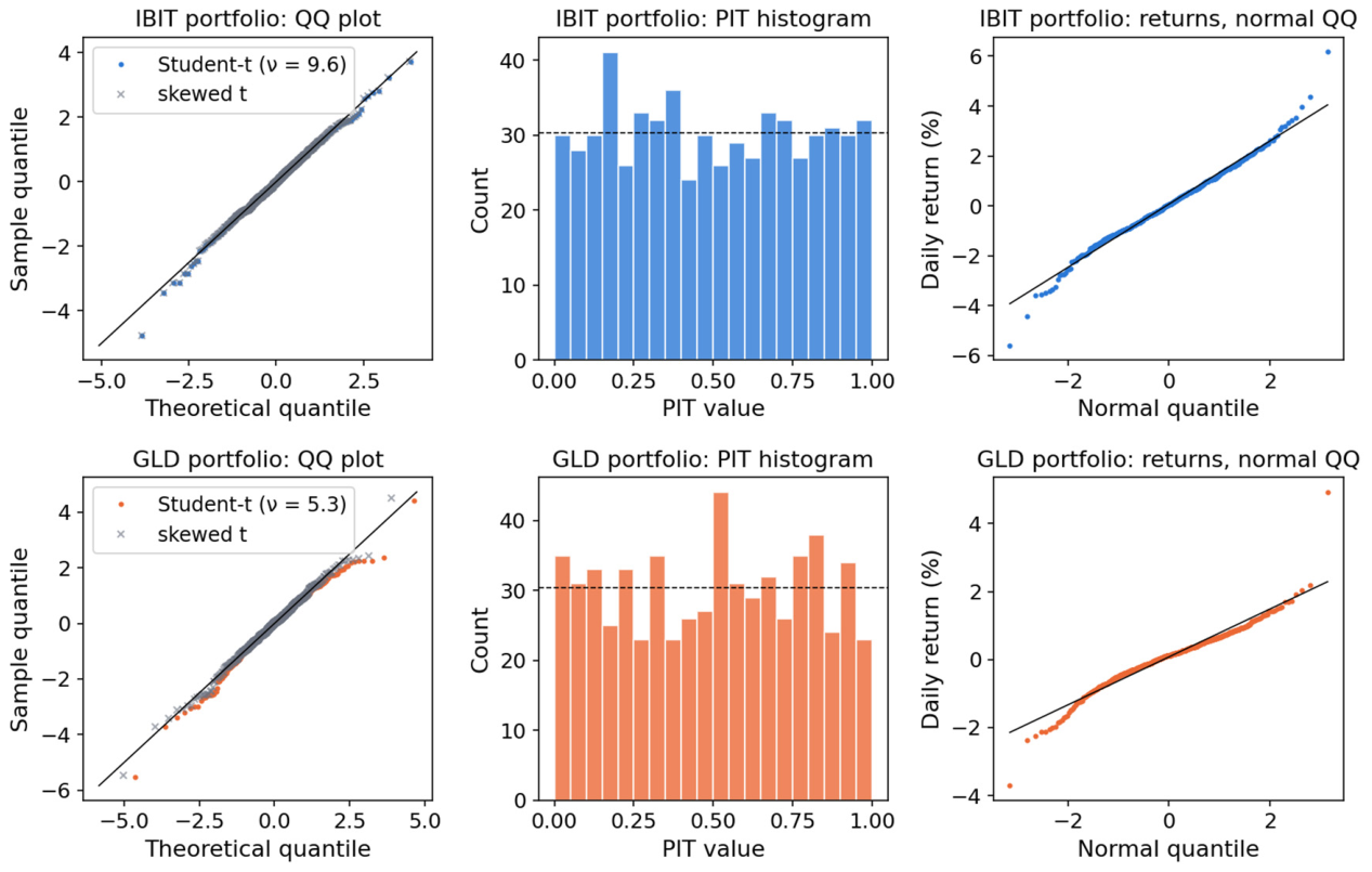
Table A18 examines the mean specification of the GARCH models. The standardized residuals of the IBIT portfolio show serial correlation at 10 and 20 lags (Ljung–Box p = 0.038 and 0.001). The first-order autocorrelation is small and negative (about −0.09 for IBIT) and is shared by Bitcoin priced at 16:00 ET, the reference time of IBIT’s benchmark, but is weaker for BTC-USD at 00:00 UTC; it is therefore a property of Bitcoin’s price at the U.S. close in this period rather than of the ETF. An AR(1) mean does not remove the autocorrelation at 20 lags, is not supported by the BIC, and leaves the tail comparison unchanged: the GARCH-standardized shape ratio is 0.881 with a constant mean and 0.887 with an AR(1) mean. Out of sample, the AR(1) mean changes one backtest decision in the ETF sample at the 5% level (Section 4.3). Over 2014–2026 the AR(1) coefficient of Bitcoin, estimated under the Student-t likelihood, is small (−0.03) and does not reduce the autocorrelation of the standardized residuals. The squared standardized residuals show no remaining conditional heteroskedasticity.
Table A18.
GARCH(1,1)-t with constant and AR(1) mean: Residual diagnostics and model choice.
Appendix D
Source and snapshot. Daily open, high, low, close, adjusted close and volume for IBIT, GLD, TLT and SPY, the VIX and BTC-USD were downloaded from Yahoo Finance on 21 September 2026 at 08:29 UTC. The raw responses and the parsed files are archived with a manifest of SHA-256 checksums, and every later step reads only these files, because Yahoo recomputes the whole history of adjusted prices after each new distribution. Two further snapshots taken on the same day for the supplementary data sets have identical closing prices and adjusted closing prices that differ by at most $0.0002. The 608 closing prices from 11 January 2024, IBIT’s first trading day, to 15 June 2026 give 607 daily returns from 12 January 2024.
Distributions and splits. Returns are computed from adjusted closing prices, which account for splits and distributions. IBIT and GLD are grantor trusts that made no distributions during the sample, so their adjusted and unadjusted prices coincide; TLT made 29 and SPY nine distributions, and unadjusted prices would understate their annual returns by 4.14 and 1.37 percentage points. The multiplicative adjustment is equivalent to reinvesting each distribution at the close before the ex-date; reinvesting at the ex-date close instead, as in CRSP total returns, changes annual returns by at most 0.001 percentage points. Every distribution was matched to the jump in the ratio of adjusted to unadjusted prices (largest discrepancy $0.0001). None of the four ETFs split during the sample; for the splits among the other ETFs (ARKB, 3-for-1 on 16 June 2025, split-date return +3.39%; HODL, 4-for-1 on 14 February 2025, split-date return +1.15%) the split-date returns confirm that the prices are split-adjusted.
Trading calendar. All series are aligned by an inner join on the SPY trading calendar without forward filling or interpolation. The calendar was checked day by day against the NYSE holiday schedule: none of the 25 full-day closures in the sample period, including the national day of mourning on 9 January 2025, appears in the data, and no trading day is missing. The 6 early-closing sessions (13:00 ET) are retained, as are the 4 days on which the bond market was closed but the stock exchanges were open (Columbus Day and Veterans Day), when TLT still traded. The VIX, which closes at 16:15 ET, is used only as a state variable.
Bitcoin prices. BTC-USD trades around the clock. The vendor’s daily bar dated t covers the UTC day t and closes at 00:00 UTC on t + 1, that is, at 19:00 (EST) or 20:00 (EDT) on U.S. date t, three to four hours after the U.S. close of the same date. Each U.S. trading day is matched with the BTC-USD bar of the same date, and returns are computed from these matched closing prices, so that changes over weekends and holidays accrue to the next trading day’s return. For example, the bar dated Monday 3 March 2025 closes at 00:00 UTC on 4 March (19:00 EST on 3 March) and is matched with SPY’s close of 3 March; the aligned return for that day runs from the close of the bar dated Friday 28 February (19:00 EST on 28 February) and is 86,065.67/84,373.01 − 1 = +2.01%. It includes the weekend moves (+1.97% and +9.55%) as well as Monday’s (−8.68%); dropping the weekend days from a series of calendar-day returns would instead have given −8.68%. The three- to four-hour offset lowers the daily correlation between IBIT and BTC-USD to 0.905, whereas their weekly correlation is 0.991 and the correlations of IBIT with the previous and the next day’s BTC-USD return are −0.01 and −0.05; the daily gap reflects the closing time rather than tracking error (Section 4.8). The annualized log return of IBIT differs from that of BTC-USD by −0.36% over the sample, consistent with the fee and noise from the closing time. All main results use ETF prices, which close at the same time.
Data quality. After alignment there are no missing values, duplicate dates or inconsistent open, high, low and close prices. Returns are neither winsorized nor trimmed; three daily returns lie more than five standard deviations from the mean and are retained: GLD on 30 January 2026 (−10.3%) and SPY on 4 April 2025 (−5.9%) and 9 April 2025 (+10.5%).
Fees and the risk-free rate. Management fees accrue daily against net assets and are reflected in prices, so all returns are net of fees and no further deduction is made. The sponsor fees are 0.25% for IBIT (reduced to 0.12% on the first $5 billion of assets for the 12 months from 11 January 2024), 0.40% for GLD, 0.15% for TLT and 0.0945% for SPY; those of the other funds are listed in Table A7. The risk-free rate is the 13-week Treasury bill rate (CBOE index ^IRX), whose sample average is 4.32% on the quoted discount basis and 4.44% as a bond-equivalent yield. The main text uses a constant 4.3% a year. Using instead the previous day’s bond-equivalent yield, converted to a daily rate, changes the annualized Sharpe ratios of the four ETFs by at most 0.01 (Table A19); the long-sample portfolio analysis (Section 4.7) and the cost analysis (Appendix H) use the daily rate. The standard errors of the Sharpe ratios under independent returns (Lo, 2002) are 0.64–0.65.
Simple and log returns. Simple returns are used throughout, including in the GARCH models, because portfolio returns aggregate linearly only in simple returns. Table A19 reports the skewness and excess kurtosis under both definitions.
Revision snapshots. For the second revision, the Bitcoin long-sample snapshot (September 2014–June 2026) was downloaded again on 21 October 2026, and a gold and equity snapshot starting in January 2000 (gold futures, GLD, SPY, TLT, the S&P 500 index, the VIX and the 13-week Treasury bill rate) was added on the same day. For the series without distributions (IBIT, GLD, the VIX and the bill rate) the re-downloaded files are byte-for-byte identical to those of September 2026, and the ETF-sample files are identical except for the adjusted prices of SPY and TLT, which the vendor rescales after each new distribution. These differences change daily returns by less than 10−5; every result of the first revision that was recomputed from the new snapshots (including the ES ratios and their intervals, the stress scenarios and the episode returns) is unchanged at the reported precision.
Table A19.
Data checks for the four ETFs, 12 January 2024–15 June 2026 (607 daily returns).
Table A20 summarizes the structure of the two funds studied, from their prospectuses and annual reports. Both shares are beneficial interests in trusts, redeemable for the underlying asset only by authorized participants. The funds differ in how the asset is held and in the exposures this creates. IBIT’s Bitcoin is held in segregated cold-storage accounts at its custodian, but the part used for trading is an omnibus claim on the prime execution agent, and all of the trust’s Bitcoin is subject to a lien securing intraday trade credit. GLD’s gold is held as allocated, individually identified bars that are not lent, but gold in transit can be held unallocated, as an unsecured claim on the custodian, and a custodian’s insolvency could delay access. Neither trust insures its assets. These features are documented here because historical prices reflect them only if they caused losses during the sample.
Table A20.
Structure of the two funds studied: Backing, custody, segregation, lending, collateral and redemption.
Appendix E
Table A21, Table A22, Table A23 and Table A24 and Figure A2 and Figure A3 report the sensitivity of the controlled comparison (Section 3.5) to the weight of the substituted sleeve, the rebalancing rule, the period and the risk measure; the sensitivity to the Bitcoin and gold instruments and to the equity and bond legs is reported in Section 4.8, Table 16, Table A4, Table A5, Table A7 and Table A8. Unless stated otherwise, portfolios hold one-third each of the sleeve asset, SPY and TLT, rebalanced daily, and ES is estimated by historical simulation. Intervals are from a stationary block bootstrap with expected block length 2 (2000 replications for IBIT, 1000 for the spot series), as in Section 4.8, so the baseline interval (1.35–1.98) differs slightly from that in Section 4.1. With Bitcoin spot prices, BTC-USD returns are reduced by 0.25% a year to mimic an ETF fee; before 2024 these are hypothetical portfolios. For rebalancing rules other than daily, the spot series is not bootstrapped, because Bitcoin’s cumulative gains make the realized weights depend on the price path (under buy-and-hold the Bitcoin sleeve grows to 96% of the portfolio). The multiverse varies the weight (10%, 20%, 33% and 50%), the rebalancing rule (daily, monthly, quarterly, buy-and-hold), the equity leg (SPY, VTI, VT, QQQ, EFA), the bond leg (TLT, IEF, AGG, SHY, TIP) and the risk measure (VaR95, ES95, ES99, volatility, maximum drawdown).
Table A21.
ES95 ratio of the Bitcoin portfolio to the gold portfolio when both sleeves have the same weight.
Table A22.
ES95 ratio under alternative rebalancing rules (target weights one-third each).
Table A23.
ES95 ratio by period.
Table A24.
Ratio of the IBIT portfolio to the GLD portfolio under alternative risk measures.
Figure A2.
Specification curve: Ratio of the risk measure of the Bitcoin portfolio to that of the gold portfolio (ES95 unless the risk measure is the dimension varied) in 183 related specifications that vary one dimension at a time, with 95% bootstrap intervals (log scale); the lower panel marks the dimension varied. Dashed line: Baseline (1.63).
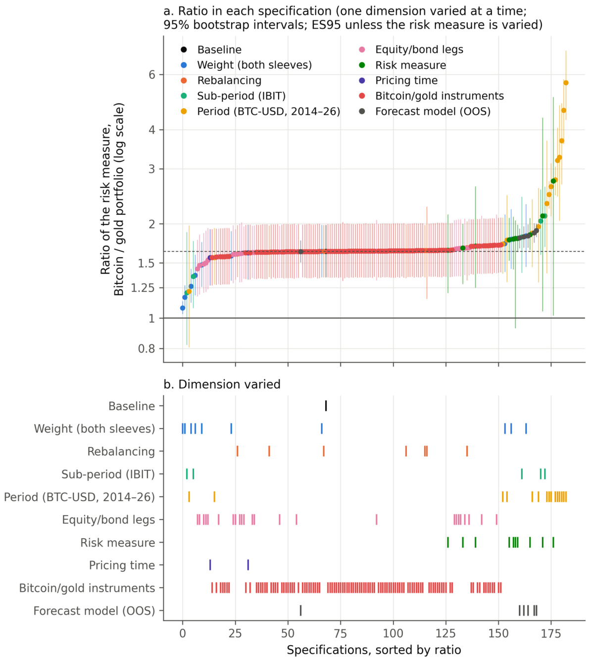
Figure A3.
Daily ES95 of the portfolio of the Bitcoin sleeve, SPY and TLT (the latter two sharing the remainder equally) as a function of the Bitcoin weight (0–50%), with 95% bootstrap bands, against the ES95 of the fixed benchmark of one-third each of GLD, SPY and TLT: (a) IBIT, 2024–2026; (b) Bitcoin spot, 2014–2026. The risk-equivalent weight w* is the crossing on the increasing branch of the curve (see the text below); dashed line: One-third.
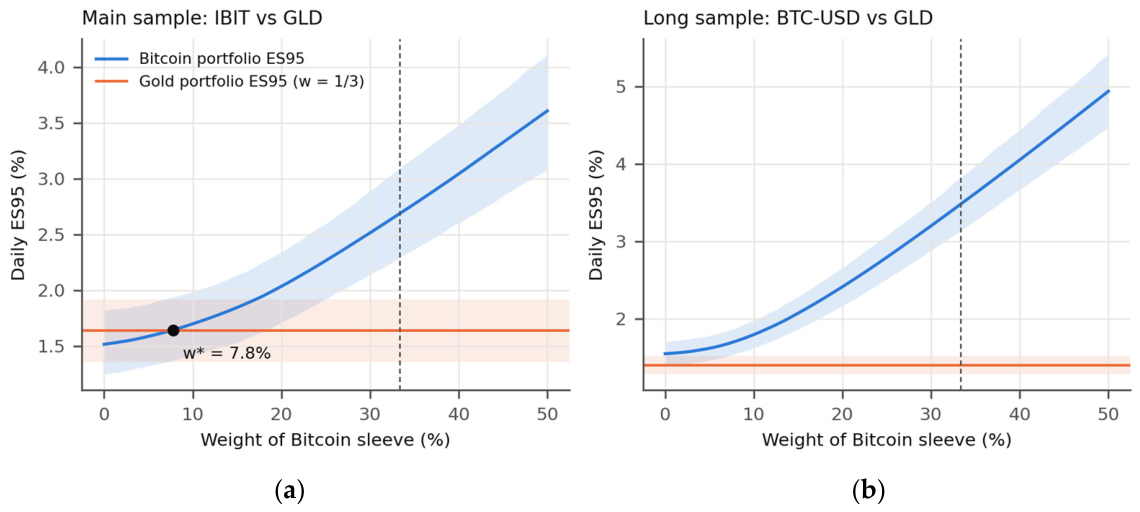
The risk-equivalent weight is defined as follows. For a weight g on a grid from 0 to 50% in steps of 0.5%, the portfolio holds g in IBIT (BTC-USD in the long sample) and (1 − g)/2 each in SPY and TLT, rebalanced daily, and its historical ES95 is compared with that of the fixed benchmark of one-third each of GLD, SPY and TLT. Because ES is convex in the portfolio weights, the ES curve is convex in g; w* is its crossing of the benchmark on the increasing branch, located by linear interpolation between grid points. In the ETF sample the curve is lowest at g = 0 (ES95 1.52% for SPY and TLT alone against 1.64% for the benchmark) and the crossing is unique at 7.8%. In each bootstrap resample (the 2000 resamples of Figure A3, which resample the same days for both portfolios), the crossing exists in 80.6% (in 0.6% the curve also crosses the benchmark on its decreasing branch, and the crossing on the increasing branch is used); in the other 19.4%, the curve lies above the benchmark at every weight, i.e., even the portfolio without Bitcoin has a higher ES95 than the gold portfolio, and no resample has a root above 50% or a numerical failure. The interval 0.7–19.1% is the percentile interval of the resamples with a crossing and is therefore conditional on existence. An unconditional alternative is the set of weights at which the 95% bootstrap interval of the ES95 difference from the benchmark contains zero: 0–18.5%. On rolling 250-day windows, re-estimated every 21 days, a crossing exists in five of 18 windows (at 0.2% to 21.9%); over 2014–2026 it exists neither in the full sample nor in any resample, and in 21% of rolling windows (median 5.2%). The risk-equivalent weight is thus an in-sample calibration of equal estimated risk, not evidence that a stable substitutable allocation exists.
Appendix F
Table A25, Table A26, Table A27 and Table A28 report the conditional-dependence measures summarized in Table 11 for IBIT, GLD and TLT over the ETF sample and for Bitcoin (BTC-USD), GLD and TLT over September 2014–June 2026. Table A25 gives quantile-regression slopes on SPY across the distribution, with kernel-based 95% intervals. Table 11 reports block-bootstrap intervals for the slope at the 0.05 quantile, which are narrower for IBIT, TLT and Bitcoin (for IBIT [1.00, 2.24] against [0.09, 2.13]); with the kernel intervals the slopes of IBIT and of Bitcoin remain significantly positive, whereas that of TLT in the ETF sample does not. Table A26 compares copula families: AIC selects the Gaussian copula for IBIT, whose asymptotic tail dependence is zero, but its finite-quantile λL(5%) is well above the independence value of 0.05, and the families that allow asymmetric lower-tail dependence (Clayton, survival Gumbel) give higher values still. Table A27 reports rank-based tail-dependence coefficients and exceedance correlations with their normal benchmarks, up to one standard deviation, beyond which the ETF sample has fewer than ten joint exceedances. Table A28 reports the DCC regressions, the two-state HMM and the time-varying beta. Non-overlapping two-day returns over 2014–2026 give a correlation of 0.25 between Bitcoin and SPY, λL(5%) = 0.20 (95% CI 0.11–0.30) and a cross-quantilogram of 0.16 (95% CI 0.06–0.27); for GLD the values are 0.12, 0.12 (95% CI 0.04–0.20) and 0.08 (95% CI −0.01 to 0.16).
Table A25.
Quantile-regression slopes on SPY, β(τ), with 95% intervals.
Table A26.
Copula-GARCH models: AIC-selected family and implied lower-tail dependence at the 5% quantile, λL(5%) = C(0.05, 0.05)/0.05.
Table A27.
Tail-dependence coefficients and exceedance correlations with SPY, with 95% intervals.
Table A28.
Dynamic conditional correlation, regime-switching and time-varying-beta models.
Table A29 reports intervals for the copula and DCC measures that include the estimation error of the marginal GARCH models. In a two-stage filtered bootstrap (Pascual et al., 2006), the standardized residual pairs of the asset and SPY are resampled in stationary blocks (expected length 10), two return series are rebuilt with the estimated GARCH recursions, and the GARCH models, the copula and the DCC model are re-estimated in each of 500 replications. Re-estimating the marginal models changes the copula intervals little: relative to the intervals that bootstrap the probability integral transforms, their width changes by a factor of 0.84–1.26, and every λL(5%) remains significantly above its independence value. The DCC intervals widen by a factor of 1.06–2.63 relative to the HAC intervals, which treat the estimated correlation path as known. The tail-day correlations of IBIT and Bitcoin remain significantly positive, whereas those of TLT in the ETF sample and of GLD over 2014–2026 no longer differ significantly from zero. For Bitcoin the full-bootstrap interval lies mostly below the point estimate, because the re-estimated tail-day correlations are on average lower than the original estimate; the percentile interval is reported without bias correction.
Table A29.
Copula and DCC dependence on SPY: 95% confidence intervals conditional on the estimated marginal models and from a two-stage filtered bootstrap that re-estimates them.
Table A30 states what each dependence measure in Table 11 estimates. The measures are complementary and not independent: only the rank-based λL, the cross-quantilogram and the exceedance correlation condition on both returns being in their lower tails, the crisis-regime slope conditions on an estimated regime, and the quantile-regression slope, the DCC correlation and the time-varying beta describe sensitivity or model-implied co-movement over all days. The cross-quantilogram is computed contemporaneously (lag 0) at τ = 0.05, with a tail hit defined as a return strictly below the empirical 5% quantile of its own series; λL(5%) counts days on which both ranks, scaled by n + 1, are at most 0.05. With equal hit counts h for both series, the cross-quantilogram equals (λL − u)/(1 − u) with u = h/n; the two conventions differ by one hit in small samples. In the ETF sample the cross-quantilogram uses 31 hits for each series and eight joint hits for IBIT (five for GLD), and λL uses 30 and seven (4); over 2014–2026 the counts are 148 and 30 for Bitcoin (14 for GLD) against 147 and 29 (14). This accounts for the difference between the cross-quantilogram of IBIT (0.22) and (λL − 0.05)/0.95 = 0.19.
Table A30.
What each dependence measure in Table 11 estimates.
Appendix G
Table A31 specifies the stress-testing protocol, Table A32 lists the dates and results of the 22 historical scenarios, and Table A33 reports the hypothetical scenarios. In the ETF-period scenarios the proxy error—the portfolio return with BTC-USD minus that with IBIT—averages 0.33 percentage points (median absolute value 0.27, maximum 1.41). A 5-basis-point one-way cost on daily rebalancing changes no window return by more than 0.016 percentage points. The weekly regressions behind the hypothetical scenarios are estimated on the 127 weeks of the ETF sample and, for the stressed responses, on the 114 weeks since 2014 with a VIX peak above 25 (with BTC-USD). Because the ETF-sample regressions rest on about two and a half years of weekly data, both sets of responses are reported.
Table A31.
Stress-testing protocol.
Table A32.
Historical stress scenarios: window returns (%) of the assets and of the portfolios.
Table A33.
Hypothetical scenarios: Portfolio returns (%) of the Bitcoin and gold portfolios.
Table A34 reproduces the asset-level episode study of the first version of the paper, which used SPY drawdowns of 8% or more since September 2014 and the realized multiplier of each asset (its return over the episode divided by that of SPY). Bitcoin’s multiplier ranged from −2.77 to +2.83 (standard deviation 1.69) and gold’s from −0.97 to +1.45 (0.64); the ratio of the two dispersions, 2.62, is not significant at the 5% level with nine episodes (95% CI 0.99–4.23; p = 0.054). This dispersion does not indicate an inconsistent response. An asset’s multiplier dispersion grows with its own volatility: under a stable relation with each asset’s full-sample beta and residual variance, the expected ratio of the two dispersions is 4.0, above the observed one, and after each multiplier is scaled by the ratio of SPY’s volatility to the asset’s over the same window the ratio is 0.74. The ratio also depends on single episodes: without the drawdown of 2015–2016 it is 1.41, and without that of January–March 2026 it is 3.72. Bitcoin fell in eight of the nine episodes, and without 2015–2016 its multiplier lies between 0.99 and 2.83: it fell with equities consistently, usually by more.
Table A34.
Equity drawdowns of 8% or more, September 2014–June 2026: Returns from SPY peak to trough (%) and realized multipliers relative to SPY.
Table A35 lists every SPY drawdown episode used in Table 12, Table 13 and Table A34. All three tables now use one convention: an episode is selected by SPY’s drawdown on total-return prices from its running maximum to the trough, with inclusive thresholds, and every window return runs from the close of the peak day to the close of the trough day, so that SPY’s window return equals the drawdown used for selection. The first version computed Table 13 from the close before the peak day and so included the return earned on the peak day itself. As a result, the SPY return reported for a window could be smaller in magnitude than its selection drawdown (−4.56% against −5.35% in March–April 2024), and the episodes common to Table 13 and Table A34 differed by one day and by the peak-day return (for example, −18.56% over 35 days against −18.76% over 34 days in February–April 2025). Under the common convention, each episode has the same SPY return and day count in every table, and each asset return equals both the ratio of the end-point-adjusted prices and the product of the daily gross returns; portfolio returns compound the weighted daily returns under daily rebalancing. The correction changes no conclusion: the IBIT portfolio lost more than the gold portfolio in all five windows of Table 13 (by 4.4 to 8.7 percentage points, against 4.6 to 9.4 before), under daily rebalancing and buy-and-hold alike; the gold portfolio fared worse in the same three of the 28 in-sample scenarios defined by the three window rules of Table A31; and shifting the start and end dates by up to five trading days reverses the portfolio ranking in some windows for the same three of the five events (in at most 40% of the shifted windows, against 45% before).
Table A36 reports severe-state scenarios for the Bitcoin and gold sleeves under stated assumptions. They are not forecasts and carry no probabilities, because the data do not identify the probability of technological displacement, a persistent collapse in demand, a contested change to the protocol or a failure of custody or market access. Each scenario states the sleeve’s loss, its duration, whether it is recovered and whether the sleeve can be traded and rebalanced; SPY and TLT are held flat so that the portfolio outcome isolates the sleeve. The severities are anchored on the deepest historical declines: BTC-USD fell 83% from December 2017 to December 2018 and 77% from November 2021 to November 2022, recovering its previous peak about 2.0 and 1.3 years after the trough, and gold fell 46% from August 2011 to December 2015, recovering in July 2020, 4.6 years later. In the custody or access scenario, the sleeve is frozen—it can be neither traded nor rebalanced—and a fraction of it is recovered later; the portfolio loss is one-third of the unrecovered fraction for either sleeve.
Table A36.
Severe-state scenarios for the Bitcoin and gold sleeves under stated assumptions: portfolio returns (%).
Appendix H
Table A37, Table A38, Table A39 and Table A40 complement Section 4.7. Table A37 gives the in-sample weights of all fifteen strategies of Table 4, with block-bootstrap intervals for the Bitcoin weight (500 replications for IBIT and 300 for the spot series; expected block length 5); expected returns and volatilities are annualized arithmetically. The Ledoit–Wolf shrinkage intensity is 0.11 for IBIT and 0.06 for the spot series, and the Bayes–Stein shrinkage factor φ is 0.51 and 0.34. For the aggressive portfolio the IBIT weight is 0.0%, 0.0%, 0.0%, 1.1% and 3.4% for volatility caps of 10%, 12%, 15%, 17% and 20%. Table A38 reports the allocation, risk and return of Table 15 for the spot series, including the fallback rule of the maximum-Sharpe strategy, Table A39 reports net Sharpe ratios for the nine combinations of estimation window and rebalancing frequency, and Table A40 compares each treatment of estimation error with its sample-estimate counterpart. Figure A4 shows the out-of-sample wealth of selected strategies over 2016–2026 and the Bitcoin weight they choose at each rebalancing.
In the in-sample estimates (Table A37), the maximum-Sharpe portfolio of the ETF sample splits almost evenly between gold and the S&P 500 and the minimum-variance portfolio holds mainly Treasuries; neither holds IBIT. The bootstrap interval for the maximum-Sharpe GLD weight spans almost the whole unit interval (1.5% to 100%), because 607 days are far too few to estimate expected returns, whereas the upper bound of the interval for the IBIT weight is at most 3.2% for minimum variance and minimum CVaR.
Table A37.
In-sample weights of the fifteen strategies (%).
Table A38.
Out-of-sample allocation, risk and return with Bitcoin spot prices (250-day window, rebalanced every 21 days; 13 September 2016–15 June 2026; 10 basis points per unit traded).
Table A39.
Net Sharpe ratios for alternative estimation windows and rebalancing intervals (10 basis points per unit traded).
Table A40.
Do treatments of estimation error help? Paired out-of-sample comparisons (10 basis points per unit traded).
Figure A4.
Out-of-sample strategies with Bitcoin spot prices, September 2016–June 2026 (250-day window, monthly rebalancing, 10 basis points per unit traded): (a) wealth, log scale; (b) Bitcoin weight at each rebalancing.
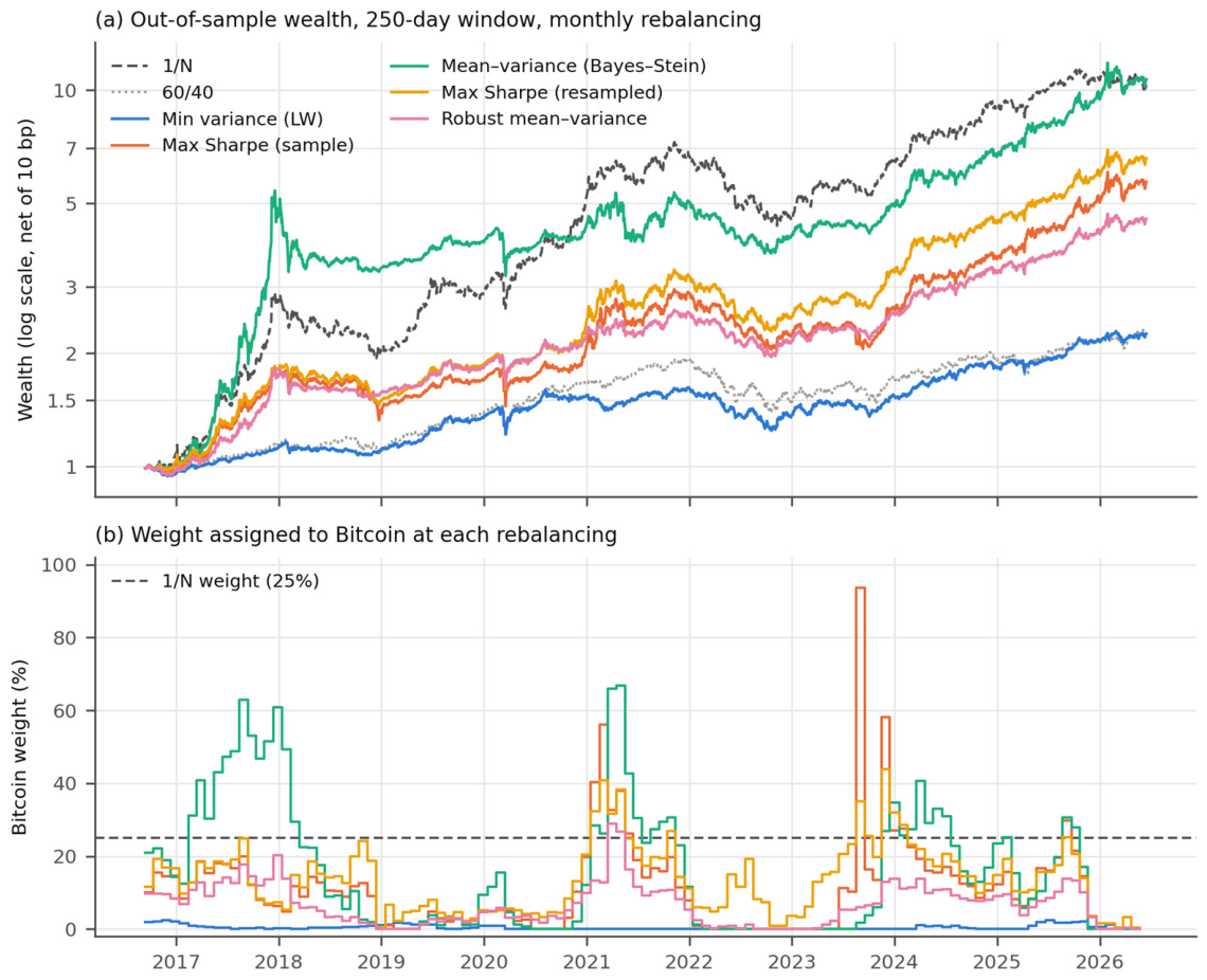
The costs of implementing the portfolios are examined with an explicit model of execution costs. Each trade pays half the quoted spread of one cent (a full spread of 2.2 basis points at IBIT’s median price) plus square-root market impact, Yσ(Q/V)1/2 per unit traded with Y = 1, where σ is the 21-day volatility, Q the dollar amount traded and V the 21-day median daily dollar volume (Almgren et al., 2005). For a conservative execution-cost scenario, effective spreads are estimated from daily high, low and closing prices (Corwin & Schultz, 2012; Abdi & Ranaldo, 2017), and twice that estimate serves as a stressed case; these estimators are noisy and are not formal upper bounds. ETF expense ratios are already reflected in prices and are not deducted again.
Table A41, Table A42, Table A43 and Table A44 report the implementation-cost analysis of Section 4.7 over the full sample (607 days). Portfolios are rebalanced monthly and have $100 million under management unless stated otherwise; the initial purchase is not charged. Sharpe ratios are computed from daily returns in excess of the daily 13-week Treasury bill rate (bond-equivalent yield, Appendix D), so they differ slightly from those computed with a constant 4.3%. Differences in Sharpe ratios are tested with the method of Ledoit and Wolf (2008) and bootstrapped with a paired stationary block bootstrap that resamples the same days for both portfolios. The one-cent spread is the full quoted spread at the median price; the cost model charges half of it per unit traded. The high–low estimators are noisy for very liquid funds; the Abdi–Ranaldo estimate is set to zero when the 21-day average of its squared spreads is negative, which is why some entries in Table A41 are zero, and both are used only in the conservative execution-cost scenario. The break-even extra cost for the 5% IBIT allocation is 552 basis points per unit of IBIT traded.
Table A41.
Liquidity, spreads and fees of the four ETFs, January 2024–June 2026.
Table A42.
Adding IBIT or GLD to a 60/40 SPY–TLT portfolio, after spreads and market impact ($100 million, monthly rebalancing).
Table A43.
Turnover and costs of alternative rebalancing rules ($100 million).
Table A44.
Portfolio size, market impact and capacity (monthly rebalancing).
Table A45 reports the mean–variance spanning tests of Section 4.7. For each test asset the regression on the three benchmark assets is estimated with Newey–West standard errors, and the Wald tests replace the finite-sample F tests, which assume normal and serially independent returns. The two components of the spanning hypothesis are reported separately: δ = 0, which concerns the global-minimum-variance portfolio and involves covariances only, and α = 0, which concerns the tangency portfolio and depends on mean returns, which are imprecisely estimated over samples of our length (Kan & Zhou, 2012). Because the portfolios of the paper are long-only, the table also reports the one-sided test of whether a long position in the test asset lowers the minimum variance (De Roon et al., 2001) and the long-only minimum-variance portfolio itself. The one-sided test refers to the unconstrained minimum-variance portfolio of the benchmark assets: a positive δ means that a small long position in the test asset lowers its variance. This coincides with the long-only condition when that portfolio has no short positions, as in the tests of Bitcoin, but only approximately in the ETF-sample test of gold, where the unconstrained benchmark portfolio holds a short position of 0.5% in IBIT. None of these regression tests determines the optimal allocation under the long-only constraints used elsewhere; the long-only weights in Table A45 are computed directly and are sample estimates.
Table A45.
Mean–variance spanning tests: Does Bitcoin or gold expand the opportunity set of the other three assets?
Appendix I
Table A46, Table A47, Table A48 and Table A49 document the regime analysis of Section 3.4 and Section 4.4. Table A46 reports the Markov-switching models for SPY. The three-state model is preferred by the BIC; its states are persistent (stay probabilities 0.96–0.97), and transitions occur almost only between adjacent states, so a crisis regime is entered and left through the turbulent regime. The crisis regime covers parts of the dot-com bust of 2000–2002, the global financial crisis (March 2008 to 2009), the euro-area crisis of 2010–2011, the COVID-19 crash (February to June 2020), parts of 2022 and the April 2025 tariff shock (Figure 4).
Table A46.
Markov-switching models for daily SPY returns, August 2000–June 2026.
Table A47 reports all Forbes–Rigobon comparisons, Table A48 the threshold regressions with their sub-period splits, and Table A49 the two-state Markov-switching regressions of each asset on SPY and the crisis slopes with probability weights. Repeating the regime analyses with the filtered classification, which uses returns only up to each day but parameters estimated over the whole sample and is therefore not fully real time, changes no conclusion. With the filtered classification, Bitcoin’s correlation with and slope on SPY in the crisis regime are 0.55 and 1.06 over 2014–2026 (0.51 and 1.01 with the smoothed classification), gold’s are 0.01 and 0.01 over 2002–2026, and the ES95 of the Bitcoin and gold portfolios in the crisis regime is 8.39% and 3.22% (8.49% and 3.22%).
Table A47.
Forbes–Rigobon tests of contagion between equities and Bitcoin, gold and Treasuries.
Table A48.
Threshold regressions of each asset on SPY with the previous day’s VIX as the threshold variable.
Table A49.
Two-state Markov-switching regressions of each asset on SPY, and probability-weighted crisis slopes.
Appendix J
Table A50 lists, for each group of results, how its intervals or p-values are obtained, whether they are conditional on estimated inputs, how multiple comparisons are treated and whether the analysis is confirmatory, exploratory or a robustness check. Adjustments for multiple comparisons are applied where many hypotheses of the same kind are tested against a common benchmark: the 14 alternative strategies against 1/N (Holm, 1979) and the risk models (model confidence set). The specification families, regime definitions and robustness measures are reported together rather than adjusted, and their number is not used as evidence.
Table A50.
Sources of the reported intervals and tests, conditioning on estimated inputs, adjustments for multiple comparisons and status of each analysis.
References
- Abdi, F., & Ranaldo, A. (2017). A simple estimation of bid-ask spreads from daily close, high, and low prices. The Review of Financial Studies, 30(12), 4437–4480. [Google Scholar] [CrossRef] [Scilit]
- Acerbi, C., & Székely, B. (2014). Back-testing expected shortfall. Risk, 27(12), 76–81. [Google Scholar]
- Almgren, R., Thum, C., Hauptmann, E., & Li, H. (2005). Equity market impact. Risk, 18(7), 58–62. [Google Scholar]
- Amihud, Y. (2002). Illiquidity and stock returns: Cross-section and time-series effects. Journal of Financial Markets, 5(1), 31–56. [Google Scholar] [CrossRef] [Scilit]
- Andrews, D. W. K. (2001). Testing when a parameter is on the boundary of the maintained hypothesis. Econometrica, 69(3), 683–734. [Google Scholar] [CrossRef] [Scilit]
- Ang, A., & Bekaert, G. (2002). International asset allocation with regime shifts. The Review of Financial Studies, 15(4), 1137–1187. [Google Scholar] [CrossRef] [Scilit]
- Ang, A., & Chen, J. (2002). Asymmetric correlations of equity portfolios. Journal of Financial Economics, 63(3), 443–494. [Google Scholar] [CrossRef] [Scilit]
- Artzner, P., Delbaen, F., Eber, J.-M., & Heath, D. (1999). Coherent measures of risk. Mathematical Finance, 9(3), 203–228. [Google Scholar] [CrossRef] [Scilit]
- Babalos, V., Bouri, E., & Gupta, R. (2025). Does the introduction of US spot Bitcoin ETFs affect spot returns and volatility of major cryptocurrencies? The Quarterly Review of Economics and Finance, 102, 102006. [Google Scholar] [CrossRef] [Scilit]
- Basel Committee on Banking Supervision. (2019). Minimum capital requirements for market risk. Bank for International Settlements. Available online: https://www.bis.org/bcbs/publ/d457.htm (accessed on 27 September 2026).
- Basel Committee on Banking Supervision. (2022). Prudential treatment of cryptoasset exposures. Bank for International Settlements. Available online: https://www.bis.org/bcbs/publ/d545.htm (accessed on 17 November 2026).
- Baur, D. G. (2013). The structure and degree of dependence: A quantile regression approach. Journal of Banking & Finance, 37(3), 786–798. [Google Scholar] [CrossRef] [Scilit]
- Baur, D. G., Dimpfl, T., & Kuck, K. (2018a). Bitcoin, gold and the US dollar—A replication and extension. Finance Research Letters, 25, 103–110. [Google Scholar] [CrossRef] [Scilit]
- Baur, D. G., Hong, K., & Lee, A. D. (2018b). Bitcoin: Medium of exchange or speculative assets? Journal of International Financial Markets, Institutions and Money, 54, 177–189. [Google Scholar] [CrossRef] [Scilit]
- Baur, D. G., & Lucey, B. M. (2010). Is gold a hedge or a safe haven? An analysis of stocks, bonds and gold. The Financial Review, 45(2), 217–229. [Google Scholar] [CrossRef] [Scilit]
- Baur, D. G., & McDermott, T. K. (2010). Is gold a safe haven? International evidence. Journal of Banking & Finance, 34(8), 1886–1898. [Google Scholar] [CrossRef] [Scilit]
- Beckmann, J., Berger, T., & Czudaj, R. (2015). Does gold act as a hedge or a safe haven for stocks? A smooth transition approach. Economic Modelling, 48, 16–24. [Google Scholar] [CrossRef] [Scilit]
- Berkowitz, J. (2001). Testing density forecasts, with applications to risk management. Journal of Business & Economic Statistics, 19(4), 465–474. [Google Scholar] [CrossRef] [Scilit]
- Bezerra, P. C. S., & Albuquerque, P. H. M. (2017). Volatility forecasting via SVR–GARCH with mixture of Gaussian kernels. Computational Management Science, 14(2), 179–196. [Google Scholar] [CrossRef] [Scilit]
- Biais, B., Bisière, C., Bouvard, M., Casamatta, C., & Menkveld, A. J. (2023). Equilibrium Bitcoin pricing. The Journal of Finance, 78(2), 967–1014. [Google Scholar] [CrossRef] [Scilit]
- Bitcoin Core. (2016, January 7). Statement from Bitcoin Core. Available online: https://bitcoincore.org/en/2016/01/07/statement/ (accessed on 17 November 2026).
- Bollerslev, T. (1986). Generalized autoregressive conditional heteroskedasticity. Journal of Econometrics, 31(3), 307–327. [Google Scholar] [CrossRef] [Scilit]
- Bollerslev, T. (1987). A conditionally heteroskedastic time series model for speculative prices and rates of return. The Review of Economics and Statistics, 69(3), 542–547. [Google Scholar] [CrossRef] [Scilit]
- Bollerslev, T., & Wooldridge, J. M. (1992). Quasi-maximum likelihood estimation and inference in dynamic models with time-varying covariances. Econometric Reviews, 11(2), 143–172. [Google Scholar] [CrossRef] [Scilit]
- Boucher, C. M., Daníelsson, J., Kouontchou, P. S., & Maillet, B. B. (2014). Risk models-at-risk. Journal of Banking & Finance, 44, 72–92. [Google Scholar] [CrossRef] [Scilit]
- Bouri, E., Molnár, P., Azzi, G., Roubaud, D., & Hagfors, L. I. (2017). On the hedge and safe haven properties of Bitcoin: Is it really more than a diversifier? Finance Research Letters, 20, 192–198. [Google Scholar] [CrossRef] [Scilit]
- Bouri, E., Shahzad, S. J. H., & Roubaud, D. (2019). Co-explosivity in the cryptocurrency market. Finance Research Letters, 29, 178–183. [Google Scholar] [CrossRef] [Scilit]
- Boyer, B. H., Gibson, M. S., & Loretan, M. (1997). Pitfalls in tests for changes in correlations (International Finance Discussion Papers No. 597). Board of Governors of the Federal Reserve System. Available online: https://www.federalreserve.gov/pubs/ifdp/1997/597 (accessed on 17 November 2026).
- Böhme, R., Christin, N., Edelman, B., & Moore, T. (2015). Bitcoin: Economics, technology, and governance. Journal of Economic Perspectives, 29(2), 213–238. [Google Scholar] [CrossRef] [Scilit]
- Bredin, D., Conlon, T., & Potì, V. (2015). Does gold glitter in the long-run? Gold as a hedge and safe haven across time and investment horizon. International Review of Financial Analysis, 41, 320–328. [Google Scholar] [CrossRef] [Scilit]
- Brière, M., Oosterlinck, K., & Szafarz, A. (2015). Virtual currency, tangible return: Portfolio diversification with bitcoin. Journal of Asset Management, 16(6), 365–373. [Google Scholar] [CrossRef] [Scilit]
- Bukaita, W., & Li, X. (2026). Structural spillovers among Bitcoin, Ethereum, gold, and U.S. equities: Evidence from the 2024 spot ETF institutionalization regime. Economies, 14(4), 143. [Google Scholar] [CrossRef] [Scilit]
- Catania, L., Grassi, S., & Ravazzolo, F. (2019). Forecasting cryptocurrencies under model and parameter instability. International Journal of Forecasting, 35(2), 485–501. [Google Scholar] [CrossRef] [Scilit]
- Ceria, S., & Stubbs, R. A. (2006). Incorporating estimation errors into portfolio selection: Robust portfolio construction. Journal of Asset Management, 7(2), 109–127. [Google Scholar] [CrossRef] [Scilit]
- Chen, Y.-L., & Yang, J. J. (2026). Who leads in price discovery? Trading frictions and return transmission in spot Bitcoin ETFs. Applied Economics Letters. Advance online publication. [Google Scholar] [CrossRef] [Scilit]
- Chibane, M., & Janson, N. (2025). Is Bitcoin the best safe haven against geopolitical risk? Finance Research Letters, 74, 106543. [Google Scholar] [CrossRef] [Scilit]
- Choi, S., & Shin, J. (2022). Bitcoin: An inflation hedge but not a safe haven. Finance Research Letters, 46, 102379. [Google Scholar] [CrossRef] [Scilit] [PubMed]
- Chopra, V. K., & Ziemba, W. T. (1993). The effect of errors in means, variances, and covariances on optimal portfolio choice. The Journal of Portfolio Management, 19(2), 6–11. [Google Scholar] [CrossRef] [Scilit]
- Christoffersen, P., & Gonçalves, S. (2005). Estimation risk in financial risk management. Journal of Risk, 7(3), 1–28. [Google Scholar] [CrossRef] [Scilit]
- Christoffersen, P. F. (1998). Evaluating interval forecasts. International Economic Review, 39(4), 841–862. [Google Scholar] [CrossRef] [Scilit]
- Chu, J., Chan, S., Nadarajah, S., & Osterrieder, J. (2017). GARCH modelling of cryptocurrencies. Journal of Risk and Financial Management, 10(4), 17. [Google Scholar] [CrossRef] [Scilit]
- Conlon, T., & McGee, R. (2020). Safe haven or risky hazard? Bitcoin during the Covid-19 bear market. Finance Research Letters, 35, 101607. [Google Scholar] [CrossRef] [Scilit] [PubMed]
- Corbet, S., Larkin, C., & Lucey, B. (2020). The contagion effects of the COVID-19 pandemic: Evidence from gold and cryptocurrencies. Finance Research Letters, 35, 101554. [Google Scholar] [CrossRef] [Scilit] [PubMed]
- Corbet, S., Meegan, A., Larkin, C., Lucey, B., & Yarovaya, L. (2018). Exploring the dynamic relationships between cryptocurrencies and other financial assets. Economics Letters, 165, 28–34. [Google Scholar] [CrossRef] [Scilit]
- Corsetti, G., Pericoli, M., & Sbracia, M. (2005). ‘Some contagion, some interdependence’: More pitfalls in tests of financial contagion. Journal of International Money and Finance, 24(8), 1177–1199. [Google Scholar] [CrossRef] [Scilit]
- Corwin, S. A., & Schultz, P. (2012). A simple way to estimate bid-ask spreads from daily high and low prices. The Journal of Finance, 67(2), 719–760. [Google Scholar] [CrossRef] [Scilit]
- Danielsson, J., James, K. R., Valenzuela, M., & Zer, I. (2016). Model risk of risk models. Journal of Financial Stability, 23, 79–91. [Google Scholar] [CrossRef] [Scilit]
- DeMiguel, V., Garlappi, L., & Uppal, R. (2009). Optimal versus naive diversification: How inefficient is the 1/N portfolio strategy? The Review of Financial Studies, 22(5), 1915–1953. [Google Scholar] [CrossRef] [Scilit]
- De Roon, F. A., Nijman, T. E., & Werker, B. J. M. (2001). Testing for mean-variance spanning with short sales constraints and transaction costs: The case of emerging markets. The Journal of Finance, 56(2), 721–742. [Google Scholar] [CrossRef] [Scilit]
- Diebold, F. X., & Mariano, R. S. (1995). Comparing predictive accuracy. Journal of Business & Economic Statistics, 13(3), 253–263. [Google Scholar] [CrossRef] [Scilit]
- Diebold, F. X., & Yilmaz, K. (2012). Better to give than to receive: Predictive directional measurement of volatility spillovers. International Journal of Forecasting, 28(1), 57–66. [Google Scholar] [CrossRef] [Scilit]
- Dimson, E. (1979). Risk measurement when shares are subject to infrequent trading. Journal of Financial Economics, 7(2), 197–226. [Google Scholar] [CrossRef] [Scilit]
- Do, K.-O. (2026). Maturation of Bitcoin market microstructure: Evidence of institutional-grade liquidity and efficiency (2012–2025). Borsa Istanbul Review, 26(5), 100869. [Google Scholar] [CrossRef] [Scilit]
- Durbin, J., & Koopman, S. J. (2012). Time series analysis by state space methods (2nd ed.). Oxford University Press. [Google Scholar] [CrossRef] [Scilit]
- Dyhrberg, A. H. (2016). Bitcoin, gold and the dollar—A GARCH volatility analysis. Finance Research Letters, 16, 85–92. [Google Scholar] [CrossRef] [Scilit]
- Efron, B. (1987). Better bootstrap confidence intervals. Journal of the American Statistical Association, 82(397), 171–185. [Google Scholar] [CrossRef]
- Elton, E. J., Gruber, M. J., Comer, G., & Li, K. (2002). Spiders: Where are the bugs? The Journal of Business, 75(3), 453–472. [Google Scholar] [CrossRef] [Scilit] [PubMed]
- Engle, R. (2002). Dynamic conditional correlation: A simple class of multivariate generalized autoregressive conditional heteroskedasticity models. Journal of Business & Economic Statistics, 20(3), 339–350. [Google Scholar] [CrossRef] [Scilit]
- Engle, R. F., Ghysels, E., & Sohn, B. (2013). Stock market volatility and macroeconomic fundamentals. The Review of Economics and Statistics, 95(3), 776–797. [Google Scholar] [CrossRef] [Scilit]
- Engle, R. F., & Manganelli, S. (2004). CAViaR: Conditional autoregressive value at risk by regression quantiles. Journal of Business & Economic Statistics, 22(4), 367–381. [Google Scholar] [CrossRef] [Scilit]
- Erb, C. B., & Harvey, C. R. (2013). The golden dilemma. Financial Analysts Journal, 69(4), 10–42. [Google Scholar] [CrossRef] [Scilit]
- Fissler, T., & Ziegel, J. F. (2016). Higher order elicitability and Osband’s principle. The Annals of Statistics, 44(4), 1680–1707. [Google Scholar] [CrossRef] [Scilit]
- Forbes, K. J., & Rigobon, R. (2002). No contagion, only interdependence: Measuring stock market comovements. The Journal of Finance, 57(5), 2223–2261. [Google Scholar] [CrossRef] [Scilit]
- Giacomini, R., & White, H. (2006). Tests of conditional predictive ability. Econometrica, 74(6), 1545–1578. [Google Scholar] [CrossRef] [Scilit]
- Gneiting, T. (2011). Making and evaluating point forecasts. Journal of the American Statistical Association, 106(494), 746–762. [Google Scholar] [CrossRef] [Scilit]
- Goldfarb, D., & Iyengar, G. (2003). Robust portfolio selection problems. Mathematics of Operations Research, 28(1), 1–38. [Google Scholar] [CrossRef] [Scilit]
- Guidolin, M., & Timmermann, A. (2007). Asset allocation under multivariate regime switching. Journal of Economic Dynamics and Control, 31(11), 3503–3544. [Google Scholar] [CrossRef] [Scilit]
- Hamilton, J. D. (1989). A new approach to the economic analysis of nonstationary time series and the business cycle. Econometrica, 57(2), 357–384. [Google Scholar] [CrossRef] [Scilit]
- Han, H., Linton, O., Oka, T., & Whang, Y.-J. (2016). The cross-quantilogram: Measuring quantile dependence and testing directional predictability between time series. Journal of Econometrics, 193(1), 251–270. [Google Scholar] [CrossRef] [Scilit]
- Hansen, B. E. (1994). Autoregressive conditional density estimation. International Economic Review, 35(3), 705–730. [Google Scholar] [CrossRef] [Scilit]
- Hansen, B. E. (1996). Inference when a nuisance parameter is not identified under the null hypothesis. Econometrica, 64(2), 413–430. [Google Scholar] [CrossRef] [Scilit]
- Hansen, B. E. (2000). Sample splitting and threshold estimation. Econometrica, 68(3), 575–603. [Google Scholar] [CrossRef] [Scilit]
- Hansen, P. R., & Lunde, A. (2005). A forecast comparison of volatility models: Does anything beat a GARCH(1,1)? Journal of Applied Econometrics, 20(7), 873–889. [Google Scholar] [CrossRef] [Scilit]
- Hansen, P. R., Lunde, A., & Nason, J. M. (2011). The model confidence set. Econometrica, 79(2), 453–497. [Google Scholar] [CrossRef] [Scilit]
- Hill, B. M. (1975). A simple general approach to inference about the tail of a distribution. The Annals of Statistics, 3(5), 1163–1174. [Google Scholar] [CrossRef] [Scilit]
- Holm, S. (1979). A simple sequentially rejective multiple test procedure. Scandinavian Journal of Statistics, 6(2), 65–70. [Google Scholar]
- Hong, Y., Feng, H., Wang, Y., & Li, B. (2025). The impact of Bitcoin ETF approval on Bitcoin’s hedging properties against traditional assets. arXiv, arXiv:2512.12815. [Google Scholar] [CrossRef] [Scilit]
- Hong, Y., Tu, J., & Zhou, G. (2007). Asymmetries in stock returns: Statistical tests and economic evaluation. The Review of Financial Studies, 20(5), 1547–1581. [Google Scholar] [CrossRef] [Scilit]
- Hood, M., & Malik, F. (2013). Is gold the best hedge and a safe haven under changing stock market volatility? Review of Financial Economics, 22(2), 47–52. [Google Scholar] [CrossRef] [Scilit]
- Hornback, A. M., & Whaley, R. E. (2025). Spot Bitcoin ETFs: The struggle was worth it. Financial Analysts Journal, 81(2), 39–50. [Google Scholar] [CrossRef] [Scilit]
- Huberman, G., & Kandel, S. (1987). Mean-variance spanning. The Journal of Finance, 42(4), 873–888. [Google Scholar] [CrossRef]
- Hwang, S., & Valls Pereira, P. L. (2006). Small sample properties of GARCH estimates and persistence. The European Journal of Finance, 12(6–7), 473–494. [Google Scholar] [CrossRef] [Scilit]
- iShares Bitcoin Trust ETF. (2025). Prospectus (July 31, 2025; Supplement No. 1, November 21, 2025). U.S. Securities and Exchange Commission. Available online: https://www.sec.gov/Archives/edgar/data/1980994/000143774925024228/bit20250731_424b3.htm (accessed on 17 November 2026).
- iShares Bitcoin Trust ETF. (2026). Annual report on Form 10-K for the fiscal year ended December 31, 2025. U.S. Securities and Exchange Commission. Available online: https://www.sec.gov/Archives/edgar/data/1980994/000143774926006058/bit20251231_10k.htm (accessed on 17 November 2026).
- Ji, Q., Bouri, E., Lau, C. K. M., & Roubaud, D. (2019). Dynamic connectedness and integration in cryptocurrency markets. International Review of Financial Analysis, 63, 257–272. [Google Scholar] [CrossRef] [Scilit]
- Jorion, P. (1986). Bayes–Stein estimation for portfolio analysis. Journal of Financial and Quantitative Analysis, 21(3), 279–292. [Google Scholar] [CrossRef] [Scilit]
- Jorion, P. (2007). Value at risk: The new benchmark for managing financial risk (3rd ed.). McGraw-Hill. [Google Scholar]
- Kajtazi, A., & Moro, A. (2019). The role of bitcoin in well diversified portfolios: A comparative global study. International Review of Financial Analysis, 61, 143–157. [Google Scholar] [CrossRef] [Scilit]
- Kan, R., & Zhou, G. (2007). Optimal portfolio choice with parameter uncertainty. Journal of Financial and Quantitative Analysis, 42(3), 621–656. [Google Scholar] [CrossRef] [Scilit]
- Kan, R., & Zhou, G. (2012). Tests of mean-variance spanning. Annals of Economics and Finance, 13(1), 145–193. [Google Scholar]
- Katsiampa, P. (2017). Volatility estimation for Bitcoin: A comparison of GARCH models. Economics Letters, 158, 3–6. [Google Scholar] [CrossRef] [Scilit]
- Kim, H. Y., & Won, C. H. (2018). Forecasting the volatility of stock price index: A hybrid model integrating LSTM with multiple GARCH-type models. Expert Systems with Applications, 103, 25–37. [Google Scholar] [CrossRef] [Scilit]
- Klein, T., Pham Thu, H., & Walther, T. (2018). Bitcoin is not the new gold – A comparison of volatility, correlation, and portfolio performance. International Review of Financial Analysis, 59, 105–116. [Google Scholar] [CrossRef] [Scilit]
- Koenker, R., & Bassett, G. (1978). Regression quantiles. Econometrica, 46(1), 33–50. [Google Scholar] [CrossRef] [Scilit]
- Koenker, R., & Hallock, K. F. (2001). Quantile regression. Journal of Economic Perspectives, 15(4), 143–156. [Google Scholar] [CrossRef] [Scilit]
- Kristjanpoller, W., & Minutolo, M. C. (2015). Gold price volatility: A forecasting approach using the Artificial Neural Network–GARCH model. Expert Systems with Applications, 42(20), 7245–7251. [Google Scholar] [CrossRef] [Scilit]
- Kupiec, P. H. (1995). Techniques for verifying the accuracy of risk measurement models. The Journal of Derivatives, 3(2), 73–84. [Google Scholar] [CrossRef] [Scilit]
- Lakens, D. (2017). Equivalence tests: A practical primer for t tests, correlations, and meta-analyses. Social Psychological and Personality Science, 8(4), 355–362. [Google Scholar] [CrossRef] [Scilit] [PubMed]
- Ledoit, O., & Wolf, M. (2004). Honey, I shrunk the sample covariance matrix. The Journal of Portfolio Management, 30(4), 110–119. [Google Scholar] [CrossRef] [Scilit]
- Ledoit, O., & Wolf, M. (2008). Robust performance hypothesis testing with the Sharpe ratio. Journal of Empirical Finance, 15(5), 850–859. [Google Scholar] [CrossRef] [Scilit]
- Lee, S., & Lee, J. (2025). Shifting dynamics: Bitcoin spot ETF approval and Bitcoin’s relationships with financial markets. Applied Economics Letters. Advance online publication. [Google Scholar] [CrossRef] [Scilit]
- Liu, P., & Yuan, Y. (2024). Is Bitcoin a hedge or safe-haven asset during the period of turmoil? Evidence from the currency, bond and stock markets. International Review of Financial Analysis, 96, 103663. [Google Scholar] [CrossRef] [Scilit]
- Liu, S., & Yang, C. (2024). Spot cryptocurrency ETFs: Crypto investment products or stepping stones toward tokenization. Finance Research Letters, 69, 106150. [Google Scholar] [CrossRef] [Scilit]
- Liu, Y., & Tsyvinski, A. (2021). Risks and returns of cryptocurrency. The Review of Financial Studies, 34(6), 2689–2727. [Google Scholar] [CrossRef] [Scilit]
- Ljung, G. M., & Box, G. E. P. (1978). On a measure of lack of fit in time series models. Biometrika, 65(2), 297–303. [Google Scholar] [CrossRef]
- Lo, A. W. (2002). The statistics of Sharpe ratios. Financial Analysts Journal, 58(4), 36–52. [Google Scholar] [CrossRef] [Scilit]
- Longin, F., & Solnik, B. (2001). Extreme correlation of international equity markets. The Journal of Finance, 56(2), 649–676. [Google Scholar] [CrossRef] [Scilit]
- López de Prado, M. (2016). Building diversified portfolios that outperform out of sample. The Journal of Portfolio Management, 42(4), 59–69. [Google Scholar] [CrossRef] [Scilit]
- López de Prado, M. (2018). Advances in financial machine learning. Wiley. [Google Scholar]
- Maillard, S., Roncalli, T., & Teïletche, J. (2010). The properties of equally weighted risk contribution portfolios. The Journal of Portfolio Management, 36(4), 60–70. [Google Scholar] [CrossRef] [Scilit]
- Markowitz, H. (1952). Portfolio selection. The Journal of Finance, 7(1), 77–91. [Google Scholar] [CrossRef] [Scilit]
- Marti, R., & Reimat, A. (2025). Bitcoin and global stock portfolio: Dynamics across short and long-term horizons. Finance Research Letters, 86, 108918. [Google Scholar] [CrossRef] [Scilit]
- McNeil, A. J., & Frey, R. (2000). Estimation of tail-related risk measures for heteroscedastic financial time series: An extreme value approach. Journal of Empirical Finance, 7(3–4), 271–300. [Google Scholar] [CrossRef] [Scilit]
- McNeil, A. J., Frey, R., & Embrechts, P. (2015). Quantitative risk management: Concepts, techniques and tools (Rev. ed.). Princeton University Press. [Google Scholar]
- Mehdian, S. M., Gherghina, Ș. C., & Stoica, O. (2025). The reaction of cryptocurrencies to the approval of spot Bitcoin and Ethereum ETFs: An intraday event study. Borsa Istanbul Review, 25(6), 1507–1517. [Google Scholar] [CrossRef] [Scilit]
- Michaud, R. O. (1989). The Markowitz optimization enigma: Is ‘optimized’ optimal? Financial Analysts Journal, 45(1), 31–42. [Google Scholar] [CrossRef] [Scilit]
- Michaud, R. O. (1998). Efficient asset management: A practical guide to stock portfolio optimization and asset allocation. Harvard Business School Press. [Google Scholar]
- Mohamad, A. (2025). Do Bitcoin ETFs lead price discovery following their introduction in the Bitcoin market? Computational Economics, 66(1), 947–969. [Google Scholar] [CrossRef] [Scilit]
- Nakamoto, S. (2008). Bitcoin: A peer-to-peer electronic cash system. Available online: https://bitcoin.org/bitcoin.pdf (accessed on 27 September 2026).
- Newey, W. K., & West, K. D. (1987). A simple, positive semi-definite, heteroskedasticity and autocorrelation consistent covariance matrix. Econometrica, 55(3), 703–708. [Google Scholar] [CrossRef] [Scilit]
- Nolde, N., & Ziegel, J. F. (2017). Elicitability and backtesting: Perspectives for banking regulation. The Annals of Applied Statistics, 11(4), 1833–1874. [Google Scholar] [CrossRef] [Scilit]
- Oefele, N. (2025). One year of bitcoin spot ETPs: A brief market and fund flow analysis. Economics Letters, 250, 112304. [Google Scholar] [CrossRef] [Scilit]
- Pascual, L., Romo, J., & Ruiz, E. (2006). Bootstrap prediction for returns and volatilities in GARCH models. Computational Statistics & Data Analysis, 50(9), 2293–2312. [Google Scholar] [CrossRef] [Scilit]
- Pastorek, D., & Albrecht, P. (2026). Risk without reward? The introduction of Bitcoin spot ETFs. Ekonomický časopis, 74(5–6), 215–243. [Google Scholar] [CrossRef] [Scilit]
- Patton, A. J. (2006). Modelling asymmetric exchange rate dependence. International Economic Review, 47(2), 527–556. [Google Scholar] [CrossRef] [Scilit]
- Patton, A. J. (2011). Volatility forecast comparison using imperfect volatility proxies. Journal of Econometrics, 160(1), 246–256. [Google Scholar] [CrossRef] [Scilit]
- Patton, A. J., Ziegel, J. F., & Chen, R. (2019). Dynamic semiparametric models for expected shortfall (and Value-at-Risk). Journal of Econometrics, 211(2), 388–413. [Google Scholar] [CrossRef] [Scilit]
- Petajisto, A. (2017). Inefficiencies in the pricing of exchange-traded funds. Financial Analysts Journal, 73(1), 24–54. [Google Scholar] [CrossRef] [Scilit]
- Platanakis, E., & Urquhart, A. (2020). Should investors include Bitcoin in their portfolios? A portfolio theory approach. The British Accounting Review, 52(4), 100837. [Google Scholar] [CrossRef] [Scilit]
- Politis, D. N., & Romano, J. P. (1994). The stationary bootstrap. Journal of the American Statistical Association, 89(428), 1303–1313. [Google Scholar] [CrossRef]
- Politis, D. N., & White, H. (2004). Automatic block-length selection for the dependent bootstrap. Econometric Reviews, 23(1), 53–70. [Google Scholar] [CrossRef] [Scilit]
- Reboredo, J. C. (2013). Is gold a safe haven or a hedge for the US dollar? Implications for risk management. Journal of Banking & Finance, 37(8), 2665–2676. [Google Scholar] [CrossRef] [Scilit]
- Rockafellar, R. T., & Uryasev, S. (2000). Optimization of conditional value-at-risk. Journal of Risk, 2(3), 21–41. [Google Scholar] [CrossRef] [Scilit]
- Rodriguez, J. C. (2007). Measuring financial contagion: A copula approach. Journal of Empirical Finance, 14(3), 401–423. [Google Scholar] [CrossRef] [Scilit]
- Scholes, M., & Williams, J. (1977). Estimating betas from nonsynchronous data. Journal of Financial Economics, 5(3), 309–327. [Google Scholar] [CrossRef] [Scilit]
- Schuirmann, D. J. (1987). A comparison of the two one-sided tests procedure and the power approach for assessing the equivalence of average bioavailability. Journal of Pharmacokinetics and Biopharmaceutics, 15(6), 657–680. [Google Scholar] [CrossRef] [Scilit] [PubMed]
- Shahzad, S. J. H., Bouri, E., Roubaud, D., & Kristoufek, L. (2020). Safe haven, hedge and diversification for G7 stock markets: Gold versus bitcoin. Economic Modelling, 87, 212–224. [Google Scholar] [CrossRef] [Scilit]
- Simonsohn, U., Simmons, J. P., & Nelson, L. D. (2020). Specification curve analysis. Nature Human Behaviour, 4(11), 1208–1214. [Google Scholar] [CrossRef] [Scilit] [PubMed]
- Smales, L. A. (2019). Bitcoin as a safe haven: Is it even worth considering? Finance Research Letters, 30, 385–393. [Google Scholar] [CrossRef] [Scilit]
- Smith, R. L. (1987). Estimating tails of probability distributions. The Annals of Statistics, 15(3), 1174–1207. [Google Scholar] [CrossRef] [Scilit]
- Sodnomdavaa, T. (2026). Bitcoin and gold causality across quantiles, frequencies, and market regimes. Journal of Risk and Financial Management, 19(3), 215. [Google Scholar] [CrossRef] [Scilit]
- SPDR Gold Trust. (2022). Prospectus (October 4, 2022). U.S. Securities and Exchange Commission. Available online: https://www.sec.gov/Archives/edgar/data/1222333/000119312522257655/d236982d424b3.htm (accessed on 17 November 2026).
- SPDR Gold Trust. (2025). Annual report on Form 10-K for the fiscal year ended September 30, 2025. U.S. Securities and Exchange Commission. Available online: https://www.sec.gov/Archives/edgar/data/1222333/000143774925036305/gld20250930_10k.htm (accessed on 17 November 2026).
- Stavroyiannis, S. (2018). Value-at-risk and related measures for the Bitcoin. The Journal of Risk Finance, 19(2), 127–136. [Google Scholar] [CrossRef] [Scilit]
- Steegen, S., Tuerlinckx, F., Gelman, A., & Vanpaemel, W. (2016). Increasing transparency through a multiverse analysis. Perspectives on Psychological Science, 11(5), 702–712. [Google Scholar] [CrossRef] [Scilit] [PubMed]
- Troster, V., Tiwari, A. K., Shahbaz, M., & Macedo, D. N. (2019). Bitcoin returns and risk: A general GARCH and GAS analysis. Finance Research Letters, 30, 187–193. [Google Scholar] [CrossRef] [Scilit]
- Urquhart, A. (2016). The inefficiency of Bitcoin. Economics Letters, 148, 80–82. [Google Scholar] [CrossRef] [Scilit]
- Urquhart, A., & Zhang, H. (2019). Is Bitcoin a hedge or safe haven for currencies? An intraday analysis. International Review of Financial Analysis, 63, 49–57. [Google Scholar] [CrossRef] [Scilit]
- U.S. Geological Survey. (2026). Gold. In Mineral commodity summaries 2026. U.S. Geological Survey. Available online: https://pubs.usgs.gov/periodicals/mcs2026/mcs2026-gold.pdf (accessed on 17 November 2026).
- U.S. Securities and Exchange Commission. (2024). Order granting accelerated approval of proposed rule changes, as modified by amendments thereto, to list and trade bitcoin-based commodity-based trust shares and trust units (Release No. 34-99306). Available online: https://www.sec.gov/files/rules/sro/nysearca/2024/34-99306.pdf (accessed on 27 September 2026).
- U.S. Securities and Exchange Commission. (2025, July 29). SEC permits in-kind creations and redemptions for crypto ETPs (Press release No. 2025-101). Available online: https://www.sec.gov/newsroom/press-releases/2025-101-sec-permits-kind-creations-redemptions-crypto-etps (accessed on 17 November 2026).
- Wu, D. (2025). Institutional adoption and correlation dynamics: Bitcoin’s evolving role in financial markets. arXiv, arXiv:2501.09911. [Google Scholar] [CrossRef] [Scilit]
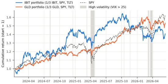
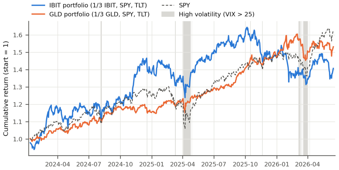
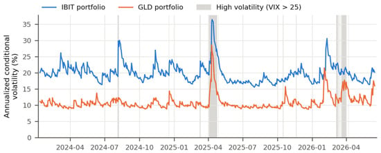
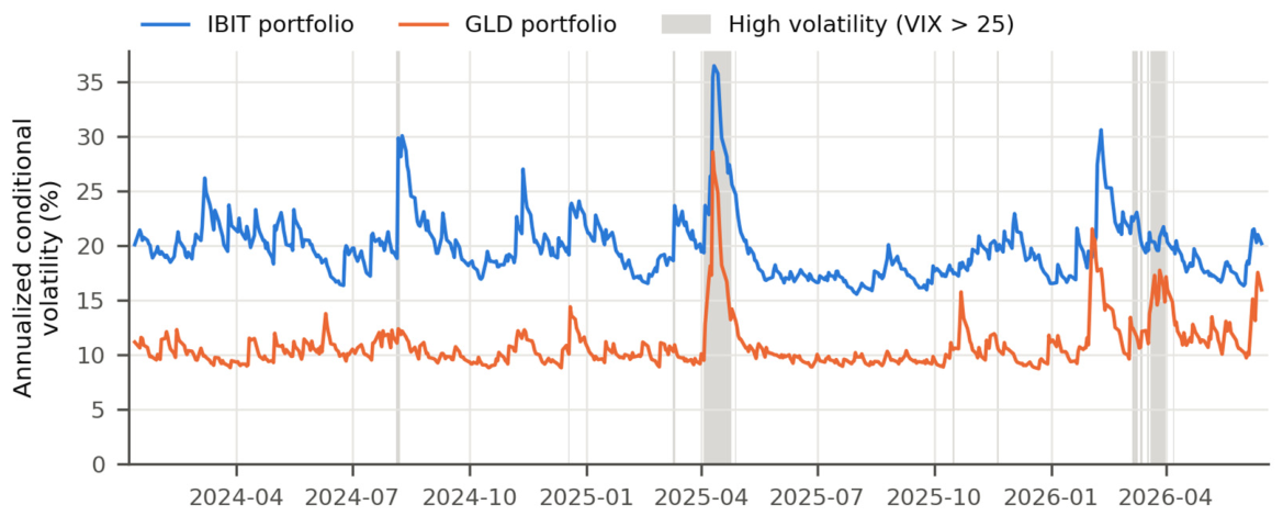
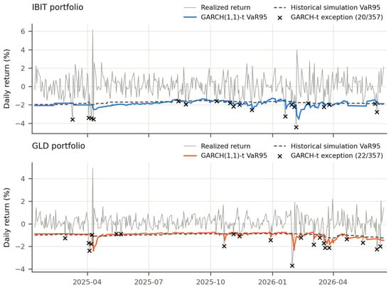
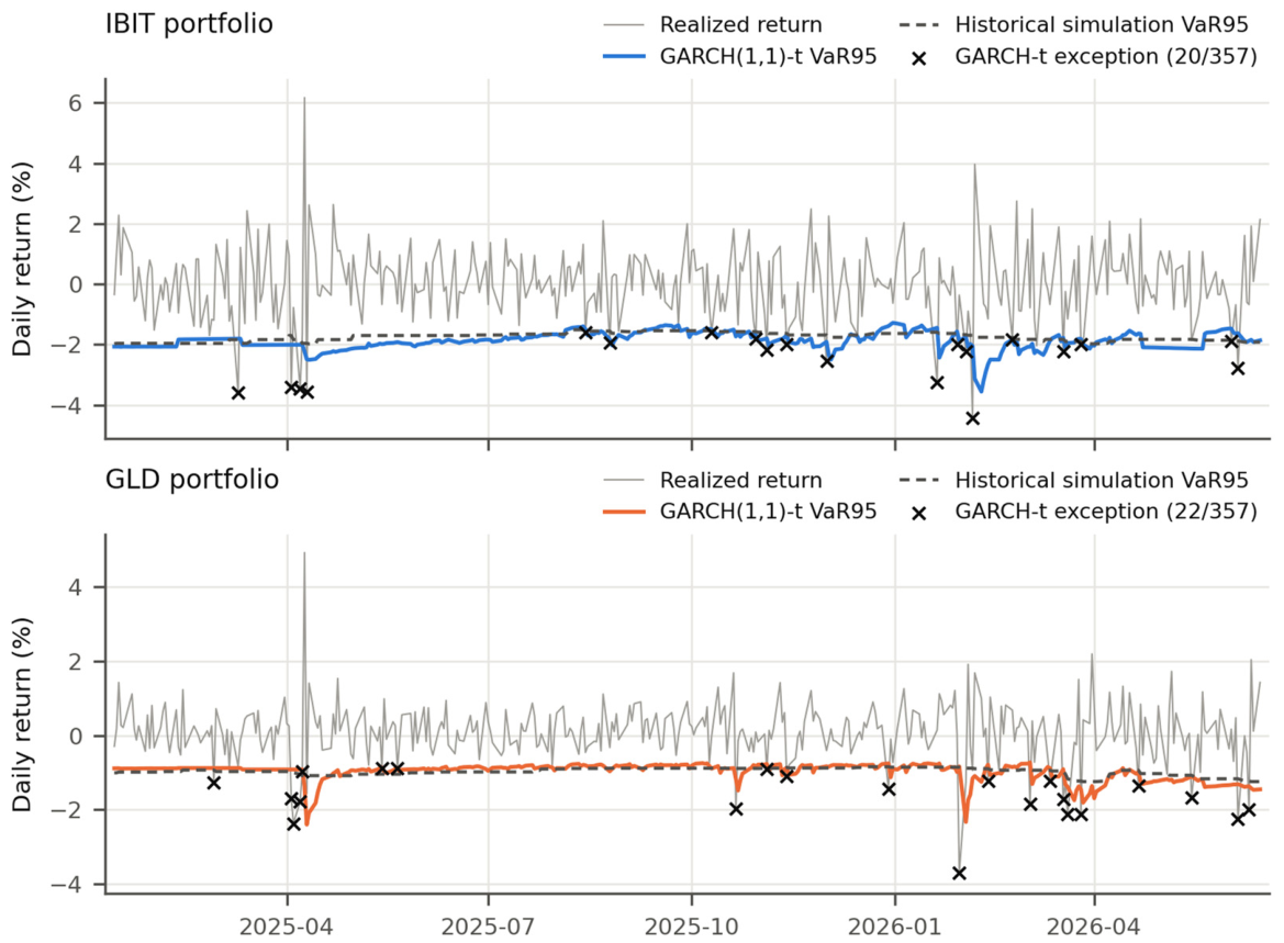
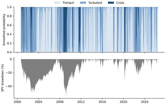
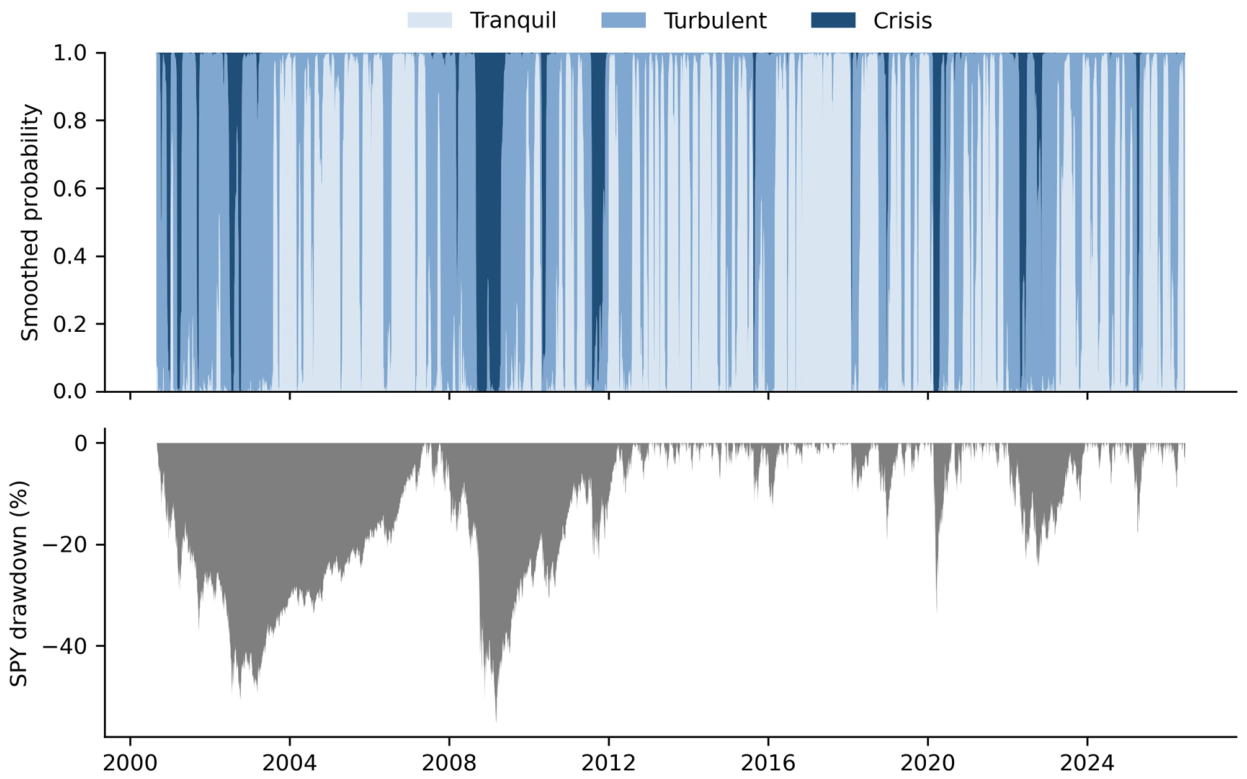
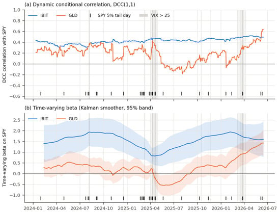
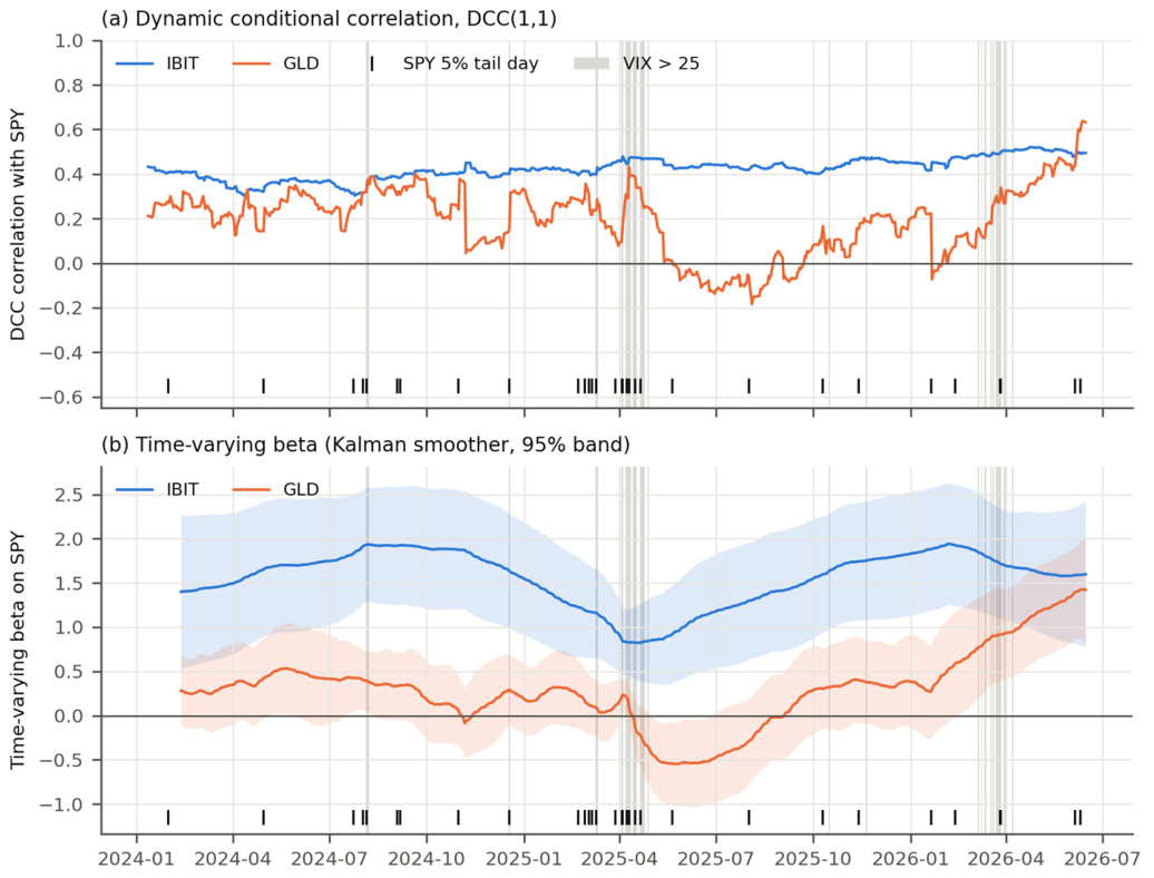

Disclaimer/Publisher’s Note: The statements, opinions and data contained in all publications are solely those of the individual author(s) and contributor(s) and not of MDPI and/or the editor(s). MDPI and/or the editor(s) disclaim responsibility for any injury to people or property resulting from any ideas, methods, instructions or products referred to in the content. |
© 2026 by the authors. Licensee MDPI, Basel, Switzerland. This article is an open access article distributed under the terms and conditions of the Creative Commons Attribution (CC BY) license.