


Abstract
Analyst consensus forecasts are widely used in investment decisions and as proxies for market expectations, yet they typically assign equal weight to component forecasts despite predictable differences in quality. We develop a constrained machine-learning framework that predicts each forecast’s relative quality from 29 ex ante analyst, forecast, broker, firm, and consensus characteristics and converts those predictions into positive, normalized weights. Over 21 sequential out-of-sample test years (2005–2025), the quality-weighted consensus reduces the late-horizon mean absolute error by 11.5% relative to the conventional mean and outperforms it in 62.9% of firm-years and every test year. Features locating a forecast within the contemporaneous distribution provide the largest incremental signal, while analyst track records, revisions, and broker attributes add further information. Improvements are larger when analyst coverage and forecast dispersion are high. The results show that forecast quality is inherently relative and that constrained machine learning can materially improve the consensus forecast accuracy by assigning context-dependent weights to individual forecasts based on their characteristics and the composition of the forecast set.
Keywords:
analyst forecasts; consensus forecasts; forecast aggregation; machine learning; expert weighting; earnings expectations JEL Classifications:
C53; G17; G24; M41
1. Introduction
Analyst consensus forecasts are central to investment decisions, corporate communication, and empirical research. Yet the standard consensus is usually a simple average that assigns the same weight to every forecast. It treats recent and stale forecasts, analysts with strong and weak records, and forecasts near the center and in the tails as equally informative. The consensus is therefore not a neutral statistic; it is an aggregation rule whose design can materially affect measured earnings expectations.
Equal weighting overlooks extensive evidence that forecast accuracy varies with firm-specific and general experience, brokerage resources, portfolio complexity, forecast frequency, prior accuracy, and forecast boldness (Mikhail et al., 1997; Clement, 1999; Jacob et al., 1999; Brown, 2001; Clement & Tse, 2003). The relevance of these characteristics also changes with the information environment. Disclosure regulation, media competition, and differences in information processing alter which analysts and forecasts are most informative (Keskek et al., 2017; Cao et al., 2022; Drake et al., 2024). Observable ex ante characteristics therefore contain quality signals, but their effects need not be linear or constant across firms, periods, and analyst sets.
Unequal weighting is not automatically superior. Averaging cancels idiosyncratic errors, measured analyst skill is noisy, forecast errors are correlated, and historically optimized weights can be unstable. These forces underlie the forecast combination puzzle: theoretically optimal or estimated weights often fail to outperform the simple average out of sample (Bates & Granger, 1969; Clemen, 1989; Stock & Watson, 2004; Timmermann, 2006; Genre et al., 2013). A useful method must therefore exploit predictable heterogeneity without surrendering the diversification benefit that makes the consensus difficult to beat.
The opportunity is economically important because consensus errors are predictable, and the consensus is widely used as a proxy for expected earnings. Analyst forecasts reflect bias, incentives, and incomplete information processing (Richardson et al., 2004; Keskek & Tse, 2018; Ham et al., 2022). Time-series and automated forecasts can outperform analysts in identifiable settings or add information when combined with them (Bradshaw et al., 2012; Ball & Ghysels, 2018), and predictable error adjustments improve valuation inputs and measures of earnings expectations (Mohanram & Gode, 2013; Keskek et al., 2020; Keskek & Rees, 2022). Most of this literature improves expectations outside the analyst set and therefore does not address how heterogeneous analyst forecasts should be combined.
Only a few studies address that decision directly. Butler et al. (2007) use a small set of characteristics in linear and inverse-variance weighting schemes and document meaningful, largely in-sample improvements. Michaely et al. (2024) retain only a prior-accuracy-based high-quality subset; their first-moment gains are modest and depend on sufficient breadth, while their strongest results concern forecast dispersion. Chen and Palmon (2024) report that characteristics-based consensuses predict announcement and post-announcement returns, but return predictability does not isolate forecast accuracy. The literature has therefore not established that a broad, continuously weighted, characteristics-based consensus can generate large and persistent real-time accuracy gains.
The unresolved challenge is a quality–diversity tradeoff. Forecasts from analysts who appear less accurate ex ante may still improve the aggregate when their errors offset those of others, while a historically strong analyst may issue a stale or uninformative forecast in a particular firm-year. Quality is therefore not a permanent analyst label. It is an observation-specific assessment that depends on who issued the forecast, when it was issued, how it changed, and how it relates to competing opinions. This logic makes fixed rankings, binary exclusion rules, and universal trimming thresholds incomplete. A useful aggregation rule must learn which differences matter in each forecast set while restricting the resulting weights enough to avoid overfitting.
The key unit of analysis is therefore not the analyst in isolation but the analyst-set combination. An analyst with a strong past record may add little when that analyst’s forecast duplicates information already reflected in the center of the distribution; a historically weaker analyst may improve the aggregate when the forecast supplies an independent signal that offsets shared error. Likewise, a tail forecast can represent either valuable dissent or noise. The marginal value of a forecast thus depends jointly on its issuer, timing, revision path, and relation to the other forecasts. This conditionality explains why evidence that characteristics predict individual accuracy does not by itself establish a superior consensus. It also makes the problem a natural setting for constrained ensemble learning: the model must assess relative contribution within a changing set rather than simply rank experts one at a time.
This tension motivates our central question: Can an adaptive but constrained weighting rule use ex ante analyst and forecast characteristics to improve the consensus consistently out of sample? A compelling answer requires more than a statistically significant average gain. The method should outperform the conventional equal-weighted consensus and relevant alternative weighting approaches, work across multiple forecast horizons and market regimes, preserve meaningful breadth in the analyst set, and reveal the conditions and mechanisms underlying its performance. These requirements shape both our model and our evaluation.
Three features make this a difficult real-time prediction problem. First, the composition and size of the analyst set vary across firms and years, so a fixed-dimensional covariance-based solution is difficult to estimate and maintain. Second, the mapping from characteristics to accuracy is likely nonlinear: forecast age may matter more in a dispersed set, boldness may be informative only for analysts with a strong track record, and broker resources may matter differently across information environments. Third, forecast errors are heavy-tailed, making unconstrained optimization prone to chasing rare observations. Our design responds by separating flexible quality prediction from a deliberately restricted aggregation rule. The boosted model learns interactions, while positive, normalized softmax weights preserve diversification and prevent economically implausible negative weights or extreme extrapolation. This combination of flexibility and discipline is central to this paper’s contribution to research on decision-making and forecast aggregation.
We address this gap with a constrained machine-learning aggregation framework. A gradient-boosted tree model predicts the relative quality of each forecast from 29 ex ante variables motivated by prior research and fixed before the out-of-sample tests. These variables capture analyst track records, cross-firm performance, revision behavior, broker resources, forecast timing, firm predictability, the contemporaneous analyst set, and the forecast’s position within that set. This broad information set is grounded in prior research and specified before the out-of-sample evaluation. All accuracy-based inputs are constructed from prior periods, and current-year realized earnings do not enter the variables used to determine current-year forecast weights. A softmax transformation converts the predicted quality into positive weights that sum to one. Unlike binary analyst selection, the method retains every forecast, and changes influence continuously, preserving opportunities for error cancellation while allowing quality effects to vary nonlinearly with context.
Importantly, the framework does not replace analyst judgment with a direct machine forecast of earnings. Analysts remain the source of the primary signals; machine learning determines how those signals should be combined. This architecture allows the model to preserve private and interpretive information embedded in analyst forecasts that may not be available in financial statements or standard time-series inputs. It also produces an observable set of weights that can be examined, constrained, and implemented, rather than a single opaque earnings prediction. The approach therefore speaks to a broader class of organizational decisions in which expert opinions are valuable but heterogeneous, panels change over time, and the decision maker must balance expertise against the error-cancellation benefits of aggregation.
The empirical design is prospective. For each test year from 2005 through 2025, estimation, validation, and tuning use only information available before the test year. The final sample contains 4.51 million annual EPS forecasts for 16,596 tickers over 1990–2025. We evaluate three forecast horizons, namely, more than 180 days, 91–180 days, and 2–90 days before the earnings announcement, and compare the quality-weighted consensus with the conventional equal-weighted mean and alternative characteristics-based and machine-learning weighting models. The primary loss is the mean absolute error (MAE), which measures the average forecast miss and is less sensitive than the squared loss to a small number of extreme errors.
The quality-weighted consensus produces economically large and persistent gains throughout the forecast cycle. In the late horizon, covering forecasts issued 2–90 days before the earnings announcement, MAE falls from $0.2543 to $0.2250 per share, a reduction of $0.0293, or 11.5%, relative to the conventional mean. The weighted consensus is more accurate in 62.9% of firm-years and has a lower annual MAE in all 21 test years. Importantly, the gains are larger earlier in the forecast cycle: MAE declines by 23.3% in the early horizon and 14.3% in the intermediate horizon. This pattern suggests that adaptive weighting is most valuable when uncertainty and differences in analyst information are greater, with the benefits diminishing as analysts incorporate more common information and forecasts therefore converge closer to the announcement.
The analysis also sheds light on the source of the improvement. Removing variables that locate a forecast within the contemporaneous distribution substantially reduces the late-horizon gain, although the interaction among feature blocks prevents an additive decomposition of their contributions. The evidence therefore points to observation-specific aggregation as an important source of the improvement: the model evaluates a forecast relative to the contemporaneous analyst set while using analyst histories, revisions, broker characteristics, and firm conditions as additional conditioning information. Consistent with this interpretation, the gains are larger when analyst coverage and forecast dispersion are high, settings in which the aggregation problem is more consequential.
The economic interpretation is important. The improvement is measured under absolute rather than squared loss, so it reflects a broad reduction in forecast misses rather than a few avoided extremes. This gives the findings relevance beyond analysts: many organizational and market decisions depend on combining changing panels of experts whose quality is observable only imperfectly and whose disagreements may contain either information or noise. The persistence of the gains across 21 test years further distinguishes the evidence from an isolated in-sample fit or a result driven by one market regime. Taken together, the findings indicate that the design of the aggregation rule is a first-order determinant of consensus quality rather than a minor technical choice.
This paper makes four contributions. First, it advances research on expert aggregation by showing that positive, normalized weights can preserve the wisdom of crowds while a nonlinear quality model exploits predictable differences in expertise. Second, it extends the analyst literature from explaining individual accuracy to improving the aggregate forecast itself. Relative to Butler et al. (2007), the design uses a broader information set, permits nonlinear and context-dependent effects, imposes stable positive weights, and evaluates performance over 21 sequential out-of-sample years. Relative to Michaely et al. (2024), it replaces binary selection with continuous weighting that preserves information from all component forecasts. Relative to Chen and Palmon (2024), it evaluates realized forecast accuracy directly rather than inferring forecast quality from return predictability.
Third, this paper contributes to machine-learning forecasting by improving the aggregation rule rather than replacing expert forecasts with a direct black-box prediction of earnings. The results show that much of the value comes from learning the geometry of the contemporaneous forecast distribution and conditioning the treatment of its tails on analyst and firm information. Finally, this paper contributes to market-expectation research and practice. A more accurate consensus can reduce measurement error in studies of earnings news, earnings-response coefficients, and post-earnings-announcement drift, while providing forecast users with an implementable alternative to conventional equal weighting and binary analyst-selection rules.
2. Related Literature and Incremental Contribution
2.1. Consensus Forecasts, Predictable Errors, and Alternative Expectations
The usefulness of the analyst consensus depends on how component forecasts are selected and combined. O’Brien (1988) shows that the choice of forecasts affects the quality of the expectations proxy, and Brown (1991) finds that recency-based selection can improve accuracy. Kim et al. (2001) show that the mean can inefficiently summarize forecasts that share public information, while Markov and Tamayo (2006) document predictable structure in analyst errors. These studies establish that consensus construction is an empirical choice rather than a mechanical convention and motivate examining whether the standard equal-weighting rule can be improved.
A related strand of literature identifies predictable errors within analyst forecasts. Forecast walk-downs reflect managerial and analyst incentives (Richardson et al., 2004), bias affects market influence (Keskek & Tse, 2018), and analysts incompletely incorporate firm-specific and industry information (Keskek & Tse, 2024). Analysts also communicate information without revising numerical forecasts (Berger et al., 2019), and cross-horizon forecasts predict more than 10% of the subsequent forecast error (Ham et al., 2022). Drake et al. (2024) further show that forecasts differ in their informational origins. The forecasts entering a consensus are therefore heterogeneous in both expected accuracy and information content, providing a basis for assigning them different ex ante weights.
Statistical forecasts provide complementary evidence. Analyst superiority over time-series forecasts is conditional (Bradshaw et al., 2012), and automated forecasts can add information to analyst estimates (Ball & Ghysels, 2018). Alternative or adjusted expectations measures also capture information omitted by the conventional consensus (Livnat & Mendenhall, 2006; Mohanram & Gode, 2013; Keskek & Rees, 2022). These studies establish that expected-earnings measures can be improved, but they generally replace or adjust the analyst consensus using information outside the analyst set. Our objective is different: analyst forecasts remain the primary signals, and the decision is how to aggregate them. A better aggregation rule can therefore improve the earnings-expectations proxy without discarding analysts’ private and interpretive information.
2.2. Analyst Heterogeneity and Prior Aggregation Approaches
Research on individual analysts provides a rich set of candidate quality signals. Accuracy varies with firm-specific experience, general experience, brokerage resources, portfolio complexity, forecast frequency, prior accuracy, reputation, and forecast boldness (Mikhail et al., 1997; Clement, 1999; Jacob et al., 1999; Stickel, 1992; Brown, 2001; Clement & Tse, 2003). The relevance of these attributes changes with disclosure rules and external information supply (Keskek et al., 2017; Cao et al., 2022). This evidence motivates a conditional weighting model: observable analyst and forecast characteristics contain information about expected accuracy, but the same characteristic need not imply the same forecast quality across firms, periods, or information environments.
Early aggregation studies use relatively simple rules. Brown and Mohd (2003) rank forecasts on selected characteristics and impose an ad hoc declining weight schedule. Butler et al. (2007) provide the closest systematic framework. Their variance–covariance approach predicts forecast-error variance from age, frequency, broker size, and experience and applies inverse-variance weights; their regression approach estimates linear adjustments to the mean. They report MSE improvements of roughly 3–15%, depending on the number of forecasts. The gains are concentrated in high-dispersion observations and arise mainly from forecast age and frequency.
Butler et al. (2007) establish that analyst and forecast attributes can improve aggregation, but their design leaves the central implementation problem unresolved. Their predictor set is limited, characteristic effects are linear or embedded in simplified covariance assumptions, and the principal tests use the historical sample on which the weighting relations are estimated. The authors explicitly identify estimation error and real-time out-of-sample performance as open questions. Their more comparable inverse-variance tests reduce the absolute error by about 4.3% for a 60-day window and 6.8% for a 180-day window. Our 11.5% late-horizon improvement is not a formal horse race because samples, horizons, and methods differ; it motivates a broader adaptive design and a long sequential out-of-sample evaluation.
Michaely et al. (2024) offer a complementary benchmark. They rank analysts using prior-year firm-specific accuracy and compare the equal-weighted average of the high-quality subset with the full consensus. The classification is ex ante for the test-year forecast, but the aggregation rule is discrete: lower-ranked analysts receive zero weight, and selected analysts receive equal weight. Because exclusion sacrifices potential error cancellation, the high-quality subset outperforms the full consensus only when the subset contains sufficient breadth, and the first-moment improvement is modest. Their strongest results concern the information in high-quality analyst dispersion. Our approach instead retains all forecasts and varies their influence continuously, allowing predicted quality to matter without imposing a binary cutoff.
Chen and Palmon (2024) revisit characteristics-based consensus forecasts using quarterly U.S. data. Their published abstract reports that alternative consensuses predict announcement-window and post-announcement abnormal returns better than the simple mean and, in some tests, the median. However, return predictability can reflect forecast accuracy, the expectation investors use, risk, or mispricing, and therefore does not isolate the aggregation objective. We instead evaluate the realized forecast error directly and compare the proposed rule with the conventional equal-weighted consensus and alternative characteristics-based and machine-learning weighting approaches. This design isolates whether analyst heterogeneity can be used to improve the accuracy of the consensus itself, rather than whether an alternative consensus contains information associated with subsequent returns.
2.3. Forecast Combination and Machine Learning
The classic forecast combination result assigns weights using the inverse forecast-error covariance matrix (Bates & Granger, 1969). In practice, the analyst set changes across firms and years, error covariances are imprecisely estimated, and structural change can make historical weights unstable. Reviews by Clemen (1989) and Timmermann (2006), together with evidence from Stock and Watson (2004) and Genre et al. (2013), explain why the equal-weighted average remains a demanding benchmark. A successful method must therefore exploit predictable differences in forecast quality while constraining the resulting weights sufficiently to remain stable out of sample.
Gradient-boosted trees are well suited to this setting because they accommodate nonlinearities, thresholds, and interactions without estimating a separate forecast-error covariance matrix for each changing analyst set. Machine learning has improved prediction in finance and accounting (Gu et al., 2020; Hunt et al., 2019), and LightGBM provides a scalable implementation of gradient boosting (Ke et al., 2017). Our use of machine learning differs from direct earnings-prediction applications: the model predicts the relative quality of the component forecasts, while a constrained aggregation layer determines their influence. This separation preserves the information contained in analyst judgments while allowing the aggregation rule to adapt to the composition of each forecast set.
2.4. Incremental Contribution
Taken together, the closest studies show that analyst heterogeneity can matter for consensus information, but they do not provide a broadly applicable, real-time solution to the aggregation problem. Butler et al. (2007) use a relatively limited characteristic set and linear or covariance-based weighting structures; Michaely et al. (2024) use binary analyst selection and document limited first-moment improvements; and Chen and Palmon (2024) focus primarily on the return implications of characteristics-based consensuses rather than realized forecast accuracy. We extend this literature by combining a broad ex ante information set with nonlinear, context-dependent quality prediction, continuous positive weighting, and a 21-year sequential out-of-sample evaluation.
The contribution also extends beyond identifying better analysts. Our framework jointly evaluates who made a forecast, how the forecast evolved, and where it lies within the current distribution of opinions. Forecast quality is therefore treated as observation-specific rather than as a fixed analyst attribute. This structure allows the aggregation rule to exploit analyst heterogeneity while retaining the diversification benefits of the full forecast set. More broadly, the framework illustrates how constrained machine learning can improve collective prediction when expert quality is heterogeneous, context-dependent, and only imperfectly observable. For accounting and finance research, the resulting consensus provides a potentially more accurate expected-earnings benchmark for studying earnings news, market reactions, and related capital-market outcomes.
3. Data and Sample
3.1. Data Sources and Sample Filters
The primary data source is the I/B/E/S Detail History file, which provides individual analyst EPS forecasts, analyst and broker identifiers, forecast dates, fiscal-period-end dates, and reported actual earnings. We focus on annual EPS forecasts for U.S. firms and merge the forecast data with Compustat Fundamentals Annual variables that characterize the firm’s historical earnings environment.
To track individual analysts longitudinally across time and across brokerage houses, we rely on the permanent analyst identification code (ANALYS) in I/B/E/S, while brokerage houses are identified by the ESTIMATOR code. Tracking forecasters via their permanent ANALYS identifier ensures that an analyst’s historical track record (e.g., firm-specific tenure, prior forecasting errors, and cumulative career breadth) is preserved even when an analyst switches employers. When an analyst moves to a new brokerage house, broker-level attributes (such as broker size and broker historical accuracy) update to reflect the new employer, while individual experience metrics continue to accumulate. If an analyst begins covering a firm for the first time or resumes coverage after an interruption, firm-specific lagged accuracy measures may be unavailable. We retain these observations and leave the corresponding lagged variables missing rather than imposing arbitrary values. Section 4 describes how the prediction model accommodates missing features.
Forecasts must be issued at least two calendar days before the earnings announcement date (EAD) and no more than 365 days before the announcement. We exclude observations with absolute reported EPS exceeding $50, absolute forecasted EPS exceeding $100, analysts associated with more than 100 tickers in a single calendar year, and firm-years with fewer than three distinct active analysts. The 100-ticker restriction serves as a standard data-cleaning filter to remove programmatic algorithmic feeds rather than individual human forecasters. For each analyst–firm–year–horizon, we retain the analyst’s most recent forecast within the corresponding horizon window. The final sample contains 4,508,469 forecast-level observations covering 16,596 tickers from 1990 through 2025.
3.2. Forecast Horizons and Evaluation Units
Forecast horizon is measured as the number of calendar days between the analyst’s forecast announcement date and the firm’s earnings announcement date. We define three distinct evaluation horizons based on forecast timeliness: the early horizon evaluates forecasts outstanding more than 180 days before the earnings announcement, the intermediate horizon evaluates forecasts outstanding 91–180 days before the announcement, and the late horizon evaluates forecasts outstanding 2–90 days before the announcement. Anchoring the horizon windows to the earnings announcement date provides a standardized framework for evaluating forecast quality as information accumulates across the fiscal cycle.
For analyst i, firm j, and year t, the forecast horizon is defined as:
where is the calendar date of firm j’s actual earnings announcement for fiscal year t and is the date analyst i issued or revised the forecast. Importantly, our empirical evaluation protocol is defined separately for each forecast-horizon window. For each firm–year–horizon, we restrict the forecast set to estimates issued within the corresponding window and retain each analyst’s most recent forecast within that window. For example, in the late horizon, we consider forecasts issued from 2 to 90 calendar days before the earnings announcement date (EAD) and retain the most recent forecast issued by each analyst during that period. Forecasts issued more than 90 days before the announcement or within the final day before the announcement are excluded from the late-horizon evaluation. All consensus-position and analyst-set variables—including the forecast percentile, distance from the consensus, consensus dispersion, range, skewness, and coverage—are then calculated from this resulting cross-sectional set of retained forecasts. Because all forecasts and contemporaneous consensus characteristics are constructed prior to the earnings announcement, realized current-year earnings are unobserved when forecast quality is assessed and therefore do not enter the weighting process.
The unit of evaluation is the firm–year–horizon. Within each unit, analyst coverage is the number of distinct analysts contributing forecasts to that horizon, so coverage can vary for the same firm across years and horizons as analysts initiate or discontinue coverage. The conventional consensus benchmark is the equal-weighted mean of the retained analyst forecasts. The sequential out-of-sample evaluation begins in 2005, leaving 1990–2004 to construct historical analyst characteristics and determine model specifications before the test period begins.
3.3. Overall Research Framework and Empirical Architecture
To provide an integrated overview of the research design, Figure 1 shows the logical progression across the five sequential stages of our empirical framework. For each stage, the diagram maps the specific inputs, analytical processes, intermediate and terminal outputs, and corresponding research objectives.
Figure 1.
Research design architecture: input–process–output–objective framework.
Stage 1 links individual forecast records from I/B/E/S Detail History with Compustat accounting fundamentals, using permanent analyst identifiers (ANALYS) to track careers across brokerage transitions while partitioning forecasts into three standardized horizons (early, intermediate, and late). Stage 2 constructs 29 observable characteristics across nine economic dimensions strictly prior to the earnings announcement, alongside the bounded relative forecast quality target. Stage 3 implements an expanding walk-forward LightGBM architecture with Huber loss, native split-routing for missing values, and temporal cross-validation to prevent forward-looking data leakage. Stage 4 transforms raw predicted quality scores into strictly positive, convex weights via softmax, computing the quality-weighted consensus forecast. Finally, Stage 5 benchmarks the quality-weighted consensus against equal-weighted mean consensus measures across 21 out-of-sample years (2005–2025) using Diebold–Mariano tests and Fama–MacBeth cross-sectional regressions.
4. Research Design
4.1. The Aggregation Problem
Let denote the earnings per share forecast issued by analyst i for firm j in fiscal year t, and let Njt is the total number of analysts covering firm j in year t. The conventional consensus assigns an equal weight of to every forecaster:
Our objective is to replace the uniform weights with forecast-specific weights, , that reflect the predicted relative forecast quality, are non-negative, sum to one, and depend only on information available when the consensus is formed for the relevant forecast horizon (ex ante observability). Positivity and normalization preserve diversification and prevent extreme extrapolation; forecast-specific variation permits more informative opinions to receive greater influence on the consensus. These restrictions are substantive, not merely computational: an individually less accurate forecast can still offset errors in other forecasts, so discarding analysts or concentrating on a single apparent winner can reduce group accuracy.
This approach reconciles expertise weighting with the wisdom of crowds. Binary selection requires analyst quality to be sufficiently persistent and the selected subset to be large enough to retain diversification, conditions that help explain the mixed first-moment evidence in Michaely et al. (2024). Continuous weights instead make predicted quality consequential without imposing a sharp cutoff. Every forecast remains in the combination, but its influence changes with the strength of the ex ante quality signal.
We implement our empirical framework through a sequential multi-stage procedure. We begin by ingesting raw forecast records from the I/B/E/S Detail History file and fundamental accounting data from Compustat and apply the sample filters described in Section 3. For each firm–year–horizon, we restrict forecasts to the corresponding horizon window and retain each analyst’s most recent forecast within that window. We then construct the complete set of 29 ex ante characteristics from historical analyst information and the contemporaneous cross-section of retained forecasts.
Using historical observations, we convert the realized forecast accuracy into a rank-normalized relative quality target, . We then estimate a LightGBM gradient-boosted tree ensemble using an expanding-window walk-forward design. For each test year from 2005 through 2025, the LightGBM model is estimated exclusively on observations from years preceding .
We then apply the fitted model to test year t to generate out-of-sample predicted quality scores, , for all active analysts covering the firm. Through the softmax transformation with concentration parameter , we map these predicted quality scores into strictly positive, normalized weights, , that sum to one. Finally, we compute the quality-weighted consensus, , and evaluate its out-of-sample performance against realized actual earnings across 21 sequential test years (2005–2025) using the mean absolute error, loss differentials, observation win rates, and out-of-sample . This procedure is repeated sequentially for each of the 21 out-of-sample test years from 2005 through 2025.
4.2. Ex Ante Feature Set
The model uses 29 ex ante variables organized into nine information blocks. The feature set is grounded in constructs emphasized in prior research on analyst accuracy, experience, forecasting behavior, brokerage resources, and the information environment. Some variables closely follow measures used in prior studies, while others extend these constructs to capture additional dimensions of forecast history or relative position within the contemporaneous analyst set. The complete information set was specified before evaluating the performance over the 2005–2025 out-of-sample period.
Analyst-history variables include lagged firm-specific errors, their mean, variability, and trend. Cross-firm performance captures prior accuracy across the analyst’s portfolio and the frequency with which the analyst ranks in the more accurate half of a forecast set. These variables distinguish persistent skill from a one-time firm-specific outcome, building on evidence of analyst forecasting ability and learning (e.g., Mikhail et al., 1997; Clement, 1999). Experience and workload variables measure the analyst’s tenure covering the firm, cumulative forecasting experience, and the number of firms covered in the current year, capturing firm-specific learning, general expertise, and portfolio complexity (e.g., Clement, 1999; Jacob et al., 1999; Brown & Mohd, 2003).
The remaining blocks describe the forecast and its environment. Consensus-position variables measure the standardized distance from the mean, percentile rank, direction relative to the mean, and tail status, capturing bold versus herding behavior (e.g., Clement & Tse, 2005). Revision variables capture frequency, magnitude, and direction. Broker variables capture resources and prior broker performance; firm variables capture lagged earnings volatility and prior consensus surprise; and analyst-set variables capture dispersion, range, skewness, and coverage, controlling for task complexity and disagreement (e.g., Butler et al., 2007). Forecast horizon and related timing controls complete the feature set. The representation therefore captures both forecaster attributes and the geometry of the current forecast distribution, allowing the same analyst and the same degree of forecast boldness to receive different weights across firms, years, and information environments.
All accuracy-based variables are constructed using information from prior periods only. Analyst-varying characteristics are rank-normalized within the firm–year–horizon when appropriate, allowing the model to learn relative quality within the set being aggregated. No current-year realized earnings are used to construct the features that determine current-year forecast weights.
4.3. Quality Prediction Model
Within each firm–year–horizon, realized absolute errors are converted into a rank-based quality target, with higher values assigned to more accurate forecasts. Let xijt denote the vector of ex ante characteristics associated with analyst i’s forecast for firm j in year t, and let qijt denote the corresponding rank-normalized quality target, scaled to [0, 1] such that higher values indicate greater accuracy (lower forecast error). We estimate:
where g(.) is a LightGBM gradient-boosted tree ensemble (Ke et al., 2017). Trees capture thresholds and interactions such as whether a distant forecast is more informative when dispersion is high, coverage is broad, or the analyst has a strong prior record. This flexibility allows the model to treat the same forecast position differently depending on the surrounding analyst set and other observable characteristics. For example, a forecast far from the consensus may be less informative in a tightly clustered analyst set but potentially more informative when dispersion is high, coverage is broad, or the analyst has a strong prior record. Thus, an extreme forecast need not receive the same treatment across firms, years, or information environments.
qijt = g(xijt) + εijt
The implementation uses a learning rate of 0.05, up to 300 trees with early stopping, maximum depth of six, minimum leaf size of 100, row subsampling of 80%, column subsampling of 70%, and L1 and L2 regularization. All hyperparameters were tuned via cross-validation conducted exclusively over the 1990–2004 pre-sample validation period prior to out-of-sample testing, with early stopping triggered if validation loss failed to improve for 30 consecutive rounds. Missing feature values are handled natively through LightGBM’s optimal split-routing algorithm, avoiding arbitrary imputation distortions. As reported later, the quality model retains substantial explanatory power out of sample; together with the sequential walk-forward results, this provides evidence that the estimated relations generalize beyond the estimation sample.
4.4. From Quality Scores to Consensus Weights
Predicted quality scores, are converted into positive, normalized consensus weights using a softmax transformation:
where is the out-of-sample predicted relative accuracy of analyst i’s forecast, and the denominator sums over all active analysts covering firm j in year t. The concentration parameter, controls the degree of departure from equal weighting. When gamma equals zero, the exponential terms equal one, and every analyst receives an equal weight of , recovering the conventional consensus mean. Larger values of gamma assign progressively greater weight to analysts with higher predicted quality while exponentially downweighting lower-quality forecasts. In the limit as , the weighting converges to a winner-take-all selection of the single highest-ranked analyst.
The transformation separates flexible quality prediction from a tightly constrained aggregation rule: the boosted-tree model captures complex nonlinearities and interaction effects in analyst quality, while the softmax layer restricts weights to a valid convex combination, ruling out negative, extreme, or non-normalized values. The resulting quality-weighted consensus forecast is defined as:
where fijt denotes the most recent annual EPS forecast issued by analyst i for firm j in fiscal year t within the designated horizon window, is the estimated quality weight assigned to that forecast from the softmax layer (satisfying and ), and is the total number of distinct analysts covering firm j in year t. Because every weight is strictly positive and bounded, the aggregation rule retains all component forecasts and preserves the scope for error diversification while shifting greater influence toward forecasts with higher predicted quality.
This structure regularizes the changing-set combination problem. Butler et al. (2007) estimate weights from a small characteristic set under linear or simplified covariance structures and identify estimation error as a central obstacle to real-time implementation. We avoid estimating a separate forecast-error covariance matrix for each firm-year analyst set. Positive normalized weights limit instability, while the quality model uses a common nonlinear mapping learned across analyst sets.
In our primary specification, we set gamma = 10 based on the pre-test validation period. At this value, the effective number of contributing analysts, defined as , averages 4.3 in the late horizon with an average maximum weight of 0.38, indicating that the consensus continues to place meaningful weight on multiple forecasts rather than collapsing to a single predicted winner.
4.5. Walk-Forward Evaluation and Loss Functions
We use an expanding-window walk-forward design. For each test year t from 2005 through 2025, model estimation, early stopping, and parameter selection rely only on observations available before year t. The resulting fitted model is then applied to year t without using test-year outcomes. This procedure mirrors the information set of a real-time forecast user and directly addresses the out-of-sample limitation identified by Butler et al. (2007).
Our primary measure of forecast accuracy is the mean absolute error (MAE) computed across all firm-year observations in the out-of-sample test period:
where is the realized annual earnings per share reported by firm j for fiscal year t, is the consensus forecast generated under a given aggregation method for firm j in year t, and |T| is the total number of firm-year observations in the evaluation sample T. Absolute loss is less dominated than squared loss by a small number of extreme forecast errors and has a direct interpretation as the average forecast miss.
To evaluate whether the quality-weighted consensus delivers statistically significant accuracy gains over the conventional benchmark, we compute the firm-year loss differential:
where is the conventional equal-weighted mean forecast, and is our quality-weighted consensus forecast. Hence, djt represents the per-share absolute error reduction achieved by quality weighting for firm j in year t; positive values (djt > 0) indicate that the quality-weighted consensus is strictly closer to realized earnings than the equal-weighted mean. The reported loss-difference t-statistics follow the Fama and MacBeth (1973) procedure: for each of the 21 test years (2005–2025), we compute the cross-sectional mean loss differential, across all firms in year t () and then test whether the time-series mean of these 21 annual averages differs significantly from zero. This approach clusters standard errors by calendar year and is robust to cross-sectional correlation among firms within the same year.
djt = |Meanjt − Actualjt| − |Weightedjt − Actualjt|
We also report two complementary measures of out-of-sample performance. First, the observation win rate is the percentage of firm-year observations for which the quality-weighted consensus is strictly closer to realized earnings than the conventional equal-weighted mean.
where is the absolute error differential, is the indicator function taking the value 1 when the quality-weighted consensus is strictly more accurate than the benchmark and 0 otherwise, and is the total number of evaluated firm-year observations.
A win rate above 50% indicates that the improvement extends to a majority of observations rather than being driven by a small number of unusually large forecast errors.
Second, following Campbell and Thompson (2008), we measure the proportional mean squared error reduction relative to the equal-weighted mean defined as:
where is the conventional equal-weighted mean consensus forecast (the standard benchmark), is the quality-weighted consensus forecast, is the realized actual earnings, is the total squared forecast error of the quality-weighted consensus, and is the total squared forecast error of the conventional equal-weighted consensus. A positive value indicates that the quality-weighted consensus delivers lower mean squared error than the conventional consensus.
5. Results
Table 1 reports the sample selection. The full dataset contains 4,508,469 individual annual EPS forecasts covering 16,596 unique tickers from 1990 through 2025. Forecasts are classified into three horizons based on their distance from the earnings announcement date: the sample contains 95,765 early-horizon firm-years, 118,192 intermediate-horizon firm-years, and 112,611 late-horizon firm-years. The sequential out-of-sample evaluation covers 2005–2025, providing 21 test years, and each firm–year–horizon is required to contain forecasts from at least three distinct analysts.
Table 1.
Sample summary.
Table 2 reports the summary statistics for the forecast-accuracy target and all model characteristics, while Appendix A provides variable definitions and construction details. The mean absolute individual forecast error is $0.401 per share, compared with a median of only $0.070. The large difference between the mean and median, together with a standard deviation of $1.975, indicates that forecast errors are strongly right-skewed and contain relatively large tail observations. This distribution supports the use of the mean absolute error as the primary evaluation criterion because absolute loss is less sensitive than squared loss to unusually large forecast errors. The average forecast horizon is 93 days, while the median is 63 days. Analyst coverage averages 14.88 forecasts per firm–year–horizon, with an interquartile range from 7 to 21 analysts, indicating meaningful variation in the breadth of the analyst set.
Table 2.
Summary statistics.
The characteristics used to predict forecast quality also exhibit considerable heterogeneity. Prior-year forecast error averages $0.247, while the average track record error is $0.245. Analysts issue an average of 3.76 revisions, and revision magnitude has a mean of $0.539 but a median of only $0.100, again indicating substantial right skewness. Consensus dispersion averages $0.343, compared with a median of $0.088, and the average consensus range is $1.112 compared with a median of $0.290.
Finally, the variation in analyst experience, firm conditions, and forecast-set characteristics provides substantial information for the model to exploit. Analysts have an average firm-specific tenure of 2.84 years, career breadth of 111.4 firm-year assignments, and coverage breadth of 17.02 firms. Earnings volatility and prior-year surprise also display substantial dispersion. Overall, the summary statistics document substantial heterogeneity in forecast accuracy, analyst characteristics, and the contemporaneous information environment, providing empirical motivation for allowing forecast weights to vary across analysts and forecast sets rather than imposing equal weights universally.
5.1. Main Out-of-Sample Accuracy
Table 3 reports the main out-of-sample results. We clarify the distinction between the sample counts reported in Table 1 and Table 3. Table 1 describes the full historical data archive spanning 36 calendar years (1990–2025), encompassing both the 15-year initial training period (1990–2004) and all firm-years before horizon-specific coverage filters. In contrast, Table 3 evaluates out-of-sample performance strictly for the 21-year test period (2005–2025) and restricts observations to firm-years with at least three distinct analysts issuing forecasts within that specific horizon window. Because early-horizon forecasts require early analyst coverage, the active out-of-sample firm-year count meeting the multi-analyst filter (≥3 active analysts strictly within the horizon window) is naturally smaller in the early horizon (5626 firm-years) and intermediate horizon (21,120 firm-years) than in the broader test archive. For the late horizon, although 58,416 total firm-years are available across the 2005–2025 out-of-sample period prior to horizon-specific coverage restrictions, requiring at least three distinct analysts issuing active forecasts strictly within the 2–90 day pre-announcement window and possessing complete historical features yields the primary evaluated test sample of 16,933 multi-analyst firm-years reported in Table 3. The quality-weighted consensus is more accurate than the equal-weighted mean across all three horizons. Relative to the equal-weighted mean, the MAE declines by 23.3% in the early horizon, 14.3% in the intermediate horizon, and 11.5% in the late horizon. The weighted consensus also produces a lower aggregate MAE in every test year for each horizon. The pattern indicates that analyst and forecast characteristics contain useful information throughout the forecast cycle, with the largest proportional gains occurring when forecasts are issued further from the earnings announcement date. As the announcement date approaches, analysts incorporate more common information, and their forecasts converge, reducing the scope for improving on the conventional consensus. Even in the late horizon, however, the quality-weighted consensus continues to produce economically meaningful accuracy gains.
Table 3.
Quality-weighted consensus versus equal-weighted mean.
In the remainder of our analysis, we focus on the late horizon, although the results and inferences are generally consistent across all three forecast horizons. The quality-weighted consensus reduces the MAE from $0.2543 to $0.2250 per share, an absolute reduction of $0.0293 per share. This is an 11.5% improvement relative to the equal-weighted mean. Because performance is evaluated using absolute loss, not squared loss, the improvement is less likely to be driven disproportionately by a few extreme errors. The quality-weighted consensus has a lower absolute error than the equal-weighted mean in 62.9% of firm-year observations and a lower annual MAE in all 21 test years. Taken together, the aggregate MAE reduction, the broad observation-level win rate, and the consistency across test years indicate that the improvement is not concentrated in a small number of forecast errors or a particular subperiod.
To place the magnitude in context, the $0.0293 per-share reduction in the late-horizon MAE represents 11.5% of the conventional consensus MAE. The improvement is economically relevant for applications in which analyst consensus forecasts are used as proxies for expected earnings. In particular, a more accurate consensus may reduce measurement error in earnings surprises used in research on earnings-response coefficients, post-earnings-announcement drift, valuation, and related market-expectation tests.
5.2. What Generates the Improvement?
Table 4 examines the contribution of different feature sets and compares the full model with more parsimonious alternatives. The full 29-variable model reduces the late-horizon MAE by approximately 11.5%. Excluding the four consensus-position variables lowers the gain to 4.8%, while excluding all consensus variables lowers it to 3.3%. A specification based primarily on analyst track records and basic controls improves the MAE by 2.4%, while a seven-variable linear benchmark improves it by 1.0%. These results indicate that traditional analyst characteristics contain statistically and economically useful information but account for only a minority of the full model’s improvement. The much larger gain from the full model suggests that the aggregation quality depends not only on who the analyst is but also on how each forecast is positioned within the contemporaneous forecast set.
Table 4.
Feature-block and model comparisons: late horizon.
Table 4 also compares the full model with alternative econometric and machine-learning specifications estimated over the same walk-forward test period. The seven-variable linear model reduces the MAE by 1.0%, the full 29-variable linear model by 2.8%, and regularized linear models by 3.1%. The Set-Attention Transformer and direct-MAE neural-network specifications produce larger reductions of 6.6% and 7.1%, respectively, but remain below the 11.5% improvement from the full LightGBM model. An adaptive- LightGBM specification performs similarly, reducing the MAE by 11.2%. These comparisons indicate that the improvement reflects more than simply expanding the predictor set: allowing nonlinear and context-dependent relations while retaining a constrained aggregation rule contributes importantly to performance.
The model’s primary advantage therefore appears to arise from observation-specific aggregation rather than from identifying a fixed group of persistently superior analysts. The machine-learning rule conditions the forecast weights on the distribution of contemporaneous forecasts together with analyst history, revision behavior, broker information, and the firm’s earnings environment. Thus, an extreme forecast may receive little weight in a tight distribution when the analyst lacks supporting history, yet it may retain meaningful weight when dispersion is high, the analyst has a strong record, or firm conditions make a bold forecast more informative. Overall, the evidence supports the inference that the largest gains come from jointly evaluating forecast characteristics and their context rather than relying on analyst quality or any single characteristic in isolation.
5.3. Coverage and Forecast Dispersion
Table 5 examines the late-horizon performance across analyst-coverage groups. The economic benefit of quality weighting increases with the number of analysts contributing to the consensus. The MAE reduction rises from 10.6% for firms with three to five analysts to 29.7% for firms with more than twenty analysts; the corresponding win rate increases from 61.7% to 79.1%, respectively. Because the highest-coverage group contains relatively few observations, its magnitude should be interpreted cautiously. Nevertheless, the broader pattern indicates that adaptive weighting becomes more valuable as the forecast set expands. Larger analyst sets provide more potentially useful information and greater opportunities for error cancellation. The results therefore suggest that the model makes more effective use of cross-sectional heterogeneity than the conventional equal-weighting rule.
Table 5.
Accuracy by analyst coverage: late horizon.
Table 6 examines the performance across terciles of forecast dispersion. The MAE improvement is approximately 4.3% in the bottom tercile, 5.0% in the middle tercile, and 13.6% in the top tercile. When analyst forecasts are tightly clustered, alternative positive weighting schemes produce similar aggregates, leaving relatively little scope for improvement. As disagreement increases, however, both the position and the source of each forecast become more consequential for aggregation. The substantially larger gains in the high-dispersion subsample are consistent with Butler et al. (2007), but here, they are obtained under absolute loss and a 21-year walk-forward design. Overall, the evidence suggests that adaptive weighting is particularly valuable when the aggregation problem is more complex, i.e., when many analysts contribute forecasts and when those forecasts differ substantially.
Table 6.
Accuracy by forecast dispersion: late horizon.
5.4. Feature Importance and Weight Concentration
Table 7 reports the leading variables based on LightGBM split importance in the late-horizon model, identifying which of the 29 literature-derived characteristics drive aggregation efficiency most significantly. The empirical contributions naturally divide into three distinct tiers:
Table 7.
Leading LightGBM feature-importance measures: late horizon.
First, consensus-position and distributional geometry variables emerge as the primary drivers of forecast efficiency, accounting for approximately 73% of the total MAE reduction (as documented in the ablation study in Table 4). Forecast percentile ranks first, followed by standardized consensus distance, consensus skewness, and consensus dispersion. These four variables allow the gradient-boosted trees to implement an adaptive nonlinear trimming mechanism: forecasters situated in the extreme tails (percentiles ≤ 10 or ≥0.90) and exhibiting a large distance from the consensus mean suffer from substantially higher forecast errors unless corroborated by exceptional credentials. Down-weighting these uninformative outliers while preserving their diversification contribution accounts for the vast majority of the efficiency gain.
Second, analyst historical performance and cross-firm track record variables provide the essential baseline skill signals, accounting for the remaining 27% of the efficiency gain. Prior-year absolute error (first-stage panel t-statistic = 24.71, p < 0.001), two-year lagged error, track record mean, and cross-firm general accuracy identify analysts with persistent human capital and cross-firm competence. In isolation, these credentials improve accuracy by 2.4% to 3.3% over the mean; in the full LightGBM model, their critical role is to act as interaction qualifiers that differentiate informative bold forecasts from erratic guesses.
Third, contextual conditioners and timing variables govern task complexity and information arrival. Forecast horizon ranks tenth, capturing the substantial precision gains from newer information. Firm earnings volatility (Rank 5), analyst coverage (Rank 6), consensus range (Rank 7), prior-year surprise (Rank 8), and revision magnitude (Rank 9) dictate the degree of disagreement and the error-diversification capacity of the crowd. Overall, the concentration of importance among consensus-position and distributional variables reinforces the interpretation that the model evaluates forecasts relative to the contemporaneous analyst set rather than relying on a fixed ranking of analysts.
Table 8 examines the sensitivity of the late-horizon performance to the softmax concentration parameter (gamma). Increasing gamma strengthens the differentiation but reduces the effective number of analysts contributing to the consensus and increases the average maximum weight. The MAE reduction rises from 4.0% at gamma = 1 to 11.5% at gamma = 10 and then remains essentially unchanged at 11.6% for gamma = 15 and gamma = 20. That is, the MAE improvement plateaus between gamma values of 10 and 20, indicating that the main result is not driven by a narrowly tuned parameter choice. At gamma = 10, the effective number of contributing analysts is about 4.3, and the average maximum weight is 0.38. The model therefore meaningfully differentiates among forecasts while continuing to distribute weight across multiple analysts rather than collapsing to a winner-take-all rule, preserving the diversification channel highlighted by the wisdom-of-crowds argument.
Table 8.
Sensitivity to the softmax concentration parameter.
5.5. Validation and Temporal Consistency
Randomly shuffling predicted quality scores before constructing weights eliminates the improvement and makes the weighted forecast 2.5% less accurate than the mean (Table 9). Specifically, the weighted-to-mean MAE ratio increases from 0.885 using the actual predicted quality scores to 1.025 using shuffled scores, implying that the shuffled-weight consensus is 2.5% less accurate than the equal-weighted mean. This result indicates that unequal positive weights alone do not generate the result; rather, the cross-sectional ranking embedded in the predicted quality scores is essential. The placebo also shows why weight constraints by themselves are not sufficient: they stabilize the aggregation rule, but economic gains require informative ex ante signals.
Table 9.
Shuffled score placebo.
Table 10 reports the average in-sample and out-of-sample values of 0.345 and 0.273, respectively, for the rank-based quality target. The decline in explanatory power out of sample is expected and does not by itself establish or rule out overfitting. More importantly for our objective, the predicted quality scores translate into lower consensus forecast errors in years that were not used to estimate the model.
Table 10.
Quality prediction fit.
Table 11 reports the annual late-horizon performance over the 21 out-of-sample test years from 2005 through 2025. The quality-weighted consensus has a lower MAE in every year from 2005 through 2025, with weighted-to-mean MAE ratios ranging from 0.791 to 0.974. The result is present across periods that include the financial crisis, the COVID-19 pandemic, and the subsequent period. Although the magnitude of the improvement varies over time, this stability reduces the likelihood that the aggregate result reflects a single regime, a small collection of extreme observations, or a transient relation between analyst characteristics and forecast accuracy.
Table 11.
Annual out-of-sample performance: late horizon.
5.6. Implications for Market-Expectation Research and Practice
The conventional equal-weighted consensus is pervasive in capital markets research as an assumed proxy for market earnings expectations. Our findings show that the choice of aggregation rule materially affects the forecast accuracy, suggesting that conventional consensus measures can contain economically meaningful aggregation error. A more accurate expected-earnings proxy may reduce measurement error in earnings surprises and thereby sharpen empirical tests involving earnings-response coefficients, post-earnings-announcement drift, valuation, and related outcomes. The extent to which such improvements affect coefficient estimates or statistical power, however, is an empirical question for future research.
Our evidence speaks directly to forecast accuracy rather than to the expectations embedded in market prices. Whether investors price the conventional consensus, an alternative weighted consensus, or some other expectation measure remains an open question. Accordingly, we interpret the quality-weighted consensus as a more accurate earnings forecast and a potentially useful expectations proxy rather than as evidence of trading profitability or market inefficiency.
6. Conclusions
Equal weighting persists because it is a powerful statistical benchmark. Averaging diversifies idiosyncratic errors, measured expertise is noisy, and flexible combination weights can become unstable out of sample. This paper shows that the conventional mean consensus can nevertheless be improved when predictable heterogeneity is modeled prospectively and the mapping from predicted quality to weights remains tightly constrained.
We develop a two-stage aggregation framework in which a LightGBM gradient-boosted tree ensemble predicts the relative quality of each analyst forecast from a broad set of ex ante analyst, forecast, broker, firm, and consensus characteristics, and a softmax layer converts the predictions into positive weights that sum to one. The design retains every component forecast, avoids a separate covariance structure for each changing analyst set, and allows the relation between observable characteristics and forecast quality to vary nonlinearly with context. It therefore combines flexible quality prediction with a constrained aggregation rule that preserves the scope for error diversification.
Across 21 sequential out-of-sample test years, the quality-weighted consensus reduces the late-horizon MAE by 11.5%, or $0.0293 per share, relative to the conventional equal-weighted mean. It has a lower absolute error in 62.9% of firm-year observations and a lower annual MAE in every test year. The gains are even larger earlier in the forecast cycle, with MAE reductions of 23.3% in the early horizon and 14.3% in the intermediate horizon. Within the late horizon, improvements are larger when analyst coverage and forecast dispersion are high, indicating that adaptive weighting is particularly useful when the forecast set is larger and analyst opinions differ more substantially.
The evidence also clarifies the source of the improvement. The model does not primarily succeed by identifying a permanent set of superior analysts. Instead, the feature-ablation and importance analyses indicate that much of the improvement is associated with evaluating each forecast relative to the contemporaneous analyst set and conditioning that assessment on analyst history, revisions, broker information, firm characteristics, and the broader forecast environment. This observation-specific approach helps explain why the full model substantially outperforms more parsimonious linear and characteristics-based specifications while continuing to use information from all component forecasts.
These findings contribute to research on forecast combination, financial analysts, machine learning, and market expectations. First, they show that predictable heterogeneity in expert quality can be exploited without abandoning the diversification benefits of aggregation. Second, they extend the analyst literature from explaining individual forecast accuracy to improving the group forecast itself. Third, they show that machine learning can add value through the rule used to combine expert judgments rather than only through direct prediction of earnings. Finally, they establish that the conventional mean consensus contains economically meaningful aggregation error and provide a more accurate expected-earnings measure for applications in accounting and finance. At the same time, greater forecast accuracy does not establish which expectation measure is embedded in market prices, so the implications for investor beliefs, trading profitability, and market efficiency remain open empirical questions.
Future research can examine whether the accuracy gains translate into a consensus that better approximates the expectations reflected in market prices, how alternative aggregation rules affect measures of earnings surprises and market reactions, and whether the framework generalizes to quarterly earnings forecasts, other forecasted outcomes, and nonfinancial expert panels. More broadly, the results suggest that collective prediction depends not only on the characteristics of individual experts but also on how their opinions are distributed within the group and on the rule used to aggregate them.
Author Contributions
Conceptualization, L.B.; methodology, L.B.; software, L.B.; validation, L.B., S.K. and A.K.; formal analysis, L.B., S.K.; investigation, L.B., S.K.; resources, L.B., S.K., A.K.; data curation, L.B., S.K.; writing—original draft preparation, L.B.; writing—review and editing, L.B., S.K. and A.K.; visualization, L.B., S.K. and A.K.; supervision, S.K. and A.K.; project administration, L.B., S.K. and A.K.; funding acquisition, S.K. and A.K. All authors have read and agreed to the published version of the manuscript.
Funding
This research received no external funding.
Institutional Review Board Statement
Not applicable.
Informed Consent Statement
Not applicable.
Data Availability Statement
All data are sourced from Compustat and I/B/E/S through WRDS, as described in the data section.
Conflicts of Interest
The authors declare no conflicts of interest.
Appendix A. Complete Feature List
| # | Feature | Category | Description | Timing |
| 1 | Prior-year error | Analyst History | Absolute forecast error, same firm, 1 y prior | t − 1 |
| 2 | Two-year lagged error | Analyst History | Absolute forecast error, same firm, 2 y prior | t − 2 |
| 3 | Three-year lagged error | Analyst History | Absolute forecast error, same firm, 3 y prior | t − 3 |
| 4 | Track record mean | Analyst History | Mean of lag errors (1–3 years) | t − 1 to t − 3 |
| 5 | Track record trend | Analyst History | Lag 1 y error minus lag 3 y error | t − 1, t − 3 |
| 6 | Track record volatility | Analyst History | Std of lag errors (1–3 years) | t − 1 to t − 3 |
| 7 | Portfolio mean error | Cross-Firm Skill | Mean abs error across portfolio, prior year | t − 1 |
| 8 | Prior-year hit rate | Cross-Firm Skill | Fraction of prior firms, analyst in top half | t − 1 |
| 9 | Consensus distance | Consensus pos. | Standardized distance from consensus mean | Contemp. |
| 10 | Above consensus | Consensus pos. | Indicator: forecast above consensus mean | Contemp. |
| 11 | Forecast percentile | Consensus pos. | Within-group percentile rank | Contemp. |
| 12 | Extreme forecast | Consensus pos. | Below 10th or above 90th percentile | Contemp. |
| 13 | Revision count | Revision Dynamics | Number of forecast revisions | Contemp. |
| 14 | Revision magnitude | Revision Dynamics | Absolute change, first to last forecast | Contemp. |
| 15 | Revision direction | Revision Dynamics | Sign of change, first to last forecast | Contemp. |
| 16 | Forecast horizon | Horizon and Timing | Calendar days from forecast date to earnings announcement date | Contemp. |
| 17 | Forecast frequency | Horizon and Timing | Number of individual forecast revisions issued for this firm-year | Contemp. |
| 18 | Firm tenure | Experience/Workload | Years the analyst has covered this specific firm | Contemp. |
| 19 | Career breadth | Experience/Workload | Cumulative firm-year forecasts issued by the analyst to date | Contemp. |
| 20 | Coverage breadth | Experience/Workload | Number of distinct firms covered by the analyst in the current year | Contemp. |
| 21 | Brokerage size | Broker Resources | Number of analysts at the brokerage | Contemp. |
| 22 | Brokerage accuracy | Broker Resources | Mean absolute error of all analysts at the same brokerage, prior year | t − 1 |
| 23 | Prior-year surprise | Firm Environment | Absolute consensus surprise, prior year | t − 1 |
| 24 | Surprise direction | Firm Environment | Sign of prior-year earnings surprise | t − 1 |
| 25 | Earnings volatility | Firm Environment | Std of reported EPS over prior 5 years | t − 5 to t − 1 |
| 26 | Consensus dispersion | Consensus env. | Std of analyst forecasts in current set | Contemp. |
| 27 | Consensus range | Consensus env. | Range (max − min) of forecasts | Contemp. |
| 28 | Consensus skewness | Consensus env. | Skewness of analyst forecasts | Contemp. |
| 29 | Analyst coverage | Consensus env. | Number of distinct analysts in consensus | Contemp. |
| Notes: Appendix A provides comprehensive definitions and measurement timing for all 29 ex ante predictor variables used in the machine-learning consensus aggregation model. Timing indicates the period over which the feature is measured: t − 1, t − 2, and t − 3 denote lagged annual fiscal periods; t − 5 to t − 1 denotes a five-year historical trailing window; and Contemp. denotes characteristics measured contemporaneously within the forecast-horizon evaluation window prior to the earnings announcement date. All features are fully observable prior to the earnings release. | ||||
Appendix A reports all 29 ex ante variables used in the LightGBM quality prediction model. All features are available at the time the consensus is formed and require no knowledge of current-year realized earnings. Appendix B provides variable names, data source for each variable, and its construction.
Appendix B. Variable Name Concordance
| Manuscript Feature Name | Code Variable Name | Source Field(s) | Empirical Construction and Mathematical Formula |
| Prior-year error | lag_abs_error_1y | I/B/E/S Detail History | Absolute forecast error for the same firm, lagged one fiscal year. Formula: |
| Two-year lagged error | lag_abs_error_2y | I/B/E/S Detail History | Absolute forecast error for the same firm, lagged two fiscal years. Formula: |
| Three-year lagged error | lag_abs_error_3y | I/B/E/S Detail History | Absolute forecast error for the same firm, lagged three fiscal years. Formula: |
| Track record mean | track_record_mean | Computed | Unweighted arithmetic mean of available 1-, 2-, and 3-year lagged absolute errors for firm j. Formula: |
| Track record trend | track_record_trend | Computed | Longitudinal performance trajectory: one-year lagged error minus three-year lagged error. Formula: |
| Track record volatility | track_record_std | Computed | Sample standard deviation of available 1-, 2-, and 3-year lagged absolute errors for firm j. Formula: |
| Portfolio mean error | lag_mean_abs_error_portfolio | Computed | Cross-sectional mean absolute forecast error across all firms covered by analyst i in year t − 1. Formula: |
| Prior-year hit rate | lag_hit_rate | Computed | Proportion of covered firms where analyst i ranked in the top half of accuracy in year t − 1. Formula: |
| Consensus distance | distance_from_consensus | Computed | Standardized absolute distance of the forecast from contemporaneous consensus mean. Formula: |
| Above consensus | above_consensus | Computed | Binary indicator equal to 1 if forecast exceeds contemporaneous consensus mean, 0 otherwise. Formula: |
| Forecast percentile | forecast_percentile | Computed | Within-group percentile rank of forecast in the contemporaneous forecast vector. Formula: |
| Extreme forecast | is_extreme | Computed | Binary indicator equal to 1 if forecast percentile is in the outer tails, 0 otherwise. Formula: |
| Revision count | n_revisions | I/B/E/S (NUMEST) | Total count of individual estimate revisions issued by analyst i for firm j in fiscal year t. Formula: |
| Revision magnitude | revision_magnitude | Computed | Absolute dollar difference between analyst’s last and first forecast for the firm-year. Formula: |
| Revision direction | revision_direction | Computed | Direction of revision: upward (+1), downward (−1), or unrevised (0). Formula: |
| Forecast horizon | horizon_days | I/B/E/S (ANNDATS, ANNDATS_ACT) | Calendar days elapsed from forecast issue date to actual earnings announcement date (EAD). Formula: |
| Forecast frequency | effort | I/B/E/S Detail History | Total count of distinct forecast revisions issued by analyst i across all covered tickers in year t. Formula: |
| Firm tenure | firm_experience | I/B/E/S (ANNDATS) | Cumulative number of consecutive fiscal years analyst i has issued forecasts for firm j. Formula: |
| Career breadth | general_experience | I/B/E/S Detail History | Cumulative count of distinct firm-year forecasting assignments completed over career to date. Formula: |
| Coverage breadth | n_tickers_covered | I/B/E/S (TICKER) | Number of unique stock tickers actively covered by analyst i in calendar year t. Formula: |
| Brokerage size | broker_size | I/B/E/S (ESTIMID) | Number of unique active analysts employed by the brokerage firm in calendar year t. Formula: |
| Brokerage accuracy | lag_broker_mean_error | Computed | Mean absolute forecast error of all peers employed by the same brokerage firm in year t − 1. Formula: |
| Prior-year surprise | lag_abs_surprise | I/B/E/S (ACTUAL, MEANEST) | Absolute consensus earnings surprise in prior fiscal year. Formula: |
| Surprise direction | lag_surprise_direction | I/B/E/S (ACTUAL, MEANEST) | Sign of prior-year earnings surprise: positive (+1) or negative (−1). Formula: |
| Earnings volatility | lag_earnings_vol | Compustat (EPSPXQ) | Standard deviation of firm j’s quarterly diluted EPS over preceding 20 quarters (5 fiscal years). Formula: |
| Consensus dispersion | consensus_std_feat | I/B/E/S Summary (STDEV) | Cross-sectional standard deviation of active analyst forecasts in contemporaneous consensus set. Formula: |
| Consensus range | consensus_range | I/B/E/S (HIGHEST, LOWEST) | Spread between highest and lowest forecast in contemporaneous consensus set. Formula: |
| Consensus skewness | consensus_skew | Computed | Sample skewness coefficient of contemporaneous forecast distribution. Formula: |
| Analyst coverage | n_analysts | I/B/E/S (NUMEST) | Number of unique analysts contributing forecasts to the contemporaneous consensus set. Formula: |
Appendix B maps every variable name used in the manuscript to the corresponding field name in the replication code and to the original source database column where applicable. The code variable column corresponds to feature names in the Python implementation available in the replication archive. All analyses were conducted in Python 3.14 using LightGBM 4.3.0, scikit-learn 1.9.1, pandas 3.0.5, and NumPy 2.5.2; the Set-Attention Transformer and neural-network benchmarks were estimated with PyTorch 2.11.0.The source column identifies the raw I/B/E/S or Compustat field from which the variable is derived.
References
- Ball, R. T., & Ghysels, E. (2018). Automated earnings forecasts: Beat analysts or combine and conquer? Management Science, 64(10), 4936–4952. [Google Scholar] [CrossRef] [Scilit]
- Bates, J. M., & Granger, C. W. J. (1969). The combination of forecasts. Operational Research Quarterly, 20(4), 451–468. [Google Scholar] [CrossRef] [Scilit]
- Berger, P. G., Ham, C. G., & Kaplan, Z. R. (2019). Do analysts say anything about earnings without revising their earnings forecasts? The Accounting Review, 94(2), 29–52. [Google Scholar] [CrossRef] [Scilit]
- Bradshaw, M. T., Drake, M. S., Myers, J. N., & Myers, L. A. (2012). A re-examination of analysts’ superiority over time-series forecasts of annual earnings. Review of Accounting Studies, 17(4), 944–968. [Google Scholar] [CrossRef] [Scilit]
- Brown, L. D. (1991). Forecast selection when all forecasts are not equally recent. International Journal of Forecasting, 7(3), 349–356. [Google Scholar] [CrossRef] [Scilit]
- Brown, L. D. (2001). How important is past analyst forecast accuracy? Financial Analysts Journal, 57(6), 44–49. [Google Scholar] [CrossRef] [Scilit]
- Brown, L. D., & Mohd, E. (2003). The predictive value of analyst characteristics. Journal of Accounting, Auditing & Finance, 18(4), 625–647. [Google Scholar] [CrossRef] [Scilit]
- Butler, M. B., Kraft, A. G., & Markov, S. (2007). On the weighting of individual analyst forecasts in the consensus (SSRN Working Paper No. 1001523). Social Science Research Network. [Google Scholar] [CrossRef] [Scilit]
- Campbell, J. Y., & Thompson, S. B. (2008). Predicting excess stock returns out of sample: Can anything beat the historical average? The Review of Financial Studies, 21(4), 1509–1531. [Google Scholar] [CrossRef] [Scilit]
- Cao, Y., Keskek, S., Myers, L. A., & Tsang, A. (2022). The effect of media competition on analyst forecast properties: Cross-country evidence. Journal of Accounting, Auditing & Finance, 37(2), 378–406. [Google Scholar] [CrossRef] [Scilit]
- Chen, Y.-A., & Palmon, D. (2024). Analyst characteristics-based consensus forecasts. In C. F. Lee, A. C. Lee, & J. C. Lee (Eds.), Handbook of investment analysis, portfolio management, and financial derivatives (pp. 69–115). World Scientific. [Google Scholar]
- Clemen, R. T. (1989). Combining forecasts: A review and annotated bibliography. International Journal of Forecasting, 5(4), 559–583. [Google Scholar] [CrossRef] [Scilit]
- Clement, M. B. (1999). Analyst forecast accuracy: Do ability, resources, and portfolio complexity matter? Journal of Accounting and Economics, 27(3), 285–303. [Google Scholar] [CrossRef] [Scilit]
- Clement, M. B., & Tse, S. Y. (2003). Do investors respond to analysts’ forecast revisions as if forecast accuracy is all that matters? The Accounting Review, 78(1), 227–249. [Google Scholar] [CrossRef] [Scilit]
- Clement, M. B., & Tse, S. Y. (2005). Financial analyst characteristics and herding behavior in forecasting. The Journal of Finance, 60(1), 307–341. [Google Scholar] [CrossRef] [Scilit]
- Drake, M. S., Moon, J. R., Jr., & Warren, J. D. (2024). Classifying forecasts. The Accounting Review, 99(6), 129–156. [Google Scholar] [CrossRef] [Scilit]
- Fama, E. F., & MacBeth, J. D. (1973). Risk, return, and equilibrium: Empirical tests. Journal of Political Economy, 81(3), 607–636. [Google Scholar] [CrossRef] [Scilit] [PubMed]
- Genre, V., Kenny, G., Meyler, A., & Timmermann, A. (2013). Combining expert forecasts: Can anything beat the simple average? International Journal of Forecasting, 29(1), 108–121. [Google Scholar] [CrossRef] [Scilit]
- Gu, S., Kelly, B., & Xiu, D. (2020). Empirical asset pricing via machine learning. The Review of Financial Studies, 33(5), 2223–2273. [Google Scholar] [CrossRef] [Scilit]
- Ham, C. G., Kaplan, Z. R., & Lemayian, Z. R. (2022). Rationalizing forecast inefficiency. Review of Accounting Studies, 27(1), 313–343. [Google Scholar] [CrossRef] [Scilit]
- Hunt, J. O., Myers, J. N., & Myers, L. A. (2019). Improving earnings predictions and abnormal returns with machine learning. Accounting Horizons, 33(4), 141–159. [Google Scholar]
- Jacob, J., Lys, T. Z., & Neale, M. A. (1999). Expertise in forecasting performance of security analysts. Journal of Accounting and Economics, 28(1), 51–82. [Google Scholar] [CrossRef] [Scilit]
- Ke, G., Meng, Q., Finley, T., Wang, T., Chen, W., Ma, W., Ye, Q., & Liu, T.-Y. (2017). LightGBM: A highly efficient gradient boosting decision tree. Advances in Neural Information Processing Systems, 30, 3146–3154. [Google Scholar]
- Keskek, S., Myers, J. N., & Myers, L. A. (2020). Investors’ misweighting of firm-level information and the market’s expectations of earnings. Contemporary Accounting Research, 37(3), 1828–1853. [Google Scholar] [CrossRef] [Scilit]
- Keskek, S., Myers, L. A., Omer, T. C., & Shelley, M. K. (2017). The effects of disclosure and analyst regulations on the relevance of analyst characteristics for explaining analyst forecast accuracy. Journal of Business Finance & Accounting, 44(5–6), 780–811. [Google Scholar] [CrossRef] [Scilit]
- Keskek, S., & Rees, L. (2022). Exploiting earnings persistence to better measure market expectations in detecting post-earnings announcement drift. Journal of Financial Reporting, 7(1), 145–166. [Google Scholar] [CrossRef] [Scilit]
- Keskek, S., & Tse, S. Y. (2018). Does forecast bias affect financial analysts’ market influence? Journal of Accounting, Auditing & Finance, 33(4), 601–623. [Google Scholar] [CrossRef] [Scilit]
- Keskek, S., & Tse, S. Y. (2024). How completely do analysts incorporate firm-specific and industry information in their forecasts? Evidence and implications for post-forecast revision drift. Journal of Accounting, Auditing & Finance, 39(1), 3–28. [Google Scholar] [CrossRef] [Scilit]
- Kim, O., Lim, S. C., & Shaw, K. W. (2001). The inefficiency of the mean analyst forecast as a summary forecast of earnings. Journal of Accounting Research, 39(2), 329–335. [Google Scholar] [CrossRef] [Scilit]
- Livnat, J., & Mendenhall, R. R. (2006). Comparing the post-earnings announcement drift for surprises calculated from analyst and time-series forecasts. Journal of Accounting Research, 44(1), 177–205. [Google Scholar] [CrossRef] [Scilit]
- Markov, S., & Tamayo, A. (2006). Predictability in financial analyst forecast errors: Learning or irrationality? Journal of Accounting Research, 44(4), 629–665. [Google Scholar] [CrossRef] [Scilit]
- Michaely, R., Rubin, A., Segal, D., & Vedrashko, A. (2024). Do differences in analyst quality matter for investors relying on consensus information? Management Science, 70(2), 751–772. [Google Scholar] [CrossRef] [Scilit]
- Mikhail, M. B., Walther, B. R., & Willis, R. H. (1997). Do security analysts improve their performance with experience? Journal of Accounting Research, 35, 131–157. [Google Scholar] [CrossRef] [Scilit]
- Mohanram, P., & Gode, D. (2013). Removing predictable analyst forecast errors to improve implied cost of equity estimates. Review of Accounting Studies, 18(2), 443–478. [Google Scholar] [CrossRef] [Scilit]
- O’Brien, P. C. (1988). Analysts’ forecasts as earnings expectations. Journal of Accounting and Economics, 10(1), 53–83. [Google Scholar] [CrossRef] [Scilit]
- Richardson, S., Teoh, S. H., & Wysocki, P. D. (2004). The walk-down to beatable analyst forecasts: The role of equity issuance and insider trading incentives. Contemporary Accounting Research, 21(4), 885–924. [Google Scholar] [CrossRef] [Scilit]
- Stickel, S. E. (1992). Reputation and performance among security analysts. The Journal of Finance, 47(5), 1811–1836. [Google Scholar] [CrossRef]
- Stock, J. H., & Watson, M. W. (2004). Combination forecasts of output growth in a seven-country data set. Journal of Forecasting, 23(6), 405–430. [Google Scholar] [CrossRef] [Scilit]
- Timmermann, A. (2006). Forecast combinations. In G. Elliott, C. W. J. Granger, & A. Timmermann (Eds.), Handbook of economic forecasting (Vol. 1, pp. 135–196). Elsevier. [Google Scholar]
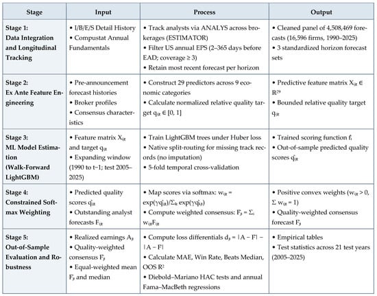
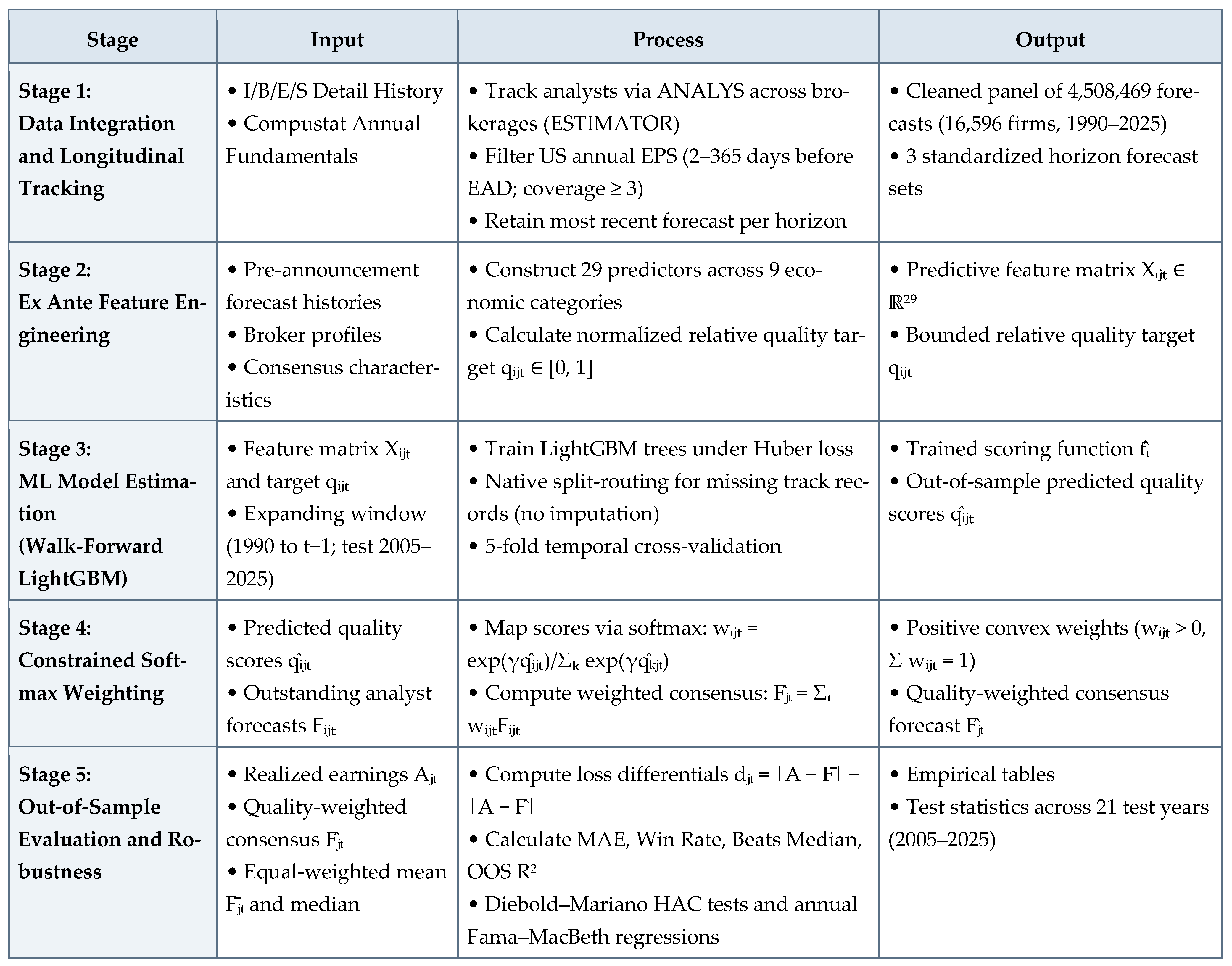

Disclaimer/Publisher’s Note: The statements, opinions and data contained in all publications are solely those of the individual author(s) and contributor(s) and not of MDPI and/or the editor(s). MDPI and/or the editor(s) disclaim responsibility for any injury to people or property resulting from any ideas, methods, instructions or products referred to in the content. |
© 2026 by the authors. Licensee MDPI, Basel, Switzerland. This article is an open access article distributed under the terms and conditions of the Creative Commons Attribution (CC BY) license.