Can Zero-Shot Large Language Models Be Trusted for Credit-Risk Prediction? An Explainability Audit Against LightGBM on Loan Default Data

Abstract

Zero-shot large language models (LLMs) offer a low-barrier route to credit-risk prediction, but regulated use requires evidence on discrimination, probability reliability, and auditable decision patterns. We compare four open-source LLMs (Gemma-2-9B, Llama-3.2-3B, Mistral-7B-v0.3, and Qwen2.5-7B) with LightGBM on 396,030 U.S. LendingClub loans issued from 2007 to 2016. Treating loans as independent and identically distributed observations from this pooled cross-sectional population, we evaluate every model on the same random 20% holdout. All models receive the same 21 structured predictors and output repayment probabilities. We audit empirical decision patterns with SHapley Additive exPlanations (SHAP); separately, each LLM supplies one context-free positive, negative, or neutral direction per feature, which we treat as its feature-level self-explanation. LightGBM achieved ROC-AUC 0.724, PR-AUC 0.907, and Brier score 0.141, compared with 0.669, 0.880, and 0.204 for the best-discriminating LLM, Gemma-2-9B. An equal-weight LightGBM–Gemma ensemble did not improve any metric. In an eight-cycle SHAP audit, each LLM shared six or seven of LightGBM’s ten most important features; these self-explanations agreed with empirical SHAP directions for only 33–67% of assessable top features, revealing self-explanation unfaithfulness under this directional criterion. A nested four-cycle estimate reproduced every LLM’s top-10 set and nearly identical importance ranks, although small magnitude and distribution shifts were statistically detectable. These results caution against standalone zero-shot LLM use in credit risk and support calibration checks, explainability audits, interpretable benchmarks, and human oversight before deployment.

1. Introduction

Credit-risk assessment sits at the core of bank lending, consumer finance, and the stability of the financial system. The quality of default prediction models directly shapes credit access, loan pricing, provisioning, and regulatory capital, and errors propagate into borrower welfare and institutional soundness. Over the past decade, machine learning (ML) methods, most prominently gradient boosting decision trees such as XGBoost (T. Chen & Guestrin, 2016) and LightGBM (Ke et al., 2017), have become the de facto standard for tabular credit scoring, combining strong discriminatory power with mature tooling for validation and interpretation.

A new class of models is now entering this space. Large language models (LLMs) such as GPT-4 have demonstrated strong performance across classification and reasoning tasks (Achiam et al., 2023; Brown et al., 2020; Vaswani et al., 2017). In a zero-shot setup, a loan application can be described in a prompt, and the model can return a repayment probability without task-specific fitting. This can reduce the task-specific training and tuning burden, but it does not eliminate data preprocessing, inference infrastructure, or independent validation. The resulting lower entry barrier may be attractive to organizations with limited modeling capacity. It also raises a question that is central to responsible adoption of artificial intelligence (AI) in finance: what empirical input–output patterns do LLM-based classifiers exhibit, and how similar are those patterns to those of validated classical models?

The question is not academic. Financial institutions operate under governance frameworks such as Basel III (Basel Committee on Banking Supervision, 2017) and the General Data Protection Regulation (European Union, 2016), under supervisory model risk management (MRM) guidance such as SR 11-7 (Board of Governors of the Federal Reserve System, 2011), and, in the European Union, under the AI Act, which classifies creditworthiness assessment as a high-risk AI application subject to transparency and human oversight obligations (European Parliament and Council, 2024). In this environment, a model whose decision logic cannot be audited, or whose separately stated feature-direction judgments are inconsistent with its measured input–output behavior, poses regulatory, reputational, and fairness risks regardless of its headline accuracy (Doshi-Velez & Kim, 2017). Unlike decision trees or gradient boosting models, LLMs are opaque systems with billions of parameters, and a growing literature questions whether model-generated explanations faithfully describe their internal computation (Huang et al., 2023; Sarkar, 2024; Turpin et al., 2023). The present study tests the behavioral faithfulness of feature-level self-explanations: whether an LLM’s separately elicited global feature direction agrees with its empirical SHAP direction. This operational test does not reveal the model’s internal computation.

This paper addresses these concerns through a systematic, audit-oriented comparison of zero-shot LLM classifiers and LightGBM on a real-world LendingClub loan default task. Both model families receive identical structured inputs and are evaluated on the same random-holdout observations, for which they output repayment probabilities. We then treat explainability as a model validation exercise: SHapley Additive exPlanations (SHAP) (Lundberg & Lee, 2017) provide a model-agnostic empirical account of which features drive each model’s predictions. In a separate feature-level elicitation, each LLM supplies one context-free positive, negative, or neutral direction for each predictor. We treat each one-off, context-free direction response as a feature-level self-explanation and audit its faithfulness against the corresponding SHAP dependence pattern. Here, self-explanation unfaithfulness means disagreement between the model’s stated feature direction and its empirical SHAP direction under the prespecified rule. We do not collect per-loan explanations or free-text rationales, and do not infer the model’s internal reasoning from this behavioral test. Concretely, we ask:

• RQ1 (Performance). How do zero-shot LLMs compare with a LightGBM benchmark in discrimination (ROC-AUC and PR-AUC) and probability reliability (Brier score and reliability diagrams), and does ensembling the two paradigms improve performance?
• RQ2 (Explainability). Do LLM-based classifiers prioritize the same credit-risk drivers as the classical benchmark, in both magnitude and direction?
• RQ3 (Self-explanation faithfulness). Are the LLMs’ one-off, context-free feature-direction self-explanations faithful to their empirical SHAP directions?

Our contributions are threefold. First, we provide, to our knowledge, the first head-to-head comparison of zero-shot LLMs and LightGBM on structured loan data in which SHAP attributions are computed for the LLMs themselves and used to audit the faithfulness of separately elicited, context-free feature-direction self-explanations. Second, we document systematic divergences between LLM and classical decision patterns, including reversed directional effects for economically meaningful variables such as the interest rate and the debt-to-income (DTI) ratio, and cases in which an LLM’s single general direction does not describe its full SHAP dependence pattern. Third, we translate these findings into concrete implications for credit-risk governance, arguing that zero-shot LLMs should currently be treated as unvalidated challenger models whose deployment requires independent explainability audits, interpretable benchmarks, and human-in-the-loop oversight.

The remainder of the paper is organized as follows. Section 2 reviews the literature on LLM classification, LLM explainability, tabular learning, and explainable AI (XAI) in credit risk, and positions our work within model risk management practice. Section 3 describes the data, models, and the SHAP-based audit methodology. Section 4 presents the empirical results. Section 5 discusses implications for credit-risk management and regulation, together with limitations and future research. Section 6 concludes.

2. Literature Review

2.1. LLMs for Zero-Shot Classification and Regression

LLMs have demonstrated strong classification capabilities, often achieving competitive performance without supervision. Brown et al. (2020) introduced GPT-3, highlighting its few-shot and zero-shot classification potential. Zero-shot prompting avoids task-specific parameter fitting, although practical use still requires data preparation, inference infrastructure, output validation, and domain oversight. Subsequent work has explored structured prompting to enhance classification accuracy: Wei et al. (2022) introduced chain-of-thought prompting, showing that eliciting structured reasoning improves LLM performance, which is relevant when adapting these models to structured data. A recent line of work examines whether LLMs can function as regressors for numerical data. Vacareanu et al. (2024) found that LLMs approximate regression functions with in-context examples, while Buckmann and Hill (2024) proposed combining LLMs with logistic regression for low-data robustness. Song et al. (2024) and Song and Bahri (2025) further extend this research direction, demonstrating universal regression capabilities using decoding-based inference. Our loan repayment task builds on this literature by asking the LLM to act as a probability regressor over structured borrower attributes, but unlike prior studies that evaluate LLM classification in isolation, we position the comparison as a step toward responsible AI deployment in a regulated, high-stakes financial domain.

2.2. LLM-Generated Explanations and Feature-Direction Elicitation

Feature-attribution methods such as SHAP (Lundberg & Lee, 2017) are widely used to assess feature importance in machine learning models. A key open question is whether claims elicited from LLMs about their behavior align with the features that actually drive their outputs. Huang et al. (2023) report that LLM rationales are often plausible but do not necessarily reflect internal reasoning. Dehghanighobadi et al. (2025) analyze counterfactual explanations and show that LLMs can struggle with causal dependencies. Sarkar (2024) argues that LLMs lack self-explanatory capabilities due to opaque training dynamics, and Turpin et al. (2023) show that chain-of-thought explanations can be systematically misleading. Prior work predominantly studies generated textual explanations in language tasks. Our prediction prompt, by contrast, requests only a probability and does not request an explanation. The additional evidence examined here is also narrower than a textual rationale: in a separate prompt, each model supplies one general direction label for each feature. To our knowledge, our study is the first to compute SHAP-based feature importance for LLMs prompted to output probabilistic predictions on structured financial data and to compare those attributions with separately elicited global feature directions. We regard the one-off direction response itself as a feature-level self-explanation, even though it contains no free-text rationale. Directional disagreement with the model’s empirical SHAP behavior constitutes self-explanation unfaithfulness under our operational criterion; it does not reveal the model’s internal reasoning.

2.3. LLMs for Tabular Data

Recent work explores whether LLMs can replace gradient-boosted models for tabular classification. Fang et al. (2024) survey LLMs on tabular data and highlight adaptation challenges. Ghaffarzadeh-Esfahani et al. (2024) benchmark LLMs against classical ML for COVID-19 mortality prediction, concluding that classical models outperform LLMs on structured data, and C. Chen et al. (2024) reach a similar conclusion for clinical prediction with ClinicalBench. Hegselmann et al. (2023) propose TabLLM, which reformulates tables as natural language for few-shot classification, while Shi et al. (2024) treat autoregressive LLMs as feature-embedding models for tabular prediction. While these studies highlight LLM potential, they generally do not compare empirical feature attributions with separately elicited feature-direction judgments on tabular tasks, which is the narrower focus of the present paper.

2.4. Explainable AI in Credit Risk

Explainability is a long-standing requirement in financial risk applications. Martins et al. (2023) review XAI in finance, while Černevičienė and Kabašinskas (2024), Misheva et al. (2021), and Bussmann et al. (2021) analyze explainability in credit-risk modeling specifically. Several studies benchmark ML models for loan default prediction: Madaan et al. (2021) compare decision trees and random forests without an explainability analysis; Srinivasa Rao et al. (2021) assess ML techniques for loan risk but do not explore LLMs; and Boughaci and Alkhawaldeh (2020) study credit scoring models without evaluating LLM-based predictions. We extend this literature with the first comparative analysis of LLMs and LightGBM on structured loan data that integrates SHAP-based explainability for both model families.

2.5. Model Risk Management and the Responsible AI Gap

Most tabular-LLM studies prioritize accuracy and prompting strategies but rarely audit whether separately elicited claims about general feature direction agree with the model’s empirical prediction patterns or are suitable for model validation in credit settings. In particular, they rarely (i) compare elicited feature directions with model-agnostic attributions such as SHAP, (ii) situate results within model risk management practice, or (iii) examine compliance implications, despite credit scoring being a regulated activity that the EU AI Act classifies as high-risk AI with duties of transparency and human oversight (European Parliament and Council, 2024), and despite supervisory expectations on loan origination model governance (European Banking Authority, 2020).

Our audit protocol is designed to mirror banking MRM practice, which requires robust model development, independent validation, and ongoing monitoring (Board of Governors of the Federal Reserve System, 2011; Office of the Comptroller of the Currency, 2021), and is consistent with horizontal AI risk guidance (International Organization for Standardization, 2023; National Institute of Standards and Technology, 2023) and with public-private supervisory work on AI in financial services (Bank of England and Financial Conduct Authority, 2022). In this protocol, SHAP is not treated as causal ground truth but as a consistent, model-agnostic operational reference for comparing a model’s elicited general feature directions with its empirical prediction patterns, in the spirit of transparency artifacts such as model cards and datasheets (Gebru et al., 2021; Mitchell et al., 2019). We use this comparison to audit self-explanation faithfulness: a context-free feature-direction response is unfaithful when it disagrees with the model’s empirical SHAP direction under the stated rule. This behavioral criterion does not establish causality or reveal internal reasoning.

3. Data and Methodology

3.1. Comparative Audit Framework

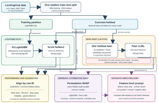
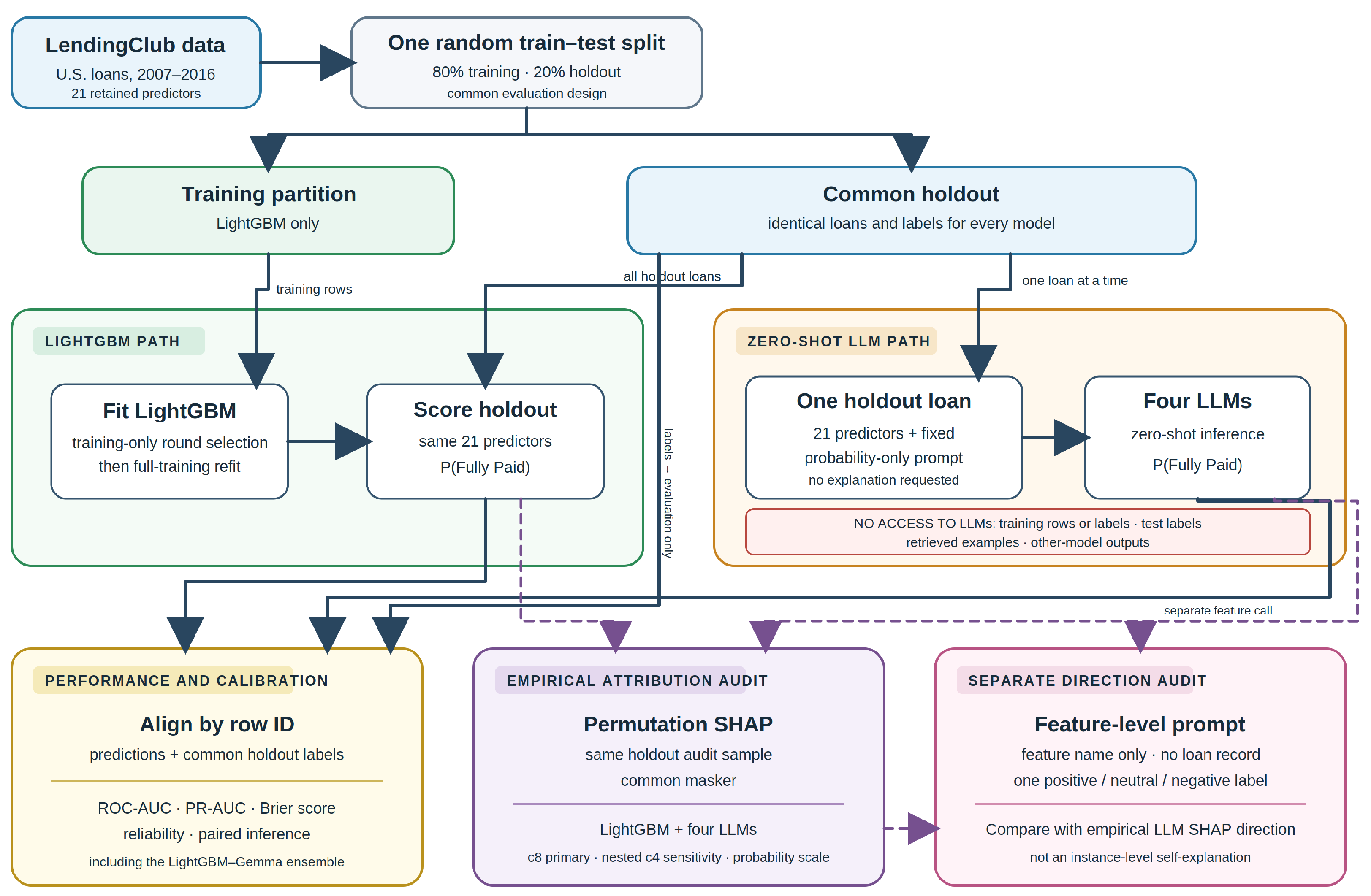
Figure 1 illustrates the overall framework. A single random train–test partition is created before the two model pipelines diverge. The 80% training partition is used to fit LightGBM only. The remaining 20% is a common evaluation set: LightGBM produces predictions for these observations, while each zero-shot LLM receives each of these same observations as a separate natural-language prompt. The LLMs are never given the LightGBM training records, training labels, test labels, or LightGBM outputs. Predictions from every model are aligned to the same test labels by row identifier. Thus, both LightGBM and the LLMs receive the same 21 predictors for every evaluated loan and output probability estimates of full repayment instead of discrete classes. Probability outputs offer three advantages: (i) fine-grained evaluation via discrimination metrics (ROC-AUC, PR-AUC); (ii) enhanced explainability, as SHAP feature attribution is generally more informative when applied to probability scores rather than hard labels; and (iii) a direct test of LLMs’ capability as probability regressors. Both pipelines are then analyzed for predictive performance and empirical feature attribution through SHAP. A separate feature-level prompt supplies the LLM directional judgments used in the descriptive alignment audit; it is not part of the per-loan prediction prompt.

Figure 1. Comparative explainable AI framework: LightGBM vs. zero-shot LLMs. One random 80%/20% partition is made before the model paths diverge. The training partition is used only for LightGBM model selection and fitting. The fitted LightGBM and all four LLMs score the same holdout loans; each LLM receives one loan at a time through the fixed probability-only prompt and has no access to training rows or labels, test labels, retrieved examples, or other-model outputs. Predictions are aligned with the common-holdout labels for performance, calibration, paired inference, and the LightGBM–Gemma ensemble. Both model families undergo the empirical permutation-SHAP audit; separately, each LLM supplies one context-free direction per feature through a feature-level prompt with no loan record or rationale.

3.2. Data

3.2.1. Task Description

Loan default prediction is a critical challenge in credit-risk assessment, where lenders estimate the likelihood of borrowers failing to repay their loans. Accurate predictions enable financial institutions to make informed lending decisions, set appropriate interest rates, and manage credit risk effectively. Because loan defaults directly affect credit access, financial stability, and regulatory compliance, this task is widely regarded as a high-stakes benchmark for testing the safety and reliability of predictive models in finance.

3.2.2. Dataset

We use publicly available U.S. LendingClub loan records obtained from Kaggle.1 The dataset contains 396,030 loan records issued between 2007 and 2016. Each loan is labeled with its repayment status, distinguishing between Fully Paid and Charged Off (defaulted) loans. It contains both numerical and categorical attributes describing borrower creditworthiness and loan characteristics, for a total of 26 financial and credit-related features.

3.2.3. Preprocessing

We removed five features due to high cardinality, redundancy, or potential data leakage:

• issue_d: Loan issue date (excluded from the predictor set because calendar time is outside the pooled cross-sectional estimand and is provided to neither model)
• earliest_cr_line: Borrower’s earliest credit line (high cardinality)
• address: High-cardinality feature (introduces geographic bias)
• emp_title: High-cardinality categorical variable
• title: High-cardinality; redundant with the purpose variable

We also excluded categorical features with more than 40 unique categories to reduce sparse high-cardinality inputs. Applying the same retained feature set to every model prevents direct use of calendar-time and address-derived signals and keeps the comparison focused on the same 21 structured predictors. This input standardization supports a controlled comparison; it should not be interpreted as a fairness assessment.

3.2.4. Final Dataset and Common Holdout

After preprocessing, 21 predictors remain (12 numerical and 9 categorical). We randomly selected a 20% (79,206 samples) holdout test set, with the remaining 80% used for training. LightGBM selection and fitting use only the training partition, whereas every model is evaluated on the same holdout. LLM prompts are generated exclusively from the holdout predictors, and predictions are aligned to the common labels before evaluation or ensembling. Thus, comparisons are paired observation by observation, test labels play no role in LightGBM model selection, and no LLM has access to the LightGBM training partition during prediction.

Why a Random Rather than Temporal Split?

The observational unit in this study is an individual loan, not a point in a modeled time series. We do not use loan histories as temporal sequences, lagged outcomes, rolling windows, or autoregressive predictors. Our estimand is the relative in-distribution performance and decision logic of LightGBM and zero-shot LLMs for the pooled 2007–2016 study population. For this estimand, we assume that loan records are independent draws from a common pooled distribution and therefore treat them as exchangeable. A random holdout is appropriate under this assumption because it preserves a common input distribution while isolating model-family differences on the same observations. A chronological split would instead estimate transport to a later origination cohort under possible economic and policy drift, which is an important but distinct forecasting and deployment question. We accordingly make no claim that the random-holdout results establish out-of-time robustness; prospective deployment would require a separate temporal validation under the intended operating conditions.

Table 1 lists all features. For numerical features, we report the interval bounded by the 1st and 99th percentiles. For categorical features, we report the value space (if it is not too large).

Table 1. Final dataset features.

Feature Description	Range
Loan amount	[1600.0, 35,000.0]
Term	categorical: {36 months, 60 months}
Interest rate	[6.03, 25.29]
Installment	[55.32, 1204.57]
Grade	categorical: {A, B, C, D, E, F, G}
Sub-grade	categorical: {A1, A2, …, G4, G5}
Employment length	categorical: {<1 year, 1 year, …, 10+ years}
Home ownership	categorical: {MORTGAGE, NONE, OTHER, OWN, RENT}
Annual income	[19,000.0, 250,000.0]
Verification status	categorical: {Not Verified, Source Verified, Verified}
Purpose	categorical: 14 values (e.g., wedding)
Debt-to-income (DTI) ratio	[1.6, 36.41]
Open credit accounts	[3.0, 27.0]
Public records	[0.0, 2.0]
Revolving balance	[169.05, 83,505.9]
Revolving utilization rate	[1.2, 98.0]
Total accounts	[6.0, 60.0]
Initial listing status	categorical: {f, w}
Application type	categorical: {DIRECT PAY, INDIVIDUAL, JOINT}
Mortgage accounts	[0.0, 9.0]
Public record bankruptcies	[0.0, 1.0]

3.3. Models

3.3.1. LightGBM Benchmark

We trained a LightGBM classifier using the gradient boosting decision tree (GBDT) algorithm with a binary objective and AUC as the model-selection metric. The training partition was split internally (80/20, stratified) for early stopping round selection, after which the selected 1650 boosting rounds were refit on the full training partition. The model uses a learning rate of 0.01, feature and bagging fractions of 0.8, L1/L2 regularization of 0.1 each, 63 leaves, and a minimum of 50 observations per leaf. The common holdout is not used for early stopping or model selection. We use LightGBM as an interpretable benchmark against which the behavior of the LLMs can be audited.

3.3.2. LLM Inference

We evaluated four recent open-source instruction-tuned LLMs: Gemma-2-9B-Instruct (Gemma Team et al., 2024), Llama-3.2-3B-Instruct (Meta AI, 2024), Mistral-7B-Instruct-v0.3 (Jiang et al., 2023), and Qwen2.5-7B-Instruct (Yang et al., 2024). Model weights were obtained from the Hugging Face Hub (Wolf et al., 2020).

Inference was run on a Kubernetes cluster using NVIDIA Dynamo and the vLLM inference engine, with 32 NVIDIA H100 GPUs, each equipped with 80 GiB of GPU memory.

We did not perform any fine-tuning or in-context learning. At inference time, an LLM receives only the 21 feature values for one holdout observation and the fixed task instructions; it receives no training records, labels, retrieved examples, or predictions from another model. We use the same prompt template for all LLMs. The per-loan prediction prompt asks only for a repayment probability and does not request an explanation or rationale. The separate feature-level direction prompt is not conditioned on an individual loan; it asks each model for one general positive, negative, or neutral direction for each feature.

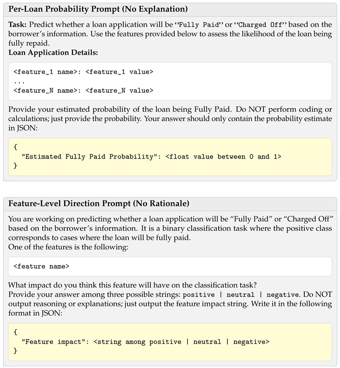
Neither prompt schema requests a free-text rationale. The feature-level direction response itself is the self-explanation evaluated in our faithfulness audit; the per-loan probability response contains no explanation.

3.4. Predictive Evaluation and Statistical Inference

We define Fully Paid as the positive class and evaluate raw, uncalibrated probabilities on the common holdout. Outputs are required to contain a valid probability in $[0,1]$; no record is dropped or imputed. The prespecified ensemble is the unweighted arithmetic mean of the aligned LightGBM and Gemma-2-9B probabilities.

We report ROC-AUC and average precision (hereafter PR-AUC) as discrimination measures. Probability accuracy is measured by the binary Brier score (BS),

$$BS={\displaystyle \frac{1}{n}}{\displaystyle \sum _{i=1}^n}{(p_i-y_i)}^2,$$

(1)

where n is the number of samples, $p_i$ is the predicted probability of full repayment and $y_i\in \{0,1\}$ is the observed outcome. It is the mean squared probability error and a strictly proper scoring rule: its expected value is minimized by reporting the true event probability. It ranges from 0 (perfect) to 1 for binary outcomes, and lower values are better. The prevalence of Fully Paid in the common test set is 0.8033. This is the expected PR-AUC of a non-informative random ranking; a separate constant forecast equal to that prevalence has Brier score $0.8033(1-0.8033)=0.1580$ and provides a probability-error reference. Calibration is evaluated without post-hoc Platt or isotonic fitting. Reliability diagrams use 10 fixed equal-width probability bins on $[0,1]$, plotting the mean prediction against the observed positive rate; agreement with the diagonal indicates calibration at the displayed bin resolution. Vertical error bars are 95% Wilson intervals for the observed rate, and gray bars show bin support. As a descriptive summary, we report the Expected Calibration Error (ECE),

$$ECE={\displaystyle \sum _{k=1}^K}{\displaystyle \frac{n_k}{n}}\left|{\overline{p}}_k-{\overline{y}}_k\right|,$$

(2)

where K is the number of bins, $n_k$ is the number of loans in bin k, ${\overline{p}}_k$ is their mean predicted probability, and ${\overline{y}}_k$ is their observed positive rate. It is the bin-support-weighted absolute gap between mean prediction and observed rate. Lower values indicate closer bin-level agreement, but ECE depends on the chosen binning rule.

Uncertainty and model comparisons use 2000 paired, stratified nonparametric bootstrap resamples of loans. Positive and negative observations are resampled separately to preserve the test-set class balance. The resampling unit is the complete aligned loan record—its outcome and every model’s prediction—so the identical loans enter each model comparison in every replicate. This pairing preserves the within-loan dependence between model results and estimates the sampling distribution of their difference directly. We use 95% percentile confidence intervals for ROC-AUC, PR-AUC, Brier score, and model-minus-LightGBM differences. Two-sided comparison p-values are twice the smaller empirical sign-tail probability, with a $+1$ finite-resample correction; Holm’s method controls multiplicity across the five comparisons within each metric. A positive difference favors the comparator for ROC-AUC and PR-AUC, whereas a negative difference favors it for Brier score. These intervals describe finite-holdout uncertainty conditional on the fitted models and observed class balance; they do not include retraining, prompt/model-version variation, or temporal transport uncertainty.

3.5. Explainability as a Model Audit

We treat explainability as a model-auditing task focused on the faithfulness of feature-level self-explanations to empirical input–output behavior. Our audit has two complementary components:

• (A) SHAP as a model-agnostic audit baseline. We use SHAP (Lundberg & Lee, 2017) to assign contribution values to each feature for both LightGBM and the LLM-based probabilistic classifier. SHAP values operationalize which features, and in what direction, are driving each model’s predictions.
• (B) Feature-level self-explanations via directional elicitation. Independently of the loan-level prediction calls, we ask each LLM once about each of the 21 input features and record one general positive, negative, or neutral direction. The resulting 21 labels per model (84 in total) are the self-explanations being audited; they contain no textual justification and are not tied to individual test observations.

We compare (i) global feature importance patterns via SHAP across models; (ii) directional dependence for key features (e.g., whether higher values increase or decrease repayment probability); and (iii) each elicited global direction with the corresponding model’s SHAP dependence pattern. We operationalize self-explanation faithfulness as agreement between the elicited direction and the empirical SHAP direction, and classify disagreement as self-explanation unfaithfulness. A single global label cannot represent nonlinear or value-dependent effects fully, which limits the scope of this criterion. The audit does not test instance-level coherence, evaluate free-text rationales, or reveal the model’s internal computation.

3.5.1. Permutation-SHAP Design and Convergence Audit

We estimate post hoc attributions using SHAP’s model-agnostic permutation explainer (Lundberg & Lee, 2017). The response is the predicted probability of Fully Paid, so every base value and SHAP contribution is expressed on the probability scale. We draw a fixed subsample of 1000 loans from the common holdout. All models use the same observations, feature order, encoding, and masker, which is constructed from five k-means centroids.

The primary estimate uses eight forward–reverse permutation cycles per loan. A nested four-cycle estimate uses the same observations, masker, and randomization, allowing a paired sensitivity comparison. Invalid probability responses are not imputed.

The convergence audit reports (i) Spearman correlation between the 21 global mean-absolute-SHAP importance vectors, (ii) top-10 overlap, (iii) a paired Wilcoxon test of each loan’s mean-absolute-SHAP magnitude, and (iv) the maximum absolute gap between the aggregate four- and eight-cycle empirical distributions, assessed with a paired loan-level randomization test. Holm adjustment is applied across the four LLMs separately within the magnitude and distribution test families. We report statistically detectable differences even when their practical size is small and rank-based conclusions are unchanged.

Global importance is the mean absolute eight-cycle SHAP value over the audit sample. The feature-direction audit uses the ten features ranked highest by LightGBM under this definition. For an ordered or numerical feature, the empirical SHAP direction for each model is considered positive when the Spearman correlation between its feature values and SHAP contributions exceeds 0.10, negative when it is below $-0.10$, and neutral/weak otherwise. We do not impose an artificial order on unordered categorical features; such entries are reported as not assessed. This rule compares two global summaries and does not turn the elicited label into an instance-level explanation.

3.5.2. Feature-Level Directional Elicitation

For each LLM, we issue the feature-level prompt once for each of the 21 input features. The prompt identifies one feature and asks whether it will generally affect the predicted likelihood of full repayment positively, negatively, or neutrally. The only recorded field is Feature impact; no loan values, loan identifier, probability prediction, free-text explanation, or textual justification is included. Each response is therefore a model-level, context-free self-explanation of one feature’s direction of influence, elicited once per feature rather than for an individual loan.

We compare each elicited direction with the broad direction of the same model’s SHAP dependence pattern. SHAP is used as an operational, model-agnostic description of prediction behavior, not as causal ground truth. Likewise, an elicited direction is not evidence about the model’s internal reasoning. A mismatch between the elicited direction and the empirical SHAP direction, defined by the prespecified Spearman rule, is evidence of self-explanation unfaithfulness in this feature-level behavioral sense. Nonlinearity and the limits of a context-free sign may help explain such mismatches, but do not make the stated direction faithful under this criterion. The claim concerns the elicited direction response itself, not an uncollected free-text rationale or an internal reasoning trace.

4. Empirical Results

4.1. Predictive Performance

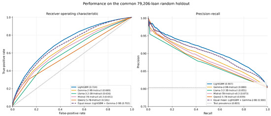
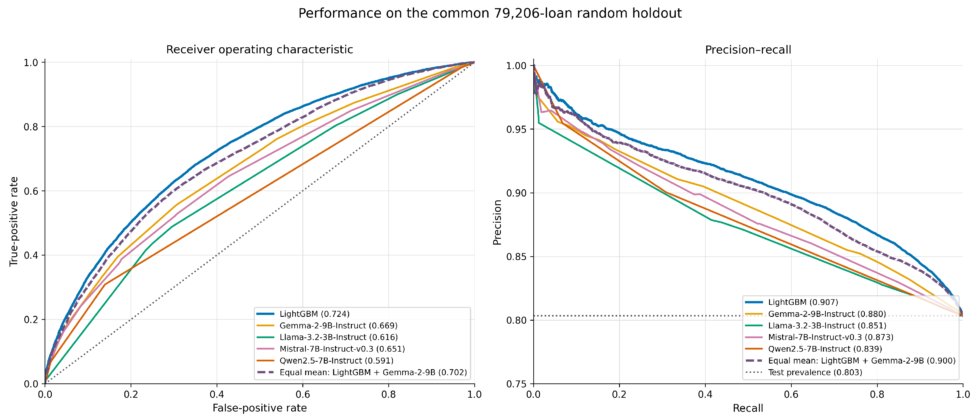
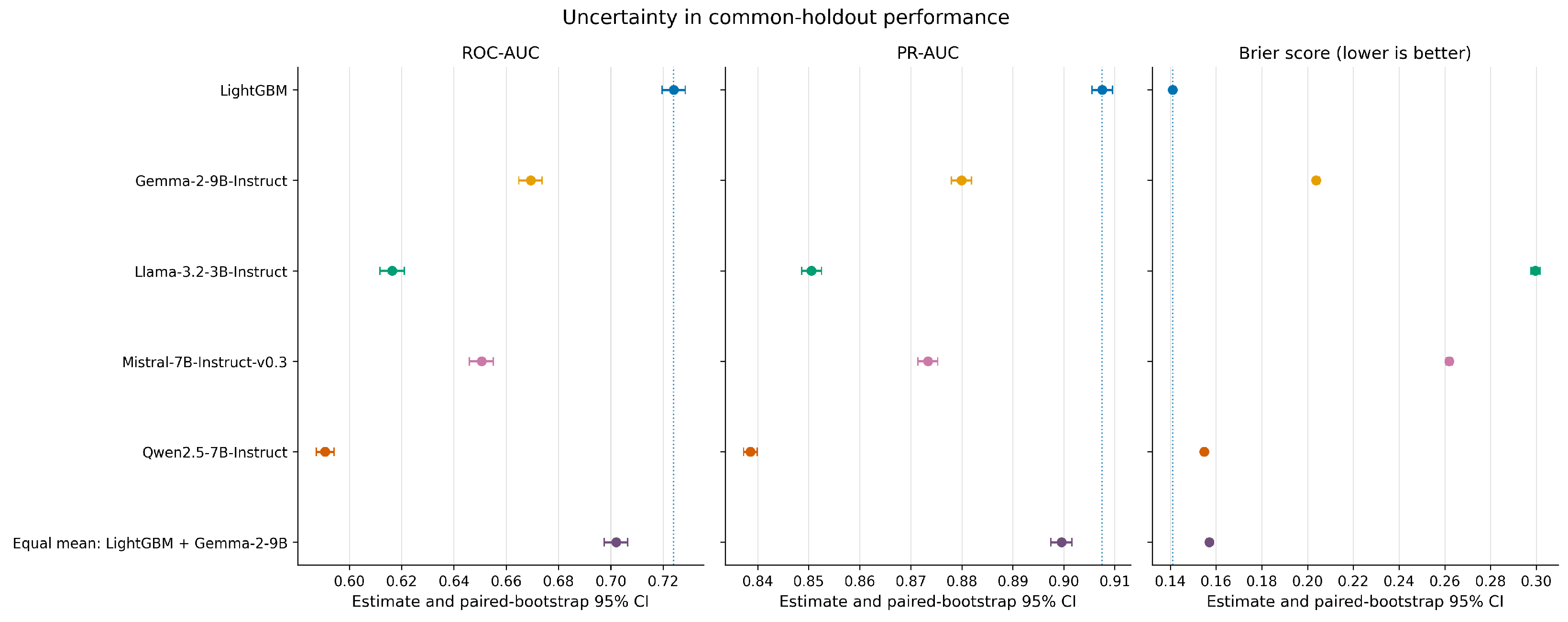
Table 2 and Figure 2 compare all models on the common holdout. LightGBM achieved the highest ROC-AUC, 0.7240 (95% CI [0.7197, 0.7284]), and PR-AUC, 0.9075 [0.9055, 0.9096]. Gemma-2-9B was the strongest LLM on both discrimination measures, with ROC-AUC 0.6693 [0.6648, 0.6738] and PR-AUC 0.8799 [0.8779, 0.8819]. It was followed by Mistral-7B-v0.3, Llama-3.2-3B, and Qwen2.5-7B. These results are consistent with prior evidence that gradient boosting often surpasses deep learning methods on structured tabular data (C. Chen et al., 2024; Ghaffarzadeh-Esfahani et al., 2024).

Table 2. Common-holdout performance. Entries are point estimates with paired stratified-bootstrap 95% confidence intervals in brackets. Fully Paid is positive; its test prevalence is 0.8033. A lower Brier score is better. Bold indicates the best result.

Model	ROC-AUC [95% CI]	PR-AUC [95% CI]	Brier [95% CI]
LightGBM	0.7240 [0.7197, 0.7284]	0.9075 [0.9055, 0.9096]	0.1410 [0.1403, 0.1418]
Gemma-2-9B-Instruct	0.6693 [0.6648, 0.6738]	0.8799 [0.8779, 0.8819]	0.2038 [0.2025, 0.2052]
Llama-3.2-3B-Instruct	0.6163 [0.6117, 0.6210]	0.8505 [0.8486, 0.8525]	0.2996 [0.2976, 0.3016]
Mistral-7B-Instruct-v0.3	0.6506 [0.6459, 0.6552]	0.8734 [0.8714, 0.8753]	0.2619 [0.2607, 0.2631]
Qwen2.5-7B-Instruct	0.5907 [0.5873, 0.5943]	0.8385 [0.8372, 0.8399]	0.1548 [0.1545, 0.1551]
Equal mean: LightGBM + Gemma-2-9B	0.7020 [0.6975, 0.7065]	0.8996 [0.8975, 0.9016]	0.1570 [0.1562, 0.1579]

Figure 2. ROC and precision–recall curves on the common random holdout. Legend values are ROC-AUC (left) and PR-AUC (right). The dotted diagonal is the no-skill ROC reference; the dotted horizontal line in the precision–recall panel is the 0.803 test prevalence of the positive class (Fully Paid). The ensemble is the equal-weight mean of aligned LightGBM and Gemma-2-9B probabilities.

The equal-weight LightGBM–Gemma ensemble reached ROC-AUC 0.7020 [0.6975, 0.7065] and PR-AUC 0.8996 [0.8975, 0.9016], below LightGBM alone. All models exceeded the test prevalence of 0.8033, the non-informative reference for PR-AUC with Fully Paid as the positive class. Prevalence is a metric reference rather than a fitted baseline model, so neither it nor a random classifier is included as a row in Table 2.

4.2. Calibration and Paired Model Comparisons

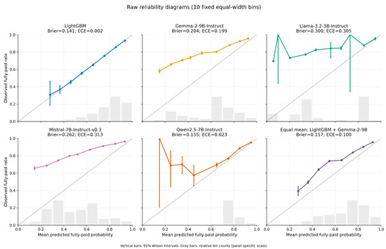
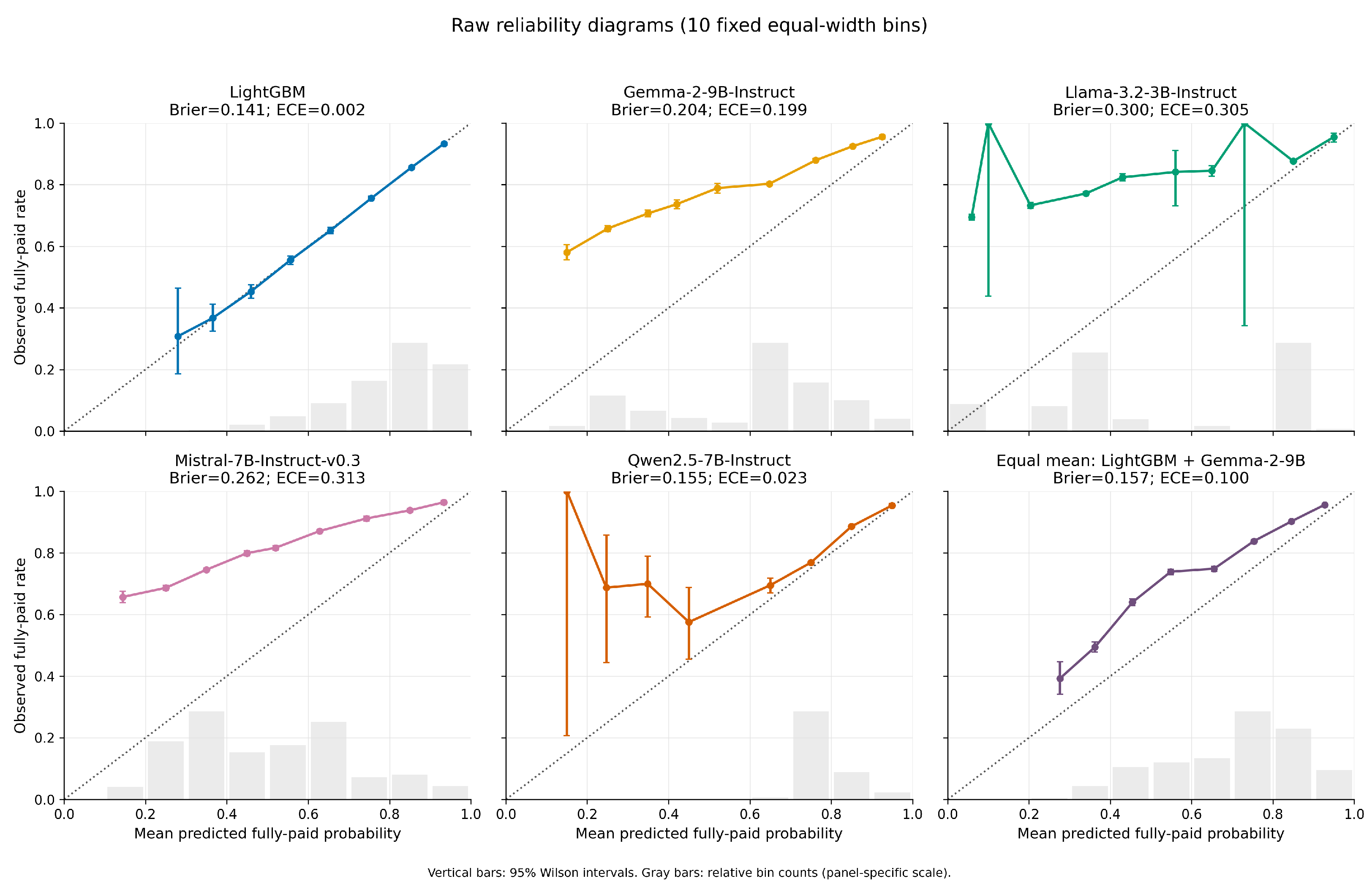
Discrimination and probability reliability lead to different conclusions about the LLMs. For context, predicting the test prevalence (0.8033) for every loan gives a Brier score of 0.1580. LightGBM had the lowest Brier score, 0.1410 [0.1403, 0.1418], and its reliability curve closely followed the identity line (ECE 0.0016). Qwen2.5-7B had the second-lowest Brier score, 0.1548 [0.1545, 0.1551], and ECE 0.0226, even though it had the weakest ROC-AUC and PR-AUC. Its near-baseline Brier result therefore should not be read as strong loan-level ranking: predictions close to a high base rate can have modest squared error while discriminating poorly. In contrast, Gemma-2-9B was the strongest-ranking LLM but had Brier score 0.2038 and ECE 0.1994, both indicating substantially less reliable raw probabilities. Llama-3.2-3B and Mistral-7B-v0.3 were substantially underconfident over densely populated probability ranges, with Brier scores of 0.2996 and 0.2619 and ECE values of 0.3045 and 0.3125, respectively. The equal-weight ensemble’s Brier score of 0.1570 was slightly below the constant-forecast reference but remained worse than LightGBM. Thus, ranking quality and numerical probability reliability are not interchangeable, and a single headline metric would obscure the models’ different failure modes.

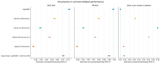
Figure 3 reports the raw reliability curves. Fixed bins with little support produce wide Wilson intervals, especially at the low-probability end for Llama and Qwen, so those isolated bin rates should not be overinterpreted. No post-hoc calibration model was fitted to the test set. Figure 4 separately displays the metric confidence intervals.

Figure 3. Reliability diagrams for raw model probabilities using 10 fixed equal-width bins. The diagonal denotes perfect calibration; points compare the mean predicted probability with the observed Fully Paid rate. Vertical bars are 95% Wilson intervals, and gray bars show relative bin counts on a panel-specific scale. Brier score and 10-bin ECE are displayed for context; lower values indicate smaller error.

Figure 4. ROC-AUC, PR-AUC, and Brier point estimates with 95% paired stratified-bootstrap confidence intervals on the common holdout. Dotted vertical lines mark the LightGBM point estimate in each panel. Higher ROC-AUC and PR-AUC are better; lower Brier score is better.

Table 3 reports paired differences against LightGBM. All intervals exclude zero in the direction favoring LightGBM, including the ensemble comparison. Each two-sided bootstrap sign-tail test remains significant after the prespecified Holm correction across five comparisons within its metric ($p_{\mathrm{Holm}}=0.005$ after rounding). The ensemble therefore offers no gain in discrimination or probability accuracy on this holdout.

Table 3. Paired model comparisons against LightGBM. Differences are comparator minus LightGBM, with 95% paired stratified-bootstrap intervals. Positive differences favor the comparator for ROC-AUC and PR-AUC; negative differences favor it for Brier score. The final column gives the Holm-adjusted two-sided p-value for each of the three metric comparisons in that row (unrounded value 0.004998).

Comparator	$\mathbf{\Delta }$ ROC-AUC [95% CI]	$\mathbf{\Delta }$ PR-AUC [95% CI]	$\mathbf{\Delta }$ Brier [95% CI]	Holm p
Gemma-2-9B-Instruct	$-0.0547$ [$-0.0579$, $-0.0515$]	$-0.0275$ [$-0.0289$, $-0.0262$]	$+0.0627$ [$+0.0617$, $+0.0638$]	0.005
Llama-3.2-3B-Instruct	$-0.1077$ [$-0.1121$, $-0.1032$]	$-0.0569$ [$-0.0589$, $-0.0549$]	$+0.1585$ [$+0.1567$, $+0.1604$]	0.005
Mistral-7B-Instruct-v0.3	$-0.0734$ [$-0.0772$, $-0.0695$]	$-0.0341$ [$-0.0357$, $-0.0325$]	$+0.1209$ [$+0.1198$, $+0.1220$]	0.005
Qwen2.5-7B-Instruct	$-0.1333$ [$-0.1375$, $-0.1293$]	$-0.0690$ [$-0.0707$, $-0.0674$]	$+0.0138$ [$+0.0131$, $+0.0145$]	0.005
Equal mean: LightGBM + Gemma-2-9B	$-0.0220$ [$-0.0241$, $-0.0201$]	$-0.0079$ [$-0.0088$, $-0.0070$]	$+0.0160$ [$+0.0155$, $+0.0165$]	0.005

4.3. SHAP Feature Importance and Permutation-Budget Sensitivity

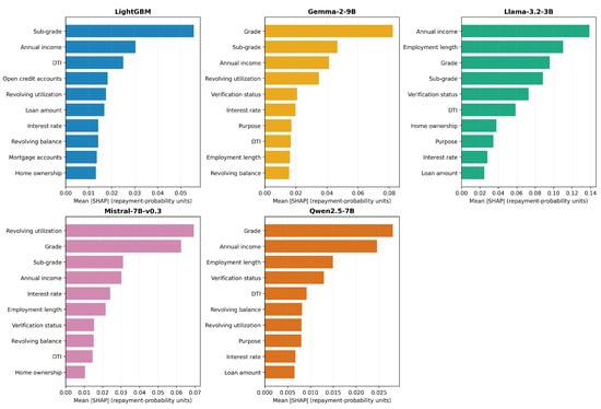
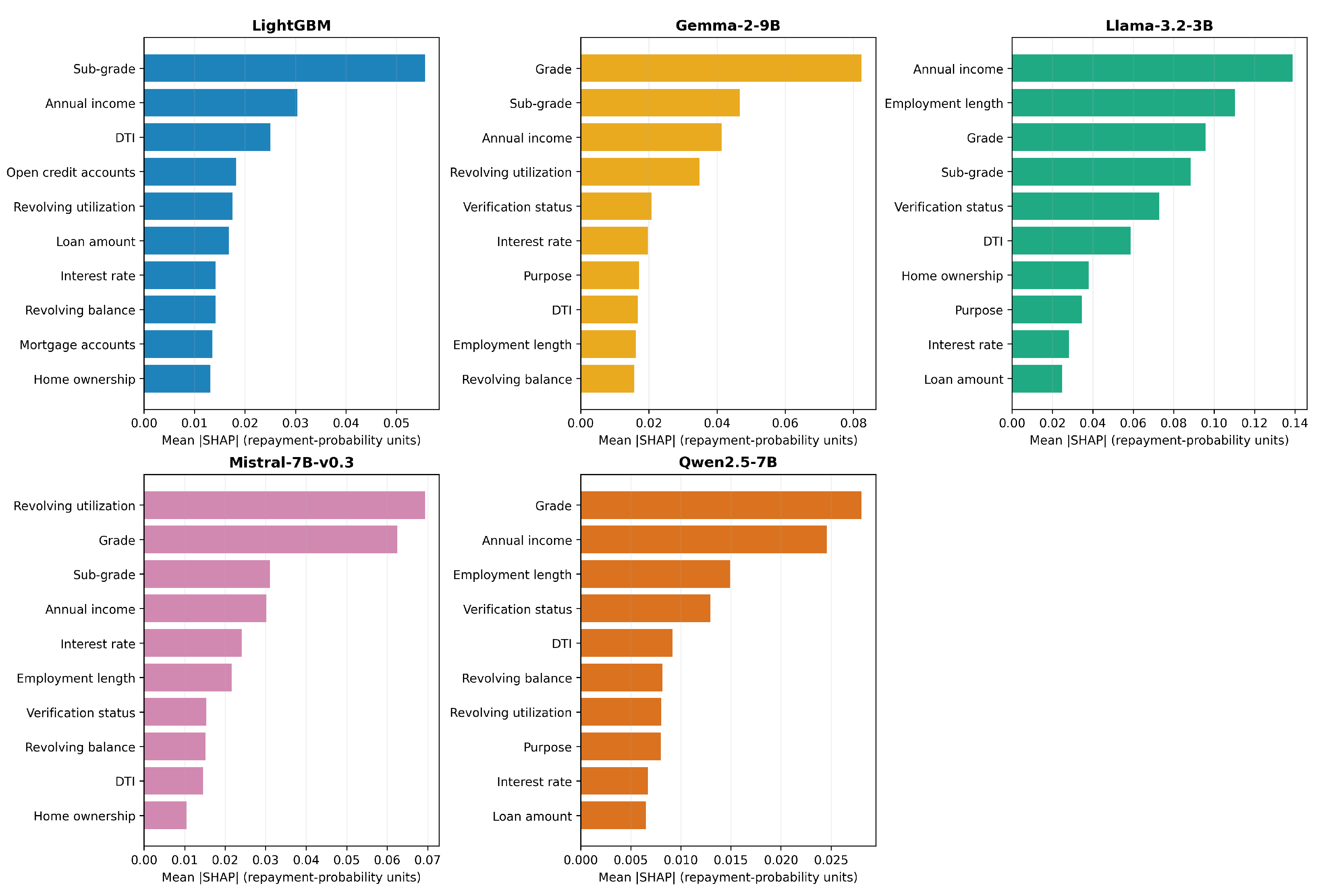
The eight-cycle estimates reveal partial, rather than near-complete, agreement between the benchmark and LLM importance profiles. Each LLM shares six or seven of LightGBM’s ten highest-ranked features. Across all 21 features, the LightGBM–LLM Spearman rank correlations range from 0.444 to 0.571. The LLMs are more similar to one another (pairwise correlations 0.807–0.956 and eight or nine shared top-10 features), but they still assign substantially different magnitudes and ranks. LightGBM’s three largest global attributions are Sub-grade, Annual income, and DTI; the leading LLM feature is Grade for Gemma-2-9B and Qwen2.5-7B, Annual income for Llama-3.2-3B, and Revolving utilization for Mistral-7B-v0.3. Figure 5 shows each model’s own top ten, while Table 4 compares all models on the ten features selected by the LightGBM ranking.

Figure 5. Eight-cycle global SHAP importance on the common audit sample. Each panel shows the model’s ten largest mean-absolute-SHAP values; values are changes in predicted Fully Paid probability under the common masker. Panel-specific horizontal scales preserve within-model rankings, so bar lengths should not be compared visually across panels without consulting the numeric table.

Table 4. Eight-cycle mean-absolute-SHAP values for LightGBM’s ten highest-ranked features, in predicted-repayment-probability units. Rows follow the LightGBM ranking.

Feature	LightGBM	Gemma-2-9B	Llama-3.2-3B	Mistral-7B-v0.3	Qwen2.5-7B
Sub-grade	0.0557	0.0467	0.0884	0.0311	0.0054
Annual income	0.0303	0.0414	0.1390	0.0302	0.0246
DTI	0.0250	0.0168	0.0587	0.0145	0.0092
Open credit accounts	0.0182	0.0044	0.0082	0.0073	0.0029
Revolving utilization	0.0175	0.0349	0.0094	0.0693	0.0081
Loan amount	0.0168	0.0057	0.0249	0.0075	0.0065
Interest rate	0.0142	0.0197	0.0282	0.0241	0.0067
Revolving balance	0.0141	0.0157	0.0091	0.0152	0.0082
Mortgage accounts	0.0135	0.0034	0.0086	0.0038	0.0026
Home ownership	0.0131	0.0074	0.0380	0.0105	0.0062

The four-cycle sensitivity estimate preserves the substantive ranking conclusions: every LLM retains exactly the same top-10 set, and the 21-feature c4/c8 rank correlations are 0.996–1.000. It does not, however, support a literal no-difference claim. Mean absolute SHAP is 1.1–3.6% lower at eight cycles, and both the paired loan-magnitude and aggregate-distribution tests reject equality for every LLM after Holm adjustment (Table 5). The absolute empirical-CDF gaps are small (0.016–0.042), as are the magnitude changes, but they are statistically detectable. Thus, four cycles are adequate for the reported rankings and top-feature sets, whereas c4 and c8 should not be treated as numerically interchangeable estimates.

Table 5. Four- versus eight-cycle LLM SHAP sensitivity on the same audit sample. $\rho$ compares the 21 mean-absolute-SHAP importance ranks; $\Delta$ is the relative c8–c4 change in overall mean absolute SHAP; $p_{\mathrm{mag}}$ is the Holm-adjusted paired Wilcoxon p-value; CDF gap is the maximum absolute aggregate empirical-CDF difference over the quantile grid defined in Appendix A.3; and $p_{\mathrm{CDF}}$ is the Holm-adjusted paired loan-level randomization p-value.

Model	$\mathit{\rho }$	Top-10	Mean $\left|\mathit{\varphi }\right|$ c4	Mean $\left|\mathit{\varphi }\right|$ c8	$\mathbf{\Delta }$ (%)	${\mathit{p}}_{\mathbf{mag}}$	CDF Gap	${\mathit{p}}_{\mathbf{CDF}}$
Gemma-2-9B	1.000	10/10	0.01727	0.01709	$-1.09$	$2.30\times {10}^{-10}$	0.0210	0.0004
Llama-3.2-3B	0.999	10/10	0.03833	0.03693	$-3.64$	$1.72\times {10}^{-46}$	0.0250	0.0004
Mistral-7B-v0.3	1.000	10/10	0.01684	0.01643	$-2.43$	$3.54\times {10}^{-42}$	0.0163	0.0004
Qwen2.5-7B	0.996	10/10	0.00756	0.00735	$-2.78$	$3.16\times {10}^{-19}$	0.0424	0.0004

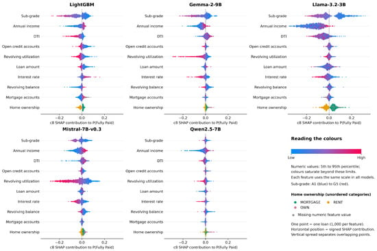
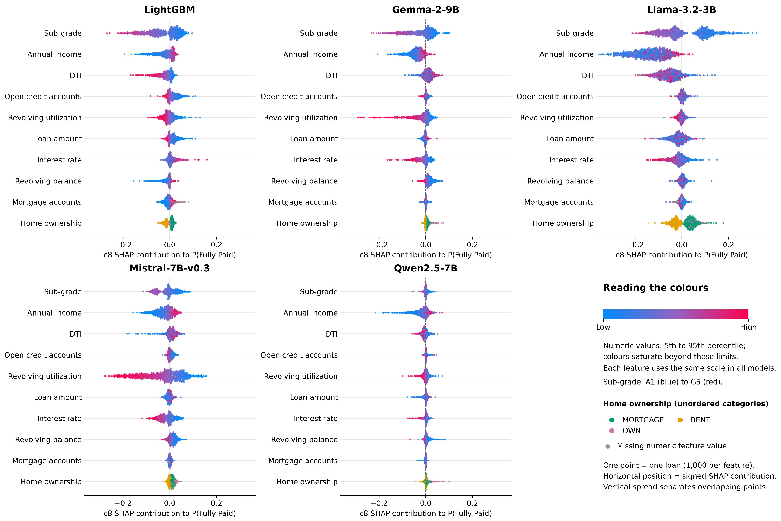
Figure 6 displays the signed c8 attribution distributions for the same benchmark-selected features, with individual loans colored by their observed feature values. Common inclusion in the top ten does not imply common direction or scale: the panels show marked model-specific differences, considered next.

Figure 6. Eight-cycle SHAP summary plots for LightGBM’s ten highest-ranked features on the common 1000-loan audit sample. Each point represents one loan’s signed contribution to predicted $P\left(\mathit{FullyPaid}\right)$; vertical spread separates overlapping points. Blue to red denotes low to high feature values, with numeric color limits at each feature’s 5th and 95th sample percentiles and saturation beyond these limits; gray denotes missing values. Sub-grade colors follow the ordinal scale A1 (blue) to G5 (red); home ownership uses a separate categorical legend because its levels are unordered. All panels share the same horizontal scale, feature order, and per-feature color mapping; dashed vertical lines mark zero.

4.4. SHAP Feature Dependence and Elicited LLM Feature Directions

Table 6 extends the directional comparison to the benchmark-defined top ten. Of the nine assessable features, agreement between each LLM’s single elicited global direction and its c8 SHAP direction is 6/9 (66.7%) for Gemma-2-9B, 4/9 (44.4%) for Llama-3.2-3B, and 3/9 (33.3%) for both Mistral-7B-v0.3 and Qwen2.5-7B. Home ownership is retained because it ranks tenth for LightGBM, but is not scored directionally because its categories are unordered. These rates quantify feature-level self-explanation faithfulness under our directional criterion; the remaining assessable features exhibit self-explanation unfaithfulness. They do not measure loan-level explanation quality or reveal internal reasoning.

Table 6. Elicited/SHAP direction for LightGBM’s ten highest-ranked features. In each cell, the first symbol is the LLM’s separately elicited context-free direction and the second is the empirical c8 SHAP direction: + positive, − negative, 0 neutral/weak, and NA not assessed. Bold cells agree. SHAP direction uses the prespecified Spearman threshold $\left|\rho \right|>0.10$.

Feature	Gemma-2-9B	Llama-3.2-3B	Mistral-7B-v0.3	Qwen2.5-7B
Sub-grade	$(+,-)$	$(+,-)$	$(-,-)$	$(+,-)$
Annual income	$(+,+)$	$(+,+)$	$(+,+)$	$(+,+)$
DTI	$(-,+)$	$(+,-)$	$(-,+)$	$(+,-)$
Open credit accounts	$(-,-)$	$(-,-)$	$(0,-)$	$(+,-)$
Revolving utilization	$(-,-)$	$(-,-)$	$(+,-)$	$(+,-)$
Loan amount	$(+,+)$	$(-,+)$	$(-,+)$	$(+,+)$
Interest rate	$(-,-)$	$(+,-)$	$(+,-)$	$(+,-)$
Revolving balance	$(-,-)$	$(-,-)$	$(+,-)$	$(+,-)$
Mortgage accounts	$(+,-)$	$(+,-)$	$(0,0)$	$(+,+)$
Home ownership	$(+,\mathrm{NA})$	$(+,\mathrm{NA})$	$(+,\mathrm{NA})$	$(+,\mathrm{NA})$
Agreement	6/9	4/9	3/9	3/9

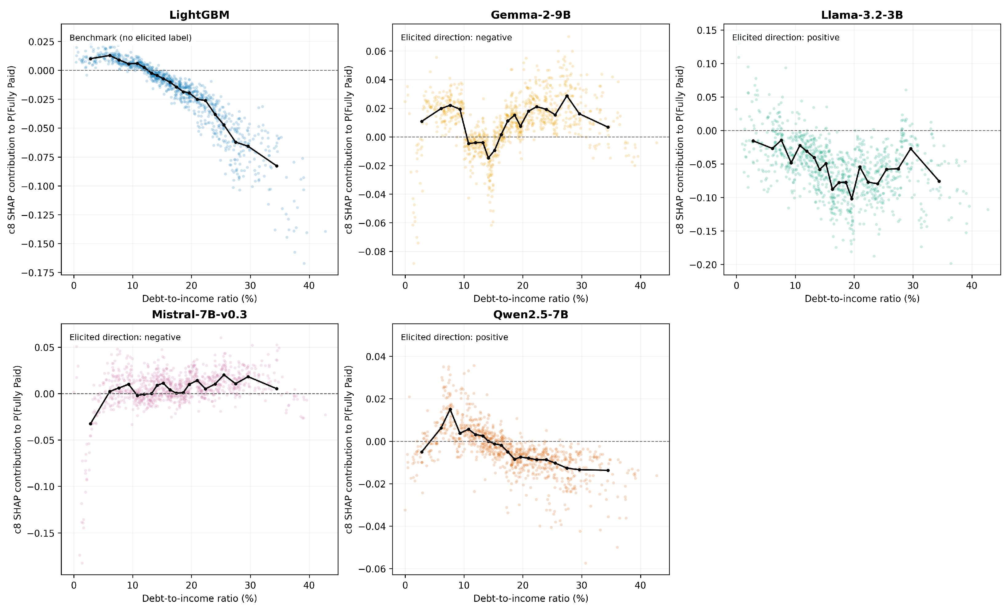
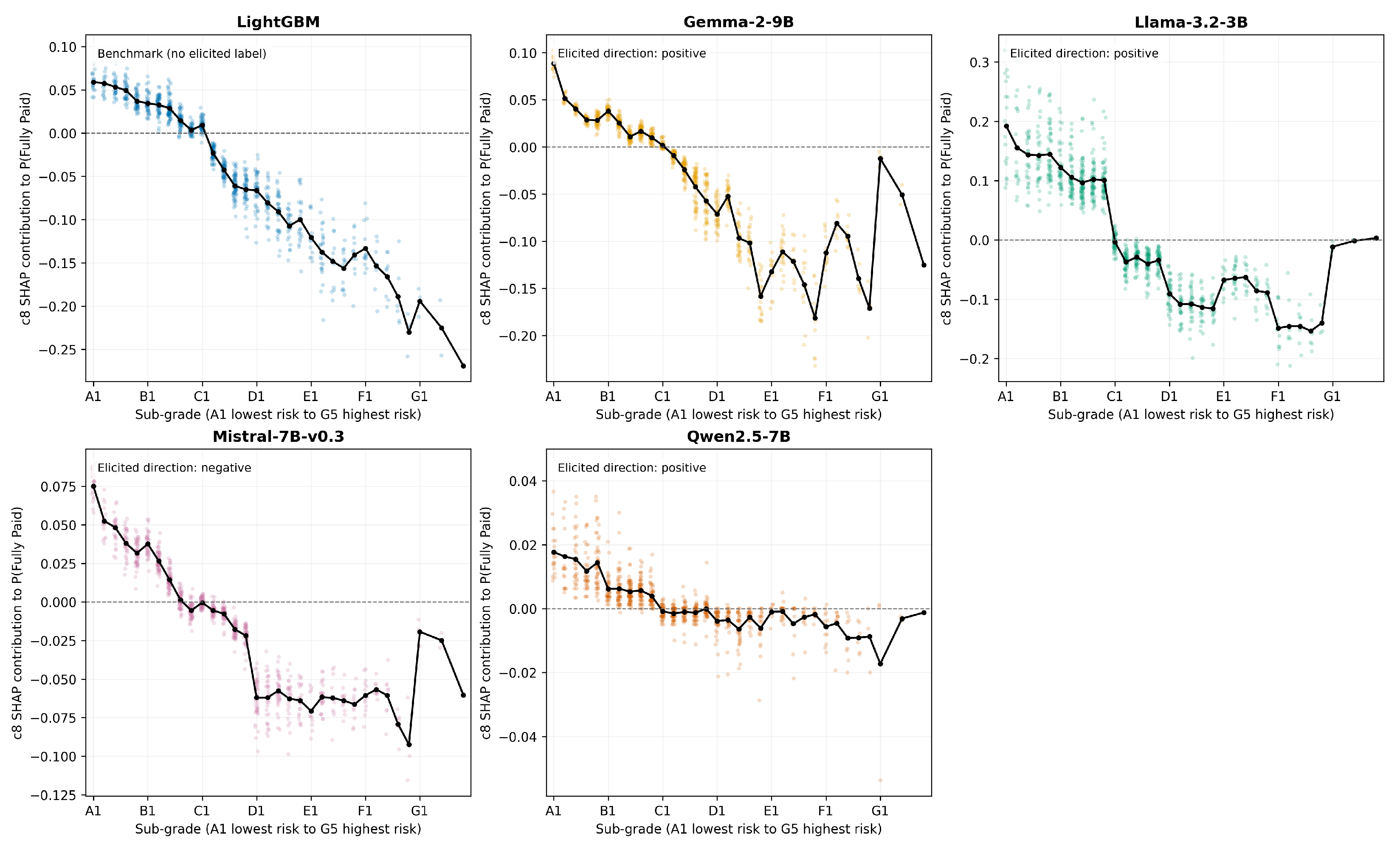
Several patterns show why direct empirical auditing is needed. Higher Annual income has a positive c8 SHAP direction for every model and agrees with every elicited label. By contrast, Interest rate is positive for LightGBM but negative for all four LLMs; only Gemma’s elicited negative label describes its own SHAP direction. All four DTI labels disagree with their respective SHAP directions (Figure 7): contributions decline with DTI for Llama-3.2-3B and Qwen2.5-7B, but increase overall for Gemma-2-9B and Mistral-7B-v0.3. For Sub-grade (Figure 8), all five empirical patterns decline as risk rises from A1 to G5, yet only Mistral supplies the corresponding negative label.

Figure 7. Eight-cycle SHAP dependence for debt-to-income ratio (DTI) on the common audit sample. The horizontal axis is DTI in percent, and the vertical axis is contribution to predicted $P\left(\mathit{FullyPaid}\right)$. The black line joins within-bin medians and is a descriptive overlay, not smoothing or partial dependence. Each LLM panel also reports the model’s one separately elicited global direction, which was obtained without a loan record.

Figure 8. Eight-cycle SHAP dependence for LendingClub sub-grade, ordered from A1 (lowest risk) to G5 (highest risk), on the common audit sample. The vertical axis is contribution to predicted $P\left(\mathit{FullyPaid}\right)$. Horizontal jitter separates overlapping observations and the black line joins category means. No partial-dependence estimate or smoothing is shown. Each LLM panel reports its one separately elicited global direction, obtained without a loan record.

The DTI and sub-grade panels are worked examples rather than the scope of the audit: the complete ten-feature comparison is in Table 6, and machine-readable results retain all 21 features. SHAP remains an operational description of behavior under the chosen masker, not a causal explanation. A mismatched global label demonstrates self-explanation unfaithfulness under the stated directional criterion. Nonlinearity or the inadequacy of a context-free sign may contribute to the mismatch; this finding does not identify the model’s internal mechanism.

5. Discussion

5.1. Implications for Credit-Risk Management Practice

Three practical lessons emerge from our audit. First, a standard gradient boosting pipeline remains clearly preferable to the evaluated zero-shot LLMs for structured retail credit data. LightGBM exceeded the best-discriminating LLM, Gemma-2-9B, by 0.0547 ROC-AUC and 0.0275 PR-AUC, while also reducing Brier score by 0.0627; all paired differences were statistically significant after multiplicity correction. The equal-weight LightGBM–Gemma ensemble was also worse than LightGBM alone on all three metrics. Institutions with access to labeled data and data science capacity therefore have little performance-based reason to substitute these LLMs for validated classical scorecards or GBDT models. Second, zero-shot inference avoids task-specific fitting, but this experiment does not test suitability for small-data or cold-start deployment. Gemma-2-9B achieved ROC-AUC 0.6693 and PR-AUC 0.8799 on the historical random holdout, but its Brier score of 0.2038 and visibly imperfect calibration rule out treating its numerical probabilities as validated risk estimates. Third, the c4/c8 experiment shows why attribution budgets must be reported: importance ranks and top-10 membership are stable, but small magnitude and distribution changes remain statistically detectable.

5.2. Regulatory Compliance and Model Governance

The divergences we document are directly relevant to model governance. Creditworthiness assessment is classified as high-risk AI under the EU AI Act, with obligations of transparency, traceability, and human oversight (European Parliament and Council, 2024), and supervisory frameworks such as SR 11-7, the OCC model risk handbook, and the EBA loan origination guidelines require that a model’s conceptual soundness be demonstrated and independently validated (Board of Governors of the Federal Reserve System, 2011; European Banking Authority, 2020; Office of the Comptroller of the Currency, 2021). Our results identify two specific patterns that such validation should examine for LLM-based credit models. First, the models exhibit different empirical directions: all four LLM SHAP patterns associate higher interest rates with lower repayment probability, whereas the LightGBM pattern shows the opposite association in this sample. A validator relying only on an assumed economic direction would miss this reversal without an empirical attribution check. Second, we observe self-explanation unfaithfulness, where the self-explanation is the one-off, context-free response to the feature-direction question: every LLM’s global DTI label disagrees with its empirical c8 SHAP direction, including negative labels from Gemma-2-9B and Mistral-7B-v0.3 despite their positive overall dependence patterns. These mismatches establish the unfaithfulness of the feature-direction self-explanations under our empirical criterion, without implying access to an internal mechanism or a loan-level rationale. The limited expressiveness of a context-free sign may contribute to the disagreement, but the elicited self-explanation still fails to match the measured direction. SHAP-style audits should therefore test such self-explanations against empirical, value-dependent attribution patterns in compliance documentation, in line with risk management guidance from NIST and ISO (International Organization for Standardization, 2023; National Institute of Standards and Technology, 2023) and with transparency practices such as model cards (Mitchell et al., 2019).

5.3. Limitations and Future Research

Several limitations qualify our findings and define an agenda for future work. First, the analysis relies on a single, historical U.S.-based peer-to-peer lending dataset; replication on bank loan books, SME portfolios, corporate distress data, and more recent lending cohorts would test the generality of the observed divergences. Second, our random-holdout design deliberately targets a pooled cross-sectional, in-distribution comparison under the assumption that individual loan records are exchangeable. This design is suitable for holding the evaluation distribution fixed while comparing model families, but it does not measure robustness to changes in underwriting policy, borrower composition, regulation, or macroeconomic conditions across origination cohorts. The results therefore should not be interpreted as evidence of future-cohort performance; a separate out-of-time validation would be required before prospective deployment. Third, the SHAP audit uses one fixed subsample and masker configuration. The nested c4 comparison gives essentially identical importance ranks and top-10 membership, but the small, statistically detectable magnitude and distribution changes show that numerical convergence is not complete; additional samples, maskers, and permutation budgets would be needed to quantify attribution uncertainty more broadly. Fourth, we examined four open-source instruction-tuned models in the 3B to 9B parameter range under one fixed zero-shot prompt; larger frontier models, alternative prompts, few-shot prompting, and parameter-efficient fine-tuning may narrow the performance gap and change the observed attribution patterns. Fifth, the calibration results apply to raw outputs under this fixed prompt. We did not test supervised post-hoc calibration, which would require a separate calibration sample and would no longer constitute a wholly zero-shot prediction pipeline. Sixth, the self-explanation faithfulness claim is specific to the one-off, context-free feature-direction response and its agreement with the empirical SHAP direction under the chosen masker and threshold. These self-explanations contain no instance-level or free-text rationale, cannot represent nonlinear effects fully, and cannot support conclusions about internal reasoning. These limitations bound the interpretation of the observed unfaithfulness rather than remove the claim. Seventh, our audit did not evaluate fairness: extending the framework with group fairness metrics over protected or proxy attributes is an important next step given the discrimination risks inherent in credit scoring. Taken together, these design boundaries mean that the study does not establish predictive performance, fairness, stability, or regulatory compliance for contemporary bank underwriting or for jurisdictions and populations outside the historical U.S. LendingClub setting. Finally, future work should explore hybrid designs in which LLMs process unstructured borrower information alongside classical models for structured data, together with out-of-time, external-validity, calibration, and fairness assessments.

6. Conclusions

The growing adoption of large language models for structured classification raises critical questions about their validity and safety in high-stakes financial decision-making. This study systematically compared zero-shot LLM classifiers with LightGBM on a structured loan default prediction task, evaluating both predictive performance and explainability through SHAP-based audits.

Our findings reveal that the LLMs overlap only partly with LightGBM’s attribution profile and remain inferior in predictive performance. LightGBM achieved the highest ROC-AUC and PR-AUC and the lowest Brier score; every paired LLM comparison favored LightGBM after multiplicity correction. The probability analysis also shows why discrimination and probability reliability must be assessed separately. Qwen2.5-7B produced the best LLM Brier score (0.1548, just below the 0.1580 constant-prevalence reference) despite its weakest ranking performance, whereas Gemma-2-9B ranked best among LLMs but had substantially larger raw probability error (Brier 0.2038). Each LLM shares six or seven of LightGBM’s top ten SHAP features, while agreement between its separately elicited directions and empirical SHAP directions is only 33–67% across the nine assessable top features. Four- and eight-cycle estimates preserve every LLM’s top-10 set and almost identical importance ranks, although small attribution-magnitude and distribution shifts are statistically detectable. The observed directional mismatches demonstrate self-explanation unfaithfulness: the self-explanations being tested are the one-off, context-free feature-direction responses. This claim concerns their agreement with empirical SHAP behavior, not loan-level rationales or internal reasoning. Moreover, the LightGBM–Gemma ensemble did not improve discrimination or Brier score, suggesting limited complementarity under the tested equal-weight design.

For credit-risk management, the message is twofold. LightGBM remains the more reliable choice when skilled data scientists and labeled data are available. Under the tested setup, the evaluated LLMs should be treated only as unvalidated challengers rather than substitutes for validated credit models; any proposed use, including in small-data or cold-start settings, would require independent validation of discrimination, calibration, stability, fairness, and decision patterns before operational deployment. More broadly, our results support treating probability validation, explainability audits, interpretable benchmarks, and human-in-the-loop oversight as preconditions, rather than afterthoughts, for deploying LLMs in credit risk and financial distress prediction. Future research should explore fine-tuned LLMs for tabular modeling, hybrid approaches that better integrate structured and unstructured information, and robust out-of-time, external-validity, reliability, and fairness assessments.

Appendix A.1. Sample Accounting and Output Validation

Table A1 distinguishes the common evaluation set from LightGBM’s internal model-selection sample. The internal split is class-stratified, with a 20% validation fraction and seed 42. Early stopping allows up to 2000 boosting rounds and stops after 100 rounds without improvement in validation ROC-AUC. The best internal ROC-AUC is 0.72384 at round 1650; the model is then refit for that many rounds on all 316,824 training loans. This validation score is a selection diagnostic, not an additional test-set performance estimate.

Table A1. Sample accounting and checks on the retained prediction records. Internal fit and validation rows partition the training set; the SHAP sample is a subset of the holdout.

Stage or Check	Count
Full study sample	396,030
LightGBM training partition/final refit	316,824
Internal fit/internal validation	253,459/63,365
Common holdout	79,206
Holdout Fully Paid/Charged Off	63,629/15,577
Holdout rows used for model selection	0
Valid aligned holdout probabilities, per LLM	79,206
Missing/duplicate holdout row identifiers, per LLM	0/0
Invalid holdout probabilities/prompt–row mismatches, per LLM	0/0
Common SHAP audit loans	1000
Distinct SHAP prediction prompts, per LLM	1,069,595
Strictly valid SHAP probability responses, per LLM	1,069,595
SHAP responses requiring format repair, per LLM	0

Table A1. Sample accounting and checks on the retained prediction records. Internal fit and validation rows partition the training set; the SHAP sample is a subset of the holdout.

Stage or Check	Count
Full study sample	396,030
LightGBM training partition/final refit	316,824
Internal fit/internal validation	253,459/63,365
Common holdout	79,206
Holdout Fully Paid/Charged Off	63,629/15,577
Holdout rows used for model selection	0
Valid aligned holdout probabilities, per LLM	79,206
Missing/duplicate holdout row identifiers, per LLM	0/0
Invalid holdout probabilities/prompt–row mismatches, per LLM	0/0
Common SHAP audit loans	1000
Distinct SHAP prediction prompts, per LLM	1,069,595
Strictly valid SHAP probability responses, per LLM	1,069,595
SHAP responses requiring format repair, per LLM	0

Each holdout prediction was checked against the same loan’s feature record and outcome; missing, duplicate, invalid, or mismatched records would stop evaluation rather than create a model-specific subset. The SHAP prompt counts include perturbed feature combinations, not additional observed loans. For each of the four primary LLMs, all retained SHAP responses satisfied the single-probability schema without format repair or probability imputation. These are checks of retained outputs, not counts of service retries or failed requests.

Appendix A.2. Calibration and Paired Performance Inference

Table A2 reports overall mean probabilities and ECE, together with the most populated reliability bin for each model. The observed holdout repayment rate is 0.8033 for every model. The displayed bin is selected solely by its support; it is an intermediate coordinate of Figure 3, not a separate evaluation sample. Bins are $[0,0.1),\dots ,[0.9,1]$; empty bins contribute zero to ECE and have no plotted rate. All ten bins enter the ECE calculation. Within each nonempty bin, the plotted quantities are the arithmetic mean probability and the fraction of Fully Paid loans, with a 95% Wilson interval for the latter. A small ECE at this bin resolution does not establish fine-grained calibration or discrimination.

Table A2. Intermediate calibration summaries. $\overline{p}$ is the overall mean prediction; $n_k$, ${\overline{p}}_k$, and ${\overline{y}}_k$ describe the most populated bin. The ensemble is the equal mean of LightGBM and Gemma.

Model	$\overline{\mathit{p}}$	ECE	Largest Bin	${\mathit{n}}_{\mathit{k}}$	${\overline{\mathit{p}}}_{\mathit{k}}$	${\overline{\mathit{y}}}_{\mathit{k}}$
LightGBM	0.8034	0.0016	$[0.8,0.9)$	27,172	0.8544	0.8562
Gemma-2-9B	0.6040	0.1994	$[0.6,0.7)$	26,493	0.6479	0.8028
Llama-3.2-3B	0.4988	0.3045	$[0.8,0.9)$	29,197	0.8500	0.8764
Mistral-7B-v0.3	0.4908	0.3125	$[0.3,0.4)$	17,522	0.3499	0.7455
Qwen2.5-7B	0.7808	0.0226	$[0.7,0.8)$	55,836	0.7500	0.7686
Ensemble	0.7037	0.0996	$[0.7,0.8)$	22,241	0.7530	0.8383

Table A2. Intermediate calibration summaries. $\overline{p}$ is the overall mean prediction; $n_k$, ${\overline{p}}_k$, and ${\overline{y}}_k$ describe the most populated bin. The ensemble is the equal mean of LightGBM and Gemma.

Model	$\overline{\mathit{p}}$	ECE	Largest Bin	${\mathit{n}}_{\mathit{k}}$	${\overline{\mathit{p}}}_{\mathit{k}}$	${\overline{\mathit{y}}}_{\mathit{k}}$
LightGBM	0.8034	0.0016	$[0.8,0.9)$	27,172	0.8544	0.8562
Gemma-2-9B	0.6040	0.1994	$[0.6,0.7)$	26,493	0.6479	0.8028
Llama-3.2-3B	0.4988	0.3045	$[0.8,0.9)$	29,197	0.8500	0.8764
Mistral-7B-v0.3	0.4908	0.3125	$[0.3,0.4)$	17,522	0.3499	0.7455
Qwen2.5-7B	0.7808	0.0226	$[0.7,0.8)$	55,836	0.7500	0.7686
Ensemble	0.7037	0.0996	$[0.7,0.8)$	22,241	0.7530	0.8383

For the paired bootstrap (seed 42), each of the 2000 replicates samples 63,629 Fully Paid and 15,577 Charged Off loans with replacement, carrying all predictions with each sampled outcome. For a metric difference ${\Delta }_b$ (comparator minus LightGBM), the reported two-sided sign-tail value is

$$p=min\left\{1,2min\left[{\displaystyle \frac{1+{\sum }_{b=1}^B\mathbf{1}({\Delta }_b\le 0)}{B+1}},{\displaystyle \frac{1+{\sum }_{b=1}^B\mathbf{1}({\Delta }_b\ge 0)}{B+1}}\right]\right\},B=2000.$$

(A1)

The smallest attainable raw value is therefore $2/2001=0.0009995$. All five comparisons reach this bound for each metric; Holm adjustment within each five-comparison family gives $10/2001=0.0049975$, explaining the common rounded value of 0.005 in Table 3. These identical reported values reflect finite resampling resolution, not identical effect sizes. The percentile intervals retain the magnitude information. The constant-prevalence Brier reference uses the observed holdout prevalence and is a descriptive reference, not a separately trained forecast.

Appendix A.3. SHAP Construction, Sensitivity, and Direction Classification

The 1000 audit loans are sampled without replacement from the holdout with sampling seed 0. Categorical predictors are label-encoded for masking; the five background representatives are obtained by applying SHAP’s k-means summary to the encoded holdout predictors, without outcomes. The centroid matrix is passed as the common background, so the five representatives receive equal weight in masking. Masked categorical values are mapped back to the model input representation. This is a marginal replacement scheme: it does not estimate the conditional distribution of missing features and can produce combinations that do not occur in observed loans. Consequently, correlated predictors and the numerical encoding used to construct the background can affect the attributions.

For audit position $i=0,\dots ,999$, permutation seed $42+i$ is used for both budgets. A cycle traverses a random feature ordering and its reverse. The four-cycle run repeats the initial part of the eight-cycle design, preserving the rows, background, and initial randomization. The maximum difference between reconstructed local predictions (base value plus summed SHAP values) across these budgets is below $4\times {10}^{-16}$ for every LLM. This verifies agreement of the reconstructed output, not convergence of individual feature contributions.

For loan i and cycle budget c, the magnitude statistic is $m_i^{\left(c\right)}={21}^{-1}{\sum }_{j=1}^{21}\left|{\varphi }_{ij}^{\left(c\right)}\right|$. The paired two-sided Wilcoxon signed-rank test compares the 1000 paired magnitudes using its normal approximation. Table A3 reports their means and raw p-values; the percentage changes and adjusted results appear in Table 5.

Table A3. Intermediate inputs to the SHAP cycle-budget comparison. Mean magnitudes are in probability units. Grid size is the number of distinct pooled quantiles used for the distribution comparison.

Model	Mean ${\mathit{m}}^{\left(4\right)}$	Mean ${\mathit{m}}^{\left(8\right)}$	Raw Wilcoxon p	Grid Size
Gemma-2-9B	0.017273	0.017085	$2.30\times {10}^{-10}$	83
Llama-3.2-3B	0.038327	0.036931	$4.31\times {10}^{-47}$	85
Mistral-7B-v0.3	0.016836	0.016427	$1.18\times {10}^{-42}$	86
Qwen2.5-7B	0.007564	0.007354	$1.58\times {10}^{-19}$	53

Table A3. Intermediate inputs to the SHAP cycle-budget comparison. Mean magnitudes are in probability units. Grid size is the number of distinct pooled quantiles used for the distribution comparison.

Model	Mean ${\mathit{m}}^{\left(4\right)}$	Mean ${\mathit{m}}^{\left(8\right)}$	Raw Wilcoxon p	Grid Size
Gemma-2-9B	0.017273	0.017085	$2.30\times {10}^{-10}$	83
Llama-3.2-3B	0.038327	0.036931	$4.31\times {10}^{-47}$	85
Mistral-7B-v0.3	0.016836	0.016427	$1.18\times {10}^{-42}$	86
Qwen2.5-7B	0.007564	0.007354	$1.58\times {10}^{-19}$	53

The distribution statistic is the maximum absolute empirical CDF difference evaluated at the distinct pooled c4/c8 quantiles from 0.01 to 0.99 in steps of 0.01. Thus, it is a grid-based maximum, not the unrestricted Kolmogorov–Smirnov statistic. For each of 10,000 randomizations, the c4/c8 labels are swapped within each loan, keeping its 21 contributions together; the statistic is recomputed on the fixed grid. Seeds 42–45 correspond to Gemma, Llama, Mistral, and Qwen. The randomization p-value is (1 + number of statistics at least as large as observed)/10,001. All four models reach their lower bound, $1/\mathrm{10,001}$; Holm adjustment gives $4/\mathrm{10,001}\simeq 0.000400$. Multiplicity correction is separate for the magnitude and distribution families. The paired construction preserves within-loan feature dependence; it does not test robustness to different audit samples or backgrounds.

Correlations use the observed feature values and the same model’s eight-cycle SHAP contributions, retaining finite pairs. Numerical features keep their natural scale, sub-grade is ordered A1 through G5, and ties receive average ranks. Direction labels use the unrounded correlations, not a significance test; neutral/weak is matched to an elicited neutral response. For example, Table A4 makes the opposite empirical DTI signs visible, while Table 6 supplies the independently elicited labels needed to identify disagreement.

Table A4. Spearman correlations underlying the empirical direction labels in Table 6. Rows follow LightGBM’s c8 importance ranking. Positive: $\rho >0.10$; negative: $\rho <-0.10$; otherwise neutral/weak. Unordered home ownership is not assessed.

Feature	Gemma	Llama	Mistral	Qwen
Sub-grade	$-0.968$	$-0.906$	$-0.960$	$-0.828$
Annual income	$+0.872$	$+0.426$	$+0.913$	$+0.853$
DTI	$+0.240$	$-0.389$	$+0.311$	$-0.706$
Open credit accounts	$-0.807$	$-0.103$	$-0.686$	$-0.558$
Revolving utilization	$-0.969$	$-0.455$	$-0.987$	$-0.856$
Loan amount	$+0.476$	$+0.148$	$+0.112$	$+0.432$
Interest rate	$-0.959$	$-0.706$	$-0.910$	$-0.655$
Revolving balance	$-0.767$	$-0.335$	$-0.818$	$-0.745$
Mortgage accounts	$-0.454$	$-0.356$	$-0.098$	$+0.285$
Home ownership	—	—	—	—

Table A4. Spearman correlations underlying the empirical direction labels in Table 6. Rows follow LightGBM’s c8 importance ranking. Positive: $\rho >0.10$; negative: $\rho <-0.10$; otherwise neutral/weak. Unordered home ownership is not assessed.

Feature	Gemma	Llama	Mistral	Qwen
Sub-grade	$-0.968$	$-0.906$	$-0.960$	$-0.828$
Annual income	$+0.872$	$+0.426$	$+0.913$	$+0.853$
DTI	$+0.240$	$-0.389$	$+0.311$	$-0.706$
Open credit accounts	$-0.807$	$-0.103$	$-0.686$	$-0.558$
Revolving utilization	$-0.969$	$-0.455$	$-0.987$	$-0.856$
Loan amount	$+0.476$	$+0.148$	$+0.112$	$+0.432$
Interest rate	$-0.959$	$-0.706$	$-0.910$	$-0.655$
Revolving balance	$-0.767$	$-0.335$	$-0.818$	$-0.745$
Mortgage accounts	$-0.454$	$-0.356$	$-0.098$	$+0.285$
Home ownership	—	—	—	—

The recorded analysis environment uses Python 3.11.15, NumPy 2.2.6, pandas 2.2.3, and LightGBM 4.6.0. Performance inference uses scikit-learn 1.6.1 and SciPy 1.15.2; the SHAP analysis uses SHAP 0.51.0, scikit-learn 1.5.2, and SciPy 1.17.1. These versions describe the statistical analysis environment, not a complete specification of the external inference service.

References

- Achiam, J., Adler, S., Agarwal, S., Ahmad, L., Akkaya, I., Aleman, F. L., Almeida, D., Altenschmidt, J., Altman, S., Anadkat, S., Avila, R., Babuschkin, I., Balaji, S., Balcom, V., Baltescu, P., Bao, H., Bavarian, M., Belgum, J., Bello, I., … Zoph, B. (2023). GPT-4 technical report. arXiv, arXiv:2303.08774. [Google Scholar]
- Bank of England and Financial Conduct Authority. (2022). Artificial intelligence public-private forum: Final report (Tech. Rep.). Bank of England and Financial Conduct Authority. Available online: https://www.bankofengland.co.uk/-/media/boe/files/fintech/ai-public-private-forum-final-report.pdf (accessed on 6 September 2026).
- Basel Committee on Banking Supervision. (2017). Basel iii: Finalising post-crisis reforms (Tech. Rep.). Bank for International Settlements. Available online: https://www.bis.org/bcbs/publ/d424.htm (accessed on 6 September 2026).
- Board of Governors of the Federal Reserve System. (2011). Supervisory guidance on model risk management (sr 11-7). Available online: https://www.federalreserve.gov/boarddocs/srletters/2011/sr1107.pdf (accessed on 6 September 2026).
- Boughaci, D., & Alkhawaldeh, A. A. K. (2020). Appropriate machine learning techniques for credit scoring and bankruptcy prediction in banking and finance: A comparative study. Risk and Decision Analysis, 8(1–2), 15–24. [Google Scholar] [CrossRef] [Scilit]
- Brown, T. B., Mann, B., Ryder, N., Subbiah, M., Kaplan, J. D., Dhariwal, P., Neelakantan, A., Shyam, P., Sastry, G., Askell, A., Agarwal, S., Herbert-Voss, A., Krueger, G., Henighan, T., Child, R., Ramesh, A., Ziegler, D., Wu, J., Winter, C., … Amodei, D. (2020). Language models are few-shot learners. Advances in Neural Information Processing Systems, 33, 1877–1901. [Google Scholar]
- Buckmann, M., & Hill, E. (2024). Logistic Regression makes small LLMs strong and explainable “tens-of-shot” classifiers. arXiv, arXiv:2408.03414. [Google Scholar]
- Bussmann, N., Giudici, P., Marinelli, D., & Papenbrock, J. (2021). Explainable machine learning in credit risk management. Computational Economics, 57(1), 203–216. [Google Scholar] [CrossRef] [Scilit]
- Chen, C., Yu, J., Chen, S., Liu, C., Wan, Z., Zhou, S., Luo, Y., Zhang, R., Bitterman, D., Wang, F., & Shu, K. (2024). ClinicalBench: Can LLMs beat traditional ML models in clinical prediction? arXiv, arXiv:2411.06469. [Google Scholar]
- Chen, T., & Guestrin, C. (2016, August 13–17). XGBoost: A scalable tree boosting system. 22nd ACM SIGKDD International Conference on Knowledge Discovery and Data Mining (pp. 785–794), San Francisco, CA, USA. [Google Scholar]
- Černevičienė, J., & Kabašinskas, A. (2024). Explainable artificial intelligence (XAI) in Finance: A systematic literature review. Artificial Intelligence Review, 57(8), 216. [Google Scholar] [CrossRef] [Scilit]
- Dehghanighobadi, Z., Fischer, A., & Zafar, M. B. (2025). Can LLMs explain themselves counterfactually? arXiv, arXiv:2502.18156. [Google Scholar]
- Doshi-Velez, F., & Kim, B. (2017). Towards a rigorous science of interpretable machine learning. arXiv, arXiv:1702.08608. [Google Scholar]
- European Banking Authority. (2020). Guidelines on loan origination and monitoring (eba/gl/2020/06). Available online: https://www.eba.europa.eu/activities/single-rulebook/regulatory-activities/credit-risk/guidelines-loan-origination-and-monitoring (accessed on 6 September 2026).
- European Parliament and Council. (2024). Regulation (eu) 2024/1689—Artificial intelligence act. Available online: https://eur-lex.europa.eu/legal-content/EN/TXT/PDF/?uri=OJ:L_202401689 (accessed on 6 September 2026).
- European Union. (2016). Regulation (eu) 2016/679 of the european parliament and of the council of 27 april 2016 on the protection of natural persons with regard to the processing of personal data and on the free movement of such data, and repealing directive 95/46/ec (general data protection regulation) (No. 119). Available online: https://eur-lex.europa.eu/eli/reg/2016/679/oj/eng (accessed on 6 September 2026).
- Fang, X., Xu, W., Tan, F. A., Zhang, J., Hu, Z., Qi, Y., Nickleach, S., Socolinsky, D., Sengamedu, S., & Faloutsos, C. (2024). Large language models (LLMs) on tabular data: Prediction, generation, and understanding—A survey. arXiv, arXiv:2402.17944. [Google Scholar]
- Gebru, T., Morgenstern, J., Vecchione, B., Vaughan, J. W., Wallach, H., Daumé, H., III, & Crawford, K. (2021). Datasheets for datasets. Communications of the ACM, 64(12), 86–92. [Google Scholar] [CrossRef] [Scilit]
- Gemma Team, Riviere, M., Pathak, S., Sessa, P. G., Hardin, C., Bhupatiraju, S., Hussenot, L., Mesnard, T., Shahriari, B., Ramé, A., Ferret, J., Liu, P., Tafti, P., Friesen, A., Casbon, M., Ramos, S., Kumar, R., Le Lan, C., Jerome, S., … Andreev, A. (2024). Gemma 2: Improving open language models at a practical size. arXiv, arXiv:2408.00118. [Google Scholar]
- Ghaffarzadeh-Esfahani, M., Ghaffarzadeh-Esfahani, M., Salahi-Niri, A., Toreyhi, H., Atf, Z., Mohsenzadeh-Kermani, A., Sarikhani, M., Tajabadi, Z., Shojaeian, F., Bagheri, M. H., Feyzi, A., Tarighat-Payma, M., Gazmeh, N., Heydari, F., Afshar, H., Allahgholipour, A., Alimardani, F., Salehi, A., Asadimanesh, N., … Safavi-Naini, S. A. A. (2024). Large language models versus classical machine learning: Performance in COVID-19 mortality prediction using high-dimensional tabular data. arXiv, arXiv:2409.02136. [Google Scholar]
- Hegselmann, S., Buendia, A., Lang, H., Agrawal, M., Jiang, X., & Sontag, D. (2023, July 23–29). TabLLM: Few-shot classification of tabular data with large language models. 40th International Conference on Machine Learning (ICML), Honolulu, HI, USA. [Google Scholar]
- Huang, S., Mamidanna, S., Jangam, S., Zhou, Y., & Gilpin, L. H. (2023). Can large language models explain themselves? A study of LLM-generated self-explanations. arXiv, arXiv:2310.11207. [Google Scholar]
- International Organization for Standardization. (2023). Information technology—Artificial intelligence—Guidance on risk management (ISO/IEC 23894:2023). Available online: https://www.iso.org/standard/77304.html (accessed on 6 September 2026).
- Jiang, A. Q., Sablayrolles, A., Mensch, A., Bamford, C., Chaplot, D. S., de las Casas, D., Bressand, F., Lengyel, G., Lample, G., Saulnier, L., Renard Lavaud, L., Lachaux, M.-A., Stock, P., Le Scao, T., Lavril, T., Wang, T., Lacroix, T., & El Sayed, W. (2023). Mistral-7B. arXiv, arXiv:2310.06825. [Google Scholar]
- Ke, G., Meng, Q., Finley, T., Wang, T., Chen, W., Ma, W., Ye, Q., & Liu, T. (2017). LightGBM: A highly efficient gradient boosting decision tree. Advances in Neural Information Processing Systems, 30, 3146–3154. [Google Scholar]
- Lundberg, S. M., & Lee, S. (2017). A unified approach to interpreting model predictions. Advances in Neural Information Processing Systems (NeurIPS), 30, 4765–4774. [Google Scholar]
- Madaan, M., Kumar, A., Keshri, C., Jain, R., & Nagrath, P. (2021). Loan default prediction using decision trees and random forest: A comparative study. In IOP Conference Series: Materials Science and Engineering (Vol. 1022, p. 012042). IOP Publishing. [Google Scholar]
- Martins, T., De Almeida, A. M., Cardoso, E., & Nunes, L. (2023). Explainable artificial intelligence (XAI): A systematic literature review on taxonomies and applications in Finance. IEEE Access, 12, 618–629. [Google Scholar] [CrossRef] [Scilit]
- Meta AI. (2024). Llama 3.2: Revolutionizing edge AI and vision with open, customizable models. Available online: https://ai.meta.com/blog/llama-3-2-connect-2024-vision-edge-mobile-devices/ (accessed on 6 September 2026).
- Misheva, B. H., Osterrieder, J., Hirsa, A., Kulkarni, O., & Lin, S. F. (2021). Explainable AI in credit risk management. arXiv, arXiv:2103.00949. [Google Scholar]
- Mitchell, M., Wu, S., Zaldivar, A., Barnes, P., Vasserman, L., Hutchinson, B., Spitzer, E., Raji, I. D., & Gebru, T. (2019). Model cards for model reporting. In Proceedings of the conference on fairness, accountability, and transparency (FAT*) (pp. 220–229). Association for Computing Machinery. Available online: https://dl.acm.org/doi/10.1145/3287560.3287596 (accessed on 6 September 2026).
- National Institute of Standards and Technology. (2023). Artificial intelligence risk management framework (AI RMF 1.0) (Tech. Rep. No. NIST AI 100-1). National Institute of Standards and Technology. Available online: https://nvlpubs.nist.gov/nistpubs/ai/nist.ai.100-1.pdf (accessed on 6 September 2026).
- Office of the Comptroller of the Currency. (2021, August). Model Risk Management, Comptroller’s Handbook. Version 1.0. Available online: https://www.occ.gov/news-issuances/bulletins/2021/bulletin-2021-39.html (accessed on 6 September 2026).
- Sarkar, A. (2024). Large language models cannot explain themselves. arXiv, arXiv:2405.04382. [Google Scholar]
- Shi, Z., Kim, J., Jeong, D., & Pfister, H. (2024). Surprisingly simple: Large language models are zero-shot feature extractors for tabular and text data. arXiv, arXiv:2409.00079. [Google Scholar]
- Song, X., & Bahri, D. (2025). Decoding-based regression. arXiv, arXiv:2501.19383. [Google Scholar]
- Song, X., Li, O., Lee, C., Yang, B., Peng, D., Perel, S., & Chen, Y. (2024). Omnipred: Language models as universal regressors. arXiv, arXiv:2402.14547. [Google Scholar]
- Srinivasa Rao, M., Sekhar, C., & Bhattacharyya, D. (2021). Comparative analysis of machine learning models on loan risk analysis. In Machine intelligence and soft computing: Proceedings of ICMISC 2020 (pp. 81–90). Springer. [Google Scholar]
- Turpin, M., Michael, J., Perez, E., & Bowman, S. (2023). Language models don’t always say what they think: Unfaithful explanations in chain-of-thought prompting. Advances in Neural Information Processing Systems, 36, 74952–74965. [Google Scholar] [CrossRef] [Scilit]
- Vacareanu, R., Negru, V.-A., Suciu, V., & Surdeanu, M. (2024). From words to numbers: Your large language model is secretly a capable regressor when given in-context examples. arXiv, arXiv:2404.07544. [Google Scholar]
- Vaswani, A., Shazeer, N., Parmar, N., Uszkoreit, J., Jones, L., Gomez, A. N., Kaiser, Ł., & Polosukhin, I. (2017). Attention is all you need. Advances in Neural Information Processing Systems (NeurIPS), 30, 5998–6008. [Google Scholar]
- Wei, J., Wang, X., Schuurmans, D., Bosma, M., Ichter, B., Xia, F., Chi, E., Le, Q., & Zhou, D. (2022). Chain-of-thought prompting elicits reasoning in large language models. Advances in Neural Information Processing Systems, 35, 24824–24837. [Google Scholar] [CrossRef] [Scilit]
- Wolf, T., Debut, L., Sanh, V., Chaumond, J., Delangue, C., Moi, A., Cistac, P., Rault, T., Louf, R., Funtowicz, M., Davison, J., Shleifer, S., von Platen, P., Ma, C., Jernite, Y., Plu, J., Xu, C., Le Scao, T., Gugger, S., … Rush, A. M. (2020). Transformers: State-of-the-art natural language processing. In Proceedings of the 2020 conference on empirical methods in natural language processing: System demonstrations (pp. 38–45). Association for Computational Linguistics. [Google Scholar]
- Yang, A., Yang, B., Zhang, B., Hui, B., Zheng, B., Yu, B., Li, C., Liu, D., Huang, F., Wei, H., Lin, H., Yang, J., Tu, J., Zhang, J., Yang, J., Yang, J., Zhou, J., Lin, J., Dang, K., … Qiu, Z. (2024). Qwen2.5 technical report. arXiv, arXiv:2412.15115. [Google Scholar]
Disclaimer/Publisher’s Note: The statements, opinions and data contained in all publications are solely those of the individual author(s) and contributor(s) and not of MDPI and/or the editor(s). MDPI and/or the editor(s) disclaim responsibility for any injury to people or property resulting from any ideas, methods, instructions or products referred to in the content. |
© 2026 by the authors. Licensee MDPI, Basel, Switzerland. This article is an open access article distributed under the terms and conditions of the Creative Commons Attribution (CC BY) license.