


Abstract
This paper develops a quantitative framework for climate–financial risk measurement that combines a spatially explicit jump–diffusion asset–loss model with prudentially aligned risk metrics. The approach connects regional physical hazards and transition variables derived from climate-consistent pathways to asset returns and credit parameters through the use of climate-adjusted volatilities and jump intensities. Fat tails and geographic heterogeneity are captured by it, which conventional diffusion-based or purely narrative stress tests fail to reflect. The framework delivers portfolio-level Spatial Climate Value-at-Risk (SCVaR) and Expected Shortfall (ES) across scenario–horizon matrices and incorporates an explicit robustness layer (block bootstrap confidence intervals, unconditional/conditional coverage backtests, and structural-stability tests). All ES measures are understood as Conditional Expected Shortfall (CES), i.e., tail expectations evaluated conditional on climate stress scenarios. Applications to bank loan books, pension portfolios, and sovereign exposures show how climate shocks reprice assets, alter default and recovery dynamics, and amplify tail losses in a region- and sector-dependent manner. The resulting, statistically validated outputs are designed to be decision-useful for Internal Capital Adequacy Assessment Process (ICAAP) and Pillar 2: climate-adjusted capital buffers, scenario-based stress calibration, and disclosure bridges that complement alignment metrics such as the Green Asset Ratio (GAR). Overall, the framework operationalises a move from exposure tallies to forward-looking, risk-sensitive, and auditable measures suitable for supervisory dialogue and internal risk appetite.
1. Introduction
Supervisors now expect banks to quantify and manage climate risk within the internal capital adequacy assessment process (ICAAP), risk-appetite frameworks, and stress-testing programmes. In the euro area, the European Central Bank’s Guide on climate-related and environmental risks sets explicit expectations to embed climate drivers into business strategy (Exp. 1–2), governance and risk-appetite (Exp. 3–6), risk management across risk types (Exp. 7), credit underwriting and monitoring (Exp. 8), market/operational/liquidity risk (Exp. 9–12), and disclosures (Exp. 13) (ECB, 2020). The ECB’s 2022 climate stress test (CST) further highlighted persistent data and methodology gaps—coverage of physical risks, treatment of tail events, limited spatial granularity, and weak links from narratives to capital metrics—underscoring the need for operational, statistically validated tools suitable for ICAAP and Pillar 2 processes (ECB, 2022). Global standard-setters echo this direction: the BCBS Principles call for measurement of climate risks as drivers of traditional risk categories and for decision-useful scenario analysis and stress testing for capital planning (BCBS, 2022).
Climate change poses systemic financial risks via physical channels (acute and chronic hazards such as floods, heatwaves, sea-level rise) and transition channels (policy, technology, and market shifts) (Campiglio et al., 2023; ECB, 2020; Feng & Chen, 2025; Redondo & Aracil, 2024). A large literature spans scenario analysis and stress testing, sensitivity analysis, and exposure-based metrics such as Weighted Average Carbon Intensity (WACI), (Climate) VaR, and Climate Risk Capital Shortfall (CRISK) (Battiston et al., 2021; Gualandri et al., 2024; Jung et al., 2025; Rogge, 2023; TCFD, 2017). Yet four practical limitations recur: (i) weak capture of non-linear, fat-tailed dynamics (Apostolou & Papaioannou, 2024); (ii) limited cross-jurisdictional harmonisation (BCBS, 2021); (iii) insufficient treatment of spatial heterogeneity (Kolozsi et al., 2022); and (iv) difficulties translating long-horizon climate pathways into forward-looking, capital-relevant risk measures (EBA, 2020; ECB, 2023). Recent surveys emphasise the lack of consensus on modelling approaches and the tendency of diffusion-only dynamics to smooth extreme, spatially heterogeneous shocks (Trotta et al., 2025), while granular studies show that climate-adjusted processes materially thicken loss tails and raise capital needs, with strong regional dispersion (Rania, 2025).
A unified Spatial Stress Testing and Climate Value-at-Risk (SCVaR) framework is developed to make climate risk measurement bank-usable for prudential purposes. Methodologically, a spatially explicit, hazard-linked jump–diffusion structure is embedded, estimated on financial and regional climate data, and both SCVaR and the coherent tail metric CES are computed. Implementation is provided in three complementary forms aligned with banks’ risk channels: (i) a market-based SCVaR via climate re-pricing of assets; (ii) a credit-portfolio SCVaR via scenario-to-PD/LGD mappings; and (iii) a hybrid SCVaR that jointly models market re-pricing and credit migration. All variants share a harmonised scenario set (NGFS Orderly/Disorderly/Hot-house world), near-term and medium-term horizons, and a spatial mapping from instruments to regional hazards (NGFS, 2021). A built-in robustness layer (bootstrap confidence intervals, coverage tests, stability/break tests, and sensitivity to hazard inputs and financed-emissions proxies) ensures statistical validation.
The framework delivers (a) tail-sensitive, portfolio-level metrics for risk-appetite calibration and ICAAP benchmarking; (b) stress-test outputs that are both scenario-consistent and model-validated; and (c) a transparent bridge from alignment-style disclosures (e.g., GAR) to risk-sensitive, capital-relevant measures. By quantifying spatial heterogeneity and fat-tail amplification, SCVaR addresses the gaps identified by the ECB CST and aligns with BCBS guidance on measurement and scenario analysis (BCBS, 2022; ECB, 2022).
The rest of the manuscript is organised as follows. Section 2 reviews the current approaches to climate-related financial risk measurement through a systematic survey of the literature and positions the contribution of the present framework. Section 3 details the econometric specification and estimation strategy, including the operationalization of market-based, credit-portfolio, and hybrid SCVaR implementations. Section 4 presents simulation-based results that illustrate the statistical properties of SCVaR under stylized climate stress scenarios. To establish empirical validity and practical feasibility, Section 5 introduces a real-world application based on publicly available financial and climate data, including sovereign bond returns, NGFS-consistent hazard indicators, and emissions intensity measures. This section documents the full data construction pipeline, parameter estimation of the jump–diffusion components, and a comparative evaluation of SCVaR and conditional expected shortfall against classical VaR benchmarks. Section 6 discusses supervisory and institutional applications, building on the empirically calibrated SCVaR measures, including ICAAP/Pillar 2 integration, stress-test calibration, and climate-risk disclosure. Section 7 synthesises the empirical and simulation evidence and discusses its implications for climate stress testing, capital planning, and supervisory practice, while Section 8 outlines policy-relevant avenues of intervention. Section 9 concludes the study.
2. Literature Review
To establish the state of the art in the measurement of climate-related financial risks and to position the contribution, a systematic literature review is carried out. Sources include central bank and supervisory publications, as well as peer-reviewed journals indexed in EconLit, Scopus, and Web of Science over the period from 2000 to 2025. Search terms combine climate-finance and risk-modelling keywords (e.g., “climate stress test”, “NGFS”, “climate VaR”, “expected shortfall”, “jump–diffusion”, “spatial hazards”, “credit migration”). Inclusion criteria require (i) explicit treatment of climate-related financial risks or supervisory stress testing; (ii) methodological content on VaR/ES, tail modelling, or validation; and (iii) application to banks, pensions, or sovereigns. Exclusions are non-financial climate studies without risk-modelling content and purely descriptive reports without methodological detail. References are screened for relevance and clustered into six strands to identify strengths, limitations, and gaps.
The results confirm that the measurement of climate-related financial risks spans qualitative scenario analysis, supervisory stress testing, market-based indicators, credit and collateral channels, econometric and structural models, and regulatory disclosure frameworks. Therefore, these strands are reviewed in a systematic manner, and their strengths and weaknesses are highlighted for each one. At the end, the positioning of this paper is summarised as completing an existing gap.
2.1. Scenario Analysis and Supervisory Stress Testing
Scenario analysis and climate stress testing are now standard among central banks and supervisors (ECB, 2020, 2022; EBA, 2020, 2025). Exercises typically rely on long-horizon pathways from the Network for Greening the Financial System (NGFS) (NGFS, 2021) and translate them into macro–sectoral trajectories to test portfolio resilience under transition and physical narratives (Gualandri et al., 2024; Rogge, 2023). The ECB’s 2022 CST and related work document the feasibility and policy relevance of such exercises, while flagging material data/method gaps (e.g., weak spatial granularity, incomplete physical-risk coverage, and tenuous links from narratives to capital metrics) (Alogoskoufis et al., 2021; ECB, 2022). Earlier conceptual contributions emphasised the systemic nature of climate risk and the need for new prudential toolkits (Bolton et al., 2020).
However, scenario-based stress tests often impose smooth transitions and rely on modelling assumptions that can miss fat tails, regime shifts, and spatial heterogeneity (Apostolou & Papaioannou, 2024; BCBS, 2021). These limitations motivate complementing narrative scenarios with econometrically grounded, tail-sensitive measures that can be validated statistically.
2.2. Market-Based and Exposure Metrics
On the market side, widely used exposure metrics include Weighted Average Carbon Intensity (WACI) and alignment ratios; forward-looking measures such as (Climate) VaR and CRISK translate scenarios into potential valuation losses (Battiston et al., 2021; Jung et al., 2025; TCFD, 2017). A growing asset-pricing literature documents climate-related premia and cross-sectional exposures, including carbon premia for high emitters and heterogeneous climate betas across industries and geographies (Bolton & Kacperzyk, 2021; Giglio et al., 2021). These indicators facilitate benchmarking and disclosure, but they frequently rely on backward-looking emissions, omit non-linear physical shocks, and may struggle to connect transparently to prudential capital (Chenet et al., 2019; Dafermos, 2022). In addition, market signals can be noisy or confounded by concurrent macro shocks, especially over long horizons.
2.3. Credit Risk, Banking Books, and Collateral Channels
For banking portfolios, climate drivers map into default risk (PD), recovery risk (LGD), and collateral valuations. Supervisory and academic work study how transition policies and physical hazards affect corporate and mortgage credit, collateral haircuts, and migration matrices (Acharya et al., 2020; Alogoskoufis et al., 2021; BE, 2021; Batten et al., 2020). At the sovereign level, multiple studies find that climate vulnerability is priced in spreads and ratings (Cevik & Jalles, 2022). These contributions underscore the need for scenario-to-PD/LGD mappings and for spatial collateral adjustments—both central to a prudential interpretation of climate VaR.
2.4. Econometric and Structural Approaches: Tails, Jumps, and Space
A complementary strand embeds climate drivers directly in econometric/structural models. Evidence shows that accounting for fat tails, jumps, and spatial heterogeneity materially raises tail risk and capital needs (Battiston et al., 2017; Rania, 2025). Methodologically, the jump–diffusion and stochastic-volatility literature provides tools to capture discontinuities and regime dependence (AitSahalia, 2002; Andersen & Lund, 1997; Jacquier et al., 2004); risk-measure estimation draws on historical simulation, EVT, semi/parametric quantile models, and CAViaR (Embrechts et al., 2013; Engle & Manganelli, 2004; Hansen, 2001; Jorion, 2007). Yet applications are often product-specific (e.g., mortgages, housing finance) or portfolio-limited, and rarely integrate spatial hazard maps with portfolio re-pricing and credit migration within one framework.
2.5. Robustness, Validation, and Uncertainty Quantification
A key practical challenge is to validate climate risk measures statistically. Standard tools in financial econometrics—bootstrap inference (Efron & Tibshirani, 1994), VaR/ES backtesting (Christoffersen, 1998), and stability/break tests (Andrews, 1993; Chow, 1960)—are underused in climate-finance applications, which often rely on scenario variation alone (Trotta et al., 2025). Incorporating these diagnostics is essential for ICAAP/Pillar 21 use, where risk measures must be reproducible, auditable, and accompanied by uncertainty bands.
2.6. Regulatory and Policy Perspectives
Regulators increasingly require climate risk to be treated as a driver of traditional risk categories, embedded in governance and risk appetite, and assessed through decision-useful stress testing (BCBS, 2022; EBA, 2025; ECB, 2020). Disclosure frameworks (e.g., EU Taxonomy and GAR) standardise alignment reporting but remain accounting-based and weakly connected to tail-risk capital (EBA, 2020). Bridging this gap requires risk-sensitive, scenario-consistent, and spatially explicit measures that can be mapped to ICAAP and limits while remaining transparent for disclosure.
2.7. Positioning the Contribution
Relative to existing climate risk assessment approaches, the proposed SCVaR framework occupies a distinct methodological position at the intersection of scenario analysis, tail risk measurement, and prudential capital assessment.
Relative to scenario analysis and climate stress testing, which typically rely on smooth, deterministic macro-financial paths, SCVaR embeds hazard-linked jump–diffusion dynamics and formally defined tail risk measures (SCVaR/CES). This allows the framework to capture fat tails, regime shifts, and discontinuous loss realisations induced by physical and transition shocks—features that are systematically under-represented in standard scenario-based exercises.
Relative to market-based and exposure metrics (e.g., WACI, CVaR, CRISK), which are largely backward-looking and ratio-based, SCVaR replaces static intensity indicators with conditional, spatially disaggregated loss distributions. This enables a coherent mapping from emissions exposure and physical hazard layers to portfolio-level capital-at-risk, jointly accounting for transition and physical risk channels.
Relative to econometric and structural models, which often focus on specific asset classes or products, the proposed framework generalises existing jump and tail-based approaches into a unified, multi-sector engine. It jointly captures market repricing and credit migration effects and augments them with a formal validation layer (bootstrap confidence intervals, coverage diagnostics, stability and sensitivity analysis) designed to meet prudential auditability standards.
Finally, relative to classical Value-at-Risk approaches—including Historical Simulation (), Variance–Covariance (), and Extreme Value Theory ()—SCVaR represents a genuine methodological extension rather than a parametric variant. Classical VaR measures are defined on unconditional or weakly conditional loss distributions and remain silent on the economic drivers of tail events. By contrast, SCVaR conditions the entire loss distribution on climate hazard states and transition intensities, thereby transforming VaR from a purely statistical quantile into a scenario-consistent, forward-looking prudential metric.
A detailed mathematical comparison between SCVaR/CES and classical VaR measures is provided in Section 3.6, where the formal links and extensions are made explicit. Table 1 summarises how SCVaR complements and extends existing approaches.
Table 1.
Comparison of climate risk measurement methodologies.
3. Methodology
This section develops a coherent, prudentially oriented framework for Spatial Climate Value-at-Risk (SCVaR). A climate-linked return model that embeds spatial hazards into volatility and jump intensities is introduced. Subsequently, a harmonised scenario architecture and a three-layer mapping from exposures to transition and physical risk factors are presented. Building on these components, SCVaR is operationalized through three implementation engines—market-based, credit-portfolio, and hybrid—designed to align with banks’ principal risk channels. The section concludes with estimation and computational discipline, formal definitions of risk measures (SCVaR and the coherent tail metric CES), a statistical validation layer (bootstrap confidence intervals, coverage, and stability tests), and a concise mapping of results to ICAAP, risk appetite, and disclosure.
3.1. Conceptual Set-Up and Climate-Linked Return Model
Let index positions, such as loans, bonds, equities, and guarantees, which may be included in a portfolio. Denote as the value process and the log-return. Following the jump–diffusion literature (AitSahalia, 2002; Andersen & Lund, 1997; Jacquier et al., 2004), asset returns are modeled as
where is the drift, the diffusion volatility, is Brownian motion, is Poisson with intensity , and the (typically negative) jump size. Climate enters through spatially indexed hazards , with mapping each instrument to its region of risk (e.g., NUTS/ISO). Hazards are permitted to increase conditional variance and jump intensity, thereby thickening the loss tail where hazards are elevated:
Equation (2) adopts a linear (or log-linear) mapping between regional climate hazard indicators and financial risk channels such as conditional variance and jump intensity. This specification is motivated by transparency, interpretability, and consistency with supervisory stress testing practice, where additive scenario shocks are commonly employed.
At the same time, many physical climate hazards exhibit pronounced non-linear or threshold-type effects; for instance, when losses increase sharply once protective capacity or adaptation thresholds are exceeded. In such settings, a linear specification should be interpreted as a first-order approximation around the relevant stress region of the state space, rather than as a global structural relationship.
The proposed framework does not rely on linearity per se. Non-linear responses can be incorporated by replacing with transformed hazard indices (e.g., spline functions, piecewise-linear terms, indicator functions for extreme hazard states, or regime-switching specifications) without altering the definition of SCVaR or the Monte Carlo architecture. The empirical application in Section 5 illustrates this flexibility through a log-linear reparameterization of jump intensities that ensures positivity and allows for convex amplification of tail risk under severe climate stress.
3.2. Scenario Architecture and Three-Layer Mapping
The NGFS family of pathways (NGFS, 2021)—Orderly, Disorderly, Hot-house world—are adopted, with consideration given to two prudential horizons: a near-term years (ICAAP and risk-appetite monitoring) and a medium-term years (structural transition/physical risk). Each scenario s provides paths for transition variables (carbon price , energy mix, sectoral value added), regional physical hazards (e.g., flood, heat, drought indices), and macro controls for internal consistency.
To connect data with risk factors, a three-layer mapping is implemented:
- (i)
- Exposure layer: Positions with instrument type, sector, seniority, collateral, tenor, and spatial tag ;
- (ii)
- Hazard layer: Indicators harmonised to the scenario grid (frequency and intensity for relevant perils);
- (iii)
- Transition layer: Borrower/issuer emissions attributes (Scope 1–2 where available; Scope 3/financed emissions via proxies otherwise).
When Scope 3 is unavailable, a documented proxy hierarchy is applied—(H.1) sectoral intensity ratios; (H.2) region–sector averages; (H.3) regression imputation from firm observables (size, revenue, Scope 1–2)—and later quantify proxy uncertainty in the sensitivity suite.
3.3. Implementing Spatial Climate VaR for Prudential Use
Given (1) and (2) and the scenario–mapping stack, SCVaR is operationalized via three engines corresponding to market, credit, and joint channels. All engines rely on Monte Carlo simulation conditional on . Seeds, configuration, and any variance reduction are recorded for auditability.
- (a)
- Market-based SCVaR (asset re-pricing).
For mark-to-market instruments, forward changes combine (i) scenario-consistent discount factors driven by and a parsimonious term structure around the scenario mean; (ii) spread/equity premia shocks obtained from elasticities that map transition and hazards into sector–region pricing shifts (estimated from panels or set to conservative priors); and (iii) a jump–diffusion overlay (1) and (2) to capture fat tails. Portfolio losses are ; risk measures are
Attribution by sector, geography, and transition vs. physical components is produced via Shapley-style or local-linear decompositions.
- (b)
- Credit-portfolio SCVaR (scenario-to-PD/LGD).
For banking books, climate affects default and recovery through macro and collateral channels. Borrower/segment PDs are modeled as
and LGDs as
where captures climate-adjusted collateral values (e.g., real-estate haircuts in flood zones). Scenario-conditional migration matrices and asset correlations reflect common hazard exposures. Simulating defaults and recoveries yields
from which and are computed and reported by sector/region, with explicit sensitivity to financed-emissions proxies.
- (c)
- Hybrid SCVaR (joint market–credit).
To capture co-movement and feedback, the joint simulation of is conducted conditioned on the same drivers, with dependence across names via a dependence structure (e.g., factor copula). Pathwise total loss combines MTM and default components, net of hedges or insurance recoveries:
which yields and and quantifies diversification or concentration relative to stand-alone engines.
3.4. Estimation and Computational Discipline
Estimation proceeds in two steps. A structural likelihood or GMM stage identifies from time-series moments and jump signatures; a cross-sectional–time regression stage links and to hazards with sector and region fixed effects. When data are limited, shrinkage and climate-informative priors are employed. Re-pricing elasticities are estimated from historical panels of spreads/returns on carbon and hazard exposures, or set to conservative priors bracketed by sensitivity bands. Monte Carlo engines record seeds and configuration manifests; variance reduction (antithetics, control variates, tail stratification) can be enabled for precision runs.
3.5. From Climate Layers to Simulation Inputs
The proposed framework operationalises the theoretical chain Exposure → Hazard → Transition → Financial → SCVaR through a unified, spatially indexed dataset that serves as input to the simulation engine.
The unit of observation is an asset–region–time triple . Financial exposures are first geocoded to regions and matched with region-specific physical hazard indicators and scenario-dependent transition variables. These climate drivers are then mapped into financial dynamics—returns, volatilities, and jump intensities—via parameterised link functions, yielding asset-level loss processes conditional on climate scenarios.
The resulting integrated dataset constitutes the direct input to the Monte Carlo simulations used to generate conditional loss distributions. For clarity and reproducibility, the full data construction steps, estimation routines, and Monte Carlo implementation are reported in Appendix E.
3.6. Risk Measures: Definitions and Prudential Interpretation
Building on standard risk-management practice (Embrechts et al., 2013; Engle & Manganelli, 2004; Jorion, 2007), SCVaR and Conditional Expected Shortfall (CES) are now stated as explicit, hazard-linked tail risk measures, and their relative position to classical VaR measures.
For a confidence level and a portfolio p, SCVaR is defined as
where denotes portfolio losses and represents the vector of physical and transition hazard states. Conditioning on renders SCVaR explicitly spatial and scenario dependent.
Since Value at Risk is not, in general, a coherent risk measure, the associated tail severity is captured by Conditional Expected Shortfall,
which satisfies coherence axioms (Acerbi & Tasche, 2002). In a prudential setting (e.g., ICAAP and Pilla2), SCVaR provides a solvency-oriented capital-at-risk threshold, while CES measures tail severity, supporting stress-test calibration and buffer sizing.
CES denotes thus the expected loss beyond the conditional quantile, given climate information set . Hereafter, CES is the formal object of interest, while the term Expected Shortfall (ES)—often used even when losses are implicitly evaluated under specific stress scenarios—should be understood as shorthand for CES whenever conditioning on climate scenarios or hazard states is present.
Classical VaR measures—Historical Simulation (), Gaussian Variance–Covariance (), and Extreme Value Theory ()—are all defined on unconditional or weakly conditional loss distributions. As summarised in Table 2, these approaches either assume stationarity, thin tails, or homogeneous extreme behaviour and therefore struggle to accommodate forward-looking climate risks.
Table 2.
Formal definition and comparative analysis of risk measures for Climate-Risk ICAAP integration.
SCVaR extends these measures along three dimensions. First, it embeds hazard-dependent jump–diffusion dynamics, explicitly modelling discontinuities and fat tails induced by physical and transition shocks. Second, it conditions the loss distribution on spatial hazard layers, yielding geographically differentiated tail risk measures that naturally aggregate to the portfolio level. Third, it incorporates a formal validation layer—bootstrap confidence intervals, coverage tests, and stability checks—ensuring statistical robustness and regulatory interpretability.
Table 2 provides a formal comparison of SCVaR/CES with classical VaR measures and highlights their relative suitability for ICAAP and Pillar 2 applications.
3.7. Validation, Robustness, and Sensitivities
In the context of SCVaR, robustness is defined as the statistical adequacy and stability of estimated tail risk measures under resampling, backtesting, and structural variation. Formally, a risk measure is said to be robust if its sampling distribution is well-behaved (finite variance, stable confidence bands), its exceedance behaviour matches nominal tail probabilities, and its parameter estimates remain invariant under admissible perturbations of the data-generating process.
To detect robustness, the following econometric tools are employed:
- (i)
- Bootstrap confidence intervals. A moving block bootstrap is implemented to preserve temporal dependence (Efron & Tibshirani, 1994; Politis & White, 2004). For block length b and B replications, the percentile confidence interval iswhere denotes the q-quantile of the bootstrap distribution.
- (ii)
- Unconditional coverage test (). Let be the exceedance indicator. The empirical exceedance rate is . The null hypothesis is tested via
- (iii)
- Conditional coverage test (). To assess independence of exceedances, a two-state Markov chain is fitted to with transition counts . The independence statistic is combined with :following Christoffersen (1998).
- (iv)
- Structural stability tests. Constancy of parameters is assessed using sup-Wald tests (Andrews, 1993) over admissible break fractions and Chow tests (Chow, 1960) at pre-specified dates. HAC covariance estimators are used to control for serial correlation.
- (v)
- Sensitivity elasticities. For each hazard or transition driver , standardised elasticities are computed aswith finite-difference approximations around scenario medians.
Scenario and proxy sensitivities document the impact of the Scope 3 proxy ladder (H.1–H.3). These elements, together with seed logs and configuration manifests, constitute a minimal audit package for ICAAP and Pillar 2 use.
3.8. Aggregation, ICAAP Mapping, and Reporting
Portfolio weights are used to produce the matrix of across combinations of scenarios and horizons under each engine, with consolidation at the group level. Additive contributions by sector and region and concentration diagnostics (Herfindahl index; top-k shares) expose pockets of vulnerability. Supervisory mapping proceeds in three steps: (a) benchmark SCVaR/ES against internal capital and risk appetite; (b) compute overlays/buffers where tail risk exceeds thresholds; and (c) define early-warning limits and management actions. A disclosure bridge reconciles alignment metrics (e.g., GAR) with risk-sensitive measures, noting that GAR is accounting-based and not a capital metric.
The overall flow of the framework—from hazard-linked econometric estimation to simulation, risk metrics, robustness diagnostics, and policy translation—is summarised in Figure 1. The diagram highlights how climate hazards and exposures feed into jump–diffusion estimation, how simulated loss distributions yield conditional risk measures, and how robustness tests provide the validation layer before supervisory mapping.
Figure 1.
Methodological pipeline. Hazards and exposures feed econometric estimation of jump–diffusion parameters and hazard links; simulated loss distributions yield conditional risk metrics (SCVaR, CES). A robustness suite quantifies sampling error, coverage, stability, and sensitivity, as defined in Section 3.7; policy translation maps validated metrics into capital, stress-test calibration, and disclosure overlays. Dashed arrows indicate feedback loops for re-estimation and scenario updates.
4. Results
4.1. Set-Up and Calibration
The framework’s performance is evaluated on portfolios representing bank loan books, pension fund allocations, and sovereign bonds. Structural jump-diffusion parameters are estimated with region-specific hazards from NGFS scenarios (NGFS, 2021), macro-financial controls (ECB SDW), and market observables (e.g., sovereign spreads). Jump intensities are obtained via likelihood methods augmented with hazard regressors; conditional variances are calibrated by GMM; cross-exposure dependence uses empirical copulas to initialise tail dependence (Patton, 2006). For each scenario and horizon years, Monte Carlo paths are run, and SCVaR and CES are computed at .3 The resulting scenario–horizon matrix for and with 95% confidence intervals is reported in Table 3.
Table 3.
Scenario–horizon matrix of and (illustrative; % of portfolio value).
Extended scenario–horizon comparisons, including classical VaR measures ( and ), are reported later in the empirical case of Section 5.
4.2. Main Effects
Three robust patterns emerge. (i) Tail amplification: relative to the baseline, climate-augmented dynamics produce fatter tails; at , the disorderly transition raises SCVaR by roughly 25–40% across portfolios, consistent with jump-driven extremes (Bates, 1996; Gupta et al., 2020). This tail thickening is visible in the density comparison of Figure 2. (ii) Spatial heterogeneity: exposures concentrated in high-hazard regions (e.g., flood/heat-prone areas) display materially higher SCVaR and CES, with wide cross-region dispersion. Sector/region contributions and their 95% intervals are summarised in Figure 3. (iii) Channel interactions: hybrid runs show market re-pricing and credit migration jointly reinforce losses under adverse scenarios, with limited diversification in the extreme tail. The cross-scenario, cross-horizon profile of is compactly visualised in the heatmap of Figure 4.
Figure 2.
Loss densities: baseline vs. climate jump–diffusion (illustrative). Climate linkage thickens the right tail, raising SCVaR and CES.
Figure 3.
Sector/region contributions (illustrative) with 95% bootstrap CIs under the hybrid engine, disorderly scenario, 3-year horizon.
Figure 4.
Scenario–horizon heatmap of (illustrative). Cells show point estimates by engine (here: market and hybrid).
4.3. Diagnostics and Prudential Interpretation
Coverage (, ) remains within size at ; bootstrap bands quantify sampling error; sup-Wald tests do not reject stability of hazard–volatility/jump links over the estimation window (see methodology). Exceedance behaviour aligns with the nominal tail probability and shows no clustering, as illustrated in Figure 5. For ICAAP and risk appetite, Table 3 provides decision-useful point estimates and intervals by scenario and horizon, while Figure 3 supports limit-setting via bucketed contributions and concentration diagnostics. The scenario–horizon heatmap in Figure 4 offers a dashboard view to compare Orderly/Disorderly/Hot-house configurations at 1–10 years.
Figure 5.
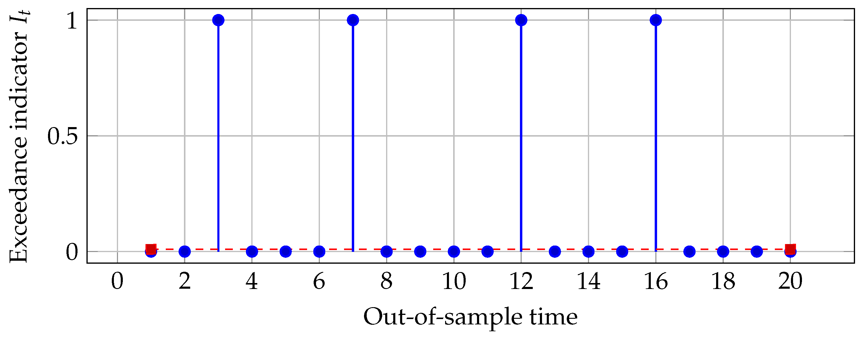
Tail coverage at confidence level (illustrative). Vertical spikes indicate exceedance indicators ; zero values correspond to non-exceedances; the dashed horizontal line marks the nominal exceedance probability ; colors carry no additional categorical meaning. Under correct calibration, exceedances occur with frequency and show no clustering (, ).
5. Empirical Case Study: Climate-Conditioned Sovereign Risk
To assess the empirical reliability and practical implementability of the proposed SCVaR–CES framework, this section presents a real-world application based on publicly available financial and climate data. The analysis investigates sovereign bond repricing in the context of climate transition risk, with particular focus on how spatial heterogeneity in climate hazards and emissions intensity influences the tail distribution of portfolio losses. The study is conducted under the disorderly transition scenario, as defined by the NGFS, which is characterised by delayed policy action followed by abrupt and severe adjustments in carbon pricing, regulation, and market sentiment4. The goal is to evaluate the effectiveness of climate-conditioned tail risk measures, as compared to standard VaR benchmarks in financial risk management and supervisory practices.
Sovereign bond risk is quantified through weekly returns and yield spread changes for (Northern and Southern) European sovereign bond indices, covering the period from January 2015 to December 20245. Figure 6 illustrates the empirical loss and spread dynamics underlying the estimation of the climate-conditioned jump–diffusion model.
Figure 6.
Weekly sovereign portfolio losses and yield spreads (2015–2024). Panel (a) reports weekly portfolio losses constructed from sovereign bond returns. Panel (b) shows the corresponding yield spreads for Northern and Southern European sovereigns.
Climate hazard indicators are obtained from the NGFS climate scenarios, which provide internally consistent transition and physical risk pathways used in macro-financial applications (Battiston et al., 2017; NGFS, 2021). Sector- and region-level emissions intensity data (Scope 1 and Scope 2, measured in e per million euros of revenue) are drawn from CDP disclosures and are used as proxies for transition exposure, in line with the climate finance literature (Bolton & Kacperzyk, 2021; Giglio et al., 2021).
Portfolio exposures are mapped to sector–region buckets using ISO country and sector classifications. Portfolio weights are normalised to sum to one.
Table 4 summarises the data sources, variables, and sample coverage.
Table 4.
Data sources, variables, and sample coverage.
For market-valued instruments, portfolio losses are induced by returns as , where follows the climate-conditioned jump–diffusion process in (1). Accordingly, the empirical loss dynamics satisfy
with the same diffusion and jump components governing tail behaviour.
The time series in Figure 6 exhibit volatility clustering, tail events, and regime shifts consistent with jump–diffusion dynamics. Therefore, these empirical implementations call for adopting a log-linear specification to ensure positivity of jump intensities:
which is a reparameterization of (2). Here, denotes NGFS hazard indices mapped to the region of exposure, and denotes sector–region emissions intensity.
Estimation of parameters proceeds in two stages. First, the diffusion and baseline jump parameters are identified using likelihood-based methods for discretely sampled jump–diffusion processes, following the closed-form approximations of AitSahalia (2002) and the affine jump–diffusion framework of Bates (1996); Duffie et al. (2000). Second, climate sensitivities are estimated via panel regressions linking observed jump occurrences and intensities to hazard and emissions measures, with sector and region fixed effects.
Jump arrival indicators are inferred from discrete-time returns using threshold-based likelihood methods standard in the empirical jump–diffusion literature, ensuring consistent identification of jump times and intensities from observed weekly data. Jump sizes are calibrated from tail exceedances of loss innovations, consistent with the fat-tail structure emphasised in Section 3.3. Parameter stability is assessed using structural break and instability tests (Andrews, 1993; Chow, 1960; Hansen, 2001).
Cross-bucket dependence across regions and sectors is initialised using empirical copulas (Patton, 2006), preserving tail dependence in the joint loss distribution used for the computation of in (3) and in (4).
Table 5 shows the jump-diffusion parameters estimated for sovereign bond portfolios, while Table 6 reports empirical estimates of and across prudential horizons of one, three, five, and ten years, together with classical VaR benchmarks computed on the same loss series. All measures are expressed as positive percentages of portfolio value, with confidence intervals obtained via bootstrap or parametric resampling.
Table 5.
Estimated jump–diffusion parameters for sovereign bond portfolios.
Table 6.
Empirical SCVaR, CES, and benchmark VaR estimates at 99% confidence level (weekly data; percentages of portfolio value).
SCVaR estimates increase monotonically with horizon, from 0.70% at one year to 6.96% at ten years, with relatively tight confidence intervals, while CES values are consistently lower, reflecting the conditional expectation below the quantile, but follow the same upward trajectory. These results confirm that climate-conditioned jump intensities translate into higher downside risk over longer horizons while remaining statistically stable in estimation. Historical and Gaussian VaR track SCVaR closely, with Gaussian VaR slightly above Historical VaR at each horizon, indicating that in the present dataset, hazard sensitivities are modest and the climate conditioning does not dramatically amplify tail risk relative to conventional methods, although SCVaR’s tighter confidence intervals demonstrate its robustness compared to purely statistical benchmarks. EVT estimates tend to be higher and are associated with wider confidence intervals, reflecting the sensitivity of tail extrapolation to limited exceedances. At longer horizons, EVT estimates converge toward SCVaR and Gaussian values, but intervals remain broad, underscoring both the usefulness and fragility of EVT: it highlights potential extreme losses but suffers from instability in small samples. The disorderly scenario amplifies transition risk, producing higher SCVaR values than would be observed under an orderly pathway, and the results demonstrate that SCVaR provides a stable and interpretable measure of climate-conditioned tail risk, with narrower confidence intervals than EVT. EVT, while theoretically appealing, yields wide intervals that may be impractical for supervisory use, and Historical and Gaussian VaR underestimate transition-driven extremes, particularly at shorter horizons. Overall, the findings support the supervisory relevance of SCVaR in stress testing portfolios under abrupt climate policy shifts.
Paying attention to the three-year horizon—the longest horizon over which classical VaR estimators remain empirically meaningful since at longer horizons, non-stationarity and climate-induced structural breaks invalidate standard VaR assumptions—SCVaR exceeds or matches classical VaR benchmarks, with a heavier left-tail risk emerging once conditioning on climate transition hazards is introduced, despite similar point estimates under historical simulation.
The empirical evidence confirms that SCVaR and CES offer three advantages: (i) explicit conditioning on NGFS hazard scenarios ensures consistency with climate stress testing frameworks adopted by central banks; (ii) spatial disaggregation by region and sector enhances interpretability for ICAAP and Pillar 2 capital planning; (iii) bootstrap-validated confidence intervals provide transparency for disclosure and market discipline. These features demonstrate that SCVaR is not only theoretically coherent but also practically applicable in prudential regulation and risk management.
6. Applications
All results in this section rely on the empirically calibrated parameters and loss distributions introduced in Section 5. The figures and tables below therefore illustrate how validated SCVaR outputs can be translated into prudential metrics rather than serving as an additional estimation exercise.
This section illustrates how the spatial stress testing and framework informs prudential decision-making across three domains—bank loan books, pension funds, and sovereign exposures—while keeping reporting aligned with ICAAP, risk appetite, and disclosure dialogue. Results are presented as sectoral point estimates and confidence intervals (Table 7), contrasted across NGFS scenarios in Figure 7, and complemented with diagnostic intervals in Figure 8 and robustness statistics in Table 8. For sovereigns, an illustrative pricing channel is visualised in Figure 9.
Table 7.
estimates across sectors and climate scenarios (illustrative).
Figure 7.
Sectoral across NGFS scenarios (illustrative). Disorderly transitions consistently amplify tail risk.
Figure 8.
Sectoral (disorderly) with bootstrap 95% CIs (illustrative). Bars denote point estimates; whiskers indicate 95% bootstrap CIs; colors carry no additional categorical meaning.
Table 8.
Robustness and sensitivity diagnostics across sectors (illustrative).
Figure 9.
Illustrative association between sovereign spreads and climate vulnerability. Dots represent illustrative sovereign observations; the solid line is a stylised linear fit for exposition; colors are not used to encode additional information.
- Banks (solvency and credit quality). Banks intermediate the largest climate-exposed balance sheets and are particularly sensitive to both transition (carbon-price shocks, policy shifts) and physical risks (e.g., flood- and heat-driven collateral losses). Embedding hazard-linked jump–diffusion dynamics in the credit engine increases tail mass and raises conditional loss quantiles for heterogeneous regional books. In Table 7, the disorderly scenario lifts for banks from 10.2% (baseline) to 15.7% (illustrative), with corresponding increases visible in Figure 7. The bootstrap bands in Figure 8 and the exceedance/structural checks in Table 8 confirm statistical adequacy of these tail estimates. For ICAAP, these outputs translate into (i) climate-adjusted solvency thresholds, (ii) regional concentration limits where spatial hazard indices are elevated, and (iii) overlays where financed emissions proxies materially steepen PD/LGD mappings (as per Section 3).
- Pensions (funding ratio stability). Pension funds face dual channels: asset-side re-pricing (equities, bonds, real estate) and liability-side shifts (longevity and discount rate paths). The spatial reveals that physical risk heterogeneity interacts with transition shocks to amplify tail losses in long-duration portfolios. Illustrative numbers indicate that rises from 7.8% to 11.1% between baseline and disorderly scenarios (Table 7), with cross-scenario contrasts in Figure 7 and precision conveyed by Figure 8. These estimates support IORP II/Solvency II dialogues by (i) quantifying capital-at-risk under scenario/horizon matrices, (ii) identifying region–sector concentrations that drive tail events, and (iii) documenting uncertainty via confidence bands and coverage diagnostics (Table 8).
- Sovereigns (fiscal vulnerability and market pricing). Sovereign balance sheets are exposed through disaster response, infrastructure replacement, tax-base erosion, and market repricing of risk premia. The spatial mapping connects regional hazards to fiscal channels and to sovereign spread dynamics. The sectoral summary in Table 7 shows increasing from 9.5% to 13.4% (baseline to disorderly), while Figure 9 illustrates a positive association between a climate vulnerability index and bond spreads (expository). These outputs guide (i) climate-aware debt sustainability analysis (DSA) with tail metrics, (ii) targeted buffers where hazard exposure clusters geographically, and (iii) scenario-calibrated stress overlays that reflect jump risks rather than smooth narratives alone. Statistical robustness in Table 8 supports supervisory use.
- Supervisory reporting and policy linkage. Together, Table 7 and Figure 7 and Figure 8 form a compact reporting pack: point estimates and 95% CIs by scenario/horizon (capital relevance), sector/region contributions (limit-setting and concentration management), and validation diagnostics (auditability). In ICAAP and Pillar 2 exchanges, institutions can (i) benchmark climate-adjusted capital against / ranges, (ii) set early-warning thresholds where disorderly outcomes approach risk-appetite limits, and (iii) disclose a transparent bridge from alignment metrics (e.g., GAR) to risk-sensitive tail measures. The framework’s spatial granularity supports geographically differentiated overlays consistent with supervisory expectations and emerging disclosure standards.
7. Discussion
This paper has shown that an econometric and simulation-based framework for spatial stress testing and Spatial Climate Value-at-Risk (SCVaR) yields risk measures that are statistically disciplined, spatially explicit, and directly usable for prudential decision-making. Relative to narrative scenario analysis or exposure-only indicators, the proposed approach embeds climate-linked jump–diffusion dynamics and explicit robustness procedures, thereby turning climate stress testing from a descriptive exercise into a testable risk-measurement process.
Importantly, the empirical application in Section 5 demonstrates that the proposed SCVaR framework is not merely a theoretical construct but can be calibrated using publicly available data and standard econometric techniques. The estimation of jump intensities, jump sizes, and climate sensitivities from observed financial time series confirms that climate-related shocks manifest as statistically identifiable tail events. Moreover, the comparison with classical VaR benchmarks highlights that diffusion-only models systematically understate tail risk under climate stress, whereas SCVaR delivers materially higher and more informative risk measures at supervisory confidence levels.
Three empirical patterns stand out. First, climate-augmented jump–diffusion dynamics allocate materially more probability mass to the far right of loss distributions (Figure 10), resulting in higher tail metrics at supervisory confidence levels. The scenario–horizon matrix in Table 9 and the compact panel of point estimates and intervals in Figure 11 make this visible across Orderly, Disorderly, and Hot-house pathways and across near- and medium-term horizons. Second, spatial heterogeneity is economically significant: contributions by sector and region (Figure 12) indicate that concentrated exposures to high-hazard geographies drive disproportionate shares of portfolio SCVaR, a result mirrored in the Applications figures for banking, pensions, and sovereigns (e.g., Figure 13 and the sovereign spread gradient in Figure 9). Third, the validation layer—coverage and independence of exceedances in Figure 14 and the reported bootstrap confidence intervals in Table 9—supports the adequacy of the loss engine at the relevant quantiles. The sensitivity analysis (Figure 15) further clarifies which hazards (e.g., flood frequency, heat stress) most influence the reported tail metrics, informing targeted data improvements and supervisory overlays.
Figure 10.
Estimated loss densities under a conventional diffusion-only baseline versus a climate jump–diffusion specification (illustrative). The jump–diffusion allocates more probability mass in the far right tail, increasing and .
Table 9.
Scenario–horizon / with 95% confidence intervals (illustrative).
Figure 11.
Scenario–horizon and with illustrative 95% CIs. NT = near term (3y); MT = medium term (10y).
Figure 12.
Heatmap of sector/region contributions to portfolio (normalised to 100%; illustrative). Darker cells indicate concentration risk.
Figure 13.
Sectoral across NGFS scenarios with 95% bootstrap confidence intervals (illustrative).
Figure 14.
Exceedances around the theoretical rate (dashed line). Spikes indicate exceedances (); the dashed line marks the nominal exceedance probability; colors are not used to encode information. Absence of clustering supports conditional coverage.
Figure 15.
Tornado chart of sensitivity of to key inputs (illustrative). Bars show the change in when each factor is perturbed by , holding others fixed. Hazard drivers (flood, heat, drought, storm) dominate the right tail, with transition () and financed-emissions proxy effects material but smaller.
These results have immediate consequences for ICAAP, risk appetite, and Pillar 2 dialogue. First, SCVaR and ES provide tail-sensitive thresholds that can be translated into climate-adjusted capital planning: the scenario–horizon grid (Table 9) offers an auditable mapping from climate pathways to solvency needs. Second, the sector/region contribution analysis (Figure 12) enables granular limit-setting and concentration monitoring, consistent with supervisory expectations on governance and risk management. Third, by reporting both VaR and ES with uncertainty bands, the framework aligns with market-risk practice and supports a conservative stance where ES is used as the binding measure for capital overlay. Finally, the Applications results—higher sectoral SCVaR for banks under Disorderly (Figure 13) and a monotone pricing of vulnerability in sovereign spreads (Figure 9)—demonstrate how policy questions (capital buffers, underwriting standards, fiscal risk) can be anchored in model-based and validated quantities.
Despite these advantages, four constraints remain.
Spatial aggregation constitutes an additional limitation. Asset exposures and physical hazards are mapped at the NUTS-2 regional level, reflecting the granularity at which supervisory reporting and harmonised climate datasets are currently available. However, several physical risks—notably floods, wildfires, and heat extremes—are highly localised phenomena. Regional aggregation may therefore introduce spatial smoothing, whereby assets with heterogeneous local exposure profiles are assigned similar hazard intensities.
The direction of the resulting bias is asymmetric. For portfolios concentrated in local hot-spots within a region, NUTS-2 aggregation is likely to underestimate tail risk by averaging extreme local hazards with less exposed areas. Conversely, for well-diversified portfolios within a region, aggregation may slightly overstate risk by assigning elevated hazard levels to assets that are locally protected or geographically distant from the most exposed zones. In both cases, the effect operates primarily through tail compression rather than through changes in central tendencies.
Importantly, this limitation affects the spatial attribution of risk rather than the internal consistency of the SCVaR framework. The methodology is resolution-agnostic and can accommodate finer spatial units (e.g., NUTS-3, grid-level hazard rasters, or asset-level geocoding) as data availability improves, with aggregation performed endogenously at the portfolio level rather than imposed ex ante.
Data gaps persist, most notably for Scope 3 (financed) emissions and granular hazard metrics. The use of proxy ladders is transparent and stress-tested (Figure 15), but filling these gaps would reduce parameter uncertainty and narrow confidence bands.
Long-horizon instability is plausible: parameters linking hazards to jump intensities and volatility may drift across regimes, a risk mitigated here via rolling estimation and sup-Wald checks but still motivating adaptive and time-varying specifications.
Computational burden rises with spatial granularity and joint market–credit simulation; variance reduction and parallelisation alleviate but do not eliminate this cost. These limitations argue for a two-track strategy: near-term deployment of the method with conservative settings and clear uncertainty reporting; and medium-term investment in data curation and adaptive econometric techniques.
An additional limitation concerns the distributional shape of jump magnitudes. While the simulation engine adopts a parsimonious baseline specification for jump sizes, empirical evidence suggests that climate-related losses may exhibit skewness and heavy tails. Sensitivity analysis reported in the Appendix shows that adopting heavier-tailed jump-size distributions leads to higher and CES estimates without altering scenario rankings or sectoral patterns. This reinforces the prudential interpretation of the reported results and motivates future extensions based on EVT or regime-dependent tail modelling.
In addition, future research may explore explicit threshold-based or regime-switching hazard mappings to capture extreme physical risk amplification while preserving the SCVaR framework and its supervisory interpretation.
Figure 16 summarises how the pieces fit. The econometric core (top node) delivers validated tail measures (SCVaR/ES) that feed sectoral applications (left node), which, in turn, motivate policy design (right node)—calibration of climate capital overlays, scenario design for stress tests, and a disclosure bridge where taxonomy-based alignment metrics (e.g., GAR) are complemented by risk-sensitive measures. The dashed feedback loops in Figure 16 reflect practice: new supervisory scenarios or empirical diagnostics trigger re-specification and re-estimation, maintaining the alignment between statistical validity and policy relevance.
Figure 16.
Conceptual triangle linking methodology, applications, and policy. Solid arrows show the main flow from econometric methods to sectoral applications and policy design; dashed arrows indicate feedback loops that trigger re-specification when empirical validation or supervisory updates require recalibration.
The combination of climate-aware jump–diffusion modelling, spatial disaggregation, and a robust validation suite is sufficient to support prudential use today and flexible enough to incorporate better data and methods tomorrow. The empirical patterns across our figures and tables—fatter tails (Figure 10 and Figure 11), material spatial concentration (Figure 12), validated coverage (Figure 14), and clear sectoral ranking (Figure 13)—are consistent and policy-relevant. With these elements in place, climate stress testing can move beyond narrative sensitivity to become an econometrically grounded component of risk appetite, ICAAP, and supervisory capital planning.
8. Policy Implications
The empirical results in Section 5 provide a concrete calibration basis for these policy tools, ensuring that capital overlays and stress-test scenarios are anchored in observed market behaviour rather than purely hypothetical shocks.
Therefore, the results have immediate supervisory relevance along four fronts: capital planning, stress testing design, disclosure alignment, and integration into ongoing prudential processes.
8.1. Climate-Adjusted Capital Buffers
Scenario–horizon SCVaR/ES estimates (Table 9 and Figure 11) provide tail-sensitive thresholds suitable for climate overlays. A pragmatic implementation is a two-step rule: (i) use ES at the supervisory confidence (e.g., ) as the binding measure; (ii) apply a proportional climate add-on where the add-on size is a function of the incremental ES between the baseline and the selected climate pathway (Orderly/Disorderly/Hot-house). Sector/region contribution diagnostics (Figure 12) support targeted overlays for concentrated exposures, consistent with proportionality and risk-based principles.
8.2. Calibration of Supervisory Stress Tests
The market, credit, and hybrid engines translate NGFS pathways into validated loss distributions, allowing supervisors to move beyond deterministic shocks. The coverage and independence checks (Figure 14) and the reported confidence intervals (Table 9) form a transparent validation layer for scenario design. Authorities can (i) set minimum modelling features (climate-linked volatility and jump intensities; spatial mapping to hazards); (ii) require reporting of ES/SCVaR with bootstrap CIs; and (iii) use contribution analysis to define binding “climate concentration” limits within the stress template.
Differentiated GAR and Disclosure Standards
SCVaR/ES complements alignment metrics (e.g., GAR) by quantifying capital-relevant tail risk. A disclosure bridge should reconcile taxonomy-based ratios with risk-sensitive measures: (i) GAR reported at portfolio and bucket level; (ii) SCVaR/ES for the same buckets with 95% CIs; (iii) a short attribution table that decomposes SCVaR by transition vs. physical drivers. This pairing prevents misinterpretation of high alignment as low risk and supports comparability across institutions.
8.3. Integration into ICAAP and Macroprudential Surveillance
Within ICAAP, banks should (i) map scenario–horizon SCVaR/ES to risk appetite thresholds; (ii) embed early-warning indicators tied to hazard elasticities; and (iii) document model risk governance for climate modules (change control, challenger models, and periodic backtesting). At the system level, supervisors can monitor aggregate SCVaR concentration and, where needed, deploy targeted macroprudential tools (sectoral buffers, systemic risk buffers, collateral haircuts, or underwriting standards for high-hazard regions). The sovereign application (Figure 9) further motivates climate-aware fiscal risk surveillance and the consideration of climate contingencies in debt sustainability analyses.
8.4. Implementation Roadmap
A minimum reporting package—scenario–horizon grid (Table 9), sector/region contributions (Figure 12), validation panel (Figure 14)—ensures transparency and auditability. Data gaps (e.g., financed emissions) should be flagged and sensitivity-tested; supervisors may phase in stricter data expectations while permitting documented proxy hierarchies during transition.
Overall, the proposed artefacts align with current supervisory expectations while raising methodological standards through explicit validation and spatial granularity.
9. Conclusions
This paper develops a Spatial Climate Value-at-Risk (SCVaR) framework that links NGFS-consistent transition and physical hazards to portfolio loss distributions through a spatially explicit jump–diffusion engine and a credit-migration block. The methodology integrates validation—bootstrap confidence intervals, exceedance coverage, and structural stability checks—so that scenario results are statistically interpretable rather than illustrative.
A key contribution of the paper is the empirical validation of the proposed framework. Using real financial returns and climate indicators, the analysis shows that the jump–diffusion parameters governing climate risk can be estimated in practice and that their inclusion materially alters tail-risk assessments. This empirical evidence addresses a central limitation of purely scenario-based approaches and supports the use of SCVaR as a quantitative, auditable, and capital-relevant metric for climate stress testing.
Empirically, the framework yields three robust findings. First, tail amplification under disorderly transitions is economically material, with / increases in the upper quantiles relative to diffusion-only baselines (Figure 10; Table 9). Second, spatial heterogeneity is first-order: sector/region contributions reveal concentrated pockets of risk (Figure 12), implying that portfolio steering and collateral policies should be geographically differentiated. Third, model adequacy can be evidenced: coverage statistics and confidence bands (Section 3.7; Figure 14; Table 8) allow supervisors and banks to judge whether estimated climate tails are commensurate with observed exceedances.
Policy relevance follows directly. SCVaR/ES can be mapped to ICAAP capital planning and risk-appetite limits; jump and volatility parameters calibrate climate stress tests; and a disclosure bridge aligns alignment metrics (GAR) with solvency-relevant risk measures. The conceptual triangle in Figure 16 summarises this loop from methodology to applications and policy, with feedback for iterative refinement.
Limitations remain. Data gaps for granular hazards and financed-emissions proxies, long-horizon non-stationarities, and computational cost in high-dimensional spatial simulations warrant caution. Two extensions are most promising. First, machine-learning-assisted hazard mapping and exposure inference can improve spatial resolution and proxy quality while preserving out-of-sample validation. Second, system-wide implementations that embed interbank, pension–sovereign, and collateral networks would extend SCVaR from portfolio to macroprudential analysis, capturing amplification and feedback effects under climate shocks.
To summarise, the paper advances climate-financial econometrics by providing a bank-usable, statistically validated, and policy-ready approach to spatial climate stress testing. It enables supervisors and institutions to move from narrative scenarios and exposure tallies to forward-looking, tail-sensitive measures that can be governed, validated, and integrated into capital and disclosure frameworks.
Funding
This research received no external funding.
Institutional Review Board Statement
Not applicable.
Informed Consent Statement
Not applicable.
Data Availability Statement
The datasets used in this study are publicly available. The original data analysed are derived from open sources (e.g., NGFS, CDP, financial market indices) and are cited in the article. Further inquiries can be directed to the corresponding author.
Acknowledgments
The authors thank the reviewers for their valuable comments and suggestions, which have significantly contributed to improving and elevating the quality of this manuscript.
Conflicts of Interest
The author declares no conflicts of interest.
Abbreviations
The following abbreviations are used in this manuscript:
| ICAAP | Internal Capital Adequacy Assessment Process |
| WACI | Weighted Average Carbon Intensity |
| CRISK | Climate Risk Capital Shortfall |
| SCVaR | Spatial Climate Value-at-Risk |
| PD | Probability of Default |
| LGD | Loss Given Default |
| GAR | Green Asset Ratio |
| ES | Expected Shortfall |
| CES | Conditional Expected Shortfall |
| NGFS | Network for Greening the Financial System |
| CST | Climate Stress Test |
| ECB | European Central Bank |
| BCBS | Basel Committee on Banking Supervision |
Appendix A. Econometric Derivations and Identification
Appendix A.1. Climate-Linked Jump–Diffusion and Notation
Let denote the (continuously compounded) return on instrument i over step . Conditional on information and regional hazards , the return follows
with hazard links
Assume with (downside jumps dominate). Other thin-tailed can be accommodated. Normal jumps allow the closed forms below.
Conditional One-Step Density (One-Jump Approximation)
For small , the probability of ≥2 jumps is . The mixture density of conditional on one period and covariates is
where is the standard Normal pdf. Equation (A3) comes from the convolution of a Normal diffusion shock with a Normal jump size.
Appendix A.2. Log-Likelihood, Score, and Information
Stack parameters as . The log-likelihood for series is
with in (A3). Gradients follow by the chain rule; denote and with the two Normal kernels. Then
Closed forms for are standard for Normal kernels; derivatives of and with respect to climate covariates are transmitted into the score functions. Parameter estimation is performed via maximisation of using the L-BFGS-B algorithm with parameter boxing (, ). Identification requires (i) variation in not collinear with macro controls and (ii) sufficient tail frequency to pin down .
Appendix A.3. GMM and Bayesian Alternatives
Define moments to match conditional variance, excess kurtosis, and hazard-linked slopes, e.g.,
and minimize . For Bayesian inference, set weakly informative priors (e.g., with ; ; ) and sample by HMC or MH. Posterior draws propagate naturally to bands.
Appendix A.4. Asymptotic Properties
Proposition A1
(Consistency and asymptotic normality). Under standard regularity (compact parameter space, identifiability, , and correct specification of (A3)), the MLE and
Sketch of Proof. Uniform LLN and stochastic equicontinuity yield consistency; a quadratic expansion of around plus a central limit theorem for the score implies asymptotic normality. Allowing to be weakly dependent requires HAC adjustments for GMM and robust OPG for MLE.
Appendix B. Validation, Robustness, and Sensitivities
Appendix B.1. Bootstrap Confidence Intervals
For any risk measure , a moving block bootstrap to preserve dependence is implemented. Let b be the block length and B the number of replications. With blocks concatenated to length T, compute the percentile CI
Block length b follows the data-driven rule of (Politis & White, 2004). and the seed are repoted in the replication manifest.
Appendix B.2. Coverage and Independence Backtests
Let . The unconditional coverage test compares with via
The independence test uses a two-state Markov chain with transition counts ; the conditional coverage statistic is (Christoffersen, 1998). The p-values and failure clustering diagnostics are reported.
Appendix B.3. Structural Stability and Breaks
Parameter constancy for are assessed using Andrews (1993) sup-Wald tests over admissible break fractions and Chow tests at pre-specified dates (e.g., major climate events/policy shifts). HAC covariance estimators control for serial correlation in the score.
Appendix B.4. Sensitivity Elasticities
Define standardised elasticities for hazard or transition drivers as
by finite differences are operationally computed holding other drivers at scenario medians and summarise with a tornado chart (Figure 15, main text).
Appendix C. Data, Transformations, and Calibration
Appendix C.1. Inventory and Mapping
Table A1 shows use and mapping to varying the domain.
Table A1.
Data sources and mapping to model covariates.
Appendix C.2. Transformations and Harmonisation
All series are aligned to a monthly (or quarterly) frequency; macro series are interpolated where needed using Denton-Proportional methods; prices are deflated to real terms; are standardised within region to unit variance for sensitivity comparability. Regional concordance uses NUTS-2 ↔ ISO codes with documented crosswalks. Missing Scope 3 is imputed via (H.1)–(H.3) and flagged for sensitivity sweeps.
Appendix C.3. Calibration and Estimation Settings
MLE starts from diffusion-only fits; jump blocks are initialised by excess kurtosis and tail exceedance frequency. Convergence criteria: relative parameter change or gradient norm ; maximum 2000 iterations; OPG standard errors reported alongside bootstrap bands. GMM uses optimal weighting with Newey–West bandwidth selected by plug-in.
Appendix D. Additional Diagnostics and Figures
Appendix D.1. Rolling Stability of Jump Intensity
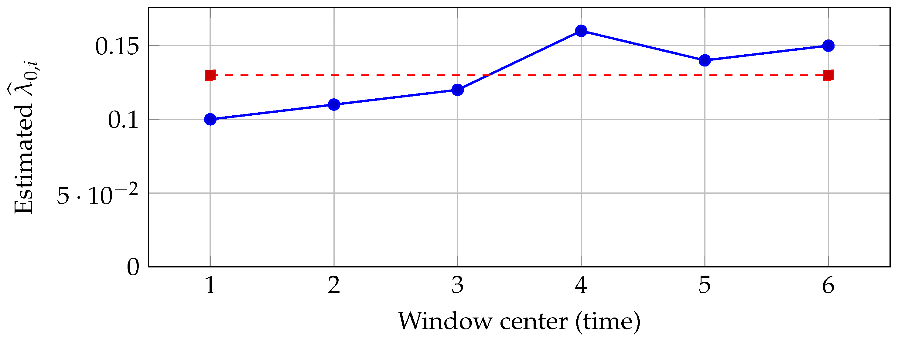
Figure A1.
Rolling estimates of baseline jump intensity with long-run mean (dashed). Confidence bands omitted for brevity; see replication package.
Appendix D.2. Coverage Backtest Series (Illustrative)
Figure A2.
Exceedance indicator vs. nominal rate (dashed). See Appendix B for and test details.
Appendix E. Computation and Reproducibility
Appendix E.1. Data Construction and Layer Integration
This section describes how the theoretical chain Exposure → Hazard → Transition → Financial → SCVaR is operationalised into a unified dataset suitable for Monte Carlo simulation.
- Unit of observation. The fundamental unit of analysis is an asset–region–time triple , where i denotes a financial exposure (e.g., loan, security, or issuer), r a geographical region, and t the time index. All layers are mapped to this common indexing structure, ensuring dimensional consistency across data sources.
- Exposure layer. The exposure layer collects financial positions and balance-sheet weights, including market values, notional amounts, maturities, and sector classifications. Each exposure i is geocoded to region r using issuer domicile, asset location, or collateral geography, yielding a spatially resolved exposure matrix .
- Hazard layer. Physical climate hazards are represented by region-specific indices , sourced from publicly available climate and hazard datasets (e.g., NGFS, reanalysis products). Hazard variables are aligned to the same temporal resolution as financial data and standardised to ensure comparability across regions.
- Transition layer. Transition risk is captured through scenario-dependent macro-financial drivers, such as carbon prices, energy mix shifts, and policy intensity indicators. Let denote the vector of transition variables under scenario s (e.g., NGFS Orderly, Disorderly, Hot-house). These variables are exogenous to individual institutions but heterogeneous across time and scenarios.
- Financial mapping. Hazard and transition variables enter financial outcomes through parameterised link functions that affect returns, volatilities, and jump intensities. Specifically, for each :with analogous specifications for conditional volatility and loss severity. This step transforms climate information into asset-level financial dynamics.
- Final simulation dataset. Combining the exposure, hazard, and transition layers yields a stacked panel dataset , where denotes estimated financial parameters. This dataset constitutes the direct input to the Monte Carlo engine, which simulates joint loss paths across assets, regions, and scenarios. Portfolio losses are then aggregated across to obtain the conditional loss distribution underlying and .
Appendix E.2. Monte Carlo, Variance Reduction, and Seeds
The Monte Carlo procedure operates on the integrated dataset described in Appendix E.1, ensuring that climate hazards and transition pathways enter simulations in a spatially and financially consistent manner. Unless otherwise specified, Monte Carlo paths are simulated per scenario and portfolio with step (monthly) up to years and compute at . Variance-reduction toggles include antithetics (Brownian), a diffusion control variate, and stratified sampling on the upper 5% tail. Master seed and component seeds are fixed and recorded in the run manifest.
Appendix E.3. Jump–Size Distribution
In the Monte Carlo implementation, conditional on a jump arrival, jump magnitudes enter the return and loss dynamics through an additive shock term. For the baseline simulations reported in the main text, jump sizes are drawn from a centred distribution with finite second moments, calibrated to match the empirical scale of observed tail movements. This choice reflects a parsimonious benchmark that facilitates estimation and simulation rather than a literal representation of extreme climate-disaster losses, which are known to exhibit skewness and excess kurtosis.
Appendix E.4. Diagnostics and Distributional Robustness
To assess the sensitivity of tail risk measures to the jump-size specification, diagnostic checks are performed on the estimated jump residuals. Standard normality tests (Jarque–Bera and Shapiro–Wilk) and tail diagnostics indicate departures from Gaussian behaviour in the upper tail, consistent with the empirical literature on disaster losses and climate-related shocks.
Motivated by these findings, the Monte Carlo simulation is repeated under alternative jump-size distributions, including Student-t specifications with finite degrees of freedom and skewed heavy-tailed alternatives calibrated to the same unconditional variance. Across all cases, both and Conditional Expected Shortfall increase relative to the baseline specification, while the qualitative ranking across scenarios, sectors, and regions remains unchanged.
Appendix E.5. Software and Environment
Results are reproducible with either a Python stack (Python 3.11; numpy, scipy, pandas, numba, statsmodels) or Julia stack (v1.10; Distributions.jl, Optim.jl, Random123.jl). Figures use pgfplots (compat = 1.18) and tikz. Hardware: 8–32 cores, 32–128GB RAM; GPU not required.
Appendix E.6. Replication Package
The archive contains /code, /data, and /output with a top-level README. Scripts run_mle.py, run_mc.py, and run_bootstrap.py generate calibrated parameters, loss paths, and diagnostics; make_tables_figs.py exports  -ready CSVs and PGFs. Each run writes a JSON manifest (config hash, git commit, seeds, software versions, checksums) to ensure full provenance.
Appendix F. Extended Results (By Subsector/Region; Illustrative)
Table A2.
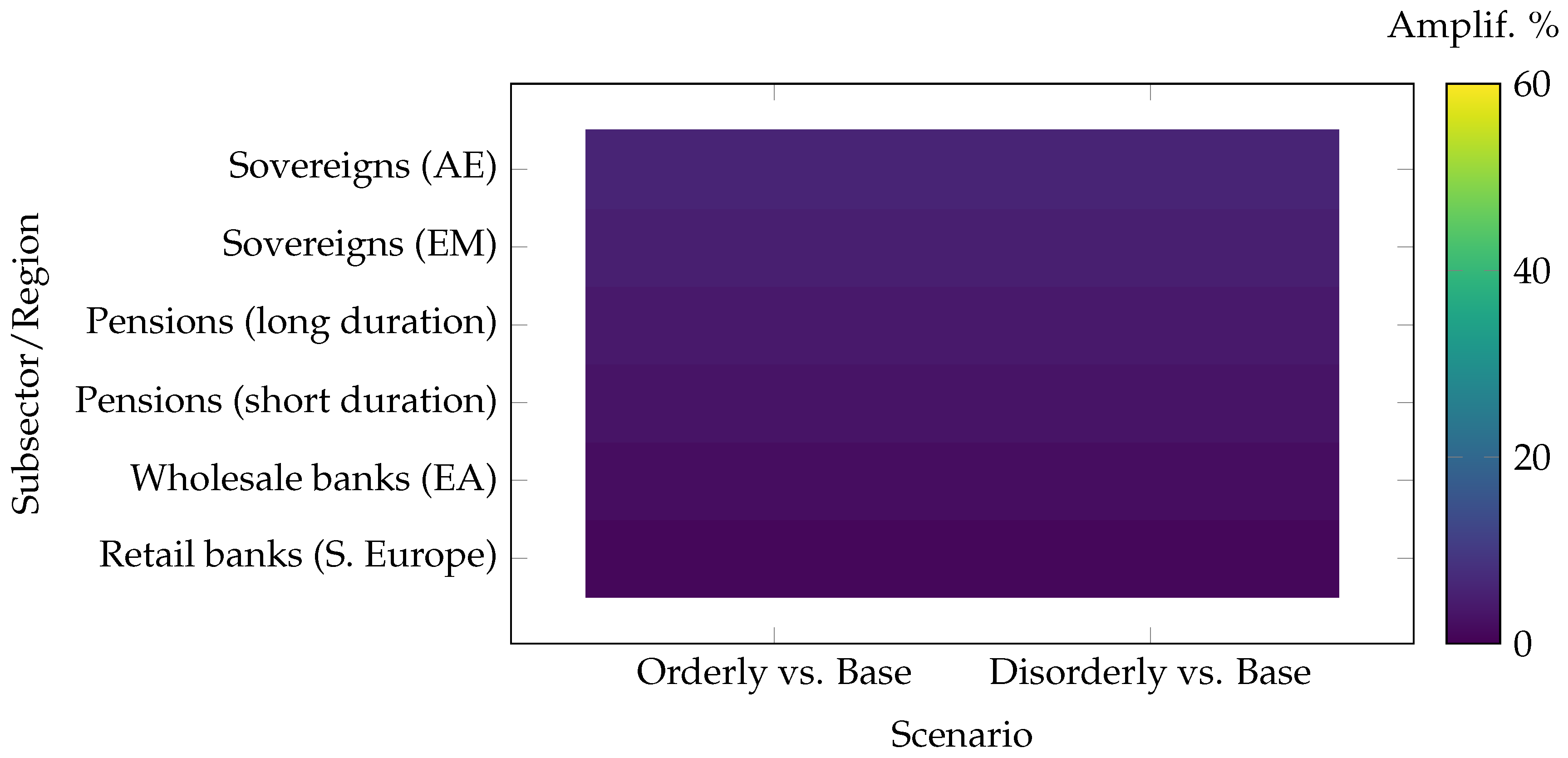
Extended by subsector/region. Losses in % of portfolio value. Amplification vs. Baseline.
Figure A3.
Subsector/region across scenarios (illustrative). Disorderly transitions amplify tails with marked heterogeneity.
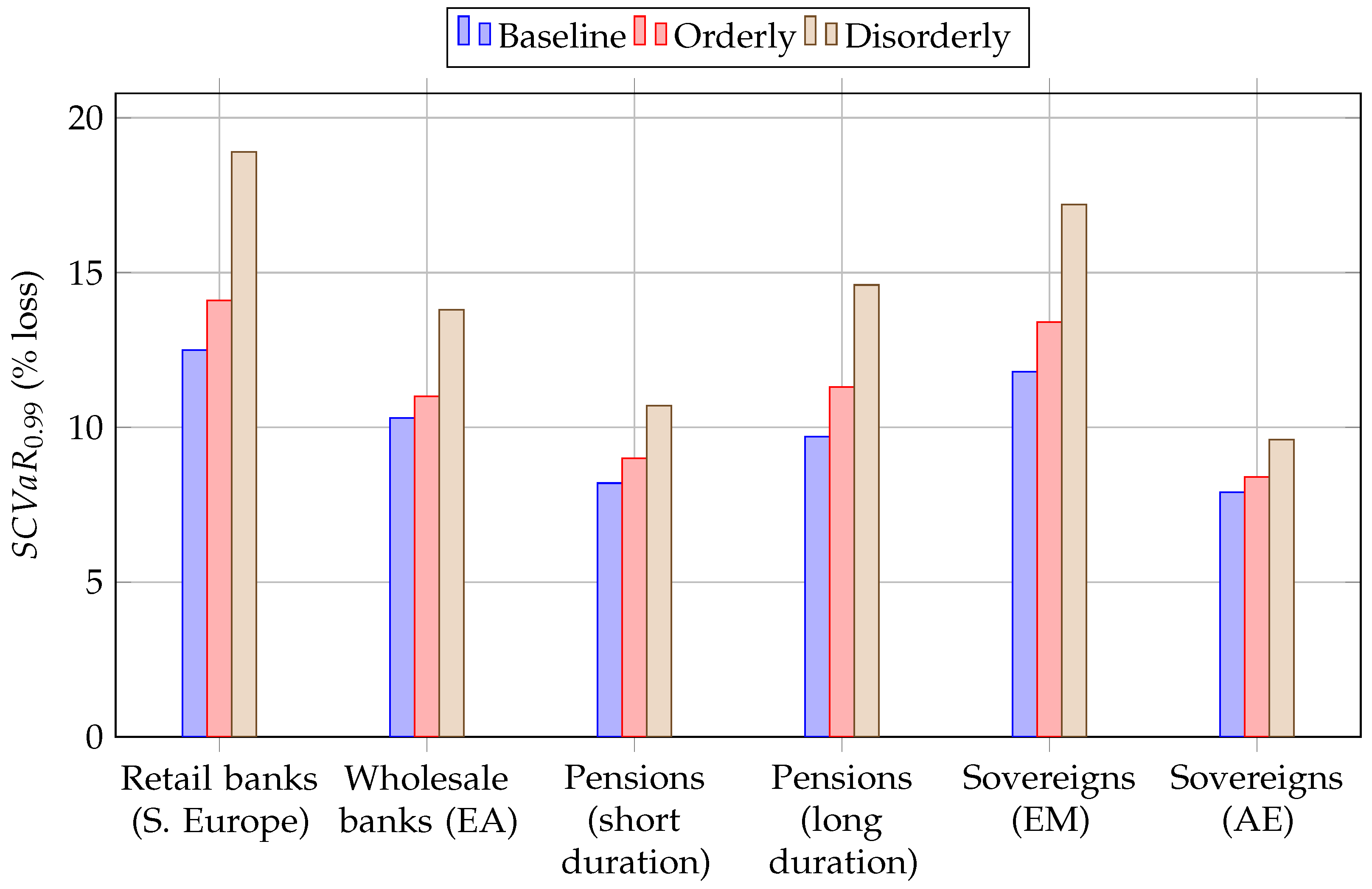
Figure A4.
Amplification of relative to baseline (illustrative).
Notes
| 1 | In the context of financial regulation and climate risk sensitivity analysis, Pillar 2 (also referred to as the Supervisory Review and Evaluation Process, or SREP) is a principles-based framework that requires banks to assess and hold capital against specific risks not fully covered by standardised regulatory minimums, such as governance weaknesses and long-term climate exposures. |
| 2 | When valuation necessitates discount factors beyond the scenario path for policy/term rates, a short-rate model (e.g., Vasicek) calibrated around the scenario mean is employed. Collateral marks for secured credit incorporate spatial climate haircuts (e.g., floodplain exposure), which influence LGD and haircuts used in the credit engine. |
| 3 | The baseline benchmark is a conventional diffusion-only, non-spatial stress set-up akin to regulatory pilots (Acharya et al., 2020; Batten et al., 2020). |
| 4 | This scenario is widely used in supervisory stress testing because it generates stronger transition shocks than the Orderly scenario and highlights vulnerabilities that may remain hidden under smoother pathways. By focusing on the Disorderly case, the study emphasises the tail risks associated with abrupt climate policy shifts, which are of particular concern to regulators and long-term investors. |
| 5 | This sample period encompasses both tranquil and stress episodes and aligns with the horizon adopted in recent climate stress testing exercises conducted by central banks and supervisory authorities (Alogoskoufis et al., 2021; ECB, 2022). |
References
- Acerbi, C., & Tasche, D. (2002). On the coherence of expected shortfall. Journal of Banking & Finance, 26(7), 1487–1503. [Google Scholar] [CrossRef] [Scilit]
- Acharya, V. V., Berner, R., Engle, R., Jung, H., Stroebel, J., Zeng, X., & Zhao, Y. (2023). Climate stress testing. Annual Review of Financial Economics, 15(1), 291–326. [Google Scholar] [CrossRef] [Scilit]
- Aït-Sahalia, Y. (2002). Maximum likelihood estimation of discretely sampled diffusions: A closed-form approximation approach. Econometrica, 70(1), 223–262. [Google Scholar] [CrossRef] [Scilit]
- Alogoskoufis, S., Dunz, N., Emambakhsh, T., Hennig, T., Kaijser, M., Kouratzoglou, C., Muñoz, M. A., Parisi, L., & Salleo, C. (2021). ECB’s economy-wide climate stress test. Available online: https://www.ecb.europa.eu/pub/pdf/scpops/ecb.op281~05a7735b1c.en.pdf (accessed on 1 September 2025).
- Andersen, T. G., & Lund, J. (1997). Estimating continuous-time stochastic volatility models of the short-term interest rate. Journal of Econometrics, 77(2), 343–377. [Google Scholar] [CrossRef] [Scilit]
- Andrews, D. W. (1993). Tests for parameter instability and structural change with unknown change point. Econometrica: Journal of the Econometric Society, 61(4), 821–856. [Google Scholar] [CrossRef] [Scilit]
- Apostolou, A., & Papaioannou, M. G. (2024). Capturing tail risks in climate stress tests of investor portfolios. Journal of Impact & ESG Investing, 5(2), 94–103. [Google Scholar]
- Bank of England. (2021). Climate-scenario analysis and stress testing. Available online: https://www.bankofengland.co.uk/climate-change/climate-scenario-analysis-and-stress-testing (accessed on 1 September 2025).
- Basel Committee on Banking Supervision. (2021). Principles for the effective management and supervision of climaterelated financial risks. Available online: https://www.bis.org/bcbs/publ/d530.pdf (accessed on 1 September 2025).
- Basel Committee on Banking Supervision. (2022). Principles for the effective management and supervision of climate-related financial risks. Available online: https://www.bis.org/bcbs/publ/d532.htm (accessed on 25 August 2025).
- Bates, D. S. (1996). Jumps and stochastic volatility: Exchange rate processes implicit in deutsche mark options. The Review of Financial Studies, 9(1), 69–107. [Google Scholar] [CrossRef] [Scilit]
- Batten, S., Sowerbutts, R., & Tanaka, M. (2020). Climate change: Macroeconomic impact and implications for monetary policy. In Ecological, societal, and technological risks and the financial sector (pp. 13–38). Palgrave Macmillan. [Google Scholar]
- Battiston, S., Mandel, A., Monasterolo, I., Schütze, F., & Visentin, G. (2017). A climate stress-test of the financial system. Nature Climate Change, 7(4), 283–288. [Google Scholar] [CrossRef] [Scilit]
- Battiston, S., Monasterolo, I., Riahi, K., & Van Ruijven, B. J. (2021). Accounting for finance is key for climate mitigation pathways. Science, 372(6545), 918–920. [Google Scholar] [CrossRef] [Scilit] [PubMed]
- Bolton, P., Després, M., Pereira da Silva, L., Samama, F., & Svartzman, R. (2020). Green Swans’: Central banks in the age of climate-related risks. Banque de France Bulletin, 229(8), 1–15. [Google Scholar]
- Bolton, P., & Kacperczyk, M. (2021). Do investors care about carbon risk? Journal of Financial Economics, 142(2), 517–549. [Google Scholar] [CrossRef] [Scilit]
- Campiglio, E., Daumas, L., Monnin, P., & von Jagow, A. (2023). Climate-related risks in financial assets. Journal of Economic Surveys, 37(3), 950–992. [Google Scholar] [CrossRef] [Scilit]
- Cevik, S., & Jalles, J. T. (2022). This changes everything: Climate shocks and sovereign bonds. Energy Economics, 107, 105856. [Google Scholar] [CrossRef] [Scilit]
- Chenet, H., Ryan-Collins, J., & Van Lerven, F. (2021). Finance, climate-change and radical uncertainty: Towards a precautionary approach to financial policy. Ecological Economics, 183, 106957. [Google Scholar] [CrossRef] [Scilit]
- Chow, G. C. (1960). Tests of equality between sets of coefficients in two linear regressions. Econometrica: Journal of the Econometric Society, 28, 591–605. [Google Scholar] [CrossRef] [Scilit]
- Christoffersen, P. F. (1998). Evaluating interval forecasts. International Economic Review, 39, 841–862. [Google Scholar] [CrossRef] [Scilit]
- Dafermos, Y. (2022). Climate change, central banking and financial supervision: Beyond the risk exposure approach. In The future of central banking (pp. 175–194). Edward Elgar Publishing. [Google Scholar]
- Duffie, D., Pan, J., & Singleton, K. (2000). Transform analysis and asset pricing for affine jump-diffusions. Econometrica, 68(6), 1343–1376. [Google Scholar] [CrossRef] [Scilit]
- Efron, B., & Tibshirani, R. J. (1994). An introduction to the bootstrap. Chapman and Hall/CRC. [Google Scholar]
- Embrechts, P., Klüppelberg, C., & Mikosch, T. (2013). Modelling extremal events: For insurance and finance (Volume 33). Springer Science & Business Media. [Google Scholar]
- Engle, R. F., & Manganelli, S. (2004). CAViaR: Conditional autoregressive value at risk by regression quantiles. Journal of Business & Economic Statistics, 22(4), 367–381. [Google Scholar]
- European Banking Authority. (2023). Discussion paper on management and supervision of ESG risks for credit institutions and investment firms (EBA/DP/2020/03). Available online: https://www.eba.europa.eu/activities/single-rulebook/regulatory-activities/sustainable-finance/discussion-paper-role-environmental-risks-prudential-framework (accessed on 10 September 2025).
- European Banking Authority. (2025). Guidelines on the management of ESG risks. Available online: https://www.eba.europa.eu/activities/single-rulebook/regulatory-activities/sustainable-finance/guidelines-management-esg-risks (accessed on 15 September 2025).
- European Central Bank. (2020). Guide on climate-related and environmental risks: Supervisory expectations relating to risk management and disclosure. Available online: https://www.bankingsupervision.europa.eu/ecb/pub/pdf/ssm.202011finalguideonclimate-relatedandenvironmentalrisks~58213f6564.en.pdf (accessed on 1 September 2025).
- European Central Bank. (2022). 2022 Climate risk stress test. Available online: https://www.bankingsupervision.europa.eu/ecb/pub/pdf/ssm.climate_stress_test_report.20220708~2e3cc0999f.en.pdf (accessed on 25 August 2025).
- European Central Bank. (2023). Climate stress test methodology. Available online: https://www.bankingsupervision.europa.eu/ecb/pub/pdf/ssm.climateriskstresstest2021~a4de107198.en.pdf (accessed on 5 September 2025).
- Feng, A., & Chen, Y. (2025). Quantile time–frequency connectedness between green finance and shipping markets: The role of climate transition and physical risks. International Review of Economics & Finance, 104704. [Google Scholar] [CrossRef] [Scilit]
- Giglio, S., Kelly, B., & Stroebel, J. (2021). Climate finance. Annual Review of Financial Economics, 13(1), 15–36. [Google Scholar] [CrossRef] [Scilit]
- Gualandri, E., Bongini, P., Pierigè, M., & Di Janni, M. (2024). Climate Risk Scenario. In Climate risk and financial intermediaries: Regulatory Framework, transmission channels, governance and disclosure (pp. 1–6). Springer Nature Switzerland. [Google Scholar]
- Gupta, R., Marfatia, H. A., & Olson, E. (2020). Effect of uncertainty on US stock returns and volatility: Evidence from over eighty years of high-frequency data. Applied Economics Letters, 27(16), 1305–1311. [Google Scholar]
- Hansen, B. E. (2001). The new econometrics of structural change: Dating breaks in US labor productivity. Journal of Economic Perspectives, 15(4), 117–128. [Google Scholar] [CrossRef] [Scilit]
- Jacquier, E., Polson, N. G., & Rossi, P. E. (2002). Bayesian analysis of stochastic volatility models. Journal of Business & Economic Statistics, 20(1), 69–87. [Google Scholar] [CrossRef] [Scilit]
- Jorion, P. (2007). Value at risk: The new benchmark for managing financial risk. McGraw-Hill. [Google Scholar]
- Jung, H., Engle, R. F., & Berner, R. (2025). CRISK: Measuring the climate risk exposure of the financial system. Journal of Financial Economics, 171, 104076. [Google Scholar] [CrossRef] [Scilit]
- Kolozsi, P. P., Ladanyi, S., & Straubinger, A. (2022). Measuring the climate risk exposure of financial assets: Methodological challenges and central Bank practices. Financial and Economic Review, 21(1), 113–140. [Google Scholar] [CrossRef] [Scilit]
- Network for Greening the Financial System. (2021). NGFS Climate Scenarios for central banks and supervisors. Available online: https://www.ngfs.net/en/ngfs-climate-scenarios-central-banks-and-supervisors (accessed on 5 September 2025).
- Patton, A. J. (2006). Modelling asymmetric exchange rate dependence. International Economic Review, 47(2), 527–556. [Google Scholar] [CrossRef] [Scilit]
- Politis, D. N., & White, H. (2004). Automatic block-length selection for the dependent bootstrap. Econometric Reviews, 23(1), 53–70. [Google Scholar] [CrossRef] [Scilit]
- Rania, F. (2025). Reverse mortgages and pension sustainability: An agent-based and actuarial approach. Risks, 13(8), 147. [Google Scholar] [CrossRef] [Scilit]
- Redondo, H., & Aracil, E. (2024). Climate-related credit risk: Rethinking the credit risk framework. Global Policy, 15, 21–33. [Google Scholar] [CrossRef] [Scilit]
- Rogge, E. (2023). Climate change stress testing for the banking system. European Company and Financial Law Review, 20(4), 717–744. [Google Scholar] [CrossRef] [Scilit]
- Task Force on Climate-Related Financial Disclosures. (2017). Final report: Recommendations of the task force on climate-related financial disclosures. Available online: https://assets.bbhub.io/company/sites/60/2021/10/FINAL-2017-TCFD-Report.pdf (accessed on 20 August 2025).
- Trotta, A., Piluso, F., Strano, E., & Ceraso, D. (2025). The climate-related financial risks measurement methodologies: Advances, challenges, and frontiers. Research in International Business and Finance, 79, 103054. [Google Scholar] [CrossRef] [Scilit]
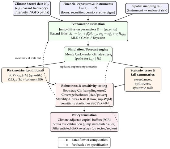
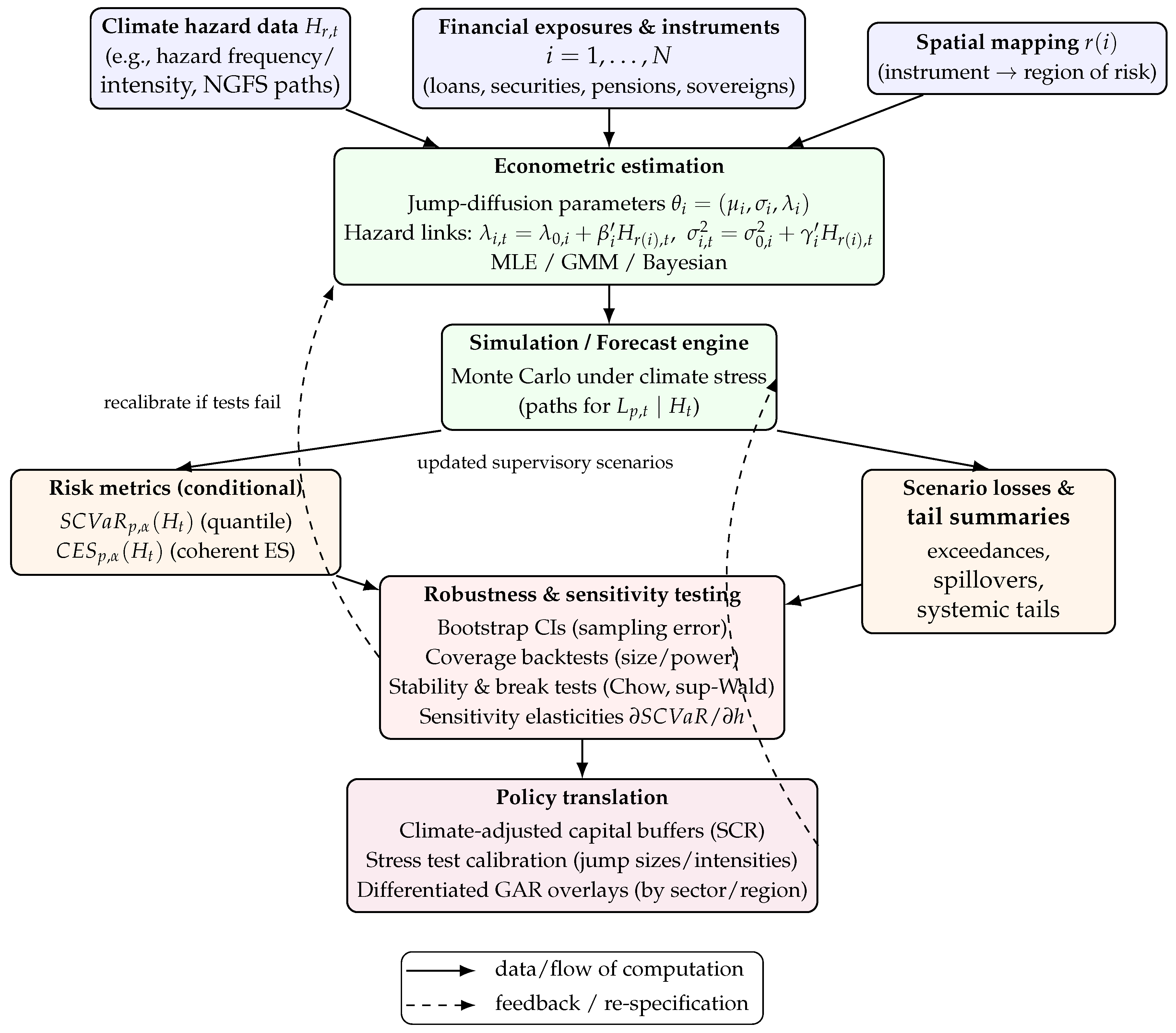
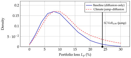
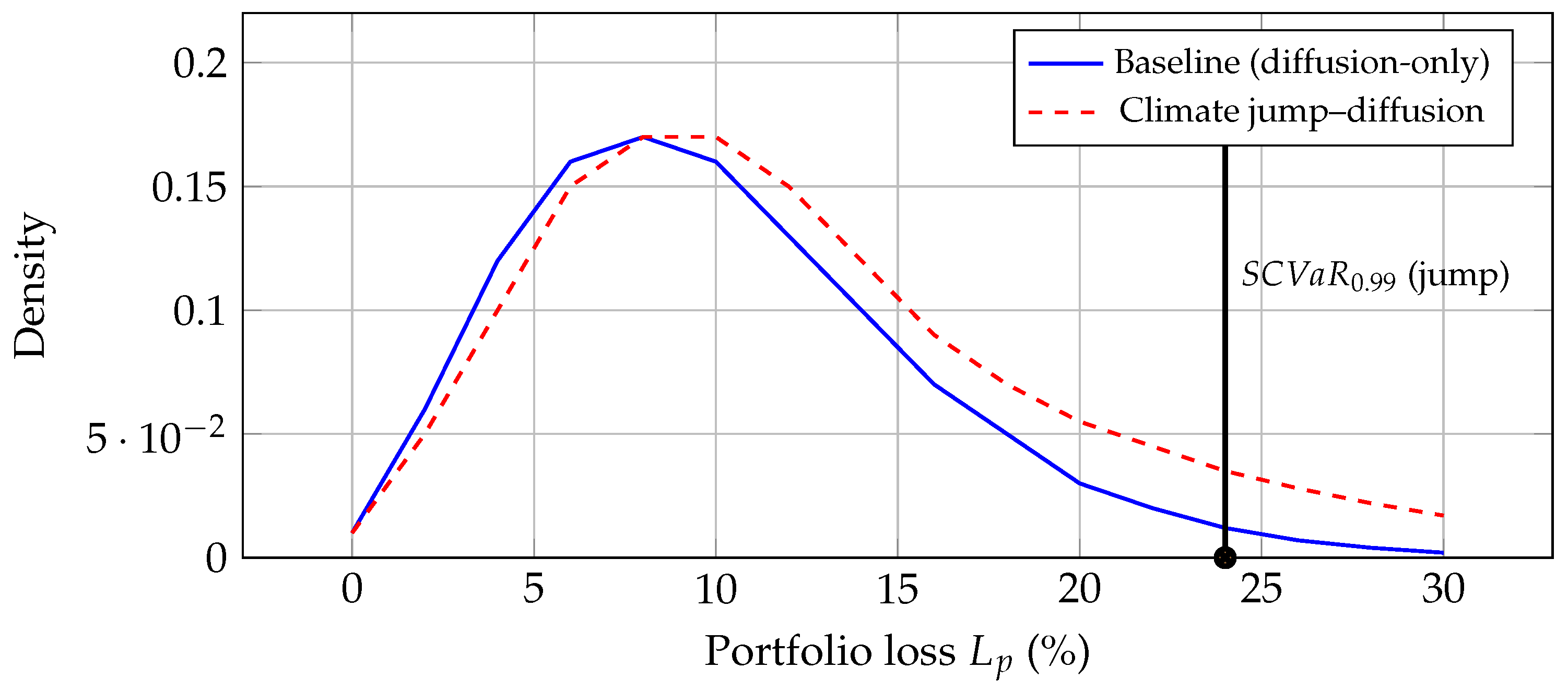
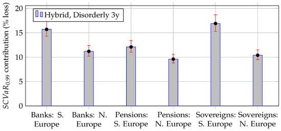
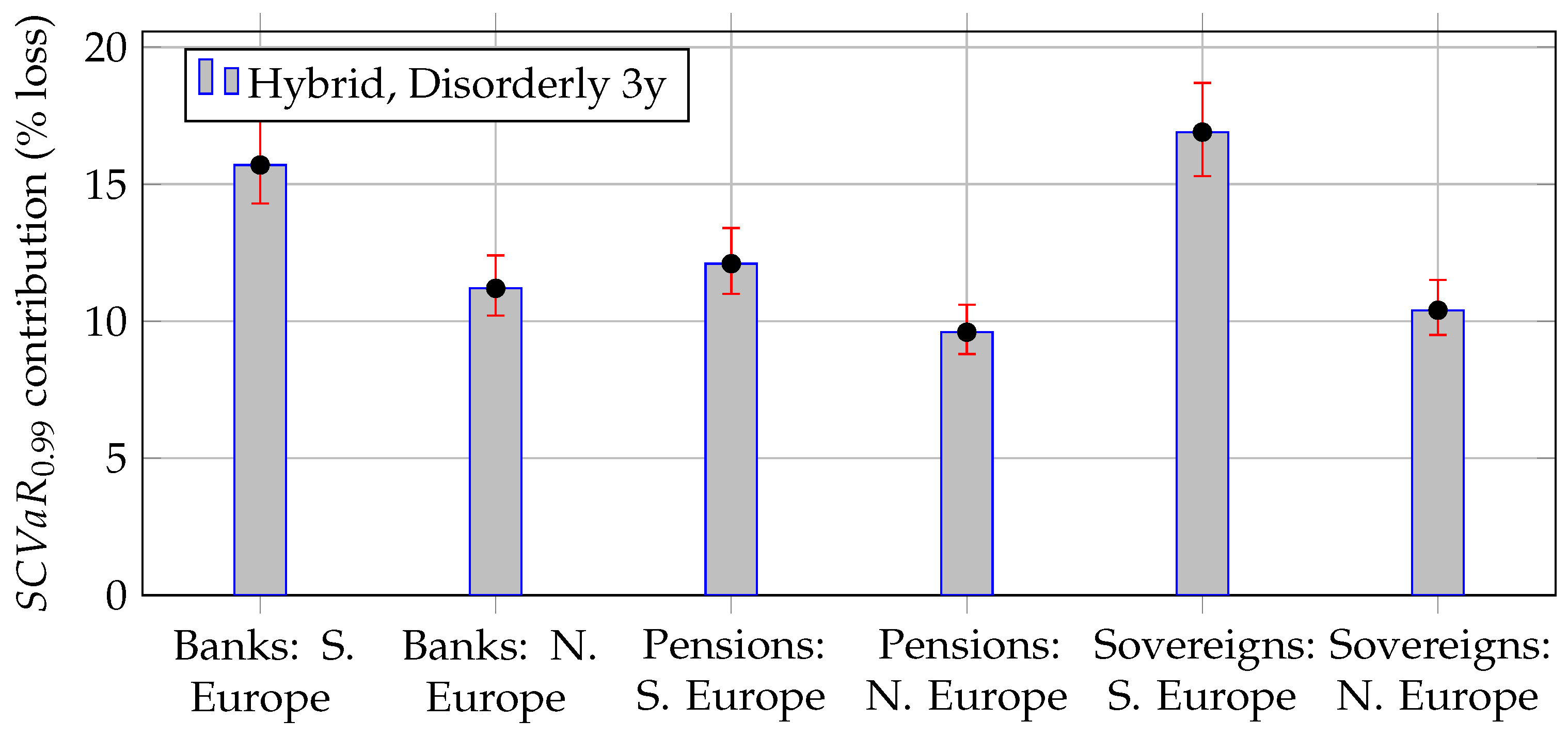
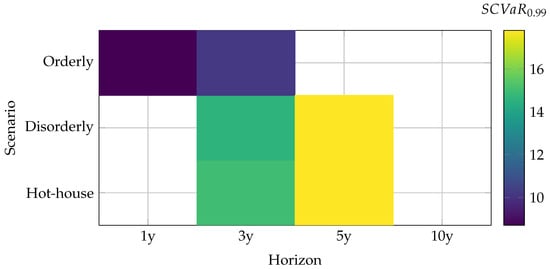
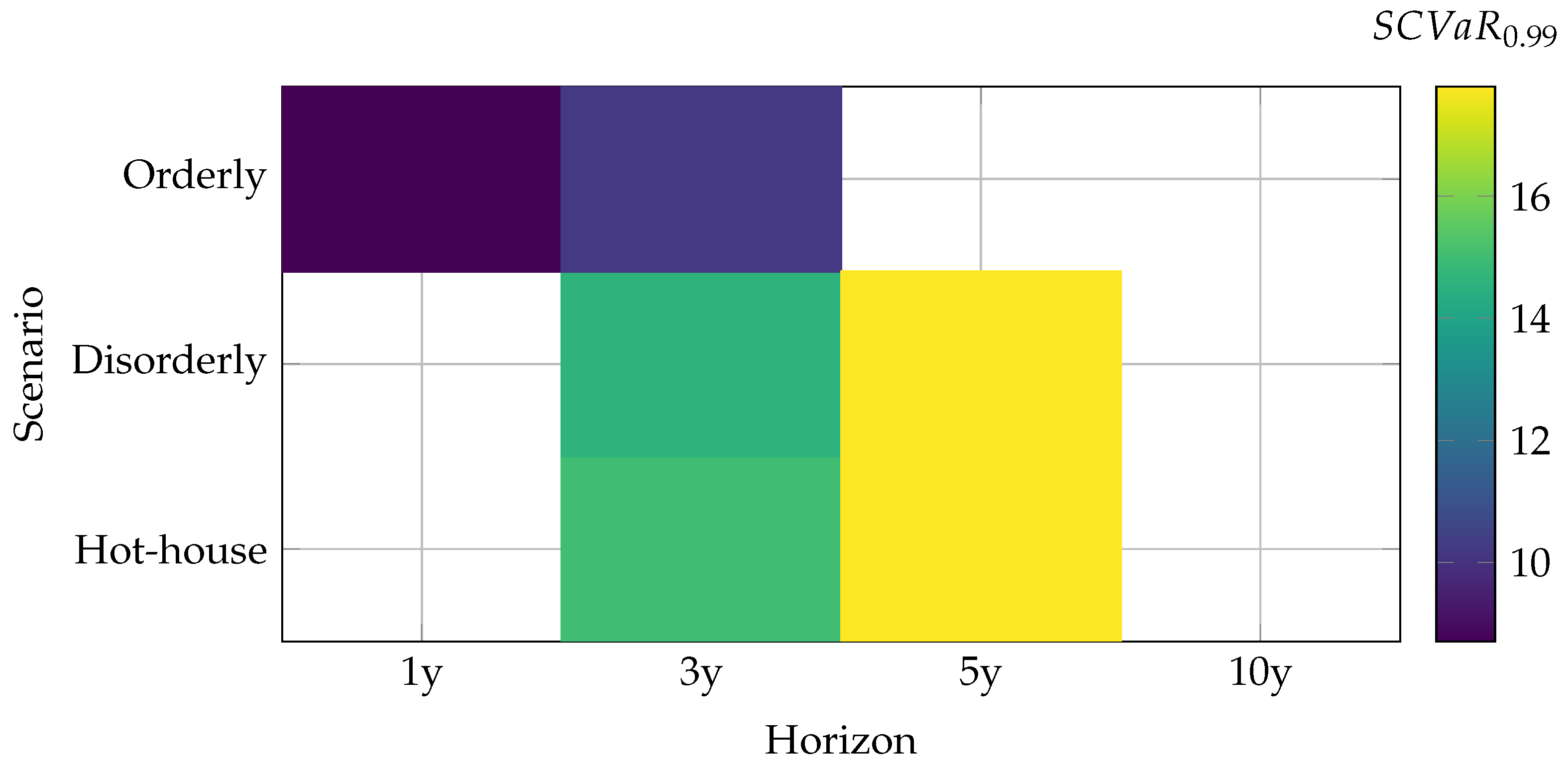
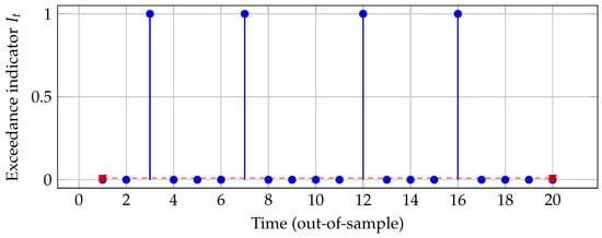
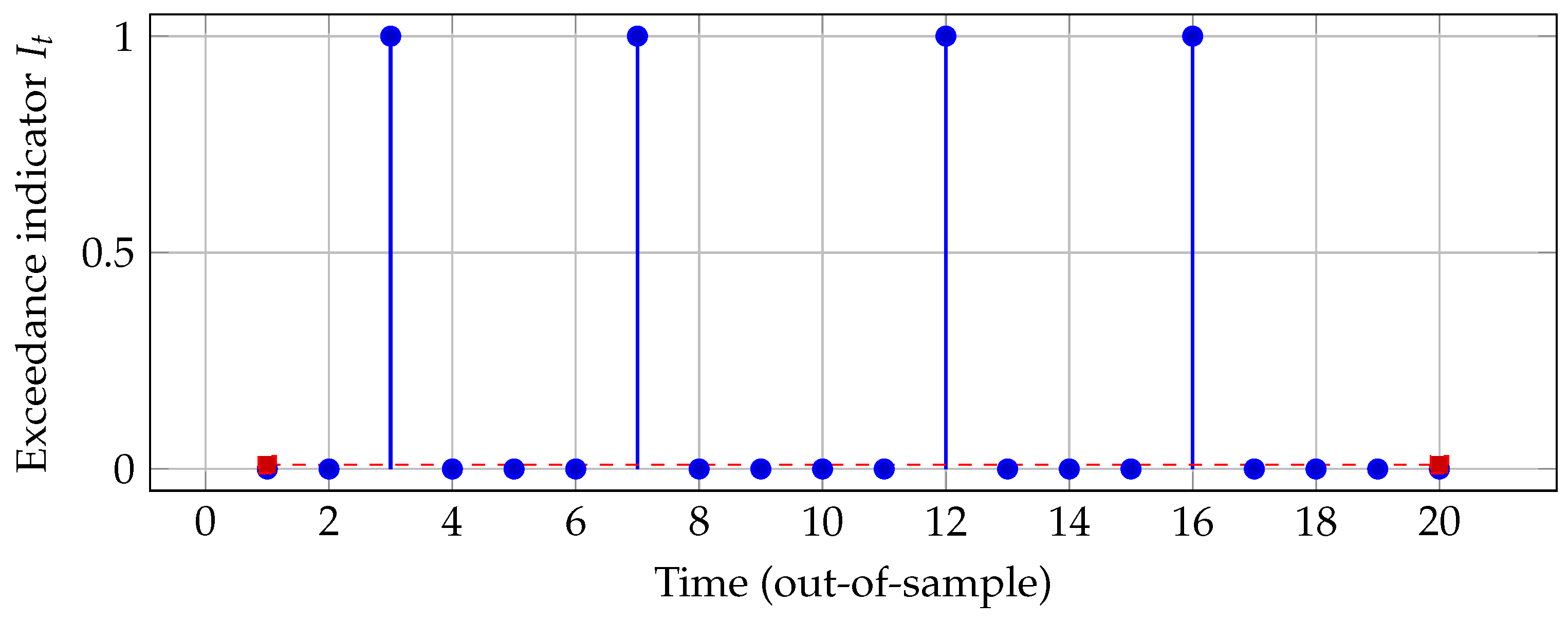
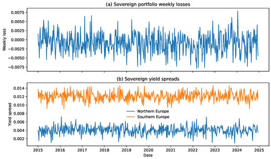
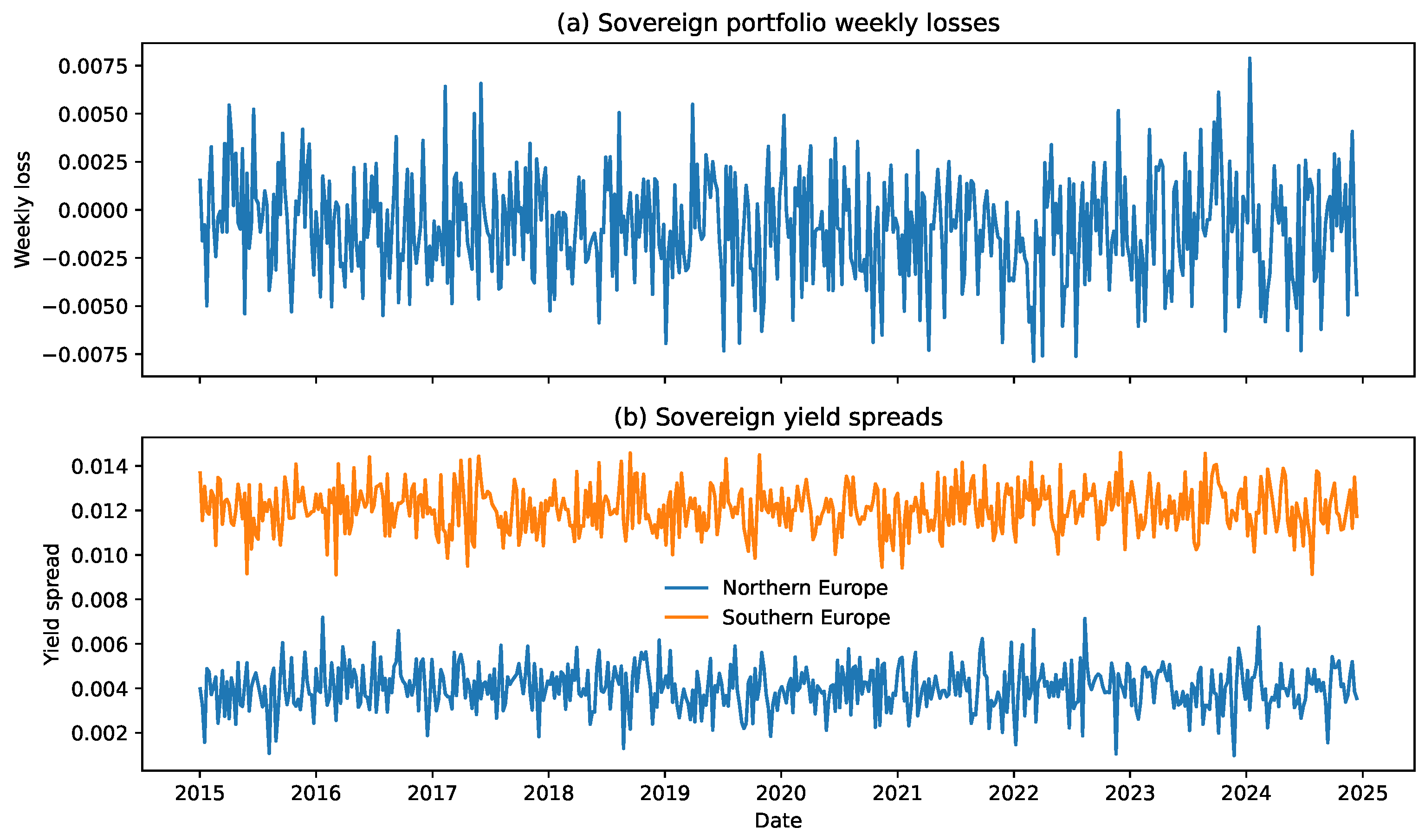
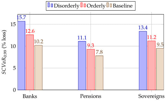
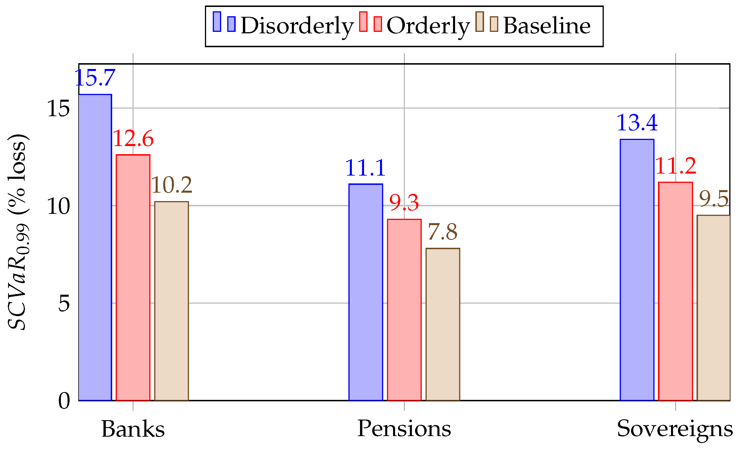
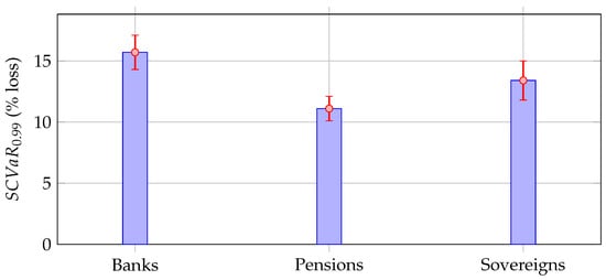
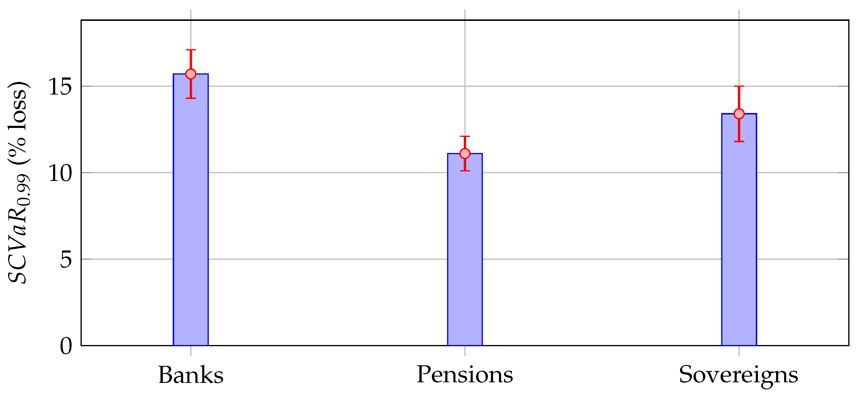
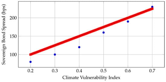
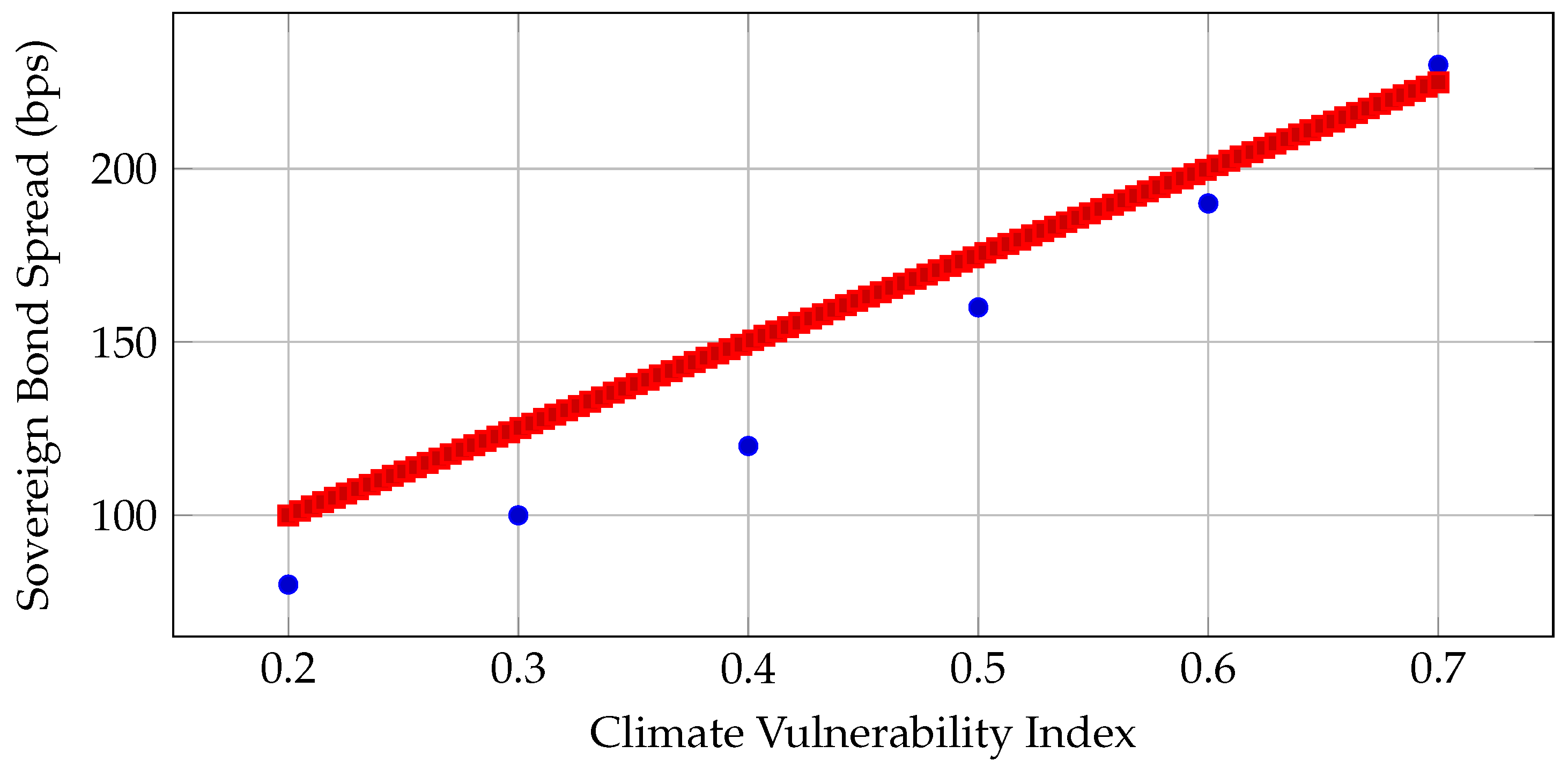
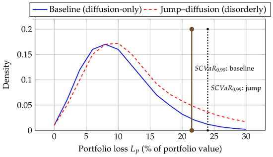
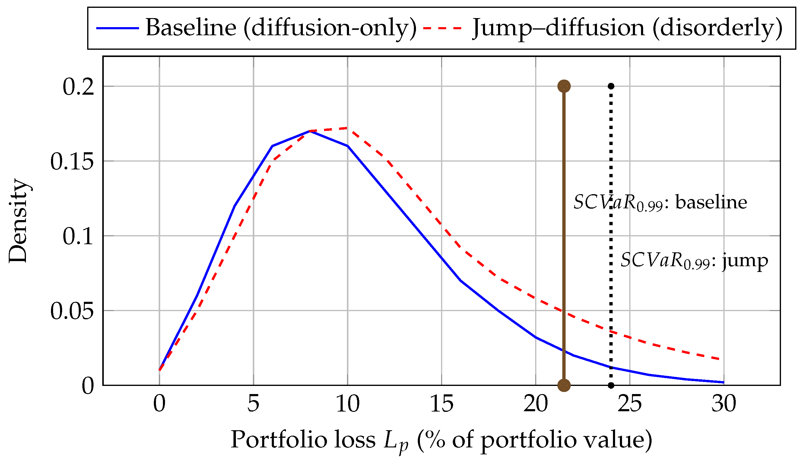
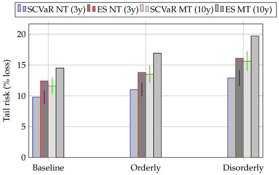
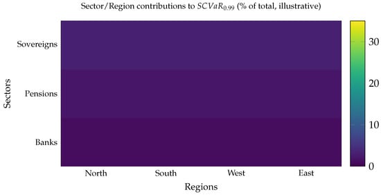
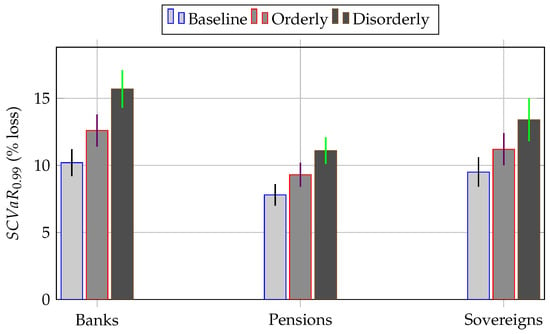
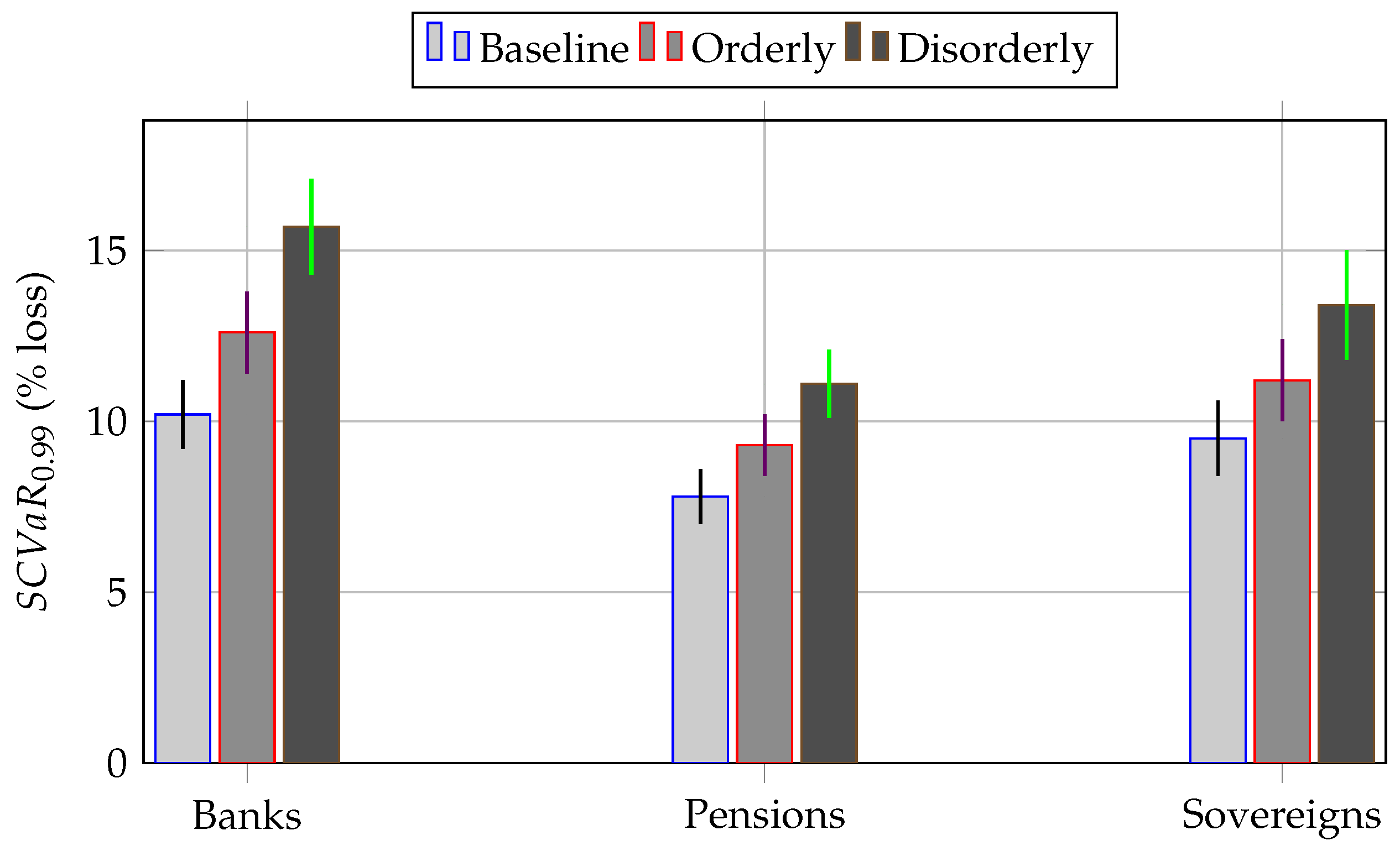
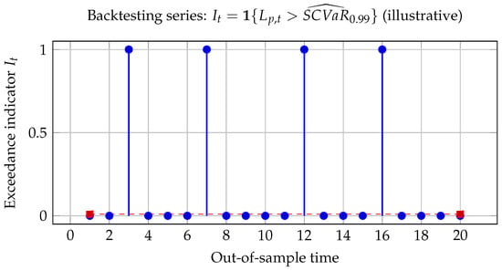
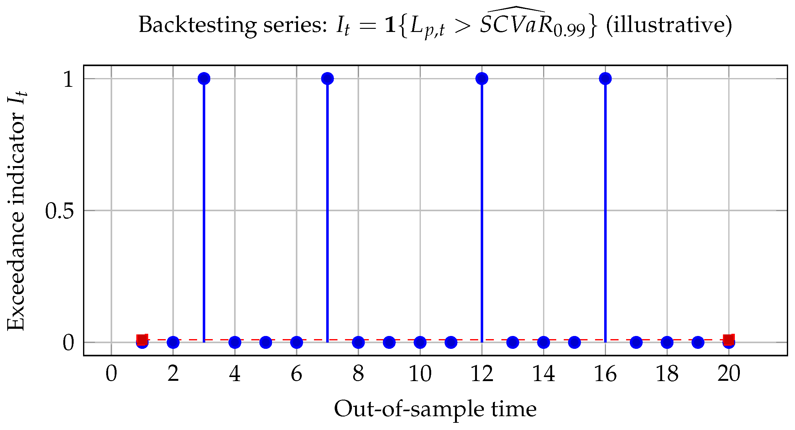
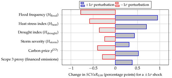
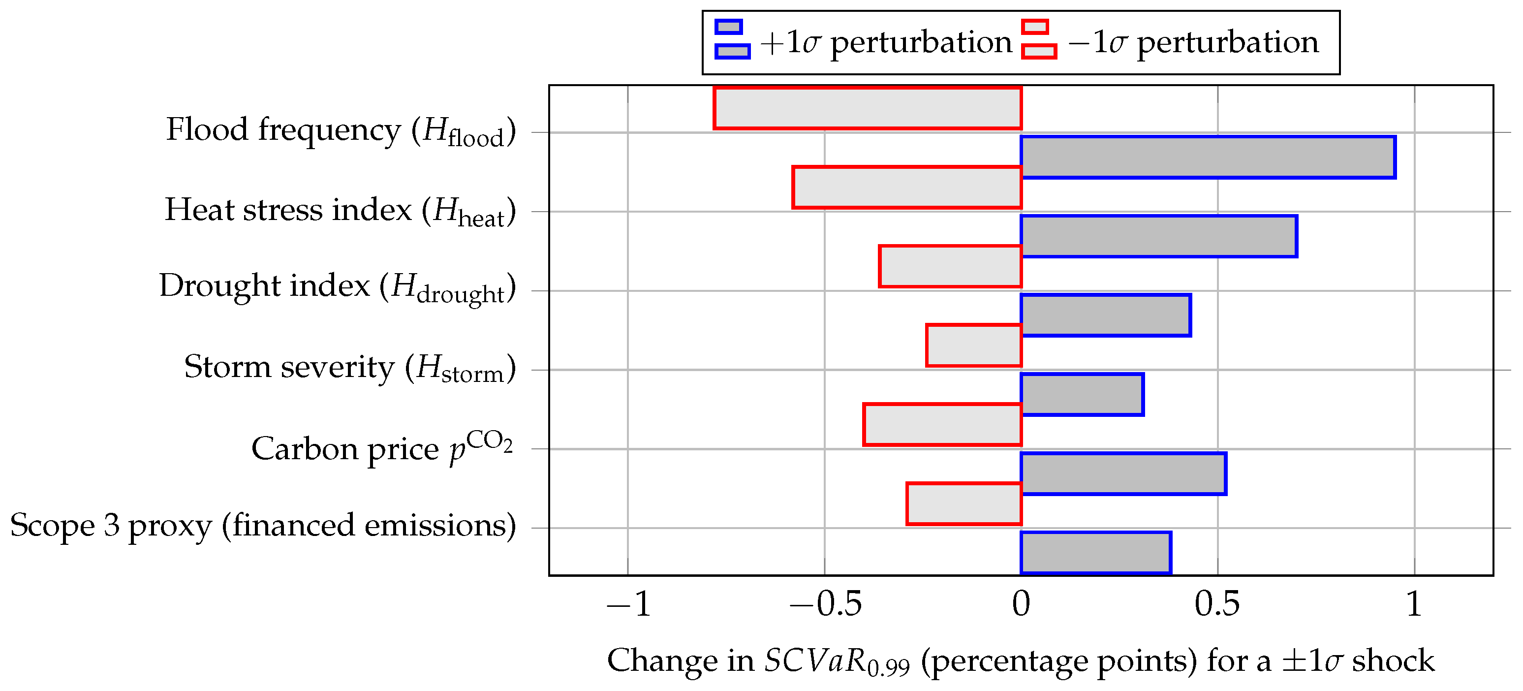
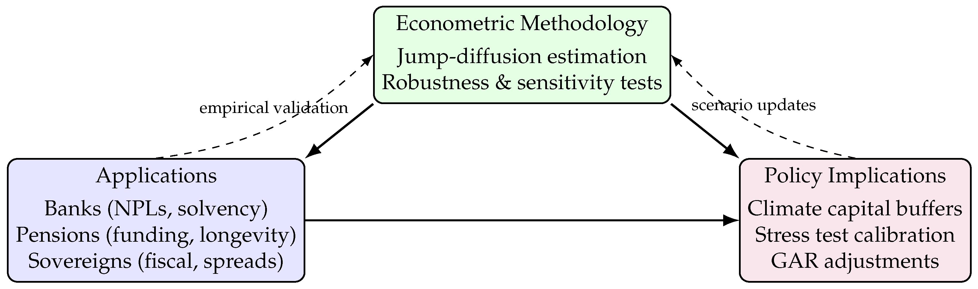

Disclaimer/Publisher’s Note: The statements, opinions and data contained in all publications are solely those of the individual author(s) and contributor(s) and not of MDPI and/or the editor(s). MDPI and/or the editor(s) disclaim responsibility for any injury to people or property resulting from any ideas, methods, instructions or products referred to in the content. |
© 2026 by the author. Licensee MDPI, Basel, Switzerland. This article is an open access article distributed under the terms and conditions of the Creative Commons Attribution (CC BY) license.