


Highlights
What are the main findings?
- The choice of onset estimator alone moved estimated EEG onsets by minutes and changed detection coverage from 45% to 100% in the study data and from 40% to 100% in an independent dataset.
- Conventional 2 SD rules flagged onsets in most no-change trajectories; thresholds calibrated to each trajectory’s design (median 4.7 SD) restore the nominal false-onset rate, and spectrum-preserving surrogates and pseudo-anchors show whether a horizon is specific to the anchor.
What are the implications of the main findings?
- An EEG lead time becomes interpretable when it exceeds an estimator-matched null, is locked to the behavioural anchor and adds information beyond time on task.
- The proposed criteria, calibrated thresholds and checklist allow future studies, including wearable and occupational monitoring, to report early-onset claims in a testable and comparable way.
Abstract
Early-warning claims for electroencephalography (EEG)-based drowsiness detection rest on lead times, yet a lead time depends on how onset is operationally defined and is rarely tested against a null. We developed a benchmarking framework and applied it to seven onset estimators and 32 features from single-channel frontal EEG (17 participants, observer-verified drowsiness reports), with external replication in the DROZY dataset (13 sessions with an eligible vigilance-lapse anchor, of 20 retained). Estimator choice shifted onsets by minutes and changed detection coverage from 45% to 100% (Kendall’s W = 0.53; external W = 0.71; absolute-agreement intraclass correlation 0.05). In simulation, two-standard-deviation baseline rules flagged onsets in 77–88% of no-change trajectories; null-calibrated thresholds (about 4.6 standard deviations) restored a nominal 5% rate. No estimator showed a statistically detectable excess of onsets in the final 150 s before the anchor relative to spectrum-preserving surrogates, a consensus detector fired before pseudo-anchors as often as before the true anchor, and adding EEG to elapsed session time gave no detectable improvement (area-under-the-curve difference 0.01, 95% confidence interval −0.11 to 0.13). Higuchi fractal dimension and line length correlated weakly with measured electrooculography (|r| ≤ 0.15). We propose interpretability criteria, evidence levels and a reporting checklist for early-onset claims.
1. Introduction
Drowsiness is accompanied by changes in alertness, attention, and behavioural control, creating risks in driving and other prolonged vigilance tasks [1,2,3,4,5,6]. Electroencephalography (EEG) provides temporally resolved physiological measurements, but the interpretation of a drowsiness-related signal change depends on both the behavioural reference and the analytic criterion used to identify departure from baseline. In particular, an EEG feature may vary gradually before a self-reported or externally observed event; the time assigned to that change need not coincide with a unique physiological state boundary. This distinction matters when interpreting ‘early detection’ and comparing reported warning horizons.
A substantial literature evaluates EEG drowsiness using alert-versus-drowsy classification, with spectral features, hand-engineered nonlinear descriptors, and machine-learning models [7,8,9,10,11,12,13,14,15,16,17,18]. Reviews of EEG-based driver monitoring and single-channel systems document the diversity of channels, feature sets, labels, datasets, and validation approaches [19]. Prior multimodal studies examined pre-event trajectories [20], while cross-subject single-channel work addresses variation in task duration, signal quality, and individual physiology using learned signal representations rather than explicitly comparing alternative definitions used to estimate transition time [21]. Classification accuracy therefore answers a different question from the time at which a continuously evolving feature first departs from a specified reference.
Transition-sensitive analysis is not new. Earlier EEG/near-infrared spectroscopy (NIRS) work examined changes in frontal beta activity and haemodynamic measures before eye-closure events in simulated driving [20], and an event-oriented EEG index was later developed for detecting drowsiness occurrence [22]. More recent studies describe high-temporal-resolution, single-channel wakefulness probabilities [23] and multimodal forecasting of upcoming drowsiness events [24]. In parallel, nonlinear descriptors including entropy, fractal dimension, and detrended fluctuation measures remain useful summaries of signal organisation, but their behaviour depends on preprocessing, window length, estimator parameters, and non-neural contamination [17,18,25,26,27,28,29,30,31,32,33,34,35,36,37,38,39,40,41,42,43].
What is rarely asked is whether a reported pre-event horizon would also have been obtained in the absence of any event-related change. Onset estimators impose structure of their own: global segmentation methods always return a breakpoint, threshold rules applied to short, autocorrelated baselines can cross a fixed threshold by chance, and slow time-on-task drift can produce monotonic departures that are unrelated to the behavioural anchor. Surrogate-data methods, which test whether a statistic computed on real data exceeds its distribution under a null model preserving selected properties of the signal [44,45], provide a natural way to separate these possibilities, but they are seldom applied to drowsiness-onset estimation. Likewise, feature selection performed on the whole cohort before subject-wise validation can inflate apparent performance [46,47].
The present study therefore asks a narrower and testable question: under which conditions is an early EEG onset interpretable? We first define eight criteria that an onset claim should satisfy (Section 2.1). We then evaluate seven structurally different estimators on single-channel frontal EEG aligned to an observer-verified report of drowsiness, compare every result with simulated no-change trajectories, spectrum-preserving surrogates, pseudo-anchors and anchor jitter, and assess classification against a time-only baseline with fully nested subject-wise feature selection. Finally, we repeat the core analyses on a public multimodal dataset (DROZY) [48] that provides an independent behavioural anchor (psychomotor vigilance lapses) and measured electro-oculography (EOG). Table 1 positions selected studies according to their analytical targets and temporal reference; it is illustrative rather than exhaustive.
Table 1.
Representative EEG-based drowsiness studies in relation to onset definition, temporal alignment, and transition analysis.
The contributions of this work are: (i) a set of eight operational criteria, with associated null benchmarks, for deciding whether an early EEG onset is interpretable; (ii) a demonstration, in simulation, that conventional baseline-threshold rules report pre-anchor onsets on most no-change trajectories, together with null-calibrated thresholds; (iii) a matched comparison of seven estimators showing that horizons and detection coverage are dominated by the operational definition, replicated in an external dataset; (iv) a nested, time-controlled assessment of classification; and (v) an external test, against measured EOG, of the ocular coupling of candidate features. These contributions are methodological; the study does not validate a physiological onset of drowsiness or a deployable warning system.
2. Materials and Methods
2.1. Early-Onset Interpretability Framework
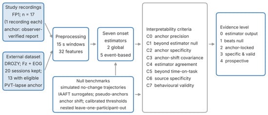
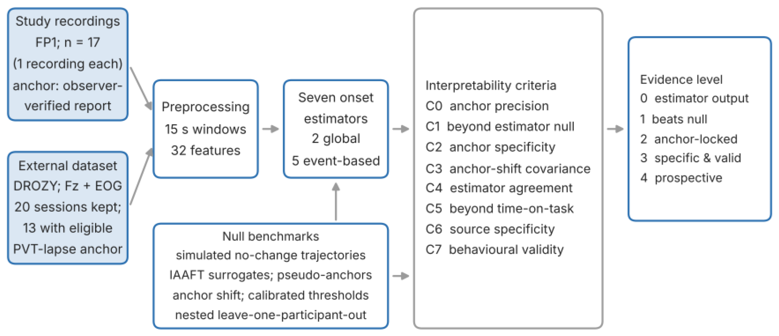
We define an early onset as an estimator-localised departure of a feature trajectory that precedes a behavioural anchor t0. We regard such a departure as interpretable to the extent that it satisfies the criteria in Table 2. C0 is a precondition: the anchor must be timed more precisely than the horizons being claimed. C1–C3 concern whether the departure is a property of the data and of the anchor, rather than of the estimator. C4 concerns the robustness in relation to the operational definition. C5–C7 concern specificity in relation to drowsiness (Figure 1). The criteria are cumulative and define evidence levels: level 0 (estimator output only), level 1 (exceeds an estimator-matched null; C1), level 2 (anchor-locked; C2 and C3), level 3 (specific and behaviourally valid; C5–C7) and level 4 (prospectively validated with causal processing and false-alarm rates on uninterrupted recordings). Its novelty lies in the explicit null benchmarks and decision criteria, not in a new physiological measurement theory.
Table 2.
Criteria for interpreting an early EEG onset and the tests used to evaluate them.
Figure 1.
Analysis framework. Feature trajectories from the study recordings and the external dataset are processed identically, passed to seven onset estimators and evaluated against null benchmarks; the results are graded against criteria C0–C7 to assign an evidence level.
2.2. Participants and Recordings
Twenty-one healthy volunteers aged 21–52 years (12 men and 9 women at enrolment) each took part in one recording session; the 17 participants included in the analysis comprised 10 men and 7 women. All participants provided written informed consent, and the Simon Fraser University Research Ethics Board approved the protocol (certificate 30000343) in accordance with accepted ethical guidelines [49]. Participants reported no known neurological or sleep disorders and were not taking medications known to affect central nervous system function. They were asked to maintain their usual sleep schedule, to obtain at least 7 h of sleep in the preceding 24 h, and to avoid alcohol and caffeine for at least 12 h before testing [50,51].
Three sessions were excluded because more than 40% of their quality-control windows were rejected (43.9%, 94.3% and 98.3%; Section 2.5); in the retained sessions, 4.3–35.4% of windows were rejected. During a code and data audit, the exported file of one further session was found to be a byte-identical copy of another session’s export (same start and end clock times and identical feature values); the original data of that session could not be recovered, and the file was removed. The analysed sample therefore comprised 17 participants with one recording each, and the participant was the inferential unit throughout (Section 2.11).
2.3. EEG Acquisition
EEG was recorded with a BrainLink wireless headset (Macrotellect Ltd., Shenzhen, China) with dry electrodes; the FP1 channel was analysed [52]. The device streams samples at a nominal 512 Hz in 64-sample packets over Bluetooth Low Energy. The exported files carry a wall-clock timestamp with 1 s resolution; per-second sample counts were typically 448, 512 or 576, the mean effective rate per file ranged from 486.6 to 514.1 Hz, and 11–39% of the seconds contained a count outside 502–522. Each file was resampled to a uniform 500 Hz with a single file-level polyphase ratio derived from its mean effective rate. Packet-level jitter within a second could therefore not be corrected, and amplitudes are expressed in device units. A frontal single-channel configuration was chosen for its wearability [1,2,53]; it limits source separation (Section 4.6).
2.4. Protocol and Behavioural Anchor
Sessions were recorded in the evening or at night. In every session, participants sat at a desk and performed a monotonous, low-demand driving simulation on a laptop, and drowsiness was allowed to develop spontaneously [54,55]. The participant’s face and upper body were filmed with a webcam (typically 320 × 240 pixels).
When participants felt that maintaining alertness was becoming difficult, they raised a hand and read the time from the clock of the laptop that was recording the EEG. Two observers, blinded to the EEG, then independently reviewed the videos and, combining the hand raise with head movements, yawning and blinking, agreed on a consensus time of perceived drowsiness, t0. Because t0 was read from the recording computer, it is expressed on the EEG clock; for the eight sessions with available video files, the offset between the video and EEG clocks ranged from −5 to +8 s. Most consensus times fell on whole minutes, so the effective resolution of t0 is approximately one minute. Individual observer timings were not retained, so inter-rater agreement could not be quantified; the influence of anchor uncertainty was instead assessed by jitter (Section 2.8). Furthermore, t0 denotes a reported state, not a verified neural onset.
2.5. Preprocessing
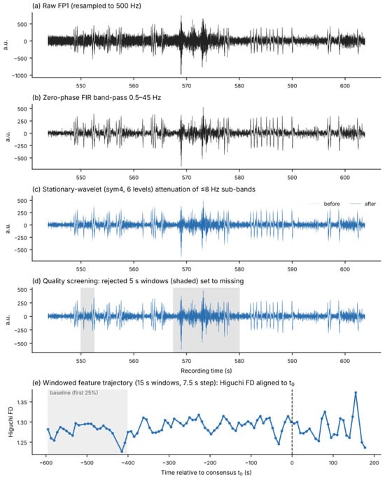
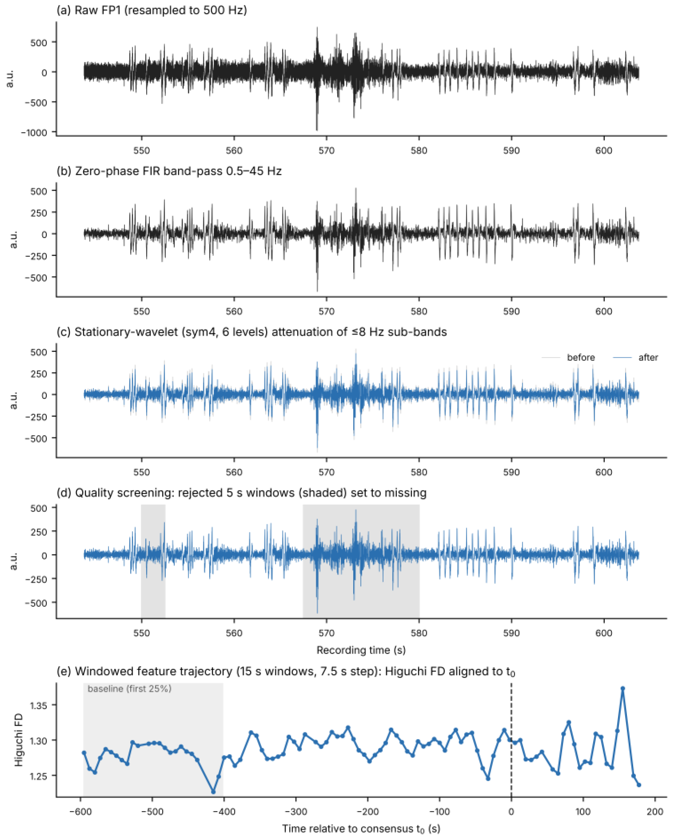
Each resampled signal was filtered with a zero-phase 0.5–45 Hz finite-impulse-response band-pass filter [56,57]. Ocular artefacts were attenuated with a stationary wavelet transform (Symlet-4, six levels) by robust soft-thresholding (k = 1.2 × σ derived from the median absolute deviation (MAD)) of sub-bands centred at or below 8 Hz [58,59]; with this setting, large blink deflections were reduced only partly (Figure 2c). Quality control used 5 s windows with a 50% overlap: a window was rejected if its maximum absolute deviation exceeded 8 robust σ of the recording, if its peak-to-peak amplitude exceeded four times the recording median, or if its standard deviation (SD) was below 5% of the median window SD. Rejected samples were set to missing. For feature extraction, 15 s windows with at least 50% retained samples were kept, and missing samples inside these windows were replaced with zeros before feature computation. Overall, 36.2% of the analysis windows contained some replaced samples (15.3% contained more than 25%); the consequences are examined in Section 3.8 and Section 4.6. Figure 2 shows the processing stages for one recording.
Figure 2.
Processing stages for one recording (S06): (a) raw FP1 signal resampled to 500 Hz; (b) after zero-phase 0.5–45 Hz band-pass filtering; (c) before (grey) and after (blue) stationary-wavelet attenuation of sub-bands ≤ 8 Hz; (d) quality screening, with rejected 5 s windows shaded; (e) resulting windowed trajectory of Higuchi fractal dimension aligned to t0, with the first 25% baseline shaded.
2.6. Feature Extraction
Thirty-two features were computed for each 15 s window advanced by 7.5 s (Table 3 and Table 4): amplitude and statistical descriptors, line length, zero crossings, Hjorth parameters, Petrosian, Katz and Higuchi fractal dimensions (FDs) [28,33,60], sample, fuzzy, permutation and multiscale entropy [26,27,30,34], detrended fluctuation analysis (DFA) [39,40], and Welch band powers, relative powers, ratios and spectral entropy. Sample, fuzzy, multiscale and permutation entropy were computed after resampling the window to 64 Hz; spectral entropy was computed from the full-rate (500 Hz) window. The window time stamp is the window centre, so each window extends 7.5 s before and after its time stamp. The window length was chosen after a preliminary exploration of 5–30 s windows; its influence is reported as a sensitivity analysis (Section 3.5). A low-frequency proxy for ocular activity was defined as the Welch power of the window in the 0.5–4 Hz band; it is numerically identical to the absolute delta-power feature.
Table 3.
Feature-extraction parameters.
Table 4.
Complete set of 32 EEG features by family.
2.7. Feature Trajectories and Onset Estimators
For each recording, windows whose centres fell between 600 s before and 180 s after t0 formed the analysis trajectory (70–104 windows per recording; at least 352 s before t0), giving 1560 windows and 544 recording–feature trajectories. Before estimation, each trajectory was smoothed with a centred three-point moving median. Seven estimators were applied with parameters fixed in advance; the horizon is the time of the estimated onset before t0 (positive values precede t0). Two are global, retrospective segmentation methods that always return a location: (1) piecewise regression, which selects the breakpoint of a continuous two-segment linear fit minimising the residual sum of squares, with at least four points per segment [61]; and (2) changepoint detection, which selects the split maximising a size-weighted standardised mean difference [62,63]. Five are event-based and may return no detection. Four of them (3, 4, 5 and 7) define a baseline from the first 25% of the trajectory, whereas the time-correlation estimator (6) uses no baseline: (3) baseline significance, the first window in which the absolute deviation from the baseline mean exceeds two baseline standard deviations for two consecutive windows; (4) soft-baseline significance, the same rule after additional five-point median smoothing and with a one-standard-deviation threshold; (5) a slope estimator, the first time a five-point running slope departs from the baseline-slope distribution by more than two standard deviations for three consecutive windows; (6) a time-correlation estimator, the split maximising the increase in absolute correlation with time from the pre-split to the post-split segment, retained only if the increase exceeds 0.2; and (7) a two-sided cumulative-sum (CUSUM) estimator on baseline-standardised values with a slack of 0.5 and decision threshold of 4. The baseline, soft-baseline and CUSUM rules search from the first window after the baseline, whereas the slope estimator searches from the first valid running slope, including the baseline period. For persistence-based rules the reported time is that of the first qualifying window, which precedes the time at which persistence could be confirmed.
Features were ranked within each estimator by a score equal to the median horizon multiplied by the detection coverage (recordings with a detection divided by recordings analysed) and by a stability term of 1/(1 + IQR), where IQR is the inter-quartile range of horizons in seconds; scores were normalised to the maximum. Ties retained the fixed feature order, and non-detections entered only through coverage. Redundancy was reduced by a greedy clustering of features with |r| ≥ 0.90 on within-recording z-scored trajectories, seeded in a fixed feature order. Within each cluster, the representative was the member appearing most often among the ten top-ranked features across estimators; remaining ties were broken by a pre-specified interpretability order (spectral ratios and Higuchi FD first, then line length, Hjorth mobility and entropy measures, then band powers and amplitude measures). A feature belonged to the cross-estimator core if it ranked among the ten top representatives in at least four of the seven estimators. These rules are reported for reproducibility; their stability is evaluated in Section 3.5.
2.8. Null Benchmarks
Simulated no-change trajectories (C1). Synthetic trajectories were generated on the same time grid (−600 to +180 s, 7.5 s step) from first-order autoregressive (AR(1)) noise with unit marginal variance. The coefficient φ = 0.41 was the median lag-one autocorrelation of linearly detrended pre-anchor segments of the real trajectories (inter-quartile range 0.26–0.52). Four scenarios were simulated with 200 replicates each: no change; linear drift without onset (1 or 2 SD over the window); a step of 1 or 2 SD at −200 s; and a ramp starting at −300 s reaching 1 or 2 SD at t0. All seven estimators were applied after the same median smoothing. To characterise the baseline-threshold rule further, false-onset probabilities were computed on 4000 no-change trajectories for baseline lengths of 10–100 windows, φ = 0–0.8, thresholds k = 2 or 3 SD, with or without smoothing and a fixed 79-window search period. The null-calibrated threshold k* was defined as the 95th percentile of the largest level exceeded in two consecutive search windows. For application to the real data, k* was simulated separately for each trajectory’s own baseline length, search length and baseline autocorrelation (lag-1 autocorrelation of the detrended baseline, on a 0.05 grid), so that the nominal false-onset rate was 5% for that trajectory’s design.
Spectrum-preserving surrogates (C1, C2). For each real trajectory, iterative amplitude-adjusted Fourier-transform (IAAFT) surrogates were generated, preserving the amplitude distribution and power spectrum, including slow drift, while randomising the temporal placement of changes [44,45]. Surrogates were generated from the sequence of retained windows. Because 15 of 17 recordings contained gaps where windows had been rejected (58 gaps in total), spectral matching is approximate and refers to window order rather than to a uniform time grid. Twenty surrogate sets were analysed with all estimators, and 200 surrogates per trajectory were used for anchor-locked feature change. Anchor-locked change was defined, for each recording and feature, as the mean of windows between 150 s before t0 and t0 minus the mean of the first 195 s, divided by the standard deviation of that early segment. It was expressed relative to the recording’s own surrogate distribution, averaged within participants and tested against zero with the Wilcoxon signed-rank test.
Pseudo-anchors and anchor jitter (C2, C3). For the consensus detector (Section 2.9), pseudo-anchors were placed at every window centre of the full session that left 600 s before and 180 s after it and was at least 180 s from the true t0; the detector was re-run in the same −600/+180 s frame around each pseudo-anchor, and a null distribution of the median lead (one pseudo-anchor per recording per draw, 5000 draws) was formed. For anchor jitter, each recording’s t0 was displaced by a value drawn uniformly from ±30, ±60 or ±120 s (15 draws each); trajectories were rebuilt from the full-session feature files and all estimators were re-applied. Because the stability of the median horizon under symmetric jitter is not by itself sufficient to evaluate C3, we also analysed each trajectory: a common shift d of −120 to +120 s (30 s steps) was applied to t0, the frame was rebuilt and the estimators re-run, and the slope β of the horizon on d was estimated for every recording–feature–estimator combination with at least five detections. β ≈ 1 indicates an onset fixed in session time (determined by the data), and β ≈ 0 an onset that moves with the analysis frame. As a positive control, a step of twice the trajectory SD was added to the same real series at a fixed session time (t0 − 200 s) and the analysis was repeated. Because β ≈ 1 shows only that the estimate stays fixed in session time, the distance between the estimated onset and the true step time was also reported for the positive control. Person-level medians of β are reported with participant-bootstrap 95% confidence intervals (CIs).
2.9. Secondary Analyses
Classification (C5). Windows were taken from the −600/+180 s frame around t0. Windows at least 30 s before t0 were labelled alert and windows at least 30 s after t0 drowsy; windows within 30 s of t0 were excluded (1128 alert and 311 drowsy windows). Logistic regression with balanced class weights and training-fold standardisation was evaluated with leave-one-participant-out cross-validation (17 folds). In nested models, redundancy reduction, estimator-based ranking, the core rule and the ocular-proxy screening were repeated inside each training fold. The inputs included all 32 features, the nested core, the nested ocular-proxy-conservative subset, elapsed time since session start alone, and all features plus elapsed time since session start. t0 was therefore used to define the analysis frame and the labels and, within the training participants, for the estimator-based feature ranking; it was not a model input, and the t0 of the test participant was used only to define its frame and labels for scoring.
Consensus detector. The detector combined Higuchi FD, beta power, permutation entropy and line length. A feature fired at the first window of a two-window run exceeding two baseline standard deviations after centred three-point median smoothing, and consensus was the time at which at least half of the features had fired. We report the retrospectively assigned departure time and the confirmation time, at which the data needed to confirm persistence are available. On a gap-free window grid (7.5 s step), the confirmation time follows the departure time by 22.5 s: 7.5 s for the second window required by the persistence rule, 7.5 s for the following window required by the centred smoother, and 7.5 s from the window centre to its end. Rejected windows can lengthen this delay. Both quantities are also reported for a trailing median smoother, which removes the look-ahead of the smoothing step (minimum delay, 15 s); the zero-phase band-pass filter used in preprocessing remains non-causal, so neither variant is a causal real-time detector. A fixed-time baseline (120–240 s after session start) was also evaluated on full-session data.
Ocular proxy and sensitivity analyses (C6). For each feature and recording, Pearson correlations with the ocular proxy, with time to t0, and with the fraction of retained samples were computed, together with partial correlations with time after adjustment for the proxy. These were Fisher-transformed, averaged within participants and summarised with participant-bootstrap 95% CIs and Benjamini–Hochberg false discovery rate (FDR) correction [64]. Note that, within a recording, time to t0 is a shifted copy of the elapsed session time. Sensitivity analyses repeated the method comparison and core selection after restricting to windows without replaced samples; after excluding windows overlapping the final 15, 30, 60, 90 or 120 s before t0; and after varying the baseline fraction (15%, 35%), threshold (1.5, 2.5 SD) and persistence (1, 3 windows), and with 10 s and 20 s windows (50% overlap). For the latter, the preprocessed signal was rebuilt from the raw recordings with the same pipeline and all features were re-extracted; the rebuilt 15 s features reproduced the original features (largest relative difference 0.2%). The core was also re-derived under correlation thresholds 0.85/0.90/0.95, top-N 5/10/15 and majority 3/7, 4/7 and 5/7, and in 2000 participant-bootstrap samples, in which participants were drawn with replacement and every draw entered the selection as a separate block, so that repeatedly drawn participants carried their bootstrap weight.
2.10. External Dataset
The University of Liège (ULg) Multimodality Drowsiness Database (DROZY) [48] contains 10 min psychomotor vigilance tests (PVTs) [65] performed by 14 young adults on up to three occasions under increasing sleep deprivation, with EEG (Fz, Cz, C3, C4, Pz), vertical and horizontal EOG, electromyography (EMG) and electrocardiography (ECG) sampled at 512 Hz, PVT reaction times and Karolinska Sleepiness Scale (KSS) ratings [66]. Of 36 available sessions, Fz was resampled from 512 to 500 Hz with the same polyphase routine and processed with the same pipeline and parameters as the study data (filtering, wavelet attenuation, quality control, 15 s windows with 7.5 s step and features). Applying the same exclusion rule (more than 40% rejected windows) retained 20 sessions from 11 participants (1489 windows). An independent behavioural anchor was defined as the first PVT lapse (reaction time ≥ 500 ms) followed by another lapse within 60 s and occurring at least 150 s after test start; 15 sessions had such an anchor (152–445 s after test start). The same trajectory rules as for the study data were then applied (−600/+180 s frame around the anchor, at least 10 windows and at least 120 s before the anchor), leaving 13 sessions from 8 participants. Because the tests lasted 10 min, the pre-anchor part of the frame was truncated by the test start (152–415 s available), which bounds the possible horizons. Associations with PVT performance and EOG used all the windows of each session. For each window, vertical EOG was band-passed at 0.3–15 Hz and its 0.5–4 Hz Welch power computed; for correlations, EOG power and the internal proxy were log-transformed (untransformed values are reported as a sensitivity analysis), whereas proxy correlations in the study data used untransformed power, and the mean PVT response speed (1/RT, where RT is the reaction time) was calculated from the stimuli presented within the window. DROZY was used with permission under its licence agreement.
2.11. Statistical Analysis
The participant was the inferential unit. For the method comparison, each participant’s horizons were averaged over features for each estimator (conditional on detection) and compared with the Friedman test; Kendall’s W = χ2/[n(k − 1)] is reported with a participant-bootstrap 95% CI. Because a Friedman test and Kendall’s W quantify systematic, rank-consistent differences between estimators, a low W would not by itself show agreement. Absolute agreement (criterion C4) was therefore assessed on trajectories detected by all estimators by the median pairwise absolute horizon difference, the proportion of pairs within ±60 s, and the two-way random-effects intraclass correlation coefficient (ICC) for absolute agreement, ICC(2,1), each with a participant-bootstrap 95% CI. Detection coverage and conditional horizons were analysed separately (two-part analysis); non-detections were never assigned horizons. Associations between non-detection and trajectory descriptors (number of windows, fraction of replaced samples, a trend-to-residual variance ratio used as an approximate signal-to-noise index, standardised departure from baseline, standardised linear change and non-linearity) were estimated by logistic regression with standard errors clustered by participant. Classification metrics were computed from pooled out-of-fold predictions, with 95% CIs from 2000 participant-bootstrap resamples; differences in the area under the receiver operating characteristic curve (AUC) were assessed with paired participant bootstrap. Multiple comparisons were controlled with FDR. Surrogate p-values were computed as (b + 1)/(B + 1). The reanalysis used Python 3.13 with NumPy 2.5, SciPy 1.18, pandas 3.0, scikit-learn 1.9, statsmodels 0.15, AntroPy 0.2.3, PyWavelets 1.8, pyEDFlib 0.1 and matplotlib 3.11; the random seeds are recorded in the analysis code.
3. Results
3.1. Sample, Data Audit and Anchor Precision (C0)
Before the duplicate export was removed, the audit reproduced the outputs of the original analysis pipeline (for example, 259 of 576 trajectories detected by the slope estimator, 232 complete cases and a cross-estimator core of eight features). All results below use the corrected sample of 17 participants. With an effective anchor resolution of about one minute and video–EEG clock offsets of −5 to +8 s, anchor uncertainty was smaller than the horizons of several minutes under study, so C0 was met in part. Its influence on the results is quantified in Section 3.4.
3.2. Dependence of Coverage and Horizon on the Estimator (C4)
Detection coverage and conditional horizons differed markedly between estimators (Table 5). The method effect was large (Friedman χ2 = 53.7, p = 8.7 × 10⁻¹⁰, Kendall’s W = 0.53, 95% CI 0.44–0.70). The two global estimators did not differ from each other (Wilcoxon p = 0.78), whereas the five event-based estimators differed in both coverage (χ2 = 57.7, p = 9 × 10⁻¹²) and conditional horizon (χ2 = 52.7, p = 9.8 × 10⁻¹¹, W = 0.78). The effect persisted in the 216 trajectories detected by all seven estimators (χ2 = 55.4, p = 3.9 × 10⁻¹⁰, W = 0.54). The time-correlation estimator localised most departures after t0. These tests show that timing depends systematically on the estimator; absolute agreement on the same trajectory was poor. Across the seven estimators, the median pairwise difference was 158 s (95% CI 135–173), only 28% of pairs lay within ±60 s, and ICC(2,1) was 0.05 (0.01–0.09). For the five event-based estimators the values were 128 s, 35% and 0.09, and even for the four baseline-defined estimators they were 60 s, 52% and 0.30 (0.16–0.42), so the differences are of the same order as the anchor resolution or larger (Table S10).
Table 5.
Two-part summary of the seven estimators (17 participants, 544 trajectories). 95% CIs from participant bootstrap.
Non-detection was associated mainly with the size of the departure. Per standard deviation of standardised departure from baseline, the odds of detection increased by a factor of 2.1 (slope), 4.5 (baseline) and 18.0 (soft-baseline, all p < 0.001). The trend-to-residual variance ratio, which also increases with the size of a systematic change, was associated with detection by the baseline (odds ratio (OR) 2.8, p = 0.03) and soft-baseline rules (OR 10.5, p = 0.004) but not by the slope estimator (OR 1.4, p = 0.09). The data-quality indicators, the number of windows and the fraction of replaced samples, were not associated with detection (for the slope estimator, odds ratios 0.87 and 1.34; p = 0.46 and 0.12). Trajectories excluded from the complete-case set similarly showed smaller standardised departures (odds ratio for inclusion 2.3 per SD, p < 0.001). Non-detection by the slope estimator ranged from 19% to 84% across recordings and was highest for theta power (82%). The full recording–feature table is provided as Table S1.
3.3. Estimator Behaviour Without Change (C1)
On no-change trajectories with the autocorrelation of the real data, event-based estimators frequently reported pre-anchor onsets (Table 6). The baseline rule returned an onset in 86% of replicates, the soft-baseline rule in 100% and CUSUM in 98%, at median times of 308, 390 and 338 s before t0, close to their horizons on real data (Table 5). The soft-baseline rule fired, on average, shortly after the end of the baseline segment (−405 s). The global estimators always returned a breakpoint, widely dispersed across the window. When a true change was present, the changepoint estimator located a 2 SD step within 5 s, and CUSUM located a ramp onset with a median error of 4 s (1 SD). The soft-baseline rule fired about 180 s before a step and 80–90 s before a ramp, that is, before the change existed. Full scenario results are given in Table S2.
Table 6.
Estimator behaviour on simulated no-change trajectories (AR(1), φ = 0.41; 200 replicates) compared with real data.
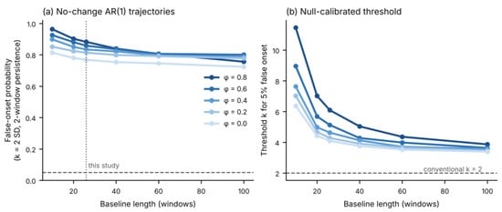
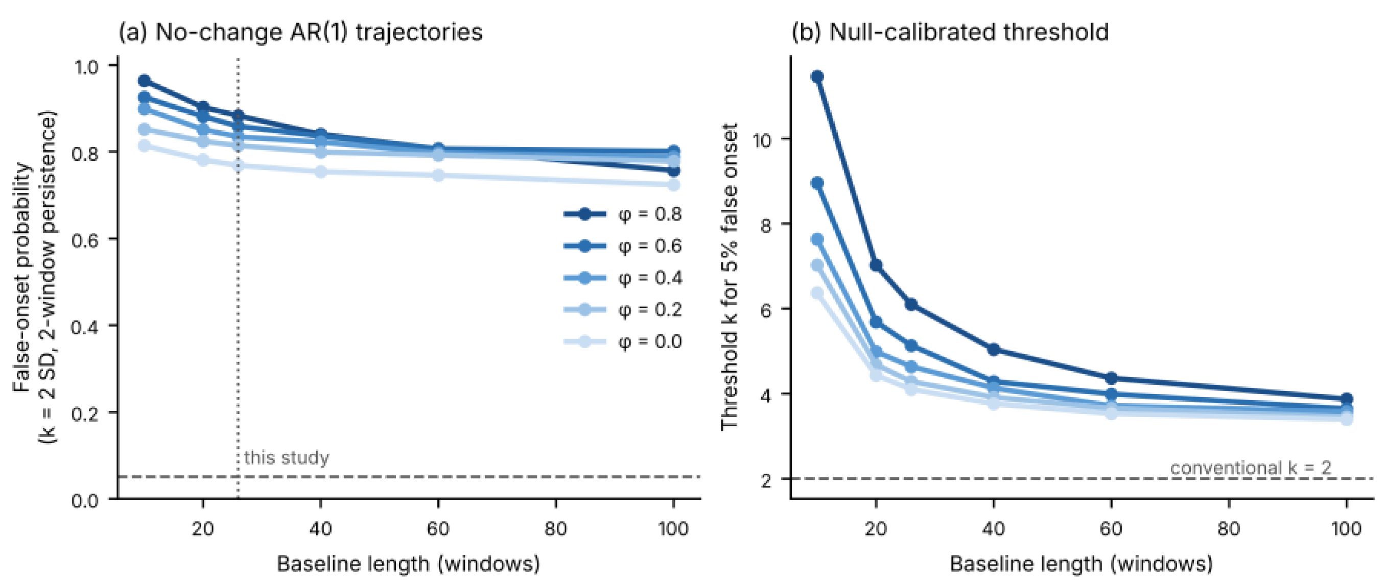
For the conventional baseline rule (k = 2 SD, two-window persistence, smoothing), the false-onset probability was 0.77–0.88 for a 26-window baseline as φ increased from 0 to 0.8, and remained 0.72–0.80 even with 100 baseline windows (Figure 3a). Thus, the multiplicity of search windows, rather than baseline length alone, drives false onsets. For a 26-window baseline and 79 search windows, the threshold needed to restrict false onsets to 5% was 4.1–6.1 SD (4.6 SD at φ = 0.4; Figure 3b). Because the real trajectories differ in length, thresholds were then calibrated for each trajectory’s own design (baseline 17–26 windows, search 53–78 windows; median k* = 4.7, range 4.1–7.9); on fresh AR(1) simulations with these designs the false-onset rate was 6%. Applied to the real data, this rule reduced coverage from 76% to 25%. Under the same rule, however, IAAFT surrogates gave 28.5% coverage (95% range 25.6–31.4%), and there was no statistically detectable excess of detections in the final 150 s before t0 (8.3% vs. 7.4%, p = 0.31). Calibration against autocorrelated noise therefore removes most false onsets, but the remaining detections were not more frequent than on spectrum-preserving surrogates.
Figure 3.
(a) False-onset probability of the baseline-threshold rule (2 SD, two-window persistence, three-point median smoothing, 79 search windows) on no-change AR(1) trajectories as a function of baseline length and autocorrelation φ; the dashed line marks 5% and the dotted line the baseline length used here. (b) Threshold (in baseline SD) required to restrict false onsets to 5%; the dashed line marks the conventional 2 SD.
3.4. Anchor Specificity and Anchor Shift (C2, C3)
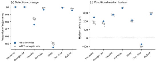
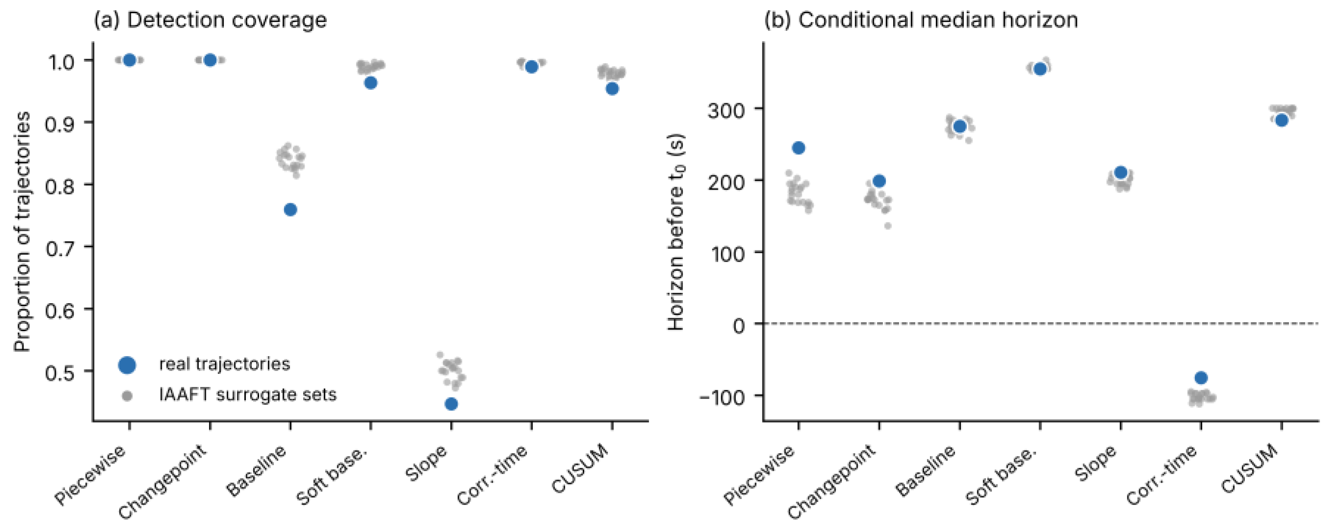
No estimator showed a statistically detectable excess of onsets in the final 150 s before t0 on real data relative to IAAFT surrogates of the same trajectories (all p ≥ 0.14; Figure 4); the largest raw difference was for CUSUM (12.7% vs. 11.1%). Coverage on real data was lower than on surrogates for the baseline (0.76 vs. 0.84), soft-baseline (0.96 vs. 0.99), slope (0.45 vs. 0.50) and CUSUM (0.95 vs. 0.98) estimators, each outside the surrogate 95% range. Conditional horizons did not differ from surrogates for the baseline (275 vs. 274 s, p = 0.62), soft-baseline (355 vs. 357 s, p = 0.86), slope (211 vs. 201 s, p = 0.19) and CUSUM (284 vs. 294 s, p = 1.0) estimators. The piecewise (245 vs. 182 s, p = 0.048) and time-correlation estimators (−76 vs. −102 s, p = 0.048) placed onsets earlier on real than on surrogate data, and changepoint showed the same tendency (199 vs. 173 s, p = 0.10); these nominal differences would not survive correction for seven comparisons and did not concentrate onsets near t0.
Figure 4.
Detection coverage (a) and conditional median horizon (b) of each estimator on the real trajectories (blue) and on 20 IAAFT surrogate sets of the same trajectories (grey), which preserve the amplitude distribution and, approximately, the power spectrum with respect to window order, but randomise the timing of changes.
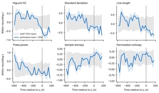
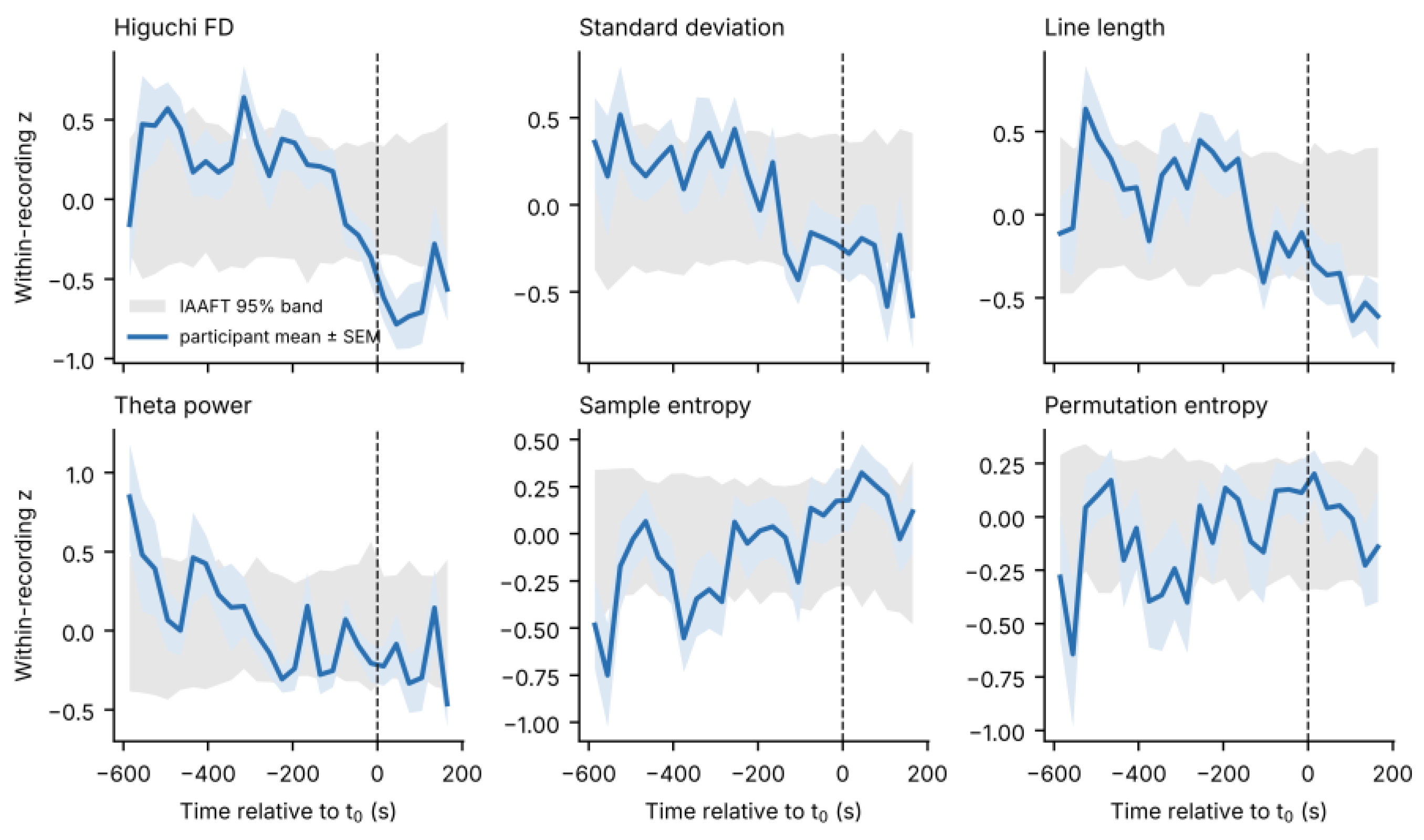
Participant-averaged trajectories showed slow monotonic trends for several features, for example a decline of Higuchi FD, standard deviation and line length and a rise in sample entropy across the window (Figure 5), but they exceeded the pointwise-surrogate band only intermittently (for example, Higuchi FD early in the window and after t0). Anchor-locked change exceeded the surrogate expectation for no feature after FDR correction (all q ≥ 0.14; 16 recordings with sufficient early windows). Uncorrected p < 0.05 was observed for decreases in alpha, delta and theta power and in peak-to-peak amplitude, minimum and maximum, whereas Higuchi FD (p = 0.40), standard deviation (p = 0.18), line length (p = 0.32) and beta power (p = 0.86) were within the surrogate range. Higuchi FD fell below the surrogate band shortly after t0, consistent with a concurrent rather than an anticipatory change; this pointwise observation is descriptive.
Figure 5.
Participant-averaged, within-recording standardised feature trajectories (blue, ±standard error of the mean (SEM); 30 s bins; n = 17 participants) aligned to t0 (dashed line). The grey band is the pointwise 95% range of the same average computed from 100 IAAFT surrogate sets.
Random displacement of the anchor by up to ±120 s did not change the method comparison (45 jittered analyses; all p < 10−7; W = 0.46–0.63), and using the alternative consensus time recorded for one session (30 s earlier) gave W = 0.54. The stability of the median horizon under this symmetric jitter is not by itself sufficient to evaluate C3. The per-trajectory analysis was informative (Table S9). In the positive control, changepoint, slope and baseline estimates stayed fixed in session time when the frame was shifted (participant-level median β = 1.00, 1.00 and 0.80), whereas soft-baseline (0.13), piecewise regression (0.14), CUSUM (0.36) and time correlation (0.41) did not, because their estimates partly follow the analysis frame. Changepoint and slope estimates also localised the injected step (median absolute error 5 and 15 s; 82% and 65% within 60 s), baseline estimates less precisely (55 s; 51%), and the other four estimators poorly (64–230 s; 12–48%). C3 can therefore be assessed only for changepoint, slope and, with less precision, baseline. In the real data, slope onsets were fixed in session time (β = 1.00, 95% CI 0.84–1.00), baseline onsets partly (0.57, 0.38–0.99), and changepoint onsets were not clearly so (0.33, −0.48 to 1.00). Tracking varied between recordings (median β −0.25 to 1.00). Being fixed in session time shows that an onset is determined by the data rather than by the frame; whether those data features relate to drowsiness is addressed by C2, which was not met.
3.5. Stability of Feature Rankings
With the corrected sample, the cross-estimator core comprised seven features (standard deviation, Higuchi FD, Katz FD, theta-to-beta ratio, line length, beta power and mean); the DFA exponent no longer met the rule. Across 27 combinations of the correlation threshold, top-N and majority rule, the core contained between 1 and 24 features; only Higuchi FD was selected under every combination. In 2000 participant-bootstrap samples, Higuchi FD (87%) and standard deviation (81%) were selected most often, whereas beta power (54%), line length (48%), Katz FD (41%), mean (27%) and theta-to-beta ratio (24%) were not; relative theta (53%) and theta power (46%), which are outside the core, were selected as often as several members (median core size 8, 95% range 5–10; median Jaccard overlap with the original core 0.33). Core membership also changed with the baseline fraction, the handling of replaced samples and the window length, whereas the method effect was preserved in every sensitivity analysis (Table 7). With 10 s and 20 s windows, coverage changed by at most 3 percentage points, conditional horizons by a median of 5–50 s per trajectory, and absolute agreement between estimators remained poor (ICC 0.04 and 0.09); Higuchi FD, line length, beta power and the mean were in the core at all three window lengths, whereas standard deviation was not selected in 10 s or 20 s windows (Table S11). Full rankings and selection frequencies are given in Tables S3 and S4.
Table 7.
Sensitivity of the method comparison (participant level) and of the cross-estimator core.
3.6. Classification Relative to Time on Task (C5)
With fully nested leave-one-participant-out validation (17 folds), the 32-feature model reached a balanced accuracy of 0.65 and an AUC of 0.65 (Table 8). Elapsed session time alone reached an AUC of 0.69, and adding it to the EEG features gave an AUC of 0.70. No improvement over the time-only model was detected (ΔAUC for EEG + time vs. time = 0.013, 95% CI −0.11 to 0.13; EEG alone vs. time = −0.03, 95% CI −0.18 to 0.09). The wide intervals do not exclude a modest gain; the analysis shows only that incremental information was not demonstrated. With nested selection the core reached a balanced accuracy of 0.62 (0.56–0.69), similar to the fixed full-cohort subset (0.62), and the nested ocular-proxy-conservative subset reached 0.64 (0.56–0.71); neither exceeded the time-only model in AUC. Within training folds, Higuchi FD, standard deviation and beta power entered the core in 17 of 17 folds and line length in 13; the conservative subset consisted of Higuchi FD (17/17), standard deviation (17/17) and line length (13/17). Full-cohort selection is retained only as a reference, because it uses the test participant.
Table 8.
Leave-one-participant-out classification (17 participants; 1128 alert, 311 drowsy windows). 95% CIs from participant bootstrap.
3.7. Consensus Detector Timing
The consensus detector departed a median of 282.5 s before t0 under retrospective localisation; the data required to confirm the departure became available a median of 22.5 s later (median 260.0 s before t0). The delay was 22.5 s in 15 recordings and 30 and 60 s in two recordings with rejected windows. With the trailing smoother the confirmation time was 283.5 s before t0 (delay of 15 s in 15 recordings; 45 and 52.5 s in two) (Table 9). The hit fraction depended on the researcher-defined tolerance window, from 0.06 (−60/+30 s) to 1.00 (−450/+60 s). Crucially, when the consensus detector was re-run around pseudo-anchors along the full sessions (16 eligible recordings), it fired before 92% of pseudo-anchors versus 94% of true anchors. The observed median lead (290 s) did not exceed the pseudo-anchor null (mean 331 s, 95th percentile 368 s; p = 0.93). With a fixed baseline of 120–240 s after session start, all 14 eligible recordings produced a detection, at a median of 416 s (range 90–1979 s) before t0. Detections typically followed shortly after the end of the baseline, whatever the anchor’s position. Individual values are given in Table S5.
Table 9.
Consensus detector timing (17 participants; lead = seconds before t0).
3.8. Source Specificity (C6)
The internal ocular proxy is, by construction, delta power. Its correlations with the other features were substantial for amplitude and low-frequency spectral measures (standard deviation r = 0.51, θ/β 0.53, DFA 0.77) and small for Higuchi FD (−0.15), line length (0.11) and beta power (0.13) (Table 10, all 32 features in Table S6). After adjustment for the proxy, partial correlations with time survived FDR correction for 15 of 32 features; they were largest for Higuchi FD (−0.50, 95% CI −0.66 to −0.29, q = 0.03), followed by standard deviation (−0.37), line length (−0.35) and the DFA exponent (0.33). These features therefore changed over the session beyond what the ocular proxy explains. Because time to t0 is a shifted copy of elapsed time within a recording, these associations cannot distinguish drowsiness from time on task. The fraction of replaced (zero-filled) samples was strongly and negatively correlated with several features within recordings: sample, fuzzy and permutation entropy (r = −0.91, −0.95 and −0.94), Petrosian FD (−0.98), zero crossings (−0.88) and line length (−0.55). It was weakly correlated with Higuchi FD (0.14) and standard deviation (−0.21). Within-recording variation in these complexity measures therefore partly reflects data replacement rather than EEG dynamics.
Table 10.
Coupling of selected features to the internal low-frequency proxy (study data) and to measured vertical EOG (external data). Participant-level mean correlations.
In the external dataset, which includes measured vertical EOG, Higuchi FD (r = 0.04) and line length (−0.15) were only weakly correlated with EOG power, whereas the DFA exponent (0.51), mean (0.50) and standard deviation (0.29) were moderately correlated, and several spectral and entropy measures were correlated with it in the negative direction (|r| 0.32–0.47). On the untransformed scale the values were similar (Higuchi FD 0.06, line length −0.19, DFA 0.41). The internal delta-band proxy correlated with measured EOG power at r = 0.55 (0.41 untransformed), but the ranking of features by proxy coupling agreed only weakly with their ranking by EOG coupling (Spearman ρ = 0.32, p = 0.08). The proxy is thus an imperfect stand-in for an EOG channel. A weak correlation with EOG does not by itself establish neural origin and does not exclude other artefacts: EMG, head motion and electrode effects were not measured in the study data and were not assessed here. Conversely, a correlation with EOG would not exclude a neural contribution, because drowsiness can change ocular and cortical activity together.
3.9. External Replication (C2, C4, C7)
In DROZY, KSS increased from 4.2 to 6.3 and 7.8 across the three test occasions, and the mean reaction time increased from 363 ms to 468 and 475 ms, confirming the sleep-deprivation manipulation. Relative to the PVT-lapse anchor, the estimator effect replicated (Friedman χ2 = 34.0, p = 6.8 × 10⁻⁶, W = 0.71; 8 participants) with a similar coverage pattern (slope 0.40, baseline 0.76, CUSUM 0.91, soft-baseline 0.96, global estimators 1.00; Table 11). Horizons were shorter than in the study data because the pre-anchor frame was truncated by the test start, and absolute agreement was again low (median pairwise difference 75 s, ICC 0.26). As in the study data, real horizons were not earlier than those of IAAFT surrogates in any estimator; in the slope estimator they were later (19 s vs. 25–52 s). No feature was associated with window-wise PVT response speed after FDR correction, either before (smallest q = 0.65) or after adjustment for elapsed time (smallest q = 0.26); all uncorrected correlations were small (|r| ≤ 0.11). With 11 participants, small associations cannot be excluded.
Table 11.
External replication in DROZY (Fz resampled to 500 Hz; same pipeline and −600/+180 s frame; 20 sessions retained, 13 with an eligible PVT-lapse anchor).
3.10. Summary Against the Interpretability Criteria
Table 12 summarises the evidence. The estimator outputs partly satisfy the precondition on anchor precision. Against an autocorrelated-noise (AR(1)) null, the conventional rules did not perform better on real data (for example, baseline coverage of 0.76 on real data vs. 0.86 on no-change simulations; Table 5 and Table 6); with design-matched null-calibrated thresholds, the baseline rule detected 25% of real trajectories, above the nominal 5% of the AR(1) reference (6% observed in the simulation check) but below the 28.5% obtained on spectrum-preserving surrogates. This comparison does not identify the source of the excess over the AR(1) reference; it only shows that the excess is not specific to the real temporal order of the data. The outputs are not anchor-specific, depend strongly on the estimator, and show no detectable gain beyond time on task. Slope onsets, and partly baseline onsets, are fixed in session time, but this criterion could not be assessed for four estimators. Source specificity was partly met, in the limited sense that Higuchi FD and line length were weakly correlated with measured EOG in an independent dataset. On this evidence, apparent pre-anchor horizons in these data correspond to evidence level 0: real coverage exceeded the AR(1) reference but not the spectrum-preserving null.
Table 12.
Evaluation of the early-onset interpretability criteria.
4. Discussion
4.1. Principal Findings
The study shows that, in two independent datasets, the time assigned to an EEG departure before drowsiness is determined mainly by the operational definition of onset. The estimators applied to identical trajectories differed by several minutes and in whether they detected anything at all (W = 0.53 and 0.71). More importantly, the same estimators reproduced the observed horizons on data that contained no anchor-related change: on autocorrelated noise, on spectrum-preserving surrogates and around pseudo-anchors. A pre-anchor horizon is therefore not, by itself, evidence of an anticipatory physiological change. This conclusion strengthens, rather than replaces, the methodological message that onset definitions shape reported biomarker timing: the definition can generate the timing.
4.2. Why Event-Based Estimators Report Early Onsets
Two mechanisms explain the null behaviour. First, a threshold applied repeatedly over many post-baseline windows is crossed by chance with high probability, and baseline statistics estimated from a short, autocorrelated segment are themselves uncertain; median smoothing increases autocorrelation further. A fixed 2 SD rule therefore behaves as a multiple-testing procedure without correction (Figure 3). Second, EEG feature trajectories contain slow drift, related to time on task, electrode settling, posture or arousal, that is not captured by short-memory noise models; in our data, 15 of 32 features changed with time beyond the ocular proxy (Section 3.8). Calibrating thresholds against autocorrelated noise removed most false onsets, but the remaining detections were matched by spectrum-preserving surrogates. A further structural factor is that the baseline, soft-baseline and CUSUM rules search only after the baseline, so their horizons are bounded by the baseline end (the slope estimator also searches within the baseline, and the time-correlation estimator has no baseline). Soft-baseline detections clustered just after it; consistent with this, soft-baseline, CUSUM, piecewise and time-correlation estimates moved partly with the analysis frame and did not fully track even an injected step (Section 3.4). Global estimators avoid this bound but always return a breakpoint, so their coverage of 100% is uninformative.
4.3. When Is an Early Onset Interpretable? Recommendations
We recommend that studies reporting EEG lead times evaluate and report the criteria in Table 2 and the items in Table 13. The minimal set is: the anchor procedure and its timing uncertainty; the exact onset rule and baseline; coverage reported jointly with conditional horizons; the estimator’s behaviour on a spectrum-preserving null (for example, IAAFT surrogates of the same trajectories) and around pseudo-anchors; a per-trajectory anchor-shift analysis with a positive control; subject-wise validation with nested feature selection and a time-only comparator; and an independent artefact channel. For threshold rules, thresholds should be calibrated to a nominal false-onset rate under a null that preserves the spectrum of the data, rather than fixed at 2 SD. The scripts implementing these benchmarks are available from the corresponding author upon reasonable request.
Table 13.
Reporting checklist for EEG onset and lead-time claims.
4.4. What the Data Do Support
Two observations survive the benchmarks, with limits. First, Higuchi FD and standard deviation were the features selected most often across estimators, folds and bootstrap samples (81–87% of bootstrap samples), whereas the remaining core members were not; Higuchi FD was also selected at all three window lengths, whereas standard deviation was not. Their ranking is therefore more stable than that of other features, although their timing is not anchor-specific. Second, Higuchi FD and line length were only weakly correlated with measured vertical EOG in an independent dataset, consistent with their small correlation with the internal proxy. A weak EOG correlation does not by itself establish neural origin and does not exclude other artefacts, because muscle, motion and electrode effects were not measured, but for single-channel frontal monitoring, where ocular contamination is a main threat, it makes these features reasonable candidates for future anchor-specific tests. Neither tracked PVT performance after correction. Conversely, the DFA exponent and amplitude measures are coupled to ocular activity at frontal sites, and entropy measures should not be computed on windows with zero-filled samples.
4.5. Relation to Previous Work
Our findings do not contradict studies that discriminate alert from drowsy states or forecast drowsiness events [7,8,9,10,11,12,13,14,15,16,17,18,19,20,21,22,23,24]. Instead, they question whether pre-event horizons obtained with onset estimators should be interpreted as anticipatory. Studies with external event definitions and multimodal sensors [20,22,23,24] are better placed to meet criteria C0 and C6, but the same null benchmarks apply to them. More generally, the problem resembles circular analysis in neuroscience, in which selection and testing on the same data inflate apparent effects [47], and the bias of cross-validation when model selection is not nested [46]. Surrogate-data testing, long established in nonlinear time-series analysis [44,45], offers a straightforward remedy.
4.6. Limitations
The study data comprise 17 participants recorded with one dry-electrode device at a single frontal site, with the same task (a monotonous driving simulation at a desk), device and electrode site in every session; the time of the session (evening or night) and its duration varied between participants, and prior sleep was instructed but not verified. This limits its power and generalisability. The anchor is an observer-verified report with about one-minute resolution, individual observer timings were not retained, and the archived video copies were in low resolution and not available for every session. No EOG, EMG, accelerometry or impedance was recorded, and the wavelet attenuation reduced blinks only partly. Samples within quality-rejected segments were zero-filled before feature computation, which affects complexity measures. Device packet jitter within a second could not be corrected. The external dataset differs in electrode (Fz), task (10 min PVT), anchor type and population, its quality-control exclusions left them with 11 participants (8 with an eligible anchor), and its 10 min tests give shorter pre-anchor frames than the study data. Non-significant results, including the absence of anchor-locked change and of a gain over elapsed time, do not establish absence; with 17 and 11 participants, small effects could be missed. Finally, all analyses are retrospective; no causal real-time system or false-alarm rate on uninterrupted recordings was evaluated.
4.7. Future Validation
A study capable of reaching evidence level three would record EOG, EMG, head motion and electrode impedance alongside frontal EEG, as in synchronous EEG–EMG acquisition for motor applications [67]. It would time the behavioural anchor on the EEG clock with inter-rater agreement, and add independent vigilance measures (PVT, KSS) at fixed intervals. Control sessions of equal duration in which participants remain alert would separate drowsiness from time on task. It would pre-register the estimator, threshold calibration and null benchmarks, and evaluate causal detectors on uninterrupted recordings with false alarms per hour. The broader project for which this work was conducted aims at drowsiness-monitoring for mining-vehicle operators; the present results indicate that such systems should be validated against these criteria before any warning lead time is claimed.
5. Conclusions
This study provides a benchmark for interpreting EEG onset times in drowsiness research. Across seven estimators and two independent datasets, the operational definition of onset determined when, and whether, a departure was detected, shifting estimates by minutes. Null benchmarks made this visible. In simulation, conventional 2 SD rules flagged onsets in most no-change trajectories. In the present recordings, no estimator showed a statistically detectable excess of onsets in the final 150 s before the anchor relative to spectrum-preserving surrogates, the consensus detector fired before pseudo-anchors as often as before the true anchor, and adding EEG features to elapsed session time gave no detectable improvement in classification. These results do not show that EEG lacks information about drowsiness; they show that, with one continuous session per participant, onset timing cannot separate drowsiness from time on task. The eight criteria, null-calibrated thresholds and reporting checklist proposed here make this distinction testable. Applying them to designs with alert control sessions, independent vigilance measures and artefact channels is the next step, and Higuchi fractal dimension and line length, which were frequently selected and only weakly correlated with measured EOG, are candidates for such anchor-specific validation.
Supplementary Materials
The following supporting information can be downloaded at: https://www.mdpi.com/article/10.3390/s26227243/s1, Table S1: recording–feature detection flags, horizons and descriptors (544 trajectories); Table S2: full simulation results; Table S3: full feature rankings per estimator; Table S4: core-selection grid and bootstrap-selection frequencies (2000 participant draws, duplicates retained as separate blocks); Table S5: individual detector timings, pseudo-anchor null and fixed-baseline results; Table S6: coupling of all 32 features to the internal proxy, time, replaced-sample fraction and measured EOG; Table S7: DROZY session summary; Table S8: sensitivity analyses; Table S9: anchor-jitter analyses, per-trajectory anchor-shift tracking slopes and positive-control step localisation; Table S10: absolute timing agreement between estimators; Table S11: window-length sensitivity.
Author Contributions
Conceptualization, B.A., A.R.R. and F.G.; methodology, B.A.; software, B.A.; validation, B.A., R.A., A.R.R. and F.G.; formal analysis, B.A.; investigation, B.A., R.A., A.R.R. and F.G.; resources, F.G.; data curation, B.A., R.A. and A.R.R.; writing—original draft preparation, B.A.; writing—review and editing, B.A., R.A., A.R.R. and F.G.; visualisation, B.A.; supervision, F.G.; project administration, B.A. and A.R.R.; funding acquisition, A.R.R. and F.G. All authors have read and agreed to the published version of the manuscript.
Funding
This research was funded by Mitacs through the Mitacs Elevate program (grant No. IT50205) and by DyMo Technology Corporation as the industry partner.
Institutional Review Board Statement
The study was conducted in accordance with the Declaration of Helsinki and approved by the Simon Fraser University Research Ethics Board (certificate No. 30000343; approval date: 20 June 2021).
Informed Consent Statement
Written informed consent was obtained from all participants before data collection.
Data Availability Statement
The EEG data of this study are available from the corresponding author upon reasonable request, subject to research-ethics and privacy requirements. The DROZY database is available from its authors under licence [48]. The analysis code, including preprocessing, feature extraction, the seven onset estimators, null benchmarks and threshold calibration, is available from the corresponding author upon reasonable request.
Acknowledgments
The authors thank the study participants and the creators of the DROZY database. During the preparation of this work, the authors used ChatGPT (OpenAI, GPT-5.6) and Claude (Claude Opus 5.5, Anthropic) for language editing, reference checking, manuscript formatting and assistance with analysis scripting. The authors specified all analyses, reviewed the code and results, and take full responsibility for the content of this article.
Conflicts of Interest
A.R.R. is affiliated with DyMo Technology Corporation. The funders had no role in the design of the study; in the collection, analyses, or interpretation of data; in the writing of the manuscript; or in the decision to publish the results. The authors declare no other conflicts of interest.
References
- Borghini, G.; Astolfi, L.; Vecchiato, G.; Mattia, D.; Babiloni, F. Measuring neurophysiological signals in aircraft pilots and car drivers for the assessment of mental workload, fatigue and drowsiness. Neurosci. Biobehav. Rev. 2014, 44, 58–75. [Google Scholar] [CrossRef] [Scilit] [PubMed]
- Papadelis, C.; Chen, Z.; Kourtidou-Papadeli, C.; Bamidis, P.D.; Chouvarda, I.; Bekiaris, E.; Maglaveras, N. Monitoring sleepiness with on-board electrophysiological recordings for preventing sleep-deprived traffic accidents. Clin. Neurophysiol. 2007, 118, 1906–1922. [Google Scholar] [CrossRef] [Scilit] [PubMed]
- Williamson, A.; Lombardi, D.A.; Folkard, S.; Stutts, J.; Courtney, T.K.; Connor, J.L. The link between fatigue and safety. Accid. Anal. Prev. 2011, 43, 498–515. [Google Scholar] [CrossRef] [Scilit] [PubMed]
- Bergasa, L.M.; Nuevo, J.; Sotelo, M.A.; Barea, R.; Lopez, M.E. Real-time system for monitoring driver vigilance. IEEE Trans. Intell. Transp. Syst. 2006, 7, 63–77. [Google Scholar] [CrossRef] [Scilit]
- Dong, Y.; Hu, Z.; Uchimura, K.; Murayama, N. Driver inattention monitoring system for intelligent vehicles: A review. IEEE Trans. Intell. Transp. Syst. 2011, 12, 596–614. [Google Scholar] [CrossRef] [Scilit]
- Lal, S.; Craig, A. Driver fatigue: Electroencephalography and psychological assessment. Psychophysiology 2002, 39, 313–321. [Google Scholar] [CrossRef] [Scilit] [PubMed]
- Lin, C.-T.; Wu, R.-C.; Liang, S.-F.; Chao, W.-H.; Chen, Y.-J.; Jung, T.-P. EEG-based drowsiness estimation for safety driving using independent component analysis. IEEE Trans. Circuits Syst. I Regul. Pap. 2005, 52, 2726–2738. [Google Scholar] [CrossRef] [Scilit]
- Awais, M.; Badruddin, N.; Drieberg, M. A hybrid approach to detect driver drowsiness utilizing physiological signals to improve system performance and wearability. Sensors 2017, 17, 1991. [Google Scholar] [CrossRef] [Scilit] [PubMed]
- Ming, Y.; Wu, D.; Wang, Y.-K.; Shi, Y.; Lin, C.-T. EEG-Based Drowsiness Estimation for Driving Safety Using Deep Q-Learning. IEEE Trans. Emerg. Top. Comput. Intell. 2021, 5, 583–594. [Google Scholar] [CrossRef] [Scilit]
- Khushaba, R.N.; Kodagoda, S.; Lal, S.; Dissanayake, G. Driver drowsiness classification using fuzzy wavelet-packet-based feature-extraction algorithm. IEEE Trans. Biomed. Eng. 2011, 58, 121–131. [Google Scholar] [CrossRef] [Scilit] [PubMed]
- Chaudhuri, A.; Routray, A. Driver fatigue detection through chaotic entropy analysis of cortical sources obtained from scalp EEG signals. IEEE Trans. Intell. Transp. Syst. 2020, 21, 185–198. [Google Scholar] [CrossRef] [Scilit]
- Chen, L.-L.; Zhao, Y.; Zhang, J.; Zou, J.-Z. Automatic detection of alertness/drowsiness from physiological signals using wavelet-based nonlinear features and machine learning. Expert Syst. Appl. 2015, 42, 7344–7355. [Google Scholar] [CrossRef] [Scilit]
- Zou, S.; Qiu, T.; Huang, P.; Bai, X.; Liu, C. Constructing multi-scale entropy based on the empirical mode decomposition (EMD) and its application in recognizing driving fatigue. J. Neurosci. Methods 2020, 341, 108691. [Google Scholar] [CrossRef] [Scilit] [PubMed]
- Jap, B.T.; Lal, S.; Fischer, P.; Bekiaris, E. Using EEG spectral components to assess algorithms for detecting fatigue. Expert Syst. Appl. 2009, 36, 2352–2359. [Google Scholar] [CrossRef] [Scilit]
- Kurt, M.B.; Sezgin, N.; Akin, M.; Kirbas, G.; Bayram, M. The ANN-based computing of drowsy level. Expert Syst. Appl. 2009, 36, 2534–2542. [Google Scholar] [CrossRef] [Scilit]
- Chuang, C.-H.; Cao, Z.; King, J.-T.; Wu, B.-S.; Wang, Y.-K.; Lin, C.-T. Brain electrodynamic and hemodynamic signatures against fatigue during driving. Front. Neurosci. 2018, 12, 181. [Google Scholar] [CrossRef] [Scilit] [PubMed]
- Min, J.; Wang, P.; Hu, J. Driver fatigue detection through multiple entropy fusion analysis in an EEG-based system. PLoS ONE 2017, 12, e0188756. [Google Scholar] [CrossRef] [Scilit] [PubMed]
- Hu, J.; Min, J. Automated detection of driver fatigue based on EEG signals using gradient boosting decision tree model. Cogn. Neurodyn. 2018, 12, 431–440. [Google Scholar] [CrossRef] [Scilit] [PubMed]
- Balam, V.P. Systematic Review of Single-Channel EEG-Based Drowsiness Detection Methods. IEEE Trans. Intell. Transp. Syst. 2024, 25, 15210–15228. [Google Scholar] [CrossRef] [Scilit]
- Nguyen, T.; Ahn, S.; Jang, H.; Jun, S.C.; Kim, J.G. Utilization of a combined EEG/NIRS system to predict driver drowsiness. Sci. Rep. 2017, 7, 43933. [Google Scholar] [CrossRef] [Scilit] [PubMed]
- Feng, X.; Guo, Z.; Kwong, S. ID3RSNet: Cross-subject driver drowsiness detection from raw single-channel EEG with an interpretable residual shrinkage network. Front. Neurosci. 2025, 18, 1508747. [Google Scholar] [CrossRef] [Scilit] [PubMed]
- Di Flumeri, G.; Ronca, V.; Giorgi, A.; Vozzi, A.; Aricò, P.; Sciaraffa, N.; Zeng, H.; Dai, G.; Kong, W.; Babiloni, F.; et al. EEG-Based Index for Timely Detecting User’s Drowsiness Occurrence in Automotive Applications. Front. Hum. Neurosci. 2022, 16, 866118. [Google Scholar] [CrossRef] [Scilit] [PubMed]
- Hassan, A.R.; Kabir, M.; Saha, S.; Keshavarz, B.; Yadollahi, A. Development of a probability model for high-resolution drowsiness detection using electroencephalogram. Sleep Med. 2026, 140, 108733. [Google Scholar] [CrossRef] [Scilit] [PubMed]
- Mora, H.J.; Echaveguren, T.; Pino, E.J. Advanced forecasting of driver drowsiness events: Non-intrusive data and multimodal BiLSTM-based modeling. Biomed. Signal Process. Control 2026, 119, 109793. [Google Scholar] [CrossRef] [Scilit]
- Stam, C.J. Nonlinear dynamical analysis of EEG and MEG: Review of an emerging field. Clin. Neurophysiol. 2005, 116, 2266–2301. [Google Scholar] [CrossRef] [Scilit] [PubMed]
- Richman, J.S.; Moorman, J.R. Physiological time-series analysis using approximate entropy and sample entropy. Am. J. Physiol. Heart Circ. Physiol. 2000, 278, H2039–H2049. [Google Scholar] [CrossRef] [Scilit] [PubMed]
- Costa, M.; Goldberger, A.L.; Peng, C.-K. Multiscale entropy analysis of biological signals. Phys. Rev. E 2005, 71, 021906. [Google Scholar] [CrossRef] [Scilit] [PubMed]
- Higuchi, T. Approach to an irregular time series on the basis of the fractal theory. Physica D 1988, 31, 277–283. [Google Scholar] [CrossRef] [Scilit]
- Hou, F.; Yu, Z.; Peng, C.-K.; Yang, A.; Wu, C.; Ma, Y. Complexity of wake electroencephalography correlates with slow wave activity after sleep onset. Front. Neurosci. 2018, 12, 809. [Google Scholar] [CrossRef] [Scilit] [PubMed]
- Bandt, C.; Pompe, B. Permutation entropy: A natural complexity measure for time series. Phys. Rev. Lett. 2002, 88, 174102. [Google Scholar] [CrossRef] [Scilit] [PubMed]
- Scheffer, M.; Bascompte, J.; Brock, W.A.; Brovkin, V.; Carpenter, S.R.; Dakos, V.; Held, H.; van Nes, E.H.; Rietkerk, M.; Sugihara, G. Early-warning signals for critical transitions. Nature 2009, 461, 53–59. [Google Scholar] [CrossRef] [Scilit] [PubMed]
- Dakos, V.; Scheffer, M.; van Nes, E.H.; Brovkin, V.; Petoukhov, V.; Held, H. Slowing down as an early warning signal for abrupt climate change. Proc. Natl. Acad. Sci. USA 2008, 105, 14308–14312. [Google Scholar] [CrossRef] [Scilit] [PubMed]
- Katz, M.J. Fractals and the analysis of waveforms. Comput. Biol. Med. 1988, 18, 145–156. [Google Scholar] [CrossRef] [Scilit] [PubMed]
- Chen, W.; Wang, Z.; Xie, H.; Yu, W. Characterization of surface EMG signal based on fuzzy entropy. IEEE Trans. Neural Syst. Rehabil. Eng. 2007, 15, 266–272. [Google Scholar] [CrossRef] [Scilit] [PubMed]
- Mizuno, T.; Takahashi, T.; Cho, R.Y.; Kikuchi, M.; Murata, T.; Takahashi, K.; Wada, Y. Assessment of EEG dynamical complexity in Alzheimer’s disease using multiscale entropy. Clin. Neurophysiol. 2010, 121, 1438–1446. [Google Scholar] [CrossRef] [Scilit] [PubMed]
- Miskovic, V.; MacDonald, K.J.; Rhodes, L.J.; Cote, K.A. Changes in EEG multiscale entropy and power-law frequency scaling during the human sleep cycle. Hum. Brain Mapp. 2019, 40, 538–551. [Google Scholar] [CrossRef] [Scilit] [PubMed]
- Goldberger, A.L.; Amaral, L.A.N.; Hausdorff, J.M.; Ivanov, P.C.; Peng, C.-K.; Stanley, H.E. Fractal dynamics in physiology: Alterations with disease and aging. Proc. Natl. Acad. Sci. USA 2002, 99, 2466–2472. [Google Scholar] [CrossRef] [Scilit] [PubMed]
- Esteller, R.; Vachtsevanos, G.; Echauz, J.; Litt, B. A comparison of waveform fractal dimension algorithms. IEEE Trans. Circuits Syst. I Fundam. Theory Appl. 2001, 48, 177–183. [Google Scholar] [CrossRef] [Scilit]
- Peng, C.-K.; Buldyrev, S.V.; Havlin, S.; Simons, M.; Stanley, H.E.; Goldberger, A.L. Mosaic organization of DNA nucleotides. Phys. Rev. E 1994, 49, 1685–1689. [Google Scholar] [CrossRef] [Scilit] [PubMed]
- Kantelhardt, J.W.; Koscielny-Bunde, E.; Rego, H.H.A.; Havlin, S.; Bunde, A. Detecting long-range correlations with detrended fluctuation analysis. Physica A 2001, 295, 441–454. [Google Scholar] [CrossRef] [Scilit]
- Kalauzi, A.; Bojić, T.; Rakić, L. Extracting complexity waveforms from one-dimensional signals. Nonlinear Biomed. Phys. 2009, 3, 8. [Google Scholar] [CrossRef] [Scilit] [PubMed]
- Lehnertz, K.; Andrzejak, R.G.; Arnhold, J.; Kreuz, T.; Mormann, F.; Rieke, C.; Widman, G.; Elger, C.E. Nonlinear EEG analysis in epilepsy: Its possible use for interictal focus localization, seizure anticipation, and prevention. J. Clin. Neurophysiol. 2001, 18, 209–222. [Google Scholar] [CrossRef] [Scilit] [PubMed]
- Muthukumaraswamy, S.D. High-frequency brain activity and muscle artifacts in MEG/EEG: A review and recommendations. Front. Hum. Neurosci. 2013, 7, 138. [Google Scholar] [CrossRef] [Scilit] [PubMed]
- Theiler, J.; Eubank, S.; Longtin, A.; Galdrikian, B.; Farmer, J.D. Testing for nonlinearity in time series: The method of surrogate data. Physica D 1992, 58, 77–94. [Google Scholar] [CrossRef] [Scilit]
- Schreiber, T.; Schmitz, A. Improved surrogate data for nonlinearity tests. Phys. Rev. Lett. 1996, 77, 635–638. [Google Scholar] [CrossRef] [Scilit] [PubMed]
- Varma, S.; Simon, R. Bias in error estimation when using cross-validation for model selection. BMC Bioinform. 2006, 7, 91. [Google Scholar] [CrossRef] [Scilit] [PubMed]
- Kriegeskorte, N.; Simmons, W.K.; Bellgowan, P.S.F.; Baker, C.I. Circular analysis in systems neuroscience: The dangers of double dipping. Nat. Neurosci. 2009, 12, 535–540. [Google Scholar] [CrossRef] [Scilit] [PubMed]
- Massoz, Q.; Langohr, T.; François, C.; Verly, J.G. The ULg multimodality drowsiness database (called DROZY) and examples of use. In Proceedings of the 2016 IEEE Winter Conference on Applications of Computer Vision (WACV), Lake Placid, NY, USA, 7–10 March 2016; pp. 1–7. [Google Scholar] [CrossRef] [Scilit]
- World Medical Association. World Medical Association Declaration of Helsinki: Ethical principles for medical research involving human subjects. JAMA 2013, 310, 2191–2194. [Google Scholar] [CrossRef] [Scilit] [PubMed]
- Dinges, D.F.; Pack, F.; Williams, K.; Gillen, K.A.; Powell, J.W.; Ott, G.E.; Aptowicz, C.; Pack, A.I. Cumulative sleepiness, mood disturbance, and psychomotor vigilance performance decrements during a week of sleep restricted to 4–5 hours per night. Sleep 1997, 20, 267–277. [Google Scholar] [CrossRef] [Scilit]
- Philip, P.; Sagaspe, P.; Moore, N.; Taillard, J.; Charles, A.; Guilleminault, C.; Bioulac, B. Fatigue, sleep restriction and driving performance. Accid. Anal. Prev. 2005, 37, 473–478. [Google Scholar] [CrossRef] [Scilit] [PubMed]
- Jasper, H.H. The ten–twenty electrode system of the International Federation. Electroencephalogr. Clin. Neurophysiol. 1958, 10, 371–375. [Google Scholar]
- Estepp, J.R.; Christensen, J.C.; Monnin, J.W.; Davis, I.M.; Wilson, G.F. Validation of a dry electrode system for EEG. In Proceedings of the Human Factors and Ergonomics Society Annual Meeting, San Antonio, TX, USA, 19–23 October 2009; Volume 53, pp. 1171–1175. [Google Scholar] [CrossRef]
- Lal, S.; Craig, A. A critical review of the psychophysiology of driver fatigue. Biol. Psychol. 2001, 55, 173–194. [Google Scholar] [CrossRef] [Scilit] [PubMed]
- Williamson, A.M.; Feyer, A.-M. Moderate sleep deprivation produces impairments in cognitive and motor performance equivalent to legally prescribed levels of alcohol intoxication. Occup. Environ. Med. 2000, 57, 649–655. [Google Scholar] [CrossRef] [Scilit] [PubMed]
- Lopes da Silva, F. EEG and MEG: Relevance to neuroscience. Neuron 2013, 80, 1112–1128. [Google Scholar] [CrossRef] [Scilit] [PubMed]
- Mitra, S.K. Digital Signal Processing: A Computer-Based Approach, 4th ed.; McGraw-Hill: New York, NY, USA, 2011. [Google Scholar]
- Kumar, P.S.; Arumuganathan, R.; Sivakumar, K.; Vimal, C. Removal of ocular artifacts in the EEG through wavelet transform without using an EOG reference channel. Int. J. Open Probl. Comput. Sci. Math. 2008, 1, 188–200. [Google Scholar]
- Donoho, D.L.; Johnstone, I.M. Ideal spatial adaptation by wavelet shrinkage. Biometrika 1994, 81, 425–455. [Google Scholar] [CrossRef]
- Petrosian, A. Kolmogorov complexity of finite sequences and recognition of different preictal EEG patterns. In Proceedings of the 8th IEEE Symposium on Computer-Based Medical Systems, Lubbock, TX, USA, 9–10 June 1995; pp. 212–217. [Google Scholar] [CrossRef] [Scilit]
- Muggeo, V.M.R. Estimating regression models with unknown break-points. Stat. Med. 2003, 22, 3055–3071. [Google Scholar] [CrossRef] [Scilit] [PubMed]
- Killick, R.; Fearnhead, P.; Eckley, I.A. Optimal detection of changepoints with a linear computational cost. J. Am. Stat. Assoc. 2012, 107, 1590–1598. [Google Scholar] [CrossRef] [Scilit]
- Truong, C.; Oudre, L.; Vayatis, N. Selective review of offline change point detection methods. Signal Process. 2020, 167, 107299. [Google Scholar] [CrossRef] [Scilit]
- Benjamini, Y.; Hochberg, Y. Controlling the false discovery rate: A practical and powerful approach to multiple testing. J. R. Stat. Soc. Ser. B (Methodol.) 1995, 57, 289–300. [Google Scholar] [CrossRef] [Scilit]
- Dinges, D.F.; Powell, J.W. Microcomputer analyses of performance on a portable, simple visual RT task during sustained operations. Behav. Res. Methods Instrum. Comput. 1985, 17, 652–655. [Google Scholar] [CrossRef] [Scilit]
- Åkerstedt, T.; Gillberg, M. Subjective and objective sleepiness in the active individual. Int. J. Neurosci. 1990, 52, 29–37. [Google Scholar] [CrossRef] [Scilit] [PubMed]
- Bibbò, L.; Laganà, F.; Pullano, S.A.; Angiulli, G. Multimodal EEG–EMG and FEM-Based Adaptive Control of Passive Upper-Limb Exoskeletons. Sensors 2026, 26, 3924. [Google Scholar] [CrossRef] [Scilit] [PubMed]

Disclaimer/Publisher’s Note: The statements, opinions and data contained in all publications are solely those of the individual author(s) and contributor(s) and not of MDPI and/or the editor(s). MDPI and/or the editor(s) disclaim responsibility for any injury to people or property resulting from any ideas, methods, instructions or products referred to in the content. |
© 2026 by the authors. Licensee MDPI, Basel, Switzerland. This article is an open access article distributed under the terms and conditions of the Creative Commons Attribution (CC BY) license.