


Abstract
Borehole strainmeters can measure deformation too small for GNSS and too slow for seismometers, but their precision transducers are complex, and this has limited them to specialized applications as either isolated instruments or sparse arrays. We developed a passive borehole areal strainmeter built with simple machining, no moving parts, and no downhole electronics to address these limitations. The sensing element is 265 m of optical fiber wound on a compliant aluminum mandrel, read as one arm of a Michelson interferometer. The Areal Optical Fiber Strainmeter (AOFS) was grouted in limestone at 28 m depth in the North Avant Field, Oklahoma, 15 m from a Gladwin Tensor Strainmeter (GTSM), and the two instruments were recorded side by side for 1579 days. Both records were calibrated against the theoretical areal strain tide with a generalized least-squares estimator that fits areal and shear couplings and a barometric admittance. The AOFS calibration is n per radian of optical phase, stationary to 0.6% over four years, with a shear leakage of 5% of the areal sensitivity. The tidally calibrated instruments agree to 1% at M2 and 2% at O1; their amplitude spectra coincide at the tidal lines and across the microseism band, where their cross spectrum has unit gain and zero phase; and with the barometric pressure removed, the GTSM spectrum lies 1.3 to 3 times above the AOFS between 1 × 10⁻⁶ and 1 × 10⁻² Hz. Above 1 Hz, the AOFS noise floor is 3 to 10 times lower than the GTSM digitizer floor, and the AOFS records a local M2.4 earthquake with 14 times lower background noise than the GTSM. The AOFS is 2.5 to 2.8 times less sensitive to barometric pressure, and its record of a 23-day water injection into a reservoir 500 m below is essentially identical to that of the GTSM. The new instrument matches the GTSM at the tides, in the microseism band, and in the injection test and has a lower noise floor above 1 Hz; it is simple to build and robust to operate, which enables a new generation of applications for borehole strainmeters.
1. Introduction
Strainmeters have been used for decades to monitor a wide range of geophysical phenomena, and recent advances in optical sensing have the potential to make these instruments accessible to a much wider range of applications. Strainmeters have measured the Earth’s free core nutation [1], volcanic processes [2], terrestrial [3,4,5] and seafloor geodesy [6], slow slip [7], and the loading from typhoons [8]. While strainmeters are typically used to explore deformations that are too small to be resolved by GNSS and too slow to be detected by broadband seismometers, several studies have shown their potential for seismological applications such as earthquake early warning [9], ground motion estimation [10], magnitude estimation [11], and source characterization [12].
These applications have employed several strainmeter technologies that can be broadly classified by their base length, the distance over which the displacement measurement is made. Long-base instruments such as free-space or evacuated-pipe laser strainmeters [13,14,15,16,17] are considered ideal for stability (drift per unit length) and calibration (the laser wavelength is the length reference). They are often deployed in tunnels or mines to avoid near-surface temperature effects because the piers that anchor their ends must follow the ground at the nanostrain level, which is difficult to achieve near the surface. Optical fiber strainmeters [18,19,20,21,22,23] were developed to avert some of the difficulties of surface laser strainmeter installations, but they suffer from the same monument stability issues [24,25,26].
Borehole strainmeters are among the most widely deployed deformation instruments because of their compact size and the mechanical and thermal stability of the borehole environment, and because grouting the instrument into the rock removes the monument problem altogether. The best known are the four-component Gladwin Tensor Strainmeter (GTSM) [27] and the single-component Sacks–Evertson dilatometer [28]. Other systems include the three-component Sacks–Evertson strainmeter [29], the YRY-2 [30] and YRY-4 [31] strainmeters, the Sakata fluid-filled [32] and interferometric [33] multi-component strainmeters, and the Ishii strain [34] and stress meters [35]. Optical versions of the short-base borehole instrument are now appearing, with interferometric displacement gauges in a six-component tensor strainmeter [36], multiplexed fiber Bragg grating Fabry–Pérot gauges [37], and Fabry–Pérot gauges embedded in a cemented sphere [38]; these replace the capacitance transducer but keep the precision-gauge architecture. These short-base instruments use very high resolution displacement transducers to measure the deformation of the down-hole package. The GTSM, for example, has a least count of strain, which for a 10 cm borehole is a displacement of m, about 50 times smaller than the Bohr radius. Achieving this precision has required advanced length metrology and specialized electronics, which has limited the application of these instruments.
The combination of this precision with a package robust enough to survive permanent installation in a borehole results in high-value instruments that are rarely abandoned after short-term studies and rarely deployed in large arrays; the six-instrument array at the Alto Tiberina Near Fault Observatory in Italy is a recent exception [39,40]. One application that needs arrays is monitoring the deformation during geologic carbon storage, where safety (the prevention of induced seismicity) and efficacy (leakage detection) can be evaluated during injection and shut-in [41,42]. The carbon storage application motivated a new generation of borehole strainmeters based on optical fiber interferometry, which leverages decades of development with commercial optical fibers and components for long-base terrestrial [18,19,20,21,22,23] and seafloor [6,43] strainmeters.
The original optical fiber borehole strainmeter concept, put forward by Frank Wyatt of the Scripps Institution of Oceanography, was a single-component instrument similar to the hydrophones developed at the Naval Research Laboratory, in which a compliant cylinder is wrapped with optical fiber [44]. The first implementation [45] was a thin-walled aluminum cylinder wrapped with fiber and sealed with epoxy to the inner diameter of a stainless steel tube that served as the pressure case. The strainmeter is grouted into an open borehole, and the length of the embedded fiber, and therefore the cross-sectional area of the borehole (the areal strain), is measured as one arm of an optical fiber Michelson interferometer. Difficulties during grouting limited the effectiveness of that first instrument, but an updated prototype at our Clemson University test site successfully measured the areal strain [41,42].
These proofs of concept led to the design of the Areal Optical Fiber Strainmeter (AOFS), which we deployed at our CO2 storage analog site in the North Avant Field north of Tulsa, Oklahoma. The AOFS was located 15 m from a GTSM [41,42], and the two instruments were recorded side by side from November 2017 to March 2022 to facilitate validation. This paper presents the design and deployment of the AOFS and the processing that turns raw optical phase into a continuous strain record. It then calibrates both instruments using Earth tides and compares the four-year drift record and the strain from the tides, barometric loading, teleseismic surface waves, a local microearthquake, and a water injection test.
2. Materials and Methods
2.1. Measurement Principle
The AOFS measures changes in the length of an optical fiber as one arm of an optical fiber Michelson interferometer. The total optical phase of coherent, monochromatic light propagating through a fiber of physical length l and refractive index n at wavelength is , so the phase difference between light returning from a sensing arm of length and a reference arm of length is
where . A change in the length of the sensing fiber, produced by a change in the circumference of the mandrel it is wound on, appears as a change in ; for the 265 m of fiber used here, one radian corresponds to of fiber strain.
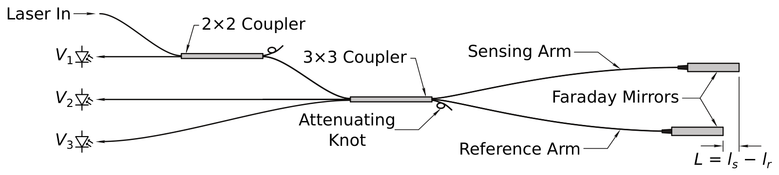
The simplest implementation of this interferometer splits the laser light into the two arms with a 2 × 2 optical fiber coupler, reflects it from a plain mirror at the end of each arm, and recombines it at the same coupler, where the two returning beams interfere. The intensity at one output of the coupler, the fringe, is , where u is the mean intensity about which the fringe oscillates (its DC level), v is the fringe amplitude, and the factor of two comes from the double pass. Two well-known problems limit this implementation [22]. Differential polarization changes in the two arms reduce the fringe contrast, and in the extreme orthogonal case, the returning beams do not interfere at all. Faraday mirrors [46] in place of the plain mirrors reflect each beam with its polarization state rotated by 90°, so that the component that traveled out on the fast axis returns on the slow axis and vice versa. The returning beams then interfere with full contrast as long as the polarization perturbations are slower than the propagation time. The other problem is that a single fringe cannot distinguish an increase in L from a decrease. A fused 3 × 3 coupler in place of the 2 × 2 splits the light three ways with a 120° phase shift between the outputs [47], so that three fringes
are available and the phase is recovered algebraically as
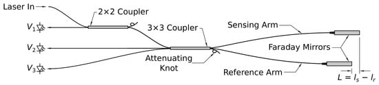
with coefficients and determined from , , and by a nonlinear least-squares fit to a known modulation [48]. Only two fringes are strictly needed [49], but the three-fringe estimate is independent of the laser power, which removes the need for active laser temperature control, a factor of three to four in field power consumption [50]. These two remedies give the topology of Figure 1: the 3 × 3 coupler splits the light into the sensing and reference arms, each ending in a Faraday mirror, and recombines it into three fringes, and a 2 × 2 coupler taps the fringe that returns toward the laser.
Figure 1.
Topology of the 3 × 3-coupler optical fiber Michelson interferometer with a 2 × 2 tap. L is the difference between the sensing () and reference () fiber lengths, and each arm ends in a Faraday mirror.
2.2. Sensing Package
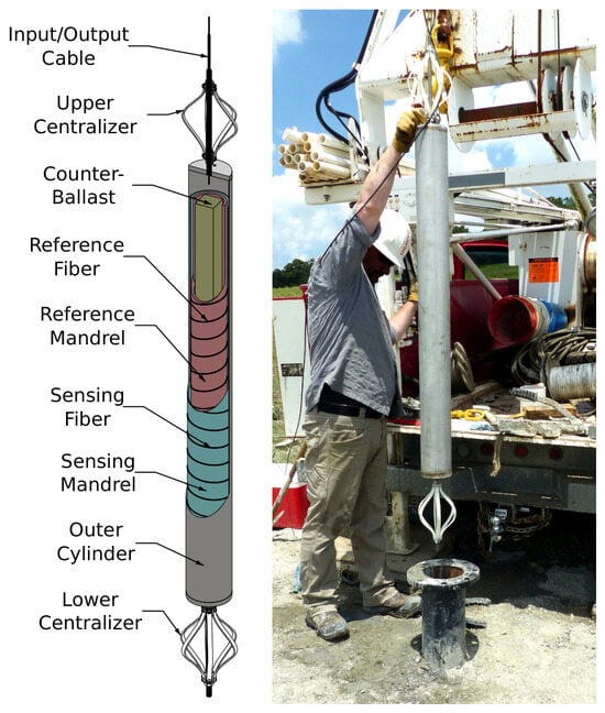
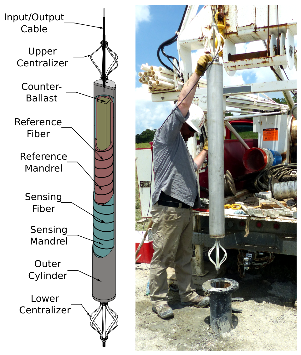
The down-hole sensing package is a set of three nested cylinders with welded end caps, centralizers, and an integrated counter-ballast bar (Figure 2). The outer cylinder protects two fiber-wrapped cylinders that house the sensing and reference arms of the interferometer. It is a standard 4-inch nominal Schedule 5 pipe of 304 stainless steel (114.3 mm diameter, 2.1 mm wall), 1.2 m long, and sealed at each end with a 12.7-mm-thick weld cap. The caps carry threaded through-holes for adjustable centralizers and lifting eyes, and the upper centralizer rod is hollow so that the main fiber cable (FBSMTACCABLE4, Fiber Instrument Sales, Oriskany, NY, USA) can pass through it.
Figure 2.
Cutaway diagram of the major AOFS components (left) and the completed instrument during installation (right).
Each arm of the interferometer is wound on one of the two inner cylinders, or mandrels. The middle cylinder is a thin-walled aluminum sleeve whose high compliance maximizes the strain transfer from the outer cylinder to the fiber. It has an outer diameter of 107 mm, a wall thickness of 2.4 mm, and a length of 1.1 m, which was turned down from a 4-inch Schedule 40 pipe. A shallow (0.3 mm) helical groove at 1.3 mm pitch (20 threads per inch) was cut into its outer surface to guide and protect the fiber. The innermost cylinder is a 3-inch nominal Schedule 80 pipe of 304 stainless steel (88.9 mm diameter, 7.6 mm wall) of the same length. Its thick wall stabilizes the reference fiber mechanically and adds weight for deployment.
The two mandrels are each wrapped with about 265 m of bend-insensitive single-mode fiber (ClearCurve ZBL, Corning, Corning, NY, USA); an optical length meter (OFLM-1000, OZ Optics, Ottawa, ON, Canada) was used to match the sensing and reference lengths to a few millimeters, so that the interferometer is nearly balanced and laser frequency noise is rejected. A 3.2-mm-wide slot cut into each cylinder 98 mm from the bottom and 24 mm from the top lets the ends of the wound fiber pass from the outer surface into the central volume. The distance between the two penetrations is 1 m, the intended sensing interval.
Assembly required care because of the fragility of the fiber and the weight of the mandrels. The sensing mandrel was set over the reference mandrel, the slots aligned, and the ends centralized and closed with epoxy about 5 mm from each end. After curing, the fiber ends were fed into the central volume and the slots were sealed to form an airtight annulus between the inner surface of the sensing mandrel and the outer surface of the reference mandrel. This air-filled annulus decouples the reference mandrel, and therefore the reference fiber, from the external strain. Faraday mirrors (FOFM-21P-1550-9/125-S-60-X-0.25-0.5, OZ Optics, Ottawa, ON, Canada) were spliced to the lower fiber ends, and 2 × 2 and 3 × 3 couplers (PSK-002121 and PSK-002122, Gould Fiber Optics, Millersville, MD, USA) were spliced to the upper ends, as shown in Figure 1. The unused port of each coupler was terminated with a tight attenuating knot, which prevents the reflection from an open fiber end from creating a parasitic interferometer. The coupler leads were spliced to the main cable and all loose fiber and components were secured to the inner surface of the reference mandrel with cyanoacrylate adhesive.
The paired mandrels were inserted into the outer cylinder together with a 50.8 mm square bar of 1018 steel for counter-ballast and volume filling, and the interior was potted in a low-exotherm, low-viscosity epoxy (Loctite Stycast 1264, Henkel, Düsseldorf, Germany) until every component was submerged. After degassing and curing, the top cap was welded on, and the remaining volume, including the annulus between the cable and the centralizer rod, was filled with epoxy. The density of the completed package is about 4.5 g/cm3, more than twice that of the grout, so it sinks and stays submerged while the grout cures.
The completed package is mechanically and operationally robust. The potted interior and welded exterior leave no seals, feedthroughs, or moving parts to fail. The package is also passive: the strain is sensed by the fiber itself, so there are no downhole electronics to be damaged by lightning, corrosion, or overheating.
2.3. Interrogator
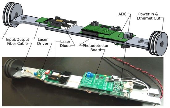
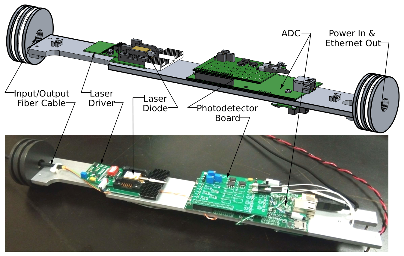
The interrogator is the active counterpart of the passive sensing package (Figure 3). It transmits coherent laser light to the down-hole optics and demodulates the returning fringes into an optical phase that is linearly proportional to the formation strain. It consists of a power distribution board, a laser driver and laser diode, a three-channel photodetector board, and an analog-to-digital converter (ADC). The power board accepts 9 to 36 V unregulated and provides regulated 5 V for the ADC and photodetectors and 12 V for the laser driver. The laser is a 1550 nm distributed-feedback diode (DFB-4G-DM-1550, Optilab, Phoenix, AZ, USA) in a 14-pin butterfly mount driven by a low-noise current source (LD1100, Thorlabs, Newton, NJ, USA). The photodetector board, developed at Clemson University, carries three InGaAs photodiodes (PD-A-25-9-1-N, Bitline System Pty. Ltd., Galston, NSW, Australia) with transimpedance amplifiers and adjustable gain, and plugs directly into a 16-bit ADC (T7 OEM, LabJack, Lakewood, CO, USA). The fringe voltages are sampled at 20 Hz and converted to phase with Equation (3) on an embedded computer, which stores the phase and the three fringe voltages in miniSEED format [51] and telemeters them to Clemson University.
Figure 3.
The Version 3 optical fiber Michelson interrogator (OFMI) with the pressure case sleeve removed: (top) CAD model with the major components labeled, from the optical fiber cable input on the left to the power and Ethernet connections on the right; (bottom) photograph of the assembled interrogator on its component tray.
All of the interrogator components are housed in a 76.2-mm-diameter, 0.5-m-long aluminum pressure case that is suspended in the borehole about 5 m below the surface. At that depth, the temperature is stable enough to run the laser without active thermal regulation, which is why the laser mount is thermally bonded to the case. The case is held over the component tray with internal snap rings so that it can be slid off with the cables attached, and the whole interrogator can be replaced without touching any up-hole or down-hole hardware.
2.4. Site and Deployment
The North Avant Field is an oil field about 50 km north of Tulsa, Oklahoma, where we have conducted water injection tests into the Bartlesville sandstone at about 530 m depth to characterize the reservoir with borehole strainmeter measurements [41,42]. A GTSM was installed in September 2016 in borehole AVN2 (36.532120° N, 96.081021° W), and the AOFS in June 2017 in borehole AVN4 (36.532109° N, 96.081199° W), 15 m away. The two borings have nearly identical completions. An air hammer drilled to 26 m, 6-inch steel casing was set, and an air rotary bit drilled the open install interval to 30 m. The install zone is a 3-m-thick limestone between 26.5 and 29.5 m in depth, bounded above and below by shale.
Both instruments were grouted in place. About 0.11 m3 of expanding grout (MasterFlow 1206, BASF, Ludwigshafen, Germany) was mixed and delivered to the bottom of the borehole with a dump bailer, giving a grout column of about 6 m, and the instrument was lowered through the grout until it was centered in the limestone. Enclosures for batteries, data acquisition, and telemetry, solar panels, and livestock fencing were installed the following day. A Vaisala WXT520 weather station at AVN4 records barometric pressure at 5 s intervals, and the GTSM carries its own 30-min barometer.
2.5. Data
The GTSM was operated by UNAVCO (now EarthScope) as Plate Boundary Observatory (PBO) station AVN2, and data from its four gauges are archived at 20 Hz and 1 Hz (network PB, channels BS1–4 and LS1–4). The AOFS phase and fringe voltages are archived at 20 Hz (network 2J, station AVN4, channel BS1), and the barometer at 0.2 Hz (channel VDO). The joint record analyzed here runs from 16 November 2017 to 12 March 2022, 1579 days. Within it the GTSM 20 Hz stream is present on 90% of days and the 1 Hz stream, which is used to bridge the 20 Hz outages, on 91%, and 1518 of the 1540 AOFS day files (98.6%) are at least 90% complete. The longest four-gauge GTSM record with no gap longer than 10 min is 432 days, from 22 August 2019 to 27 October 2020 (window WA below), during which the AOFS is 99.55% and the barometer 99.89% complete.
GTSM gauge counts were linearized with the PBO expression , with a gap g of 100 m and a borehole diameter d of 87 mm from the station metadata, which reproduces the UNAVCO Level 2 gauge strains to 0.2 n. The 20 Hz gauge streams carry two digital faults that were corrected on read: single-sample and short runs of samples 540 counts below the trace (149,343 samples on 136 gauge-days, blanked), and one 137,730-count offset on gauge 2 during 22 h in October 2021 (folded back by the exact quantum). Logger restarts hold a constant value for up to 1.5 h and were blanked, together with 60 s after each. Rare gross glitches (64 samples on 16 days, 15 million counts off on all four gauges) were blanked. No other edit was made to the GTSM record, and in particular no offsets were removed from it: the GTSM reads the displacement of its gauges since installation, so its record is continuous across power outages. Gauge 3 became intermittently noisy from mid-December 2021 to the end of the record, with ten times its usual power at periods of 30 min to 7 h; the spectral windows of Section 2.7 end before that date, and the hourly record is unaffected at the scale at which it is plotted in Section 3.4.
The AOFS optical phase is calculated as a fringe count. The instrument returns to zero at every interrogator restart, and rapid strain (a local earthquake, or the surface waves of a teleseism) can outrun the 20 Hz sampling so that whole turns of are lost or gained. Two classes of edit were therefore applied to the 20 Hz phase:
- Fringe miscounts at earthquakes. A catalog of 8799 regional and teleseismic events was screened, and for the 159 at which the AOFS phase departed from its pre-event level, the areal strain from the GTSM, converted to radians with the provisional calibration, served as a reference. A joint fit of a linear drift and an integer number of turns to the post-event difference restored 138 events (turns from to , residual after repair 0.04 rad median); 12 needed only their interior filled from the reference, 8 had no reference, and 1 needed no change. The restored events are 136 regional earthquakes of M2.5 to 4.6 at 71 to 496 km, most of them in Oklahoma, and two teleseisms, the M7.1 Ridgecrest, California, earthquake of 2019 and the M7.7 Jamaica earthquake of 2020; they occurred at 30 to 40 per year from 2018 through 2021, about one in ten of the M2.5 and larger earthquakes within 300 km.
- Offsets at restarts and tracking losses. Every remaining step was identified by eye in the full 20 Hz record and cataloged (428 events, 394 applied). The offset at each was measured by fitting 60 s lines on either side of the disturbed stretch and removed at the jump itself with a 1 s raised-cosine blend. Where the catalog bounded a burst or a tracking loss, its interior was filled with a trend or with a shape-preserving interpolant.
After these edits, the phase was scaled to strain with the calibration of Section 3.2, and the 20 Hz GTSM gauges were combined into areal strain with the tidally calibrated matrix. Both were block-averaged to 5 s and to hourly means. The offsets that remain in the hourly AOFS record were estimated against the GTSM over 48 h on either side and removed when they exceeded two standard errors. A total of 94 such offsets, mostly in 2018 and 2019 when the interrogator restarted often, were applied to the hourly and 20 Hz AOFS records. Hours during which the GTSM was settling after a restart (97 h) and AOFS warm-up hours (179 h) were dropped.
2.6. Tide Theory and Calibration Estimator
The in situ calibration of borehole strainmeters is complicated by the mismatch in stiffness between the instrument and the formation [52], by small-scale heterogeneity near the instrument [53], and by residual stresses from drilling [54]. The accepted approach is to compare the observed tidal constituents with the predicted solid Earth tide [40,55,56,57,58,59], and calibration against the dilatation of teleseismic Rayleigh waves is a recent alternative [60]. We computed the theoretical strain tensor at the site with data from the body-tide program TidalStrain.2 [61,62], ocean loading from the GOTIC2 convolution [63], and the diurnal Love-number correction for the free core nutation, and formed the areal strain and the two shears and .
Each observed hourly series was fit by generalized least squares with a model consisting of nine tidal lines (Q1, O1, P1, K1, S1, N2, M2, S2, K2), a cubic spline drift with 3-day knots, offsets at the excised episodes and gap boundaries, and the barometric pressure as a scalar regressor, with a power-law noise covariance estimated from the residuals. The series were first-differenced before fitting, which whitens the red noise; the resulting amplitudes were corrected for the differencing gain . The same design was applied to the theoretical strains, so that each observed constituent is compared with its theoretical counterpart. For each GTSM gauge i the M2 and O1 phasors were inverted for the couplings
which give the fitted areal coupling , the shear coupling , and the gauge azimuth. The pseudo-inverse of the 4 × 3 coupling matrix then yields areal strain from the four gauges; its first row is the areal calibration row, which is compared with the manufacturer’s isotropic matrix (, for every gauge, from the PBO constants and ).
The AOFS is a single channel and was fit with the single-channel form of Equation (4), , which tests whether it is purely areal: if b and c vanish, the instrument responds only to areal strain and is its calibration in n per radian. The AOFS calibration was estimated in the four windows listed in Section 3.2, of which W1, the last 391 days of the record, is the primary window; the GTSM was calibrated in W1, W0, and WA.
2.7. Spectral Estimator
Amplitude spectra and cross spectra were estimated by averaging the periodograms of many long windows of the 20 Hz records on a logarithmic frequency grid, so that a single estimator spans eight decades, from the borehole drift to the Nyquist frequency, without splicing decimated series. One hundred windows of 129 days were drawn at random starting times, with the requirements that both records be at least 98% complete and that the window end before 15 December 2021 (Section 2.5); the grout-cure trend of Section 3.4 and a straight line were removed from each window and the residual gaps were linearly interpolated. Each window was Hann tapered and transformed as a single 223-million-point FFT, and the periodogram was averaged over the FFT bins that fall in each cell of the grid, about 150 cells per decade for the spectra and 40 per decade for the cross spectra, which keeps the full resolution through the tidal bands and holds the variance of the estimate roughly constant above them. The amplitude spectra reported are the medians across the 100 windows, computed with the barometric pressure removed: for each window and instrument a frequency-independent admittance was fitted by least squares over 1 × 10⁻⁶ to 1 × 10⁻³ Hz and that multiple of the pressure record was subtracted before the periodogram was formed.
For the cross spectra of Section 3.3 and Section 3.5, the auto and cross spectra are summed over the windows and over the bins of each cell before the coherence, gain, and phase are formed. They are shown from 1 × 10⁻⁶ Hz upward, where a dozen or more independent windows contribute to every cell. Their standard errors come from a delete-one-block jackknife over the 129-day blocks in which the windows start, and the shaded bands in Figures S2, S3 and S5 are one and two standard errors. Phase is shown only where the coherence exceeds 0.2. The barometer cross spectra use 5 s means of the same windows, with the eight main tidal constituents fitted and removed from each strain window first, since the tides are incoherent with pressure and would otherwise empty the coherence across the tidal band. The cross spectrum is , so the gain is the transfer function from x to y and the phase is positive when y leads x. For the tidal lines (Section 3.5), the whole 1579-day hourly record with the tides retained was Hann tapered and transformed once; with coherent-gain normalization the periodogram then reads the constituent amplitude in nanostrain directly, and P1 and K1, 0.4% apart in frequency, are separated.
3. Results
3.1. Tidal Calibration of the GTSM
The tidal calibration of the GTSM in window WA reproduces the metadata gauge azimuths to within 1.6° using the per-gauge couplings (Table 1), and W0 and W1 agree with WA to 1 to 3% in and , so the calibration is stationary over 2019 to 2022. The fitted areal couplings, 0.42 to 0.72, are all less than the isotropic value of 0.75, and the shear couplings, 1.55 to 1.75, are all greater than 1.5. The consequence is that the manufacturer’s isotropic matrix under-reads the areal strain at this site by a factor of 1.44 at M2, whereas the tidally calibrated row reproduces the theory to 0.1% at both fitted lines and predicts the out-of-band lines N2, K1, and S2 as being 0.999, 1.008, and 0.975 of theory. Per-gauge phasors agree with the UNAVCO Level 2 metadata to a few percent in amplitude at M2 and to 5 to 9° in phase, the phase difference being the loading and reference-definition difference between the two analyses. The barometric admittance of the areal strain is n/kPa with the tidal row and n/kPa with the manufacturer’s row.
Table 1.
Per-gauge tidal calibration of the GTSM at AVN2 in window WA (22 August 2019 to 27 October 2020). and are the areal and shear couplings of gauge i in Equation (4), is the fitted azimuth clockwise from north, and the admittance is the barometric coefficient of the gauge. The manufacturer’s isotropic model has and .
3.2. Tidal Calibration of the AOFS
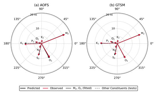
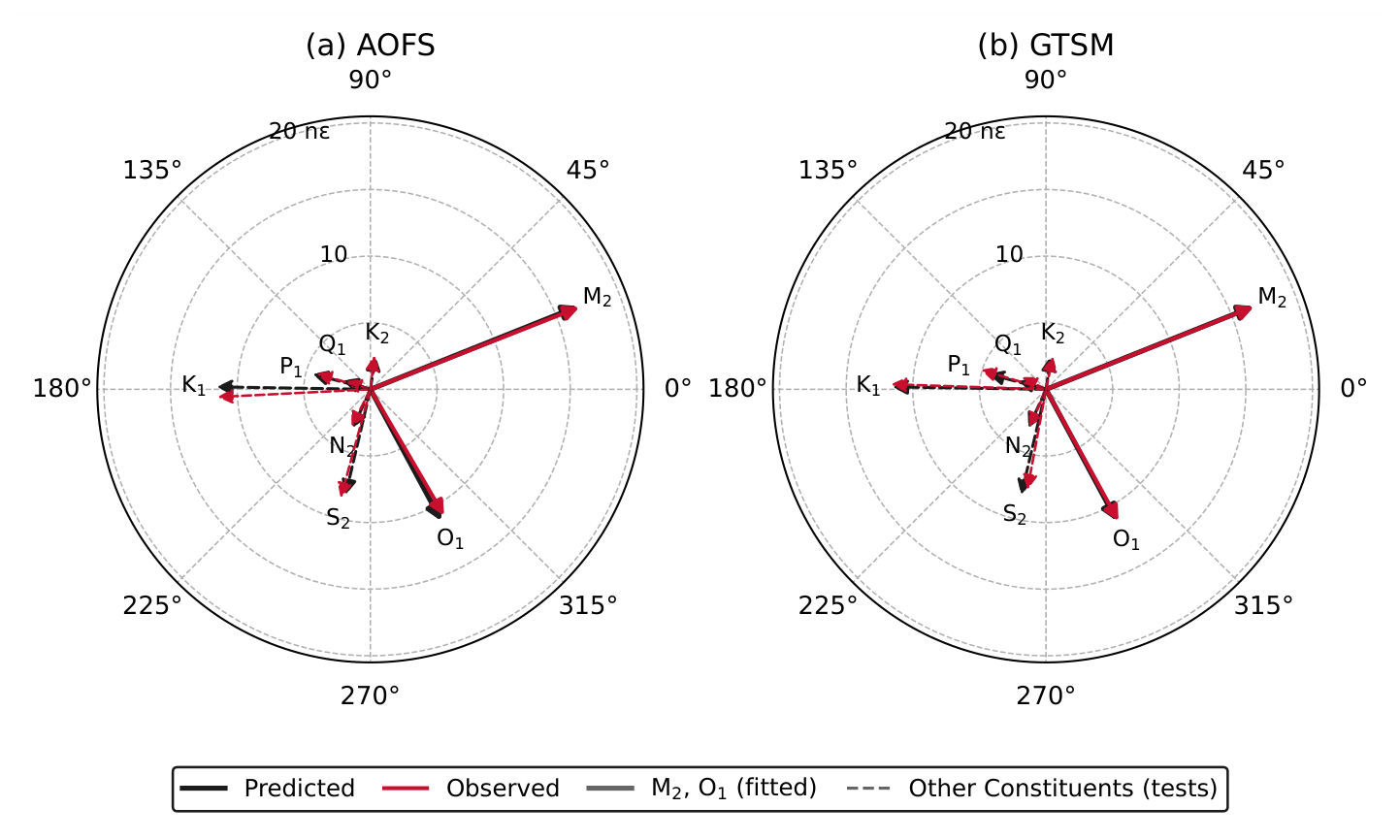
The pure-areal calibration of the AOFS is 0.2940 to 0.2958 n per radian across the four windows (Table 2), a range of 0.6% over 2018 to 2022, with 0.5 to 0.9% scatter among 90-day sub-windows; the value adopted is the W1 value, n/rad, where the uncertainty is one standard error of the fit. It does not include the uncertainty of the theoretical tide, which sets the absolute scale of the calibration: at this site, the ocean loading and the diurnal Love-number correction together change the theoretical areal tide by about 15%, and the calibration changes with it. The comparison between the two instruments does not depend on this choice, because both are calibrated against the same theory. At this scale, the nominal 16-bit least count of the interrogator is about strain. The three-coefficient fit of Equation (4) returns and in W1, a shear sensitivity of 4.4 to 5.1% of the areal sensitivity with the same sign pattern in every window (equivalent axis 14 to 33° clockwise from north). The leakage is statistically resolved ( drops from 34 to 9 in W1) but small, and the pure-areal model predicts the out-of-band lines N2, K1, K2, and S2 at 0.98, 1.00, 1.01, and 1.04 of theory as well as the four-gauge GTSM calibration does. Once each instrument is tidally calibrated against the same theory, the two instruments agree at the percent level: in W1, the M2 ratios to theory are 1.003 (AOFS) and 1.001 (GTSM), the O1 ratios are 0.976 and 0.998, and the phases agree within 2° at both lines. The observed and predicted phasor arrows (Figure 4) coincide at every constituent except S2, where the atmospheric tide adds to the solid Earth tide on both instruments, and P1 and Q1 on the GTSM, which are the weakest diurnal lines. The constituent-by-constituent amplitude ratios and phases of the AOFS fit, and the sliding 90-day calibration, are shown in Figure S1.
Table 2.
Tidal calibration of the AOFS at AVN4 in four windows. The calibration is the reciprocal of the pure-areal coupling a; the leakage is from the three-coefficient fit of Equation (4), with a, b, and c as the areal and shear couplings of the single channel; and the admittance is the barometric coefficient of the calibrated strain.
Figure 4.
Tidal phasors of the (a) AOFS and (b) GTSM areal strain in window W1: predicted from the theoretical areal strain tide (black) and observed (red) for every constituent, in nanostrain, with the phase relative to a common epoch. M2 and O1 (solid) are the constituents fitted for the calibration; the others (dashed) are predictions of the fitted model. S1 is omitted.
3.3. Barometric Admittance
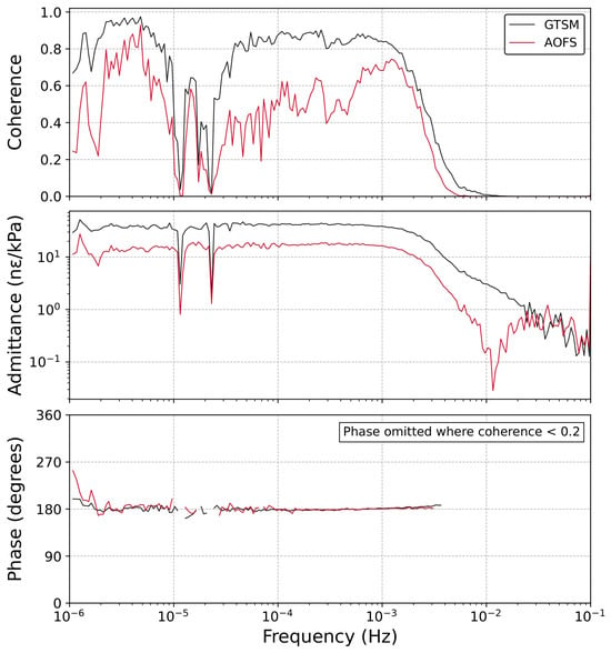
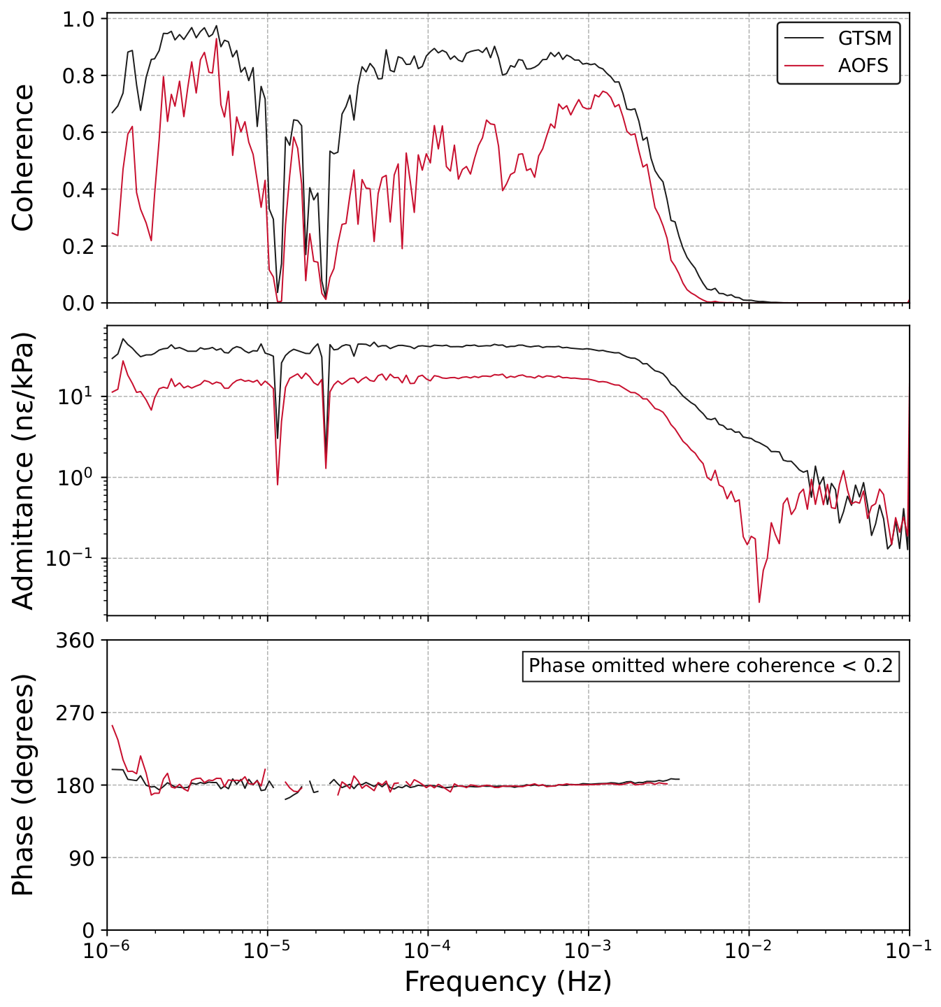
The barometric admittance of the AOFS from the tidal fits is to n/kPa depending on the window (Table 2), compared to n/kPa for the tidally calibrated GTSM areal strain and n/kPa for the manufacturer’s matrix. The AOFS is therefore 2.5 to 2.8 times less sensitive to surface loading than the GTSM. The coherence and admittance of the AOFS follow the same pattern as those of the GTSM at a smaller magnitude (Figure 5). The admittances are flat below 1 mHz, at n/kPa (GTSM) and n/kPa (AOFS), and both roll off above 2 mHz. Both strains are 180° out of phase with the pressure across the whole band in which the coherence permits a phase estimate, as expected since an increase in pressure compresses the formation. The coherence with pressure over 1 × 10⁻⁶ to 1 × 10⁻³ Hz is 0.85 for the GTSM and 0.5 for the AOFS, with a dip through the diurnal and semidiurnal bands; the lower AOFS coherence is the consequence of its smaller admittance against the same instrumental and geophysical background. The individual cross spectra with their standard-error bands are Figures S2 and S3.
Figure 5.
Median coherence, admittance, and phase between barometric pressure and areal strain for the GTSM (black) and the AOFS (red), from 100 windows of 129 days at 5 s sampling, with the tidal constituents removed from the strain. Phase is shown only where the coherence exceeds 0.2. The standard-error bands of each estimate are in Figures S2 and S3.
3.4. Time Series
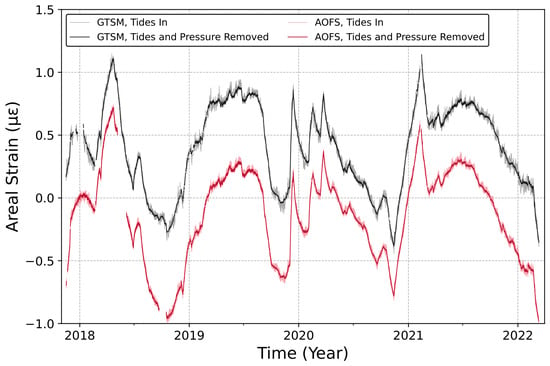
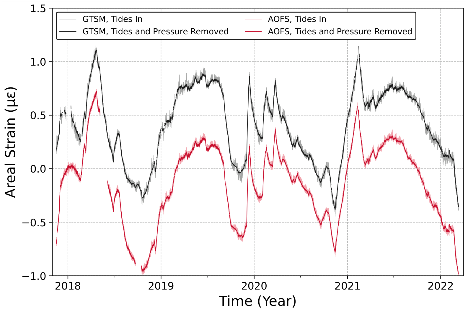
The pattern of the residual strain after the grout-cure trend is removed is nearly identical at the two instruments (Figure 6). The areal strain is characterized by annual fluctuations of about 1 peak to peak, with sharp, rapid excursions in both series caused by injection into and production from nearby wells. The slow disagreement that remains between the two records, of order 100 n over a year, is the size of the uncertainty in reconnecting the AOFS record across its interrogator restarts (Section 2.5).
Figure 6.
Hourly areal strain of the GTSM (black) and the AOFS (red) from 16 November 2017 to 12 March 2022, offset vertically for clarity. The dark traces have the tides, the barometric pressure, and the grout-cure trend removed; the light traces retain the tides. The grout-cure trend is fitted to each record, with a second exponential where needed and limited to 2000 days. The GTSM record is continuous across its outages because the gauges read displacement since installation; the AOFS record is reconnected across its interrogator restarts (Section 2.5). Positive is extension.
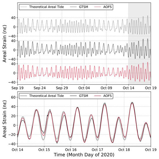
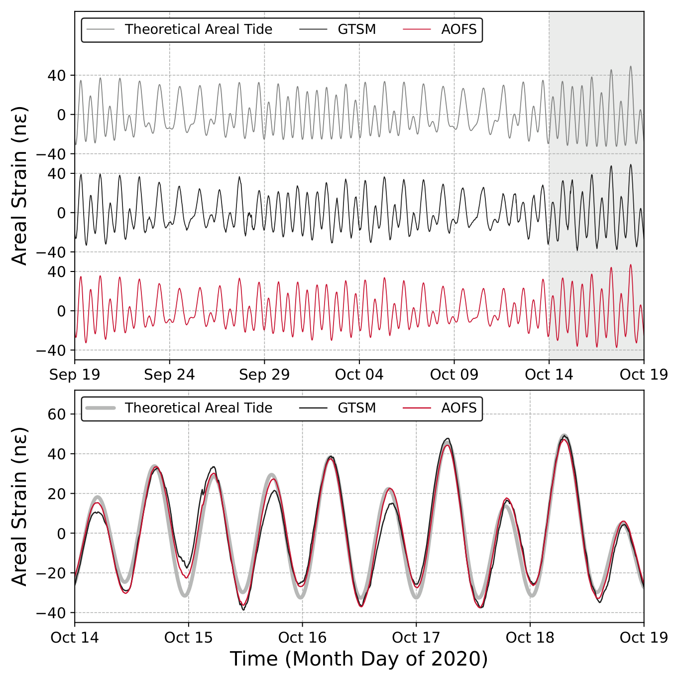
The two instruments follow each other and the theoretical areal strain tide cycle by cycle through a month that spans two spring–neap cycles (Figure 7); the rms tidal signal over the month is 17.7 n (GTSM) and 17.1 n (AOFS). Over the whole record, the M2 amplitudes read from the periodogram are 15.26 n (AOFS) and 15.48 n (GTSM), a 1.5% difference that is the O1 and M2 discrepancy of Section 3.2 averaged over the four years.
Figure 7.
Areal strain tides recorded by the GTSM (black) and the AOFS (red) and the theoretical areal strain tide (gray), 5-min means with periods longer than 2 days removed: (upper) 19 September to 19 October 2020, with the three series offset vertically; (lower) the five days of spring tides marked by the gray box, overlaid.
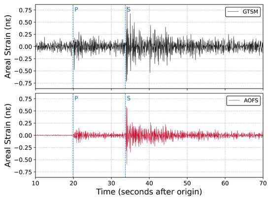
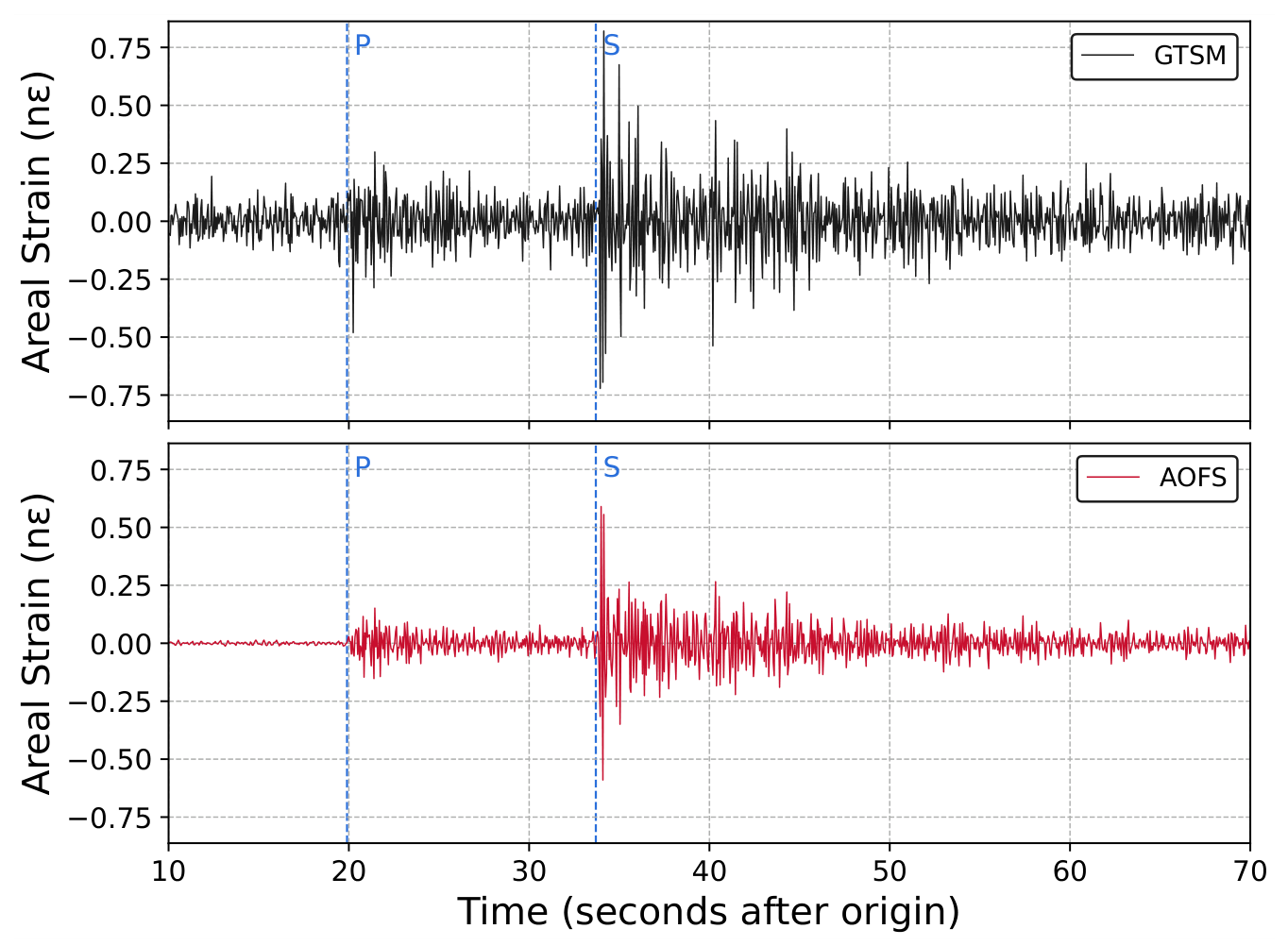
The difference in resolution between the two instruments is evident in their response to a local earthquake (Figure 8). The event is unmistakable on both instruments, with peak areal strains of 0.82 n on the GTSM and 0.59 n on the AOFS, and the two records have the same polarity and timing: over the S wave train, their correlation is 0.66 and peaks at zero lag. The background noise, however, differs by more than an order of magnitude. In the ten minutes before the origin, the rms of the high-passed GTSM record is 0.068 n, set by its digitizer, whereas that of the AOFS record is 0.005 n, a reduction by a factor of 14. The P arrival at 20 s, with a peak amplitude of 0.15 n, is clear on the AOFS record but obscured by noise on the GTSM record, which first rises above its background at the S arrival at 34 s.
Figure 8.
Areal strain from the M2.4 earthquake near Perry, Oklahoma, on 5 August 2020 (origin 11:18:34 UTC), 116 km from the site, recorded at 20 Hz by the GTSM (upper) and the AOFS (lower), high-passed at 1 s and plotted at the same scale. The dashed lines mark the P and S arrivals. The pre-event rms is 0.068 n on the GTSM and 0.005 n on the AOFS.
At the other end of the seismic band, where both instruments are far above their noise floors, the two records agree. The surface waves of the M8.2 Chignik, Alaska, earthquake of 29 July 2021, 5030 km from the site, are compared in Figure S4. The peak areal strains are 222 n (GTSM) and 204 n (AOFS), and the root-mean-square difference between the two traces over the two hours is 2.6 n, about 1% of the peak.
3.5. Spectra and Cross Spectra
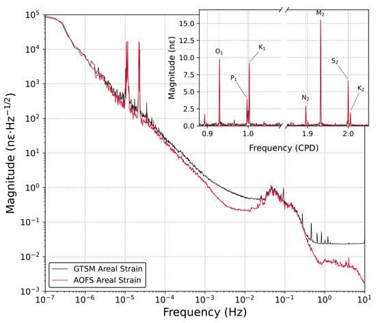
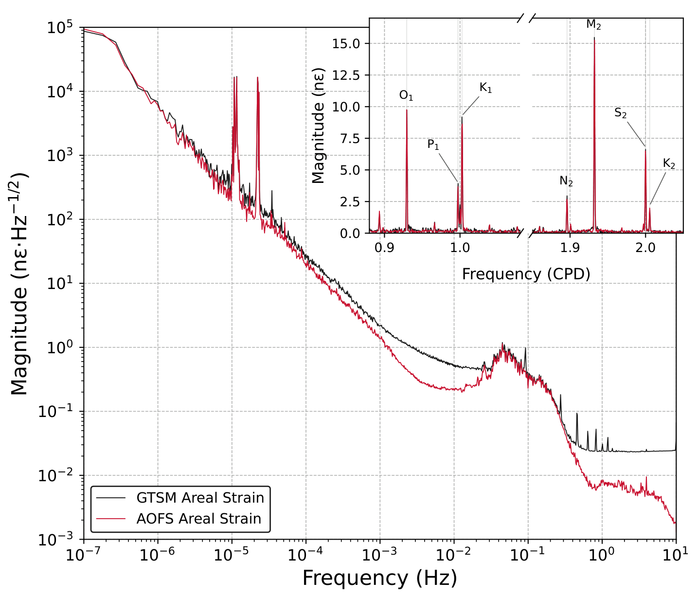
The median amplitude spectrum of the AOFS is less than or equal to that of the GTSM across eight decades of frequency, from 1 × 10⁻⁷ Hz to the 10 Hz Nyquist frequency (Figure 9). The two spectra coincide below 1 × 10⁻⁶ Hz, at the tidal lines (within 4% at O1, K1, M2, and S2), and from 0.03 to 0.3 Hz through the microseism peak near 0.05 Hz (about 1 n·Hz−1/2), where the GTSM is higher by 5 to 10%. Between 1 × 10⁻⁶ and 1 × 10⁻³ Hz, the GTSM spectrum lies 1.3 to 1.5 times above the AOFS spectrum, and between 1 × 10⁻³ and 1 × 10⁻² Hz, the excess grows to a factor of 2 to 3, a broad shoulder in the GTSM spectrum that the AOFS does not share. The spectra diverge again above 0.3 Hz, where the GTSM reaches a white floor of n·Hz−1/2 with tones at 0.44, 0.75, 1, 2, 3, and 4 Hz, while the AOFS continues to fall from at 0.5 Hz to at 1 Hz and n·Hz−1/2 at 8 Hz, 3 to 10 times below the GTSM between 1 and 8 Hz (both spectra roll off toward the Nyquist frequency with the acquisition filters). At the low end, both spectra rise to about n·Hz−1/2 at 1 × 10⁻⁷ Hz, which is the wander of the borehole rather than instrument noise, since the two records agree there in the time domain. In the inset, the seven tidal lines from O1 to K2 appear at the same amplitudes on both instruments, and P1 and K1 are resolved.
Figure 9.
Median amplitude spectra of the GTSM (black) and the AOFS (red) areal strain over 100 windows of 129 days at 20 Hz, with the barometric pressure removed from both records. The inset shows the diurnal and semidiurnal tidal bands, with the frequency axis broken between them, from the whole-record hourly periodogram in nanostrain of constituent amplitude, with the constituents O1, P1, K1, N2, M2, S2, and K2 marked.
The cross spectrum between the two records (Figure S5) quantifies their similarity. The gain of the AOFS relative to the GTSM is 0.97 to 1.03 at the tidal lines, where the coherence is 0.93 to 1.00, and 0.94 across the microseism band, where the coherence reaches 0.99 and the phase is zero. Between 1 × 10⁻⁶ and 1 × 10⁻³ Hz, with the tidal lines excepted, the gain is 0.4 and the coherence 0.65 (0.8 below 1 × 10⁻⁵ Hz). This is the band in which barometric loading dominates both records. The two instruments, calibrated to agree on the tides, respond differently to surface loading. Between 1 × 10⁻³ and 1 × 10⁻² Hz, the coherence is 0.66 while the gain stays at 0.4, so the GTSM shoulder of Figure 9 is mostly power that the AOFS does not see. Above 0.3 Hz, the coherence falls below 0.2 as the GTSM digitizer noise takes over.
3.6. Water Injection Test
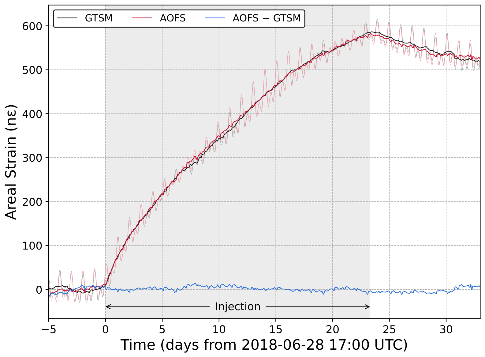
We have performed several water injection tests into the Bartlesville sandstone to induce strains and pressure changes that characterize the reservoir [41,42]. In the test analyzed here, water was injected into well 9A, about 220 m from the strainmeters and completed at about 530 m depth, for 23.3 days from 17:00 UTC on 28 June 2018 at an average rate of m3/s (450 barrels per day). The tides, the barometric pressure, and the grout-cure trend were removed from both records. The linear drift that remains was removed from the GTSM record with a line fitted to the week before injection, and from the AOFS record with a line fitted jointly with the amplitude ratio of the two records over the whole window.
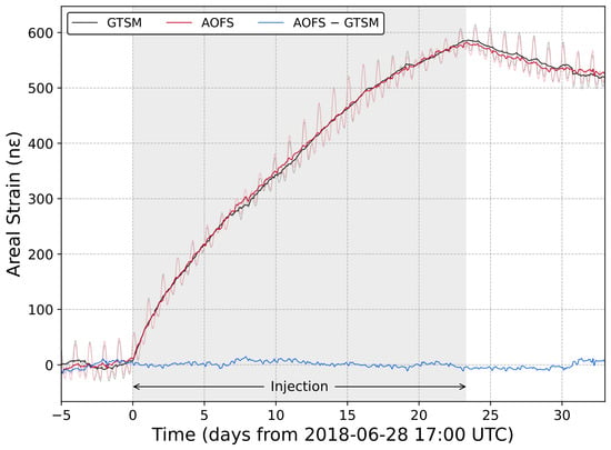
The areal strain increased within an hour of the start of injection, and the records of the two instruments are nearly indistinguishable (Figure 10). The strain rate decreased during the injection, which gives the records their negative curvature, up to a maximum strain of 584 n (GTSM) and 576 n (AOFS) at the end of injection. The strain decreased slightly after injection, and the records from the two instruments are essentially the same over the 33-day comparison. The rms difference between them during the injection is 4.4 n, and the amplitude ratio of the AOFS to the GTSM is .
Figure 10.
Areal strain recorded by the GTSM (black) and the AOFS (red) during water injection into well 9A (gray box, 28 June to 22 July 2018), hourly means with the tides, barometric pressure, and borehole drift removed, and their difference (blue). The series with the tides retained are shown in light gray and light red for scale.
4. Discussion
The AOFS matches the GTSM everywhere the two can be compared, and exceeds it at high frequency. Both instruments respond to the tides at the theoretical amplitude, their amplitude spectra coincide at the tidal lines and across the microseism band, and their cross spectrum has unit gain and zero phase there (Figure 9 and Figure S5). Between 1 × 10⁻⁶ and 1 × 10⁻² Hz, the GTSM spectrum lies above the AOFS spectrum, but we do not interpret this as lower instrument noise in the AOFS: the excess is consistent with loads that the barometer does not capture, to which the GTSM is more sensitive, and in this band, we claim only that the two instruments agree where they are coherent. Above 1 Hz, the AOFS noise floor is set by the interferometer and continues to fall to 10 Hz, whereas the GTSM is limited by its digitizer, which gives the AOFS 14 times lower background noise at the periods of local earthquakes. This is the first optical fiber borehole strainmeter to reach the performance of the GTSM, and it does so with a sensing package made from standard materials with simple machining and no seals, feedthroughs, or moving parts.
The AOFS differs from the earlier optical fiber strainmeters in terms of where the fiber is and what it measures. The terrestrial instruments stretch fiber between anchors tens to hundreds of meters apart, horizontally at the surface [18,21,23] or vertically between the surface and a point at depth [19,20,22,64], and the seafloor instruments do the same between seafloor monuments [6,43]. Their sensitivity comes from the length of the baseline, and their stability depends on the anchors, as for any long-base strainmeter. The AOFS winds 265 m of fiber into a 1.2 m package grouted in a borehole, so it measures the deformation of the borehole as the GTSM does and needs no monuments; the length of the wound fiber supplies the sensitivity that the baseline supplies in the long-base instruments. The earlier borehole implementations of this concept [41,42,45] measured the areal strain but were not compared over long records with a co-located instrument, and to our knowledge, the record presented here is the first multi-year evaluation of an optical fiber borehole strainmeter against a GTSM.
One difference between the two instruments is the barometric admittance (Table 2 and Figure 5). The AOFS responds to barometric loading with 2.5 to 2.8 times less strain per kilopascal than the GTSM, both from the tidal fits and from the cross spectra over the whole loading band, even though the two instruments agree on the tides and on the injection test. We attribute the difference to the vertical stress. The tides and the injection strain the formation at the instruments under essentially zero vertical stress, because the free surface is 28 m above, and the tidal calibration sets the response of each instrument to that kind of strain. A load on the surface changes the vertical stress, and the response of a borehole strainmeter to vertical stress depends on the vertical compliance of its package, which the tidal calibration does not constrain [55] and which varies from site to site and with frequency [65]. The thick-walled reference mandrel, the steel ballast bar, and the fully potted interior make the AOFS much stiffer axially than the GTSM, whose gauges are hollow thin-walled cylinders, so the AOFS converts less of the vertical stress into a signal. A quantitative estimate of the two vertical compliances would require the internal construction of the GTSM gauges and a numerical model of each package in its grout column, which are beyond the scope of this paper; the measured ratio of the admittances, 2.5 to 2.8, is the empirical measure of the difference. The 0.4 gain of the AOFS relative to the GTSM between 1 × 10⁻⁶ and 1 × 10⁻² Hz (Figure S5) is the ratio of the two admittances, and the same coupling is the likely reason the GTSM spectrum stays 1.3 to 1.5 times above the AOFS spectrum between 1 × 10⁻⁶ and 1 × 10⁻³ Hz after the pressure is removed (Figure 9): whatever surface loading the barometer does not capture, such as rainfall and soil moisture, acts on the GTSM with the same larger admittance. Other contributions that a single site cannot exclude are differences in the grout coupling of the two instruments and in the near-borehole stress state at their locations 15 m apart; a comparison at a second site would separate them from the package response. The GTSM shoulder between 1 × 10⁻³ and 1 × 10⁻² Hz is a separate question. Its coherence with the barometer falls to 0.05 above 3 mHz, so it is not barometric loading, and its coherence with the AOFS is 0.66 at the same 0.4 gain, so part of it is ground motion that both instruments record and the rest is unexplained.
The other difference is the shear leakage (Table 2). The AOFS is designed to be purely areal, and the three-coefficient tidal fit resolves a shear sensitivity of 4.4 to 5.1% of the areal sensitivity with a stable orientation. Since the fiber is wound uniformly around the mandrel, a shear response requires an azimuthal asymmetry in the coupling, which could be caused by the borehole, the grout column, or the off-center counter-ballast bar. The leakage is small enough to ignore for most applications, and it can be removed with the fitted coefficients when the shear strains are known.
The main limitation of the AOFS as deployed is the fringe count. The interrogator returns to zero at every restart, and rapid strain can outrun the 20 Hz sampling, so the record had to be reconnected at 394 cataloged offsets and 138 earthquake miscounts, with the nearby GTSM serving as the reference. The two kinds of offset have different remedies. The miscounts occur when the strain rate outruns the fringe tracking, and later interrogators built on this design eliminate them by oversampling the fringes and by counting quarter fringes with a high-rate digital comparator. The restart offsets are a harder problem. While the interrogator is off, the strain continues to change, and recovering the change requires an absolute measurement of the fiber length at a resolution comparable to a fraction of a fringe. Techniques that approach this resolution are not yet practical for an autonomous, low-power field instrument, and those that are practical lack the resolution, so this remains an open problem for interferometric optical fiber strainmeters in general. Until it is solved, an outage leaves an offset that must be estimated, either from a nearby instrument, as was done here with the GTSM, or from the model of the borehole drift that every strainmeter record already requires. The reconnection uncertainty, of order 100 n per year, sets the limit on the long-period comparison in Figure 6 and is the reason the lowest decade of the spectra reflects the borehole rather than the instruments. The other comparisons do not depend on the reconnection: the tidal calibration is made on first-differenced hourly series, in which a reconnection error is a single outlier, and the two earthquakes and the injection test fall between restarts.
The motivation for this instrument was the need for an array. The borehole strainmeters described in the Introduction are built one at a time around precision displacement transducers, and this level of effort has limited their applications to single instruments or sparse arrays of a few. Many important applications for strainmeters involve monitoring subsurface systems that are spatially distributed, such as reservoirs, volcanoes, hydraulic fractures, and aquifers. Resolving distributions of pressure, temperature, or properties in the subsurface from strain data is best served by an array of instruments, which has been impractical with earlier designs. The same economics drive the move to passive optical sensors with shared up-hole electronics for seafloor arrays [66] and the low-cost optical borehole strainmeters now under development [37,38]. The AOFS removes the specialized components used in earlier instruments. The sensing element is fiber wound on tubing, the package is welded and potted in epoxy with no feedthroughs or moving parts, and the interrogator is an up-hole unit that can be exchanged while the downhole sensor remains in place. Building an array then becomes a matter of drilling, grouting, and calibrating the instruments in the field.
Many of the applications that need arrays need only the areal strain. A volumetric source at depth, such as injection into or withdrawal from a reservoir, produces an areal strain at the strainmeter whose onset and shape carry information about the hydraulic diffusivity of the formation. Leak detection and induced-seismicity monitoring rest on the same areal or volumetric signal. Some important characteristics, such as reservoir boundaries, can be evaluated with shallow areal strain data from several locations. Similar results can be achieved with fewer tensor strainmeters [67,68], but this is a difference in degree, not in kind, and the simple, high-performance strainmeter described here has a place in subsurface characterization and monitoring.
The AOFS also demonstrates the performance of a new sensor design. The fiber-wound mandrel, the potted and welded package, the three-fringe interrogation, and the in situ calibration are the elements of a package that holds several fiber elements at different azimuths; the configuration required to measure the horizontal strain tensor and tensor instruments built from these elements have been deployed in Oklahoma and Utah [69,70]. The results presented here establish the performance of a one-component instrument against the GTSM, and the multi-component instruments are now being evaluated in the field.
5. Conclusions
We have developed and described a borehole areal strainmeter that uses an embedded optical fiber as a passive sensing element and have compared it over four years with data from a co-located Gladwin Tensor Strainmeter. The two instruments agree to 1% at M2 and 2% at O1, and the AOFS calibration of n per radian is stationary to 0.6% over 2018 to 2022. The amplitude spectra coincide at the tidal lines and across the microseism band, and above 1 Hz, the AOFS is 3 to 10 times quieter, with a 16-bit least count of strain. The instrument is 2.5 to 2.8 times less sensitive to barometric loading than the GTSM, which points to a lower vertical coupling of the potted, ballasted package, and it records the strain of a reservoir injection test at the same amplitude as the GTSM (). The AOFS is built from readily available materials with simple machining and is straightforward to assemble, in contrast to every other strainmeter of comparable resolution, and it needs no precision transducer and is calibrated in place against the tides, which makes dense borehole strain arrays practical. Multi-component embedded optical fiber strainmeters that resolve the full horizontal strain tensor are now being built on the same principle.
Supplementary Materials
The following supporting information can be downloaded at https://www.mdpi.com/article/10.3390/s26227154/s1. Figure S1: Tidal calibration of the AOFS in window W1; Figure S2: Coherence, admittance, and phase between the barometric pressure recorded at AVN4 and the AOFS areal strain, from 5 s means; Figure S3: As Figure S2, for the GTSM areal strain from the tidally calibrated four-gauge combination; Figure S4: Areal strain from the M8.2 Chignik, Alaska, earthquake of 29 July 2021 (origin 06:15:49 UTC, 5030 km from the site) recorded by the GTSM (upper) and the AOFS (lower), 1 s means of the 20 Hz records band-passed between 10 and 100 s; Figure S5: Coherence, gain, and phase of the AOFS areal strain relative to the GTSM areal strain from the 20 Hz records, 1 × 10⁻⁶ to 10 Hz, with one and two standard-error bands.
Author Contributions
Conceptualization, S.D. and L.C.M.; methodology, S.D.; software, S.D.; validation, S.D.; formal analysis, S.D.; investigation, S.D. and L.C.M.; resources, L.C.M.; data curation, S.D.; writing—original draft preparation, S.D.; writing—review and editing, S.D. and L.C.M.; visualization, S.D.; supervision, L.C.M.; project administration, L.C.M.; funding acquisition, L.C.M. All authors have read and agreed to the published version of the manuscript.
Funding
This research was funded by the United States Department of Energy, National Energy Technology Laboratory, under award number DE-FE0023313. The APC was funded by Tensora, Inc.
Institutional Review Board Statement
Not applicable.
Informed Consent Statement
Not applicable.
Data Availability Statement
All data are publicly available through the EarthScope Consortium data services: the optical fiber areal strainmeter (network 2J, station AVN4, location P1, channel BS1), the Gladwin tensor strainmeter (network PB, station AVN2, location T0, channels BS1–4 and LS1–4), and the barometric pressure (network 2J, station AVN4, location M1, channel VDO). The station pages at the EarthScope (formerly IRIS) Data Management Center are https://ds.iris.edu/mda/PB/AVN2/ (accessed on 9 November 2026) and https://ds.iris.edu/mda/2J/AVN4/ (accessed on 9 November 2026). The UNAVCO Level 2 processing metadata for AVN2 are available at http://bsm.unavco.org/bsm/level2/osageavn2bok2016/ (accessed on 9 November 2026). The edit catalogs, calibration tables, and processing scripts used in this paper are available from the corresponding author.
Acknowledgments
We thank Leonid Germanovich of Clemson University and Marvin and Scott Robinowitz of Grand Resources for access to, and logistical support at, the North Avant Field. Wade Johnson, Mike Gottlieb, Liz Van Boskirk, Kathleen Hodgkinson, and Charlie Sievers of UNAVCO; Matt Seigler of Clemson University; John Hu of the Georgia Institute of Technology; and Rob Moak of Tensora, Inc. helped us in the field. Machining was done by Clemson University Machining and Technical Services, and the borings were drilled by Two Eight Drilling of Tahlequah, Oklahoma. The views and opinions expressed herein are those of the authors and do not necessarily state or reflect those of the United States Government or any agency thereof. During the preparation of this manuscript, the authors used Claude Code (Anthropic, San Francisco, CA, USA) with the Claude Opus 5.5 and Claude Fable 5.1 models to assist with drafting and editing the text, auditing the data-processing and figure scripts, and checking the bibliography. The authors have reviewed and edited all output and take full responsibility for the content of this publication.
Conflicts of Interest
S.D. is a co-founder and the Chief Technology Officer of Tensora, Inc., which commercializes borehole strainmeters derived from the design described here. The instrument, the field work, and the data were developed and collected at Clemson University before Tensora existed, and the analysis and writing were carried out by S.D. independently of, and without funding from, Tensora, which had no role in the design of the study or in the collection, analysis, or interpretation of data. Tensora funded the article processing charge. L.C.M. declares no conflicts of interest. The research funders had no role in the design of the study; the collection, analysis, or interpretation of data; the writing of the manuscript; or the decision to publish the results.
Abbreviations
The following abbreviations are used in this manuscript:
| ADC | Analog-to-digital converter |
| AOFS | Areal Optical Fiber Strainmeter |
| CAD | Computer-aided design |
| FFT | Fast Fourier transform |
| GNSS | Global navigation satellite system |
| GTSM | Gladwin Tensor Strainmeter |
| OFMI | Optical fiber Michelson interrogator |
| PBO | Plate Boundary Observatory |
| rms | Root mean square |
| UNAVCO | University NAVSTAR Consortium (now EarthScope Consortium) |
References
- Amoruso, A.; Crescentini, L. Parameters of the Earth’s Free Core Nutation from Diurnal Strain Tides. Sci. Rep. 2020, 10, 9756. [Google Scholar] [CrossRef] [Scilit] [PubMed]
- Bonaccorso, A.; Currenti, G.; Linde, A.; Sacks, S.; Sicali, A. Intrusive, explosive and effusive processes as revealed by the borehole dilatometer network on Mt. Etna volcano. Front. Earth Sci. 2019, 7, 357. [Google Scholar] [CrossRef] [Scilit]
- Bohnhoff, M.; Dresen, G.; Ceken, U.; Kadirioglu, F.T.; Kartal, R.F.; Kilic, T.; Nurlu, M.; Yanik, K.; Acarel, D.; Bulut, F. GONAF–the borehole Geophysical Observatory at the North Anatolian Fault in the eastern Sea of Marmara. Sci. Drill. 2017, 22, 19–28. [Google Scholar] [CrossRef] [Scilit]
- Zhu, K.; Chi, C.; Yu, Z.; Fan, M.; Li, K.; Sun, H. The characteristics analysis of strain variation associated with Wenchuan earthquake using principal component analysis. Ann. Geophys. 2020, 63, 549. [Google Scholar] [CrossRef] [Scilit]
- Hanagan, C.; Bennett, R.A.; Barbour, A.; Hughes, A.N. Afterslip and creep in the rate-dependent framework: Joint inversion of borehole strain and GNSS displacements for the Mw 7.1 Ridgecrest earthquake. J. Geophys. Res. Solid Earth 2024, 129, e2024JB028908. [Google Scholar] [CrossRef] [Scilit]
- Zumberge, M.A.; Hatfield, W.; Wyatt, F.K. Measuring seafloor strain with an optical fiber interferometer. Earth Space Sci. 2018, 5, 371–379. [Google Scholar] [CrossRef] [Scilit]
- Zali, Z.; Martínez-Garzón, P.; Mencin, D.; Beroza, G.C. Slow slip modulates low-frequency seismicity on the Parkfield segment of the San Andreas Fault. Nat. Commun. 2026, 17, 5137. [Google Scholar] [CrossRef] [Scilit] [PubMed]
- Mouyen, M.; Canitano, A.; Chao, B.F.; Hsu, Y.J.; Steer, P.; Longuevergne, L.; Boy, J.P. Typhoon-induced ground deformation. Geophys. Res. Lett. 2017, 44, 11,004–11,011. [Google Scholar] [CrossRef] [Scilit]
- Farghal, N.; Barbour, A.; Langbein, J. The potential of using dynamic strains in earthquake early warning applications. Seismol. Res. Lett. 2020, 91, 2817–2827. [Google Scholar] [CrossRef] [Scilit]
- Farghal, N.; Baltay, A.; Langbein, J. Strain-Estimated Ground Motions Associated with Recent Earthquakes in California. Bull. Seismol. Soc. Am. 2020, 110, 2766–2776. [Google Scholar] [CrossRef] [Scilit]
- Barbour, A.J.; Langbein, J.O.; Farghal, N.S. Earthquake magnitudes from dynamic strain. Bull. Seismol. Soc. Am. 2021, 111, 1325–1346. [Google Scholar] [CrossRef] [Scilit]
- Barbour, A.J.; Crowell, B.W. Dynamic strains for earthquake source characterization. Seismol. Res. Lett. 2017, 88, 354–370. [Google Scholar] [CrossRef] [Scilit]
- Berger, J.; Lovberg, R.H. Earth Strain Measurements with a Laser Interferometer: An 800-meter Michelson interferometer monitors the earth’s strain field on the surface of the ground. Science 1970, 170, 296–303. [Google Scholar] [CrossRef] [Scilit] [PubMed]
- Jahr, T.; Kroner, C.; Lippmann, A. Strainmeters at Moxa observatory, Germany. J. Geodyn. 2006, 41, 205–212. [Google Scholar] [CrossRef] [Scilit]
- Garoi, F.; Apostol, D.; Damian, V.; Logofătu, P.C.; Ioniţă, B.F.; Lazar, J.; Molesini, G.; Papadopoulos, T.; Ionescu, C.; Ţugui, A. CALAS: Carpathian laser strainmeter: A project and preliminary results. In Advanced Laser Technologies 2007; International Society for Optics and Photonics: Bellingham, WA, USA, 2008; Volume 7022, p. 702218. [Google Scholar] [CrossRef] [Scilit]
- Milyukov, V.; Kopaev, A.; Zharov, V.; Mironov, A.; Myasnikov, A.; Kaufman, M.; Duev, D. Monitoring crustal deformations in the Northern Caucasus using a high precision long base laser strainmeter and the GPS/GLONASS network. J. Geodyn. 2010, 49, 216–223. [Google Scholar] [CrossRef] [Scilit]
- Araya, A.; Takamori, A.; Morii, W.; Miyo, K.; Ohashi, M.; Hayama, K.; Uchiyama, T.; Miyoki, S.; Saito, Y. Design and operation of a 1500-m laser strainmeter installed at an underground site in Kamioka, Japan. Earth Planets Space 2017, 69, 77. [Google Scholar] [CrossRef] [Scilit]
- Zumberge, M.A.; Wyatt, F.K.; Dong, X.Y.; Hanada, H. Optical fibers for measurement of earth strain. Appl. Opt. 1988, 27, 4131–4138. [Google Scholar] [CrossRef] [Scilit] [PubMed]
- Zumberge, M.A.; Wyatt, F.K. Optical fiber interferometers for referencing surface benchmarks to depth. Pure Appl. Geophys. 1998, 152, 221–246. [Google Scholar] [CrossRef] [Scilit]
- Zumberge, M.A.; Elsberg, D.H.; Harrison, W.D.; Husmann, E.; Morack, J.L.; Pettit, E.C.; Waddington, E.D. Measurement of vertical strain and velocity at Siple Dome, Antarctica, with optical sensors. J. Glaciol. 2002, 48, 217–225. [Google Scholar] [CrossRef] [Scilit]
- Blum, J.A.; Nooner, S.L.; Zumberge, M.A. Recording earth strain with optical fibers. IEEE Sens. J. 2008, 8, 1152–1160. [Google Scholar] [CrossRef] [Scilit]
- DeWolf, S.; Wyatt, F.K.; Zumberge, M.A.; Hatfield, W. Improved vertical optical fiber borehole strainmeter design for measuring Earth strain. Rev. Sci. Instrum. 2015, 86, 114502. [Google Scholar] [CrossRef] [Scilit] [PubMed]
- Hatfield, W.; Elliott, D.; Wyatt, F.K.; Xie, S.; Zumberge, M.A. Results from a decade of optical fiber strainmeters at Piñon Flat Observatory. Earth Space Sci. 2022, 9, e2022EA002381. [Google Scholar] [CrossRef] [Scilit]
- Wyatt, F.K. Displacement of surface monuments: Horizontal motion. J. Geophys. Res. Solid Earth 1982, 87, 979–989. [Google Scholar] [CrossRef] [Scilit]
- Wyatt, F.K. Displacement of surface monuments: Vertical motion. J. Geophys. Res. Solid Earth 1989, 94, 1655–1664. [Google Scholar] [CrossRef] [Scilit]
- Langbein, J.; Wyatt, F.K.; Johnson, H.; Hamann, D.; Zimmer, P. Improved stability of a deeply anchored geodetic monument for deformation monitoring. Geophys. Res. Lett. 1995, 22, 3533–3536. [Google Scholar] [CrossRef] [Scilit]
- Gladwin, M.T. High-precision multicomponent borehole deformation monitoring. Rev. Sci. Instrum. 1984, 55, 2011–2016. [Google Scholar] [CrossRef] [Scilit]
- Sacks, I.S.; Suyehiro, S.; Evertson, D.W. Sacks-Evertson strainmeter, its installation in Japan and some preliminary results concerning strain steps. Proc. Jpn. Acad. 1971, 47, 707–712. [Google Scholar] [CrossRef] [Scilit]
- Hsu, Y.J.; Chang, Y.S.; Liu, C.C.; Lee, H.M.; Linde, A.T.; Sacks, I.S.; Kitagawa, G.; Chen, Y.G. Revisiting borehole strain, typhoons, and slow earthquakes using quantitative estimates of precipitation-induced strain changes. J. Geophys. Res. Solid Earth 2015, 120, 4556–4571. [Google Scholar] [CrossRef] [Scilit]
- Chi, S.L. Trial results of YRY-2 shallow borehole strainmeter at eight observation sites in North China. Acta Seismol. Sin. 1993, 6, 731–737. [Google Scholar] [CrossRef] [Scilit]
- Chi, S.L. China’s component borehole strainmeter network. Earthq. Sci. 2009, 22, 579–587. [Google Scholar] [CrossRef] [Scilit]
- Sakata, S.; Sato, H. Borehole-type tiltmeter and three-component strainmeter for earthquake prediction. J. Phys. Earth 1986, 34, S129–S140. [Google Scholar] [CrossRef] [Scilit]
- Sakata, S. Multicomponent Laser Strainmeter Using Fabry-Pérot Interferometers. U.S. Patent 5,629,757, 13 May 1997. Available online: https://patents.google.com/patent/US5629757A/en (accessed on 9 November 2026).
- Ishii, H. Development of new multi-component borehole instrument. Rep. Tono Res. Inst. Earthq. Sci. 2001, 6, 5–10. [Google Scholar]
- Ishii, H.; Asai, Y. Development of a borehole stress meter for studying earthquake predictions and rock mechanics, and stress seismograms of the 2011 Tohoku earthquake (M 9.0). Earth Planets Space 2015, 67, 26. [Google Scholar] [CrossRef] [Scilit]
- Tian, J.; Lou, J.; Jiang, C.; Lan, X. Borehole tensor strainmeters based on interferometric displacement sensors. In Proceedings of the ISRM International Symposium Eurock 2025: Expanding the Underground Space, International Society for Rock Mechanics and Rock Engineering, Trondheim, Norway, 16–20 June 2025. [Google Scholar]
- Jin, W.; Zhang, Y.; Qin, Y.; Zhang, Y.; Deng, Y.; Tian, F.; Gao, J.; Li, S.; Lou, C.; Wang, Y.; et al. Multiplexed FBG-FFPI strainmeter array for field observation. Measurement 2024, 229, 114455. [Google Scholar] [CrossRef] [Scilit]
- Foin, M.; Chéry, J.; Seat, H.C.; Baudin, S.; Cattoen, M.; Champollion, C.; Peyret, M.; Apriyanto, H. Design and building of a cost-effective six-component optical borehole strainmeter. IEEE Trans. Instrum. Meas. 2025, 74, 7003812. [Google Scholar] [CrossRef] [Scilit]
- Chiaraluce, L.; Bennett, R.; Mencin, D.; Johnson, W.; Barchi, M.R.; Bohnhoff, M.; Baccheschi, P.; Caracausi, A.; Calamita, C.; Cavaliere, A.; et al. A strainmeter array as the fulcrum of novel observatory sites along the Alto Tiberina Near Fault Observatory. Sci. Drill. 2024, 33, 173–190. [Google Scholar] [CrossRef] [Scilit]
- Hanagan, C.; Mandler, E.; Bennett, R.; Chiaraluce, L.; Gottlieb, M.; Gualandi, A.; Hughes, A.; Johnson, W.; Mencin, D.; Marzorati, S. Characterization and validation of tidally calibrated strains from the Alto Tiberina Near Fault Observatory Strainmeter Array (TABOO-NFO-STAR). Seismica 2025, 4, 1–18. [Google Scholar] [CrossRef] [Scilit]
- Murdoch, L.C.; DeWolf, S.; Germanovich, L.N.; Hanna, A.C.; Moak, R.; Moysey, S.M.J. Characterizing and Interpreting the In Situ Strain Tensor During CO2 Injection; Technical Report DE-FE0023313; Clemson University: Clemson, SC, USA, 2019. [Google Scholar] [CrossRef] [Scilit]
- Murdoch, L.C.; Germanovich, L.N.; DeWolf, S.; Moysey, S.M.J.; Hanna, A.C.; Kim, S.; Duncan, R.G. Feasibility of using in situ deformation to monitor CO2 storage. Int. J. Greenh. Gas Control 2020, 93, 102853. [Google Scholar] [CrossRef] [Scilit]
- Zumberge, M.A. Precise optical path length measurement through an optical fiber: Application to seafloor strain monitoring. Ocean. Eng. 1997, 24, 531–542. [Google Scholar] [CrossRef] [Scilit]
- Nash, P. Review of interferometric optical fibre hydrophone technology. IEE Proc.-Radar Sonar Navig. 1996, 143, 204–209. [Google Scholar] [CrossRef] [Scilit]
- DeWolf, S. Optical Fiber Sensors for Infrasonic Wind Noise Reduction and Earth Strain Measurement. Doctoral Dissertation, University of California San Diego, La Jolla, CA, USA, 2014. Available online: https://escholarship.org/uc/item/2qf3v75g (accessed on 9 November 2026).
- Kersey, A.D.; Marrone, M.J.; Davis, M.A. Polarisation-insensitive fibre optic Michelson interferometer. Electron. Lett. 1991, 27, 518–520. [Google Scholar] [CrossRef] [Scilit]
- Sheem, S.K. Fiber-optic gyroscope with [3×3] directional coupler. Appl. Phys. Lett. 1980, 37, 869–871. [Google Scholar] [CrossRef] [Scilit]
- Todd, M.D.; Seaver, M.; Bucholtz, F. Improved, operationally-passive interferometric demodulation method using 3/spl times/3 coupler. Electron. Lett. 2002, 38, 784–786. [Google Scholar] [CrossRef] [Scilit]
- Heydemann, P.L.M. Determination and correction of quadrature fringe measurement errors in interferometers. Appl. Opt. 1981, 20, 3382–3384. [Google Scholar] [CrossRef] [Scilit] [PubMed]
- Zumberge, M.A.; Berger, J.; Dzieciuch, M.A.; Parker, R.L. Resolving Quadrature Fringes in Real Time. Appl. Opt. 2004, 43, 771–775. [Google Scholar] [CrossRef] [Scilit] [PubMed]
- Ahern, T.; Casey, R.; Barnes, D.; Benson, R.; Knight, T.; Trabant, C. SEED Reference Manual, version 2.4; Incorporated Research Institutions for Seismology: Washington, DC, USA, 2012. Available online: http://www.fdsn.org/pdf/SEEDManual_V2.4.pdf (accessed on 9 November 2026).
- Gladwin, M.T.; Hart, R.H.G. Design parameters for borehole strain instrumentation. Pure Appl. Geophys. 1985, 123, 59–80. [Google Scholar] [CrossRef] [Scilit]
- Hart, R.H.G.; Gladwin, M.T.; Gwyther, R.L.; Agnew, D.C.; Wyatt, F.K. Tidal calibration of borehole strain meters: Removing the effects of small-scale inhomogeneity. J. Geophys. Res. Solid Earth 1996, 101, 25553–25571. [Google Scholar] [CrossRef] [Scilit]
- Brudy, M.; Zoback, M.D. Drilling-induced tensile wall-fractures: Implications for determination of in-situ stress orientation and magnitude. Int. J. Rock Mech. Min. Sci. 1999, 36, 191–215. [Google Scholar] [CrossRef] [Scilit]
- Roeloffs, E. Tidal calibration of Plate Boundary Observatory borehole strainmeters: Roles of vertical and shear coupling. J. Geophys. Res. Solid Earth 2010, 115, B06405. [Google Scholar] [CrossRef] [Scilit]
- Hodgkinson, K.; Langbein, J.; Henderson, B.; Mencin, D.; Borsa, A. Tidal calibration of plate boundary observatory borehole strainmeters. J. Geophys. Res. Solid Earth 2013, 118, 447–458. [Google Scholar] [CrossRef]
- Qiu, Z.; Tang, L.; Zhang, B.; Guo, Y. In situ calibration of and algorithm for strain monitoring using four-gauge borehole strainmeters (FGBS). J. Geophys. Res. Solid Earth 2013, 118, 1609–1618. [Google Scholar] [CrossRef] [Scilit]
- Mandler, E.; Canitano, A.; Belardinelli, M.E.; Nespoli, M.; Serpelloni, E.; Linde, A. Tidal calibration of the Gladwin Tensor Strain Monitor (GTSM) array in Taiwan. Pure Appl. Geophys. 2025, 182, 1001–1021. [Google Scholar] [CrossRef] [Scilit]
- Matsumoto, N.; Kamigaichi, O.; Yabe, S. In-situ calibration of Ishii-type multicomponent borehole strainmeters deployed in southwest Japan. Earth Planets Space 2025, 77, 57. [Google Scholar] [CrossRef] [Scilit]
- Canitano, A. Constraints on the calibration of borehole volumetric strainmeters using Rayleigh wave vertical seismic acceleration. Bull. Seismol. Soc. Am. 2024, 114, 1589–1599. [Google Scholar] [CrossRef] [Scilit]
- Hirose, F.; Maeda, K.; Kamigaichi, O. Tidal forcing of interplate earthquakes along the Tonga–Kermadec Trench. J. Geophys. Res. Solid Earth 2019, 124, 10498–10521. [Google Scholar] [CrossRef] [Scilit]
- Hirose, F. TidalStrain.2: A Program for Calculating the Theoretical Tidal Response of the Solid Earth. Meteorological Research Institute, Japan Meteorological Agency. 2019. Available online: https://www.mri-jma.go.jp/Dep/sei/fhirose/research/en.TidalStrain.html (accessed on 7 October 2026).
- Matsumoto, K.; Sato, T.; Takanezawa, T.; Ooe, M. GOTIC2: A program for computation of oceanic tidal loading effect. J. Geod. Soc. Jpn. 2001, 47, 243–248. [Google Scholar] [CrossRef]
- Zumberge, M.A.; Xie, S.; Wyatt, F.K.; Steckler, M.S.; Li, G.; Hatfield, W.; Elliott, D.; Dixon, T.H.; Bridgeman, J.G.; Chamberlain, E.L.; et al. Novel integration of geodetic and geologic methods for high-resolution monitoring of subsidence in the Mississippi Delta. J. Geophys. Res. Earth Surf. 2022, 127, e2022JF006718. [Google Scholar] [CrossRef] [Scilit]
- Yang, X.; Chu, R.; Yang, J.; Wei, Z. Transfer functions of borehole dilatometer responses to atmospheric loading from low- to high-frequency bands: A systematic study in mainland China. Pure Appl. Geophys. 2021, 178, 3559–3579. [Google Scholar] [CrossRef] [Scilit]
- Zumberge, M.A.; Horwitt, D. Efficient sampling of geophysical sensor arrays on the seafloor. Perspect. Earth Space Sci. 2025, 6, e2025CN000288. [Google Scholar] [CrossRef] [Scilit]
- Murdoch, L.C.; DeWolf, S.; Germanovich, L.N.; Moysey, S.M.J.; Hanna, A.C.; Roudini, S.; Moak, R. Using the shallow strain tensor to characterize deep geologic reservoirs. Water Resour. Res. 2023, 59, e2022WR032920. [Google Scholar] [CrossRef] [Scilit]
- Roudini, S.; Murdoch, L.C.; DeWolf, S.; Shojaei, M. Characterizing reservoir boundaries using the shallow strain tensor measured during well tests. J. Hydrol. 2025, 661, 133743. [Google Scholar] [CrossRef] [Scilit]
- DeWolf, S.; Murdoch, L.C.; Germanovich, L.N.; Moak, R.; Furgeson, M. Designs and results from three new borehole optical fiber tensor strainmeters. In Proceedings of the AGU Fall Meeting 2019, San Francisco, CA, USA, 9–13 December 2019. [Google Scholar] [CrossRef] [Scilit]
- DeWolf, S.; Murdoch, L.C.; Germanovich, L.N.; Moak, R.; Parris, J. Field results from new tensor borehole optical fiber strainmeter installations in Oklahoma and Utah. In Proceedings of the AGU Fall Meeting 2023, San Francisco, CA, USA, 11–15 December 2023. [Google Scholar] [CrossRef] [Scilit] [PubMed]

Disclaimer/Publisher’s Note: The statements, opinions and data contained in all publications are solely those of the individual author(s) and contributor(s) and not of MDPI and/or the editor(s). MDPI and/or the editor(s) disclaim responsibility for any injury to people or property resulting from any ideas, methods, instructions or products referred to in the content. |
© 2026 by the authors. Licensee MDPI, Basel, Switzerland. This article is an open access article distributed under the terms and conditions of the Creative Commons Attribution (CC BY) license.