A Physics-Constrained Time-Spectrum Processing Framework for Pulsed Neutron Lifetime Logging Based on Borehole–Formation Separation and Bidirectional Constraints

Abstract

Pulsed neutron lifetime logging (PNL) estimates the formation macroscopic neutron capture cross section, formation sigma (Σ), from the temporal decay of capture-gamma or thermal-neutron signals. However, practical time spectra contain overlapping borehole and formation responses, while late-time low counts introduce substantial counting-statistical fluctuations, limiting the accuracy and stability of conventional fitting methods. This study proposes a physics-constrained time-spectrum processing framework based on borehole–formation separation and bidirectional constraints. Instead of simultaneously fitting two exponential components to the mixed spectrum, the borehole and formation components are alternately reconstructed using single-exponential decay models over their respective characteristic intervals. The reconstructed borehole component is used to update the formation component, and the updated formation component subsequently constrains the borehole estimate. Signal superposition and component non-negativity are imposed as physical constraints, while formation-sigma convergence is used as the termination criterion. Monte Carlo simulations with region-selective gamma-ray production were used to obtain independent borehole- and formation-region reference spectra and to evaluate the method under diverse borehole and formation conditions. Across five validation models, the proposed method limited the relative error of apparent-sigma estimation to below 0.034% for the near detector and 0.026% for the far detector, compared with 1.25–8.20% and 0.32–11.67%, respectively, for double-exponential fitting. After applying the same multi-detector correction procedure, the mean relative error of formation-sigma estimation was reduced from 5.19% for double-exponential fitting to 0.78% for the proposed method. Field application in a mature producing well showed that the water-saturation interpretation obtained using the proposed method was more consistent with available production information in key intervals. Following additional perforation guided by the interpretation, the produced-fluid water cut decreased to 76%, and daily wellhead oil production increased by 109 m³/d. The results demonstrate the potential of the proposed framework to improve PNL time-spectrum interpretation under complex borehole and formation conditions.

1. Introduction

Pulsed neutron lifetime logging (PNL) determines the formation macroscopic neutron capture cross section, commonly referred to as formation sigma (Σ), by measuring and recording the time spectra of residual thermal neutrons or capture gamma rays. As many oilfields enter the middle and late stages of development, dynamic monitoring of oil and gas reservoirs has become increasingly important for maintaining efficient field development. PNL is an important technique for reservoir dynamic monitoring and has been widely applied in petroleum exploration and production worldwide, with satisfactory field performance [1]. In recent years, increasing demands have been placed on the measurement accuracy of PNL. Accordingly, improving the accuracy of formation sigma estimation from time-spectrum data has become a key challenge in PNL applications [2,3,4,5].

Numerical simulation has been widely used in reservoir studies to investigate subsurface conditions and reservoir behavior [6,7,8]. In pulsed neutron logging, Monte Carlo simulations have been used to study neutron and gamma-ray transport under different borehole and formation conditions. Tian et al. investigated neutron diffusion effects using Monte Carlo simulations and developed a correction method for pulsed neutron capture logging [9]. Qiu et al. applied Monte Carlo simulations to analyze neutron-induced gamma-ray backgrounds and develop a corresponding correction method [10].

In the decay region of the measured time spectrum, the counts of residual thermal neutrons or capture gamma rays exhibit approximately exponential decay with time. The corresponding exponential decay coefficient is directly related to the formation sigma, Σ. Therefore, Σ can be determined by extracting the decay coefficient from the time-spectrum data using appropriate time-spectrum processing techniques. Currently, commonly used time-spectrum processing methods include the dual-gate method, moment method, single-exponential fitting method, and double-exponential fitting method [11,12,13,14,15]. Among these methods, the dual-gate method selects two time gates, namely an early gate and a late gate, from the time spectrum. The logarithmic counts and corresponding time information within the two gates are then used to calculate an average slope, which approximates the exponential decay rate of the time spectrum. The moment method selects an extremely narrow time window that can be approximated as an instantaneous interval and uses the corresponding instantaneous slope to estimate the decay coefficient. The single-exponential fitting method fits the data over the entire decay interval using a single-exponential decay function, with the fitted slope used to estimate the decay coefficient. The double-exponential fitting method fits the time-spectrum data over the decay interval using a double-exponential function and directly determines the formation decay rate from the fitted function. However, due to borehole effects and counting-statistical fluctuations in the measured time spectrum, the four methods described above still exhibit limitations under complex borehole conditions encountered in practical logging applications. Because neither the dual-gate method nor the moment method can effectively suppress the influence of borehole effects, the selected time windows must start sufficiently late to minimize such interference. However, this reduces the counts in the second gate of the dual-gate method, thereby increasing the counting-statistical uncertainty. Although the moment method can alleviate counting-statistical fluctuations by using variable gate widths, determining an optimal time window remains challenging under complex logging conditions. The single-exponential fitting method cannot effectively separate the borehole and formation signals and therefore only characterizes their average decay behavior. Although the influence of borehole effects can be partially reduced by optimizing the fitting start and end points, the characteristic intervals containing abundant formation information in the time spectrum often vary dynamically under different logging conditions. Therefore, selecting an appropriate fitting interval remains highly challenging in practical logging applications [16,17]. Compared with the dual-gate method, moment method, and single-exponential fitting method, the double-exponential fitting method can partially suppress the influence of borehole interference on the estimation of formation sigma [18,19]. However, the double-exponential fitting method requires time-spectrum data with sufficiently good counting statistics [16,20]. The time-spectrum regions containing abundant formation information often exhibit relatively low counts and large statistical fluctuations, which are unfavorable for stable fitting. Consequently, these data may be excluded from the fitting interval, resulting in the loss of valuable formation information and a reduction in PNL measurement accuracy.

To improve the accuracy of time-spectrum processing in PNL, this study proposes a novel method based on borehole–formation separation and bidirectional constraints. Unlike the conventional double-exponential fitting approach, which simultaneously estimates the borehole and formation decay components from a mixed time spectrum, the proposed method adopts a component-separation framework in which the borehole and formation components are iteratively separated and modeled independently using single-exponential decay functions. Through reciprocal updating of the two components under bidirectional physical constraints, the coupling between the borehole and formation responses in the estimation process is progressively reduced, thereby improving the reliability of formation-component extraction and formation sigma estimation. The iterative process is terminated when the formation sigma satisfies a prescribed convergence criterion, yielding the final separated formation-component time spectrum for formation sigma determination.

Based on the initially defined start and end times of the formation-sensitive interval, formation sigma is iteratively estimated from the time-spectrum data, with the estimate progressively converging to a stable value. By imposing bidirectional constraints between the borehole and formation components, the proposed method enhances robustness to borehole interference and counting-statistical fluctuations, thereby improving the accuracy of formation sigma estimation. Unlike conventional approaches that rely primarily on the different temporal contributions of borehole and formation responses, the proposed method aims to separate the two overlapping components from the measured time spectrum. The borehole and formation components are reconstructed and updated alternately, with a non-negativity constraint applied to reject physically inadmissible estimates during iteration. The proposed method has the potential to play an important role in the dynamic monitoring of remaining oil in reservoirs.

2. Theoretical Methods for Time-Spectrum Processing

2.1. Basic Principles of Pulsed Neutron Lifetime Logging

Pulsed neutron lifetime logging measures the time interval between the generation of thermal neutrons and their disappearance through nuclear capture, which is defined as the thermal-neutron lifetime. The interactions between neutrons and the nuclei of formation elements constitute the physical basis of pulsed neutron logging. The deuterium-tritium (D-T) neutron generator, which serves as the core component of the logging tool, stably produces high-energy neutrons with an energy of 14.1 MeV. These neutrons are periodically injected into the formation with a predefined pulse width, thereby initiating a series of complex nuclear interactions [21]. When fast neutrons enter the formation, they interact with the nuclei of formation elements through inelastic scattering over a timescale of approximately (10⁻⁸–10⁻⁶) s and elastic scattering over approximately (10⁻⁶–10⁻³) s. During these interactions, the neutrons rapidly lose energy and are thermalized. The resulting thermal neutrons are subsequently captured by formation nuclei, leading to the emission of capture gamma rays. The capture rate of thermal neutrons in the formation is governed by the formation sigma. A larger formation sigma results in a higher thermal-neutron capture rate and, consequently, a faster decay of the thermal-neutron flux. Thermal-neutron detectors are used to record the temporal variation in the residual thermal-neutron flux, forming the residual thermal-neutron time spectrum.

The attenuation rate of the thermal-neutron flux can be determined by analyzing the residual thermal-neutron time spectrum, from which the formation sigma can be calculated. Previous studies have shown that, because capture gamma rays are generated through thermal-neutron capture in the formation, the attenuation characteristics of the capture gamma-ray flux are consistent with those of the residual thermal-neutron flux [17]. Therefore, neutron lifetime can also be determined from the capture gamma-ray time spectrum.

2.2. Time-Spectrum Decay Model and Formation Sigma Estimation

In the post-pulse decay stage, the thermal-neutron population decreases approximately exponentially with time. Because the thermal-neutron flux is proportional to the capture gamma-ray flux under fixed medium conditions, the capture gamma-ray time spectrum exhibits a corresponding exponential decay behavior. Therefore, the capture gamma-ray time spectrum is adopted in this study for subsequent analysis. Within the post-pulse characteristic decay interval, the basic exponential decay model can be expressed as follows:

$$N(t)=N_0\times e^{-\frac{t}{\tau }}$$

(1)

where N(t) denotes the measured capture gamma-ray count at time t (μs), and N₀ denotes the initial capture gamma-ray count at t = t₀ (μs), representing the initial number of capture gamma rays before attenuation. The value of N₀ is influenced by several factors, including the neutron-source strength and the initial formation conditions. The parameter τ denotes the thermal-neutron lifetime (μs), defined as the average time required for thermal neutrons to be captured after their generation. The thermal-neutron lifetime characterizes the average survival time of thermal neutrons in a medium and is strongly dependent on the neutron-capture capability of the medium. The relationship between the thermal-neutron lifetime and sigma(Σ) can be expressed as follows:

$$\Sigma ={\displaystyle \frac{1}{v\times \tau }}$$

(2)

where v denotes the average velocity of thermal neutrons and can be regarded as a constant under typical conditions. The average thermal neutron velocity is approximately 2.2 × 10⁵ cm/s. By substituting the thermal neutron velocity into Equation (2), the following expression can be obtained:

$$\Sigma ={\displaystyle \frac{4545.5}{\tau }}$$

(3)

the unit of sigma (Σ) is set as c.u. (10⁻³ cm⁻¹).

As discussed above, the double-exponential fitting model is currently considered a relatively accurate approach for characterizing thermal-neutron decay behavior from time-spectrum data [17,18,22]. The fitting equation can be expressed as follows:

$$N(t)=N_{b0}\times e^{-\frac{t}{{\tau }_b}}+N_{f0}\times e^{-\frac{t}{{\tau }_f}}$$

(4)

where N(t) is the measured capture gamma-ray count at time t (μs); N_b0 is the initial capture gamma-ray count from the borehole component at t = t₀ (μs); τ_b denotes the borehole thermal-neutron lifetime (μs), defined as the average time required for thermal neutrons to be captured after generation in the borehole; N_f0 is the initial capture gamma-ray count from the formation component at t = t₀; and τ_f denotes the formation thermal-neutron lifetime (μs), defined as the average time required for thermal neutrons to be captured after generation in the formation.

It can be observed that the mathematical formulation of the double-exponential fitting method assumes that the measured time spectrum is a linear superposition of the borehole and formation signal components. Owing to their different decay characteristics, the relative contributions of the borehole and formation components vary with time. The borehole response is more pronounced at early times, whereas the formation decay characteristics become more distinguishable at later times. Consequently, accurate estimation of the formation sigma critically depends on selecting an appropriate initial fitting window that contains sufficient formation information while minimizing the effects of borehole interference and counting-statistical fluctuations. However, preliminary investigations have shown that the gamma photons recorded by the logging tool cannot be directly separated into borehole and formation components solely in the time domain. Capture gamma photons generated in the borehole continuously contribute to the measured time spectrum throughout the entire gamma-ray acquisition interval. Therefore, the borehole effect cannot be completely eliminated merely by optimizing the fitting time window. To overcome this limitation, a novel time-spectrum processing method based on borehole–formation separation and bidirectional constraints is proposed.

2.3. Time-Spectrum Processing Based on Borehole–Formation Separation and Bidirectional Constraints

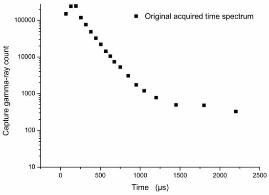
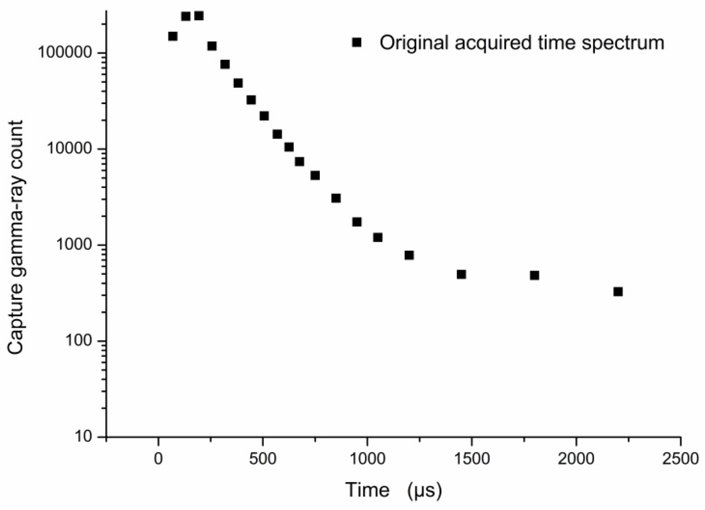
Under given borehole and formation conditions, the capture responses from the borehole and formation are superimposed and recorded by the logging instrument as a complete time spectrum. In this study, the time-spectrum sampling process of the logging tool follows an equal-time-interval sampling scheme. The continuous time domain t ∈ [0, T] in Equation (1), where T denotes the total acquisition time (2400 μs) in this study, is discretized into n time channels. The i − th channel corresponds to the interval [t_i−1,t_i], with a constant channel width of Δt = t_i − t_i−1 (μs). With Δt = 1 (μs), the number of time channels is n = 2400 in this study. Because equal-time-interval sampling is adopted, each time channel uniquely corresponds to a specific time interval; therefore, the boundaries used in the subsequent analysis are expressed in terms of time. After discretization, the time spectrum is represented as a discrete sequence, in which $N_i^{\mathit{acq}}$ denotes the gamma-ray count of the i − th channel. For notational convenience, the count corresponding to time t_i is expressed as $N_i^{\mathit{acq}}=N^{\mathit{acq}}(t_i)$. The original acquisition time spectrum, ${\left\{N_i^{\mathit{acq}}\right\}}_{i=1}^{2400}$, plotted on a logarithmic vertical scale, is shown in Figure 1.

Figure 1. Schematic representation of the original acquired time spectrum. The 2400-channel measured spectrum is simplified to 19 representative points for illustration of the subsequent processing procedure.

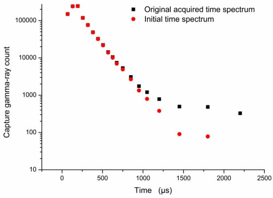
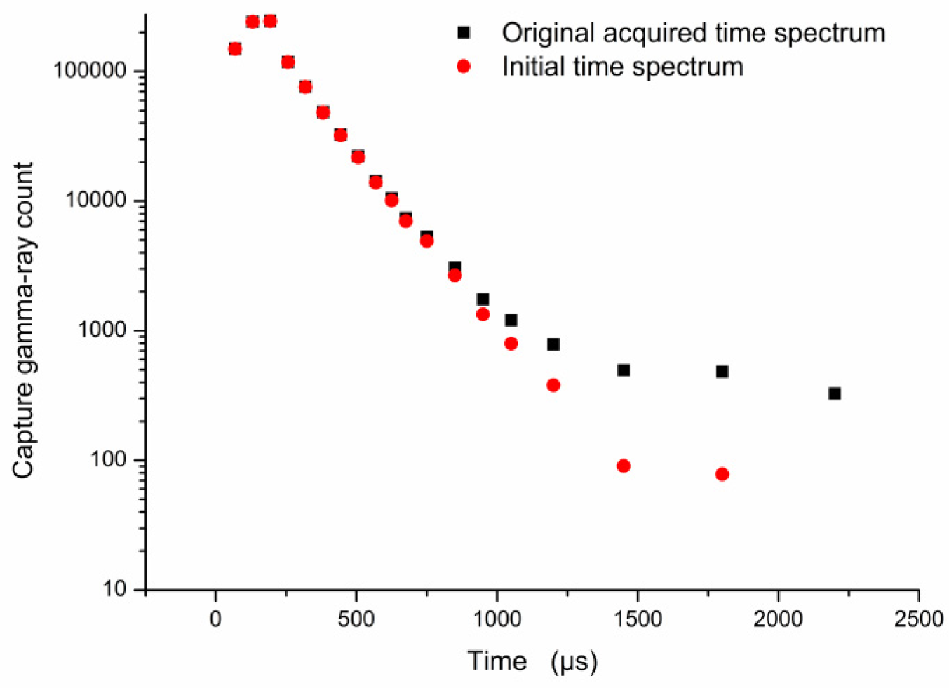
Because the natural gamma-ray background of the formation may interfere with the acquired time spectrum, background subtraction is performed first. In this study, a dynamic background-search method is used to determine the natural gamma-ray background, and the starting channel of the background region is denoted by n_bk. When the gamma-ray count fluctuations in all channels from channel n_bk to channel 2400 fall below the characteristic fluctuation level of the natural gamma-ray background, n_bk is identified as the starting channel of the natural gamma-ray background. Previous studies have shown that thermal neutrons generally decay within approximately 0.5–2 ms after a neutron burst [23], and delayed time gates have been used to estimate background counts in pulsed neutron capture logging [24]. Accordingly, the interval of 1800–2400 μs was selected as the initial background estimation window in this study, where the capture-gamma contribution was assumed to be small. The background estimate was then refined by searching earlier time channels and updating the estimate when the channel count fell below the current background level. The resulting background estimate was used for subsequent time-spectrum correction. In addition, counting-statistical fluctuations may cause local abrupt variations in the acquired time spectrum, potentially leading to erroneous results in subsequent local calculations. Therefore, after subtraction of the natural gamma-ray background, the time spectrum is smoothed to suppress counting-statistical fluctuations. In this study, a five-point Hamming filter is applied to the background-corrected time spectrum, yielding the initial time spectrum.

After natural gamma-ray background subtraction and Hamming filtering, the original acquired time spectrum is processed to obtain the initial time spectrum, which is represented as ${\left\{N_i\right\}}_{i=1}^{n_{\mathit{bk}}-1}$. Figure 2 compares the original acquired time spectrum and the corresponding initial time spectrum after preprocessing.

Figure 2. Schematic comparison of the original acquired time spectrum and the initial time spectrum after preprocessing.

Because the post-pulse intermediate-to-late portion of the time spectrum contains relatively stable information on the formation thermal-neutron decay behavior, the starting and ending times of the initial formation-sensitive interval are defined as $t_s^{f0}$ and $t_{\mathrm{e}}^{f0}$, respectively. This interval $[t_s^{f0},t_e^{f0}]$ is referred to as the initial formation-sensitive interval. The selection of this interval is critical and satisfies the following criteria:

• $t_s^{f0}<t_e^{f0};t_s^{f0},t_{\mathrm{e}}^{f0}\in [t_1,t_{n_{\mathit{bk}}-1}]$;
• $N(t_s^{f0})>0,N(t_e^{f0})>0$;

By substituting Equation (3) into Equation (1) and applying the logarithmic change-of-base formula, the relationship between the capture gamma-ray count and formation sigma is as shown in Equation (5).

$${\Sigma }_f^{(0)}=10466\times {\displaystyle \frac{({\log }_{10}N(t_s^{f0})-{\log }_{10}N(t_e^{f0}))}{t_e^{f0}-t_s^{f0}}}$$

(5)

where $N(t_s^{f0})$ and $N(t_e^{f0})$ denote the capture gamma-ray counts at $t_{\mathrm{s}}^{f0}$ and $t_{\mathrm{e}}^{f0}$, respectively; log₁₀ denotes the base-10 logarithm; and ${\Sigma }_f^{(0)}$ denotes the formation sigma estimated from the initial formation-sensitive interval, with a unit of c.u.

According to Equation (5), ${\Sigma }_f^{(0)}$ is directly proportional to the gamma-ray decay rate within the initial formation-sensitive interval, where the decay rate is characterized by the slope of the logarithmic capture gamma-ray count with respect to time. To reduce the random error associated with the use of individual time points, the logarithms of capture gamma-ray counts within the interval from $t_{\mathrm{s}}^{f0}$ to $t_{\mathrm{e}}^{f0}$ are linearly fitted using the least-squares method. The resulting decay equation is expressed as

log₁₀N(t) = −K^f0 × t + b^f0

(6)

where N(t) denotes the capture gamma-ray count at time t within the initial formation-sensitive interval; K^f0 denotes the gamma-ray decay rate obtained by least-squares fitting, with −K^f0 representing the slope of the fitted line; and b^f0 is the fitted intercept. By combining Equations (5) and (6), the relationship expressed in Equation (7) is obtained.

$${\Sigma }_f^{(0)}=10466\times K^{f0}$$

(7)

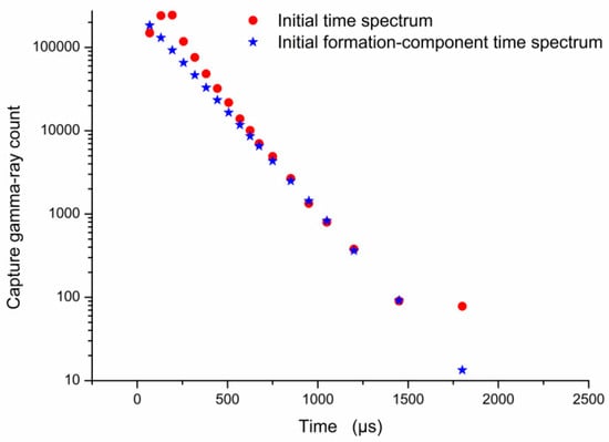
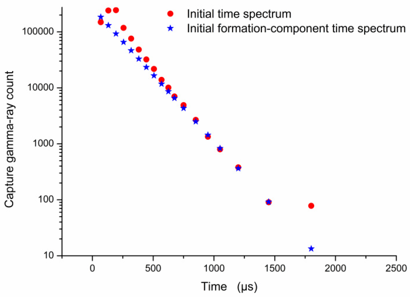
To separate the formation and borehole components, the discrete sampling times t_i are substituted into Equation (6), and the corresponding initial formation-component counts are obtained through inverse logarithmic transformation:

$$N_i^{f0}={10}^{-K^{f0}\times t_i+b^{f0}},i=1,2,\dots ,n_{\mathit{bk}}-1$$

(8)

Based on the fitting result of the initial formation-sensitive interval, a discrete array representing the initial formation-component time spectrum, ${\left\{N_i^{f0}\right\}}_{i=1}^{n_{\mathit{bk}}-1}$, is then constructed. A schematic illustration is shown in Figure 3.

Figure 3. Schematic illustration of the initial time spectrum and the reconstructed initial formation-component time spectrum.

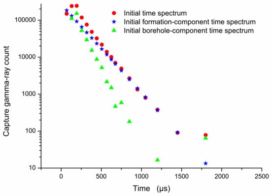
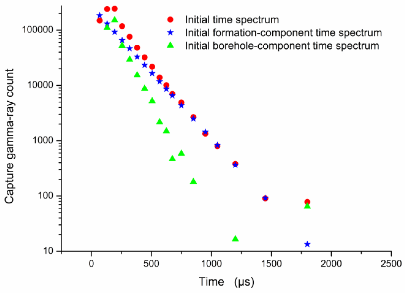
The initially separated borehole-component time spectrum ${\left\{N_i^{b0}\right\}}_{i=1}^{n_{\mathit{bk}}-1}$ is obtained by subtracting the initial formation-component time spectrum ${\left\{N_i^{f0}\right\}}_{i=1}^{n_{\mathit{bk}}-1}$ from the initial time spectrum ${\left\{N_i\right\}}_{i=1}^{n_{\mathit{bk}}-1}$ channel by channel, as expressed in Equation (9):

$$N_i^{b0}=N_i-N_i^{f0}, i=1,2,\dots ,n_{\mathit{bk}}-1$$

(9)

A schematic illustration is shown in Figure 4.

Figure 4. Schematic illustration of the initial time spectrum and the initially separated formation and borehole components.

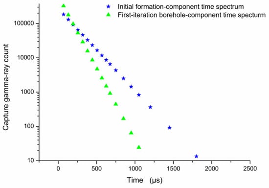
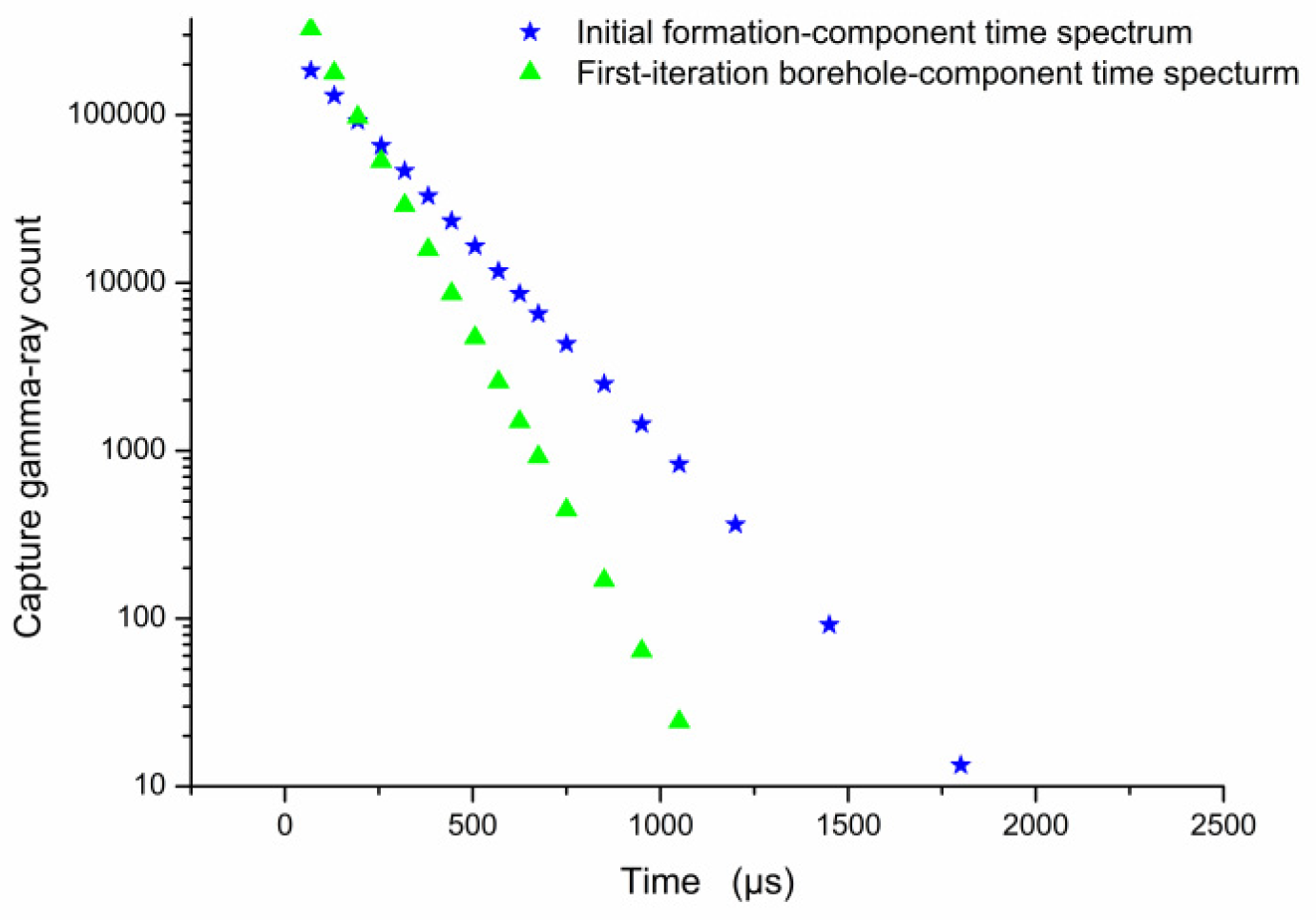
The initially separated borehole-component time spectrum still contains a certain contribution from the formation component. Therefore, an early-time interval of the initially separated borehole-component time spectrum is selected and fitted using the least-squares method to obtain the corresponding borehole decay model. Based on this fitting result, the borehole-component time spectrum after the first iteration is reconstructed, as schematically illustrated in Figure 5.

Figure 5. Schematic illustration of the initial formation-component time spectrum and the borehole-component time spectrum reconstructed after the first iteration.

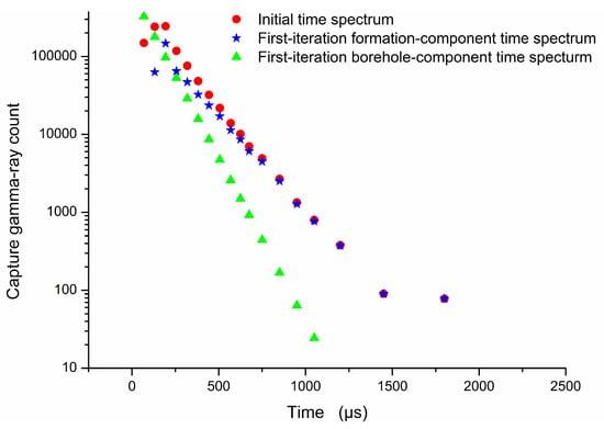
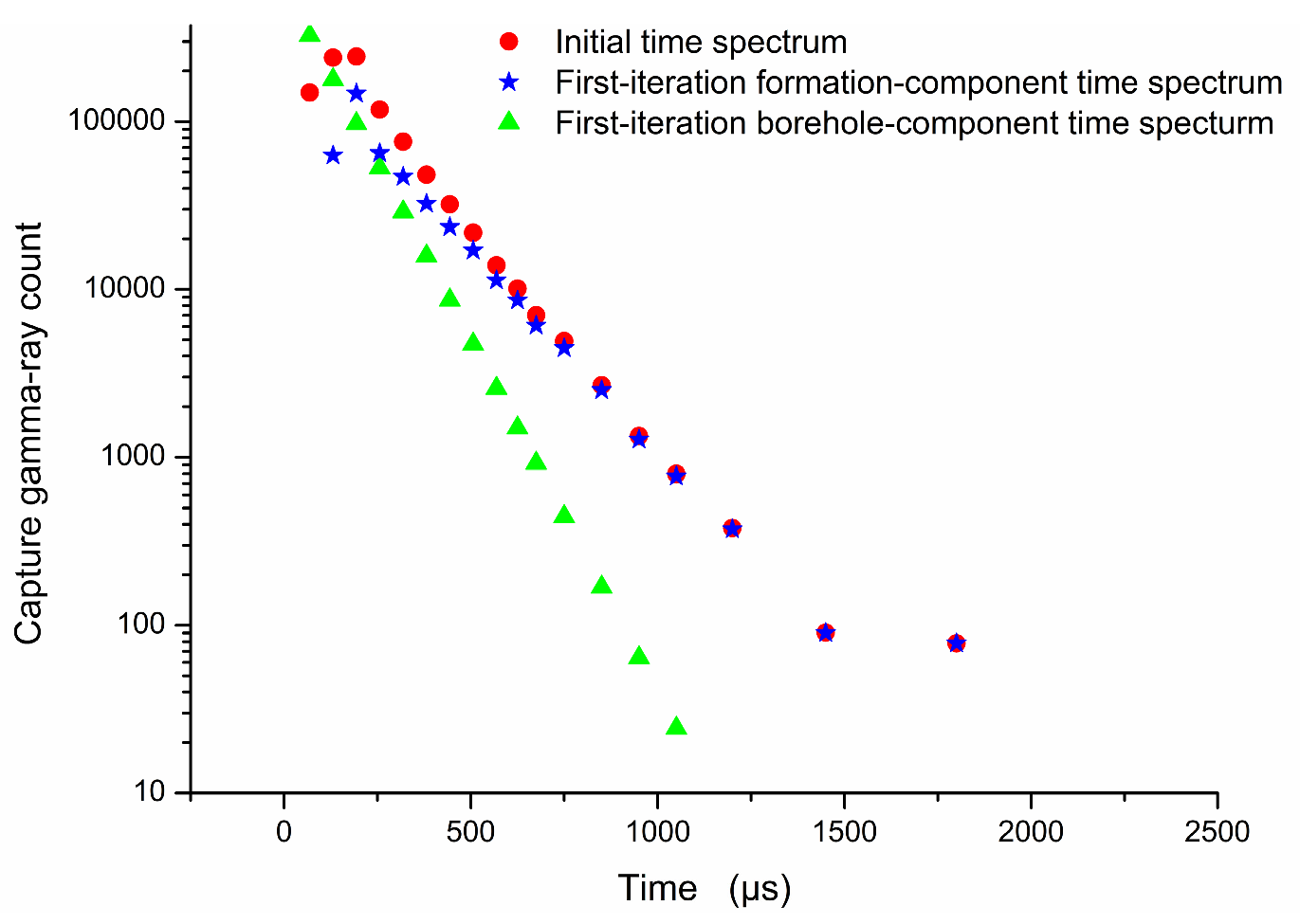
The first-iteration formation-component time spectrum is obtained by subtracting the first-iteration borehole-component time spectrum from the initial time spectrum. This step completes the first iteration of the borehole–formation component separation process, as schematically illustrated in Figure 6.

Figure 6. Schematic illustration of the initial time spectrum and the borehole and formation components obtained after the first iteration.

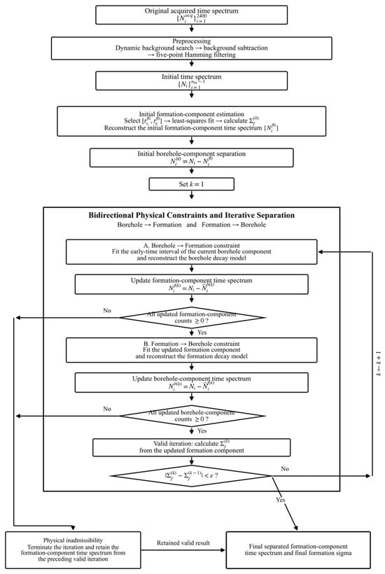
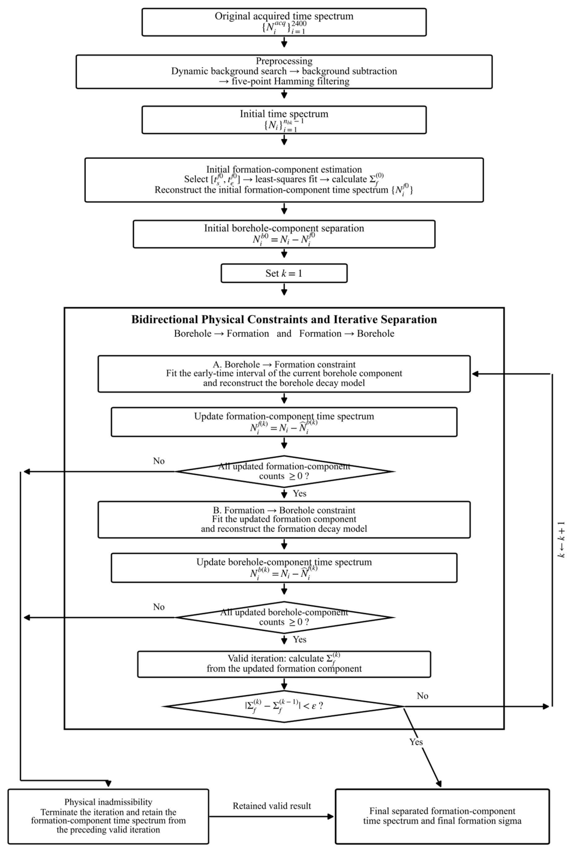
The above procedure is repeated iteratively to progressively refine the separation of the borehole and formation components. During each iteration, the fitted borehole component is used to update the formation component, while the fitted formation component is subsequently used to update the borehole component. Since the borehole and formation components represent gamma-ray count contributions, both must satisfy the non-negativity requirement. If either updated component contains a negative count within the formation-sensitive interval, the current iteration is considered physically inadmissible and is terminated. The formation-component spectrum from the preceding valid iteration is then retained for apparent-Sigma estimation. This non-negativity requirement serves as a physical admissibility constraint during component separation rather than a complete description of neutron transport. In addition, after each valid iteration, the formation sigma, denoted by ${\Sigma }_f^{(k)}$, is calculated from the updated formation-component time spectrum. Because formation sigma is the target parameter of PNL interpretation, its variation between two consecutive iterations is used as the convergence criterion. When

$$|{\Sigma }_f^{(k)}-{\Sigma }_f^{(k-1)}|<\epsilon$$

(10)

the iterative process is considered converged and is terminated, where ε is the prescribed convergence threshold. In this study, ε was set to 1 × 10⁻³ c.u.

A flowchart of the proposed time-spectrum processing algorithm based on borehole–formation separation and bidirectional constraints is shown in Figure 7.

Figure 7. Flowchart of the proposed time-spectrum processing algorithm based on borehole–formation separation and bidirectional constraints.

3. Monte Carlo-Based Simulation Study

In this study, Monte Carlo numerical simulations were performed to obtain capture gamma-ray time-spectrum data from neutron lifetime logging in cased wells and to validate the proposed method. Monte Carlo simulation offers distinct advantages for evaluating new methods in pulsed neutron lifetime logging, as it enables idealized logging responses to be simulated using predefined formation parameters. By comparing the results obtained with the proposed method against the known formation parameters, the feasibility and effectiveness of the method can be readily assessed [17].

3.1. Simulation Model Parameters

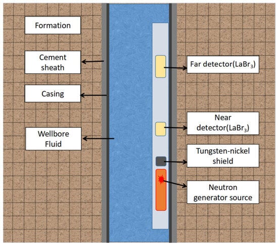
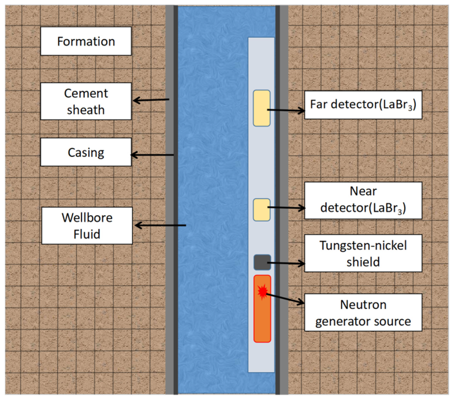
To investigate the distribution characteristics of the capture gamma-ray time spectrum, a basic Monte Carlo numerical simulation model was established, as shown in Figure 8. The capture gamma-ray time-spectrum distributions under different environmental conditions were simulated using this model.

Figure 8. Basic Monte Carlo numerical simulation model.

The basic cased-well formation model consists of a borehole section containing water, casing, and cement sheath. The borehole diameter is set to 8.5 in. (215.9 mm), and a 7 in. casing is used, with inner and outer diameters of 157.08 mm and 177.80 mm, respectively. The cement sheath thickness is set to 19.05 mm, which corresponds to typical parameters of an 8.5 in. cased well. In the numerical simulation, a formation model with a radial thickness of 70 cm and a height of 150 cm was established. The formation model was discretized into grid cells with a radial spacing and vertical height of 5 cm, and different lithologies and fluids were assigned to the corresponding cells.

A D-T pulsed neutron generator was used as the neutron source, with a neutron yield of 10⁸ cps. The neutron pulse width was set to 200 μs during the simulation. Gamma photons were detected using two LaBr3 scintillation detectors, with near and far detector source distances of 35 cm and 58 cm, respectively. The recording time window of the gamma-ray detectors for thermal neutron capture information was set from 0 to 2400 μs with a time interval of 1 μs. Based on the above simulation parameters, the capture gamma-ray time-spectrum data were obtained.

3.2. Validation of Algorithm Feasibility

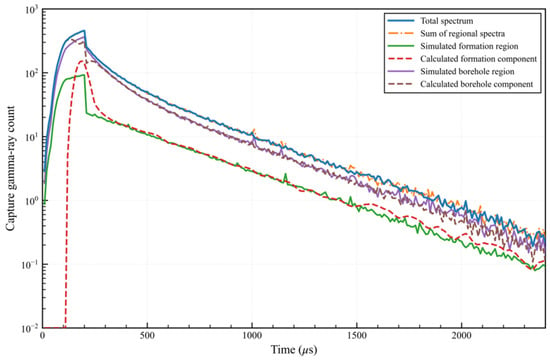
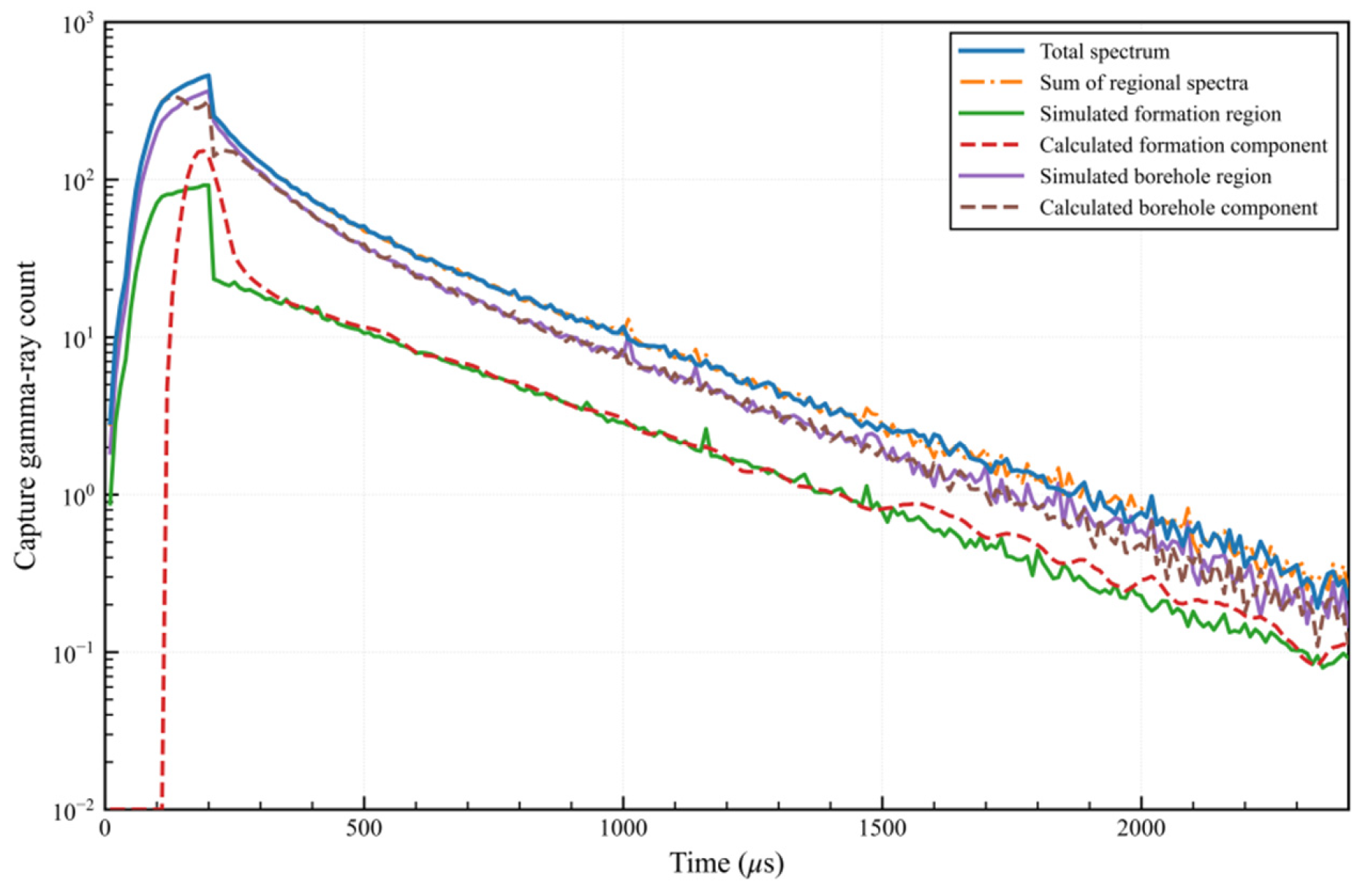
Based on the basic model shown in Figure 8, the formation was set as sandstone with a porosity of 20%, fully saturated with 20,000 ppm saline water, and the borehole fluid was set as fresh water. The total time spectrum was obtained from all detected capture gamma rays. To distinguish the formation- and borehole-origin contributions, separate Monte Carlo simulations were performed by selectively enabling neutron-induced gamma-ray production in the corresponding regions, with the borehole region including the wellbore fluid, casing, and cement sheath. Neutron and gamma-ray transport, including scattering and attenuation, were retained in these simulations. Thus, the resulting component spectra represent detector responses associated with different gamma-ray production regions rather than gamma rays counted directly at their production locations. Coupled neutron–gamma transport simulations have previously been applied and benchmarked in nuclear well logging [25]. The near-detector spectra are shown in Figure 9.

Figure 9. Comparison of the Monte Carlo-simulated total, formation-region, and borehole-region time spectra with the formation and borehole components obtained using the proposed method for the near detector.

The simulated total time spectrum agrees well with the sum of the simulated formation-region and borehole-region time spectra, indicating that the regional contributions obtained through separate Monte Carlo simulations with region-selective gamma-ray production are consistent with the total detector response. These simulated regional spectra were then used as references to evaluate the proposed method. The calculated formation-component and borehole-component time spectra agree well with the corresponding simulated regional spectra, demonstrating the effectiveness of the proposed separation method.

The natural gamma-ray background was not included in the Monte Carlo model. The simulated total, borehole-region, and formation-region time spectra decrease to below 1 count at approximately 1800, 1700, and 1500 μs, respectively, indicating that the contribution of capture gamma rays becomes negligible at late times. Therefore, for practical measurements, gamma-ray counts recorded after approximately 1600 μs can be reasonably regarded as being dominated by the natural gamma-ray background, providing a basis for dynamically determining the background interval.

A comparison between the calculated formation-component time spectrum and the simulated formation-region time spectrum shows a certain deviation within the interval of 200–400 μs. To quantify the residual mismatch observed in Figure 9, the reconstructed formation-component spectrum was compared with the simulated formation-region spectrum over 200–400 μs. The normalized mean absolute residual was 61.47%. Notably, 96% of the total absolute residual was concentrated within 200–235 μs, indicating that the discrepancy was predominantly confined to the earliest part of the examined interval. This behavior is consistent with the stronger influence of borehole contributions at early times. Since formation apparent-Sigma estimation is performed over the later formation-sensitive interval of 600–1300 μs, the early-time discrepancy is excluded from the direct fitting procedure.

The calculated formation-component time spectrum and the simulated formation-region time spectrum exhibit highly consistent profiles from 400 to 1400 μs, and the minimum count values remain above 1 throughout this interval. These results demonstrate that the proposed time-spectrum processing method can effectively separate the formation-component and borehole-component time spectra. Nevertheless, during the initial stage (200–400 μs), where the borehole contribution dominates, the influence of the borehole region cannot be completely eliminated. This deviation does not affect formation sigma estimation because the early interval with strong borehole interference is excluded from subsequent fitting. For the subsequent calculation of sigma, the initial stage with significant borehole interference should be excluded, and the tail region of the time spectrum with considerable statistical fluctuations should also be avoided. Consequently, a more accurate sigma can be obtained.

The simulated and calculated borehole-region time spectra exhibit two distinct decay stages, approximately 200–400 μs and 400–1400 μs. This behavior is associated with the complex neutron transport and capture processes in the heterogeneous borehole environment [9,26].

3.3. Analysis of Time-Spectrum Characteristics

The decay characteristics of the time spectrum are affected by borehole size, borehole fluid properties, formation lithology, porosity, and formation fluid properties. Based on the simulation method described above, time spectra under different borehole, lithological, and porosity conditions were obtained and analyzed to provide guidance for formation sigma estimation. The near-detector time spectrum was selected as an example to investigate the characteristics of the formation-region time spectrum.

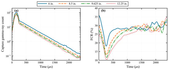
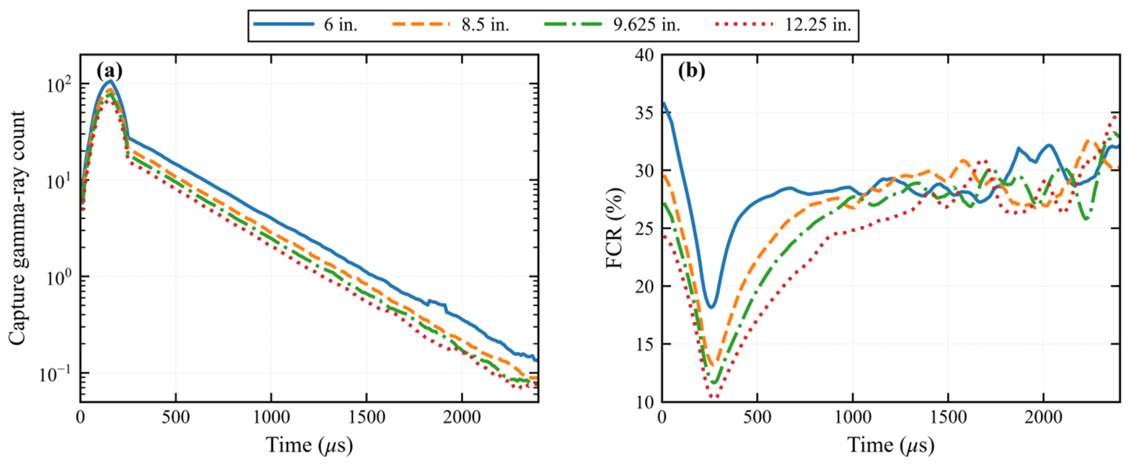
Based on the basic model shown in Figure 8, four borehole sizes (6 in., 8.5 in., 9.625 in., and 12.25 in.) were considered. The casing and cement sheath geometries were adjusted accordingly, while their thicknesses were kept unchanged. The borehole fluid salinity was set to 0 ppm. The formation was modeled as sandstone with a porosity of 20%, fully saturated with 20,000 ppm brine. Monte Carlo simulations were used to obtain the total, formation-region, and borehole-region time spectra. The formation-region contribution ratio (FCR) was calculated as the ratio of the formation-region count to the corresponding total count at each time channel, as defined in Equation (11).

$$C_i^f={\displaystyle \frac{N_i^f}{N_i}}\times 100, i=1,2,\dots 2400,N_i>0$$

(11)

where ${\mathrm{N}}_i^f$ and N_i denote the capture gamma-ray counts of the formation-region and total time spectra at time channel i, respectively. $C_i^f$ is the formation-region contribution ratio (FCR), expressed as a percentage (%).

Figure 10 presents the formation-region time spectra and corresponding FCRs for different borehole sizes. After the neutron pulse ends, the formation-region time spectra quickly enter a stable decay regime. In this regime, the spectra for different borehole sizes exhibit nearly parallel decay trends, indicating that variations in borehole size mainly affect the absolute count intensity but have little influence on the decay rate. The FCR decreases with increasing borehole size and becomes relatively stable after approximately 600 μs. At late times, the fluctuations increase because of counting-statistical fluctuations. Overall, the FCR remains below 35%.

Figure 10. Formation-region time spectra (a) and corresponding FCRs (b) for different borehole sizes.

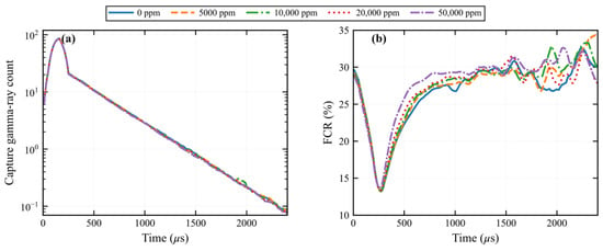
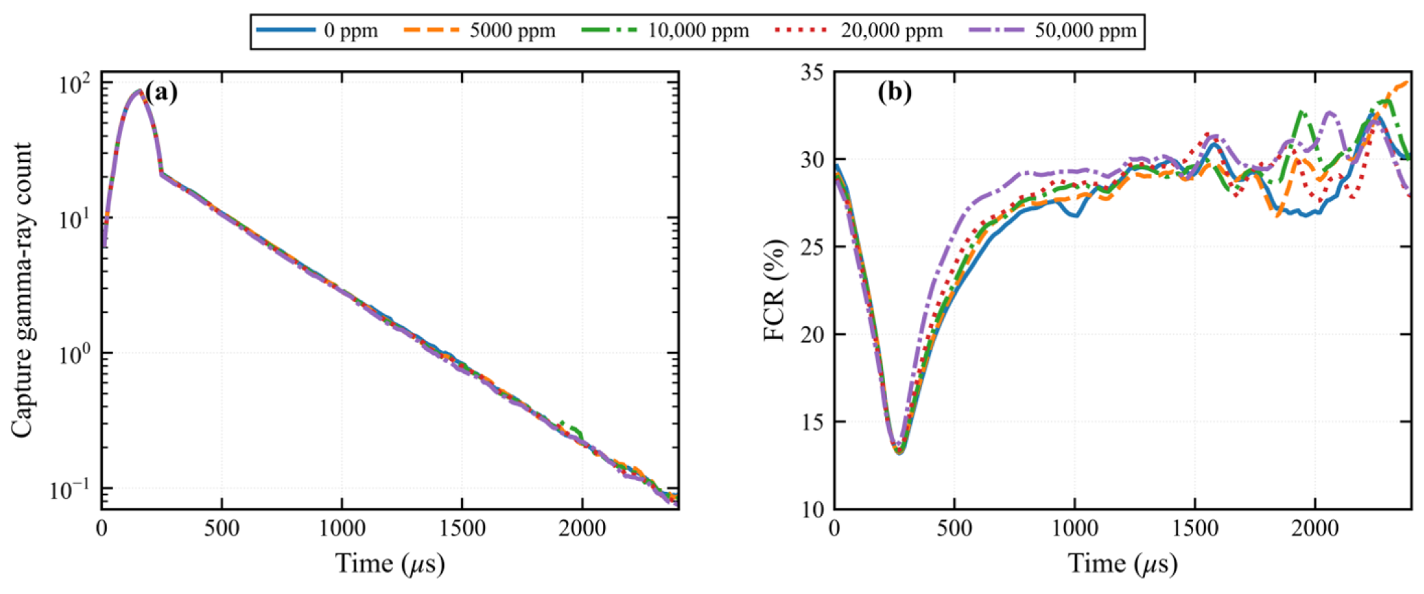
Under the basic model conditions, the borehole fluid salinities were set to 0, 5000, 10,000, 20,000, and 50,000 ppm. The formation was modeled as sandstone with a porosity of 20%, fully saturated with 20,000 ppm brine. Monte Carlo simulations were used to obtain the total, formation-region, and borehole-region time spectra. The formation-region time spectra and corresponding FCRs are shown in Figure 11.

Figure 11. Formation-region time spectra (a) and corresponding FCRs (b) for different borehole fluid salinities.

As the borehole fluid salinity increases, the formation-region time spectra exhibit nearly complete overlap, indicating that borehole fluid salinity has little influence on the formation-region count intensity or decay characteristics under the modeled conditions. In contrast, the FCR shows a modest dependence on borehole fluid salinity. After approximately 600 μs, higher borehole fluid salinity generally results in a slightly higher FCR, which is consistent with the faster decay of the borehole contribution caused by enhanced thermal-neutron capture in saline borehole fluid. Within the effective analysis interval up to 1500 μs, the FCR remains below 30%.

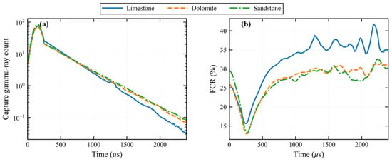
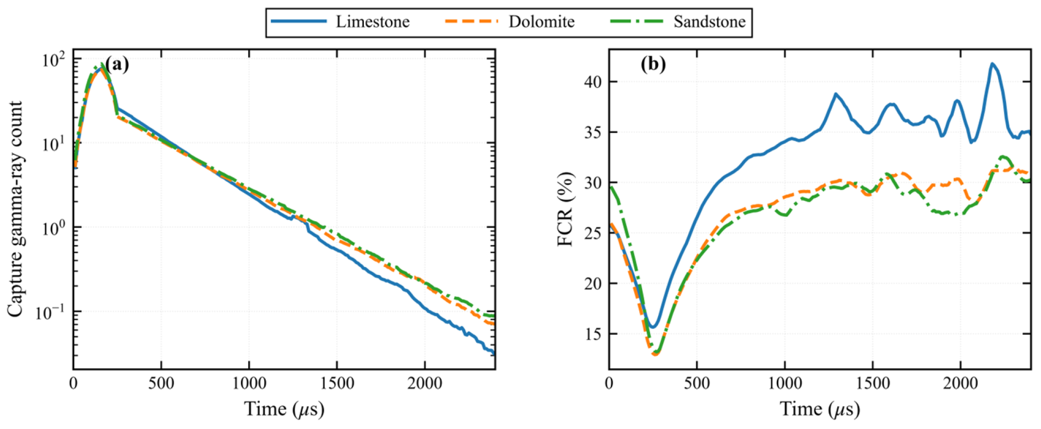
Based on the basic model, the borehole fluid salinity was set to 0 ppm, and the formation lithology was varied among sandstone, limestone, and dolomite. The formation porosity was fixed at 20%, with the pore space fully saturated by 20,000 ppm brine. Monte Carlo simulations were used to obtain the total, formation-region, and borehole-region time spectra. The formation-region time spectra and corresponding FCRs are shown in Figure 12.

Figure 12. Formation-region time spectra (a) and corresponding FCRs (b) for different lithologies.

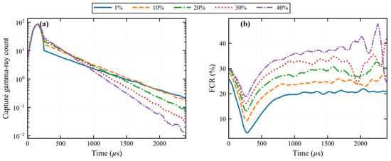
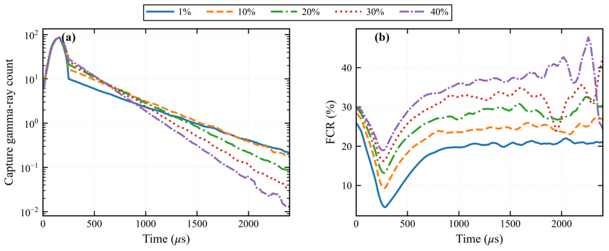
Based on the basic model, the borehole fluid salinity was set to 0 ppm, and the formation was modeled as sandstone with a formation-water salinity of 20,000 ppm. Formation porosities of 1%, 10%, 20%, 30%, and 40% were investigated, with the pore space fully saturated with formation water. Monte Carlo simulations were used to obtain the total, formation-region, and borehole-region time spectra. The formation-region time spectra and corresponding FCRs are shown in Figure 13.

Figure 13. Formation-region time spectra (a) and corresponding FCRs (b) for different formation porosities.

With increasing formation porosity, the formation-region time spectrum decays faster. After the neutron pulse ends at 200 μs, the spectra enter a stable decay regime, while the FCR increases and becomes relatively stable after approximately 600 μs; higher porosity generally yields a higher FCR. Within the effective analysis interval, the FCR remains below 40%, whereas late-time fluctuations caused by low counts are excluded from formation sigma estimation.

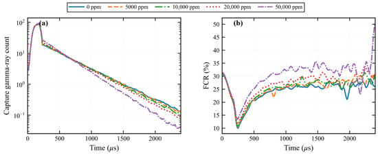
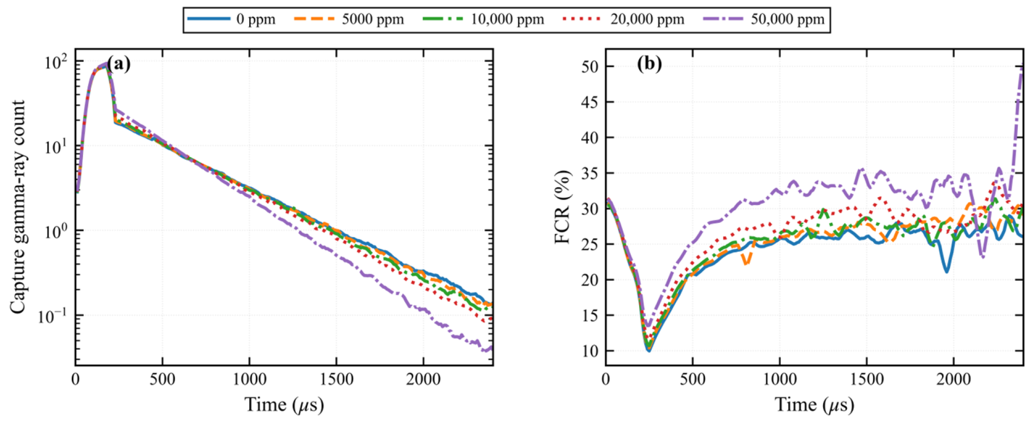
Based on the basic model, the borehole fluid salinity was fixed at 0 ppm, and a sandstone formation with 20% porosity was modeled with formation-water salinities of 0, 5000, 10,000, 20,000, and 50,000 ppm. The pore space was fully saturated with formation water. Monte Carlo simulations were used to obtain the total, formation-region, and borehole-region time spectra. The formation-region time spectra and corresponding FCRs are shown in Figure 14.

Figure 14. Formation-region time spectra (a) and corresponding FCRs (b) for different formation-water salinities.

With increasing formation-water salinity, the formation-region time spectrum decays faster, consistent with the expected increase in neutron capture. After neutron pulse termination, the spectra gradually enter a stable decay regime. The FCR generally increases with formation-water salinity and becomes relatively stable after approximately 600 μs. Within the effective analysis interval, the FCR remains below 35%, while late-time fluctuations are mainly caused by low-count statistics.

Based on the above analyses of the near-detector time spectra and similar results obtained for the far detector, the following conclusions can be drawn to guide the selection and adjustment of key time intervals in the proposed algorithm:

(1)

Borehole and formation conditions affect the formation-region time spectrum in different ways. Increasing borehole size mainly reduces the formation-region count intensity and FCR, with little effect on the decay rate, while borehole fluid salinity has only a minor influence on the formation-region spectrum. In contrast, formation lithology, porosity, and formation-water salinity have more pronounced effects on the decay characteristics. Despite these variations, the formation-region contribution generally remains below approximately 40% within the effective analysis interval, indicating that borehole interference cannot be neglected.

(2)

Formation-region counts become very low after approximately 1500 μs, with increasingly pronounced late-time statistical fluctuations. Combined with the late-time analysis in Section 3.2, approximately 1600 μs can therefore be used as a reference starting point for dynamically determining the natural gamma-ray background interval.

(3)

After neutron pulse termination, the FCR generally becomes relatively stable after approximately 600 μs. Considering both FCR stability and counting statistics, 600–1300 μs provides a suitable reference formation-sensitive interval for initializing formation-component fitting and estimating formation sigma. This reference interval can be directly used for the iterative processing under the investigated conditions.

(4)

For rapidly decaying conditions, such as limestone or high formation-water salinity, the fitting cutoff time may optionally be advanced to reduce the influence of late-time statistical fluctuations and accelerate convergence, although this adjustment is not required for the implementation of the proposed method.

4. Validation and Application of the Proposed Method

4.1. Simulation Validation

To evaluate the feasibility and accuracy of the proposed method under conditions representative of field logging, five validation models were established by modifying the basic model according to the configurations listed in Table 1. Monte Carlo simulations were performed to obtain the total and formation-region time spectra for each case.

Table 1. Modeling parameters of the five validation models.

Model ID	Borehole Diameter (in.)	Lithology	Borehole Fluid Salinity (ppm)	Formation Water Salinity (ppm)	Porosity (%)	Oil Saturation (%)
M1	8.5	Limestone	10,000	10,000	20	100
M2	8.5	Sandstone	5000	10,000	30	50
M3	12.25	Dolomite	0	30,000	25	30
M4	12.25	Limestone	20,000	0	35	80
M5	12.25	Sandstone	30,000	30,000	15	20

The five validation models were constructed separately from those used for the parameter analysis in Section 3. The formation-sensitive interval and other algorithm parameters were determined during method development and kept unchanged throughout the validation. The same iterative procedure was applied to all five models, while the number of iterations was determined by the stopping criteria. The reference apparent-Sigma values were used only for error evaluation and were not involved in parameter selection or iterative separation.

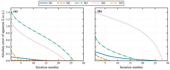
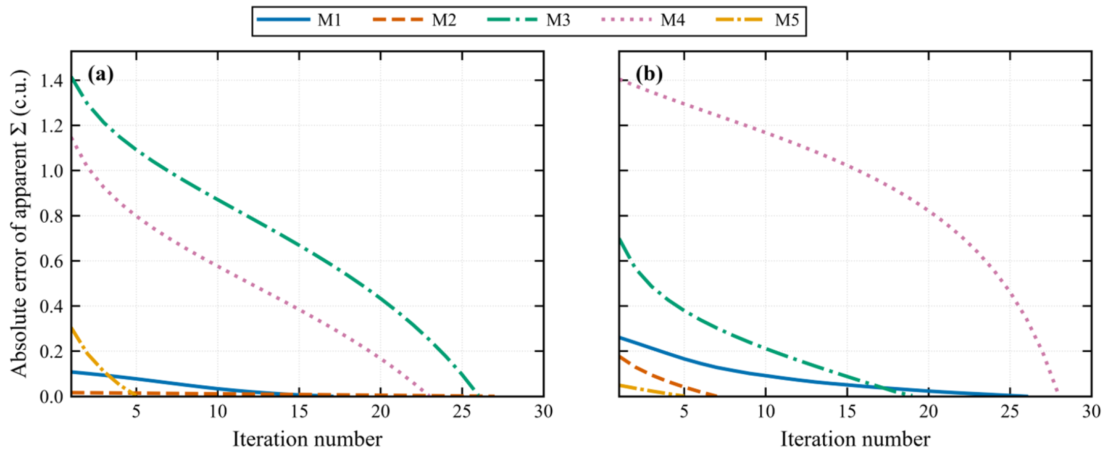
Because the measured time-spectrum decay is affected by neutron diffusion, the sigma derived directly from the time spectrum is referred to as apparent Sigma(Σapp) [5]. The single-exponential fitting procedure is used to estimate this apparent Sigma rather than to describe the complete neutron-transport process. For each detector, the apparent Sigma obtained from the simulated formation-region time spectrum was defined as the theoretical apparent Sigma and used as the reference value for validation. The proposed method was then applied to the total time spectrum, and the apparent Sigma obtained from the separated formation-component time spectrum after each iteration was defined as the calculated apparent Sigma. The absolute difference between the calculated and theoretical apparent Sigma was defined as the iteration error. The iteration error curves of the five validation models are presented in Figure 15.

Figure 15. Iteration-error curves of apparent Sigma estimation for the near (a) and far (b) detectors.

As shown in Figure 15, the number of iterations required for convergence varies among the five field-relevant validation models. Nevertheless, the iteration errors decrease progressively to near zero for all models, demonstrating stable iteration and reliable convergence of the proposed method under representative logging conditions.

The termination behavior of the proposed algorithm was further examined using the five validation models, as summarized in Table 2. Among the ten calculations for the near and far detectors, six (60%) satisfied the Sigma convergence criterion, while four (40%) were terminated by the non-negativity constraint. In all four cases, the first negative count was detected in the formation component between 1273 and 1286 μs, near the end of the formation-sensitive interval (600–1300 μs). No termination was triggered by the borehole component. When the non-negativity constraint was triggered, the preceding valid iteration was retained for formation apparent-Sigma estimation.

Table 2. Termination behavior of the proposed algorithm for the five validation models.

Model ID	Near Detector	Far Detector
M1	Sigma convergence	Sigma convergence
M2	Sigma convergence	Sigma convergence
M3	Non-negativity (1285 μs)	Sigma convergence
M4	Sigma convergence	Non-negativity (1286 μs)
M5	Non-negativity (1273 μs)	Non-negativity (1286 μs)

Note: The values in parentheses indicate the time channels at which negative counts were first detected in the formation component.

4.2. Sensitivity Analysis of the Initial Formation-Sensitive Interval

To evaluate the influence of the initial formation-sensitive interval on the final formation sigma, a sensitivity analysis was performed using the five validation models (M1–M5) described in Table 1. The interval of 600–1300 μs, determined from the time-spectrum characteristics discussed in Section 3.3, was used as the reference. To isolate the influence of the initial interval position from that of the interval width, the starting and ending times were shifted simultaneously while maintaining a constant interval width of 700 μs. The interval was shifted from −200 to +200 μs in increments of 20 μs, resulting in 21 different interval positions. All other processing parameters remained unchanged. For each shifted interval, the apparent Sigma values obtained from the near and far detectors were subjected to the same multi-detector correction procedure described in Section 4.3 to account for borehole and neutron-diffusion effects. The correction procedure and instrument-specific calibration parameters were kept identical for all interval settings.

The variation in the final formation Sigma was calculated relative to the result obtained using the original interval of 600–1300 μs:

$$\Delta \Sigma \_f(\delta )=\Sigma \_f(0)-\Sigma \_f(\delta )$$

(12)

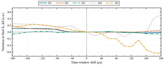
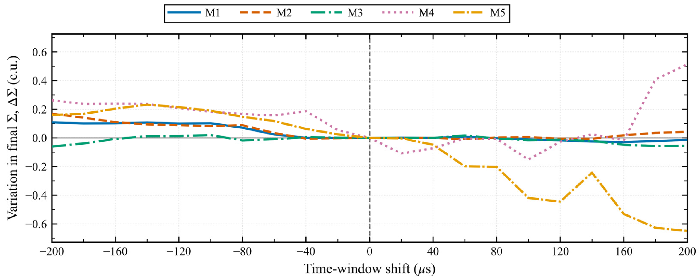
where δ denotes the time-window shift, $\Delta \Sigma \_f(\delta )$ is the variation in final formation Σ (c.u.), and $\Sigma \_f(0)$ and $\Sigma \_f(\delta )$ represent the final formation sigma obtained using the original and shifted intervals, respectively. The corresponding results are presented in Figure 16.

Figure 16. Variation in the final formation sigma with shifts in the initial formation-sensitive interval for the five validation models.

Figure 16 shows the variations in the final formation Sigma for the five validation models. When the initial interval is shifted within ±100 μs, the maximum absolute Sigma variation among the five models is 0.419 c.u. Extending the shift range to ±140 μs results in a maximum absolute variation of 0.445 c.u. For shifts toward earlier times of up to 200 μs, the maximum absolute variation remains below 0.263 c.u.

Over the full shift range of ±200 μs, the maximum absolute variations for M1, M2, and M3 are 0.108, 0.169, and 0.061 c.u., respectively. However, M4 and M5 exhibit greater sensitivity when the interval is shifted toward later times. At a shift of +200 μs, their absolute Sigma variations reach 0.513 and 0.649 c.u., respectively. This increased sensitivity may be associated with lower count levels and greater relative statistical fluctuations in the late-time spectrum.

These results indicate that the final formation Sigma remains relatively stable when the initial formation-sensitive interval is adjusted within a reasonable range. The interval of 600–1300 μs therefore provides a suitable reference for initializing the iterative separation process under the investigated conditions. However, excessive shifts toward later times may lead to increased variations in the final Sigma estimates for certain borehole and formation conditions.

4.3. Error Analysis and Accuracy Evaluation

Using the reference apparent Sigma values directly calculated from the Monte Carlo formation-region time spectra in Section 4.1, the apparent-Sigma estimation accuracies of the near and far detectors were evaluated for the proposed method and double-exponential fitting. For a consistent comparison, double-exponential fitting was applied to the same preprocessed time spectra using fixed settings for all validation models, without model-specific tuning. The results are summarized in Table 3.

Table 3. Comparison of reference and calculated apparent Sigma values for the near and far detectors.

Detector	Model ID	Reference Σapp (c.u.)	Calculated Σapp (c.u.)		Relative Error (%)
			Dual-exp.	Proposed	Dual-exp.	Proposed
Near Detector	M1	13.3533	13.5587	13.3533	1.5382	0.0000
	M2	13.0590	13.2331	13.0589	1.3332	0.0007
	M3	13.8783	14.0515	13.8829	1.2478	0.0331
	M4	15.8852	15.1515	15.8843	4.6188	0.0057
	M5	11.6321	12.5859	11.6291	8.1997	0.0258
Far Detector	M1	11.1510	12.1733	11.1511	9.1678	0.0009
	M2	11.2970	11.9236	11.2969	5.5466	0.0009
	M3	12.3923	12.3528	12.3891	0.3187	0.0258
	M4	14.1180	14.9984	14.1202	6.2360	0.0156
	M5	9.7925	10.9357	9.7931	11.6742	0.0061

As shown in Table 3, the proposed method substantially improves the accuracy of apparent Sigma estimation for both the near and far detectors. For the near detector, the relative errors of double-exponential fitting range from 1.25% to 8.20%, whereas those of the proposed method remain below 0.034%. For the far detector, the corresponding errors are 0.32–11.67% and below 0.026%, respectively. These results demonstrate that the proposed borehole–formation separation effectively suppresses borehole contamination in the measured time spectrum and enables the separated formation component to more closely represent the formation response, thereby significantly improving apparent Sigma estimation accuracy under field-relevant conditions.

To further evaluate the performance of the conventional double-exponential fitting method, model-specific optimization was performed for the five validation models. Unlike the original implementation with a fixed fitting start time, the fitting windows were individually adjusted using the reference apparent-Sigma values as optimization targets. The results are presented in Table 4.

Table 4. Apparent-Sigma estimates obtained using the optimized double-exponential fitting method.

Detector	Model ID	Reference Σapp (c.u.)	Calculated Σapp (c.u.)	Relative Error (%)
Near Detector	M1	13.3533	13.3569	0.027
	M2	13.0590	13.1438	0.649
	M3	13.8783	13.9247	0.334
	M4	15.8852	15.5397	2.175
	M5	11.6321	12.1334	4.310
Far Detector	M1	11.1510	11.3426	1.7180
	M2	11.2970	11.3542	0.5060
	M3	12.3923	12.3324	0.4830
	M4	14.1180	14.3560	1.6860
	M5	9.7925	10.2316	4.4840

The optimized double-exponential fitting method achieved improved apparent-Sigma estimates compared with the original fixed-window implementation. The mean relative errors were 1.499% and 1.776% for the near and far detectors, respectively, with an overall mean of 1.637%. Nevertheless, the maximum relative errors remained 4.310% for the near detector and 4.484% for the far detector. These residual deviations suggest that parameter optimization alone cannot fully eliminate the influence of borehole contributions and other factors affecting the mixed decay spectrum.

Furthermore, the improved results were obtained through model-specific optimization guided by known reference apparent-Sigma values, which are generally unavailable in actual logging applications. Therefore, achieving comparable optimization for varying downhole conditions would be challenging [17,27]. In contrast, the proposed method does not require reference-guided parameter adjustment for individual models and maintains higher apparent-Sigma estimation accuracy across the validation cases.

The theoretical formation sigma of each validation model can be calculated using the volumetric mixing model, as given in Equation (13).

$$\Sigma =(1-\phi )\times {\Sigma }_{\mathit{ma}}+\phi \times [(1-S_o)\times {\Sigma }_w+S_o\times {\Sigma }_o]$$

(13)

where $\Sigma$ is the theoretical formation sigma (c.u.); φ is the formation porosity as a fraction; s_o is the oil saturation as a fraction; and ${\Sigma }_{\mathit{ma}}$, ${\Sigma }_w$, and ${\Sigma }_o$ are the macroscopic capture cross sections of the formation matrix, formation water, and oil, respectively (all in c.u.).

The theoretical macroscopic capture cross sections of the formation matrix and formation fluids used in the validation models are listed in Table 5.

Table 5. Theoretical macroscopic capture cross sections of materials used in the validation models.

Material	Density (g/cm3)	Macroscopic Capture Cross Section (c.u.)
Quartz (SiO2)	2.65	4.5530
Calcite (CaCo3)	2.71	7.0800
Dolomite [CaMg(Co3)2]	2.87	4.6971
Fresh water (H2O)	1.00	22.2426
Oil (C22H46)	0.85	25.3405

For saline formation water, ${\Sigma }_w$ was calculated from the corresponding formation-water salinity as follows:

$${\Sigma }_w=(0.9982+0.716\times {10}^{-6}\times C_w)\times (22.2426+0.3284\times {10}^{-3}\times C_w)$$

(14)

where C_w is the formation-water salinity in ppm and ${\Sigma }_w$ is expressed in c.u. The first parenthetical term accounts for the salinity-dependent brine density.

The theoretical formation-sigma values of the five validation models were calculated using Equations (13) and (14) and used as reference values. The single-exponential fitting procedure provides an estimate of the formation apparent Sigma rather than the intrinsic formation Sigma. Since neutron diffusion is not explicitly considered during fitting, its influence may still be present in the estimated apparent Sigma. The near- and far-detector apparent Sigma values obtained by each time-spectrum processing method were subsequently combined using a multi-detector correction approach for borehole and neutron-diffusion effects, following the general methodology reported by Gilchrist and Trcka [26]. The same correction procedure and instrument-specific calibration parameters were applied to both the double-exponential and proposed methods to ensure a consistent comparison. This correction step is independent of the proposed time-spectrum separation algorithm and is used only as a common downstream processing step. Although this correction reduces the influence of neutron diffusion, some residual diffusion-related bias may remain in the corrected formation Sigma. The resulting formation-sigma estimates are compared in Table 6.

Table 6. Comparison of diffusion-corrected formation sigma values and relative errors for the five validation models.

Model ID	Reference Σ (c.u.)	Diffusion-Corrected Σ (c.u.)		Relative Error (%)
		Dual-exp.	Proposed	Dual-exp.	Proposed
M1	10.7304	10.7743	10.6956	0.4091	0.3244
M2	10.8376	10.6082	10.7991	2.1167	0.3552
M3	11.1443	11.3634	11.1447	1.9665	0.0035
M4	13.2530	12.2831	13.3608	7.3180	0.8137
M5	8.5572	9.7669	8.7629	14.1367	2.4042

As shown in Table 6, after applying the same multi-detector correction procedure, the proposed method provides more accurate formation-sigma estimates than double-exponential fitting for all five validation models. The mean relative error is reduced from approximately 5.19% for double-exponential fitting to 0.78% for the proposed method. The improvement is particularly pronounced for M4 and M5, for which the relative errors decrease from 7.32% and 14.14% to 0.81% and 2.40%, respectively. These results indicate that borehole–formation separation provides more accurate apparent-Sigma estimates as inputs to the subsequent multi-detector correction, thereby improving the accuracy of the final formation-sigma estimation.

4.4. Experimental Validation Using Calibration Wells

To further evaluate the proposed method using experimental measurements, pulsed neutron time-spectrum data acquired in three physical calibration wells were analyzed. All three wells were constructed using natural rock blocks saturated with low-salinity water. The main parameters of the calibration wells, including lithology, porosity, borehole diameter, water salinity, and nominal formation Sigma, are summarized in Table 7.

Table 7. Parameters of the physical calibration wells used for experimental validation.

Parameter	W1(N1)	W2(T2)	W3(M2)
Formation lithology	Limestone	Sandstone	Dolomite
Borehole diameter (mm)	152.4	152.4	152.4
Formation porosity (%)	22.5(±0.2)	8.1(±0.2)	0.7(±0.1)
Water Salinity (ppm)	1000	1000	1000
Reference formation Σ (c.u.)	13.1	9.6	5.95
Formation saturation condition	Water-saturated	Water-saturated	Water-saturated
Formation thickness (m)	1.5	1.5	1.5

Note: The nominal formation Sigma values were obtained from the calibration-well documentation and used as reference values.

The measured time spectra were processed using the proposed method and conventional double-exponential fitting. The same subsequent borehole and neutron diffusion corrections were applied to both methods. The resulting formation-Sigma estimates were then compared with the nominal reference values, as presented in Table 8.

Table 8. Comparison of formation-Sigma estimates obtained from physical calibration-well measurements.

Well ID	Reference Σ (c.u.)	Diffusion-Corrected Σ (c.u.)		Relative Error (%)
		Dual-exp.	Proposed	Dual-exp.	Proposed
W1	13.1	12.5689	12.9785	4.0542	0.9275
W2	9.6	10.0543	9.8973	4.7323	3.0969
W3	5.95	6.3236	6.1251	6.2790	2.9429
Mean	—	—	—	5.0218	2.3224

The results obtained from the three physical calibration wells are presented in Table 8. The proposed method yielded formation-Sigma estimates closer to the reference values in all three wells. The mean absolute relative error was 2.3224%, compared with 5.0218% for conventional double-exponential fitting. These experimental results indicate that the proposed method can improve formation-Sigma estimation using measured time-spectrum data under the investigated calibration-well conditions.

4.5. Application to Field Logging Data

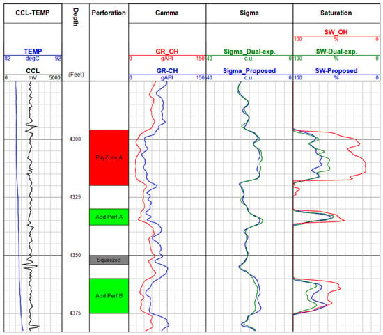
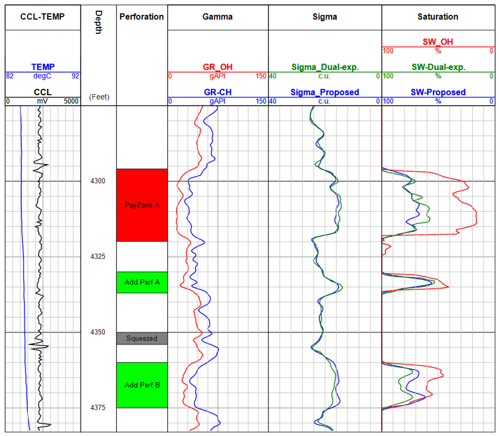
Well X is a mature producing well in an oilfield that was put into production in 2005. To identify additional potentially productive intervals, a pulsed neutron lifetime logging survey was conducted. After preprocessing of the logging data, formation water saturation was calculated using a volumetric model. Based on the resulting water-saturation interpretation, additional perforation operations were subsequently performed. Figure 16 shows the pulsed neutron lifetime logging curves acquired in Well X.

Figure 17 presents the PNL interpretation results for Well X. Track 1 shows the well-temperature and casing-collar locator (CCL) curves, Track 2 shows depth, Track 3 indicates the perforated intervals, and Track 4 displays the gamma-ray curves. Track 5 presents the Sigma curves, whereas Track 6 shows the water-saturation results calculated from Sigma. In Track 5, Sigma_Dual-exp was obtained using the double-exponential fitting method, whereas Sigma_Proposed was calculated using the method proposed in this study. In Track 6, SW_OH represents the original formation water saturation interpreted from open-hole logs acquired during the initial well-completion stage and is used as a historical reference; SW_Dual-exp represents the current water saturation calculated from the Sigma obtained by double-exponential fitting, whereas SW_Proposed represents the current water saturation calculated from the Sigma obtained using the proposed method.

Figure 17. The interpretation result map of PNL for Well X.

Pay Zone A is a producing interval that has remained on production for an extended period. Both SW_Dual-exp. and SW_Proposed are higher than SW_OH, with SW_Dual-exp. being slightly lower than SW_Proposed. However, field production data indicate that the current water cut of Pay Zone A is close to 90%, suggesting that the SW_Proposed result is more consistent with the actual production performance. In the Add Perf A interval, the water-saturation estimates obtained by the two methods show no obvious difference and are both relatively low; therefore, this interval was selected for additional perforation and subsequently put into production. In the Add Perf B interval, both SW_Dual-exp. and SW_Proposed are lower than SW_OH. A neighboring well had already produced from the corresponding interval for approximately six months, with a produced-fluid water cut of about 80%. SW_Dual-exp. is noticeably higher than SW_Proposed, and, considering the neighboring-well production data, the interpretation team considered SW_Proposed to be more consistent with the actual reservoir performance. Additional perforation was therefore recommended for this interval. After the Add Perf A and Add Perf B intervals were perforated, subsequent metering showed that the produced-fluid water cut decreased to 76%, while the wellhead daily oil production increased by 109 m³/d.

5. Conclusions

This study developed a physics-constrained time-spectrum processing framework for pulsed neutron lifetime logging based on borehole–formation separation and bidirectional constraints. Rather than simultaneously estimating the borehole and formation decay components from a mixed spectrum using conventional double-exponential fitting, the proposed method converts the problem into an alternating single-component reconstruction process. The borehole component is reconstructed from its characteristic early-time decay behavior and used to update the formation component, while the updated formation component is subsequently used to constrain the borehole component. The measured-spectrum superposition relationship, single-component exponential-decay behavior over selected characteristic intervals, and non-negativity of the separated components are incorporated as physical constraints. Iteration is terminated when the formation sigma satisfies the prescribed convergence criterion or when further updating produces a physically inadmissible negative component.

Monte Carlo simulations were used to investigate the temporal distributions of the borehole- and formation-region responses and to validate the proposed separation framework. The results show that borehole size and borehole-fluid salinity mainly affect the relative borehole–formation contributions and count levels, whereas formation lithology, porosity, and formation-water salinity have more pronounced effects on the formation decay characteristics. Within the effective analysis interval, the formation-region contribution generally remained below approximately 40%, confirming that substantial borehole contributions persist even in time intervals suitable for formation-sigma estimation and that temporal-window selection alone cannot completely isolate the formation response. The simulation results further support the use of approximately 600–1300 μs as a reference formation-sensitive interval for initializing formation-component fitting under the investigated conditions, while the fitting cutoff may be advanced for rapidly decaying formations to reduce the influence of late-time statistical fluctuations and accelerate convergence.

Direct comparison with Monte Carlo region-selective gamma-ray production formation-region spectra demonstrated that the proposed method can effectively recover the formation-component decay behavior. Across five validation models, the relative errors of apparent-sigma estimation were below 0.034% for the near detector and below 0.026% for the far detector, compared with 1.25–8.20% and 0.32–11.67%, respectively, for conventional double-exponential fitting. After applying the same multi-detector correction procedure, the proposed method provided more accurate formation-sigma estimates for all five validation models, reducing the mean relative error from approximately 5.19% for double-exponential fitting to 0.78%.

Application to field logging data from a mature producing well further demonstrated the practical utility of the method. The water-saturation results derived from the proposed formation-sigma estimates were more consistent with available production information in key intervals and supported the selection of additional perforation zones. Following additional perforation of the selected intervals, the produced-fluid water cut decreased to 76%, while daily wellhead oil production increased by 109 m³/d. These results indicate that the proposed framework provides a promising approach for improving PNL time-spectrum interpretation under complex borehole and formation conditions. Further work should focus on refining adaptive interval-selection criteria and validating the method using a broader range of field data.

References

- Qu, Y.; Pei, C.; Li, W.; Yu, Z.; Zhong, X.; Tan, M.; Zhang, T. Thermal Neutron Imaging Log Interpretation and Classification Methods for Water-Flooded Reservoirs. Geophys. Prospect. Pet. 2022, 61, 743–749. [Google Scholar] [CrossRef]
- Mauborgne, M.L.; Allioli, F.; Cao Minh, C.C.; Griffiths, R.; Maeso, C.; Reichel, N.; Stoller, C.; Murray, D.; Prabawa, H.; Haggag, M.; et al. Advances in LWD Multiple Depth of Investigation Array Sigma Measurements. In Proceedings of the SPWLA 54th Annual Logging Symposium, New Orleans, LA, USA, 22–26 June 2013; Paper No. SPWLA-2013-III; Society of Petrophysicists and Well-Log Analysts (SPWLA): Houston, TX, USA, 2013. [Google Scholar]
- Ali, A.; Small, S.; Singh, K.; Martin, A. Significance of Time-Lapsed Hydrocarbon Saturations from Pulsed-Neutron-Capture (PNC) Logs and the Impact of Borehole-Environment Parameters on PNC-Derived Saturations. SPE Reserv. Eval. Eng. 2017, 20, 285–292. [Google Scholar] [CrossRef] [Scilit]
- Yu, B.; Ito, K.; Miles, J.; Rasmus, J.; Xie, H.; Sun, K.; Abubakar, A. An Improved Fast Forward-Modeling Technique for Logging While Drilling Sigma Measurements. In Proceedings of the SEG Technical Program Expanded Abstracts 2017, Houston, TX, USA, 24–29 September 2017; pp. 905–909. [Google Scholar] [CrossRef] [Scilit]
- Mickael, M.W. A New Algorithm for Correcting Neutron Decay Logs for Borehole and Diffusion Effects. Log. Anal. 1999, 40, 471–478. [Google Scholar]
- Li, Q.; Zhang, G.; Cao, H.; Li, Q.; Wang, F.; Wu, J.; Chen, W.; Ma, W. Multiphysics Modeling and Microscopic Analysis of Water-Based Heat Extraction from Hot Dry Rock Reservoirs. Energies 2026, 19, 4513. [Google Scholar] [CrossRef] [Scilit]
- Ao, F.; Li, Q.; Li, Q.; Wu, J.; Wang, F.; Yan, C. Numerical Simulation Investigation of Fracture Propagation Behavior Patterns and Sensitivity Factors of Oil Shale Reservoirs in the Xunyi Region Considering the Influence of Natural Fracture. Geofluids 2025, 2025, 2762142. [Google Scholar] [CrossRef] [Scilit]
- Wu, J.; Li, Q.; Li, Q.; Wang, F.; Cheng, Y.; Yan, C. Design and Optimization of Bottom-Hole Temperature–Pressure Combinations in Gas Production from Gas Hydrates via Carbon Dioxide Replacement Strategy. Energies 2026, 19, 3536. [Google Scholar] [CrossRef] [Scilit]
- Tian, L.; Zhang, F.; Wu, Z.; Wang, Z.; Qiu, F.; Fang, Q.; Chen, Q.; Zhou, L. A New Diffusion Effect Correction Method in Pulsed Neutron Capture Logging. J. Pet. Sci. Eng. 2021, 204, 108673. [Google Scholar] [CrossRef] [Scilit]
- Qiu, F.; Zhang, F.; Zhang, X.; Chen, Q.; Fan, J.; Lu, B. A study on characteristics of background gamma spectrum from LaCl3 detector in pulsed neutron logging. Appl. Radiat. Isot. 2023, 195, 110738. [Google Scholar] [CrossRef] [Scilit] [PubMed]
- Youmans, A.H.; Hopkinson, E.C.; Bergan, R.A.; Oshry, H.I. Neutron Lifetime, a New Nuclear Log. J. Pet. Technol. 1964, 16, 319–328. [Google Scholar] [CrossRef] [Scilit]
- Tittman, J.; Nelligan, W.B. Laboratory Studies of a Pulsed Neutron-Source Technique in Well Logging. J. Pet. Technol. 1960, 12, 63–66. [Google Scholar] [CrossRef] [Scilit]
- Randall, R.R.; Oliver, D.W.; Fertl, W.H. The PDK-100 Enhances Interpretation Capabilities for Pulsed Neutron Capture Logs. In Proceedings of the SPWLA 27th Annual Logging Symposium, Houston, TX, USA, 9–13 June 1986. Paper No. SPWLA-1986-JJJ. [Google Scholar]
- Rose, D.; Zhou, T.; Beekman, S.; Quinlan, T.; Delgadillo, M.; Gonzalez, G.; Fricke, S.; Thornton, J.; Clinton, D.; Gicquel, F.; et al. An Innovative Slim Pulsed Neutron Logging Tool. In Proceedings of the SPWLA 56th Annual Logging Symposium, Long Beach, CA, USA, 18–22 July 2015. [Google Scholar]
- Zhou, P.; Tang, B. Experimental Study of the Influence of Borehole Parameters on Prompt Fission Neutron Uranium Logging and Its Corrections. Nucl. Eng. Technol. 2024, 56, 3090–3096. [Google Scholar] [CrossRef] [Scilit]
- Gyllensten, A.; Al-Arfi, S.; Al Hammadi, M.; Al Marzouqi, K.; Madjidi, A.; Mauborgne, M.-L.; Weller, G. Advances in LWD Sigma Measurements and Application to Real-Time Formation Evaluation in Carbonate Reservoirs. In Proceedings of the SPWLA 50th Annual Logging Symposium, The Woodlands, TX, USA, 21–24 June 2009. Paper No. SPWLA-2009-26949. [Google Scholar]
- Zhang, Q.; Zhang, G.; Deng, R.; Zhang, F.; Zhu, K.; Luo, X. Time-Spectrum Processing Technology of Neutron Lifetime Logging Based on Regularized Non-Negative Least Squares Method. J. Pet. Sci. Eng. 2021, 203, 108604. [Google Scholar] [CrossRef] [Scilit]
- Li, F.; Han, X.; Mendez, F. Sigma Measurement and Applications with a Pulsed-Neutron Mineralogy Instrument. In Proceedings of the SPWLA 52nd Annual Logging Symposium, Colorado Springs, CO, USA, 14–18 May 2011. Paper No. SPWLA-2011-YYY. [Google Scholar]
- Al-Turkey, S.; Freile, D.; Tagarieva, L.; Elyas, M.; Schmid, G. Diffusion-Corrected Sigma Using Dual Exponential Fit for Time-Lapse Reservoir Monitoring. In Proceedings of the International Petroleum Technology Conference, Dhahran, Saudi Arabia, 13–15 January 2020. Paper No. IPTC-19915-MS. [Google Scholar] [CrossRef] [Scilit]
- Schmid, G.; Pemper, R.; Dolliver, D.; Mekic, N.; Musselman, J. A Diffusion-Corrected Sigma Algorithm for a Four-Detector Pulsed-Neutron Logging Tool. In Proceedings of the SPE Annual Technical Conference and Exhibition, Dallas, TX, USA, 24–26 September 2018. Paper No. SPE-191738-MS. [Google Scholar] [CrossRef] [Scilit]
- Li, Y.; Wang, X.; Chang, J. Theory and Examples of the Interaction between Neutron Sources and Formations. Pet. Instrum. 2009, 23, 68–69+76. [Google Scholar]
- Ortega, E.; Torres-Verdín, C.; Preeg, W.E. Rapid Forward Modeling of Multidetector Logging-While-Drilling Sigma Measurements. Geophysics 2014, 79, D253–D273. [Google Scholar] [CrossRef] [Scilit]
- Mauborgne, M.-L.; Allioli, F.; Stoller, C.; Evans, M.; Manclossi, M.; Nicoletti, L. Exploring for oil with nuclear physics. EPJ Web Conf. 2017, 146, 09009. [Google Scholar] [CrossRef] [Scilit]
- Wahl, J.S.; Nelligan, W.B.; Frentrop, A.H.; Johnstone, C.W.; Schwartz, R.J. The Thermal Neutron Decay Time Log. SPE J. 1970, 10, 365–379. [Google Scholar] [CrossRef] [Scilit]
- Odom, R.C.; Bailey, S.M.; Wilson, R.D. Benchmarking computer simulations of neutron-induced, gamma-ray spectroscopy for well logging. Appl. Radiat. Isot. 1997, 48, 1321–1328. [Google Scholar] [CrossRef] [Scilit]
- Gilchrist, A.; Trcka, D.E. Apparatus and Method for Determining Thermal Neutron Capture Cross Section of a Subsurface Formation from a Borehole Using Multiple Detectors. U.S. Patent 7,253,402, 7 August 2007. [Google Scholar]
- Zhang, Q.; Ge, Y.; Li, Y.-L. Source-less density measurement using an adaptive neutron-induced gamma correction method. Nucl. Sci. Tech. 2023, 34, 125. [Google Scholar] [CrossRef] [Scilit]
Disclaimer/Publisher’s Note: The statements, opinions and data contained in all publications are solely those of the individual author(s) and contributor(s) and not of MDPI and/or the editor(s). MDPI and/or the editor(s) disclaim responsibility for any injury to people or property resulting from any ideas, methods, instructions or products referred to in the content. |
© 2026 by the authors. Licensee MDPI, Basel, Switzerland. This article is an open access article distributed under the terms and conditions of the Creative Commons Attribution (CC BY) license.