DSF-YOLO: Multi-Scale Fire and Smoke Detection Based on YOLO11

Abstract

Detecting fire and smoke across a wide range of object sizes requires both spatial detail and contextual information. However, incorporating these features into a compact detector remains a challenge. This study presents DSF-YOLO, a fire and smoke detector based on YOLO11n. C3K2-MFB introduces wavelet processing into C3K2 to represent coarse structures and fine details in separate frequency subbands. DyFusion Block combines local convolutional features with transformer-based context to support complementary feature processing. ADown is also introduced to reduce the cost of downsampling. For bounding-box regression, AIM-MSAIoU combines auxiliary-box overlap at a fixed scale of 0.7 with a shape-weighted corner penalty normalized by target size. The model is evaluated on the Dual-Scale Fire (DSF) dataset, which contains 7572 images and four scale-based fire and smoke classes. Compared with YOLO11n, DSF-YOLO increases mAP@0.5 from 0.905 to 0.919 and mAP@[0.5:0.95] from 0.631 to 0.680. At the same time, parameter count decreases by 8.14% to 2.37 M, and FLOPs decrease by 4.76% to 6.0 G FLOPs. Reported throughput increases from 164.0 to 175.0 FPS on an RTX 4090D at a batch size of 16. The results show that DSF-YOLO improves detection accuracy while reducing computational cost under the reported conditions.

1. Introduction

Early detection of fire and smoke can support a timely response to threats to life and property [1]. Advances in imaging and deep learning have therefore encouraged research into vision-based fire monitoring [1,2]. Object detectors commonly follow either a two-stage or a one-stage design. Two-stage detectors, such as Faster R-CNN [3], generate candidate regions before classifying them and refining their bounding boxes. In contrast, one-stage detectors, such as YOLO [4], predict object classes and locations in a single forward pass. This unified prediction process makes one-stage detection relevant to continuous monitoring, where both detection accuracy and processing speed matter.

YOLO established a unified, single-pass prediction of object locations and classes [4]. Later versions introduced multi-scale prediction and feature aggregation for objects of different sizes: YOLOv3 predicts at several feature-map resolutions [5], and YOLOv4 and YOLOv5 further develop extraction and aggregation strategies [6,7]. Feature fusion has advanced in parallel, from the top-down pathway of Feature Pyramid Networks [8] and the bottom-up path of Path Aggregation Network [9] to the weighted bidirectional fusion of EfficientDet [10]. Recent detectors explore different forms of feature interaction, including attention-centric YOLOv12 [11] and hypergraph-based YOLOv13 [12]; the compact YOLO26n [13] is also included in this study as a comparison model. These architectures provide a range of reference designs for assessing the accuracy and computational cost of task-specific modifications.

Despite these advances, fire and smoke introduce challenges that are not fully described by object size alone. Flame appearance changes across combustion stages, and smoke may have diffuse boundaries, low contrast and partial transparency. Viewing distance also produces large-scale differences, from small, distant flames to broad smoke plumes [1,14,15,16]. Recent studies address these difficulties through both feature design and training supervision. YOLO-Fire adds a P2 detection layer and coordinate attention for multi-scale fire detection [17,18]. SFFA-YOLO combines cross-scale feature fusion, channel–spatial feature processing and dynamic supervision for fire and smoke targets [19]. Other studies investigate compact convolutional networks and attention-based feature processing to balance recognition performance and computational cost [20,21,22,23,24]. These approaches provide useful design directions, but small smoke regions remain difficult to distinguish from clouds, haze and other visually similar objects [16,25]. Thus, increasing feature resolution alone may be insufficient: the detector also needs contextual information to interpret weak local evidence. This requirement is particularly relevant to continuous monitoring, where additional feature processing must be considered alongside inference cost.

These observations motivate a detector that combines spatial detail, broader context and suitable localization supervision within a compact architecture. Multi-scale fusion can bring low-level localization cues together with high-level semantic information [9,10], but its benefit depends on how features are processed and how much computation is added. We therefore develop DSF-YOLO from YOLO11n, with coordinated changes to feature extraction, feature interaction, downsampling and bounding-box regression. Wavelet processing provides separate representations of coarse structures and detail; local and Transformer branches combine complementary information; ADown limits downsampling cost; the revised regression objective supervises box overlap and corner alignment. The contributions are summarized as follows:

(1)

C3K2-MFB introduces wavelet processing into C3K2, using frequency subbands to represent coarse spatial structures and fine details within the feature extraction stage.

(2)

DyFusion Block combines a local convolutional branch with a Transformer branch, allowing local features and broader contextual information to be processed within one block.

(3)

AIM-MSAIoU combines fixed-scale auxiliary-box overlap with a shape-weighted corner penalty normalized by target size, providing complementary constraints for bounding-box regression.

Section 1 introduces the background and motivation of this study. Section 2 describes the model architecture and its components. Section 3 presents the datasets, experimental settings, comparative results and ablation analysis. Section 4 discusses the conclusions and remaining limitations.

2. Proposed Method

YOLO11 is a one-stage detector whose architecture includes C3k2 feature-extraction modules and C2PSA for contextual feature interaction [26]. Its backbone extracts features at successive spatial resolutions, while the neck combines information for detection at multiple scales. We use YOLO11n as the baseline because these components provide suitable locations for introducing frequency processing, contextual modeling and more economical downsampling. This common starting point allows each modification to be examined through matched ablation configurations. The complete model is compared with lightweight YOLO variants, including YOLOv12 and YOLOv13 [11,12], under the reported experimental settings.

Fire and smoke detection present several related challenges: weak or blurred local boundaries, background patterns with similar appearances, and large differences in object size. Repeated downsampling can also remove spatial information needed to localize small objects. Together, these challenges motivate complementary changes in feature representation and box supervision: local detail and scene context support recognition, while the downsampling strategy and regression objective influence the information available for localization.

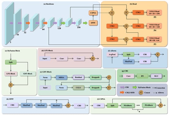
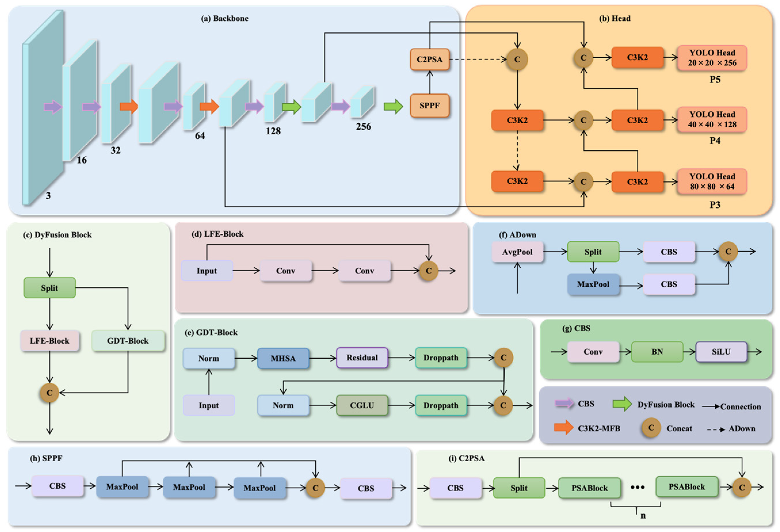
To address these challenges, DSF-YOLO introduces four changes to the YOLO11n framework (Figure 1). C3K2-MFB combines wavelet decomposition with learnable filtering and channel weighting to represent coarse structures and local detail. DyFusion Block then complements local convolutional processing with self-attention, allowing features from different positions to interact. ADown replaces selected downsampling operations with a two-branch channel structure to reduce convolutional cost. Finally, AIM-MSAIoU modifies box-regression supervision using auxiliary-box overlap and shape-weighted corner distances. The first three changes affect feature processing, whereas the loss acts during training. Their separate and combined effects are evaluated in the ablation study.

Figure 1. Overall architecture of DSF-YOLO: (a) backbone, in which C3K2-MFB (orange) and DyFusion Block (green) mark the modified stages; (b) head, with detection heads at the P3, P4 and P5 levels and ADown shown as dashed paths; (c) DyFusion Block; (d) LFE-Block; (e) GDT-Block, combining an MHSA path and a CGLU path through residual addition and DropPath; (f) ADown; (g) CBS; (h) SPPF; and (i) C2PSA. C denotes channel concatenation. P3–P5 denotes feature-pyramid levels; channel widths are schematic.

2.1. C3K2-MFB

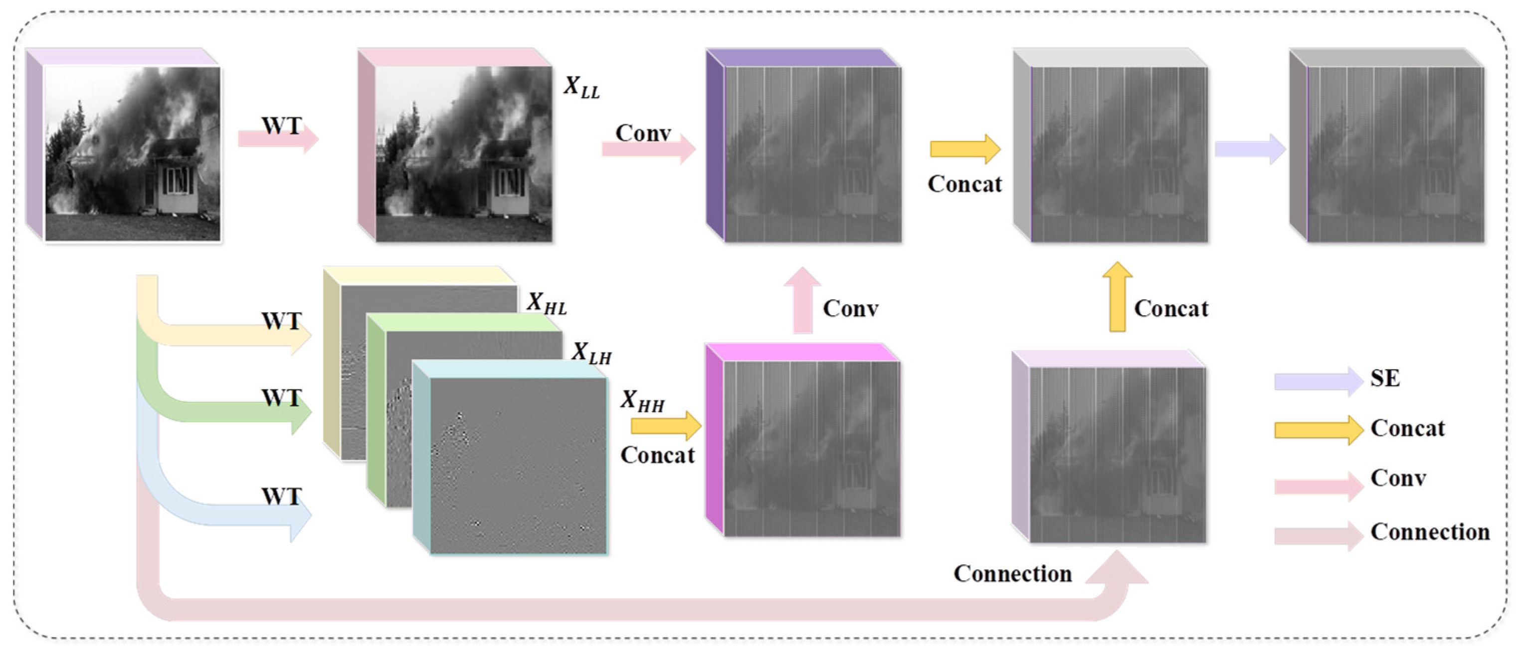
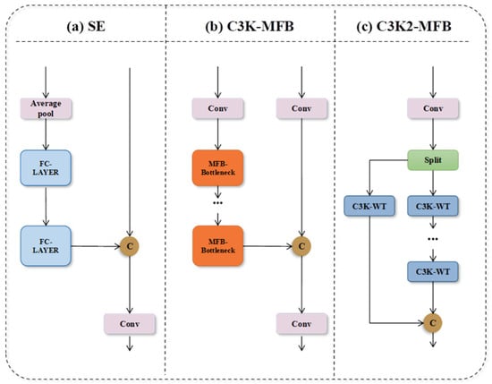
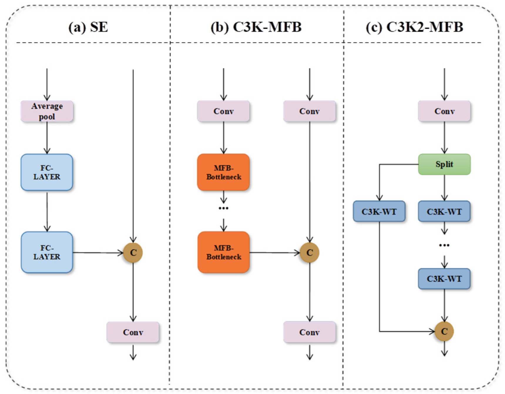
Fire and smoke may contain both broad, slowly varying regions and fine boundary or texture changes. A single spatial scale may, therefore, provide an incomplete description of their appearance. C3K2-MFB introduces wavelet processing into C3K2 to represent these components at multiple resolutions. Wavelet decomposition separates an approximation component from directional detail components [27], while learnable filtering and inverse reconstruction follow the wavelet-convolution principle [28]. SE subsequently adjusts channel responses according to the input [29]. Input connections allow frequency-processed information to be combined with spatial features. The resulting representation is intended to retain structural cues at different scales for subsequent detection.

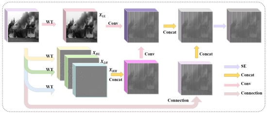
Figure 2 and Figure 3 show the frequency-processing path and its integration into C3K2-MFB. A two-dimensional wavelet transform produces an approximation band, LL, and three detail bands: LH, HL and HH. LL represents coarse spatial variation, whereas the detail bands describe changes along different directions; these bands do not correspond directly to object categories. For multilevel analysis, the LL component is decomposed again, providing access to progressively coarser structure. In Equation (1), Conv denotes fixed wavelet filtering with downsampling, not the learnable convolution subsequently applied to the sub-bands. This distinction separates the decomposition operation from feature learning:

[X_LL,X_LH,X_HL,X_HH] = Conv([f_LL,f_LH,f_HL,f_HH],X)

(1)

Figure 2. Conceptual frequency-processing path in the MFB bottleneck. Approximation and detail bands undergo learnable filtering and inverse reconstruction before feature combination and channel recalibration.

Figure 3. Component schematics: (a) SE channel weighting; (b) C3K-MFB; and (c) C3K2-MFB. SE multiplies channels by learned weights; the C3K branches use feature concatenation. Repetition counts and channel widths are omitted.

The filters f_LH, f_HL, f_HH and f_LL generate the four sub-bands. Equation (2) describes recursive decomposition, initialized with $X_{\mathit{LL}}^{\left(0\right)}=X$. Equation (3) illustrates a single level of wavelet-domain filtering with learnable weights W followed by inverse reconstruction. With multiple decomposition levels, reconstruction proceeds from coarse to fine [28]; Equation (3) alone is therefore not a complete specification of a multilevel implementation.

$$\{X_{\mathit{LL}}^{\left(i\right)},X_{\mathit{LH}}^{\left(i\right)},X_{\mathit{HL}}^{\left(i\right)},X_{\mathit{HH}}^{\left(i\right)}\}=\mathit{WT}\left(X_{\mathit{LL}}^{(i-1)}\right)$$

(2)

Y = IWT(Conv(W ⋅ WT(X)))

(3)

SE first applies global average pooling to obtain one descriptor per channel. Two fully connected layers then reduce the descriptor dimension from C to C/r and restore it to C, with a nonlinear activation between the layers and a final sigmoid. The resulting weights multiply the corresponding feature channels [29]. For example, C = 256 and r = 16 give a 16-dimensional hidden representation; this example does not prescribe the channel dimensions at every stage. Within C3K2-MFB, channel weighting complements wavelet processing by adjusting the contributions of the reconstructed features. The combined module is used in backbone feature extraction.

2.2. DyFusion Block

Frequency processing can describe local variation, but local appearance alone may remain ambiguous when background regions resemble fire or smoke. Relating a candidate region to its surroundings provides an additional source of information [14,15,16,21,22]. This motivates the contextual branch introduced in DyFusion Block.

Self-attention models dependencies between feature positions [30,31]. Hierarchical visual Transformers also demonstrate ways of organizing contextual processing while controlling its cost [32], although the cost depends on the attention design and input resolution. Following this motivation, DyFusion Block combines a Local Feature Extraction Block (LFE-Block) with a Global Dependency Transformer Block (GDT-Block) (Figure 4). The input features are split into two branches, processed separately and then combined. The local branch captures nearby spatial patterns, while the attention branch enables interaction across positions. Combining these branches is intended to retain local evidence and use scene context to help distinguish target regions from similar background appearances.

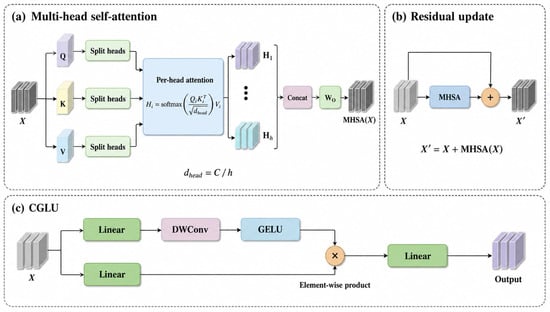
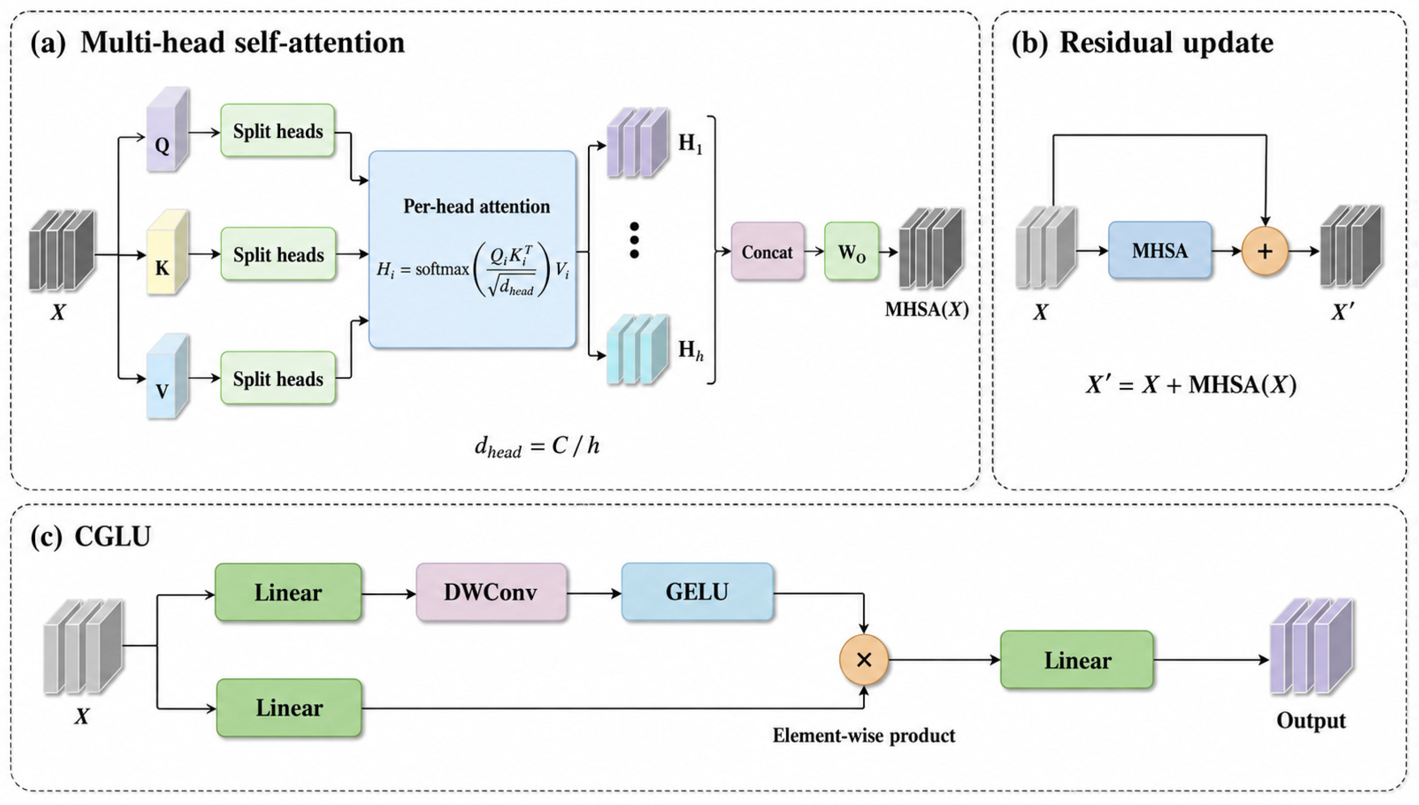
Figure 4. GDT-Block principles: (a) multi-head self-attention; (b) residual addition; and (c) convolutional GLU [30,33]. Normalization and training-time DropPath are omitted in this schematic.

LFE-Block applies two 3 × 3 convolutions and combines their output with the input features. The input connection carries intermediate features alongside the convolutional path. GDT-Block contains multi-head self-attention (MHSA) followed by a convolutional gated linear unit (CGLU). In GDT-Block, normalized features are projected into queries Q, keys K and values V. Following the multi-head attention formulation [30], these projections are partitioned into h heads. Within each head, query–key similarities determine the attention weights, which are applied to the values. The scaled dot-product operation is:

$${\mathit{Attention}}_i=\mathit{Softmax}(Q_i{K}_i^T/\sqrt{d_{\mathit{head}}})\cdot V_i$$

(4)

d_head = c/h is the feature dimension of each head, with C divisible by h. The outputs of all heads are concatenated and mapped by the output projection W_O:

MultiHead(Q,K,V) = Concat(Attention₁,…,Attention_h)W_O

(5)

The projected attention output is combined with the input through a residual connection. DropPath denotes stochastic depth applied to the attention branch during training. The addition in Equation (6) combines the input representation with attention-derived information; reshaping between feature maps and token sequences is a separate operation:

X_out = X + DropPath(MultiHead(Q,K,V))

(6)

The residual output therefore contains value features weighted by dependencies across positions. CGLU complements this interaction with local processing and multiplicative gating. In the cited CGLU formulation, one projected branch passes through a depthwise convolution and GELU before multiplying the other branch; an output projection follows [33]. This introduces local spatial information into the gate, complementing the interactions modeled by self-attention. DyFusion is used in deeper feature processing, where lower spatial resolution helps limit the cost of attention. Its contribution to detection is assessed through the corresponding ablations.

2.3. ADown

Feature enrichment also requires attention to computational cost. As shown by the module-level ablation (Section 3.4.1), the standalone DyFusion and C3K2-MFB variants have slightly fewer parameters and FLOPs than YOLO11n, but their reported throughput falls from 164.0 FPS to 141.7 and 104.5 FPS, respectively. These values correspond to throughput reductions of 13.6% and 36.3%. We therefore adopt ADown from YOLOv9 to reduce the convolutional cost of selected downsampling operations [34].

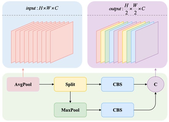
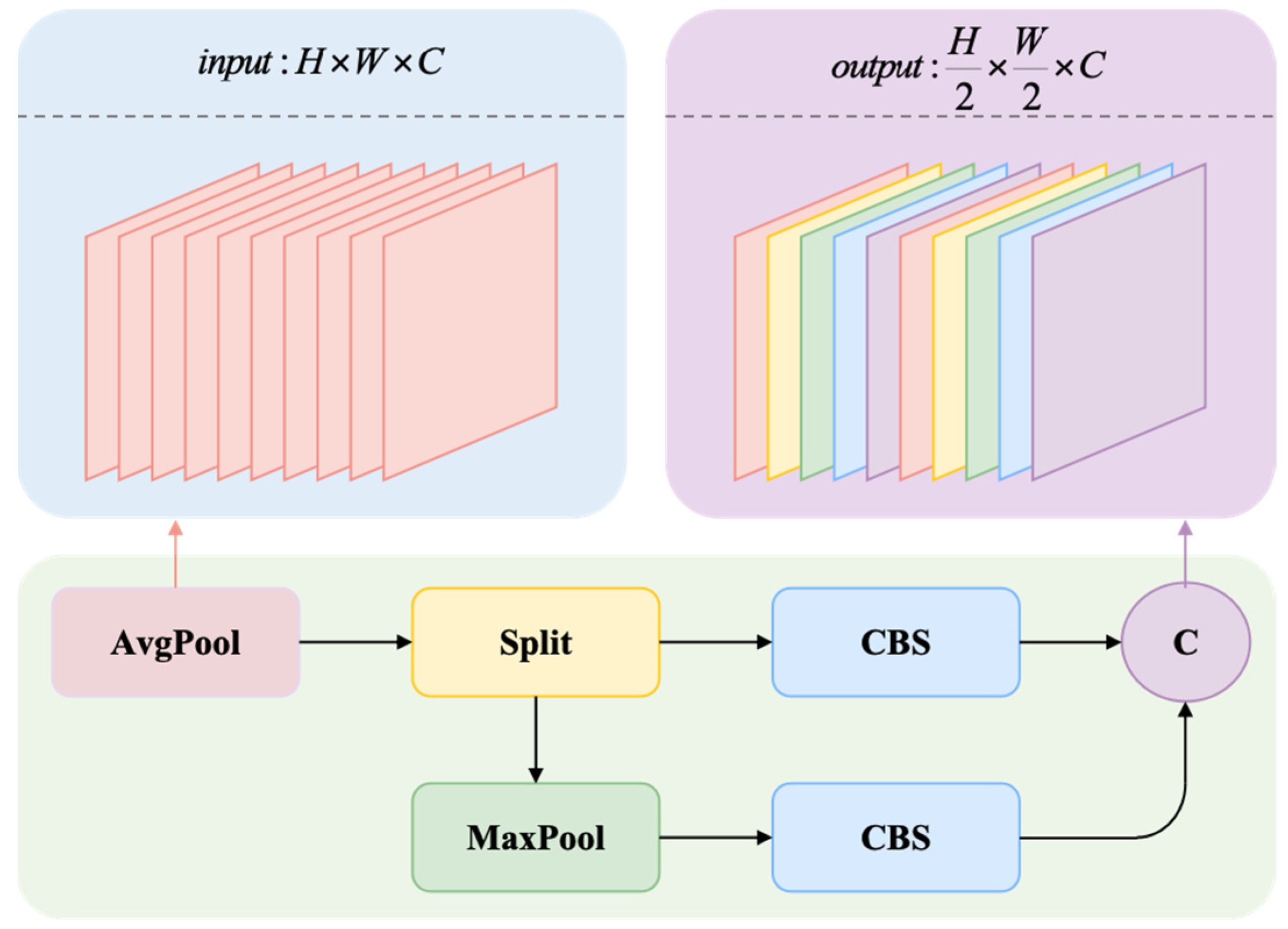
Given an input of size H × W × C_in and even input and output channel counts, ADown first applies 2 × 2 average pooling with stride 1 and no padding (Figure 5). The result is divided equally along the channel dimension. One branch uses a 3 × 3 convolution with stride 2 and padding 1. The other uses 3 × 3 max pooling with stride 2 and padding 1, followed by a 1 × 1 convolution. The convolutions include batch normalization and SiLU activation. Concatenating the branch outputs gives C_out channels and, for even H and W, spatial dimensions H/2 × W/2. The configured C_out need not equal C_in.

Figure 5. ADown operations [34]. Each branch processes half of the input channels and produces half of the output channels. CBS denotes convolution, batch normalization and SiLU activation.

Compared with applying a full-channel 3 × 3 stride-2 convolution, ADown can lower convolutional cost because each branch processes only half of the input channels and the pooling branch uses a 1 × 1 convolution [34]. The branches also apply different spatial transformations: one learns a strided filter, while the other selects local maxima before channel mixing. Their outputs are combined to retain complementary information, although downsampling still reduces spatial resolution. In DSF-YOLO, ADown replaces the P3–P4 and P4–P5 downsampling transitions. Its effect on accuracy and throughput depends on the surrounding modules and is therefore examined for each ablation configuration, rather than inferred from FLOPs alone.

2.4. AIM-MSAIoU

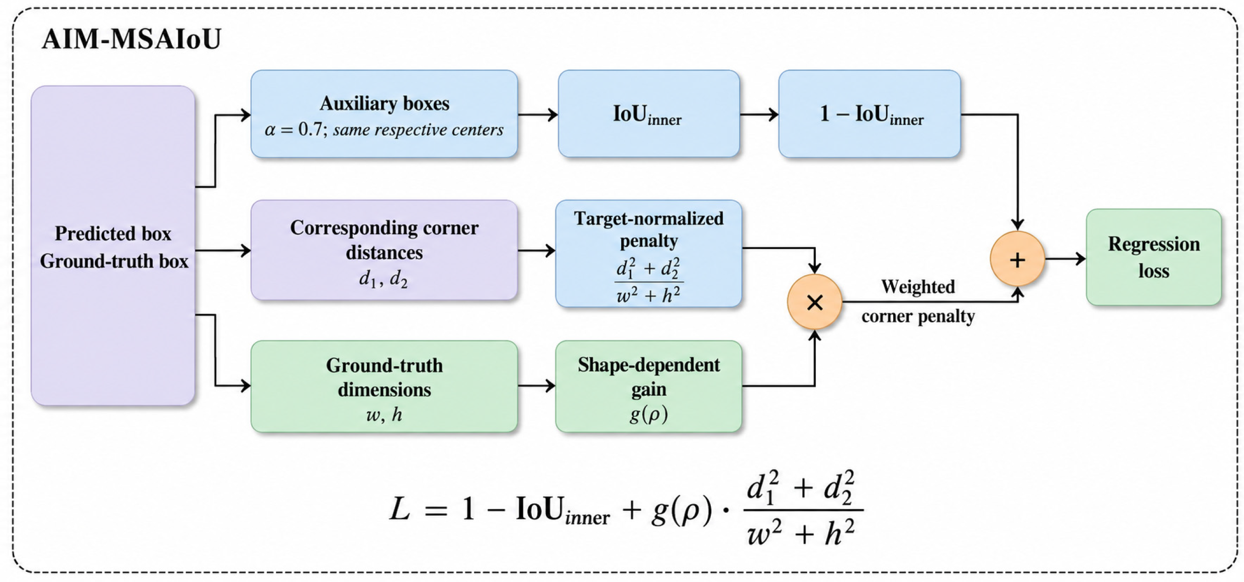
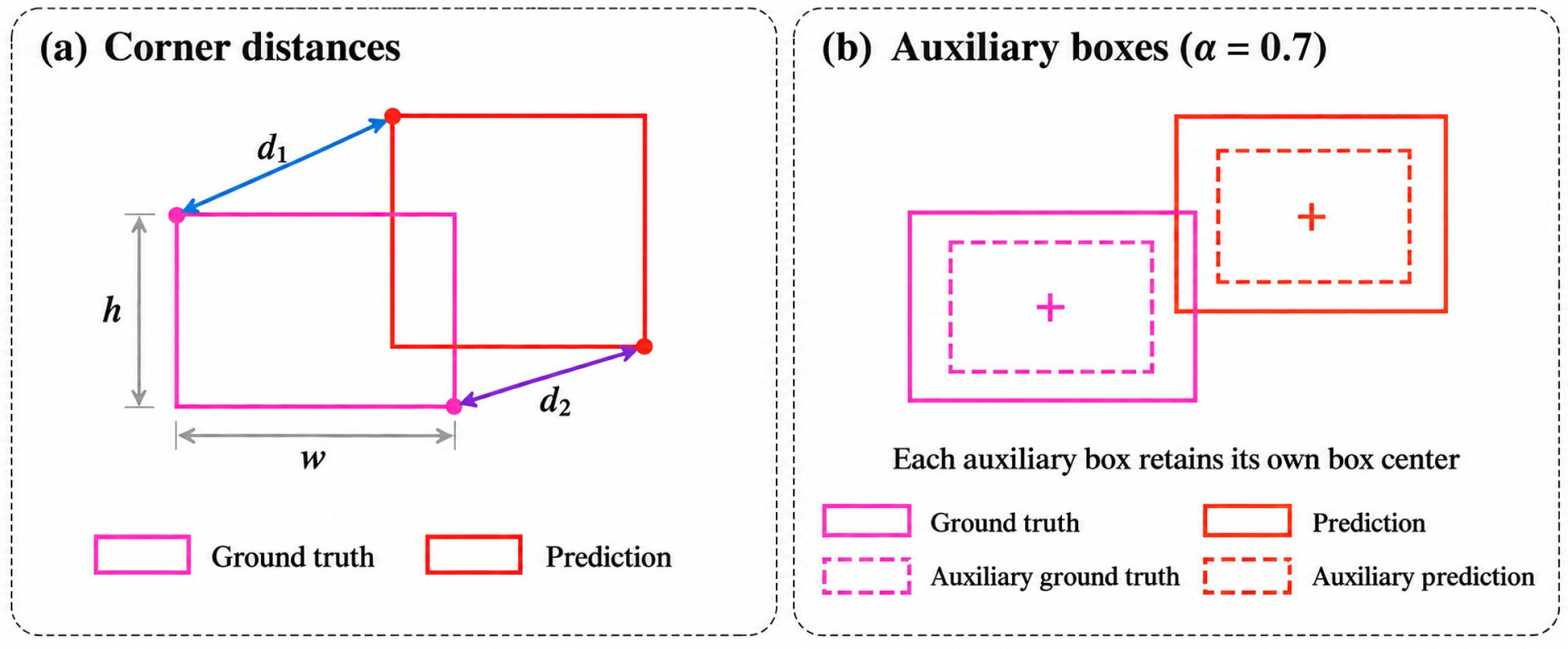
Bounding-box regression measures geometric agreement between predicted and ground-truth rectangles. IoU-based extensions introduce additional signals for different overlap conditions [35]. CIoU combines overlap, center distance and aspect ratio [36]. However, when two boxes share an aspect ratio, its ratio term does not directly measure differences in their absolute widths and heights; the overlap and center-distance terms still provide supervision. This motivates using corresponding corners to describe residual position and size errors. For fire and smoke, whose annotated extents may be difficult to localize, AIM-MSAIoU combines this corner supervision with auxiliary-box overlap. It remains a loss for axis-aligned bounding boxes and does not directly represent irregular object contours. Figure 6 summarizes its components.

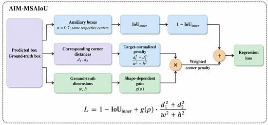
Figure 6. AIM-MSAIoU components in Equations (7) and (8). The loss combines one minus auxiliary-box IoU with a shape-weighted, target-normalized corner penalty; it contains no separate angular-cost term.

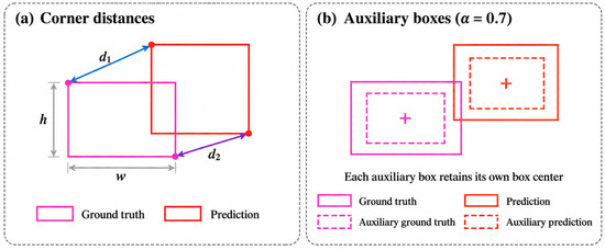
AIM-MSAIoU combines the corner-distance principle of MPDIoU [37] with the auxiliary-box strategy of Inner-IoU [38]. In this manuscript, MSAIoU denotes the corner-based variant normalized by target dimensions. The top-left and bottom-right corners jointly determine an axis-aligned box, so their distances provide supervision for both position and size errors (Figure 7a). This use of corresponding corners differs from explicitly penalizing only the distance between box centers.

Figure 7. Loss geometry: (a) corresponding top-left and bottom-right corner distances, with ground-truth width w and height h; and (b) auxiliary boxes scaled about their respective centers by α = 0.7.

For the overlap component, each predicted and ground-truth box is scaled about its own center, with its width and height multiplied by the fixed ratio α = 0.7 (Figure 7b). The resulting auxiliary boxes are used to compute IoU_inner. Shrinking the boxes can increase sensitivity when their overlap is already high, but also reduces the range over which they overlap [38]. The fixed ratio therefore controls a trade-off between the effective overlap range and sensitivity to the alignment of already overlapping boxes. The loss is defined as:

$$L_{\mathit{AIM}-\mathit{MSAIoU}}=1-{\mathit{IoU}}_{\mathit{inner}}+\left[a_1\sigma \left(\rho \right)+\left(1-\sigma \left(\rho \right)\right)a_2\right]\cdot {\displaystyle \frac{d_1^2+d_2^2}{w^2+h^2}}$$

(7)

The logistic mixing function is defined as:

$$\sigma (\rho )={\displaystyle \frac{1}{1+\mathit{exp}(-k(\rho -\tau \left)\right)}}$$

(8)

d₁ and d₂ are the distances between corresponding top-left and bottom-right corners. The positive quantities w and h are the ground-truth width and height. MPDIoU normalizes corner distances by the squared input-image diagonal [37], whereas Equation (7) uses w² + h² for the target. The penalty is consequently relative to target size and can become large for small boxes; the loss is not restricted to [0, 1].

The shape ratio ρ = |w − h|/max(w,h) lies in [0,1), equals zero for square boxes and approaches one as boxes become increasingly elongated. The gain g(ρ) = a₁σ(ρ) + a₂[1 − σ(ρ)] mixes two coefficients. For a non-negative corner penalty, g must remain non-negative over the admissible range; a₁,a₂ ≥ 0 are sufficient conditions. When k > 0, σ increases with ρ, so elongated targets receive greater gain only if a₁ > a₂. The parameters τ and k determine the transition location and slope. Training minimizes LAIM-MSAIoU in place of the CIoU term, while retaining the classification and distribution focal loss terms.

The resulting loss links auxiliary overlap to corner alignment and weights the corner error according to target geometry. Its adaptive element is this shape-dependent gain; the auxiliary-box ratio remains fixed, and no separate angular term is used. We evaluate this regression objective through the controlled loss comparison (Section 3.4.2) and the matched ablation configurations (Section 3.4.1).

3. Experimental Results and Analysis

3.1. Datasets

A dataset with explicit size labels was needed to evaluate fire and smoke detection across object scales. Public resources such as D-Fire [39], FASDD [40] and FLAME [41] provide imagery from different settings, but their labels and evaluation protocols should not be treated as interchangeable. We therefore constructed the Dual-Scale Fire (DSF) dataset using publicly available imagery and the Wildfire Smoke dataset released by AI for Mankind in collaboration with HPWREN [42]. Targets were outlined in LabelMe, and the polygons were converted to axis-aligned bounding boxes. Every image was named after its source and image index at collection time, so that the provenance of each image remains traceable throughout dataset construction. A second annotator checked all boxes, corrupted and near-duplicate images were removed, and a perceptual-hash comparison across sources was applied to exclude near-duplicates shared between different collections. To quantify annotation consistency, the second annotator independently re-annotated 250 images sampled proportionally from the four classes; 92.3% of the re-annotated boxes matched the released boxes at an IoU of at least 0.5, and the residual disagreements were concentrated on the outer boundaries of transparent smoke plumes.

An instance was defined as small when its bounding box occupied less than 1% of the area of the letterboxed 640 × 640 input, and combining this size rule with the fire and smoke categories produced four classes: large fire (LF), large smoke (LS), small fire (SF) and small smoke (SS). The 1% threshold was fixed before training by inspecting the distribution of annotated box-area ratios, which is bimodal and separates small from large instances in the vicinity of 1%; the threshold therefore lies at the natural boundary between the two modes rather than at a value selected for its effect on the reported results. For reference, 1% of the 640 × 640 evaluation input corresponds to a box area of 4096 pixels, which lies between the small and medium boundaries of the COCO area bands.

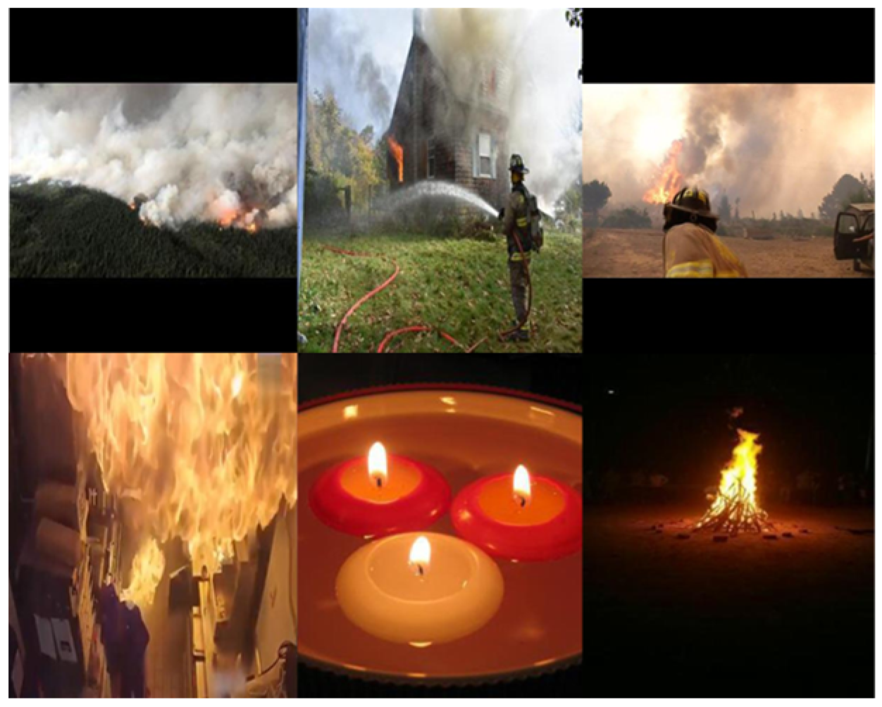
The resulting 7572 images were divided by source-level grouped splitting into training, validation and test subsets at an 8:1:1 ratio with a fixed seed: images sharing an HPWREN camera sequence, fire event, or originating dataset were assigned to a single subset, so that the training and test scenes are independent. The split lists and source-identifier manifest are available from the corresponding author upon reasonable request, and the previous random split at the same ratio is retained in Appendix A for comparison. Table 1 summarizes the number of images and instances of each class in each subset, and confirms that all four classes retain a sufficient number of instances in the validation and test subsets. This split was used throughout the DSF experiments. Figure 8 presents representative samples.

Table 1. Composition of the Dual-Scale Fire (DSF) dataset: number of images and instances per class in the training, validation, and test subsets under the source-grouped 8:1:1 split.

Class	Train Images	Val Images	Test Images	Train Instances	Val Instances	Test Instances	Total Instances
LF	2341	293	292	7152	894	894	8940
LS	2005	251	250	5772	722	721	7215
SF	1648	206	205	3506	438	438	4382
SS	1522	190	189	2889	361	361	3611
Total	6057	757	758	19,319	2415	2414	24,148

An image may contain instances of multiple classes; class-wise image counts therefore sum to more than the number of unique images. Instances are counted per bounding box.

Figure 8. DSF dataset sample figures.

Table 2 further examines the consequences of the class definition. Re-evaluating the class labels at thresholds of 0.5% and 2% changes mAP@0.5 by at most 0.2 percentage points and mAP@[0.5:0.95] by at most 0.5 points relative to the adopted threshold, indicating that the reported accuracy is insensitive to this choice. The instance counts vary monotonically with the threshold, as expected from the set-inclusion relation between the corresponding small-object sets. Table 3 reports size-stratified AP computed with the COCO area bands, an assessment independent of the class definition: DSF-YOLO improves over YOLO11n across all size bands, with the largest margin on small objects, as analyzed in Section 3.3.1. Because size is part of the class label, the resulting mAP evaluates a four-class detection task and should not be interpreted as conventional two-class fire and smoke accuracy or as an independently computed small-object AP; merged two-class results are reported in Section 3.3.1, and the native two-class benchmark results are reported in Section 3.3.2.

Table 2. Sensitivity of the class definition to the size threshold on the DSF test set.

Threshold	Small Instances	Large Instances	Small Share	mAP@0.5	mAP@[0.5:0.95]
0.5%	486	1928	20.1%	0.917	0.675
1.0%	799	1615	33.1%	0.919	0.680
2.0%	1214	1200	50.3%	0.920	0.681

The model is not retrained; ground-truth and predicted labels are re-merged by the same area-threshold rule before evaluation, so instance counts vary monotonically with the threshold.

Table 3. Size-stratified detection accuracy on the DSF test set, computed with the COCO area bands.

Size Band	GT Instances	YOLO11n AP@[0.5:0.95]	DSF-YOLO AP@[0.5:0.95]	Δ (pp)
Small (<322)	612	0.460	0.520	6.0
Medium (322–962)	1489	0.650	0.694	4.4
Large (≥962)	313	0.880	0.905	2.5
All	2414	0.631	0.680	4.9

Areas are computed on the letterboxed 640 × 640 input, independent of the 1% threshold; the All row equals the overall mAP@[0.5:0.95], not an average of the bands.

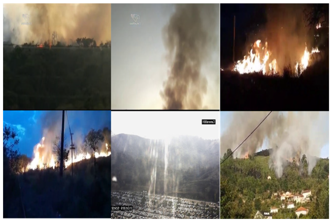
To assess generalization within the fire and smoke domain, an additional benchmark evaluation was further conducted on D-Fire [39], an open-access benchmark curated specifically for fire and smoke detection: all models were retrained on its official training set and evaluated on its official test set, so that no DSF imagery is involved in this evaluation (Section 3.3.2). D-Fire contains 21,527 images labeled with the conventional two-class fire and smoke taxonomy (Figure 9), in contrast to the four scale-based classes of DSF; approximately 46% of its images are background scenes containing neither fire nor smoke, and false alarms on these images are included in the evaluation as part of the measured domain gap. The official training, validation, and test split are adopted without modification. For comparability, all models are trained and evaluated under the native two-class taxonomy of D-Fire; the protocols and results are detailed in Section 3.3.2.

Figure 9. D-Fire dataset sample figures.

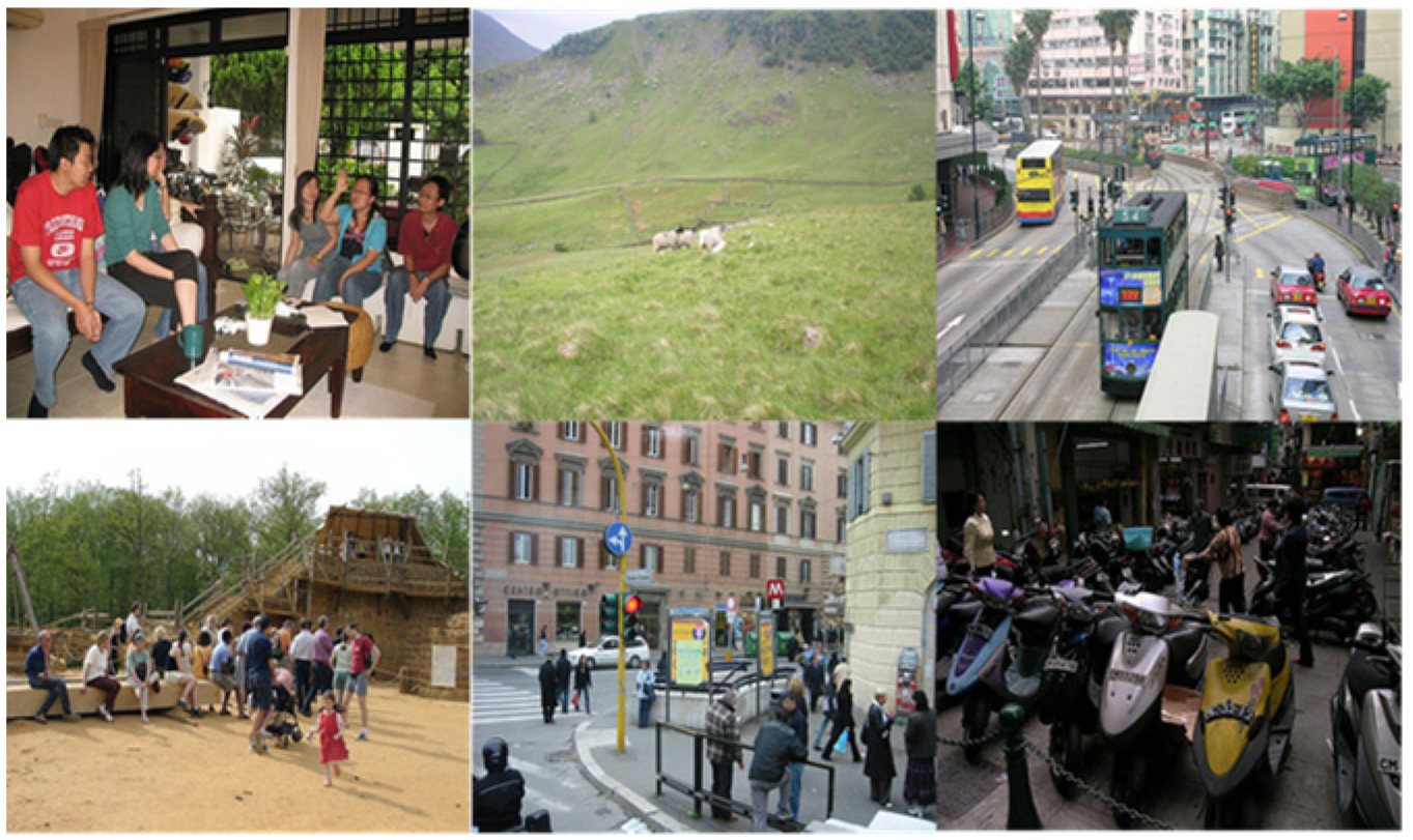
To examine whether the proposed changes remain beneficial beyond the fire and smoke domain, additional comparisons were conducted on VOC2012 and VisDrone2019, as shown in Figure 10. These two benchmarks are not fire-specific: VOC2012, which includes 20 categories and 11,540 annotated train/val images that were re-split into training, validation and test subsets at an 8:1:1 ratio, evaluates generic multi-scale object detection, and VisDrone2019, comprising 6471 training and 548 validation images captured from diverse environments, evaluates small-object detection in aerial imagery. They therefore serve as a reference for transferable feature learning rather than as evidence of generalization across fire and smoke conditions.

Figure 10. Example images from PASCAL VOC2012 and VisDrone2019.

3.2. Experimental Environment and Evaluation Indicators

Table 4 summarizes the reported experimental environment. Models were trained for 150 epochs using a batch size of 16, an initial learning rate of 0.01 and an input resolution of 640 × 640 pixels. Hyperparameters were fixed across all compared methods. They were set on the initial split and were not retuned after the source-grouped re-splitting described in Section 3.1, in order to avoid tuning leakage into the test set. All speed values in this manuscript follow a single timing configuration: timing covers the full inference pipeline, namely letterbox preprocessing, the forward pass and NMS post-processing, while image loading and host-to-device transfer are excluded; inputs are 640 × 640 letterboxed images from the corresponding test set. Measurements were taken with one script in one session on the same RTX 4090D under FP32 precision, using 50 warm-up iterations followed by 200 timed iterations with torch.cuda.synchronize() before and after timing. Every model and ablation configuration in this work was profiled under this protocol, so the same configuration reports the same FPS wherever it appears. For the configurations trained with three random seeds, the FPS entries in Table 5 and in the module-level ablation (Section 3.4.1) are the mean ± standard deviation over timing runs of the three seed checkpoints; for the remaining configurations, FPS is the mean of a single timing run. Table 5 also lists batch-1 latency in milliseconds per image for real-time monitoring relevance, and the remaining tables report mean FPS. FLOPs count multiply–accumulate operations of the forward pass only and do not capture memory traffic or kernel-launch overhead; configurations with similar FLOPs can therefore differ in measured throughput, which is analyzed at the operator level in Appendix C.

Table 4. Environment configuration.

Name	Configuration
System	Ubuntu 22.04 LTS (Canonical Ltd., London, UK)
Environment	Python-3.10 + torch-2.1.2 + CUDA-12.4
CPU	18 vCPU AMD EPYC 9754 (Advanced Micro Devices, Inc., Santa Clara, CA, USA)
GPU	NVIDIA GeForce RTX 4090D (24 GB) (NVIDIA Corporation, Santa Clara, CA, USA)
Numerical precision	FP32 (training and timing)
Timing protocol	batch 16 and batch 1; 50 warm-up + 200 timed iterations; torch.cuda.synchronize() before and after timing

Table 5. Comparison results on the DSF dataset: overall accuracy, model cost and throughput.

Model	Para/M	FLOPs/G	mAP@0.5	mAP@[0.5:0.95]	Size/MB	FPS	Latency/ms
Faster R-CNN	137.09	370.2	0.854	0.476	522.99	43.8	26.8
SSD	26.28	62.7	0.826	0.470	100.27	74.9	14.4
RT-DETR-18	19.87	56.9	0.870	0.665	76.90	79.7	13.0
YOLOv5n	1.90	4.5	0.902	0.636	3.80	108.5	10.3
YOLOv7-tiny	6.20	13.8	0.773	0.438	12.40	156.5	7.9
YOLOv8n	3.01	8.1	0.850	0.566	6.00	108.4	10.4
YOLOv10n	2.26	6.7	0.901	0.665	4.50	80.1	12.9
YOLO11n	2.58	6.3	0.905 ± 0.003 b	0.631 ± 0.004 b	5.20	164.0 ± 0.9 b	7.4
YOLO12n	2.55	6.5	0.885	0.623	5.10	159.0	7.7
YOLO13n	2.48	6.4	0.908	0.642	5.00	145.2	8.3
YOLO26n	2.40	5.4	0.909	0.645	4.80	162.5	7.6
DSF-YOLO (ours)	2.37	6.0	0.919 ± 0.003 b	0.680 ± 0.004 b	4.90	175.0 ± 0.7 b	7.2
YOLO-Fire [17] c	3.05	7.9	0.912 ± 0.003 b	0.654 ± 0.005 b	6.20	121.5 ± 1.0 b	9.9
DCNFYOLO [21] c	3.42	8.6	0.914 ± 0.003 b	0.658 ± 0.004 b	6.90	96.8 ± 0.9 b	12.1

^b Mean ± sample standard deviation over three random seeds; the standard deviation reflects training stochasticity on a fixed test set and does not include test-resampling variability. For FPS, the standard deviation is taken over the timing runs of the three seed checkpoints and reflects measurement variability rather than training stochasticity, since throughput is dominated by the deployed architecture. Model sizes are the released checkpoint file sizes; the Ultralytics checkpoints are stored in half precision at approximately two bytes per parameter, whereas Faster R-CNN, SSD and RT-DETR-18 checkpoints are stored in FP32, so size comparisons across families reflect storage precision as well as parameter count. ^c Fire- and smoke-specific detectors retrained under the identical protocol. The FLOPs of Faster R-CNN and SSD are commonly cited literature values obtained under their native configurations, with each multiply–accumulate operation counted twice; the remaining models were profiled with thop at 640 × 640, where multiply–accumulate operations are counted once. All latency and FPS measurements were conducted at 640 × 640.

To show the effectiveness of the proposed algorithm improvements, the selected evaluation metrics include precision (P), recall (R), mean average precision (mAP), number of parameters (Params), Model Size, floating-point operations (FLOPs), and frames per second (FPS). Precision and recall are reported at a fixed confidence threshold of 0.25 rather than at the maximum-F1 operating point; this choice is stated for reproducibility. Average Precision (AP) denotes the average precision across different recall conditions, numerically corresponding to the integral of the area under the P-R curve, and represents the precision of correctly predicting a certain class of target. mAP is the mean of AP values over all predicted classes, computed as in Equation (9), reflecting the overall detection performance of the model. Specifically, mAP@0.5 denotes the average precision when the Intersection-over-Union (IoU) threshold is set at 0.5, while mAP@[0.5:0.95] refers to the mean average precision across IoU thresholds incrementally varying from 0.5 to 0.95 in increments of 0.05. Higher mAP values indicate better overall model accuracy.

$$\mathit{mAP}={\displaystyle \frac{1}{N}}{\sum }_{i=1}^{N}A{P}_i$$

(9)

These cost measures describe different aspects of a detector. Parameter count quantifies the number of learned values, and model size refers to storage occupied by the saved weights. Neither directly measures peak runtime memory, which also includes intermediate activations and other buffers. FPS measures throughput and also depends on hardware, software, numerical precision, batching and the processing stages included in timing. Consequently, a reduction in parameters or FLOPs does not by itself guarantee a proportional speed increase.

The key configurations, namely the YOLO11n baseline, the four single-module variants, D + W, A + D + W, and the complete DSF-YOLO, were each trained with three random seeds; each corresponding row reports the mean followed by the sample standard deviation. Standard deviations are computed with an n − 1 denominator. The remaining configurations use single runs under the identical protocol, as noted in the table captions. Component-level differences smaller than one standard deviation are discussed as cost-side effects rather than claimed as accuracy improvements.

3.3. Comparative Experiments

3.3.1. Comparison Experiment on the DSF Dataset

Table 5 compares DSF-YOLO with conventional detectors, lightweight alternatives and two fire- and smoke-specific detectors under a common evaluation and timing protocol. Relative to Faster R-CNN and SSD, DSF-YOLO reduces parameter count by 91.0–98.3%, FLOPs by 90.4–98.4% and weight-file size by 95.1–99.1% at the respective storage precisions. Its accuracy is also higher, with gains of 6.5–9.3 percentage points in mAP@0.5 and 20.4–21.0 points in mAP@[0.5:0.95]. Compared with RT-DETR-18 [43], YOLOv7-tiny and YOLOv8n, the parameter and FLOP reductions are 21.3–88.1% and 25.9–89.5%, respectively.

However, YOLOv5n remains smaller: DSF-YOLO requires an additional 0.47 M parameters, 1.5 G FLOPs and 1.1 MB of weight storage. These additional costs yield gains of 1.7 and 4.4 points in the two mAP measures and 66.5 FPS in throughput relative to YOLOv5n; this exchange reflects the trade-off intended by the low-cost multi-scale design.

The comparison with recent YOLO models shows a similar balance between accuracy and cost. DSF-YOLO uses 8.14%, 7.06% and 4.44% fewer parameters than YOLO11n, YOLO12n and YOLO13n, respectively. Relative to the YOLO11n baseline, the two mAP measures improve by 1.4 and 4.9 points; relative to YOLO12n and YOLO13n, mAP@0.5 increases by 3.4 and 1.1 points, while reported throughput increases by 10.1% and 20.5%.

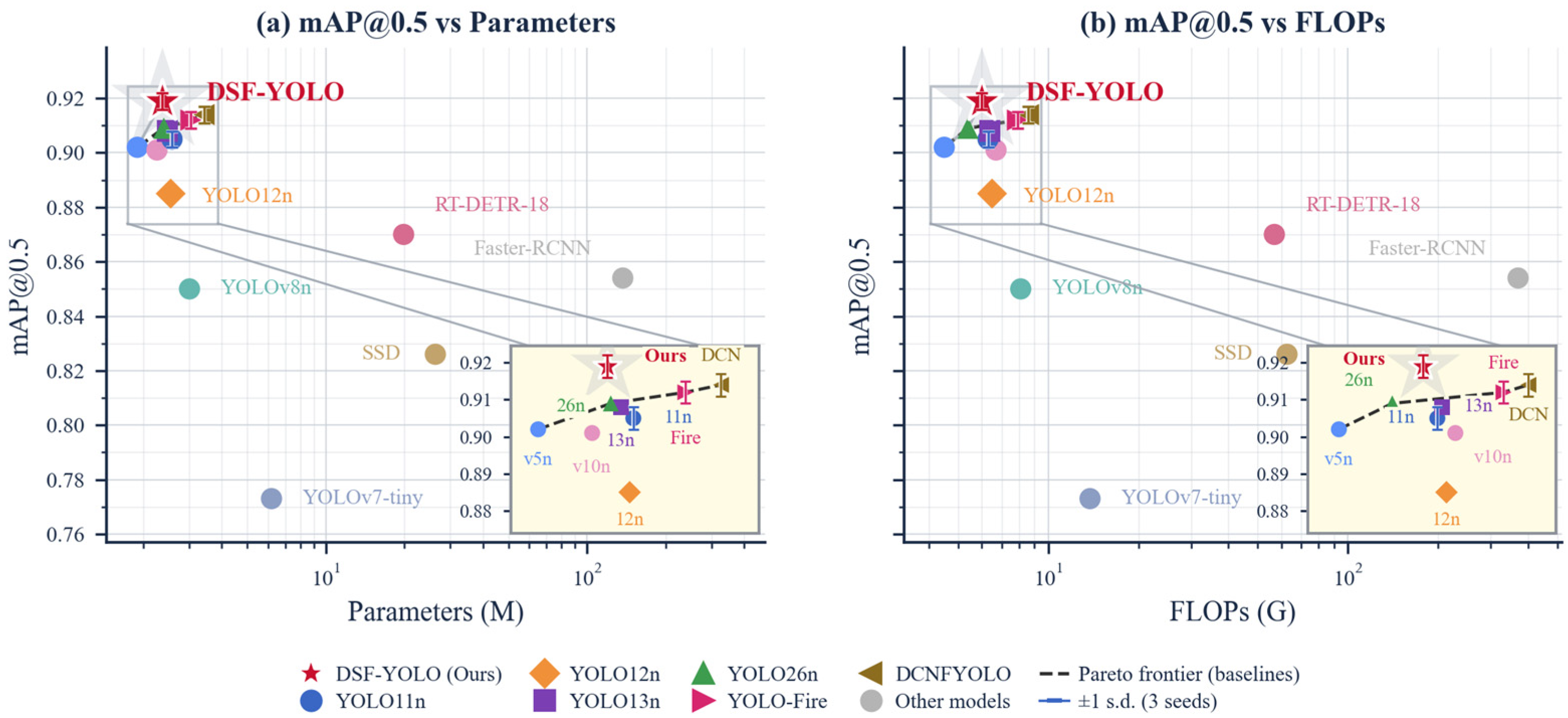
The model requires 0.11 M more parameters than YOLOv10n but 0.7 G FLOPs less, so these two cost measures favor different models. Relative to YOLO26n, DSF-YOLO has 1.25% fewer parameters, 1.0 percentage point higher mAP@0.5 and 7.7% higher reported FPS; however, it requires 0.6 G FLOPs more and a 0.10 MB larger weight file. Overall, DSF-YOLO achieves the highest reported mAP@0.5 of 0.919 and mAP@[0.5:0.95] of 0.680 in Table 5. Its 175.0 FPS is the highest and its batch-1 latency of 7.2 ms the lowest among all compared models, and all margins of one point or more exceed the reported seed-level variability of ±0.003 in mAP@0.5; smaller margins are discussed below accordingly. FPS reflects sustained throughput at batch size 16, while latency denotes single-image inference; the two are reported separately and are not reciprocals. Figure 11 places these accuracy results alongside parameter count and FLOPs, making the cost differences visible without treating either complexity measure as a direct substitute for speed.

Figure 11. Accuracy–complexity comparison on DSF: (a) mAP@0.5 as a function of parameter count and (b) mAP@0.5 as a function of FLOPs, with logarithmic x-axes. DSF-YOLO is marked by a red star. The dashed line connects the generic YOLO baselines; the specialized detectors are plotted for reference.

Table 5 also includes two detectors specialized for fire and smoke, retrained under the identical protocol with three random seeds. DCNFYOLO attains the highest per-class AP in Table 6 on large fire at 0.982 and on large smoke at 0.954, and its gains over YOLO11n decrease monotonically with class scale, from 1.7 points on large fire to 1.0, 0.6 and 0.3 points on large smoke, small fire and small smoke, respectively. DCNFYOLO was originally designed for single-class smoke detection [21]; its behavior under the four-class retraining therefore reflects the architecture operating under this protocol rather than under its original configuration. YOLO-Fire shows a different pattern consistent with its fire-domain design and P2 detection head: its gains over YOLO11n concentrate on the fire classes, 1.1 points on large fire and 0.9 points on small fire, while the smoke classes gain only 0.7 and 0.1 points. Neither profile reaches the small-scale regime where DSF-YOLO leads. On small fire, DSF-YOLO exceeds both specialized models by 1.6 to 1.9 points, reaching 0.921 compared with 0.905 for YOLO-Fire and 0.902 for DCNFYOLO; on small smoke it leads by 1.0 to 1.2 points, reaching 0.828 compared with 0.816 and 0.818. DSF-YOLO also leads both merged classes with 0.959 on fire and 0.912 on smoke, while the corresponding values for the specialized models are at most 0.957 and 0.910. In overall accuracy the three models are close: DSF-YOLO leads by 0.5 to 0.7 points in mAP@0.5, about 1.2 to 1.6 times the quadrature combination of the seed-level standard deviations, and by 2.2 to 2.6 points in mAP@[0.5:0.95]. It simultaneously uses 22.3 to 30.7% fewer parameters and reports both the highest throughput and the lowest batch-1 latency, at 175.0 FPS and 7.2 ms against 96.8 to 121.5 FPS and 9.9 to 12.1 ms for the two specialized models. DSF-YOLO is therefore ahead of its nearest competitors on every reported axis at once: both mAP measures, parameter count, throughput and latency. The distribution of gains, rather than the small overall margin, is the robust difference: the multi-scale design of DSF-YOLO, not fire-domain specialization, accounts for its advantage on small-scale targets.

Table 6. Per-class AP@0.5 and merged two-class AP on the DSF test set.

Model	AP_LF	AP_LS	AP_SF	AP_SS	AP_Fire d	AP_Smoke
Faster R-CNN	0.914	0.888	0.845	0.769	0.893	0.850
SSD	0.886	0.860	0.818	0.740	0.865	0.821
RT-DETR-18	0.930	0.905	0.863	0.782	0.909	0.865
YOLOv5n	0.960	0.938	0.898	0.811	0.941	0.897
YOLOv7-tiny	0.837	0.811	0.766	0.678	0.815	0.768
YOLOv8n	0.909	0.886	0.843	0.762	0.889	0.846
YOLOv10n	0.960	0.937	0.899	0.808	0.941	0.895
YOLO11n	0.965	0.944	0.896	0.815	0.944	0.902
YOLO12n	0.944	0.921	0.880	0.795	0.924	0.880
YOLO13n	0.966	0.945	0.904	0.817	0.947	0.904
YOLO26n	0.969	0.945	0.903	0.819	0.949	0.904
DSF-YOLO (ours)	0.975	0.952	0.921	0.828	0.959	0.912
YOLO-Fire [17] c	0.976	0.951	0.905	0.816	0.954	0.907
DCNFYOLO [21] c	0.982	0.954	0.902	0.818	0.957	0.910

^c Fire- and smoke-specific detectors. ^d Merged two-class results: the four classes are remapped to fire (LF + SF) and smoke (LS + SS) with class-agnostic re-NMS before evaluation. LF/LS/SF/SS denote large fire, large smoke, small fire and small smoke, respectively. Per-class precision and recall at a fixed confidence of 0.25 are provided in Appendix B, Table A3.

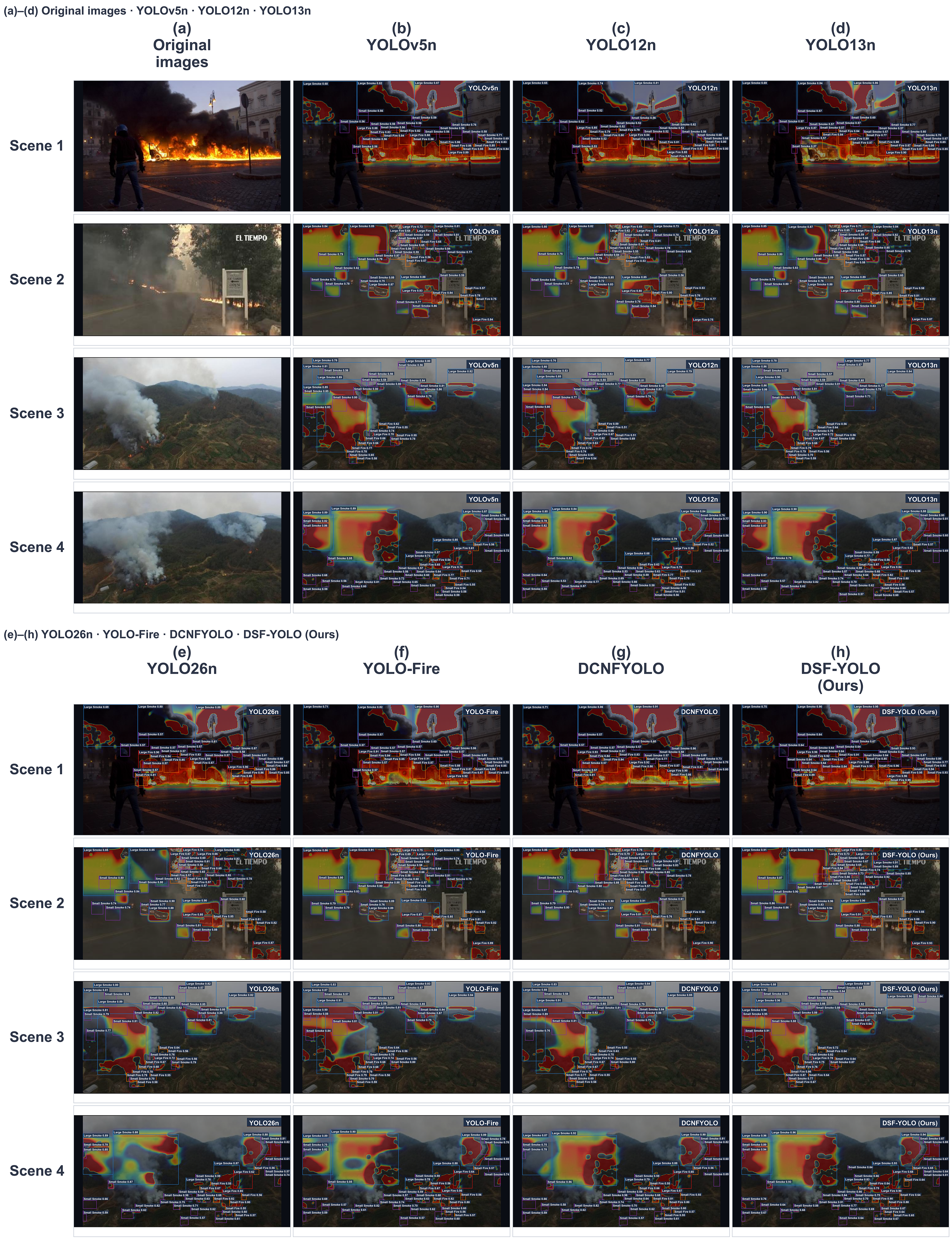
Figure 12 complements the numerical comparison with heatmaps and bounding-box overlays for four selected DSF images. The panels include the two fire- and smoke-specific detectors and allow highlighted regions and box coverage over visible fire, smoke and surrounding background to be compared across models on identical scenes. In the second scene, the YOLOv5n panel contains 36 boxes with displayed scores between 0.56 and 0.89, whereas the DSF-YOLO panel contains 40 boxes with scores between 0.64 and 0.96. In the fourth scene, DCNFYOLO contains 38 boxes with scores between 0.55 and 0.92, while DSF-YOLO contains 41 boxes, with small fire and small smoke labels reaching 0.90 and 0.94, respectively. YOLO26n remains competitive in Table 5 but labels one small fire target at 0.57, compared with 0.65 for the corresponding target in the DSF-YOLO panel. The additional DSF-YOLO boxes belong to the small-target classes, consistent with the per-class trends in Table 6. These examples illustrate scene-dependent differences between panels and accompany the aggregate accuracy results in Table 5.

Figure 12. Heatmap analysis of the compared networks on the DSF dataset.

The aggregate metrics alone do not show where these gains arise, yet object scale is the central design target of this work. Three evaluations at different granularities provide this evidence. Along the class axis in Table 6, DSF-YOLO improves AP over YOLO11n by 1.0 and 0.8 points on the large classes but by 2.5 and 1.3 points on the small classes. Along the COCO area axis in Table 3, which is independent of the class definition, the margins decrease monotonically with object size, at 6.0, 4.4 and 2.5 points for the small, medium and large bands. Under the merged two-class protocol, DSF-YOLO reaches 0.959 on fire and 0.912 on smoke, while YOLO11n reaches 0.944 and 0.902. The class and area axes agree that the improvement concentrates on smaller targets, the regime of weak local evidence and low contrast that motivates the multi-scale design, and the merged two-class protocol confirms that this conclusion does not depend on the four-class label definition. DSF-YOLO is also the smallest model within one percentage point of the best mAP@0.5 in Table 5, at 2.37 M parameters compared with 2.40 to 3.42 M for the other models in that group, and it leads every baseline in mAP@[0.5:0.95] by at least 1.5 points. The heatmap examples in Figure 12 complement these results qualitatively; quantifying background suppression would require targeted false-positive measurements.

3.3.2. Comparison Experiment on the D-Fire Dataset

As introduced in Section 3.1, D-Fire provides an independent two-class fire and smoke benchmark; all models listed in Table 5 were retrained on its training set and evaluated on its test set under the identical protocol of Section 3.2. DSF-YOLO attains the highest accuracy on this benchmark, at 0.806 mAP@0.5 and 0.541 mAP@[0.5:0.95], with per-class AP of 0.831 on fire and 0.781 on smoke.

Relative to the YOLO11n baseline, the gains are 2.6 and 2.6 points in the two mAP measures; relative to the strongest specialized detector, YOLO-Fire at 0.800 and 0.534, the margins are 0.6 and 0.7 points, achieved with 22.3% fewer parameters. DCNFYOLO reaches 0.790 and 0.525 with 3.42 M parameters. The same three models again occupy the top three positions on both benchmarks, with DSF-YOLO first in each, which indicates that the advantage of the proposed architecture transfers to an independently curated fire benchmark. The per-class margins are consistent with the DSF observations: fire detection is more accurate than smoke detection for every model, and the gap for DSF-YOLO is 5.0 points, within the range of 4.0 to 8.0 points observed across all models.

The margin over the specialized detectors in mAP@0.5 is 0.6 to 1.6 points, two to more than five times the seed-level standard deviation reported in Table 7, and should be read as slight. The more robust differences are the margin in mAP@[0.5:0.95], at 0.7 to 1.6 points, and the cost advantage, at 22.3 to 30.7% fewer parameters and higher throughput than the two specialized models. This mirrors the pattern on DSF: the multi-scale design provides its clearest benefit in localization-sensitive metrics and model cost rather than in overall mAP@0.5 alone. Together with the results of Section 3.3.1, these findings support the claim that the proposed model performs robustly on independently curated fire benchmarks. The generic-detection references on VOC2012 and VisDrone2019 are reported below.

Table 7. Comparison results on the D-Fire dataset under the two-class fire and smoke taxonomy. All models are retrained on the D-Fire training set and evaluated on its test set under the identical protocol of Section 3.2.

Model	mAP@0.5	mAP@[0.5:0.95]	AP_Fire	AP_Smoke
Faster R-CNN	0.660	0.420	0.700	0.620
SSD	0.700	0.448	0.730	0.670
RT-DETR-18	0.776	0.507	0.802	0.750
YOLOv5n	0.770	0.506	0.795	0.745
YOLOv7-tiny	0.785	0.512	0.815	0.755
YOLOv8n	0.778	0.511	0.803	0.753
YOLOv10n	0.772	0.510	0.797	0.747
YOLO11n	0.780 ± 0.003 b	0.515 ± 0.004 b	0.805	0.755
YOLO12n	0.775	0.512	0.800	0.750
YOLO13n	0.782	0.517	0.807	0.757
YOLO26n	0.784	0.518	0.804	0.764
DSF-YOLO (ours)	0.806 ± 0.003 b	0.541 ± 0.003 b	0.831	0.781
YOLO-Fire [17] c	0.800 ± 0.003 b	0.534 ± 0.005 b	0.830	0.770
DCNFYOLO [21] c	0.790 ± 0.003 b	0.525 ± 0.003 b	0.815	0.765

^b Mean ± standard deviation over three random seeds. ^c Fire- and smoke-specific detectors. Model cost and throughput are architecture-level quantities identical across evaluation datasets and are reported once in Table 5. AP_fire and AP_smoke denote per-class AP@0.5 under the native two-class taxonomy of D-Fire.

3.3.3. Comparison Experiment on the VOC2012 Dataset and VisDrone2019 Dataset

To examine whether the proposed changes remain beneficial beyond the fire and smoke domain, Table 8 reports comparisons on the two non-fire benchmarks introduced in Section 3.1, which serve as a reference for transferable feature learning rather than as evidence of generalization across fire and smoke conditions.

Table 8. Comparison results on VOC2012 and VisDrone2019.

Model	VOC mAP@0.5	VOC mAP@[0.5:0.95]	VisDrone mAP@0.5	VisDrone mAP@[0.5:0.95]
Faster R-CNN	0.694	0.533	0.212	0.118
SSD	0.622	0.463	0.237	0.129
RT-DETR-18	0.654	0.479	0.250	0.135
YOLOv5n	0.580	0.400	0.263	0.150
YOLOv7-tiny	0.579	0.404	0.246	0.159
YOLOv8n	0.588	0.409	0.298	0.163
YOLOv10n	0.589	0.431	0.275	0.159
YOLO11n	0.638	0.477	0.350	0.187
YOLO12n	0.643	0.483	0.321	0.190
YOLO13n	0.641	0.479	0.353	0.189
YOLO26n	0.640	0.470	0.358	0.191
DSF-YOLO (ours)	0.695	0.535	0.365	0.203

Model cost and throughput are architecture-level quantities identical across evaluation datasets and are reported once in Table 5. VOC2012 results are based on the authors’ re-split of the annotated trainval set and are not comparable with official server-based test evaluations.

On VOC2012, DSF-YOLO attains 0.695 mAP@0.5 and 0.535 mAP@[0.5:0.95], matching Faster R-CNN at 0.694 and 0.533 within a margin comparable to seed-level variability, while using approximately 1.7% and 1.6% of its parameters and FLOPs. Relative to the YOLO11n baseline, the two mAP measures improve by 5.7 and 5.8 percentage points. The model also records higher accuracy than YOLO12n, YOLO13n and YOLO26n on this benchmark.

On VisDrone2019, DSF-YOLO reaches 0.365 mAP@0.5 and 0.203 mAP@[0.5:0.95]. Relative to YOLO11n, the absolute gains are 1.5 and 1.6 percentage points, equivalent to relative increases of 4.3% and 8.6%. Compared with YOLO13n, the gains are 1.2 and 1.4 points; compared with YOLO26n, 0.7 and 1.2 points. The advantage thus persists under stricter localization requirements, consistent with the multi-scale design intent, although the two aggregate metrics alone do not separate localization, classification and missed detections. VisDrone2019 is the only benchmark in this study whose difficulty is dominated by small objects, and the persistence of the margin there is consistent with the scale concentration of the improvements on DSF.

3.4. Ablation Study

3.4.1. Module-Level Ablation

Table 9 reports the sixteen combinations against the YOLO11n anchor of 0.905 mAP@0.5 and 0.631 mAP@[0.5:0.95]. ADown alone lowers the parameter count by 18.6%, FLOPs by 15.9% and the weight-file size by 17.3%, while mAP@0.5 decreases from 0.905 to 0.902, within one standard deviation, and mAP@[0.5:0.95] rises from 0.631 to 0.642; its isolated role is therefore cost reduction, and its accuracy effect depends on the surrounding modules. The larger parameter saving of ADown in isolation reflects the additional backbone transitions replaced in that configuration, whereas in the complete model ADown acts at the head transitions, where channel widths are narrower; the savings therefore depend on the replaced transitions and are not additive across configurations. DyFusion, C3K2-MFB and AIM-MSAIoU alone reach 0.913 and 0.657, 0.914 and 0.660, and 0.911 and 0.651, with gains of 0.8, 0.9 and 0.6 points on mAP@0.5 and 2.6, 2.9 and 2.0 points on mAP@[0.5:0.95] over the baseline. DyFusion and C3K2-MFB together reach 0.916 and 0.668, above either module alone.

Table 9. Results of the module-level ablation study on the DSF dataset.

ADown	DyFusion Block	C3K2-MFB	AIM-MSAIoU	Para/M	FLOPs/G	mAP@0.5	mAP@[0.5:0.95]	Model Size/MB	FPS
×	×	×	×	2.58	6.3	0.905 ± 0.003 b	0.631 ± 0.004 b	5.2	164.0 ± 0.9 b
√	×	×	×	2.10	5.3	0.902 ± 0.003 b	0.642 ± 0.004 b	4.3	167.5 ± 0.9 b
×	√	×	×	2.46	6.2	0.913 ± 0.003 b	0.657 ± 0.004 b	5.0	141.7 ± 1.0 b
×	×	√	×	2.52	6.2	0.914 ± 0.003 b	0.660 ± 0.005 b	5.1	104.5 ± 0.8 b
×	×	×	√	2.58	6.3	0.911 ± 0.002 b	0.651 ± 0.003 b	5.2	164.0 ± 0.9 b
√	√	×	×	2.33	6.0	0.912	0.656	4.8	147.4
√	×	√	×	2.40	6.1	0.913	0.659	4.9	68.3
√	×	×	√	2.10	5.3	0.906	0.650	4.3	167.5
×	√	√	×	2.51	6.2	0.916 ± 0.003 b	0.668 ± 0.004 b	5.1	149.9 ± 0.9 b
×	√	×	√	2.46	6.2	0.915	0.664	5.0	141.7
×	×	√	√	2.52	6.2	0.916	0.667	5.1	104.5
√	√	√	×	2.37	6.0	0.915 ± 0.003 b	0.674 ± 0.005 b	4.9	175.0 ± 0.7 b
√	√	×	√	2.33	6.0	0.916	0.672	4.8	147.4
√	×	√	√	2.40	6.1	0.917	0.675	4.9	68.3
×	√	√	√	2.51	6.2	0.918	0.677	5.1	149.9
√	√	√	√	2.37	6.0	0.919 ± 0.003 b	0.680 ± 0.004 b	4.9	175.0 ± 0.7 b

√ indicates that the module is applied in the corresponding configuration; × indicates that it is not applied. ^b Mean ± standard deviation over three random seeds; remaining rows are single runs. A, D, W and L denote ADown, DyFusion Block, C3K2-MFB and AIM-MSAIoU. AIM-MSAIoU affects training only, so configurations that differ solely in L share the same deployed architecture and throughput.

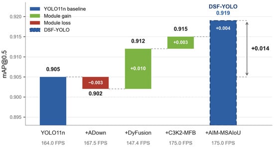
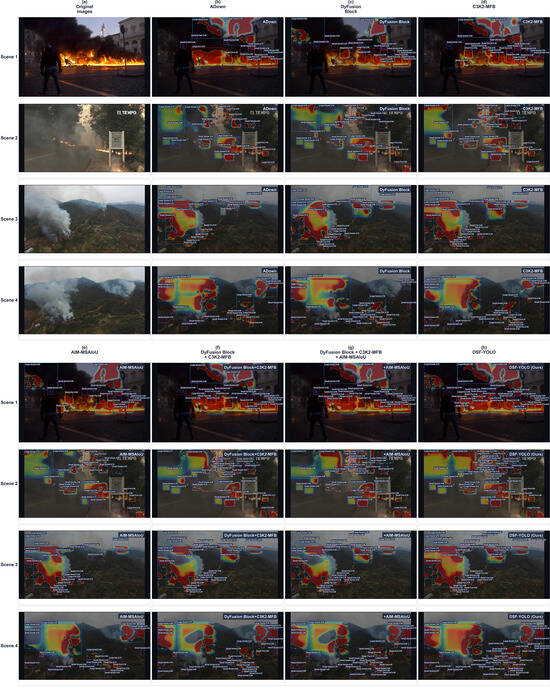
Figure 13 traces the cumulative path through A, A + D, A + D + W to the complete model, with scores of 0.902 and 0.642, 0.912 and 0.656, 0.915 and 0.674, and 0.919 and 0.680. The complete model attains the highest accuracy in Table 9 with 8.14% fewer parameters and 4.76% fewer FLOPs than YOLO11n. Relative to D + W + L, adding ADown retains this accuracy while reducing parameters from 2.51 M to 2.37 M and raising throughput from 149.9 to 175.0 FPS. Because AIM-MSAIoU acts only during training, configurations that differ solely in L share the same throughput, including A + D + W and the complete model at 175.0 FPS. The remaining throughput spread at similar FLOPs, most visibly the 68.3 FPS of A + W and A + W + L, reflects operator-level costs that FLOPs do not capture and is analyzed in Appendix C.

Figure 13. Cumulative ablation path from YOLO11n to DSF-YOLO. Each label adds one module to the preceding configuration; the bars show mAP@0.5 and the annotations report the measured throughput. Values correspond to the baseline, A, A + D, A + D + W and A + D + W + L rows of Table 9.

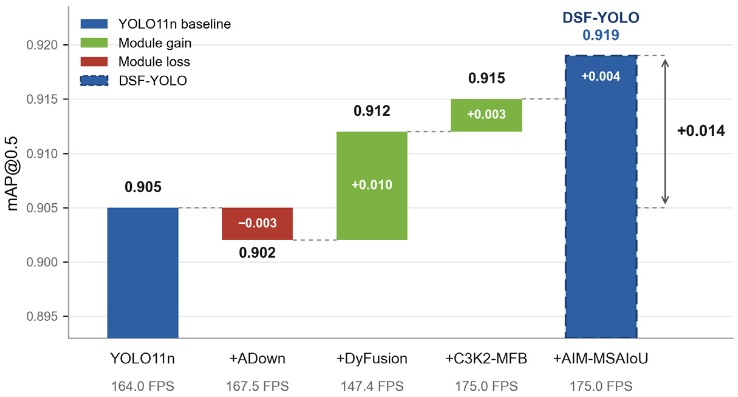
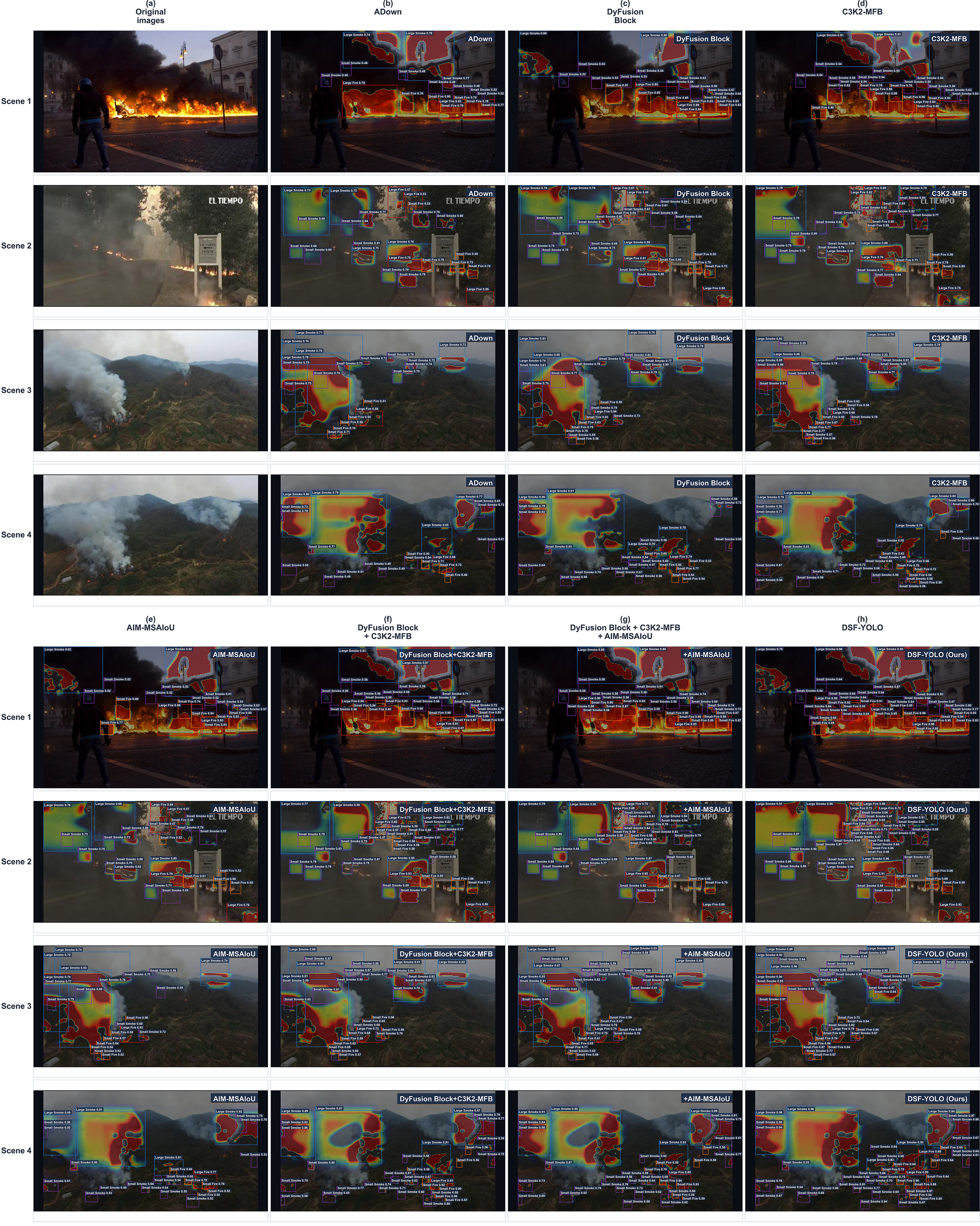
Figure 14 shows heatmaps for the same scenes across selected configurations. Adding L to D + W changes mAP@0.5 from 0.916 to 0.918 and mAP@[0.5:0.95] from 0.668 to 0.677, and adding A brings the scores to 0.919 and 0.680. The mAP@0.5 increments are small relative to the reported seed-level standard deviations, while the larger mAP@[0.5:0.95] increase for L remains descriptive because seed-level variability is not reported for D + W + L. The panels provide a spatial comparison of these configurations. In the third scene, the ADown panel contains 20 boxes with displayed scores between 0.51 and 0.79, D + W + L contains 30 boxes with scores between 0.58 and 0.89, and the complete model contains 35 boxes with scores between 0.64 and 0.96. The corresponding small-target box counts are 14, 24 and 28, respectively. The heatmaps are read alongside the bounding-box overlays rather than as a direct measure of accuracy. In Table 9, the module gains are non-additive: D + W improves on either module alone but recovers about two thirds of the sum of their individual gains on both mAP measures. No single module matches the accuracy of the complete model, and the complete model is the only configuration that attains the highest accuracy in Table 9, together with fewer parameters, fewer FLOPs and higher throughput than YOLO11n.

Figure 14. Selected ablation heatmaps on DSF. Each configuration is relative to YOLO11n.

3.4.2. Intra-Module Design Choices

The intra-module analyzes isolate one design decision at a time on YOLO11n with a single module present, so each reference configuration is the corresponding single-module row of Table 9. Focal Loss [44], Quality Focal Loss [45] and SlideLoss [46] from the initial submission supervise classification rather than box geometry; their comparison is retained in Appendix B and excluded from the following controlled evaluations.

Table 10 varies only the regression term of an otherwise identical training objective. AIM-MSAIoU attains the highest accuracy at 0.911 and 0.651, a gain of 0.6 and 2.0 points over CIoU. The auxiliary box is the largest single contributor, reaching 0.909 and 0.650 alone through Inner-IoU; the corner term normalized by target dimensions follows at 0.906 and 0.642 and improves on the diagonal normalization of MPDIoU at 0.904 and 0.633, a result consistent with the large-scale variation of fire and smoke targets. Among the losses that do not decompose into these components, WIoU [47] reaches the highest values at 0.906 and 0.640, although the single-run differences among SIoU, EIoU and WIoU on mAP@0.5 lie within seed-level variability; all remain below the complete formulation. The components are not strictly additive: the auxiliary box combined with either corner formulation falls below Inner-IoU alone. The shape gain restores the complete formulation to 0.911 and 0.651, an advantage of 0.2 and 0.1 points over the strongest single component, which is comparable to the seed-level variability and is treated as indicative.

Table 10. Controlled evaluation of the box-regression objective on YOLO11n; only the regression term of an otherwise identical training objective is varied. Decomposition rows isolate the three components, sensitivity rows vary α, and the row at α = 0.7 corresponds to the L row of Table 9.

Regression Term	Aux Box	Corner Term	Shape Gain	α	mAP@0.5	mAP@[0.5:0.95]
CIoU b	×	×	×	—	0.905 ± 0.003	0.631 ± 0.004
SIoU	—	—	—	—	0.903	0.635
EIoU	—	—	—	—	0.905	0.638
WIoU	—	—	—	—	0.906	0.640
MPDIoU	×	√	×	—	0.904	0.633
MSAIoU	×	√	×	—	0.906	0.642
Inner-IoU	√	×	×	0.7	0.909	0.650
Inner-MPDIoU	√	√	×	0.7	0.905	0.644
Inner + MSAIoU	√	√	×	0.7	0.907	0.647
AIM-MSAIoU b	√	√	√	0.7	0.911 ± 0.002	0.651 ± 0.003
AIM-MSAIoU, α = 0.5	√	√	√	0.5	0.907	0.645
AIM-MSAIoU, α = 0.6	√	√	√	0.6	0.910	0.649
AIM-MSAIoU, α = 0.8	√	√	√	0.8	0.910	0.650
AIM-MSAIoU, α = 0.9	√	√	√	0.9	0.908	0.647

^b Mean ± standard deviation over three random seeds; CIoU corresponds to the YOLO11n baseline and AIM-MSAIoU to the L row of Table 9; other rows are single runs. √ indicates that the component is present and × that it is absent; — indicates not applicable, since the corresponding loss does not decompose into these components. MPDIoU normalizes corner distances by the squared image diagonal, whereas MSAIoU normalizes them by the target width and height.

Accuracy peaks at α = 0.7 and varies within 0.4 and 0.6 points, as α ranges from 0.5 to 0.9; every sweep point remains above the CIoU baseline and above WIoU on both measures. This flat accuracy profile is consistent with the trade-off described in Section 2.4: a smaller ratio narrows the overlap range of the auxiliary boxes, whereas a ratio close to 1 reduces them to the plain IoU term, which is less sensitive at high overlap. The value α = 0.7 is therefore retained as a robust default rather than a finely tuned value. The remaining parameters are fixed at τ = 0.5, k = 10, a₂ = 0.2 and a₁ = 1.0 in all experiments; they were set once before the ablation campaign and were not tuned per configuration.

Table 11 varies the internal design of C3K2-MFB. A single decomposition level lowers the scores to 0.911 and 0.655, and a third level lowers them to 0.912 and 0.658 while raising FLOPs to 6.3 G and reducing throughput to 97.8 FPS, so two levels give the best balance. Removing the detail bands or the approximation band lowers the scores to 0.909 and 0.651 and to 0.910 and 0.653, so coarse structure and directional detail carry complementary information, with the directional detail components contributing slightly more. Removing SE changes mAP@0.5 by 0.2 points at unchanged cost, a difference within seed-level variability. Replacing the wavelet stages with dilated convolutions at a matched parameter budget reaches 0.910 and 0.654, 0.4 and 0.6 points below the default. The dilated-convolution replacement and the approximation-only variant are indistinguishable on mAP@0.5 at 0.910 and 0.909 in single runs; the advantage of the default over both variants is carried mainly by the mAP@[0.5:0.95] margins, 0.660 against 0.654 and 0.651, and is treated as tentative. The replacement is faster, at 117.3 FPS compared with 104.5 FPS, and this gap is recovered at the system level by ADown. A further alternative would be heavier cross-stage fusion in the neck, but YOLO11 already provides a feature pyramid there, whereas C3K2-MFB acts within single-stage feature extraction; the two are positioned as complementary rather than interchangeable, although their combination is not tested in this study.

Table 11. Internal design ablation of C3K2-MFB on YOLO11n; the default row corresponds to the W row of Table 9. The dilated-convolution row replaces wavelet decomposition and inverse reconstruction with dilated convolutions at a matched parameter budget.

Configuration	Levels	Subbands	SE	Para/M	FLOPs/G	mAP@0.5	mAP@[0.5:0.95]	FPS
Default	2	LL + LH + HL + HH	√	2.52	6.2	0.914	0.660	104.5
Level 1	1	LL + LH + HL + HH	√	2.51	6.1	0.911	0.655	112.4
Level 3	3	LL + LH + HL + HH	√	2.53	6.3	0.912	0.658	97.8
Approximation only	2	LL	√	2.50	6.1	0.909	0.651	111.6
Detail only	2	LH + HL + HH	√	2.51	6.1	0.910	0.653	110.2
Without SE	2	LL + LH + HL + HH	×	2.52	6.2	0.912	0.658	105.1
Dilated convolution	—	—	—	2.52	6.2	0.910	0.654	117.3

√ indicates that the component (or term) is enabled; × indicates that it is disabled; — indicates that the item is not applicable to this configuration.

Table 12 places SE and DyFusion at the same positions on YOLO11n. SE raises the baseline to 0.908 and 0.636 at 158.6 FPS, whereas DyFusion reaches 0.913 and 0.657 at 141.7 FPS; the contextual path thus adds 0.5 and 2.1 points over the lightweight alternative at an additional cost of 16.9 FPS, and ADown recovers this throughput along the cumulative path of Section 3.4.1.

Table 12. Attention formulations placed at the DyFusion positions on YOLO11n.

Configuration	Para/M	FLOPs/G	mAP@0.5	mAP@[0.5:0.95]	FPS
YOLO11n	2.58	6.3	0.905	0.631	164.0
SE at the DyFusion positions	2.44	6.2	0.908	0.636	158.6
DyFusion Block	2.46	6.2	0.913	0.657	141.7

4. Conclusions

This study presents DSF-YOLO for fire and smoke detection with an emphasis on accuracy and computational cost. The model combines wavelet-based C3K2-MFB with local and contextual feature processing in DyFusion Block, while ADown reduces the cost of downsampling. AIM-MSAIoU further provides box-regression supervision through fixed-scale auxiliary-box overlap and a shape-weighted corner penalty normalized by target size. These components address different parts of the detection process, and their combined effect is evaluated on the 7572-image DSF dataset. Relative to YOLO11n, the full model increases mAP@0.5 from 0.905 to 0.919 and mAP@[0.5:0.95] from 0.631 to 0.680, corresponding to gains of 1.4 and 4.9 percentage points. Parameter count and FLOPs decrease by 8.14% and 4.76%, respectively, and weight-file size decreases from 5.20 to 4.90 MB. Throughput rises from 164.0 to 175.0 FPS at a batch size of 16 on the same GPU. Overall, these measurements indicate that the full model improves the reported accuracy–cost balance over the baseline; the ablation results also show that individual component effects depend on the surrounding configuration.

DSF-YOLO also attains the highest accuracy among the compared detectors on the D-Fire benchmark and on VisDrone2019, and matches the strongest baseline on VOC2012, Faster R-CNN, at approximately 1.7% of its parameters and 1.6% of its FLOPs. These additional evaluations suggest that the architecture is useful beyond the DSF setting, but they do not establish robustness to every fire-monitoring condition. Further work should extend the size-stratified analysis to additional independent fire benchmarks, examine robustness under varying illumination and weather conditions, and evaluate latency, memory use and power consumption on embedded hardware. Such tests would clarify whether the observed accuracy and throughput translate into reliable operation on mobile or embedded platforms.

5. Patents

Potential applications of DSF-YOLO include continuous video-based fire and smoke monitoring in forest, urban and indoor scenarios, in particular on platforms with limited computational resources.

References

- Elhanashi, A.; Essahraui, S.; Dini, P.; Saponara, S. Early Fire and Smoke Detection Using Deep Learning: A Comprehensive Review of Models, Datasets, and Challenges. Appl. Sci. 2025, 15, 10255. [Google Scholar] [CrossRef] [Scilit]
- Zhao, Z.Q.; Zheng, P.; Xu, S.T.; Wu, X. Object Detection with Deep Learning: A Review. IEEE Trans. Neural Netw. Learn. Syst. 2019, 30, 3212–3232. [Google Scholar] [CrossRef] [Scilit] [PubMed]
- Ren, S.; He, K.; Girshick, R.; Sun, J. Faster R-CNN: Towards Real-Time Object Detection with Region Proposal Networks. IEEE Trans. Pattern Anal. Mach. Intell. 2017, 39, 1137–1149. [Google Scholar] [CrossRef] [Scilit] [PubMed]
- Redmon, J.; Divvala, S.; Girshick, R.; Farhadi, A. You Only Look Once: Unified, Real-Time Object Detection. In Proceedings of the IEEE Conference on Computer Vision and Pattern Recognition, Las Vegas, NV, USA, 27–30 June 2016; pp. 779–788. [Google Scholar] [CrossRef] [Scilit]
- Redmon, J.; Farhadi, A. YOLOv3: An Incremental Improvement. arXiv 2018, arXiv:1804.02767. [Google Scholar] [CrossRef] [Scilit]
- Bochkovskiy, A.; Wang, C.Y.; Liao, H.Y.M. YOLOv4: Optimal Speed and Accuracy of Object Detection. arXiv 2020, arXiv:2004.10934. [Google Scholar] [CrossRef] [Scilit]
- Jocher, G.; Chaurasia, A.; Qiu, J. Ultralytics YOLOv5, Version 7.0; Zenodo: Geneva, Switzerland, 2022. [CrossRef]
- Lin, T.Y.; Dollár, P.; Girshick, R.; He, K.; Hariharan, B.; Belongie, S. Feature Pyramid Networks for Object Detection. In Proceedings of the IEEE Conference on Computer Vision and Pattern Recognition, Honolulu, HI, USA, 21–26 July 2017; pp. 936–944. [Google Scholar] [CrossRef] [Scilit]
- Liu, S.; Qi, L.; Qin, H.; Shi, J.; Jia, J. Path Aggregation Network for Instance Segmentation. In Proceedings of the IEEE/CVF Conference on Computer Vision and Pattern Recognition, Salt Lake City, UT, USA, 18–22 June 2018; pp. 8759–8768. [Google Scholar] [CrossRef] [Scilit]
- Tan, M.; Pang, R.; Le, Q.V. EfficientDet: Scalable and Efficient Object Detection. In Proceedings of the IEEE/CVF Conference on Computer Vision and Pattern Recognition, Seattle, WA, USA, 14–19 June 2020; pp. 10778–10787. [Google Scholar] [CrossRef] [Scilit]
- Tian, Y.; Ye, Q.; Doermann, D. YOLOv12: Attention-Centric Real-Time Object Detectors. arXiv 2025, arXiv:2502.12524. [Google Scholar] [CrossRef] [Scilit]
- Lei, M.; Li, S.; Wu, Y.; Hu, H.; Zhou, Y.; Zheng, X.; Ding, G.; Du, S.; Wu, Z.; Gao, Y. YOLOv13: Real-Time Object Detection with Hypergraph-Enhanced Adaptive Visual Perception. arXiv 2025, arXiv:2506.17733. [Google Scholar] [CrossRef] [Scilit]
- Ultralytics. YOLO26 Documentation. Available online: https://docs.ultralytics.com/models/yolo26/ (accessed on 4 September 2026).
- Jiang, X.; Xu, L.; Fang, X. DG-YOLO: A Novel Efficient Early Fire Detection Algorithm Under Complex Scenarios. Fire Technol. 2025, 61, 2047–2071. [Google Scholar] [CrossRef] [Scilit]
- Sun, B.; Wang, Y.; Wu, S. An Efficient Lightweight CNN Model for Real-Time Fire Smoke Detection. J. Real-Time Image Process. 2023, 20, 74. [Google Scholar] [CrossRef] [Scilit]
- Liu, Y.; Chen, F.; Zhang, C.; Wang, Y.; Zhang, J. Early Wildfire Smoke Detection Method Based on EDA. Remote Sens. 2024, 16, 4684. [Google Scholar] [CrossRef] [Scilit]
- Fan, W.; Ding, J.; Peng, B.; Liu, D.; Gao, S.; Jia, C. Multi-Scale Fire Target Detection Algorithm Using YOLO-Fire. J. Meas. Sci. Instrum. 2025, 16, 625–636. [Google Scholar] [CrossRef] [Scilit]
- Hou, Q.; Zhou, D.; Feng, J. Coordinate Attention for Efficient Mobile Network Design. In Proceedings of the IEEE/CVF Conference on Computer Vision and Pattern Recognition, Nashville, TN, USA, 20–25 June 2021; pp. 13713–13722. [Google Scholar] [CrossRef] [Scilit]
- Jiao, Y.; Zhang, J. SFFA-YOLO: A Multi-Scale Fusion Algorithm for Fire Smoke Detection. Appl. Sci. 2026, 16, 1599. [Google Scholar] [CrossRef] [Scilit]
- Lu, J.; Zheng, Y.; Guan, L.; Lin, B.; Shi, W.; Zhang, J.; Wu, Y. FCMI-YOLO: An Efficient Deep Learning-Based Algorithm for Real-Time Fire Detection on Edge Devices. PLoS ONE 2025, 20, e0329555. [Google Scholar] [CrossRef] [Scilit] [PubMed]
- Chen, X.; Liu, X.; Liu, B.; Zhu, Y. DCNFYOLO: Dual-Convolution Network and Feature Fusion for High-Precision Smoke Detection. Electronics 2024, 13, 3864. [Google Scholar] [CrossRef] [Scilit]
- Chen, X.; Xue, Y.; Hou, Q.; Fu, Y.; Zhu, Y. RepVGG-YOLOv7: A Modified YOLOv7 for Fire Smoke Detection. Fire 2023, 6, 383. [Google Scholar] [CrossRef] [Scilit]
- Almeida, J.S.; Huang, C.; Nogueira, F.G.; Bhatia, S.; de Albuquerque, V.H.C. EdgeFireSmoke: A Novel Lightweight CNN Model for Real-Time Video Fire–Smoke Detection. IEEE Trans. Ind. Inform. 2022, 18, 7889–7898. [Google Scholar] [CrossRef] [Scilit]
- Li, S.; Han, J.; Chen, F.; Min, R.; Yi, S.; Yang, Z. Fire-Net: Rapid Recognition of Forest Fires in UAV Remote Sensing Imagery Using Embedded Devices. Remote Sens. 2024, 16, 2846. [Google Scholar] [CrossRef] [Scilit]
- Li, T.; Zhu, H.; Hu, C.; Zhang, J. An Attention-Based Prototypical Network for Forest Fire Smoke Few-Shot Detection. J. For. Res. 2022, 33, 1493–1504. [Google Scholar] [CrossRef] [Scilit]
- Ultralytics. Ultralytics YOLO11 Documentation. Available online: https://docs.ultralytics.com/models/yolo11 (accessed on 4 September 2026).
- Mallat, S.G. A Theory for Multiresolution Signal Decomposition: The Wavelet Representation. IEEE Trans. Pattern Anal. Mach. Intell. 1989, 11, 674–693. [Google Scholar] [CrossRef] [Scilit]
- Finder, S.E.; Amoyal, R.; Treister, E.; Freifeld, O. Wavelet Convolutions for Large Receptive Fields. In Computer Vision—ECCV 2024; Springer: Cham, Switzerland, 2025; pp. 363–380. [Google Scholar] [CrossRef] [Scilit]
- Hu, J.; Shen, L.; Albanie, S.; Sun, G.; Wu, E. Squeeze-and-Excitation Networks. IEEE Trans. Pattern Anal. Mach. Intell. 2020, 42, 2011–2023. [Google Scholar] [CrossRef] [Scilit] [PubMed]
- Vaswani, A.; Shazeer, N.; Parmar, N.; Uszkoreit, J.; Jones, L.; Gomez, A.N.; Kaiser, Ł.; Polosukhin, I. Attention Is All You Need. arXiv 2017, arXiv:1706.03762. [Google Scholar] [CrossRef] [Scilit]
- Carion, N.; Massa, F.; Synnaeve, G.; Usunier, N.; Kirillov, A.; Zagoruyko, S. End-to-End Object Detection with Transformers. In Computer Vision—ECCV 2020; Springer: Cham, Switzerland, 2020; pp. 213–229. [Google Scholar] [CrossRef] [Scilit]
- Liu, Z.; Lin, Y.; Cao, Y.; Hu, H.; Wei, Y.; Zhang, Z.; Lin, S.; Guo, B. Swin Transformer: Hierarchical Vision Transformer Using Shifted Windows. In Proceedings of the IEEE/CVF International Conference on Computer Vision, Montreal, QC, Canada, 10–17 October 2021; pp. 10012–10022. [Google Scholar] [CrossRef] [Scilit]
- Shi, D. TransNeXt: Robust Foveal Visual Perception for Vision Transformers. arXiv 2023, arXiv:2311.17132. [Google Scholar] [CrossRef] [Scilit]
- Wang, C.Y.; Yeh, I.H.; Liao, H.Y.M. YOLOv9: Learning What You Want to Learn Using Programmable Gradient Information. arXiv 2024, arXiv:2402.13616. [Google Scholar] [CrossRef] [Scilit]
- Rezatofighi, H.; Tsoi, N.; Gwak, J.; Sadeghian, A.; Reid, I.; Savarese, S. Generalized Intersection over Union: A Metric and A Loss for Bounding Box Regression. In Proceedings of the IEEE/CVF Conference on Computer Vision and Pattern Recognition, Long Beach, CA, USA, 16–20 June 2019; pp. 658–666. [Google Scholar] [CrossRef] [Scilit]
- Zheng, Z.; Wang, P.; Liu, W.; Li, J.; Ye, R.; Ren, D. Distance-IoU Loss: Faster and Better Learning for Bounding Box Regression. In Proceedings of the AAAI Conference on Artificial Intelligence, New York, NY, USA, 7–12 February 2020; Volume 34, pp. 12993–13000. [Google Scholar] [CrossRef] [Scilit]
- Ma, S.; Xu, Y. MPDIoU: A Loss for Efficient and Accurate Bounding Box Regression. arXiv 2023, arXiv:2307.07662. [Google Scholar] [CrossRef] [Scilit]
- Zhang, H.; Xu, C.; Zhang, S. Inner-IoU: More Effective Intersection over Union Loss with Auxiliary Bounding Box. arXiv 2023, arXiv:2311.02877. [Google Scholar] [CrossRef] [Scilit]
- Gaia Solutions. D-Fire: An Image Dataset for Fire and Smoke Detection. Available online: https://github.com/gaia-solutions-on-demand/DFireDataset (accessed on 4 September 2026).
- Wang, M.; Yue, P.; Jiang, L.; Yu, D.; Tuo, T. An Open Flame and Smoke Detection Dataset for Deep Learning in Remote Sensing Based Fire Detection. Geospat. Inf. Sci. 2025, 28, 511–526. [Google Scholar] [CrossRef] [Scilit]
- AI-SENDS Lab. FLAME Project: Wildfire Detection. Available online: https://arazi2.github.io/aisends.github.io/project/flame (accessed on 4 September 2026).
- AI For Mankind. HPWREN. Open Wildfire Smoke Datasets. Available online: https://github.com/aiformankind/wildfire-smoke-dataset (accessed on 4 September 2026).
- Zhao, Y.; Lv, W.; Xu, S.; Wei, J.; Wang, G.; Dang, Q.; Liu, Y.; Chen, J. DETRs Beat YOLOs on Real-Time Object Detection. arXiv 2023, arXiv:2304.08069. [Google Scholar] [CrossRef] [Scilit]
- Lin, T.-Y.; Goyal, P.; Girshick, R.; He, K.; Dollár, P. Focal Loss for Dense Object Detection. In Proceedings of the IEEE International Conference on Computer Vision, Venice, Italy, 22–29 October 2017; pp. 2980–2988. [Google Scholar] [CrossRef] [Scilit]
- Li, X.; Wang, W.; Wu, L.; Chen, S.; Hu, X.; Li, J.; Tang, J.; Yang, J. Generalized Focal Loss: Learning Qualified and Distributed Bounding Boxes for Dense Object Detection. In Proceedings of the 34th Conference on Neural Information Processing Systems (NeurIPS), Virtual, 6–12 December 2020; pp. 21002–21012. [Google Scholar] [CrossRef] [Scilit]
- Yu, Z.; Huang, H.; Chen, W.; Su, Y.; Liu, Y.; Wang, X. YOLO-FaceV2: A Scale and Occlusion Aware Face Detector. Pattern Recognit. 2024, 155, 110714. [Google Scholar] [CrossRef] [Scilit]
- Tong, Z.; Chen, Y.; Xu, Z.; Yu, R. Wise-IoU: Bounding Box Regression Loss with Dynamic Focusing Mechanism. arXiv 2023, arXiv:2301.10051. [Google Scholar] [CrossRef] [Scilit]
Disclaimer/Publisher’s Note: The statements, opinions and data contained in all publications are solely those of the individual author(s) and contributor(s) and not of MDPI and/or the editor(s). MDPI and/or the editor(s) disclaim responsibility for any injury to people or property resulting from any ideas, methods, instructions or products referred to in the content. |
© 2026 by the authors. Licensee MDPI, Basel, Switzerland. This article is an open access article distributed under the terms and conditions of the Creative Commons Attribution (CC BY) license.