


Abstract
Time of flight is promising technology in machine vision and sensing, with an emerging need for low power consumption, a high image resolution, and reliable operation in high ambient light conditions. Therefore, we propose a novel direct time-of-flight pixel using the single-photon avalanche diode (SPAD) sensor, with an in-pixel averaging method to suppress ambient light and detect the laser pulse arrival time. The system utilizes two orthogonal sinusoidal signals applied to the pixel as inputs, which are synchronized with a pulsed laser source. The detected signal phase indicates the arrival time. To evaluate the proposed system’s potential, we developed analytical and statistical models for assessing the phase error and precision of the arrival time under varying ambient light levels. The pixel simulation showed that the phase precision is less than 1% of the detection range when the ambient-to-signal ratio is 120. A proof-of-concept pixel array prototype was fabricated and characterized to validate the system’s performance. The pixel consumed, on average, 40 W of power in operation with ambient light. The results demonstrate that the system can operate effectively under varying ambient light conditions and its potential for customization based on specific application requirements. This paper concludes by discussing the system’s performance relative to the existing direct time-of-flight technologies, identifying their strengths and limitations.
1. Introduction
Time of flight (ToF) is a method for detecting the distance between an object and a sensor using a modulated light source with a certain wavelength. The time taken by light to pass through a medium corresponds to the object’s distance from the sensor. The method of detecting the arrival time of the light source determines the technology used. However, the environment often contains other light sources of the same wavelength, such as sunlight, LED light, and lamp light, collectively referred to as ambient light. The optical sensor detects any light source in the environment, including the ToF light source. To accurately extract the ToF signal, various methods have been developed to cancel out ambient light.
One approach is using indirect time of flight (iToF). In iToF, a modulated light source illuminates a scene synchronized with a photonic mixer device shutter. The phase difference between the modulated shutter and the reflected light determines the time of flight. The light source can be a pulsed emitter or a continuous wave emitter with sinusoidal or square modulation [1]. A widely used iToF scheme is the amplitude-modulated continuous-wave (AMCW) method, due to its robustness and scalability [2]. In this operation, a four-phase time gate is measured to detect the phase difference using 50% duty cycle modulated light. However, ambient light shot noise can limit pixel operation. Therefore, several publications (VGA and higher image resolution) have demonstrated an operational range of four meters under limited ambient light and a high modulation frequency [3,4,5]. Additionally, a high irradiance level can saturate the limited well capacitance, particularly in a small pixel pitch. To address pixel saturation, a binning technique has been reported [3,6]. Although this technique allows for high-resolution systems, it is limited in range due to ambient light shot noise.
Various schemes have been developed to suppress ambient light. One approach is to utilize a hybrid ToF (hToF) pixel with multiple tapes [7]. In this pixel operation, a pulsed laser source is synchronized with multiple time-gated windows to determine the laser arrival window overlap. Each frame is divided into four sub-frames, each divided into four sequential windows in time. The detection range is determined by shifting the time windows from one sub-frame to the next. The hToF method improves ambient light suppression and maximizes the detected laser pulses, avoiding full well capacitance saturation and reducing ambient shot noise. The hToF pixel has been demonstrated outdoors with a maximum nonlinearity of 4% over a 10 m detection range, with precision of 1.6% [8]. To achieve a longer detection range over one frame, an eight-tap pixel has been implemented, reducing nonlinearity to 0.6% over an 11.5 m range with precision of 1.4% [9]. Another approach is a multi-range four-tap pixel array, for which each frame is divided into three sub-frames (near, middle, and far range of detection) [10]. The pixel showed outdoor operation nonlinearity of 1.5% over 20 m with precision of 1.3%.
Due to limited signal reflection from distant objects, iToF requires a longer integration time, leading to a limited frame rate and potential full well saturation. A solution to low sensitivity over far objects is using a single-photon avalanche diode (SPAD) sensor, offering high sensitivity, low timing jitter of a few hundred picoseconds, and high response time. The SPAD was integrated into the iToF circuit using a correlated pulsed laser source with an internal clock, employing high-frequency modulation to achieve high precision [11]. According to the clock signal, the pixel integrates the detected photon by counting up and down over a capacitor. This system exploits the uniform arrival time of ambient light. Thus, the integrated voltages from ambient light triggers are canceled out for a sufficient integration time. However, this operation is constrained by the capacitor saturation over strong irradiance, limiting the pixel’s dynamic range. Additionally, the detection range is restricted to 1.5 m.
Direct ToF (dToF) is another approach in which photons’ arrival time is directly recorded, and a histogram is generated from the collected data. This method employs a short-pulsed laser source paired with an avalanche detector, with the arrival time being converted into either digital or analog values [1]. Time-to-digital converters (TDCs) are the most commonly used technique in dToF systems, with various architectures such as ring oscillators [12], a multi-phase clock [13], and a Vernier delay loop per pixel [14]. Recent advancements in TDC architectures and calibration techniques aim to improve the system linearity [15]. Multiple laser cycles are detected, with the time bin resolution depending on the TDC architecture and detection range. The ambient light appears in the histogram as a uniform offset with fluctuation due to shot noise, while the detected laser pulse bins have higher counts. SPAD-based dToF systems are popular due to the advantageous characteristics of the SPAD, enabling dToF operation over ranges from a few meters to several kilometers, depending on the laser power used. The accuracy and precision in dToF systems depend on the TDC architecture and resolution, which consequently affects the data rate transferred on-chip. This data rate can range from a few gigabits to several terabits per second. A higher image resolution increases the data rate, leading to higher power consumption and limiting the achievable frame rate. Additionally, data management poses a significant challenge in dToF systems, increasing the system complexity. Various approaches have been proposed to address data management issues by incorporating dedicated on-chip units to store and process some of the data before they are transferred off-chip. One such approach involves developing an in-pixel histogram, where the detected peak is processed in-pixel after background count compensation [16]. However, the pixel size is 114 × 54 m, developed using a 40 nm front-side illumination (FSI) technology, limiting its scalability to a high-resolution pixel array. Another limitation in dToF pixels is pile-up distortion, which arises from SPAD deadtime and the limited TDC conversion rate, leading to inaccurate peak detection [17].
This paper proposes an SPAD-based pixel array capable of in-pixel ambient light suppression, characterized by low power consumption and a simple pixel structure. The design facilitates scalability to a high image resolution. The pixel’s working principle and schematic are presented in Section 2. In Section 3, we develop an analytical model for the pixel, which is subsequently verified using a statistical model in Section 4. A 32 × 32 pixel array is fabricated and tested as a proof of concept for pixel operation. Finally, we discuss the pixel’s performance and compare it with other state-of-the-art pixels in Section 6.
2. Correlation-Assisted Direct Time-of-Flight Pixel Principle
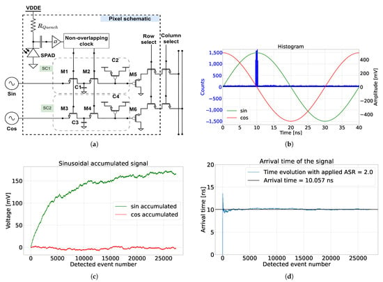
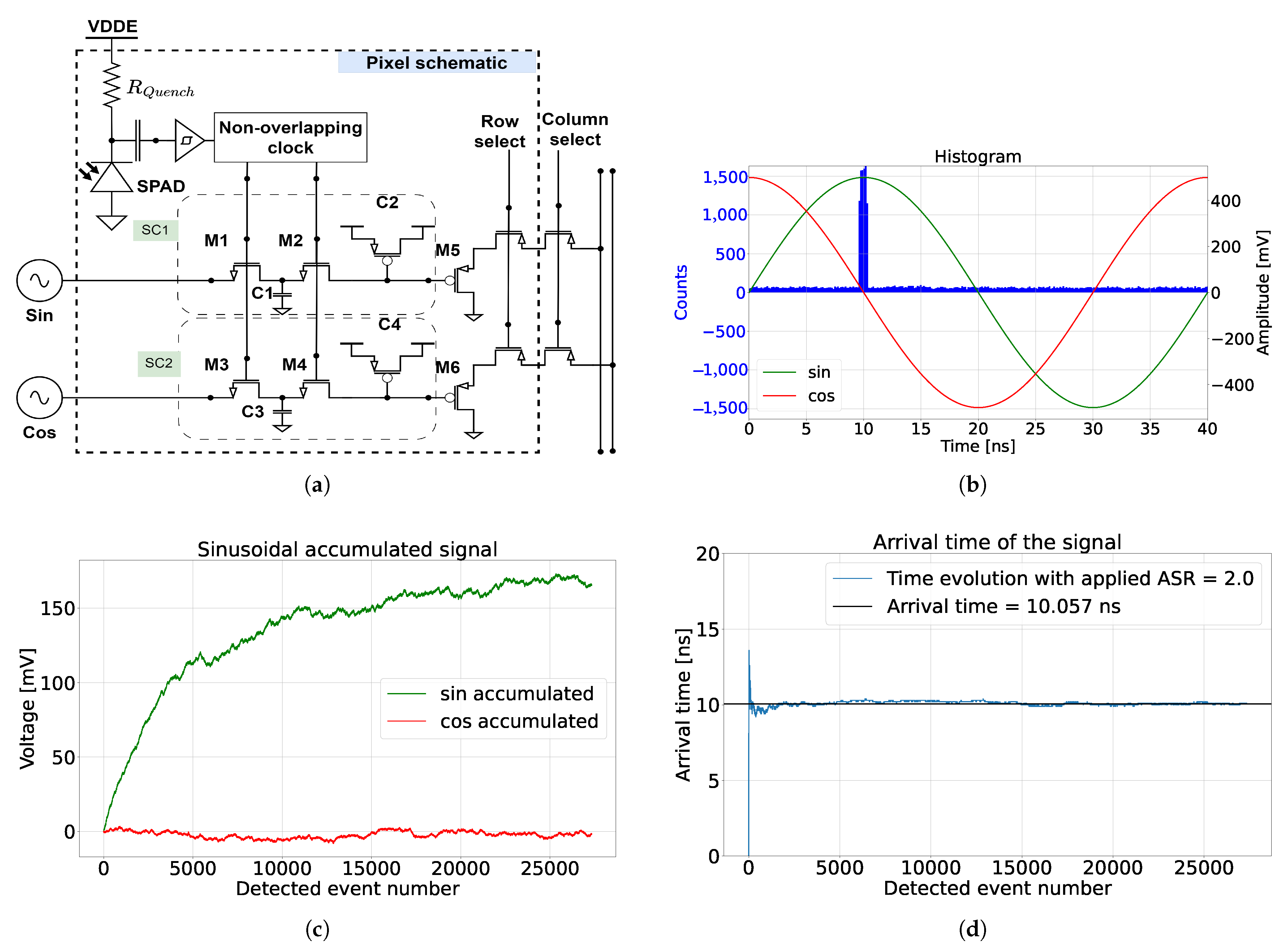
To introduce the operation principle of a correlation-assisted direct time-of-flight (CA-dToF) pixel, we first introduce the pixel schematic in Figure 1a. A laser pulse is synchronized with two orthogonal sinusoidal signals, where the two signals are applied to the pixel as inputs. The pixel utilizes a passively quenched SPAD with a resistor to detect the photon arrival time. The SPAD triggers may originate from the reflected laser pulse, ambient light, or dark count events. When the SPAD is triggered, a non-overlapping clock is generated, driving the two switched capacitor channels ( and for SC1 and and for SC2). Each channel evolves via the following equation:
where is the sampled voltage of the applied sinusoidal signal and is defined as the integration length. Equation (1), known as the exponential weighted moving average (EWMA), is explained in detail in Appendix A. The system is averaging the detected voltage over multiple iterations, with a slow reduction of the weight for a high integration length value , meaning that .
Figure 1.
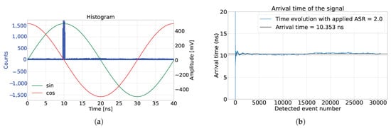
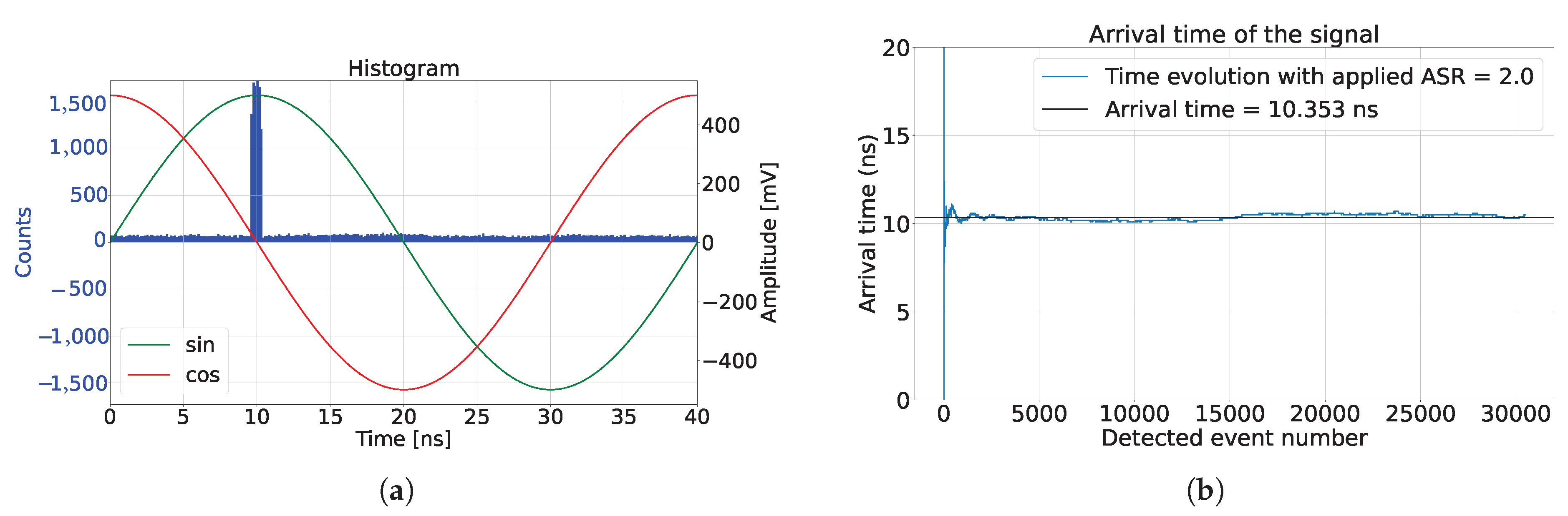
CA-dToF pixel schematic and simulation, where (a) is the pixel schematic and (b) is the histogram from the detected events. On the right side is the sinusoidal signals applied to the CA-dToF pixel, while (c) is the voltage evolution of the analog channels SC1 and SC2 and (d) is the calculated arrival time, with ASR = 2.
The pixel operation involves converting the time-of-arrival information into a voltage. Therefore, it is a form of time-to-amplitude conversion (TAC). To provide intuitive understanding of the system’s operation, a simulation was conducted and presented in Figure 1, where . The simulation presents top-hat laser pulses of 1.7 ns full-width half maximum (FWHM) with an arrival time of 10 ns to a passively quenched SPAD sensor with 5 ns of deadtime. Sinusoidal signals with a 40 ns period were applied for 1000 cycles over the entire simulation period. A histogram of the simulation and the applied signal is depicted in Figure 1b. The ambient light and dark count events were double the applied laser pulse photons, making the ambient-to-signal ratio (ASR) equal two on average. All the incident events before detection followed a Poisson distribution. The simulation result in Figure 1c shows the evolution of the accumulated voltage across the switched capacitor channels SC1 and SC2. The phase evolution of the detected events, which represents the laser pulse arrival time, is calculated and presented in Figure 1d. Notably, the detected phase reached equilibrium after 2000 incident events, while the accumulated voltages required nine times more photons to reach equilibrium. An output reaches equilibrium when the output does not vary significantly anymore, and it oscillates around a certain value. The voltage evolution behavior is known as the inertia effect of the system, which is explained in Appendix A.3. Intuitively, this phenomenon is directly related to the integration length , where the bigger is, the more detected events are needed for the switched capacitor voltage to reach equilibrium. However, as presented in Figure 1d, the inertia effect does not affect the phase information, because the phase is the ratio of the two voltages and not the absolute voltages. As the pixel is exponentially averaging the detected amplitude of the sinusoidal signal, the system does not suffer from saturation or overflow for high input photon flux, as long as the SPAD is not in saturation.
Four key parameters influence pixel operation, which are (1) the number of incident laser and ambient photons, (2) the integration length {}, (3) the laser pulse width {a}, and (4) the applied sinusoidal signal amplitude {C}. To examine pixel behavior, an analytical model of the pixel is provided in Section 3, with emphasis on developing useful tools to extract more information about the environment. The analytical model was validated through simulations under varying conditions, as described in Section 4. The experimental results are detailed in Section 5.
3. CA-dToF Analytical Model
3.1. Ambient Light Influence
The ambient light is not correlated with the arrival time, quantified by a rate {A} (#/ns). Consequently, the arrival time probability distribution is uniformly spread across the integration time. This presumption encompasses light sources such as sunlight and LED sources emitting photons without temporal correlation. However, the assumption excludes light sources exhibiting a specific frequency. For a light source to be categorized as ambient, it must lack correlation with the used active light source, resulting in a uniform distribution in arrival time throughout the integration time. Hence, light sources with harmonics which do not resonate with the active light source remain classified as ambient light, such as indoor lighting and vehicle headlights.
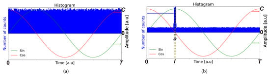
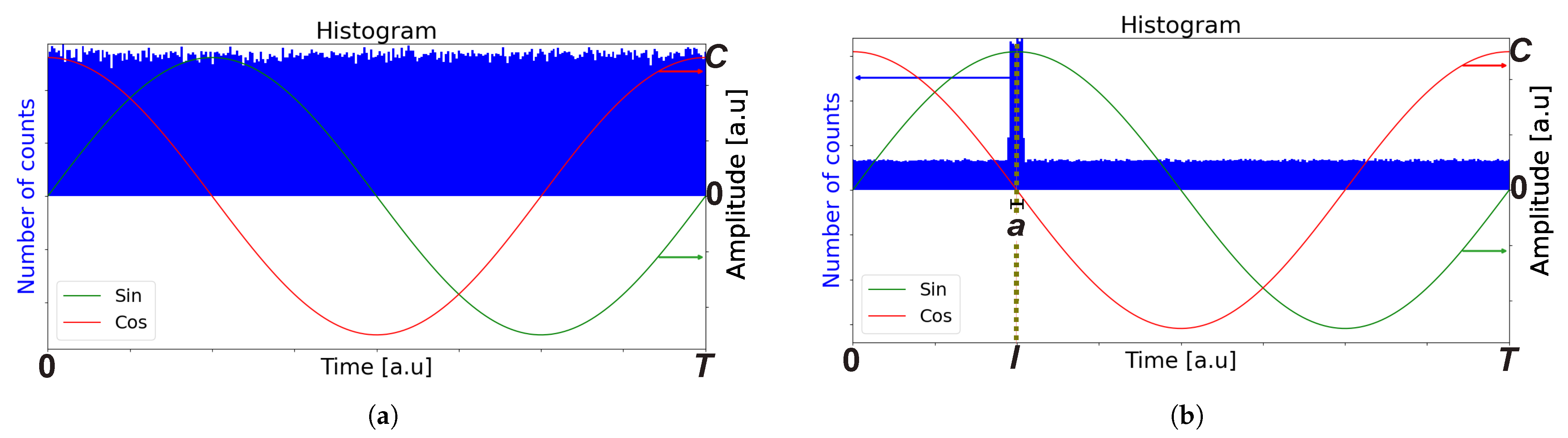
The system utilizes two orthogonal sinusoidal signals with a period T, where each photon detected at time t generates a corresponding voltage such that and , where {C} is the applied signal amplitude shown in Figure 2a. The detected voltages and are independent of each other, indicating that the measurement of one signal does not influence the measurement of the other. Therefore, they can be considered independent variables.
Figure 2.
(a) Histogram of accumulated ambient light over a period {T} for a certain integration time. (b) Histogram of ambient light and laser pulses with an FWHM {a} detected with an arrival time {l} over a period {T}, along with ambient light that is uniformly distributed over the integration time.
The expected values of the variables and over an appropriate integration time can be calculated by integrating the random variables over a period {T} with a uniform probability distribution . The results are
The variance of the random variables and over an appropriate integration time is
where L is the control width, which represents the model tolerance [18]. The physical interpretation of the results can be understood by the fact that the applied sinusoidal signals exhibit intrinsic symmetry around a certain voltage (in this case, ). Consequently, if the probability of detection is equal over the signal period, then the voltage’s expected value converges to zero volts, enabling the system to suppress ambient light. The voltage variance, however, is related to the ambient light shot noise. We will refer to the standard deviation of the detected voltages ( and ) as the amplitude precision.
3.2. Active Light Influence
To simplify the analysis, we considered top-hat laser pulses with a (FWHM) {a} centered around time {l} which were periodically received over a period {T}. When ambient light and laser pulses are applied, the accumulated photons over the integration time are depicted in Figure 2b.
3.3. Expected Value
In the presence of laser pulses, the expected values of the sinusoidal signals and over an appropriate integration time can be calculated in a similar manner to that in the previous section, with the appropriate probability distribution of when there is ambient light and when there is a laser pulse, where {S} is the laser photon arrival rate (#/ns). The expected values are
In Equation (4), we can observe that the norm of and is invariant:
which is referred to as the system’s confidence. For a short laser pulse {a}, and using the small angle approximation, the amplitude is approximated to be where . Consequently, when the system is at equilibrium, ASR is approximately
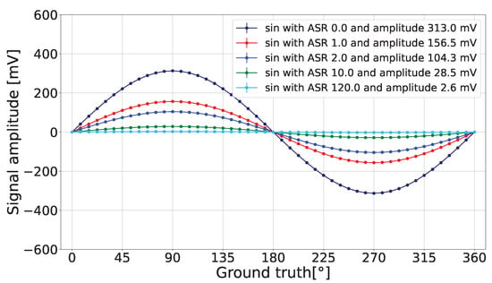
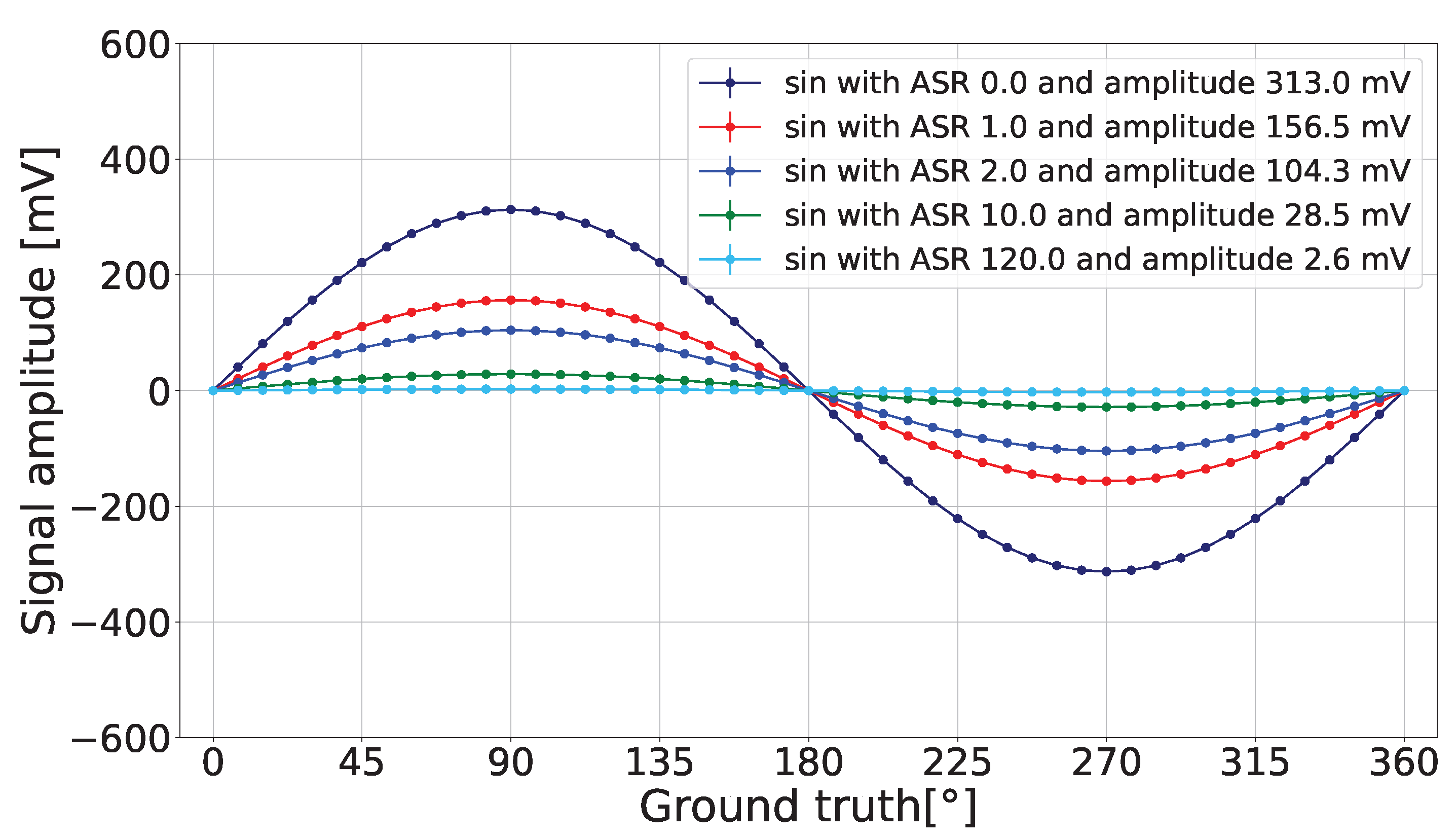
The detected amplitude reduction is visually presented in Figure 3.
Figure 3.
Reduction in the detected sine’s amplitude for different ASR values when and mV.
For the small angle approximation deviation to be , Equation (6) is valid when the pulse width is restricted by the following relation:
For example, if the period is ns, then Equation (6) is valid when ns.
3.4. Variance
The variance in and can be calculated with the same probability distribution shown in Section 3.3 and Equation (A5). The variance equations are
The model demonstrates the relationship between the amplitude precision of the two signals and and the ambient light rate {A}, the signal light rate {S}, the pulse width {a}, and the signal period {T}. It consists of two main terms:
- The ambient shot noise term (), which is directly related to the ambient light;
- The combination of laser and ambient shot noise, which is influenced by the laser pulse width and the ASR.
Notably, through Equations (8) and (9), the amplitude precision can be improved by increasing the integration length {}. Consequently, the system allows counteracting high ambient light effects by adjusting its integration length {} at the cost of increasing the inertia effect.
Section 3.5 is dedicated to providing an intuitive understanding of the amplitude precision behavior.
3.5. Observations
The following figures in this section utilize the parameters mentioned in Table 1, unless mentioned otherwise. Equations (8) and (9) are further explained using the exemplary sine signal. The signal amplitude {C} was chosen to match the detected signal amplitude in the experimental results, explained in Section 5.
Table 1.
Parameter values used in the remainder of this section.
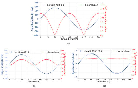
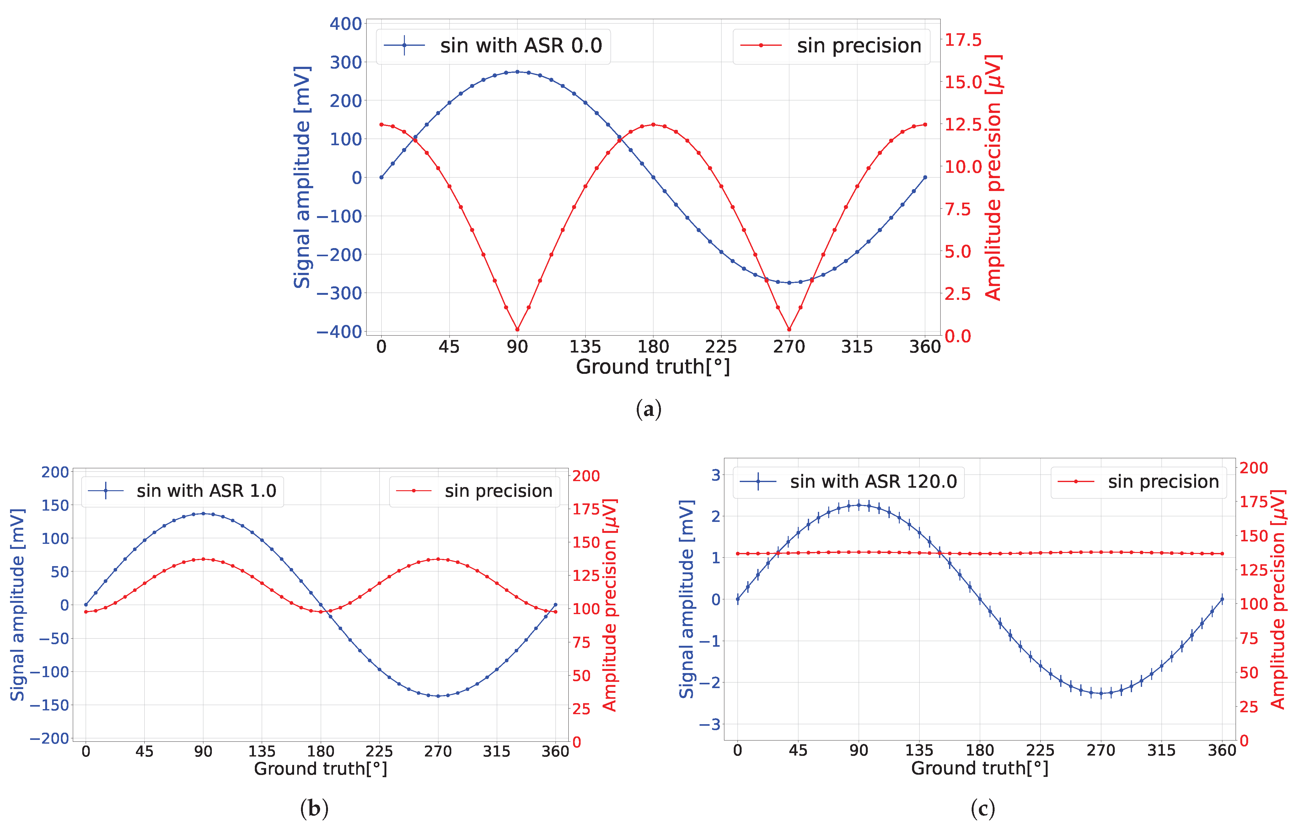
In the absence of ambient light (ASR = 0), the amplitude precision exhibited oscillation, as demonstrated in Figure 4a. To intuitively understand this phenomenon, recall that the pixel converts the time domain of detected events into the voltage domain via sampling and averaging the corresponding sinusoidal signal with a laser pulse width {a}. Consequently, at points where the voltage remains relatively constant over {a} (i.e., at the peaks of the sinusoidal signals), the output voltage remains unaffected by laser shot noise. However, at the inflection point at a angle, fluctuations in the detected voltage occurred due to laser shot noise. The transition from the first case to the latter case resulted in oscillation of the amplitude precision.
Figure 4.
(a) When ASR = 0, the analytical model predicted that the detected voltage precision was oscillating due to active light shot noise. (b) When ASR = 1, the analytical model predicted that the detected voltage precision was oscillating due to the influence of laser and ambient light shot noise. (c) When ASR = 120, the analytical model predicted that the detected voltage precision oscillation was not significant due to the dominant ambient light shot noise.
In the presence of ambient light (ASR = 1), the amplitude precision exhibited a constant shift and an oscillation, as demonstrated in Figure 4b. Due to the ambient light shot noise, a constant amplitude precision offset was imposed on the system. Nonetheless, laser shot noise continued to impact the amplitude precision, with heightened oscillations occurring particularly when the laser aligned with sinusoidal peaks.
To explain this behavior, recall that the resultant output voltage stems from averaging across the entire signal and fluctuations due to both laser and ambient shot noise. Therefore, the voltage fluctuation was influenced by the amplitude difference between the measured voltage amplitude and the remaining sinusoidal signal amplitude. Consider the sine peak point at a angle and the inflection point at a angle. Given that the maximum amplitude difference within the sinusoidal signal was between its peaks, the detected fluctuation attained its maximum when the laser pulse captured the peak voltage of the angle. Conversely, when examining the angle, the discrepancy between the measured voltage amplitude and any peak amplitude was minimized, resulting in the least amount of voltage fluctuation.
3.6. Phase Calculation
After estimating the expected amplitude and amplitude precision of the sinusoidal signals, the phase information can be extracted via the equation . However, due to the nonlinear relation between the functions, the phase’s expected value and variance are approximated using Taylor expansion. The average phase after the EWMA is
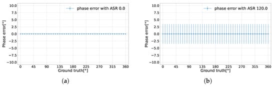
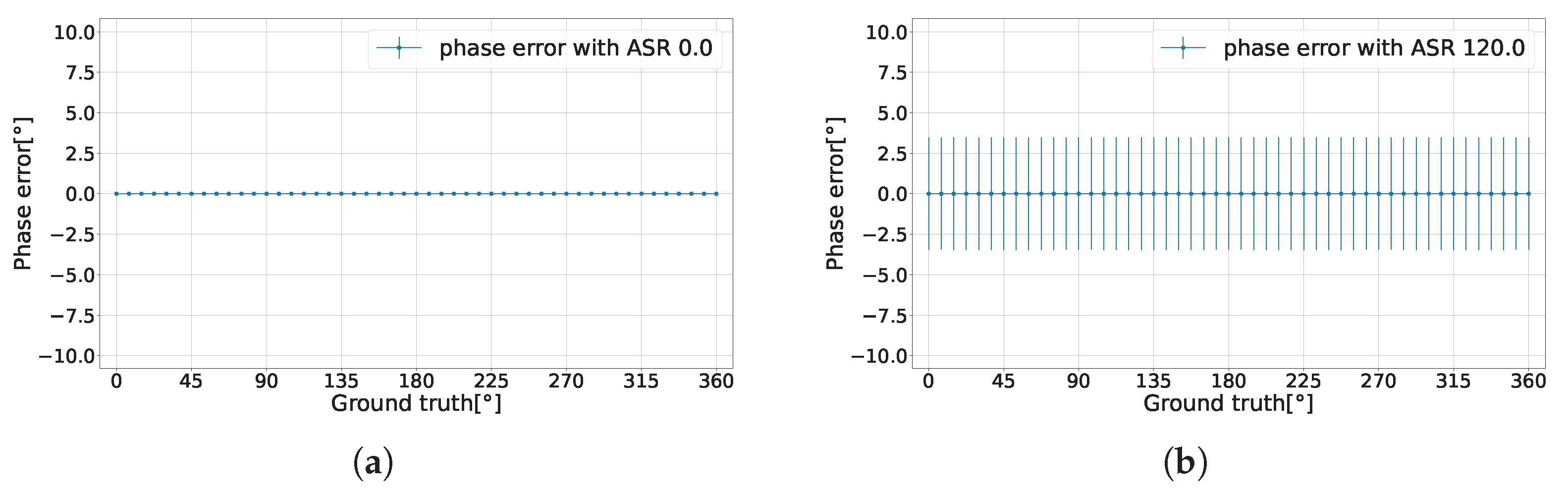
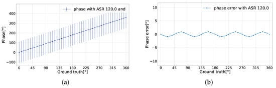
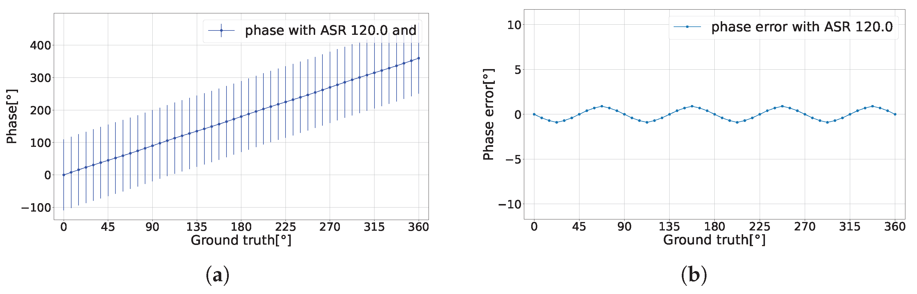
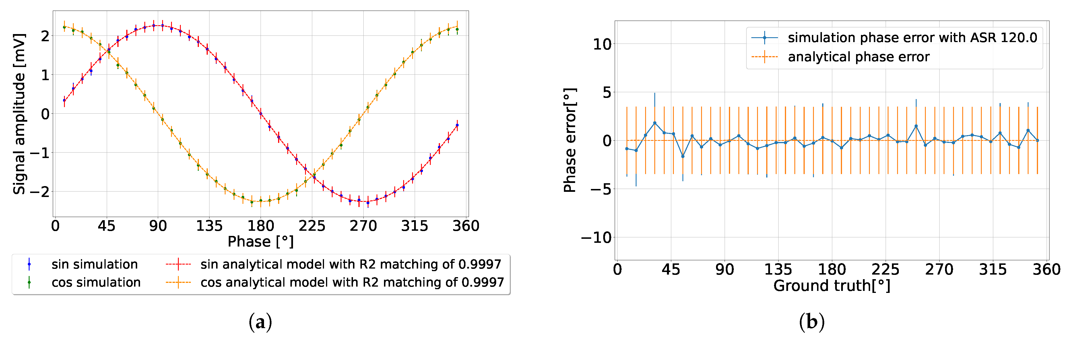
The findings reveal a notable characteristic of the CA-dToF system. For the phase’s expected value , the variance in the two analog channels due to ambient shot noise was effectively eliminated, leaving only the variance related to the laser pulse width as shown in Figure 5a,b with a phase precision less than 1% of the detection range when ASR = 120. The difference between the ground truth and the phase expected value is defined as the phase error. The laser pulse width contributes to the oscillation in the phase error in the case of extreme ASR and low integration length , as shown in Figure 6.
Figure 5.
Analytical phase error with the corresponding phase precision. (a) When ASR = 0. (b) When ASR = 120.
Figure 6.
(a) Phase’s expected value with the ground truth when ASR = 120 and . (b) Phase error without the corresponding phase precision.
The phase precision was derived from the combination of the analog channel variances. Unlike the phase’s expected value, the phase precision increased, corresponding to the variance in both analog channels. Nevertheless, it was possible to reduce the phase precision by increasing the integration length .
The analytical model does not account for the effect of the SPAD deadtime. To examine the impact of deadtime and validate the analytical model, a separate statistical model was developed.
4. Statistical Model
The pixel is statistically simulated by considering two assumptions: (1) the SPAD generates a digital pulse when triggered, and (2) when the SPAD is triggered, the system evolves via EWMA as presented in Equation (1). The simulation did not explicitly consider the characteristics of the detected object nor the sensor’s dark count rate, as they could be implicitly included in the ASR. The ASR was fixed through the detection range, eliminating the effect of signal reduction for various distances. Ambient light was randomly generated over time, and the laser pulse was a top-hat laser pulse with a fixed pulse width {a}. The number of photons over one period followed a Poisson distribution for all events. Two orthogonal sinusoidal signals were sampled simultaneously when the SPAD was triggered, making both signals have the same phase when detected. The parameters used in the simulation are summarized in Table 2. The simulation input parameters were chosen to match the measurement input parameters, as explained in Section 5.
Table 2.
The parameters used for the statistical model.
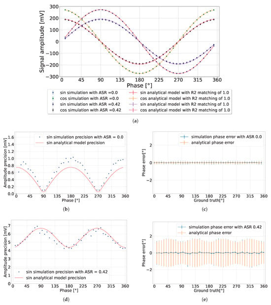
There were multiple simulations conducted to verify the analytical model developed in Section 3 in the absence of the deadtime effect. The focus was on varying the ambient light level and the integration length. The latter allowed avoiding the inertia effect within a limited number of cycles.
4.1. Various Ambient Light Conditions
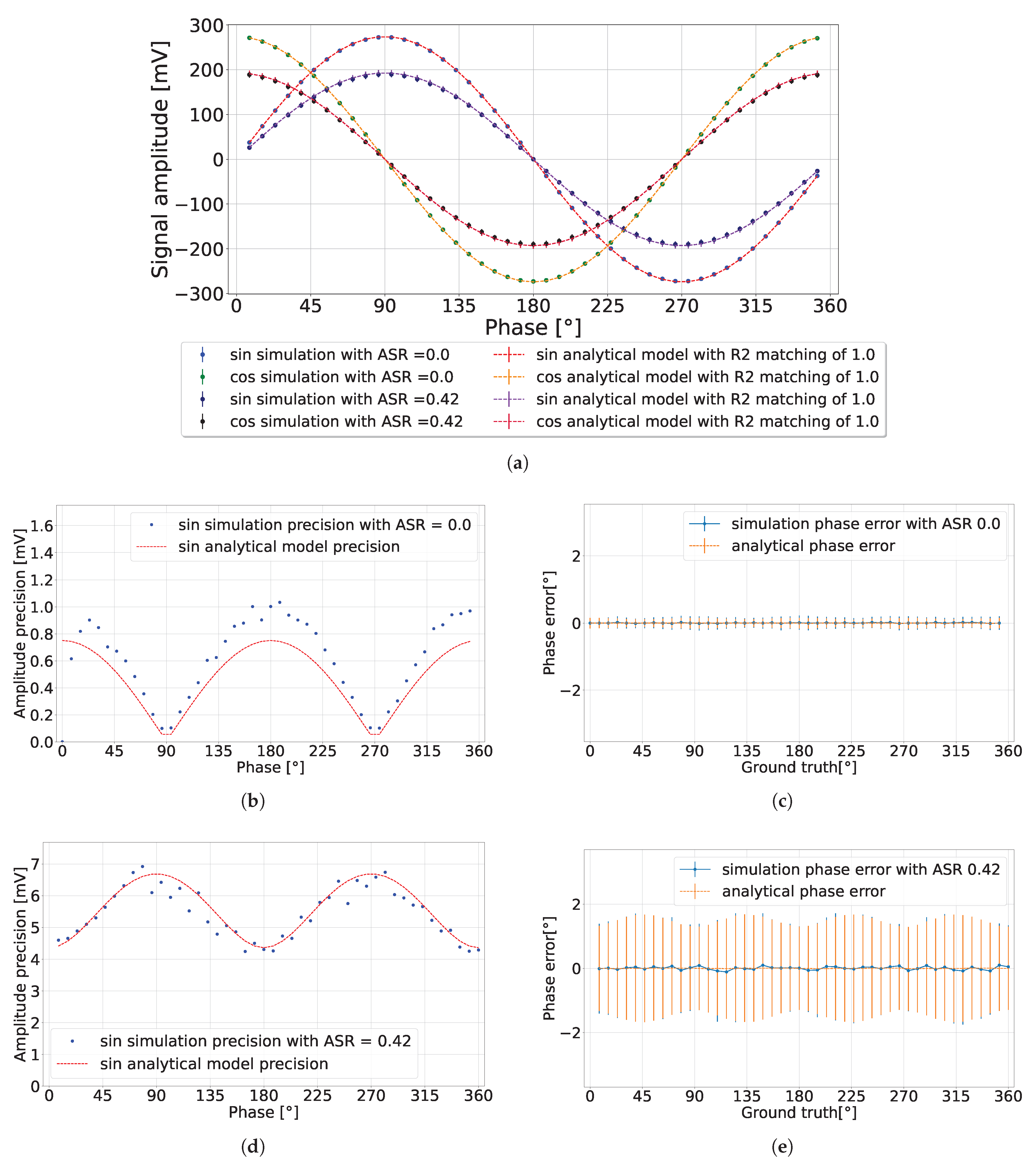
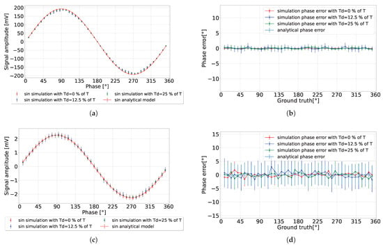
This subsection presents the pixel simulations, comparing them with the developed analytical model presented in Section 3 with the lowest precision tolerance (L = 1). In the simulation results presented in Figure 7, with , each data point was derived from an average of 300 measurements to calculate the detected signal’s expected value and amplitude precision. It can be observed in Figure 7b that in the absence of ambient light (ASR = 0), the amplitude precision exceeded the predicted value by 0.25 mV. This discrepancy may be attributed to our choice of using the lowest precision tolerance of the analytical model (L = 1). Hence, it allowed for the possibility of greater observed amplitude precision. Conversely, when ASR = 0.42, the amplitude precision aligned closely with the predicted analytical model as presented in Figure 7d. The calculated phase error is presented in Figure 7c,e, showing consistent results with the analytical model.
Figure 7.
CA-dToF simulation results when for two different ASR values. (a) Detected signal amplitude. (b,c) Amplitude precision and phase error when ASR = 0, respectively. (d,e) Amplitude precision and phase error when ASR = 0.42, respectively.
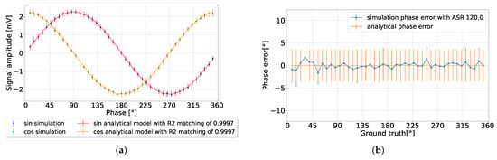
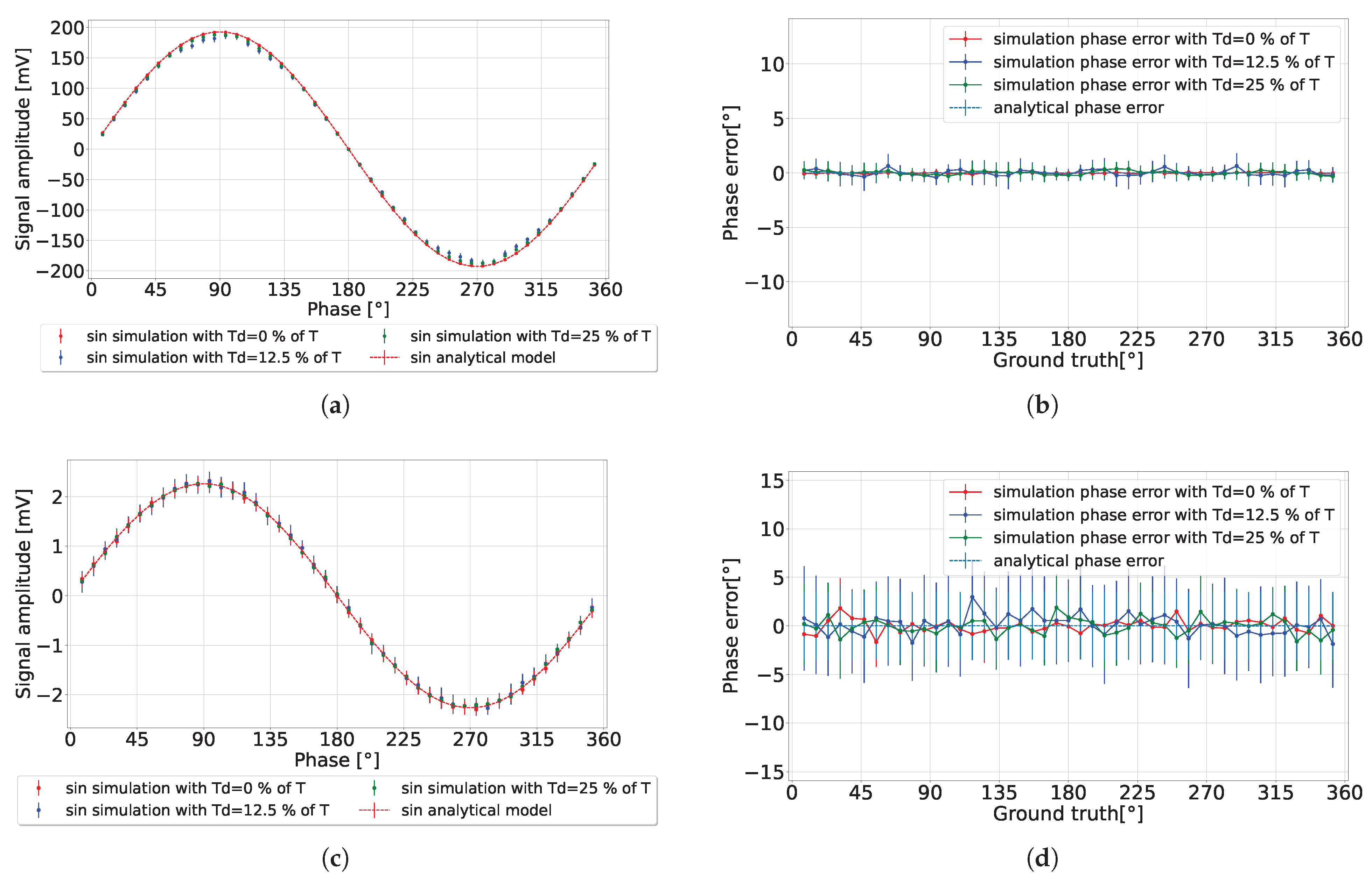
By changing the environment to a high ambient light setting (ASR = 120 for ), as presented in Figure 8, the detected signal exhibited a significant reduction in amplitude, matching the analytical model results. Concurrently, the amplitude precision was reduced by increasing the integration length, thereby achieving a phase precision that fell below 1% of the detection range, without discrepancy in the phase error. One observation of high ambient light conditions is the diminished detected amplitude, which imposes a constraint on the operational range of the analog-to-digital converter (ADC).
Figure 8.
CA-dToF simulation results for when ASR = 120. (a) Detected signal. (b) Phase error.
This subsection compared the analytical and statistical results, presenting consistent results between both models. However, the pixel operation was affected by the SPAD deadtime. We explore the deadtime effect on the pixel operation in the following section.
4.2. Deadtime Shadowing Effect
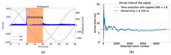
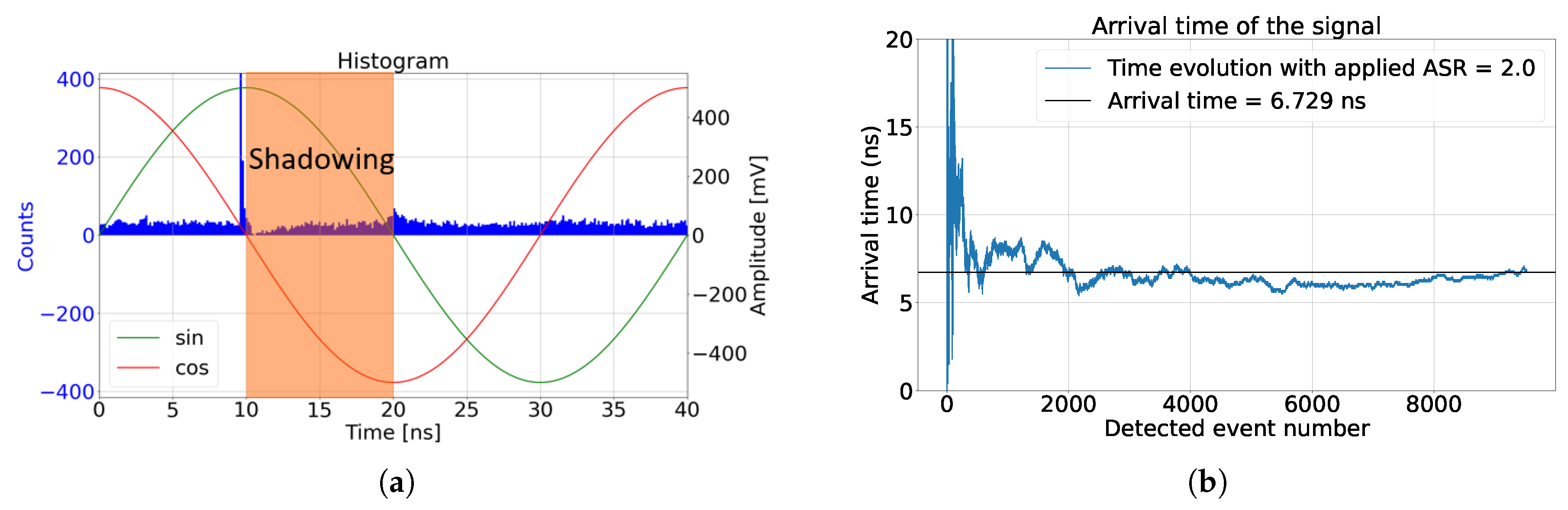
The SPAD deadtime is the time taken for the SPAD to fully recharge into the Geiger operation mode. In our simulation, the SPAD was passively quenched with a resistor. The excess biased voltage of the SPAD charges exponentially, as explained in [19]. If we assumed that the SPAD’s photon detection probability (PDP) was zero during the deadtime, then the detected ambient light was not uniform, as presented in Figure 9. This phenomenon is known as the pile-up effect [17]. However, the operation of the CA-dToF is different than that in the histogram method. Therefore, we refer to this deadtime effect as the deadtime shadowing effect, where the SPAD deadtime shadows the rest of the active signal and the detected ambient light, making the ambient light nonuniform over the applied signal and creating a phase offset which depends on the ambient light level. In the remainder of this section, an investigation is conducted to predict the deadtime shadowing effect over CA-dToF’s operation.
Figure 9.
CA-dToF simulation results when ASR = 2 with applied laser pulses arriving at 10 ns and an SPAD deadtime of 10 ns, including a PDP of 0 during the deadtime. (a) Detected signal with SPAD deadtime shadowing effect and (b) detected phase.
The assumption that the PDP is zero can be challenged when using a passively quenched SPAD. As mentioned in [20], the SPAD PDP can be approximated to have a linear response with the excess bias. Hence, by considering the increase in the SPAD PDP with the exponential increase in the excess bias, we noticed that the shadowing effect was significantly reduced, as illustrated in Figure 10. One conclusion drawn from this analysis is that the deadtime shadowing effect can be nulled by a sufficient number of photons in the detected laser pulses.
Figure 10.
CA-dToF simulation results, including a PDP relative to the SPAD excess bias during the deadtime. (a) Detected signal and (b) detected phase.
To investigate further, we implemented a passively quenched SPAD with different deadtime values to our simulator, neglecting the voltage threshold of the detection circuit after the SPAD. The results are presented in Figure 11. We scanned the full range of detection when ASR = 0.42 and , as presented in Figure 11a,b. The same scenario was also simulated when ASR = 120 and , as depicted in Figure 11c,d. The simulation showed that the shadowing effect did not impact the phase error with different deadtime values or different environmental conditions.
Figure 11.
CA-dToF simulation results for two different SPAD deadtime values for when ASR = 0.42. (a) Detected sine signal and (b) phase error. When ASR = 120 and , (c) is the detected sine signal, and (d) is the phase error.
Mitigation of the shadowing effect can be achieved through the employment of multiple SPADs per pixel. In this configuration, each SPAD is coupled with a switched capacitor circuit, and the resultant signal output is integrated within a larger switched capacitor. This approach serves to further alleviate the shadowing effect by enabling the independent triggering of multiple SPADs.
Additionally, an alternative method for mitigating the shadowing effect involves the utilization of SPAD active quenching synchronized with the signal period {T}. This strategy effectively eliminates the shadowing effect by ensuring that the detection occurs only once within each signal period. This solution relies on the fact that when one photon is detected per period, the ambient light detection becomes uniform, thus facilitating ambient light averaging and subsequent mitigation of the shadowing effect. Conversely, the system would require a higher number of cycles to reach equilibrium, consuming more power on average and having a lower frame rate. The shadowing effect was not observed when our experimental work was conducted, as presented in Section 5.
5. Experimental Results
5.1. Experimental Set-Up
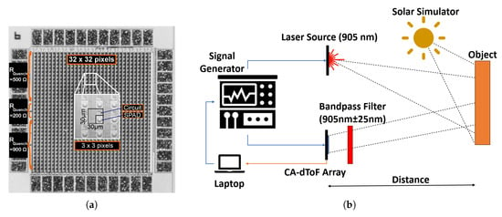
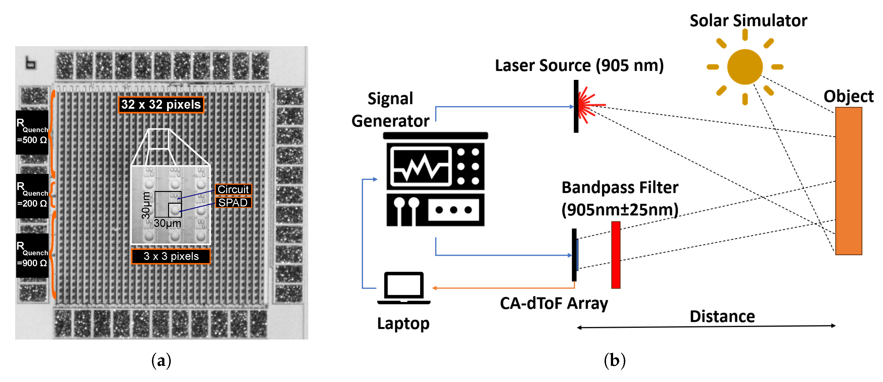
Following the statistical analysis of the system operation, experimental work was conducted. A pixel array schematic, presented in Figure 1a, was fabricated using X-FAB 180 nm technology with a pixel pitch of 30 m, as presented in Figure 12a. The sinusoidal signals were synchronized with a 905 nm high-power pulsed laser source with a top-hat pulse width of 1.8 ns using a signal generator. Sinusoidal signals with a 25 MHz repetition rate were applied to the full array with per analog channel. The pixel array featured an identical circuit structure across the array, except for the quenching resistor . Three different values for the quenching resistors were used—200 k, 500 k, and 900 k—as presented in Figure 12a. The quenching resistor variations were meant to test the deadtime variation effect over the pixel operation. The exact deadtime was not accessible to be detected. However, the deadtime was expected to be higher for a higher-resistance quenching resistor.
Figure 12.
(a) CA-dToF pixel array micrograph with three different quenching resistors. (b) The experimental set-up.
The experimental set-up is presented in Figure 12b, with a solar simulator device (Hal-302) utilized as the ambient light source to emulate sunlight.
5.2. Measurement Method
To align the analytical and statistical models with the experimental work, the ASR had to remain constant across the detection range. Therefore, the distance between the CA-dToF array and the object was fixed, thereby preventing ASR degradation over varying distances. Object movement was mimicked by shifting the applied sinusoidal signal using the signal generator, which scanned the entire detection range. Additionally, we measured the circuit behavior across the full detection range at different ASR levels. The applied sinusoidal signals had a peak-to-peak voltage of 1.20 V. As shown in Figure 1a, the voltages of the switched capacitor stages (SC1 and SC2) were detected through two PMOS source followers ( and ).
To account for the source follower offset of the sinusoidal signal , a differential measurement was employed. In this method, two detected measurements were shifted , which was achieved by shifting either the applied laser or the applied signal . For example, for the sine signal, the detected voltages were and , where represents the detected amplitude of the sinusoidal signal. By averaging the two measurements, the offset voltage was determined. Another method for detecting the voltage offset is by measuring ambient light only without any laser signal. In this case, the average voltage should theoretically reach zero, indicating the offset of the source follower, as discussed in Section 3.1. However, this method relies on the assumption that the system’s switched capacitor and the source follower responses are linear across the entire detection range. Observations indicated that this linearity was not maintained over the full range of detection, leading to the decision to not use this method in our measurements.
The experiment was conducted using the set-up illustrated in Figure 12b. Both the ambient light and laser source were projected onto an object with an approximate reflectivity coefficient of 24% for the wavelength used. The object remained at a constant distance throughout the detection period. To prevent SPAD saturation, the ambient light was filtered using a bandpass filter centered near a 905 nm wavelength. Each distance was measured 1024 times to determine the signal amplitude mean and amplitude precision associated with each point. This data analysis aimed to identify the system’s minimum amplitude precision to align the results with the analytical model. Consequently, the control width L in Equations (8) and (9) was set to one. The used SPAD had a PDP of 5% for a 905 nm wavelength.
5.3. Experimental Results
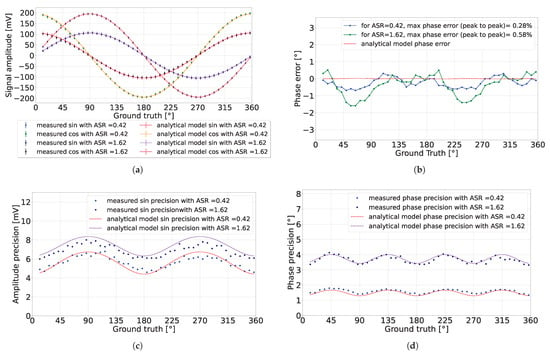
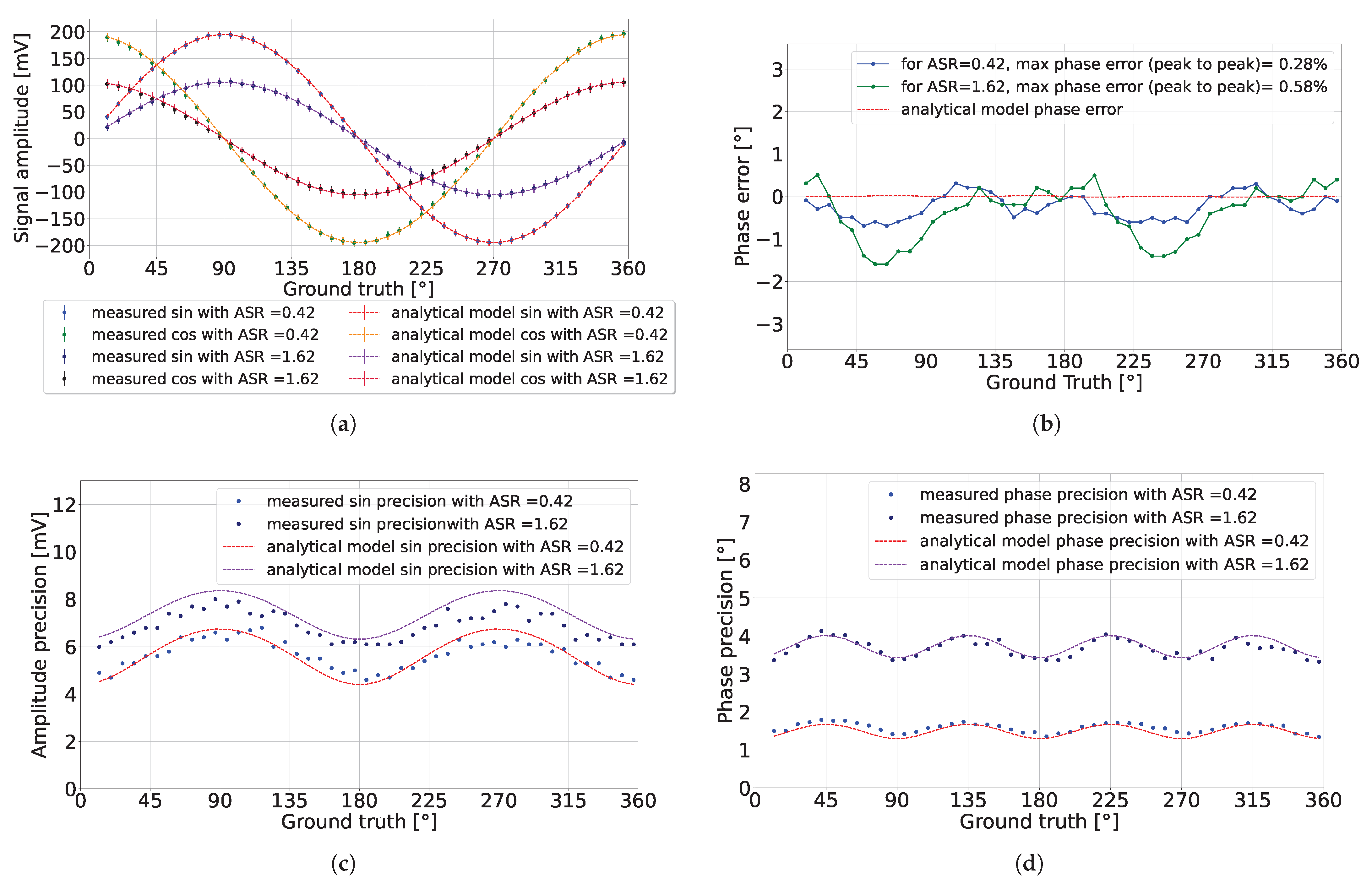
The detected signal over the full phase range is presented in Figure 13, with ASR values of 0.42 and 1.61. Figure 13a shows the detected sinusoidal amplitude relative to the ground truth in the phase, with a phase step delay of applied by the signal generator. The ground truth is expressed in terms of its phase rather than time to generalize the measurement for testing the pixel operation independent of the applied signal period. The analytical model with the same parameters is also plotted in the figure. The pixel used for this result had an SPAD quenching resistor of 500 k.
Figure 13.
CA-dToF pixel experimental results for two different ASR values: (a) detected signal, (b) detected phase error, (c) detected amplitude precision, and (d) detected phase precision.
The detected sinusoidal signals exhibited different amplitudes at 20 mV, possibly due to a gain mismatch between the source followers of the two analog channels. After calibration, the maximum deviation between the analytical model and the measurements was near 8 mV. This difference in sinusoidal amplitudes translated into cyclic phase error, as shown in Figure 13b.
The precision in the detected sine amplitude, shown in Figure 13c, matched the behavior predicted by the analytical model, with a similar pattern observed for the detected cosine amplitude precision. The amplitude precision in the detected sinusoidal signals translated into the phase precision, illustrated in Figure 13d, which also aligned with the predictions of the analytical model.
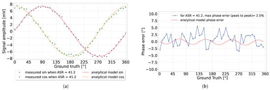
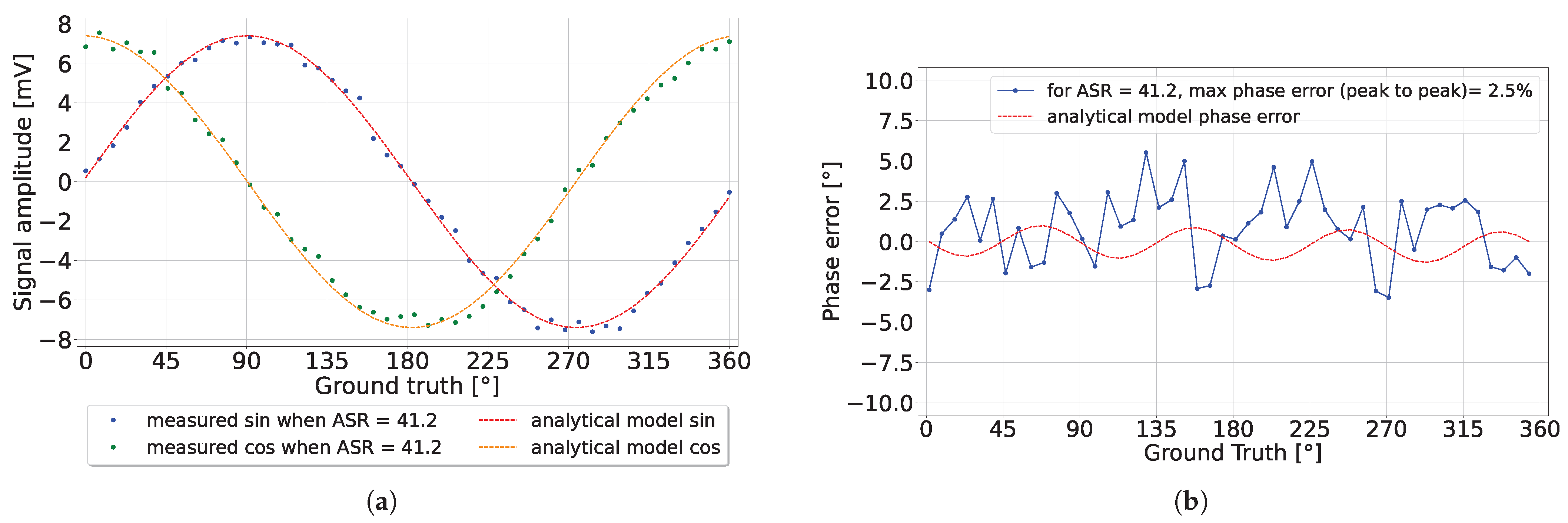
Under a high ASR of 41.2, the detected signal amplitude approximately matched the analytical model. However, the overwhelming ambient light shot noise affected the detected phase, causing the phase error to oscillate, as shown in Figure 14b. The phase precision was omitted from this figure due to its high value of approximately . Overall, the results between the analytical model and the measurements consistently matched.
Figure 14.
The detected sinusoidal amplitude (a) and phase error (b) when ASR = 41.2.
The pixels consumed 40 W per pixel on average, including the SPAD operation, two switched capacitor circuits, and an in-pixel counter. The power consumption of the supporting systems, such as the laser source and the generated signals, was not considered, as we were focused on characterizing the pixel operation.
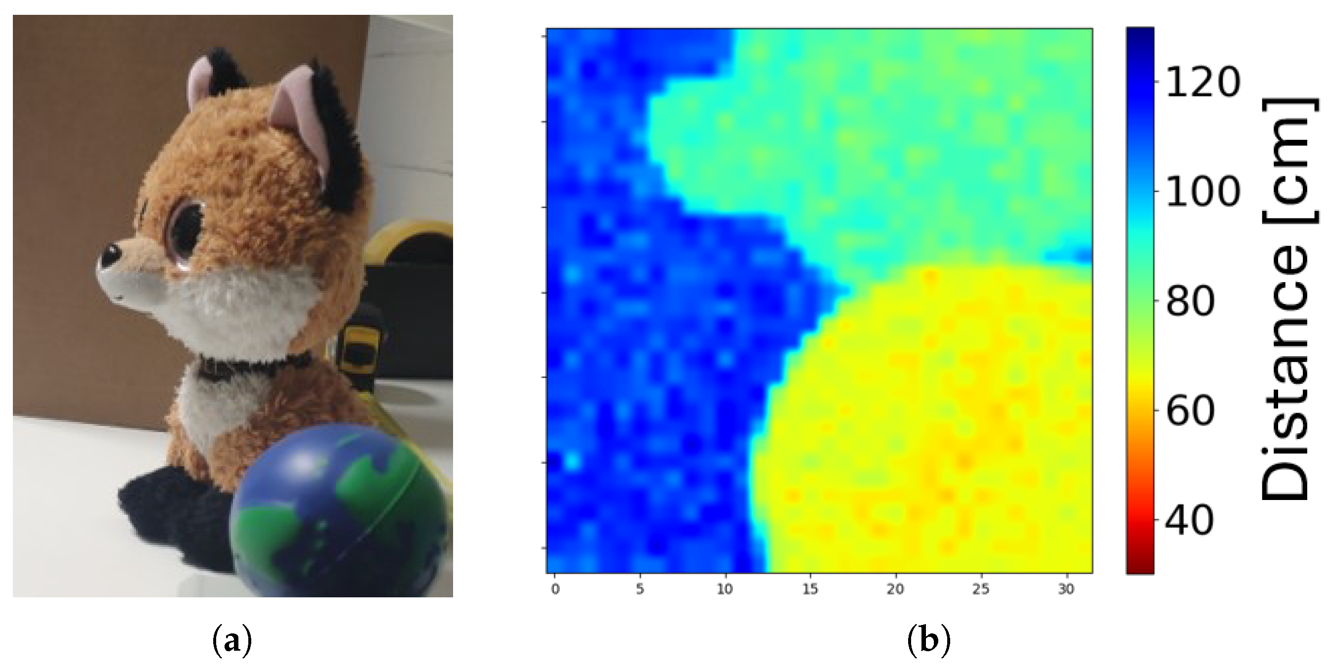
To characterize the SPAD deadtime shadowing effect, two pixels with 200 k and 900 were tested at a fixed detected distance. If there was a deadtime shadowing effect, then we expected phase degradation with different ambient light conditions for different deadtime values, leading to a distance error. Table 3 presents two pixels with different quenching resistors, detecting the same distance with two different ASR conditions. The maximum distance error detected was 0.3% for a 6 m detection range. The phase error did not present reliable evidence of the shadowing effect. In Figure 15, a 3D image and a colored image were captured by the pixel array over a 1 m range.
Table 3.
A fixed distance point was analyzed over data samples to detect the shadowing effect over the detected distance. The ground truth is the distance when ASR = 0, and the error is the difference between the ground truth and the detected distance when the ASR is high for the same pixel, divided by the full detection range of 6 m.
Figure 15.
A snapshot of a scene with the pixel array at the room’s ambient light. (a) Colored image of the scene. (b) The 3D image.
Table 4 presents a comparison between our pixel operation and different dToF pixels. The key criterion was the pixel power consumption, which indicates the scalability of a pixel array. Pixel precision was not considered, as the presented pixel was limited by its internal integration length. The primary source of power consumption in the CA-dToF pixel is the SPAD sensor, with the pixel circuit consuming four times less power compared with the SPAD.
Table 4.
Comparison of performance with different dToF pixels.
6. Conclusions and Discussion
This paper introduced the operation of a correlation-assisted direct time-of-flight (CA-dToF) imaging sensor which utilizes an SPAD-based pixel array and sinusoidal signals correlated with a pulsed laser source. The pixel operation was comprehensively analyzed using an analytical model and validated through statistical modeling and experimental work. The pixel operation conceptually depends on the laser pulse width, the ASR, the sinusoidal signal period and amplitude, and the integration length of the pixel.
The operational range of the pixel depended on the applied sinusoidal signal period. However, the detected precision decreased over longer ranges. Another challenge was phase wrapping in the detected signal, which led to distance detection ambiguity. To maintain high-precision detection and avoid phase wrapping, gating the sinusoidal signal is a viable solution. This method involves initially applying a frame with a long period {T} to estimate the approximate distance of the object. Subsequently, a second frame with a gated sinusoidal signal of a period {T}/n, where n is an integer, is applied to the pixel, being gated around the object’s approximate distance. The first frame provides a rough estimate of the object’s distance, while the second frame offers higher precision and a more accurate distance measurement.
The pixel operation did not directly account for environmental effects. The reflectivity of the detected object and its location affected the ASR of the detected signal. The frame rate of the pixel depended on the integration length, the detected environment, and the SPAD sensitivity to the detected wavelength. The analytical model in Section 3 was based on the assumption that the pixel-detected voltages reached equilibrium. However, for a high integration length value , a high frame rate, and a low ambient light level, the inertia effect, discussed in Section 2, may lead to inaccurately detected voltages, causing a mismatch between the analytical model and the measurement. Under a low light condition and a high frame rate, the inertia effect can cause errors in the detected confidence and phase. To overcome this challenge, one possible solution is to dedicate testing pixels with a low integration length, which reach equilibrium faster, and to use their data for checking if the pixels reach equilibrium. Another suggestion is to develop variable capacitors in-pixel to adjust the pixel integration length, depending on the environmental conditions. However, this solution requires an extra system to detect the outside environment’s photon flux.
Additionally, the SPAD deadtime is not considered in the analytical model. We address in Section 4.2 the SPAD deadtime shadowing effect on the phase and propose possible mitigation methods. Other environmental conditions which affect ToF technologies such as the scattering environment, multi-path reflections, and transparent objects are also challenges to the proposed CA-dToF pixel. More studies are required to understand the influence of such challenges on CA-dToF pixel operation.
Author Contributions
Conceptualization, M.K.; Methodology, A.M.; Software, A.M.; Validation, A.M.; Formal analysis, A.M.; Investigation, A.M.; Resources, M.K.; Writing—original draft, A.M.; Writing—review & editing, M.K.; Visualization, A.M.; Supervision, M.K.; Project administration, M.K.; Funding acquisition, M.K. All authors have read and agreed to the published version of the manuscript.
Funding
This research was in part funded by Vrije Universiteit Brussel (VUB) through SRP 78 grants.
Data Availability Statement
Data are contained within the article.
Acknowledgments
We would like to thank Jonathan Ernest J. Vrijsen, Jan Coosemans, Tuur Bruneel, and Sevada Sahakian for their insightful discussions and valuable feedback for this article.
Conflicts of Interest
The authors declare no conflicts of interest.
Abbreviations
The following abbreviations are used in this manuscript:
| EWMA | Exponential weighted moving average |
| CA-dToF | Correlation-assisted direct time-of-flight |
| ASR | Ambient-to-signal ratio |
| PDP | Photon detection probability |
Appendix A. Exponential Weighted Moving Average
Exponential moving average, geometrical moving average, and exponential weighted moving average (EWMA) are various names for the same averaging method. It is an average where the previous measurements are exponentially decrementing their weight over new iterations. To observe this behavior, the general equation is
as , which is the weight. To understand the behavior of , let us observe the evolution of the equation:
With Equation (A2), we can define the weighted factor as
Appendix A.1. Properties
The first observation regarding is its convergence to one over infinite iterations, as calculated below:
where the term is a geometric series. The observation implies that if there is a constant voltage measured over infinite iterations, then the output voltage converges to . For and , the weighted factor is dwindling as shown in Figure A1a,b, respectively.
Figure A1.
Measurement weight evolution when (a) and (b) . The blue bar indicates the effect of the new measurement on the previous measurement weight.
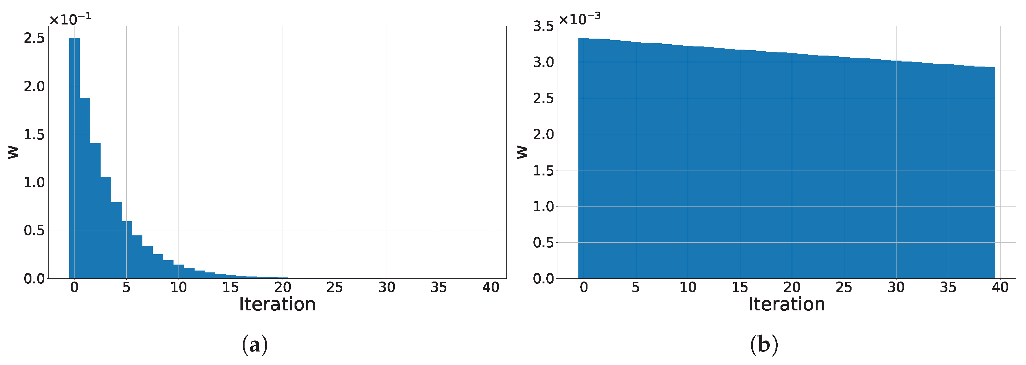
An important observation here is that for a smaller , the decay of is slower over new iterations. Hence, for small values, the EWMA can be used to approximate the usual arithmetic mean for a certain detection period. But when mentioning the detection period, we assume that the rate of detection is fast enough that the system reaches equilibrium. If the detection rate is insufficient, then the system cannot converge to the average value. The inertia effect is further discussed in Appendix A.3.
Appendix A.2. EWMA Standard Deviation
If a system generates random and uncorrelated measurements with a variance , then the variance of the EWMA is reduced as shown in the following the equation [18]:
For an infinite number of iterations, the variance converges to a steady state:
where and L is the control width, which represents the tolerance of the model at which the system is still under control and is tuned by the system data.
This result implies that (1) the variance of the system is filtered out via the EWMA process, and (2) the smaller the value, the lower the variance output of the system. These conclusions are interesting, as there is control over the variance of the system by controlling the value.
Appendix A.3. Inertia Effect
To have a better understanding of the weight factor , we sum the weight of a measurement after N iterations. Using Equation (A3), we can find that
Equation (A6) provides an important relationship between the number of iterations N and the weight evolution . For example, to have 99% of the measurement weight, the neglected weight is . The number of iterations to reach a certain lower weight is calculated to be
For example, let with an initial weight measurement . For this measurement weight to reach of the initial weight, the neglected weight is . The number of iterations is , with a weight . This result implies that with a smaller value, the initial weight decay is slower, enabling better averaging. However, the system’s response to a sudden change is poor for a small value. It requires multiple iterations to react to the change in the measurement, meaning that the EWMA system has “inertia” against new changes in the system. This inertia effect reduces the effectiveness of adapting to a new change in the system.
References
- Horaud, R.; Hansard, M.; Evangelidis, G.; Ménier, C. An overview of depth cameras and range scanners based on time-of-flight technologies. Mach. Vis. Appl. 2016, 27, 1005–1020. [Google Scholar] [CrossRef] [Scilit]
- Bamji, C.; Godbaz, J.; Oh, M.; Mehta, S.; Payne, A.; Ortiz, S.; Nagaraja, S.; Perry, T.; Thompson, B. A Review of Indirect Time-of-Flight Technologies. IEEE Trans. Electron Devices 2022, 69, 2779–2793. [Google Scholar] [CrossRef] [Scilit]
- Bamji, C.S.; Mehta, S.; Thompson, B.; Elkhatib, T.; Wurster, S.; Akkaya, O.; Payne, A.; Godbaz, J.; Fenton, M.; Rajasekaran, V.; et al. IMpixel 65 nm BSI 320 MHz demodulated TOF Image sensor with 3 μm global shutter pixels and analog binning. In Proceedings of the 2018 IEEE International Solid-State Circuits Conference—(ISSCC), San Francisco, CA, USA, 11–15 February 2018; pp. 94–96. [Google Scholar] [CrossRef] [Scilit]
- Keel, M.S.; Jin, E. A VGA Indirect Time-of-Flight CMOS Image Sensor With 4-Tap 7-μm Global-Shutter Pixel and Fixed-Pattern Phase Noise Self-Compensation. IEEE J. Solid-State Circuits 2020, 55, 889–897. [Google Scholar] [CrossRef] [Scilit]
- Kim, D.; Lee, S.; Park, D.; Piao, C.; Park, J.; Ahn, Y.; Cho, K.; Shin, J.; Song, S.M.; Kim, S.J.; et al. Indirect Time-of-Flight CMOS Image Sensor With On-Chip Background Light Cancelling and Pseudo-Four-Tap/Two-Tap Hybrid Imaging for Motion Artifact Suppression. IEEE J. Solid-State Circuits 2020, 55, 2849–2865. [Google Scholar] [CrossRef] [Scilit]
- Ebiko, Y.; Yamagishi, H.; Tatani, K.; Iwamoto, H.; Moriyama, Y.; Hagiwara, Y.; Maeda, S.; Murase, T.; Suwa, T.; Arai, H.; et al. Low power consumption and high resolution 1280 × 960 Gate Assisted Photonic Demodulator pixel for indirect Time of flight. In Proceedings of the 2020 IEEE International Electron Devices Meeting (IEDM), San Francisco, CA, USA, 12–18 December 2020; pp. 33.1.1–33.1.4. [Google Scholar] [CrossRef] [Scilit]
- Kawahito, S.; Yasutomi, K.; Mars, K. Hybrid Time-of-Flight Image Sensors for Middle-Range Outdoor Applications. IEEE Open J. Solid-State Circuits Soc. 2022, 2, 38–49. [Google Scholar] [CrossRef] [Scilit]
- Mars, K.; Sakai, K.; Nakatani, Y.; Hakamata, M.; Yasutomi, K.; Lioe, D.X.; Kagawa, K.; Akahori, T.; Kosugi, T.; Aoyama, S.; et al. A 648 × 484-Pixel 4-Tap Hybrid Time-of-Flight Image Sensor with 8 and 12 Phase Demodulation for Long-Range Indoor and Outdoor Operations. In Proceedings of the 2023 International Image Sensor Workshop, Scotland, UK, 21–25 May 2023. [Google Scholar] [CrossRef]
- Miyazawa, R.; Shirakawa, Y.; Mars, K.; Yasutomi, K.; Kagawa, K.; Aoyama, S.; Kawahito, S. A Time-of-Flight Image Sensor Using 8-Tap P-N Junction Demodulator Pixels. Sensors 2023, 23, 3987. [Google Scholar] [CrossRef] [Scilit] [PubMed]
- Hatakeyama, K.; Okubo, Y.; Nakagome, T.; Makino, M.; Takashima, H.; Akutsu, T.; Sawamoto, T.; Nagase, M.; Noguchi, T.; Kawahito, S.; et al. A Hybrid ToF Image Sensor for Long-Range 3D Depth Measurement Under High Ambient Light Conditions. IEEE J. Solid-State Circuits 2023, 58, 983–992. [Google Scholar] [CrossRef] [Scilit]
- Hauser, M.; Zimmermann, H.; Hofbauer, M. Indirect Time-of-Flight with GHz Correlation Frequency and Integrated SPAD Reaching Sub-100 µm Precision in 0.35 µm CMOS. Sensors 2023, 23, 2733. [Google Scholar] [CrossRef] [Scilit] [PubMed]
- Hutchings, S.W.; Johnston, N.; Gyongy, I.; Al Abbas, T.; Dutton, N.A.W.; Tyler, M.; Chan, S.; Leach, J.; Henderson, R.K. A Reconfigurable 3-D-Stacked SPAD Imager With In-Pixel Histogramming for Flash LIDAR or High-Speed Time-of-Flight Imaging. IEEE J. Solid-State Circuits 2019, 54, 2947–2956. [Google Scholar] [CrossRef] [Scilit]
- Villa, F.; Lussana, R.; Bronzi, D.; Tisa, S.; Tosi, A.; Zappa, F.; Dalla Mora, A.; Contini, D.; Durini, D.; Weyers, S.; et al. CMOS Imager With 1024 SPADs and TDCs for Single-Photon Timing and 3-D Time-of-Flight. IEEE J. Sel. Top. Quantum Electron. 2014, 20, 364–373. [Google Scholar] [CrossRef] [Scilit]
- Markovic, B.; Tisa, S.; Villa, F.A.; Tosi, A.; Zappa, F. A High-Linearity, 17 ps Precision Time-to-Digital Converter Based on a Single-Stage Vernier Delay Loop Fine Interpolation. IEEE Trans. Circuits Syst. Regul. Pap. 2013, 60, 557–569. [Google Scholar] [CrossRef] [Scilit]
- Tancock, S.; Arabul, E.; Dahnoun, N. A Review of New Time-to-Digital Conversion Techniques. IEEE Trans. Instrum. Meas. 2019, 68, 3406–3417. [Google Scholar] [CrossRef] [Scilit]
- Gyongy, I.; Erdogan, A.T.; Dutton, N.A.; Martín, G.M.; Gorman, A.; Mai, H.; Rocca, F.M.D.; Henderson, R.K. A Direct Time-of-Flight Image Sensor With In-Pixel Surface Detection and Dynamic Vision. IEEE J. Sel. Top. Quantum Electron. 2024, 30, 3800111. [Google Scholar] [CrossRef] [Scilit]
- Gyongy, I.; Dutton, N.A.W.; Henderson, R.K. Direct Time-of-Flight Single-Photon Imaging. IEEE Trans. Electron Devices 2022, 69, 2794–2805. [Google Scholar] [CrossRef] [Scilit]
- Roberts, S.W. Control Chart Tests Based on Geometric Moving Averages. Technometrics 1959, 1, 239–250. [Google Scholar] [CrossRef]
- Xue, X.; Ji, C.; Yuan, Y.; Sun, K.; Rosenmann, D.; Guha, S. Dynamic-quenching of a single-photon avalanche photodetector using an adaptive resistive switch. Nat. Commun. 2022, 13, 1517. [Google Scholar] [CrossRef] [Scilit]
- Mahmoudi, H.; Poushi, S.S.K.; Steindl, B.; Hofbauer, M.; Zimmermann, H. Optical and Electrical Characterization and Modeling of Photon Detection Probability in CMOS Single-Photon Avalanche Diodes. IEEE Sens. J. 2021, 21, 7572–7580. [Google Scholar] [CrossRef] [Scilit]
- Zhang, C.; Lindner, S.; Antolović, I.M.; Mata Pavia, J.; Wolf, M.; Charbon, E. A 30-frames/s, 252 × 144 SPAD Flash LiDAR With 1728 Dual-Clock 48.8-ps TDCs, and Pixel-Wise Integrated Histogramming. IEEE J. Solid-State Circuits 2019, 54, 1137–1151. [Google Scholar] [CrossRef] [Scilit]
- Zhang, C.; Zhang, N.; Ma, Z.; Wang, L.; Qin, Y.; Jia, J.; Zang, K. A 240 × 160 3D-Stacked SPAD dToF Image Sensor With Rolling Shutter and In-Pixel Histogram for Mobile Devices. IEEE Open J. Solid-State Circuits Soc. 2022, 2, 3–11. [Google Scholar] [CrossRef] [Scilit]
- Stoppa, D.; Abovyan, S.; Furrer, D.; Gancarz, R.; Jessenig, T.; Kappel, R.; Lueger, M.; Mautner, C.; Mills, I.; Perenzoni, D.; et al. A reconfigurable QVGA/Q3VGA Direct time-of-flight 3D imaging system with on-chip depth-map computation in 45/40 nm 3D-stacked BSI SPAD CMOS. In Proceedings of the International Image Sensor Workshop (IISW), Virtual, 20–23 September 2021; pp. 53–56. [Google Scholar]

Disclaimer/Publisher’s Note: The statements, opinions and data contained in all publications are solely those of the individual author(s) and contributor(s) and not of MDPI and/or the editor(s). MDPI and/or the editor(s) disclaim responsibility for any injury to people or property resulting from any ideas, methods, instructions or products referred to in the content. |
© 2024 by the authors. Licensee MDPI, Basel, Switzerland. This article is an open access article distributed under the terms and conditions of the Creative Commons Attribution (CC BY) license (https://creativecommons.org/licenses/by/4.0/).