Preliminary Observations of Environmental Effects on Immature Whale Shark Surface Feeding Behaviour in Nosy Be, Madagascar

Abstract

Nosy Be in the northwestern Madagascar hosts one of the largest known seasonal feeding aggregations of whale sharks. However, the environmental drivers influencing whale shark surface feeding behaviour in this area remain poorly understood. This study investigates the relationship between environmental variability and surface feeding strategies of immature whale sharks at Nosy Be. Boat-based surveys were conducted in November 2018, 2019, 2022, and 2023, resulting in the photo-identification of 88 individuals and the recording of 85 surface feeding events. The influence of environmental factors on feeding behaviour was assessed using multicollinearity among the environmental covariates and three-level step approach: permanova, multinomial logistic regression, marginal effects, and Cochran’s Q, to evaluate whether environmental conditions discriminate feeding-behaviour categories and to quantify how individual covariates relate to behavioural composition under a multi-step framework. Results showed that there is not a strong enough predictive signal for behaviour based on environmental variables; however, thanks to the marginal effects, it is possible to better assess the probability of a certain type of eating behaviour in the presence of an increase in one of the environmental variables, for example, chlorophyll-a appears to be the most interesting, because its increase is associated with a greater probability of some behaviours instead the others. These preliminary observations provide the first insights to evaluate environmental influences on immature whale shark surface feeding behaviour in Nosy Be, highlighting that it is therefore necessary to deepen and increase data collection to have long and significant series of data, integrated also with data on the preys subject to feeding behaviour and to evaluate which other unobserved aspects, perhaps linked precisely to the consistency and quality of the prey, could allow us to predict feeding behaviour. Improving the understanding of these relationships is essential for predicting whale shark habitat use and for supporting conservation and management strategies in a region increasingly affected by climate variability and anthropogenic pressures.

1. Introduction

In the Mozambique Channel, Nosy Be island is a high productivity site and the topography of the shelf area off north-western Madagascar favours the presence of fast-growing zooplankton and micronekton [1]. This high productivity and the great density of available prey promote the presence of plankton-feeding megafauna, including whale sharks (Rhincodon typus, Smith, 1828) [1]. The productivity period, corresponding to the austral summer, allows whale shark aggregations around Nosy Be which are strongly linked to physical oceanographic processes occurring off the northern Mozambique coast [1]. Previous studies showed that the cool, chlorophyll-a–rich surface waters in this region are generated by coastal upwelling driven by alongshore north-easterly monsoon winds prevailing from August to March. These nutrient-enriched waters are subsequently transported offshore by anticyclonic and cyclonic eddies that reach the coast of Nosy Be [2,3].

Nosy Be is known to host one of the largest known whale shark seasonal feeding aggregations [4,5]. This species seasonally aggregates in Nosy Be from September to December, using this area as a foraging ground and the aggregation is mainly composed of immature individuals [1]. This aggregation allowed the frequent observation of whale sharks at surface exhibiting feeding behaviours. Several studies demonstrated that whale sharks preferentially feed on zooplanktonic prey [6,7,8,9,10,11,12], but also on fish spawn [13,14] and fast-swimming prey, such as fish [1,5,15,16]. In Nosy Be, preliminary studies on zooplankton surface abundance and composition reported that zooplankton was mainly represented by holoplanktonic organisms such as Copepoda, followed by Appendicularia, Mollusca and Chaetognata taxa [8,17]. Although there is a lack of data on the whale shark feeding ecology, Whitehead and Gayford [18] showed that whale sharks also actively feed on benthic prey either predominantly in deepwater environments or where the abundance of such prey exceeds that of planktonic food sources. Anyway, the possibility to predict whale sharks’ aggregations will allow us to gather more insights on this topic.

Several authors [19,20,21] have described different whale shark surface feeding behaviours. The most common ones are those reported by Nelson and Eckert [22], who highlighted three main filter-feeding techniques exhibited in relation to specific zooplankton sources, resulting in an energy gain greater than the actual energy cost following the theory of optimal foraging. Ram (or simply passive) feeding occurs when zooplankton density is low. The whale shark swims slowly in a straight line with a horizontal posture, keeping its mouth slightly to fully open without gulping. The gills are lifted or open, and prey enters the mouth as the shark moves forward just below the surface. Active surface ram (or simply active) feeding occurs at high zooplankton density. The shark opens and closes its mouth rhythmically, performing gulping movements, sometimes with the upper jaw emerging above the surface. The gills pump rhythmically while swimming is more vigorous, with frequent turns and surface-oriented movements. This mode combines both ram- and suction-feeding. Vertical (suction or simply vertical) feeding occurs at moderate zooplankton density. The shark adopts a vertical or slightly diagonal posture near the surface with little or no forward motion, hovering or slowly rotating. The mouth and gills move rhythmically as the shark uses suction feeding to ingest large volumes of water at a fixed location.

Environmental factors that could influence the whale shark surface feeding behaviour and shifts in prey are still poorly known [23,24]. Whale shark behavioural patterns seem to be associated not only with food availability at coastal locations but also with climatic and oceanographic processes such as ENSO (El Niño Southern Oscillation), upwelling, coastal current and fronts, cloud coverage, sea conditions, sea surface temperature, wind speed, precipitation, time of the day, sea surface chlorophyll-a concentration and bathymetry [7,24,25,26,27,28]. All these factors may potentially control the distribution and abundance of prey at surface. Indeed, there is also growing concern that climate change may impact whale shark feeding behaviour due to indirect effects such as changes to their habitat, food availability and densities, representing a significant challenge to their survival and conservation efforts [29].

While several studies investigated the effects of some environmental factors on whale shark surface sightings and moving patterns [9,27,30,31,32,33], only three studies described the environmental drivers of whale shark surface feeding behaviour. However, while Motta et al. [34] and Gleiss et al. [35] showed in Cabo Catoche (Mexico) and Ningaloo Reef (Australia), respectively, the correlation between the time of the day and the whale shark feeding technique adopted, Reinero et al. [24] described for the first time the overall effects of environmental factors on the whale shark surface feeding behaviour in Djibouti. The authors reported that sea surface chlorophyll-a (SSC) concentration, in turn influenced by other environmental variables, was the main parameter predicting the selection of filter-feeding techniques [24]. Specifically, active and vertical feeding behaviours were associated with rainfall, lower sea surface temperature (SST), worse sea conditions, and low wind speed during the morning, conditions that enhance SSC concentrations. In contrast, passive feeding was favoured during opposite environmental conditions [24]. Additionally, El Niño events promoted passive and vertical feeding behaviours, whereas active feeding was more prevalent during La Niña events [24].

In Madagascar, studies examining the influence of environmental factors on whale shark surface feeding behaviour are currently lacking. However, predictors linked to oceanographic processes such as ENSO and associated wind patterns and SSTs, together with local (SSC and cloud coverage) environmental factors, may influence not only whale shark distribution and abundance but also feeding behaviour and prey availability, thereby affecting the selection of filter-feeding techniques in relation to prey density.

Given this important knowledge gap, understanding the environmental drivers of whale shark surface feeding behaviours is essential for informing conservation management of this endangered species in Madagascar, where coastal aggregations in Nosy Be may be exposed to multiple threats associated with ecotourism activities. Accordingly, this study aims to: (1) analyze if observed feeding behaviours are not driven by uneven sampling effort across the different sampling windows, (2) if observed feeding behaviour patterns could be distorted by variation in observation effort, (3) the surface feeding behaviours exhibited by whale sharks in relation to environmental factors and (4) verify if environmental factors are associated with different surface feeding strategies in order to predict potential future scenarios.

2. Materials and Methods

2.1. Study Area

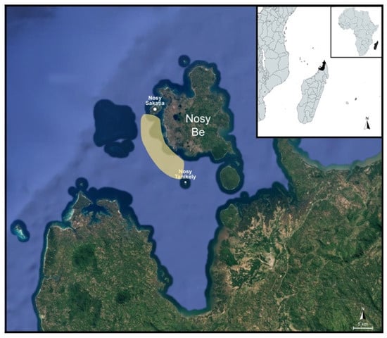
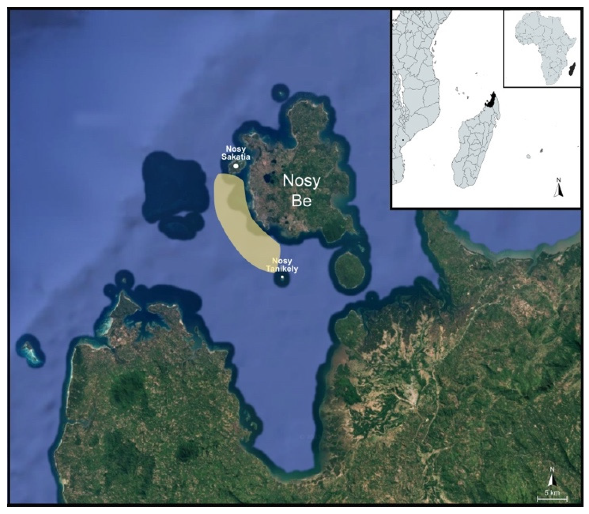
Nosy Be (13°39′ S, 48°20′ E; Figure 1), meaning “big island” in the Malagasy language, is located approximately 8 km off the northwestern coast of Madagascar in the Mozambique Channel. It forms an archipelago with several smaller surrounding islands, including Nosy Fanihy, Nosy Sakatia, Nosy Faly, Nosy Ambariobe, Nosy Tanikely, Nosy Komba, Nosy Mamoko, and Nosy Tonga. Nosy Be is of volcanic origin, covers an area of approximately 312 km², and reaches a maximum elevation of 450 m at Mont Lokobe. Sea surface temperatures range from about 24 °C in August to 28–30 °C in February [17]. Four scientific expeditions were conducted in 2018, 2019, 2022, and 2023, excluding the SARS-CoV-2 pandemic years of 2020–2021. Sampling activities were carried out in November of each year, which corresponds to the peak season for whale shark surface sightings [5].

Figure 1. Nosy Be (Madagascar) and the sampling area between Nosy Sakatia and Nosy Tanikely.

2.2. Whale Shark Sightings and Identification

Boat-based surveys for whale sharks were conducted along the southwestern coast of Nosy Be Island, with logistical support from the partner operator Manta Diving. Surveys were carried out during the morning hours (approximately 09:00–13:00), when sea conditions were generally more favourable. Overall, approximately 160 h of monitoring were conducted over the four study years, specifically, in 2018, two weeks, 2019, one month, 2022, one week, and in 2023, one week. The spatial coverage of surveys between Nosy Sakatia and Nosy Tanikely was not fixed but included an area comprising within 5 km from the coast; search routes and distances varied depending on whale shark sightings. A team of at least eight trained volunteers and research staff from the Sharks Studies Centre–Scientific Institute of Massa Marittima, Italy, collected standardized data. All interactions with sharks adhered to the Madagascar Government and whale shark codes of conduct [36]. To minimize disturbance, groups of four people at a time entered the water gently from the boat, always maintaining a minimum distance of three metres from the animals.

Whale sharks were frequently observed feeding at the surface in association with zooplankton patches and bait balls formed by mackerel tuna feeding on juvenile fish, which typically attracted seabirds. These areas are known locally as “chasse” due to intense surface activity and are generally visible from a certain distance [5]. Once a whale shark was sighted, snorkelers approached it underwater to photograph and film both flanks above the pectoral fins, just posterior to the gill slits, using action cameras (in housing GoPro Hero 7, 8, 9, 10, 11, 12 underwater cameras USA) for photo-identification. Individual identification was based on the unique spot patterns present in this region of each shark [37]. Body scars and wounds were also documented to support individual identification [22]. Operators swam beneath the whale shark to determine its sex by checking for the presence of claspers within the pelvic fins [22]. Whale shark partial sizes were measured using laser-photogrammetry from the mouth to the base of the first dorsal fin [24,33], and total length (TL) was subsequently calculated using the equation proposed by Matsumoto et al. [38]. However, laser-photogrammetry was only employed in 2022 and 2023; in previous years (2018 and 2019), size measures were taken by comparison with the dimensions of the boat and measures were not considered for greater accuracy of estimates.

Photographs were then uploaded to the I³S (Interactive Individual Identification System) Classic pattern recognition software v4.0 to evaluate matches among specimens [24,33]. For each sighted and recorded shark, the following information was documented: identification number, photos of both flanks, date and location of sighting, sex (if determined), TL (if available), associated videos and photo references, and the position of scars and wounds. If the same shark was resighted multiple times during the same or different years, only the first recorded sighting was considered.

Videos were analyzed to classify the surface feeding behaviours exhibited by the sharks, and only footage in which both the mouth and gills were clearly visible was used. Feeding activities were categorized as passive (P), active (A), or vertical (V) following the criteria described by Nelson and Eckert [22]. The frequency of each behaviour was calculated as a percentage (%). It should be noted that individual sharks could be observed multiple times throughout the day, and all exhibited behaviours were recorded.

2.3. Environmental Data Collection

Environmental variables were collected during all scientific expeditions (2018, 2019, 2022, and 2023), either measured in situ or obtained from international databases as follows:

(1)

Sea sSurface temperatures (SST), expressed in degrees Celsius (°C) was obtained by Climate Re-analyser database https://climatereanalyzer.org/research_tools/monthly_tseries/ (accessed on 15 January 2024).

(2)

Wind speed, expressed in knots, was obtained by Visual Crossing programme https://www.visualcrossing.com/excel-weather/ (accessed on 15 January 2024).

(3)

Sea Surface Chlorophyll-a (SSC) concentration, expressed in mg/m3, was obtained by Copernicus Marine Data Storage programme https://marine.copernicus.eu/it/accesso-dati (accessed on 15 January 2024).

(4)

Cloud coverage, expressed in oktas, represents the fraction of the sky obscured by clouds in eighths [39]. The following intervals were used to categorize sky conditions: 0–2 oktas for clear sky, 3–5 oktas for partly cloudy sky, and 6–8 oktas for overcast sky. Cloud coverage data were obtained from the Visual Crossing programme https://www.visualcrossing.com/excel-weather/ (accessed on 15 January 2024).

(5)

El Niño Southern Oscillation (ENSO), expressed in Multivariate ENSO Index (MEI), was obtained by NOAA Physical Sciences Laboratory database https://psl.noaa.gov/enso/mei/ (accessed on 15 January 2024).

2.4. Statistical Analysis

This study assessed 85 recorded surface feeding behaviours (from individuals exhibiting at least one feeding behaviour) across four time periods (2018, 2019, 2022, and 2023). The dataset contains both quantitative and qualitative variables. The formers correspond to five environmental factors: SST (°C), SSC (mg/m³), ENSO (MEI), cloud coverage (oktas), wind speed (knots); the latter correspond to the three different feeding behaviours: active (A), passive (P), and vertical (V) feeding. SST, SSC, ENSO, and wind speed were categorized as scale-level variables. The cloud coverage is categorized as an ordinal level variable characterized by ranks as follows: 1 = 0–2 oktas; 2 = 3–5 oktas; 3 = 6–8 oktas. The feeding behaviour is a nominal variable.

2.4.1. Are Observed Feeding Behaviours Not Driven by Uneven Sampling Effort Across the Different Sampling Windows?

To verify that the observed feeding behaviours are not driven by uneven sampling effort across the different sampling windows, two complementary checks were implemented using the observation date and the ordinal coding of feeding behaviour (V < P < A), corresponding to vertical, passive, and active feeding behaviour. Weeks were defined as International Organization for Standardization (ISO) weeks of the year. Because several week-by-category cells are sparsely populated, model-based inference was used alongside a parsimonious contingency-table comparison. (A) Week-of-year effect net of inter-annual heterogeneity. A proportional-odds ordinal logit with year fixed effects (FE) was estimated, and the week-of-year block was evaluated through a likelihood-ratio (LR) test comparing models with vs. without the week factor. (B) Early vs. late sampling window. As a robustness simplification, observations were grouped into an earlier (ISO week ≤ 48) and a later (ISO week > 48) sampling window, and independence between this two-level timing indicator and feeding behaviour was tested using Pearson’s chi-squared test. Effect size was summarized by Cramér’s V.

2.4.2. Observed Feeding Behaviour Patterns Could Be Distorted by Variation in Observation Effort? Or Does the Number of Feeding Behaviours Depend on the Number of Whale Sharks Observed?

To evaluate whether the observed feeding behaviour patterns could be distorted by variation in observation effort, a composition-based check was performed using the daily sampling record. Observations with missing date or feeding behaviour were excluded. Feeding behaviour was treated as a three-level categorical outcome (V, P, A). For each sampling day, the total number of observation records was computed and interpreted as a proxy for the number of whale-shark “sightings” recorded that day (daily_sightings). In parallel, the number of ‘A’ events recorded on the same day (A_count) was calculated. The response of interest was the daily proportion of ‘A’ behaviours, operationalised through a binomial likelihood with A_count successes out of daily_sightings trials. A baseline intercept-only model was compared to an extended model including daily_sightings as a predictor. The incremental contribution of daily sightings was assessed via an LR test (deviance difference).

To assess whether any apparent association was robust and not driven by between-year heterogeneity or isolated high-leverage sampling days, four complementary sensitivity analyses were carried out. First, the binomial models were refitted including year fixed effects and the LR test was repeated for the addition of daily_sightings. Second, a quasi-binomial specification was estimated to allow for potential extra-binomial variation, and inference on the daily_sightings slope was based on the corresponding Wald test (with the estimated dispersion parameter φ). Third, influential-point diagnostics were computed using Cook’s distance under the unadjusted daily model; the most influential day was removed and the LR test was recomputed (leave-one-out sensitivity). Fourth, the data were aggregated at the ISO week level within year (year–week periods), and the year-adjusted LR test was repeated using weekly totals (sightings) and weekly A counts.

2.4.3. Multicollinearity Checks Among Environmental Covariates

Multicollinearity among the environmental covariates (sst, chl_a, enso, cloud_cov, wind_speed) was assessed using pairwise correlation analysis and variance inflation factors (VIF). Prior to computing these diagnostics, the data were restricted to complete cases across the five covariates, and all variables were coerced to numeric format; observations producing missing values after coercion were excluded. Pearson correlation coefficients were computed to quantify linear associations, and Spearman rank correlations were computed as a robustness check against non-normality and monotone (non-linear) relationships. Correlation results were saved both as matrices and as a ranked list of variable pairs ordered by absolute correlation. In addition, VIF values were computed from auxiliary linear regressions in which each covariate was regressed on the remaining covariates, providing a complementary multicollinearity diagnostic. All multicollinearity diagnostics were computed on complete cases (n = 72).

2.4.4. Four-Level Step Approach: PERMANOVA, Multinomial Logistic Regression, Marginal Effects, and Cochran’s Q

Analyses were conducted to evaluate whether environmental conditions discriminate feeding-behaviour categories and to quantify how individual covariates relate to behavioural composition under a multi-step framework. The workflow comprises: (i) a PERMANOVA test in environmental space; (ii) a multinomial logistic regression for class membership with out-of-sample classification diagnostics; (iii) marginal effects on predicted outcome probabilities; and (iv) a matched-model comparison (Cochran’s Q with McNemar post hoc tests) focusing on the binary contrast A versus non-A.

All steps were implemented on complete cases for feeding behaviour and the five environmental covariates (sst, chl_a, enso, cloud_cov, wind_speed). Feeding behaviour was coded as a three-level factor with labels V, P, and A. When available, the year was retained as a blocking/adjustment factor to reduce sensitivity to between-year differences. The final complete-case sample used here was n = 72 (V: 10, P: 48, A: 14).

Step 1: PERMANOVA (environmental space vs. behaviour)

Environmental covariates were standardized (z-scores) and an Euclidean distance matrix was computed in the resulting multivariate space. A PERMANOVA was used to test whether distances among observations differ across behaviour categories. Permutations were performed under a reduced model with 9999 randomisations; when year was present, permutations were constrained within year strata.

Step 2: Multinomial logistic regression and confusion matrix

A multinomial logistic regression was fit to model behaviour as a function of the environmental covariates (and year effects when available). A simple predictive check was performed using an 80/20 random split into training and test sets.

Step 3: Marginal effects on outcome probabilities

Average marginal effects were computed on the probability scale to summarize how each environmental covariate shifts the predicted probability of each outcome (V, P, A), averaged over the observed covariate distribution.

Step 4: Cochran’s Q and post hoc McNemar comparisons (A vs. non-A)

A matched-model comparison was performed to assess whether single-covariate logistic models differ in their ability to classify A versus non-A. For each environmental predictor, a separate binomial logistic regression was fit (with year effects when available). Predicted probabilities were thresholded using a prevalence-based cutoff equal to the observed proportion of A in the complete-case sample (cutoff = 0.1944), which is more stable than a 0.5 threshold under class imbalance. For each model and observation, a correctness indicator was defined (1 = correct; 0 = incorrect). Cochran’s Q test was then applied to the matched correctness matrix.

3. Results

3.1. Whale Shark Identification and Surface Feeding Behaviour

A total of 88 specimens were photo-identified: 33 in 2018, 36 in 2019, 13 in 2022, and 6 in 2023. In 2018, of the 33 identified whale sharks, 11 were males and one female, while the others (n = 21) were unsexed. In 2019, of the 36 identified sharks, 22 were males and one female, while the others (n = 13) were unsexed. In 2022, of 13 identified sharks, 3 were males and 3 females, while the others (n = 7) were unsexed. In 2023, of the six identified sharks, two were females and one male, while the others (n = 3) were unsexed.

Eight whale sharks were measured in size through laser-photogrammetry: 2022 had 4 with an average TL of 5.96 ± 1.61 m; and 2023 had 4 with an average TL of 3.51 ± 0.96 m. Based on the measured TL, these sharks were classified as immature [40].

Overall, 85 surface feeding behaviours were recorded. In 2018, the most frequent surface feeding behaviour was P (70%), followed by A (19%), and V (11%). In 2019, the most frequent surface feeding behaviour was P (43,5%), followed by V (37%), and A (19.5%). In 2022, the most frequent surface feeding behaviour was V (71%), followed by P (29%). In 2023, the most frequent surface feeding behaviour was P (59%), followed by V (23%), and A (18%) (Table 1).

Table 1. Percentages (%) of surface feeding behaviours displayed by whale sharks across sampling years. A stands for active feeding; P stands for passive feeding; and V stands for vertical feeding.

Surface Feeding Behaviour	2018	2019	2022	2023
A	19	19.5	-	18
P	70	43.5	29	59
V	11	37	71	23
Total	100	100	100	100

3.2. Environmental Factors and Surface Feeding Behaviour

3.2.1. Concerning the Observed Feeding Behaviour Patterns That Could Be Distorted by Variation of the Sampling Windows

Concerning the feeding behaviours not driven by uneven sampling effort across the different sampling windows, Table 2 reports the Early vs. Late distribution of feeding behaviour, and Table 3 summarizes the formal tests. Both checks indicate that the behavioural composition differs across sampling windows. In the Early vs. Late comparison, the proportion of A is higher in the Late window, whereas V is more frequent in the Early window (Pearson χ² = 12.113, df = 2, p = 0.00234; Cramér’s V = 0.378; n = 85). Consistently, the year-adjusted ordinal model shows a statistically detectable weekly campaign contribution beyond year fixed effects (LR = 11.786, df = 3, p = 0.00815; n = 85). These results indicate that the distribution of observed feeding behaviours varies systematically with the timing of observations (week-of-year). Then, it was explicitly verified whether this timing signal persists after accounting for the measured ecological conditions (sst, chl-a, enso, cloud_cov, and wind_speed) and inter-annual heterogeneity. The evidence supports a temporal dynamic in behavioural composition rather than a pattern that can be attributed to differential sampling effort. In this sense, the sampling calendar is informative because it is aligned with time-varying ecological conditions, while the remaining week-to-week differences reflect additional temporal structure in the system beyond what is captured by the available environmental covariates.

Table 2. Feeding behaviour by sampling window.

Sampling Window	V	P	A	n
Early	13 (29.5%)	29 (65.9%)	2 (4.5%)	44
Late	4 (9.8%)	25 (61.0%)	12 (29.3%)	41
Total	17	54	14	85

Notes: Test (Early vs. Late): Pearson chi-square. n denotes the total number of observations within each sampling window.

Table 3. Summary of sampling-window robustness tests.

Test	Statistic	df	p-Value	Effect Size	Min Expected	n
Pearson chi-square	12.113	2	0.00234	Cramér’s V = 0.378	6.753	85
Ordinal logit	11.786	3	0.00815	–	–	85

Notes: df denotes the degrees of freedom of the test, for the Pearson chi-square. Effect size reports the magnitude of association where applicable: Cramér’s V is provided for the contingency-table test as a standardized measure on [0,1] (larger values indicate stronger association), while an analogous standardized effect size is not reported for the LR test in this summary table.

Complete cases were retained for both the response and the ecological covariates (n = 85). Feeding behaviour was modelled as an ordered outcome with levels V < P < A (coded 1–3). Observation dates were mapped to ISO week-of-year to construct a categorical weekly “campaign” factor; to stabilize estimation under sparse designs, week levels with fewer than three observations were pooled into an “Other” category, resulting in four-week levels overall. Proportional-odds ordinal logistic models were then estimated, comparing a baseline specification including ecological covariates and year fixed effects (sst, chl_a, enso, cloud_cov, wind_speed + year) with an extended specification that additionally included the weekly timing factor. The incremental contribution of timing was evaluated via a likelihood-ratio test between the two models, with AIC reported as complementary evidence on relative fit. As reported in Table 4, adding week-of-year to the model that already controls for the ecological covariates and year fixed effects yields a statistically detectable improvement in fit (LR = 8.840, df = 3, p = 0.0315), with a concordant decrease in AIC (151.10 to 148.26). This indicates that the ecological covariates explain part of the variability in feeding behaviour, yet the week-of-year retains additional informative content. This pattern is consistent with residual temporal dynamics (e.g., seasonality or other unmeasured time-varying processes) that are not fully captured by the environmental variables available in the dataset.

Table 4. Conditional timing check controlling for ecological covariates and year fixed effects.

Test	LR_Stat	df	p_Value	n	n_week_levels	n_year_levels	aic_env_only	aic_env_plus_week
Ordinal logit	8.84024	3	0.03149	85	4	4	151.0953	148.2550

Notes: LR_stat is the likelihood-ratio statistic comparing the extended vs. baseline model. df is the difference in model degrees of freedom (number of additional parameters introduced by the week factor). p_value is the corresponding LR-test p-value. n is the number of complete-case observations used in estimation. n_week_levels is the number of week-of-year factor levels included after pooling sparse weeks into an “Other” category. n_year_levels is the number of year fixed effect levels included. AIC_env_only is the AIC of the baseline model (ecological covariates + year fixed effects). AIC_env_plus_week is the AIC of the extended model (baseline + week-of-year).

3.2.2. Concerning the Observed Feeding Behaviour Patterns That Could Be Distorted by Variation in Observation Effort

The unadjusted daily composition check provides only borderline evidence that the proportion of ‘A’ behaviours changes with observation intensity (Table 5; LR deviance = 3.868, df = 1, p = 0.049; 31 sampling days). However, this signal is not robust in specifications that more directly address effort-related confounding. When between-year differences are controlled for, the association between daily_sightings and P(A) is no longer statistically detectable (Table 6; year-adjusted LR p = 0.142). A quasi-binomial specification yields a non-significant slope (Table 6; Wald p = 0.074; $\phi$ = 0.628), indicating that inference becomes more conservative once potential extra-binomial variation is allowed. Influence diagnostics show that the unadjusted daily result is sensitive to a single high-leverage day (Cook’s D = 2.031 on 5 December 2019); removing this day shifts the LR test to non-significance at the 5% level (Table 6; leave-one-out LR p = 0.059). Taken together, the daily scale evidence does not support a stable effort-driven distortion in behavioural composition: ecological/temporal heterogeneity and single-day leverage largely account for the borderline unadjusted signal. At the weekly aggregated scale, a significant association is observed (Table 6; year-adjusted weekly LR p = 0.0016). Given the very small number of year-week units and the strong temporal structure already documented in the sampling-window analyses, this weekly scale result is more consistent with underlying temporal dynamics than with a pattern driven solely by differential sampling intensity.

Table 5. Binomial composition check at daily scale (unadjusted).

Test	Statistic (LR Deviance)	df	p-Value	n_Days
Binomial GLM:	3.86752	1	0.04923	31

Notes: The table reports a likelihood-ratio (LR) test from a binomial generalized linear model (GLM) assessing whether the daily proportion of A behaviours varies with daily sampling intensity. Statistic (LR deviance) is the LR deviance comparing the model including daily_sightings to the intercept-only model; it is asymptotically distributed as a ${\mathsf{\chi }}^2$ random variable under the null. df is the difference in degrees of freedom between the two nested models (here 1, corresponding to the single added slope). p-value is the ${\mathsf{\chi }}^2$ test p-value for the LR statistic. n_days is the number of daily units included in the analysis.

Table 6. Robustness checks for the composition-based effort test.

Check	p-Value	Notes
Daily binomial (unadjusted) LR	0.04923	Borderline at 5%
Daily binomial (year-adjusted) LR	0.14206	Controls for between-year heterogeneity
Daily quasi-binomial (year-adjusted) Wald	0.07368	Allows extra-binomial variation ($\phi$ = 0.628)
Daily binomial LOO LR	0.05911	Dropped 5 December 2019 (Cook’s D = 2.031)
Weekly binomial (year-adjusted) LR	0.00155	Aggregated by ISO week within year (few units)

Notes: The table summarizes robustness checks for the composition-based effort test, where the outcome is the daily proportion of “A” behaviour and the predictor is observation intensity (daily sightings). For the year-adjusted specifications, likelihood-ratio (LR) tests compare nested binomial models with vs. without the intensity term while controlling for between-year differences via year fixed effects. The quasi-binomial specification provides a robustness check that relaxes the strict binomial variance assumption; the reported p-value is the Wald test for the intensity coefficient under this more flexible variance structure. The leave-one-out (LOO) check refits the daily binomial model after removing the single most influential day identified by Cook’s distance in the unadjusted daily analysis. Finally, the weekly aggregation collapses observations to ISO week-within-year units to reduce day-to-day noise.

3.2.3. Multicollinearity

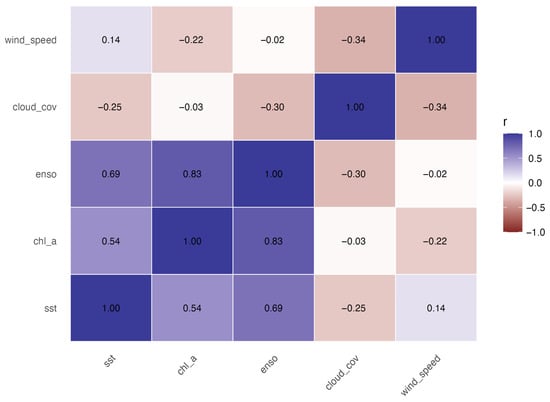
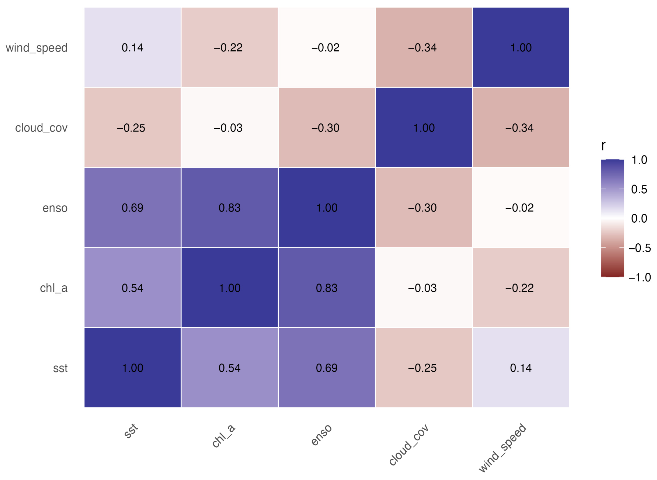
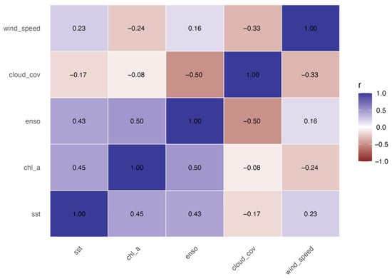
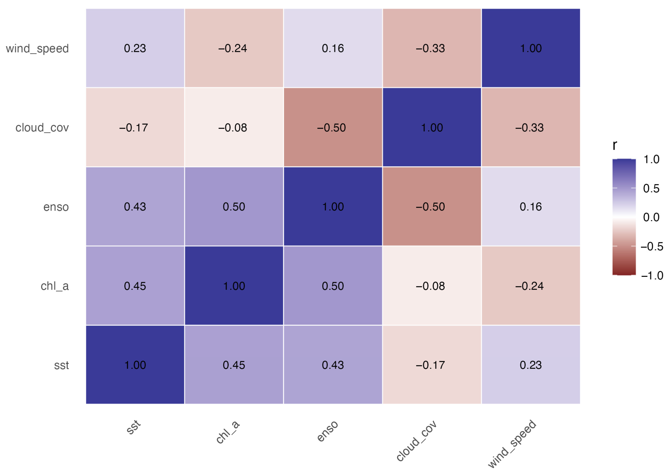
The correlation structure indicates generally moderate associations among the environmental predictors. In the Pearson matrix (Table 7), the largest absolute correlation is observed between enso and chl_a (r = 0.827), which exceeds a conservative screening threshold of $\left|r\right|\ge 0.80$. The next strongest Pearson association is between enso and sst (r = 0.687), followed by chl_a and sst (r = 0.537). All remaining Pearson correlations are small-to-moderate in magnitude. The Spearman matrix (Table 8) corroborates that most dependencies are not extreme; the strongest monotone association is chl_a|enso (r = 0.500), which remains below the r threshold. This discrepancy between Pearson and Spearman for the enso–chl_a pair is consistent with a strong linear component combined with discretization/limited variability in ranks at the available sampling resolution.

Table 7. Pearson correlation matrix among environmental covariates.

	sst	chl_a	enso	cloud_cov	wind_speed
Sst	1.000	0.537	0.687	−0.245	0.144
chl_a	0.537	1.000	0.827	−0.031	−0.224
Enso	0.687	0.827	1.000	−0.301	−0.022
cloud_cov	−0.245	−0.031	−0.301	1.000	−0.344
wind_speed	0.144	−0.224	−0.022	−0.344	1.000

Notes: Pearson r quantifies linear association. Values were computed on complete cases (n = 72).

Table 8. Spearman rank correlation matrix among environmental covariates.

	sst	chl_a	enso	cloud_cov	wind_speed
Sst	1.000	0.453	0.434	−0.167	0.228
chl_a	0.453	1.000	0.500	−0.084	−0.239
Enso	0.434	0.500	1.000	−0.496	0.164
cloud_cov	−0.167	−0.084	−0.496	1.000	−0.325
wind_speed	0.228	−0.239	0.164	−0.325	1.000

Notes: Spearman ρ quantifies monotone association based on ranks. Values were computed on complete cases (n = 72).

VIF diagnostics (Table 9) further suggest that multicollinearity is not severe in the present set of covariates. The largest VIF is observed for enso (VIF = 3.99), followed by chl_a (VIF = 3.28), whereas the remaining covariates show substantially lower values. In combination with the correlation screening, this pattern points to a modest shared signal primarily involving the enso–chl_a pair, without suggesting that the covariate set is dominated by near-linear dependence. Overall, the evidence supports carrying forward the full environmental specification in subsequent models, while treating the enso–chl_a overlap as the main dependency to keep in view when interpreting individual coefficients and when checking the stability of estimates under alternative specifications.

Table 9. Variance inflation factors (VIF) for environmental covariates.

Covariate	VIF
Enso	3.99
chl_a	3.28
sst	1.88
cloud_cov	1.30
wind_speed	1.24

Notes: VIF values below 5 are commonly interpreted as indicating no severe multicollinearity.

The Pearson heatmap (Figure 2) highlights a concentrated block of positive association among sst, chl_a, and enso, with the strongest cell corresponding to the enso–chl_a pair. In contrast, cloud_cov shows weak-to-moderate negative associations with sst and enso, and wind_speed displays only mild correlations overall. The Spearman heatmap (Figure 3) shows a similar qualitative pattern but with attenuated magnitudes, and it more clearly emphasizes the negative monotone relationship between enso and cloud_cov (r $\approx$ −0.50). Overall, the two heatmaps are consistent in indicating that potential collinearity concerns are localized rather than pervasive across the predictor set.

Figure 2. Pearson heatmap.

Figure 3. Spearman heatmap.

3.2.4. PERMANOVA, Multinomial Logistic Regression, Marginal Effects, and Cochran’s Q

Step 1: Results are summarized in Table 10.

Table 10. PERMANOVA results.

Test	Permutations	Strata	df	F	${\mathit{R}}^2$	p_Value	n
PERMANOVA	9999	year	2	0.8436	0.0239	0.6862	72

Notes: The table reports a PERMANOVA (permutational multivariate analysis of variance) testing whether the multivariate environmental conditions differ across the three feeding behaviours (V, P, A). The analysis is based on Euclidean distances computed from the standardized environmental covariates (SST, Chl-a, ENSO, cloud coverage, wind speed) using complete cases (n = 72). Permutations indicate the number of random permutations used to obtain the p-value (9999). Strata = year means permutations were restricted within year blocks to account for inter-annual heterogeneity. The reported F is the pseudo-F statistic, and ${\mathrm{R}}^2$ is the proportion of total multivariate variance explained by behaviour. df refers to the degrees of freedom for the behaviour term. p_value is the permutation-based significance level for the behaviour effect.

The PERMANOVA provides no evidence of behavioural separation in the multivariate environmental space (p = 0.686; Table 10). The explained share of distance variance is small (R² $\approx$ 0.024), indicating that any between-behaviour differences in the joint distribution of the five covariates are modest relative to within-behaviour variability.

Step 2: Multinomial logistic regression and confusion matrix

A multinomial logistic regression was fit to model behaviour as a function of the environmental covariates (and year effects when available). A simple predictive check was performed using an 80/20 random split into training and test sets. Class predictions on the test set were summarized via a confusion matrix and standard metrics (Table 11 and Table 12).

Table 11. Confusion matrix for the multinomial model (test set).

Truth	V	P	A
V	0	1	0
P	0	11	0
A	0	2	1

Notes: The confusion matrix reports out-of-sample classification results for the multinomial logistic model predicting the three feeding behaviours (V, P, A) from the environmental covariates. Rows denote the true observed behaviour in the held-out test set, and columns denote the model’s predicted class (maximum predicted probability). Cell entries are counts of test observations; the diagonal contains correct classifications. The test set size is ${\mathrm{n}}_{\mathrm{t}\mathrm{e}\mathrm{s}\mathrm{t}}=15$ (with ${\mathrm{n}}_{\mathrm{t}\mathrm{r}\mathrm{a}\mathrm{i}\mathrm{n}}=57$ used for model fitting).

Table 12. Predictive diagnostics for the multinomial model (test set).

Metric	Value	n_test	n_train
accuracy	0.8000	15	57
recall_V	0.0000	15	57
recall_P	1.0000	15	57
recall_A	0.3333	15	57
precision_V	NA	15	57
precision_P	0.7857	15	57
precision_A	1.0000	15	57

Notes: Predictive diagnostics are computed from the confusion matrix in Table 10 on the same held-out test set (${\mathrm{n}}_{\mathrm{t}\mathrm{e}\mathrm{s}\mathrm{t}}=15$; ${\mathrm{n}}_{\mathrm{t}\mathrm{r}\mathrm{a}\mathrm{i}\mathrm{n}}=57$). Accuracy is the overall share of correct classifications. Recall (class-specific sensitivity) is the share of correctly predicted observations within each true class (row-wise). Precision (class-specific positive predictive value) is the share of correct predictions among observations predicted as that class (column-wise). Precision for class V is reported as NA because the model never predicted V in the test set (i.e., the predicted-V column total is zero), so the quantity is undefined.

Predictive performance is concentrated in the majority class P: all P observations in the test set were correctly classified (recall_P = 1.00), whereas the minority class V was not recovered (recall_V = 0; Table 11). Classification of A is partial (recall_A $\approx$ 0.33). Precision for V is undefined because no test observation was assigned to V (Table 11). Given the small test sample (n_test = 15) and class imbalance, these diagnostics are best interpreted as a stability check rather than as a definitive assessment of predictive accuracy.

Step 3: Marginal effects on outcome probabilities

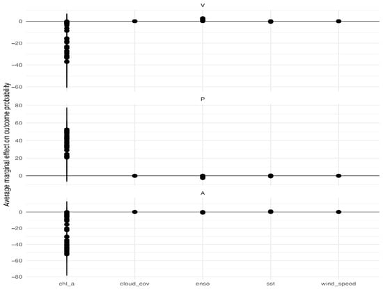
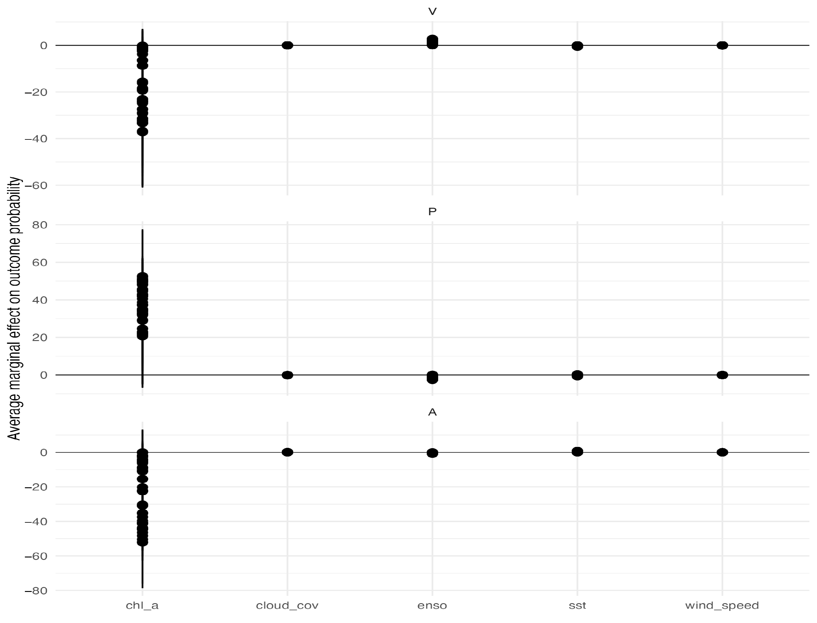
Average marginal effects were computed on the probability scale to summarize how each environmental covariate shifts the predicted probability of each outcome (V, P, A), averaged over the observed covariate distribution. Point estimates and confidence intervals are displayed in Figure 4.

Figure 4. Average marginal effects on outcome probability from the multinomial model (with confidence intervals).

Figure 4 indicates that effects are generally small for most predictors once uncertainty is accounted for, which is coherent with the weak omnibus separation in PERMANOVA (Table 9) and the limited recovery of minority classes in the classification check (Table 11). The most structured pattern is observed for chl_a, which shows outcome-specific shifts consistent with changes in behavioural composition.

Step 4: Cochran’s Q and post hoc McNemar comparisons (A vs. non-A)

A matched-model comparison was performed to assess whether single-covariate logistic models differ in their ability to classify A versus non-A. For each environmental predictor, a separate binomial logistic regression was fit (with year effects when available). Predicted probabilities were thresholded using a prevalence-based cutoff equal to the observed proportion of A in the complete-case sample (cutoff = 0.1944), which is more stable than a 0.5 threshold under class imbalance. For each model and observation, a correctness indicator was defined (1 = correct; 0 = incorrect). Cochran’s Q test was then applied to the matched correctness matrix. Model-wise diagnostics, the Q test, and pairwise McNemar post hoc tests (Holm-adjusted) are reported in Table 13, Table 14 and Table 15.

Table 13. Cochran step diagnostics: model-wise correctness summaries (A vs. non-A).

Model	n_correct	share_correct	var_correct
model_sst	44	0.6111	0.2410
model_chl_a	19	0.2639	0.1970
model_enso	19	0.2639	0.1970
model_cloud_cov	39	0.5417	0.2518
model_wind_speed	41	0.5694	0.2486

Notes: This table summarizes, for each single-covariate logistic model (A vs. non-A), the matched correctness evaluated on the same n = 72 complete-case observations. n_correct is the number of observations correctly classified by the model after converting predicted probabilities to a binary class using the prevalence-based cutoff (cutoff = proportion of A in the analysis sample). share_correct is the corresponding proportion of correct classifications. var_correct is the across-observation variance of the 0/1 correctness indicator.

Table 14. Cochran’s Q test comparing single-covariate models (A vs. non-A).

Test	Q	df	p_Value	n	k_models	cutoff
Cochran Q	47.7500	4	1.064 × 10−9	72	5	0.1944

Notes: This table reports Cochran’s Q test used to assess whether the k = 5 single-covariate models have equal correctness rates for the A vs. non-A classification when evaluated on the same n = 72 observations. Q is the Cochran test statistic, with degrees of freedom df = k_models − 1. p_value quantifies evidence against the null hypothesis that all models perform equally in terms of correctness. cutoff is the prevalence-based probability threshold used to convert predicted probabilities into binary predictions before computing correctness.

Table 15. Pairwise McNemar post hoc tests (Holm-adjusted) for model correctness (A vs. non-A).

Model 1	Model 2	p_Value	p_adj_holm
model_sst	model_chl_a	8.324 × 10−6	8.324 × 10−5
model_sst	model_enso	8.324 × 10−6	8.324 × 10−5
model_chl_a	model_wind_speed	0.000126	0.001008
model_enso	model_wind_speed	0.000126	0.001008
model_chl_a	model_cloud_cov	0.0007829	0.004698
model_enso	model_cloud_cov	0.0007829	0.004698
model_sst	model_cloud_cov	0.4414	1
model_sst	model_wind_speed	0.7003	1
model_chl_a	model_enso	1	1
model_cloud_cov	model_wind_speed	0.8231	1

Notes: This table reports pairwise McNemar post hoc comparisons of classification correctness between single-covariate logistic models for the A vs. non-A contrast. Reported p_value refers to the unadjusted McNemar test, while p_adj_holm is the Holm-adjusted p-value controlling the family-wise error rate across all pairwise comparisons.

Cochran’s Q strongly rejects equality of correctness across the five single-covariate models (Q = 47.75, df = 4, p = 1.06 × ${10}^{-9}$; Table 14), indicating that predictive agreement with the A/non-A contrast differs materially by predictor under the prevalence-based decision rule. Table 13 shows that the sst-only model attains the highest overall correctness (44/72), whereas chl_a-only and enso-only models attain substantially lower correctness (19/72 each). Post hoc McNemar tests (Table 15) support differences between the sst-only model and both chl_a-only and enso-only models after multiplicity adjustment, while differences among sst, cloud_cov, and wind_speed are not supported.

4. Discussion

During the sampling period, 88 individual whale sharks were photo-identified using the I³S Classic programme. This result further confirms that Nosy Be hosts a significant whale shark aggregation, as previously reported by Diamant et al. [5], who photo-identified 681 individuals in this area, highlighting the ecological relevance of this site at a broader spatial scale. Moreover, most of the identified whale sharks were males (n = 37) compared to females (n = 7), and all measured individuals were immature, confirming a sex- and size-based segregation in favour of immature males, as also reported by Diamant et al. [5] for Nosy Be.

However, the high number of unsexed individuals (n = 44), due to observational limitations, constrains robust inference and limits the interpretation of temporal patterns in sex composition. Nonetheless, the overall male bias observed is consistent with previous reports of sex segregation in whale sharks at coastal feeding sites [6,11,19,24,25,33]. Similarly, although the limited number of measured individuals precludes assessments at the scale of the entire aggregation, these observations align with earlier studies showing that coastal aggregation sites are typically dominated by immature individuals [11,19,25,26]. While sex- and size-based segregation are common among shark species—often driven by differences in nutritional requirements or by the avoidance of intra-specific competition and predation—the underlying mechanisms of sexual segregation in whale sharks remain unclear, and dietary differences between immature and mature individuals have been suggested [10].

Our results suggest a decline in whale shark sightings over time in November, from more than 30 individuals observed and photo-identified in 2018 and 2019 to only a few individuals identified in 2022 and 2023. This variability could be likely driven by a combination of environmental conditions, interannual differences in survey effort, and variation in detectability, rather than reflecting true changes in population size, and should therefore be interpreted with caution. The occurrence of whale shark aggregations in the waters surrounding Nosy Be has generally been associated with periods of enhanced productivity [5]. In this region, Pripp et al. [3] identified persistent upwelling activity north of Nosy Be. Unlike classical wind-driven upwelling systems, these processes appear to be primarily associated with a strong north-easterly current linked to an anticyclonic gyre. Previous studies have also suggested that the influence of this gyre in the northern Mozambique Channel may promote localized upwelling along the northern coast of Madagascar [41]. Additional evidence of enhanced productivity was documented by Stephen et al. [42], who reported elevated zooplankton concentrations in localized hotspots near Nosy Be. Furthermore, Pripp et al. [3] recorded large aggregations of seabirds in the area, corroborating the findings of Jaquemet et al. [43], who demonstrated a strong association between seabird distribution and mesoscale eddy activity in the Mozambique Channel. Given the absence of major riverine inputs and the generally low rainfall characterizing the region, terrestrial nutrient supply is likely limited. Consequently, the elevated biological productivity observed in the waters surrounding Nosy Be is most plausibly driven by physical oceanographic processes, particularly upwelling and mesoscale circulation.

Although annual zooplankton biomass concentrations were not directly assessed in this study, it is well established that increased zooplankton availability is closely linked to elevated SSC concentrations [6,30,44]. The data collected indicate a consistent increase in SSC from 2018 to 2019 (0.085 mg/m³) to 2022 (0.125 mg/m³) and 2023 (0.127 mg/m³). While this trend may have promoted higher zooplankton abundance, it did not correspond to an increase in whale shark sightings over time. This discrepancy raises further questions regarding the feeding ecology of whale sharks in Nosy Be, suggesting that they may not rely exclusively on zooplankton and may instead supplement their diet with alternative food sources, as previously proposed by other authors [5,8,17].

To our knowledge, this study represents the first investigation in the waters of Nosy Be specifically aimed at providing preliminary evidence of immature whale shark surface feeding behaviour in relation to environmental variability. More broadly, studies examining the influence of environmental drivers on whale shark surface feeding behaviour remain very scarce [24]. Across the whale-shark sightings, firstly, (i) when the five environmental covariates are considered jointly, the three feeding behaviours (V/P/A) do not occupy clearly distinct environmental conditions: most observations fall in strongly overlapping parts of the multivariate space, and the PERMANOVA indicates that any overall between-behaviour differences are small compared with the variability observed within each behaviour (Table 9). Put differently, very similar combinations of sst, chl-a, enso, cloud_cover, and wind_speed are associated with different feeding behaviours, so the behaviour is unlikely to be explained by a single, stable multivariate set of environmental conditions. (ii) Second, this overlap naturally limits out-of-sample discrimination. In the multinomial logit, the apparent performance is largely a reflection of class prevalence: the model predicts the dominant posture P well but has limited ability to recover the minority postures—especially A—because relatively few A and V events are available to learn stable boundaries (Table 10 and Table 11). Practically, the model is better read as an “association model” than as a reliable classifier of individual events: it captures some structure in the data, but the predictive signal is not strong enough (given the imbalance) to separate rare postures consistently. (iii) Third, the most useful ecological message comes from the marginal effects, which translate the fitted multinomial model into direction-of-change statements for each posture. The marginal effects ask: “holding the rest constant, how does the probability of each feeding posture tend to move when one covariate increases?”. Figure 3 provides this outcome-specific directionality: for each covariate, it summarizes whether the average change in predicted probability is upward or downward for V, P, and A, and how uncertain that average change is. Even when the overall separation between behaviours is limited, marginal effects are still useful because they tell us how the probability of each behaviour tends to change as an environmental variable increases. In other words, the data are not split into clear behavioural ‘zones/clusters’, but some covariates can still shift the balance of observed behaviours (Figure 3). In the marginal-effects analysis, chlorophyll-a (SSC) emerges as the most informative covariate. Its average effects are visibly larger than those of the other predictors and they are consistent across outcomes: increases in SSC are associated with a higher predicted probability of the dominant behaviour P, while the probabilities of V and A tend to decrease on average. Conversely, sst, enso, cloud_cov, and wind_speed exhibit much smaller average effects—typically close to zero relative to ssc—suggesting a more limited contribution to differentiating feeding behaviours in this dataset.

The results indicate that SSC concentration was the most influential environmental variable associated with immature whale shark surface feeding behaviour, and that under elevated SSC conditions, P feeding was significantly more prevalent and V and A tend to decrease. Areas characterized by higher SSC concentrations generally reflect increased prey availability, which “normally” may favour A and vertical V feeding strategies [21,24,45,46]. Conversely, lower SSC concentrations are typically associated with reduced prey densities, under which P feeding behaviour tends to predominate [24,46]. V feeding allows whale sharks to ingest large quantities of prey over short time intervals without forward movement, which may be energetically advantageous when prey is densely aggregated [22]. Given the large body size and associated energetic demands of whale sharks, reliance on dense prey patches is likely necessary to meet daily metabolic requirements. Other factors not considered in this study could explain why P is the overall prevalent behaviour, perhaps linked to zooplankton ecology. The work by Bava et al. 2022 [8] highlighted the presence of size classes and annual fluctuations in its abundance, with a lower abundance in 2019 compared to 2018, with a decrease in Copepoda and Cnidaria in favour of Appendicularia. However, although SSC concentrations in 2018 and 2019 were lower than those recorded in 2022 and 2023—supporting the higher frequency of P feeding behaviour observed in those earlier years—in 2023 SSC reached its highest recorded value, yet P feeding remained the most frequently displayed strategy. The lack of a consistent correspondence between increasing SSC concentrations and the expected dominant feeding strategy suggests that SSC alone may not fully capture the environmental conditions governing immature whale shark surface feeding behaviour, and that additional parameters should be considered. Although sampling campaigns coincided with the onset of the rainy season, average rainfall during fieldwork periods was low (<2 mm/h¹), indicating limited terrestrial nutrient input at the time of surveys. Consequently, short-term variability in prey availability is unlikely to have been strongly influenced by riverine nutrient inputs. At the same time, large-scale climatic drivers, including variations in air temperature and SST, may influence water quality and ecosystem functioning. Changes in precipitation regimes can affect nutrient transport from land, while increasing temperatures may alter biogeochemical cycling, primary productivity, microbial processes, evapotranspiration, and water-column stratification [47]. Taken together, these interacting processes may contribute to variability in prey distribution and availability that is not fully captured by SSC concentrations alone.

The significance of ENSO—the largest VIF is observed for enso (VIF = 3.99), followed by chl_a (VIF = 3.28), whereas the remaining covariates show substantially lower values— is interesting. In combination with the correlation screening, this pattern points to a modest shared signal primarily involving the enso–sst pair, without suggesting that the covariate set is dominated by near-linear dependence. Overall, the evidence supports carrying forward the full environmental specification in subsequent models, while treating the enso–chl_a overlap as the main dependency to keep in view when interpreting individual coefficients and when checking the stability of estimates under alternative specifications. In the southwestern Indian Ocean, ENSO phases are closely linked to other climatic and oceanographic processes, including tropical cyclone activity and dipole systems [48].

V feeding was most frequently observed in 2022, coinciding with a strong La Niña event (MEI = −1.3), conditions typically associated with increased cyclone activity, higher rainfall, and stronger winds, which enhance water-column mixing and promote localized prey aggregation [24]. In contrast, 2023 coincided with a strong El Niño event (MEI = 1.1), while 2018 and 2019 coincided with moderate El Niño conditions (MEI = 0.1 in 2018 and MEI = 0.4 in 2019). During these periods, reduced cyclone activity and weaker wind forcing likely limited mixing, resulting in lower prey aggregation and a predominance of P feeding behaviour [24]. SST and wind speed were not retained in the final models. Whale sharks exhibit broad thermal tolerance and commonly occupy near-surface waters within a relatively narrow temperature range [28], which may explain the absence of a detectable SST effect on surface feeding behaviour in this study. Similarly, wind speeds recorded during the study period were generally low and likely insufficient to generate substantial mixing capable of influencing nutrient redistribution or prey aggregation, thereby limiting their observable effect on surface feeding behaviour [49].

5. Conclusions

Investigating the effects of environmental factors on whale shark surface feeding behaviour remains inherently challenging due to the complex and dynamic nature of marine ecosystems and the high variability of environmental drivers. Nevertheless, these preliminary findings, in line with recent studies, suggest that variables such as SSC concentration, and ENSO, even if they do not appear to provide a strong enough predictive signal of feeding behaviours, can instead provide the probability of a certain type of behaviour in the presence of an increase in one of the environmental variables.

Despite these preliminary insights, further research incorporating direct measures of phytoplankton and zooplankton abundance over longer temporal scales integrated with data on the prey subject to feeding behaviour is required to better characterize prey availability and its relationship with surface feeding strategies of immature whale sharks, as well as improve other environmental variables not analyzed in the present study. Improving the ability to predict whale shark surface feeding behaviour based on environmental parameters may enhance our understanding of habitat use and spatial distribution in the study area, particularly given the species’ sensitivity to fluctuations in food resources. Moreover, the potential influence of global climate change on whale shark feeding ecology warrants careful consideration. Consequently, long-term and continuous data collection is essential to disentangle the relative roles of local and regional drivers and to provide robust information to support effective management and conservation of whale sharks in this area of high ecological and conservation value.

References

- Diamant, S.; Rohner, C.A.; Kiszka, J.J.; Guillemain, A.; Guillemain, T.; Sourisseau, E.; Pierce, S.J. Movements and Habitat Use of Satellite-Tagged Whale Sharks off Western Madagascar. Endanger. Species Res. 2018, 36, 49–58. [Google Scholar] [CrossRef] [Scilit]
- Malauene, B.S.; Shillington, F.A.; Roberts, M.J.; Moloney, C.L. Cool, Elevated Chlorophyll-a Waters off Northern Mozambique. Deep Sea Res. Part II Top. Stud. Oceanogr. 2014, 100, 68–78. [Google Scholar] [CrossRef] [Scilit]
- Pripp, T.; Gammelsrød, T.; Krakstad, J.O. Physical Influence on Biological Production along the Western Shelf of Madagascar. Deep. Sea Res. Part II Top. Stud. Oceanogr. 2014, 100, 174–183. [Google Scholar] [CrossRef] [Scilit]
- Ziegler, J.A.; Diamant, S.; Pierce, S.J.; Bennett, R.; Kiszka, J.J. Economic value and public perceptions of whale shark tourism in nosy be, madagascar. Tour. Mar. Environ. 2021, 16, 167–182. [Google Scholar] [CrossRef] [Scilit]
- Diamant, S.; Pierce, S.J.; Rohner, C.A.; Graham, R.T.; Guillemain d’Echon, A.; Guillemain d’Echon, T.; Sourisseau, E.; Fidiarisandratra, L.C.; Bakary, G.; Trélanche, S.; et al. Population Structure, Residency, and Abundance of Whale Sharks in the Coastal Waters off Nosy Be, North-Western Madagascar. Aquat. Conserv. Mar. Freshw. Ecosyst. 2021, 31, 3492–3506. [Google Scholar] [CrossRef] [Scilit]
- Boldrocchi, G.; Omar, M.; Azzola, A.; Bettinetti, R. The Ecology of the Whale Shark in Djibouti. Aquat. Ecol. 2020, 54, 535–551. [Google Scholar] [CrossRef] [Scilit]
- Ketchum, J.T.; Galván-Magaña, F.; Klimley, A.P. Segregation and Foraging Ecology of Whale Sharks, Rhincodon typus, in the Southwestern Gulf of California. Environ. Biol. Fishes 2013, 96, 779–795. [Google Scholar] [CrossRef] [Scilit]
- Bava, P.; Micarelli, P.; Buttino, I. Zooplankton Assemblage Diversity in the Whale Shark Rhincodon typus Aggregation Area of Nosy Be (Madagascar). Estuar. Coast. Shelf Sci. 2022, 279, 108159. [Google Scholar] [CrossRef] [Scilit]
- Rohner, C.A.; Couturier, L.I.E.; Richardson, A.J.; Pierce, S.J.; Prebble, C.E.M.; Gibbons, M.J.; Nichols, P.D. Diet of Whale Sharks Rhincodon typus Inferred from Stomach Content and Signature Fatty Acid Analyses. Mar. Ecol. Prog. Ser. 2013, 493, 219–235. [Google Scholar] [CrossRef] [Scilit]
- Rohner, C.A.; Armstrong, A.J.; Pierce, S.J.; Prebble, C.E.M.; Cagua, E.F.; Cochran, J.E.M.; Berumen, M.L.; Richardson, A.J. Whale Sharks Target Dense Prey Patches of Sergestid Shrimp off Tanzania. J. Plankton Res. 2015, 37, 352–362. [Google Scholar] [CrossRef] [Scilit]
- Meekan, M.G.; Jarman, S.N.; Mclean, C.; Schultz, M.B. DNA Evidence of Whale Sharks (Rhincodon typus) Feeding on Red Crab (Gecarcoidea natalis) Larvae at Christmas Island, Australia. Mar. Freshw. Res. 2009, 60, 607–609. [Google Scholar] [CrossRef] [Scilit]
- Sampaio, C.L.S.; Leite, L.; Reis-filho, J.A.; Loiola, M.; Miranda, R.J.; Nunes, J.d.A.C.; Macena, B.C.L. New Insights into Whale Shark Rhincodon typus Diet in Brazil: An Observation of Ram Filter-Feeding on Crab Larvae and Analysis of Stomach Contents from the First Stranding in Bahia State. Environ. Biol. Fishes 2018, 101, 1285–1293. [Google Scholar] [CrossRef] [Scilit]
- de la Parra Venegas, R.; Hueter, R.; Cano, J.G.; Tyminski, J.; Remolina, J.G.; Maslanka, M.; Ormos, A.; Weigt, L.; Carlson, B.; Dove, A. An Unprecedented Aggregation of Whale Sharks, Rhincodon typus, in Mexican Coastal Waters of the Caribbean Sea. PLoS ONE 2011, 6, e18994. [Google Scholar] [CrossRef] [Scilit] [PubMed]
- Robinson, D.P.; Jaidah, M.Y.; Jabado, R.W.; Lee-Brooks, K.; Nour El-Din, N.M.; Malki, A.A.A.; Elmeer, K.; McCormick, P.A.; Henderson, A.C.; Pierce, S.J.; et al. Whale Sharks, Rhincodon typus, Aggregate around Offshore Platforms in Qatari Waters of the Arabian Gulf to Feed on Fish Spawn. PLoS ONE 2013, 8, e58255. [Google Scholar] [CrossRef] [Scilit]
- Fox, S.; Foisy, I.; De La Parra Venegas, R.; Galván Pastoriza, B.E.; Graham, R.T.; Hoffmayer, E.R.; Holmberg, J.; Pierce, S.J. Population Structure and Residency of Whale Sharks Rhincodon typus at Utila, Bay Islands, Honduras. J. Fish Biol. 2013, 83, 574–587. [Google Scholar] [CrossRef] [Scilit]
- Boldrocchi, G.; Bettinetti, R. Whale Shark Foraging on Baitfish off Djibouti. Mar. Biodivers. 2019, 49, 2013–2016. [Google Scholar] [CrossRef] [Scilit]
- Marsili, L.; Consales, G.; Romano, P.; Rosai, R.; Bava, P.; Reinero, F.R.; Micarelli, P. A Cocktail of Plankton and Organochlorines for Whale Shark in the Foraging Areas of Nosy Be (Madagascar). Diversity 2023, 15, 911. [Google Scholar] [CrossRef] [Scilit]
- Whitehead, D.A.; Gayford, J. First Record of Bottom-Feeding Behaviour in the Whale Shark (Rhincodon typus). J. Fish Biol. 2023, 103, 448–452. [Google Scholar] [CrossRef] [Scilit]
- Rowat, D.; Brooks, K.S. A Review of the Biology, Fisheries and Conservation of the Whale Shark Rhincodon typus. J. Fish Biol. 2012, 80, 1019–1056. [Google Scholar] [CrossRef] [Scilit] [PubMed]
- Clark, E. Whale Sharks: Gentle Monsters of the Deep. Natl. Geogr. 1992, 182, 123–138. [Google Scholar]
- Cade, D.E.; Levenson, J.J.; Cooper, R.; de la Parra, R.; Webb, D.H.; Dove, A.D.M. Whale Sharks Increase Swimming Effort While Filter Feeding, but Appear to Maintain High Foraging Efficiencies. J. Exp. Biol. 2020, 223, jeb224402. [Google Scholar] [CrossRef] [Scilit]
- Nelson, J.D.; Eckert, S.A. Foraging Ecology of Whale Sharks (Rhincodon typus) within Bahía de Los Angeles, Baja California Norte, México. Fish. Res. 2007, 84, 47–64. [Google Scholar] [CrossRef] [Scilit]
- Montero-Quintana, A.N.; Ocampo-Valdez, C.F.; Vázquez-Haikin, J.A.; Sosa-Nishizaki, O.; Osorio-Beristain, M. Whale Shark (Rhincodon typus) Predatory Flexible Feeding Behaviors on Schooling Fish. J. Ethol. 2021, 39, 399–410. [Google Scholar] [CrossRef] [Scilit]
- Reinero, F.R.; Marsella, A.; Pacifico, A.; Vicariotto, C.; Maule, L.; Mahrer, M.; Micarelli, P. Influence of Environmental Factors on the Surface Feeding Behaviour of Immature Male Whale Sharks in the Gulf of Tadjoura (Djibouti). Conservation 2024, 4, 792–811. [Google Scholar] [CrossRef] [Scilit]
- Rowat, D.; Gore, M.; Meekan, M.G.; Lawler, I.R.; Bradshaw, C.J.A. Aerial Survey as a Tool to Estimate Whale Shark Abundance Trends. J. Exp. Mar. Biol. Ecol. 2009, 368, 1–8. [Google Scholar] [CrossRef] [Scilit]
- Araujo, G.; Lucey, A.; Labaja, J.; So, C.L.; Snow, S.; Ponzo, A. Population Structure and Residency Patterns of Whale Sharks, Rhincodon typus, at a Provisioning Site in Cebu, Philippines. PeerJ 2014, 2, e543. [Google Scholar] [CrossRef] [Scilit]
- Hacohen-Domené, A.; Martínez-Rincón, R.O.; Galván-Magaña, F.; Cárdenas-Palomo, N.; de la Parra-Venegas, R.; Galván-Pastoriza, B.; Dove, A.D.M. Habitat Suitability and Environmental Factors Affecting Whale Shark (Rhincodon typus) Aggregations in the Mexican Caribbean. Environ. Biol. Fishes 2015, 98, 1953–1964. [Google Scholar] [CrossRef] [Scilit]
- Sequeira, A.; Mellin, C.; Rowat, D.; Meekan, M.G.; Bradshaw, C.J.A. Ocean-Scale Prediction of Whale Shark Distribution. Divers. Distrib. 2012, 18, 504–518. [Google Scholar] [CrossRef] [Scilit]
- Sequeira, A.M.M.; Mellin, C.; Fordham, D.A.; Meekan, M.G.; Bradshaw, C.J.A. Predicting Current and Future Global Distributions of Whale Sharks. Glob. Change Biol. 2014, 20, 778–789. [Google Scholar] [CrossRef] [Scilit]
- Sleeman, J.C.; Meekan, M.G.; Wilson, S.G.; Polovina, J.J.; Stevens, J.D.; Boggs, G.S.; Bradshaw, C.J.A. To Go or Not to Go with the Flow: Environmental Influences on Whale Shark Movement Patterns. J. Exp. Mar. Biol. Ecol. 2010, 390, 84–98. [Google Scholar] [CrossRef] [Scilit]
- Ranintyari, M.; Sunarto; Syamsuddin, M.L.; Astuty, S. Effects of Oceanographic Factors on Spatial Distribution of Whale Shark in Cendrawasih Bay Effects of Oceanographic Factors on Spatial Distribution of Whale Shark in Cendrawasih Bay National Park, West Papua. IOP Conf. Ser. Earth Environ. Sci. 2017, 149, 012050. [Google Scholar] [CrossRef] [Scilit]
- Manuhutu, J.F.; Wiadnya, D.G.R.; Sambah, A.B.; Herawati, E.Y. The Presence of Whale Sharks Based on Oceanographic Variations in Cenderawasih Bay National Park, Papua, Indonesia. Biodiversitas J. Biol. Divers. 2021, 22, 4948–4955. [Google Scholar] [CrossRef] [Scilit]
- Reinero, F.R.; Marsella, A.; Vitale, G.; Pacifico, A.; Mahrer, M.; Micarelli, P. Environmental Drivers of Immature Whale Shark Surface Sightings in the Gulf of Tadjoura, Djibouti. Conservation 2025, 5, 68. [Google Scholar] [CrossRef] [Scilit]
- Motta, P.J.; Maslanka, M.; Hueter, R.E.; Davis, R.L.; de la Parra, R.; Mulvany, S.L.; Habegger, M.L.; Strother, J.A.; Mara, K.R.; Gardiner, J.M.; et al. Feeding Anatomy, Filter-Feeding Rate, and Diet of Whale Sharks Rhincodon typus during Surface Ram Filter Feeding off the Yucatan Peninsula, Mexico. Zoology 2010, 113, 199–212. [Google Scholar] [CrossRef] [Scilit]
- Gleiss, A.C.; Wright, S.; Liebsch, N.; Wilson, R.P.; Norman, B. Contrasting Diel Patterns in Vertical Movement and Locomotor Activity of Whale Sharks at Ningaloo Reef. Mar. Biol. 2013, 160, 2981–2992. [Google Scholar] [CrossRef] [Scilit]
- Catlin, J.; Jones, R. Whale Shark Tourism at Ningaloo Marine Park: A Longitudinal Study of Wildlife Tourism. Tour. Manag. 2010, 31, 386–394. [Google Scholar] [CrossRef] [Scilit]
- Arzoumanian, Z.; Holmberg, J.; Norman, B. An Astronomical Pattern-Matching Algorithm for Computer-Aided Identification of Whale Sharks Rhincodon typus. J. Appl. Ecol. 2005, 42, 999–1011. [Google Scholar] [CrossRef] [Scilit]
- Matsumoto, R.; Toda, M.; Matsumoto, Y.; Ueda, K.; Nakazato, M.; Sato, K.; Uchida, S. Notes on Husbandry of Whale Sharks, Rhincodon typus, in Aquaria. In Elasmobranch Husbandry Manual II: Recent Advances in the Care of Sharks, Rays and their Relatives; Special Publication of the Ohio Biological Survey; Ohio Biological Survey: Hilliard, OH, USA, 2017; pp. 15–22. [Google Scholar]
- Kyba, C.C.M.; Ruhtz, T.; Fischer, J.; Hölker, F. Cloud Coverage Acts as an Amplifier for Ecological Light Pollution in Urban Ecosystems. PLoS ONE 2011, 6, e17307. [Google Scholar] [CrossRef] [Scilit]
- Pierce, S.J.; Pardo, S.A.; Rohner, C.A.; Matsumoto, R.; Murakumo, K.; Nozu, R.; Dove, A.D.M.; Perry, C.; Meekan, M.G. Whale Shark Reproduction, Growth, and Demography. In Whale Sharks: Biology, Ecology and Conservation; Dove, A.D.M., Pierce, S.J., Eds.; CRC Press: Boca Raton, FL, USA, 2021; pp. 13–46. [Google Scholar]
- Payet, R.A.; Soogun, N.; Ranaivoson, E.; Payet, R.J.; Ali Abdallah, F. Global International Waters Assessment Indian Ocean Islands. In GIWA Regional Assessment 45b; UNEP: Nairobi, Kenya; GEF: Washington, DC, USA; University of Kalmar: Kalmar, Sweden, 2004; p. 175. ISBN 1651-9402. [Google Scholar]
- Stephen, R.; Saraladevi, K.; Meenakshikunjamma, P.P.; Gopalakrishnan, T.C.; Saraswathy, M. Calanoid Copepods of the International Indian Ocean Expedition Collections. In Oceanography of the Indian Ocean; Desai, B.N., Ed.; Oxford & IBH Publishing: New Delhi, India, 1992; pp. 143–156. [Google Scholar]
- Jaquemet, S.; Ternon, J.F.; Kaehler, S.; Thiebot, J.B.; Dyer, B.; Bemanaja, E.; Marteau, C.; Le Corre, M. Contrasted Structuring Effects of Mesoscale Features on the Seabird Community in the Mozambique Channel. Deep Sea Res. Part II Top. Stud. Oceanogr. 2014, 100, 200–211. [Google Scholar] [CrossRef] [Scilit]
- Hsu, H.H.; Joung, S.J.; Liao, Y.Y.; Liu, K.M. Satellite Tracking of Juvenile Whale Sharks, Rhincodon typus, in the Northwestern Pacific. Fish. Res. 2007, 84, 25–31. [Google Scholar] [CrossRef] [Scilit]
- Colman, J.G. A Review of the Biology and Ecology of the Whale Shark. J. Fish Biol. 1997, 51, 1219–1234. [Google Scholar] [CrossRef]
- Whitehead, D.A.; Jakes-Cota, U.; Pancaldi, F.; Galván-Magaña, F.; Gonzalez-Armas, R. The Influence of Zooplankton Communities on the Feeding Behavior of Whale Shark in Bahia de La Paz, Gulf of California. Rev. Mex. Biodivers. 2020, 91, 1–8. [Google Scholar] [CrossRef] [Scilit]
- Coffey, R.; Paul, M.J.; Stamp, J.; Hamilton, A.; Johnson, T. A Review of Water Quality Responses to Air Temperature and Precipitation Changes 2: Nutrients, Algal Blooms, Sediment, Pathogens. JAWRA J. Am. Water Resour. Assoc. 2019, 55, 844–868. [Google Scholar] [CrossRef] [Scilit] [PubMed]
- Sagita, N.; Takemi, T. Influences of Indian Ocean Dipole and El Niño–Southern Oscillation on Thunderstorm Events in Indonesia. Int. J. Climatol. 2025, 45, e8931. [Google Scholar] [CrossRef] [Scilit]
- Krasheninnikova, S.B.; Chmyr, V.D.; Lee, R.I.; Minkina, N.I. Long-Term Dynamics of Phytoplankton Parameters and Water Temperature in the Area of Sevastopol (Black Sea). Oceanology 2024, 64, 391–401. [Google Scholar] [CrossRef] [Scilit]
Disclaimer/Publisher’s Note: The statements, opinions and data contained in all publications are solely those of the individual author(s) and contributor(s) and not of MDPI and/or the editor(s). MDPI and/or the editor(s) disclaim responsibility for any injury to people or property resulting from any ideas, methods, instructions or products referred to in the content. |
© 2026 by the authors. Licensee MDPI, Basel, Switzerland. This article is an open access article distributed under the terms and conditions of the Creative Commons Attribution (CC BY) license.