


Abstract
Alpine grassland ecosystems are increasingly exposed to global change and human activities, yet their long-term resilience dynamics, stagewise shifts, and nonlinear driver associations remain unclear in northwestern Sichuan, China. We estimated a grassland resilience index (RI) for 1985–2020 using a first-order autoregressive model within centered five-year moving windows. Inputs comprised monthly normalized difference vegetation index (NDVI), temperature, and precipitation data for 1983–2022. Exploratory change-pattern analysis, nested group cross-validation, Shapley Additive exPlanations (SHAP), and accumulated local effects (ALE) characterized temporal changes and predictor associations. Regional RI declined significantly under autocorrelation-adjusted inference. Exploratory classification assigned 54.01% of grassland to linear or candidate turning patterns; 75.56% of candidate turning areas showed increase-to-decrease patterns. Random forest achieved a mean outer-test R2 of 0.36 ± 0.02, decreasing to 0.24 ± 0.05 under 100 km spatial-block validation and 0.11 ± 0.02 without Year. Year accounted for 48.68% of full-model SHAP importance. Among the seven ecological predictors, temperature–energy factors contributed 51.96%, exceeding moisture-related factors (35.51%). However, this dominance was not robust to excluding Year (driver-rank Spearman ρ = −0.29). ALE revealed asymmetric temperature associations, whereas grazing responses varied across periods. These results indicate limited predictive power of ecological predictors alone and Year-sensitive driver attribution.
1. Introduction
Global change is continually altering the structure, functioning, and stability of terrestrial ecosystems [1]. Holling first introduced resilience into ecology in 1973, emphasizing the capacity of ecosystems to absorb disturbances while maintaining their basic structure and function [2]. Classical theory distinguishes ecological resilience, the capacity to absorb disturbance without a state shift, from engineering resilience, the rate of return to a previous state [3]. The time-series metric used here mainly represents post-disturbance recovery rate and is therefore operationally closer to engineering resilience. Here, resilience denotes recovery capacity after disturbance; resistance denotes the capacity to persist during disturbance; temporal stability describes temporal variability in system state; and vulnerability denotes susceptibility to external stress. Resilience has consequently become central to research on climate-change impacts, adaptation, and risk [4]. Grasslands provide carbon storage, water regulation, biodiversity conservation, and pastoral production, but are sensitive to climatic change and human use [5]. Since the 1980s, regional divergence in global grassland biomass change has widened, demonstrating strong spatial heterogeneity in productivity responses to global change [6]. Alpine grasslands on the Qinghai–Tibet Plateau are jointly constrained by low temperature, water availability, freeze–thaw processes, and short growing seasons; the influence of long-term warming on productivity stability is time-dependent [7]. Mountain grasslands also provide habitats for diverse species and play an important role in biodiversity conservation [5]. Alpine grasslands in northwestern Sichuan support water conservation and pastoral production and exhibit pronounced spatial heterogeneity in aboveground biomass and ecosystem resilience [8]. These characteristics make the region a representative setting for examining long-term changes in recovery capacity.
Recent resilience research has progressed from conceptual discussion to quantitative assessment based on long-term Earth observations. Recovery rates and temporal autocorrelation have been used to characterize ecosystem recovery dynamics. According to critical-slowing-down theory, slower recovery from small perturbations may be accompanied by increased temporal autocorrelation [9,10]. Remote-sensing studies have further applied temporal autocorrelation to assess vegetation resilience [11]. Interpreting these indicators assumes relatively small perturbations and approximately stationary dynamics within local analysis windows. Temporal trends and seasonal cycles also require careful consideration [9,10]. Lenton et al. cautioned that declining resilience inferred from remote-sensing time series does not necessarily indicate that an ecosystem has crossed a critical threshold. Its ecological meaning depends on the processes and scales considered [12]. Yao et al. further reported a dynamic trade-off between resistance and resilience, indicating that stability dimensions do not represent identical processes [13]. Studies of drivers have often emphasized moisture availability and variability. Global vegetation resilience is closely associated with water availability and interannual variability, and water limitation can weaken recovery capacity [14]. Long-term changes in global grassland growth peaks may also be affected by decadal drought disturbances [15], while grassland resilience in China declines with greater interannual precipitation variability [16]. Existing research has therefore focused primarily on overall resilience trends and the roles of moisture conditions and variability. However, the relative importance of temperature and energy inputs remains insufficiently tested in alpine grasslands with strong thermal limitation and pronounced hydrothermal heterogeneity. Systematic characterization of interannual fluctuations, temporal turning points, and nonlinear driver responses is also limited.
Alpine grasslands on the Qinghai–Tibet Plateau are sensitive to climate change and human activities, and their changes and adaptive-management needs vary substantially among regions [17,18]. Long-term studies have identified threshold effects of grazing intensity [19], potential degradation thresholds using early-warning signals such as spatial and temporal autocorrelation [20], and an overall, accelerating decline in Tibetan Plateau vegetation resilience [21]. Moderate grazing may promote compensatory plant growth in alpine meadows under certain conditions [22]. In contrast, heavy grazing may reduce vegetation productivity and degrade soil properties [23]. These contrasting responses provide a plausible ecological basis for expecting a non-monotonic association between grazing intensity and grassland recovery capacity. Northwestern Sichuan lies on the eastern margin of the plateau, where complex topography produces strong hydrothermal heterogeneity [24] and may modify the relative roles of water and thermal limitations. Whether plateau-scale resilience patterns and grazing thresholds apply locally therefore needs further testing. Existing work in northwestern Sichuan has mainly examined ecological vulnerability and highlighted the roles of shallow soil moisture and grazing intensity [25,26]. Vulnerability, however, integrates exposure, sensitivity, and resilience, whereas the present RI primarily represents post-disturbance recovery rate. The spatial patterns and dominant controls of these two properties need not coincide. Long-term grassland resilience and its drivers in northwestern Sichuan therefore warrant a dedicated assessment.
Northwestern Sichuan, located on the eastern margin of the Qinghai–Tibet Plateau and in the headwaters of the Yangtze and Yellow Rivers, is an important water-conservation area and alpine ecological barrier [27]. Clarifying long-term changes, temporal turning points, and drivers of grassland resilience under climatic change and grazing disturbance can contribute to understanding regional ecosystem stability [7,17]. We tested three hypotheses. H1: we expected the regional grassland resilience index (RI) to decline overall during 1985–2020, with spatially varying temporal turning points. This expectation reflects the potential for climatic variability and grazing disturbance to weaken recovery capacity differently across the region. H2: we expected temperature–energy factors to show stronger associations with RI than moisture-related factors under strong thermal limitation. We also expected asymmetric nonlinear responses to maximum temperature (TMX) and minimum temperature (TMN). H3: we expected grazing intensity (GI) to exhibit a non-monotonic association with RI, with potentially negative associations at high grazing-intensity levels.
To test these hypotheses, we used monthly normalized difference vegetation index (NDVI), temperature, and precipitation data for 1983–2022 to construct a 1985–2020 grassland RI series with five-year centered moving windows. Long-term change, variability, and temporal turning points were assessed at regional and pixel scales to test H1. At the 20 km × 20 km grid scale, candidate models were compared using nested group cross-validation. Shapley Additive exPlanations (SHAP) and accumulated local effects (ALE) were then used to interpret the final model and examine key drivers and nonlinear responses, testing H2 and H3. This study contributes by: (1) constructing a long-term, pixel-level RI series for northwestern Sichuan grasslands and mapping its changes and turning points; (2) improving the robustness of driver attribution through multi-model comparison under nested group cross-validation; and (3) characterizing asymmetric temperature associations and an intensity-dependent grazing response to inform adaptive grassland management under climate change and grazing disturbance.
2. Materials and Methods
The workflow comprised four components: data preprocessing, construction of the grassland RI, regional- and pixel-scale change analyses, and driver analysis and interpretation (Figure 1). Details are provided in Section 2.3.1, Section 2.3.2 and Section 2.3.3.
Figure 1.
Research framework.
2.1. Study Area
The northwestern Sichuan grassland ecosystem (NSGE; 27°56′–34°20′ N, 97°21′–104°27′ E) is located on the eastern margin of the Qinghai–Tibet Plateau and includes the Ganzi Tibetan Autonomous Prefecture and the Ngawa Tibetan and Qiang Autonomous Prefecture. The region has pronounced topographic relief, with grasslands extending from approximately 784 to 6448 m a.s.l. (Figure 2a). The grasslands cover about 143,600 km2 and are dominated by alpine meadow (72.36%) and temperate mountain meadow (25.96%) (Figure 2b). High elevation and complex terrain create marked spatial hydrothermal contrasts. Mean annual temperature ranges from approximately −20 to 16 °C (Figure 2c), while mean annual precipitation ranges from 475 to 1018 mm (Figure 2d). Extensive pastoral activity, together with complex terrain and hydrothermal gradients, makes the NSGE a representative region for examining long-term resilience dynamics, temporal turning points, and their drivers [28].
Figure 2.
Overview of the northwestern Sichuan grassland ecosystem (NSGE). (a) Elevation; (b) grassland types (AM, alpine meadow; TMM, temperate mountain meadow; LSM, lowland saline meadow; Marsh, marsh); (c) mean annual temperature; and (d) mean annual precipitation.
2.2. Data Sources and Preprocessing
We used multi-source data on grassland extent, elevation, vegetation, climate and moisture, and human activities. Variable names, abbreviations, spatial and temporal resolutions, and coverage are listed in Table 1; sources and preprocessing are described below.
Table 1.
Basic information on the main data used in this study.
Grassland extent was derived from the 1:1,000,000 China Grassland Resource Map compiled by Su [29]. The historical grassland extent was used as a fixed spatial mask throughout 1985–2020 to maintain a consistent reference area for temporal comparisons. Accordingly, RI trends and area proportions were evaluated for valid pixels within this baseline grassland extent, without explicitly accounting for changes in land-cover categories over time. Elevation (ELE) was obtained from the 500 m digital elevation model of the Resource and Environmental Science Data Platform (https://www.resdc.cn/data.aspx?DATAID=123, accessed on 15 January 2025) [30,31]. NDVI was obtained from the Peking University GIMMS NDVI product (https://zenodo.org/records/8253971, accessed on 15 January 2025) [32], whose long coverage and cross-sensor calibration support long-term grassland analysis. Mean temperature (TEM), maximum temperature (TMX), minimum temperature (TMN), and precipitation (PRE) were obtained from the 1 km monthly temperature and precipitation dataset for China released by the National Earth System Science Data Center (https://www.geodata.cn/ accessed on 15 January 2025) [33]. Solar radiation (SR) was obtained from the Geographic Remote Sensing Ecological Network Platform (https://www.gisrs.cn/ accessed on 15 January 2025) [34,35]. Potential evapotranspiration (PET), actual evapotranspiration (AET), soil moisture (SM), and vapor pressure deficit (VPD) were obtained from TerraClimate (https://www.climatologylab.org/terraclimate.html, accessed on 15 July 2025) [36]. Relative humidity (RHU) was obtained from the ChinaMet high-resolution meteorological forcing dataset of the National Cryosphere Desert Data Center (https://www.ncdc.ac.cn/ accessed on 15 January 2025) [37,38,39]. Aridity index (AI) was obtained from the National Earth System Science Data Center [33,40,41,42]. Grazing intensity (GI) was obtained from the National Ecosystem Science Data Center [43]. Artificial nighttime light (NTL) was obtained from the National Tibetan Plateau Data Center [44,45].
To reduce differences in coordinate reference systems, temporal scales, and spatial resolutions, all rasters were preprocessed consistently. Spatially, data were projected to WGS 1984, clipped, screened for invalid values, and aligned; nearest-neighbor resampling was used to harmonize grid alignment. Area calculation, spatial aggregation, and regular-grid construction used a projected coordinate system in metres. Temporally, 15-day NDVI was aggregated to monthly values by maximum-value compositing (MVC). TEM, TMX, TMN, SM, VPD, PRE, SR, PET, and AET were aggregated to annual values; RHU, AI, GI, and NTL, originally supplied at annual resolution, were used directly. Missing model inputs were imputed with medians estimated solely from the training folds and then applied to the corresponding validation and test folds to prevent leakage.
Spatially, all drivers were resampled to 1 km × 1 km and overlaid with the grassland mask. Resampling was used only to harmonize grid alignment and pixel size and did not add spatial information; accordingly, the NDVI-based RI remained constrained by the original approximately 8 km spatial resolution. Nearest-neighbor resampling did not create additional independent NDVI observations; therefore, the harmonized 1 km raster cells were not considered independent spatial samples. Given the scale dependence of ecological processes and their driver relationships [46,47,48], we compared effective grassland areas within 10 km × 10 km and 20 km × 20 km grids. At the 10 km scale, the lower quartile and median effective grassland areas were 31.04 and 55.13 km2, respectively, both below or close to the approximately 64 km2 area of an original 8 km RI pixel. At the 20 km scale, the corresponding values were 105.02 and 201.40 km2, indicating that spatial support was relatively limited in some 10 km grids. Considering the original data scale, the stability of grid statistics, and the need to retain spatial heterogeneity, we selected a 20 km × 20 km regular grid as the basic spatial unit for driver analysis. We retained grids that intersected the grassland mask and contained valid grassland area. Each retained grid required valid RI and driver values for every year from 1985 to 2020. This yielded 669 valid grids and 24,084 grid-year observations. The 20 km grid was used only for driver analysis. The native spatial resolution of GI changed from 0.1° during 1980–2000 to 0.0025° during 2001–2024 (Table 1) [43]. Although all drivers were harmonized and aggregated to the 20 km grid scale, this procedure could not fully eliminate potential temporal inconsistencies associated with changes in the original GI data resolution.
2.3. Methods
2.3.1. Resilience Assessment Model
Vegetation responds to climatic disturbance with temporal lags: current vegetation conditions depend on contemporaneous climate and the preceding vegetation state. A first-order autoregressive model captures dependence on preceding vegetation states and has been used to assess vegetation dynamics and post-disturbance recovery [49]. By including contemporaneous temperature and precipitation, the lag-one coefficient characterizes vegetation persistence conditional on these climatic covariates rather than the unadjusted temporal autocorrelation of NDVI [49,50]. Using monthly NDVI, temperature, and precipitation, we fitted a first-order autoregressive multiple linear model within each five-year centered moving window:
where NDVIt and NDVIt−1 denote the normalized difference vegetation index at time t and the preceding time step, respectively; Temt and Pret are temperature and precipitation at time t; α, β, and γ are fitted coefficients; and εt is the random error term. Variables were standardized within each five-year moving window. No separate calendar-month anomaly subtraction or detrending was applied at this fitting stage, and dormant-season observations were retained.
NDVIt = aTemt + βPret + γNDVIt−1 + εt
The lagged-term coefficient reflects dependence of current vegetation status on its prior state. A larger coefficient generally indicates stronger vegetation memory, more persistent disturbance effects, and relatively weaker recovery capacity. A smaller coefficient indicates stronger recovery [49,50]. Following prior work, we normalized and reverse-transformed the lagged coefficient to construct a grassland ecosystem resilience index (RI) [25,49]:
where RI is the grassland ecosystem resilience index and γnorm is the normalized regression coefficient of NDVIt−1. Specifically, γnorm = (γ − γmin)/(γmax − γmin), where γmin and γmax are the minimum and maximum coefficients across all valid pixels and years (1985–2020). These global bounds were applied consistently to every pixel-year estimate, rather than estimated separately for individual pixels or moving windows. The fitted γ was not constrained to [0, 1] and could fall outside this interval. Global normalization bounded γnorm and the resulting RI within [0, 1]. Because RI is inversely related to the normalized lag-one coefficient, a higher RI is interpreted as indicating relatively stronger grassland recovery capacity within the adopted autoregressive framework [49,50].
RI = 1 − γnorm
2.3.2. Analysis of Interannual Resilience Change
At the regional scale, annual mean RI was calculated for 1985–2020, and ordinary least squares (OLS) regression was used to estimate its long-term trend. To account for temporal autocorrelation arising from overlapping five-year windows, trend significance was reassessed using Newey–West heteroskedasticity and autocorrelation consistent (HAC) standard errors [51]. Lag lengths of 1–6 years were examined, with lag 4 used as the primary specification.
At the pixel scale, the coefficient of variation (CV) of RI for 1985–2020 characterized multi-year variability. Exploratory change patterns were identified using linear regression, piecewise linear regression, and the Pettitt test [52,53]. Nominal p-values below 0.05 were used to screen candidate models. For Pettitt-based candidates, a two-level step regression was fitted at the detected break year, and AIC was calculated from the regression rather than the Pettitt rank statistic. For models fitted to the same valid observations, the Akaike information criterion was calculated as AIC = n ln(RSS/n) + 2k. Here, n is the sample size, RSS is the residual sum of squares, and k is the number of regression coefficients. The coefficient count was 2 for linear and step regression and 3 for piecewise regression. Common Gaussian-likelihood terms were omitted [54,55]. Among eligible models within two AIC units of the minimum, preference was given to linear, step, and piecewise regression, in that order. Candidate turning years were restricted to 1990–2015 under the five-year endpoint rule [26]. Opposite-signed, nominally significant slopes before and after the candidate turning year defined increase-to-decrease and decrease-to-increase patterns. Pixels were classified as having no pattern selected under the original rules, an exploratory linear pattern, or a candidate turning pattern. Because break years were selected from the data and the original screening did not account for serial dependence or multiple testing, these classifications were interpreted as exploratory rather than statistically confirmed changes.
For consistency between CV and trend–turning-point analyses, pixel-level analyses were restricted to the valid analysis extent: grassland pixels with at least 10 valid RI observations during 1985–2020 and sufficient data for CV calculation. This extent covered 142,244 km2, approximately 99.1% of the total grassland area (approximately 143,600 km2). It provided the common denominator for pixel-level area proportions.
Pixelwise linear-trend sensitivity was assessed for 193,479 pixels with at least 25 valid annual RI observations. HAC tests used calendar-year lags of 4 and 6, with p-values further adjusted using the Benjamini–Hochberg (BH) and Benjamini–Yekutieli (BY) procedures (Table S12). These tests assessed overall linear slopes rather than the significance of individual turning points [56,57].
Area proportions were calculated by summing cell-specific areas using the terra package rather than directly counting raster cells. These proportions were treated as descriptive spatial summaries, and no spatial statistical inference was based on the number of resampled 1 km cells.
To assess sensitivity to the endpoint restriction, we repeated the original turning-point classification using 3-, 5-, and 7-year restrictions while retaining the same RI data, valid analysis extent, and detection criteria. We compared turning-point areas, spatial agreement, and temporal distributions within the common eligible period of 1992–2013. An exploratory surrogate-null analysis was conducted using 350 randomly selected spatial tiles from 5003 eligible tiles with complete RI records. One representative pixel per tile was sampled with probability proportional to pixel area, and tile-level eligible areas were used as weights. We generated 199 surrogate realizations based on pixel-specific linear trends and first-order autoregressive (AR(1)) residual processes, with synchronized resampling of residual innovations across sampled locations. The original five-year detection procedure was applied to each realization to construct a reference distribution for the 1990–1995 concentration (Table S13).
2.3.3. Analysis of Driving Factors
At the 20 km grid scale, we considered 13 candidate drivers: PRE, PET, AET, AI, VPD, RHU, SM, TEM, TMN, TMX, SR, GI, and NTL. Multicollinearity was diagnosed with variance inflation factors (VIFs), supplemented by Pearson correlations [58,59]. Variable distributions were characterized using skewness, excess kurtosis, and the D’Agostino–Pearson and Jarque–Bera normality tests [60]. Spearman rank correlation analysis was also used to assess associations among the main variables [61]. In iterative VIF screening, the variable with the largest VIF ≥ 10 was removed at each round and VIFs were recalculated. Highly correlated pairs (|r| ≥ 0.70) were further evaluated in terms of ecological meaning and indicator representativeness. Seven ecological drivers (SM, PRE, TMN, TMX, SR, VPD, and GI) were retained. TMX and TMN were both retained because they represent different aspects of thermal conditions, and their correlation and VIF values satisfied the predefined screening criteria. The robustness of this selection was further assessed by replacing TMX and TMN with mean temperature and diurnal temperature range (Section 3.2.4; Table S11). Complete screening results are reported in Table S1.
For ecological interpretation, TMX, TMN, and SR were grouped as temperature–energy predictors, SM, PRE, and VPD as moisture-related predictors, and GI as grazing pressure. VPD also reflects temperature-dependent atmospheric evaporative demand, while SR is strongly correlated with PRE (r = −0.81; Table S1) [62]. These groups therefore represent interpretive categories rather than independent ecological processes.
Given the temporal structure of continuous observations from 1985 to 2020 and potential shared temporal trends [63], Year was included as a temporal covariate during model training and tuning. For the primary comparison among ecological predictors, their relative SHAP contributions were normalized across the seven ecological drivers. A corresponding model without Year was retuned under the same outer splits to compare predictive performance, driver importance, and nonlinear responses, thereby testing sensitivity to the Year specification. RI was estimated using centered five-year windows, whereas the seven ecological predictors were retained as annual values to preserve interannual variation in environmental conditions. This difference in temporal support was considered when interpreting the associations between ecological predictors and RI.
Because monthly mean temperature (TEM) and precipitation (PRE) were included in RI estimation, the annual predictors TMX, TMN, and PRE shared climatic information with the constructed response.
Grid identifiers defined the groups in five repetitions of nested group cross-validation, with five outer folds and five inner folds [63,64,65]. Seeds 42–46 were used for the outer repetitions. All annual observations from the same grid remained in the same fold, producing 25 outer test tasks. Missing values were imputed with the training-fold median only, and standardization parameters were estimated from training folds only, preventing information leakage.
Ordinary least squares (OLS), support vector regression (SVR) [66], random forest (RF) [67], Light Gradient Boosting Machine (LightGBM) [68], and eXtreme Gradient Boosting (XGBoost) [69] were compared. OLS served as the linear benchmark and SVR used an RBF kernel. Except for OLS, models were optimized with Optuna-TPE using inner five-fold group cross-validation to maximize mean validation R2 [70,71]. XGBoost used early stopping to determine the number of iterations. Hyperparameter ranges and trial numbers are listed in Table S2.
Model performance was evaluated with the coefficient of determination (R2), mean squared error (MSE), root mean squared error (RMSE), and mean absolute error (MAE). Mean performance across the outer test folds determined the final explanatory model.
Performance was reported as the mean ± standard deviation across the 25 outer test tasks. Mean outer-test R2 was the primary criterion for model ranking and selection. The two best-performing models were compared using the Nadeau–Bengio corrected repeated k-fold paired t test on test R2 [72], supplemented by a Wilcoxon signed-rank test (α = 0.05). We also constructed regular 100 km × 100 km spatial blocks and repeated five-by-five nested group cross-validation using blocks as groups to assess generalization under stronger spatial independence [64,65].
Out-of-fold (OOF) Shapley Additive exPlanations (SHAP) values were calculated for the final model from the 25 outer models and their corresponding test samples; TreeSHAP was used for tree-based models [73]. Each grid-year observation received one set of OOF-SHAP values in each of the five repetitions. Global variable importance was calculated from the mean absolute SHAP value:
where φij is the SHAP value of variable j for sample i, and n is the number of samples in the corresponding outer test fold.
Relative contributions of the seven ecological drivers were calculated as:
where Cj is the relative contribution of driver j, Ij is its global SHAP importance, and m is the number of explanatory ecological drivers (m = 7). Year was excluded from this normalization.
To quantify the contribution of Year, mean absolute OOF-SHAP importance was additionally normalized across all eight predictors. For each predictor, the mean absolute OOF-SHAP value was calculated across five repetitions and 24,084 grid-year observations. Each predictor’s relative contribution was expressed as a percentage of the summed importance of all eight predictors. The original normalization across the seven ecological drivers was retained for comparing their relative importance. Thus, the two sets of contributions were derived from the same OOF-SHAP results but used different denominators. These percentages represent relative predictive importance rather than explained variance or causal effects [74]. The full eight-predictor contributions are reported in Table S6.
Grouping robustness was assessed using grouped permutation feature importance (GPFI) and sampled interventional group Shapley values [75]. For GPFI, predictors within each group were jointly permuted across held-out grids while preserving their annual sequences. We reused the original 25 outer RF models, with 20 permutations per fold, and measured importance as the decrease in test R2. Alternative groupings treated VPD separately, assigned VPD to the temperature–energy group, or treated SR separately. Group Shapley values were estimated using sampled test observations and corresponding outer-training background data (Table S15).
For beeswarm plots, we used the mean signed OOF-SHAP values across the five repetitions for each grid-year observation. Kendall’s coefficient of concordance (W) assessed agreement in variable-importance rankings across the 25 outer models [76].
Nonlinear responses of the main drivers were examined using accumulated local effects (ALE), which reduce extrapolation bias when predictors are correlated [77]. ALE was calculated using the 25 outer RF models and their test folds. Predictor ranges were restricted to the 2nd–98th percentiles and divided into 20 quantile intervals. Curves were linearly interpolated to a common grid and summarized by mean ALE and empirical 2.5th–97.5th percentile intervals. Curves were smoothed with the Savitzky–Golay method before feature detection. Sign changes between adjacent smoothed grid points identified positive-to-negative and negative-to-positive transitions; linear interpolation located them. Local extrema were identified from changes in curve direction. A feature detected by at least 60% of outer models was treated as having cross-model consistency; detection frequency, median location, and interquartile range characterized the stability and dispersion of the feature.
To assess non-additive effects among drivers, TreeSHAP interaction values were calculated for the 25 outer RF models and their test folds. The 21 pairwise interactions among the seven ecological drivers were compared, with particular attention to SR × SM. Year remained in the model but was excluded from interaction ranking. To assess sensitivity to the correlation between TMX and TMN, we refitted models using Tmean = (TMX + TMN)/2 and diurnal temperature range (DTR) = TMX − TMN, and compared performance, SHAP contributions, and ALE responses. These sensitivity analyses, 100 km spatial-block cross-validation, and SHAP-ranking agreement were used jointly to evaluate the robustness of interpretation. Software and version details are reported in the Supplementary Materials.
To assess potential temporal discontinuities associated with the change in GI source resolution in 2001, we compared grid-level GI changes during 2000–2001 with changes during neighboring annual transitions. Uncertainty was assessed using 1000 bootstrap resamples of 100 km spatial blocks. We then refitted the selected RF model separately for 1985–2000 and 2001–2020 using the same predictors and repeated nested group cross-validation, with hyperparameters retuned for each outer task. GI ALE curves were compared within the overlapping period-specific 5th–95th percentile GI range after centering at a common reference value. Local peaks and high-GI response directions were summarized across the 25 outer models in each period.
3. Results
3.1. Interannual Characteristics of Resilience
3.1.1. Regional-Scale Interannual Change
Regional grassland RI in the NSGE fluctuated markedly during 1985–2020 but declined significantly overall (Figure 3). Mean RI ranged from 0.32 to 0.53, and the linear trend was −0.24 × 10⁻² RI yr−1 (R2 = 0.33). The decline remained significant under Newey–West HAC inference (lag 4, p = 5.20 × 10⁻⁵; Table S12). Adjacent five-year windows shared four years of observations, but the climate-adjusted AR(1) coefficient was re-estimated after each annual shift. Consequently, RI estimates were not constrained to vary smoothly between consecutive years. RI was relatively high around 1990, 1995, 2004, and 2007, reached a low level around 2012, and partly recovered after 2015 but remained below early-period values (Figure 3a). Spatially, high and low RI values were interspersed in a patchy pattern across grasslands in the Ngawa and Ganzi prefectures (Figure 3b). Thus, grassland RI showed both a fluctuating temporal decline and pronounced spatial heterogeneity.
Figure 3.
Interannual variation and multi-year mean spatial distribution of grassland ecosystem resilience index (RI) in the NSGE from 1985 to 2020. (a) Interannual variation and linear trend of regional annual mean RI; (b) spatial distribution of pixelwise multi-year mean RI. The solid red line in panel (a) represents the fitted linear trend.
3.1.2. Pixel-Scale Variability and Change Types
Interannual variation in grassland RI exhibited pronounced spatial heterogeneity (Figure 4). Areas with moderate CV covered the largest extent. High-variability areas occurred in patches, mainly in the west, southwest, and center of the study area and in north-central Ngawa, whereas low-variability areas were scattered (Figure 4a). Areas with no selected pattern were mainly concentrated in the east, southeast, and parts of the center, whereas exploratory linear patterns were more common in the west, northwest, and northern Ngawa; candidate turning patterns occurred in patches (Figure 4b). Candidate increase-to-decrease (I–D) patterns were mainly found in the central and western areas and north-central Ngawa, while candidate decrease-to-increase (D–I) patterns were more scattered (Figure 4c). Candidate turning years varied spatially from 1990 to 2015 (Figure 4d).
Figure 4.
Spatial patterns of RI interannual variation from 1985 to 2020. (a) Coefficient of variation of RI; (b) RI trend types; (c) abrupt-transition types; and (d) turning-point years. No trend, Linear trend, and Abrupt denote no selected pattern, an exploratory linear pattern, and a candidate turning pattern, respectively; I–D and D–I denote candidate increase-to-decrease and decrease-to-increase patterns.
Interannual RI variation differed substantially among variability classes and change types (Figure 5; Table 2).
Figure 5.
Area proportions of grassland resilience index (RI) interannual variation types in the northwestern Sichuan grassland ecosystem (NSGE) from 1985 to 2020. (a) RI coefficient-of-variation classes; (b) RI trend types; (c) RI abrupt-transition types; and (d) RI turning-point periods. CV denotes the coefficient of variation of RI. No trend, Linear trend, and Abrupt denote no selected pattern, an exploratory linear pattern, and a candidate turning pattern, respectively; I–D and D–I denote candidate increase-to-decrease and decrease-to-increase patterns. The first turning-point period covers six calendar years, whereas each subsequent period covers five calendar years.
Table 2.
Area statistics of interannual variation types of grassland resilience index (RI) in the northwestern Sichuan grassland ecosystem (NSGE) from 1985 to 2020.
Under the 3-, 5-, and 7-year endpoint restrictions, the detected turning-point areas were 26,871, 27,464, and 26,522 km2, respectively. Under the 3- and 7-year restrictions, 94.16% and 89.54% of the original turning-point area remained classified as such, respectively. Within the common eligible period of 1992–2013, the shares assigned to 1992–1995 were 35.96%, 36.05%, and 44.16% under the 3-, 5-, and 7-year restrictions, respectively. In the exploratory surrogate-null assessment, the observed 1990–1995 share in the sampled data was 50.34%, compared with a surrogate median of 33.21% and a 2.5th–97.5th percentile range of 4.05–67.61% (exploratory upper-tail probability = 0.21; Table S13).
Moderate-variability areas accounted for 66.53% of the valid analysis extent, compared with 25.17% and 8.31% for high- and low-variability areas, respectively (Figure 5a; Table 2). Under the original exploratory classification, no selected pattern, linear patterns, and candidate turning patterns accounted for 45.99%, 34.70%, and 19.31% of the valid area, respectively. Linear and candidate turning patterns jointly covered 54.01% (Figure 5b; Table 2). Candidate turning patterns covered 27,464 km2, of which 75.56% were I–D and 24.44% were D–I (Figure 5c; Table 2). Among candidate turning areas, 46.85% were assigned to 1990–1995 (Figure 5d; Table 2).
In the separate linear-slope sensitivity analysis, 20.32% of the common valid area met the HAC(4) with BH adjustment criterion, compared with 41.46% under unadjusted OLS on the same testable pixels (Table S12).
3.2. Analysis of Resilience Drivers
3.2.1. Model Comparison and Selection
Under the prespecified iterative VIF rule, TEM (VIF = 69.61), PET (36.27), and AI (20.77) were removed sequentially; all remaining VIFs were below 10 (Table S1). TMX and TMN had a Pearson correlation of 0.61 and VIFs of 5.37 and 3.89, respectively. TEM correlated more strongly with TMN (0.93) and TMX (0.84) and had a higher VIF, so it was removed. Distributional diagnostics indicated that all 13 candidate variables departed from normality (nominal p < 0.001). Pearson and Spearman correlation analyses identified broadly consistent major correlation patterns (Table S1). Based on collinearity diagnostics, ecological meaning, and representativeness, we further removed AET, RHU, and NTL and retained SM, PRE, TMN, TMX, SR, VPD, and GI, with Year included as a temporal covariate. The final dataset comprised 669 grids and 24,084 grid-year observations.
Predictive performance was compared among OLS, SVR, RF, LightGBM, and XGBoost. Optimal hyperparameters for SVR, RF, LightGBM, and XGBoost across the 25 outer tasks are reported in Table S3.
Five repetitions of five-fold nested group cross-validation showed that RF, XGBoost, and LightGBM generally outperformed SVR and OLS on the outer test sets (Table 3). RF achieved the highest mean test R2 (0.36 ± 0.02), whereas XGBoost and LightGBM both achieved 0.35 ± 0.02.
Table 3.
Predictive performance of five models under five repetitions of five-fold nested group cross-validation.
Mean test R2 was 0.01 higher for RF than for the second-ranked XGBoost model. The Nadeau–Bengio corrected repeated k-fold t test based on the same 25 outer tasks showed a statistically significant difference (t = 2.99, df = 24, p = 0.006; Table S4), consistent with the Wilcoxon signed-rank result (p < 0.001). RF was therefore selected for subsequent OOF-SHAP interpretation and ALE analysis.
3.2.2. SHAP Interpretation
OOF-SHAP analysis was conducted for the 25 outer RF models. Driver-importance rankings were highly consistent across outer splits (Kendall’s W = 0.87), with W values of 0.83–0.95 within individual repetitions (Table S5), indicating stable rankings across splits.
In the main model controlling for Year, the seven ecological drivers differed in relative SHAP contribution (Figure 6a): TMX, 20.23%; SR, 16.27%; TMN, 15.47%; SM, 13.27%; PRE, 12.82%; GI, 12.53%; and VPD, 9.41%. TMX, TMN, and SR jointly contributed 51.96%, indicating a prominent role of temperature and energy factors in ecological-driver attribution. These percentages are normalized only across the seven ecological drivers; Year was excluded.
Figure 6.
Interpretation of the main drivers of grassland ecosystem resilience index (RI) using the random forest (RF)–Shapley Additive exPlanations (SHAP) model. (a) Global SHAP importance ranking; (b) SHAP summary plot. Panel (a) shows relative contributions normalized across the seven ecological predictors after excluding Year; the full eight-predictor contributions are reported in Table S6. Percentages are rounded independently; group totals were calculated from unrounded SHAP importance values.
When all eight predictors were included in the normalization, Year accounted for 48.68% of the total mean absolute OOF-SHAP importance, ranking first among individual predictors (Table S6). The seven ecological predictors collectively accounted for the remaining 51.32%. Temperature–energy factors (TMX, TMN, and SR) contributed 26.67% of the full-model SHAP importance, compared with 51.96% when normalized only across the seven ecological predictors (Figure 6a).
The OOF-SHAP distributions showed that higher TMX values were mainly associated with negative SHAP values, whereas higher TMN values more often corresponded to positive SHAP values, indicating contrasting directions of association. Higher GI and VPD values also more often corresponded to negative SHAP values. Specific response patterns of SR, SM, and PRE were further examined with ALE.
3.2.3. Nonlinear Responses of Key Drivers
Based on relative OOF-SHAP contributions, ALE was calculated for the six highest-ranked ecological drivers: TMX, SR, TMN, SM, PRE, and GI (Figure 7a–f). Figure 7 shows mean ALE across the 25 outer models and 2.5th–97.5th percentile intervals; cross-model detection frequencies and feature locations are reported in Table S7. Feature locations are approximate model estimates; two decimal places are retained for reporting consistency, while their interquartile ranges (IQRs) describe cross-model dispersion rather than confidence intervals or total uncertainty.
Figure 7.
Accumulated local effects (ALE) responses of six key ecological drivers in the RF model. (a) Maximum temperature (TMX, °C); (b) solar radiation (SR, kWh/m2); (c) minimum temperature (TMN, °C); (d) soil moisture (SM, mm); (e) precipitation (PRE, mm); and (f) grazing intensity (GI, SU/ha). Solid lines show the mean ALE across the 25 outer-loop models, and shaded areas denote the corresponding empirical intervals bounded by the 2.5th and 97.5th percentiles. Horizontal dash-dotted lines mark the zero reference (ALE = 0). Gray marginal histograms summarize the predictor distributions based on 24,084 unique grid-year observations from 669 grid cells during 1985–2020. Each histogram uses 20 equal-width bins within the displayed x-axis range. Bar heights represent observation counts, with histogram y-axis scales adjusted independently across panels.
Mean ALE for TMX declined overall as temperature increased, changing from positive to negative and declining further at high values (Figure 7a). All 25 models detected a positive-to-negative transition, with a median location of approximately 17.47 °C (IQR: 17.29–17.74 °C; Table S7). SR had a non-monotonic response: mean ALE initially declined, reached a local minimum at medium-to-high values, rose, and declined again at the upper end (Figure 7b). A local minimum occurred in 15 of 25 models (60%), and a negative-to-positive transition in 17 models (68%; Table S7).
Mean ALE for TMN was negative at very low TMN values, increased over the lower range, and declined again at higher values (Figure 7c). Nineteen models (76%) detected a positive-to-negative transition, with a median location of approximately −10.85 °C (IQR: −11.39 to −10.45 °C; Table S7). The SM response varied across its range: mean ALE was mainly negative at low values, became weakly positive, declined again at medium-to-high values, and rose at the upper end (Figure 7d). Sixteen models (64%) detected a negative-to-positive transition, but its location varied substantially and is not emphasized as a specific threshold (Table S7).
Mean ALE for PRE showed a local minimum at intermediate values and then increased markedly (Figure 7e). A local minimum was detected in 24 of 25 models (96%), and a negative-to-positive transition was detected in 22 models (88%). Their median locations were approximately 686.35 and 722.77 mm, respectively; the latter had an IQR of 717.67–725.13 mm (Table S7). In the full-period model, GI showed a non-monotonic response: mean ALE rose rapidly from negative values at low grazing intensity, reached a local maximum, and gradually declined to negative values at high intensity (Figure 7f). Twenty models (80%) detected a negative-to-positive transition near 0.19 SU/ha (median; IQR: 0.16–0.21 SU/ha), and all 25 models detected a local maximum near 0.39 SU/ha (median; IQR: 0.39–0.44 SU/ha; Table S7).
TreeSHAP interaction analysis further showed that SR × SM ranked fifth in mean absolute interaction strength among the 21 pairwise interactions of the seven ecological drivers, with a mean value of (1.10 ± 0.20) × 10−3 across the 25 outer models. Interaction values changed non-monotonically with SR and included both positive and negative values (Figure S2; Table S8), indicating a condition-dependent, non-additive joint association.
3.2.4. Sensitivity and Robustness Analyses
Without Year, mean RF test R2 declined to 0.11 ± 0.02, and SHAP rankings of the seven ecological drivers differed markedly from those of the main model (Spearman ρ = −0.29); only two of the four highest-ranked variables overlapped (Table S9). The main TMX and TMN response features remained broadly similar, whereas local features of the SR response and the high-GI response changed more noticeably (Figure S1). Relative driver importance and some local responses were therefore sensitive to the Year specification. This reduction in predictive performance is consistent with the substantial full-model importance of Year, although it does not isolate a causal effect of the temporal covariate.
Under 100 km spatial-block cross-validation, mean RF test R2 decreased from 0.36 ± 0.02 to 0.24 ± 0.05 (Table S10), indicating lower performance when training and test sets were more spatially independent.
Replacing TMX and TMN with Tmean and DTR yielded a mean test R2 of 0.38 ± 0.02. SHAP rankings of the non-temperature ecological drivers were highly consistent with the main model (Spearman ρ = 0.90), and the top four variables overlapped completely (Table S11), indicating broad robustness to temperature-variable reparameterization.
Under the original grouping, jointly permuting temperature–energy predictors reduced test R2 by 0.23 ± 0.02, compared with 0.12 ± 0.01 for moisture-related predictors (mean ± SD across 25 outer folds; Table S15). The temperature-related group retained higher GPFI under all three alternative grouping schemes. Sampled group Shapley analysis also supported the original group ordering.
GI discontinuity diagnostics showed that the mean absolute grid-level change during 2000–2001 was 0.099 SU/ha, the fifth largest among 35 annual transitions. The excess change relative to neighboring transitions was 0.0014 SU/ha (95% spatial-block bootstrap interval: −0.0034 to 0.0065; Table S14). In period-specific RF models, mean outer-test R2 was 0.208 ± 0.017 for 1985–2000 and 0.425 ± 0.025 for 2001–2020. Within the common GI range of 0.346–2.210 SU/ha, local ALE peaks were detected in 25/25 early-period models and 3/25 later-period models. A decreasing ALE response over the upper quarter of this range occurred in 6/25 and 24/25 models, respectively (Figure S3; Table S14). These results indicate temporal variation in the inferred GI response.
4. Discussion
4.1. Long-Term Resilience Dynamics and Spatial Heterogeneity
Grassland resilience in northwestern Sichuan declined significantly overall from 1985 to 2020, but trajectories and temporal features differed strongly among locations, so regional means cannot fully represent local dynamics. This result agrees with the overall decline in Tibetan Plateau vegetation resilience reported by Liu et al. [21], although their decline accelerated after 2014, whereas regional RI here reached a low level around 2012 and partly recovered after 2015 while remaining below early-period values. Resilience in the NSGE therefore exhibited distinct temporal phases. Vegetation greening and resilience strengthening may also be decoupled [78], so improved vegetation status does not necessarily imply greater recovery capacity.
Methodological differences should also be considered when comparing resilience trends across studies. Temporal window length can influence the degree of smoothing and the timing of detected turning points. Differences in anomaly calculation and preprocessing can affect temporal autocorrelation signals, while the choice of resilience index determines which ecological properties are represented. Therefore, differences in the timing or magnitude of reported changes do not necessarily indicate conflicting ecological patterns. As emphasized by Runge et al. [79], Earth-observation-based resilience metrics have different strengths and limitations, and their interpretation depends on the metric and analytical framework used.
Exploratory RI turning-pattern candidates were concentrated in 1990–1995 and were predominantly I–D, whereas a study of terrestrial ecosystem vulnerability in northwestern Sichuan reported turning points mainly in 2010–2015 [26]. This difference may reflect differences in the study targets and the properties represented by the indicators. Jiao et al. [25] characterized terrestrial ecosystem vulnerability across five ecosystem types (forest, shrubland, grassland, cropland, and wetland) using an exposure–sensitivity–resilience framework, while this study focuses on grasslands and uses RI to represent post-disturbance recovery rate. Temporal changes in composite vulnerability and grassland-resilience turning points therefore need not be synchronous, reinforcing the need to assess resilience as a distinct dynamic property.
The long-term decline and spatial differentiation of grassland resilience may reflect climate variability and human activities. Grassland resilience in China declines with increasing interannual precipitation variability but is relatively insensitive to interannual temperature variability [16], indicating that moisture fluctuations are an important climatic context. Because the exploratory turning candidates clustered early in the record, later conservation policies cannot be assumed to explain their timing. Potential alternatives include climatic anomalies affecting vegetation recovery and changes in grazing management associated with rangeland household contracting [16,80]. Such institutional changes may modify grazing mobility and the spatial distribution of grazing pressure, with outcomes depending on local implementation [80]. These remain plausible explanations rather than established causes of the 1990–1995 RI turning points, as their timing and contributions were not directly evaluated here. Adaptive management remains important for Qinghai–Tibet Plateau grassland conservation and restoration [17], but its effects on late-period changes here require further evaluation. Thus, the regional RI decline supports H1, while the pixelwise turning-point component remains exploratory. Despite corrections in GIMMS and improvements in PKU GIMMS [32,81], residual effects associated with Pinatubo aerosols and AVHRR sensor transitions cannot be excluded. Such effects could influence temporal autocorrelation and the inferred timing of RI changes. The supplementary analyses showed that most original turning-point areas remained classified as such under alternative endpoint restrictions, whereas their temporal allocation was sensitive to the boundary rule (Table S13). Furthermore, the observed early-period share in the sampled data fell within the surrogate-null reference range. Because the AIC comparisons treated data-selected break years as fixed and did not model serial dependence, the 1990–1995 concentration remains exploratory rather than evidence of a confirmed ecological transition [53,82].
RI was derived from the first-order autoregressive properties of vegetation time series conditional on climatic covariates and mainly represents post-disturbance recovery rate; it is therefore closer to engineering resilience [2,3] and does not fully represent resistance, stability, or state-transition capacity. A higher autoregressive coefficient is related to the slower recovery described by critical-slowing-down theory, but it does not establish that a system is approaching or has undergone a critical transition [12,19]. Different Earth-observation resilience metrics can capture different ecological properties and change signals [79]. The RI turning points identified here should thus be interpreted as temporal changes in a recovery-rate-related signal, not deterministic ecosystem state shifts. Their ecological meaning requires further validation using extreme-disturbance responses, productivity change, and ground observations.
4.2. Relative Effects and Nonlinear Responses of Drivers
Because outer-test RF performance was moderate (R2 = 0.36 ± 0.02) and declined under stronger spatial independence, we discuss relative associations and nonlinear patterns rather than causal effects. In the main model, temperature–energy factors represented by TMX, TMN, and SR contributed 51.96%, exceeding the 35.51% contribution of moisture factors represented by SM, PRE, and VPD. This contrasts partly with evidence that global vegetation resilience is constrained by water availability [14] and that Chinese grassland resilience is sensitive to precipitation variability [16]. Thermal limitation in high-elevation northwestern Sichuan may increase the importance of temperature and energy conditions, while annual variables may attenuate seasonal water-deficit and extreme-drought signals. Climatic limitations on photosynthesis in Tibetan Plateau grasslands can shift from temperature to water [83]. These results suggest that temperature, energy, and moisture constraints vary with environmental context, rather than supporting a single explanation based on water availability. Year accounted for 48.68% of the total mean absolute OOF-SHAP importance in the full eight-predictor model (Table S6), indicating that temporal information contributed substantially to model predictions. As an auxiliary temporal covariate, Year may capture common long-term trends and variation associated with unmeasured time-varying factors. However, its SHAP importance does not quantify the proportion of RI variance explained by time or establish a direct causal effect [74]. The sensitivity analysis further showed that excluding Year reduced the mean outer-test R2 from 0.36 to 0.11 and markedly altered ecological predictor rankings (Spearman ρ = −0.29; Table S9). Grouped permutation importance preserved the higher importance of temperature-related predictors under alternative VPD and SR groupings (Table S15), although separating SR narrowed the OOF-SHAP difference between temperature-only (35.69%) and moisture-related predictors (35.51%). Excluding Year also slightly reversed the temperature–energy and moisture group ranking (44.51% versus 45.01%; Table S9), indicating that their relative importance depends on variable grouping and model specification rather than reflecting independent causal dominance.
Because grouped validation separated spatial grids within the observed study period, predictive generalization to unseen years remains untested. The use of annual predictors for RI estimates derived from centered five-year windows may also affect the interpretation of driver associations, because annual values may not fully represent environmental conditions over the entire RI estimation window.
Reusing precipitation and related temperature information in RI construction and driver modeling may influence the SHAP importance of PRE, TMX, and TMN, although its magnitude was not quantified. These contributions therefore represent predictive associations with the constructed RI, not independent climatic effects [74].
The asymmetric responses of TMX and TMN were more robust than their exact importance rankings. Mean ALE for TMX declined as TMX increased, whereas increasing TMN from very low values reduced the negative effect of cold conditions; these patterns remained broadly similar without Year. Although minimum temperature may have a stronger effect on plant growth across the Qinghai–Tibet Plateau [84], TMX contributed more than TMN in the main resilience model, suggesting that temperature sensitivity of plant growth and resilience need not be identical. Higher TMN at low temperatures may relieve cold limitation, whereas adverse responses to high TMX may reflect stronger moisture constraints. Similar performance after replacing TMX and TMN with Tmean and DTR, together with stable rankings of non-temperature drivers, supports the main explanatory structure. H2 is therefore weakly supported overall: although the asymmetric temperature responses remained broadly consistent across model specifications, the expected dominance of temperature–energy factors was not robust in excluding Year. Summing the rounded contributions in Table S9 gives nearly equal No-Year contributions for temperature–energy and moisture-related factors (44.52% and 45.00%, respectively).
SR contributed 16.27% in the main model and was strongly negatively correlated with PRE and SM (r = −0.81 and −0.70) but weakly correlated with TMX (r = −0.19), suggesting that its model contribution may represent both energy input and a co-occurring wetness gradient. SR × SM ranked fifth among the 21 pairwise TreeSHAP interactions and varied non-monotonically, with both positive and negative contributions. SR is therefore best interpreted in the context of joint energy–water constraints, rather than as an independent radiation effect. This interpretation is consistent with the multi-factor control of evapotranspiration in alpine grasslands [85] and the capacity of soil moisture to modify ecosystem responses to factors such as VPD [86].
In the full-period model, GI showed a non-monotonic association with RI, including a local ALE maximum near 0.39 SU/ha. However, this feature was not consistently reproduced in the period-stratified analyses. Local maxima were common in the early-period models but rarely detected in the later-period models, where the high-GI association was predominantly negative (Figure S3; Table S14). The grazing-response interpretation is limited by this temporal variation, the change in GI source resolution in 2001, and the altered high-GI response after excluding Year. The differences cannot be attributed to spatial resolution alone, as grazing conditions and other time-varying factors may also have changed. Reverse causation remains possible, and previously reported stocking-rate thresholds concern productivity rather than RI [19]. H3 is therefore partly supported, and the full-period local maximum should not be interpreted as an optimal grazing intensity or management threshold.
Overall, grassland resilience in northwestern Sichuan is strongly dependent on environmental context. Asymmetric TMX and TMN responses were relatively robust, whereas local SR and GI responses were more model dependent; a single ALE turning point should not be used to define uniform management thresholds.
These findings can help identify priorities for regional monitoring. Areas showing candidate increase-to-decrease (I–D) patterns in RI could be prioritized for follow-up monitoring and field verification (Figure 4c). Because the analysis is limited to 1985–2020, updated RI estimates and field observations are needed to establish current conditions before management actions are considered. At selected sites, repeated measurements of vegetation cover, aboveground biomass, and soil moisture, together with local grazing records, could help track recovery following climatic disturbances. If these observations confirm a continued decline in recovery capacity, they could support site-specific assessments of whether grazing practices need adjustment [17]. Any adjustments should be accompanied by continued monitoring of vegetation recovery.
Several limitations warrant consideration: NDVI-based resilience estimates may be influenced by vegetation biomass density [87], the original spatial resolution of GI varies among periods [43], and driver attribution is sensitive to Year specification. The original approximately 8 km NDVI resolution constrains the spatial interpretation of the harmonized 1 km RI maps, particularly for fine-scale spatial patterns. A fixed grassland mask derived from a 1980s map also limits the interpretation of changes over 1985–2020. Land-cover conversions have been documented in Sichuan Province [88], but the present analysis did not update the grassland boundary to account for possible conversion to cropland or built-up land or newly established grasslands. Moreover, degradation within the original grassland extent may have altered NDVI dynamics even without a change in land-cover category. Because window-wise standardization and climatic covariates may not fully remove phenological seasonality, retaining dormant-season observations could introduce additional snow-related uncertainty into RI estimates [87,89]. Future work should combine time-varying land-cover products, multiple vegetation indicators, long-term field observations, and environmental-interaction analyses to assess these uncertainties and test the proposed mechanisms.
5. Conclusions
Using long-term NDVI and climate data, we assessed the spatiotemporal dynamics of grassland resilience and its nonlinear associations with ecological predictors in northwestern Sichuan during 1985–2020. The main conclusions are as follows:
- (1)
- Regional grassland RI declined significantly during 1985–2020 after accounting for temporal autocorrelation. Exploratory classification identified linear and candidate turning patterns across 54.01% of the analyzed grassland area, with I–D patterns accounting for 75.56% of candidate turning areas. Although 46.85% of candidate turning areas were assigned to 1990–1995, their timing and statistical significance remain uncertain and require further validation.
- (2)
- Random forest showed moderate predictive performance (mean outer-test R2 = 0.36 ± 0.02), declining to 0.24 ± 0.05 under 100 km spatial-block validation and 0.11 ± 0.02 after excluding Year. Year accounted for 48.68% of the total mean absolute OOF-SHAP importance across all eight predictors. Temperature–energy factors contributed 51.96% of the relative SHAP importance among the seven ecological predictors, but this apparent dominance depended on the inclusion of Year. Nonlinear temperature-response patterns were comparatively stable, whereas predictor rankings and some local responses remained model dependent.
- (3)
- SR exhibited a non-additive interaction with SM, suggesting joint energy–water constraints, whereas the full-period GI ALE indicated a non-monotonic association with RI. However, the GI response pattern and high-intensity associations differed between periods and were sensitive to the inclusion of Year. The local ALE maximum should therefore not be interpreted as a universal grazing-management threshold. These findings may inform targeted monitoring, particularly in areas showing candidate increase-to-decrease RI patterns.
Interpretation remains limited by the NDVI-based RI proxy, overlapping temporal windows, the fixed grassland mask, and differences in spatial resolution and temporal support among input datasets. SHAP and ALE characterize predictive associations rather than causal effects. Overall, H1 was supported by the regional RI decline and spatial heterogeneity, while the pixelwise turning-point patterns remained exploratory. H2 was weakly supported, whereas H3 was partly supported.
Supplementary Materials
The following supporting information can be downloaded at: https://www.mdpi.com/article/10.3390/d18110679/s1, Table S1, collinearity diagnostics, distributional characteristics, and correlation screening of candidate ecological drivers; Table S2, hyperparameter optimization settings and search spaces; Table S3, ranges of optimal hyperparameters for the four tuned models across the 25 outer tasks; Table S4, paired performance comparison between RF and XGBoost; Table S5, agreement in RF SHAP importance rankings; Table S6, full-model mean absolute OOF-SHAP importance and relative contributions of eight predictors, including Year; Table S7, ALE response features and their cross-model stability; Table S8, pairwise TreeSHAP interaction strengths and rankings for seven ecological drivers; Table S9, sensitivity analysis without Year; Table S10, 100 km spatial-block cross-validation results; Table S11, temperature-variable reparameterization sensitivity analysis; Table S12, temporal autocorrelation diagnostics and sensitivity of regional and pixelwise RI trend inference; Table S13, sensitivity of RI turning-point detection to endpoint restrictions and surrogate-null assessment; Table S14, GI discontinuity and period-stratified response sensitivity analysis; Table S15, robustness of grouped ecological-driver importance under alternative grouping schemes; Figure S1, ALE responses with and without Year; Figure S2, SHAP interaction effects of SR and SM; and Figure S3, period-specific GI ALE responses before and after 2001.
Author Contributions
Conceptualization, C.J.; methodology, C.J.; formal analysis, H.Y.; investigation, C.J.; resources, H.Y.; data curation, C.J.; writing—original draft preparation, H.Y.; writing—review and editing, C.J. and H.Y.; visualization, H.Y.; supervision, C.J. All authors have read and agreed to the published version of the manuscript.
Funding
This research was supported by Natural Science Foundation of Sichuan Province, grant number 2025ZNSFSC1025, the National Natural Science Foundation of China, grant number 32201440, and the Industrial Transformation and Innovation Research Center, grant number CZ24B01. The APC was funded by 2025ZNSFSC1025.
Institutional Review Board Statement
Not applicable. This study was based on existing remote-sensing, climatic, and ecological datasets and did not involve human participants or animal experiments.
Informed Consent Statement
Not applicable.
Data Availability Statement
The datasets used in this study are publicly available from data repositories and data-sharing platforms. GRMC was obtained from the 1:1,000,000 China Grassland Resource Map, with its compilation and data description provided by Su [29]. PKU GIMMS NDVI is available from Zenodo (https://zenodo.org/records/8253971, accessed on 15 January 2025), and ELE was obtained from the National DEM dataset provided by the Resource and Environmental Science Data Platform (https://www.resdc.cn/data.aspx?DATAID=123, accessed on 15 January 2025). TEM, TMX, TMN, PRE, and AI were obtained from the National Earth System Science Data Center, with the corresponding DOIs listed as https://doi.org/10.12041/geodata.164304785536614.ver1.db, https://doi.org/10.12041/geodata.80741928278399.ver1.db, https://doi.org/10.12041/geodata.69746873117810.ver1.db, https://doi.org/10.12041/geodata.192891852410344.ver1.db, and https://doi.org/10.12041/geodata.188606016270010.ver1.db, respectively. SR was obtained from the National Monthly Mean Solar Radiation Spatial Distribution Dataset provided by the Geographic Remote Sensing Ecological Network Platform (https://www.gisrs.cn/?data_89/2eed451f-e4c1-415f-a32c-20bfb16644cf.html=, accessed on 15 July 2025). PET, AET, SM, and VPD were obtained from TerraClimate (https://www.climatologylab.org/terraclimate.html, accessed on 15 July 2025). RHU was obtained from the ChinaMet dataset provided by the National Cryosphere Desert Data Center (https://doi.org/10.12072/ncdc.nieer.db6722.2025); GI was obtained from the China Grassland Grazing Intensity Dataset provided by the National Ecosystem Science Data Center (https://doi.org/10.6084/m9.figshare.26195684.v3); and NTL was obtained from the PANDA-China dataset provided by the National Tibetan Plateau Data Center (https://doi.org/10.11888/Socioeco.tpdc.271202). The spatial and temporal resolutions and temporal coverage of each dataset are provided in Table 1. Code for RI calculation, spatial analysis, machine-learning modelling, and model interpretation, together with the complete optimal-hyperparameter records for the 25 outer tasks, is publicly available at: https://github.com/junhai-geo/NW-Sichuan-Grassland-Resilience-Code accessed on 15 January 2025.
Acknowledgments
The authors acknowledge data support from the PKU GIMMS NDVI dataset of Peking University, the Resource and Environmental Science Data Platform, the National Earth System Science Data Center, the Geographic Remote Sensing Ecological Network Platform, the National Cryosphere Desert Data Center, the National Ecosystem Science Data Center, the National Tibetan Plateau Data Center, and the University of Idaho Climatology Lab.
Conflicts of Interest
The authors declare no financial or non-financial conflicts of interest related to this work.
Abbreviations
The following abbreviations are used in this manuscript:
| NSGE | Northwestern Sichuan grassland ecosystem |
| RI | Resilience index |
| ELE | Elevation |
| NDVI | Normalized Difference Vegetation Index |
| CV | Coefficient of variation |
| PRE | Total precipitation |
| TEM | Mean temperature |
| TMN | Minimum temperature |
| TMX | Maximum temperature |
| SR | Total solar radiation |
| PET | Potential evapotranspiration |
| AET | Actual evapotranspiration |
| VPD | Vapor pressure deficit |
| SM | Soil moisture |
| AI | Aridity index |
| RHU | Relative humidity |
| GI | Grazing intensity |
| NTL | Artificial nighttime light |
| VIF | Variance inflation factor |
| RF | Random forest |
| XGBoost | Extreme Gradient Boosting |
| LightGBM | Light Gradient Boosting Machine |
| SVR | Support vector regression |
| OLS | Ordinary least squares |
| SHAP | Shapley Additive exPlanations |
| ALE | Accumulated local effects |
| TreeSHAP | Tree-based Shapley Additive exPlanations |
| OOF | Out-of-fold |
| OOF-SHAP | Out-of-fold Shapley Additive exPlanations |
| GPFI | Grouped permutation feature importance |
| MSE | Mean squared error |
| RMSE | Root mean squared error |
| MAE | Mean absolute error |
References
- Richardson, K.; Steffen, W.; Lucht, W.; Bendtsen, J.; Cornell, S.E.; Donges, J.F.; Drüke, M.; Fetzer, I.; Bala, G.; von Bloh, W.; et al. Earth beyond six of nine planetary boundaries. Sci. Adv. 2023, 9, eadh2458. [Google Scholar] [CrossRef] [Scilit] [PubMed]
- Holling, C.S. Resilience and stability of ecological systems. Annu. Rev. Ecol. Syst. 1973, 4, 1–23. [Google Scholar] [CrossRef] [Scilit]
- Holling, C.S. Engineering resilience versus ecological resilience. In Engineering Within Ecological Constraints; Schulze, P.C., Ed.; National Academy Press: Washington, DC, USA, 1996; pp. 31–44. [Google Scholar]
- IPCC. Climate Change 2022: Impacts, Adaptation and Vulnerability. Contribution of Working Group II to the Sixth Assessment Report of the Intergovernmental Panel on Climate Change; Pörtner, H.O., Roberts, D.C., Tignor, M., Poloczanska, E.S., Mintenbeck, K., Alegría, A., Craig, M., Langsdorf, S., Löschke, S., Möller, V., et al., Eds.; Cambridge University Press: Cambridge, UK; New York, NY, USA, 2022; 3056p. [Google Scholar]
- Bardgett, R.D.; Bullock, J.M.; Lavorel, S.; Manning, P.; Schaffner, U.; Ostle, N.; Chomel, M.; Durigan, G.; Fry, E.L.; Johnson, D.; et al. Combatting global grassland degradation. Nat. Rev. Earth Environ. 2021, 2, 720–735. [Google Scholar] [CrossRef] [Scilit]
- MacDougall, A.S.; Esch, E.; Chen, Q.; Carroll, O.; Bonner, C.; Ohlert, T.; Siewert, M.; Sulik, J.; Schweiger, A.K.; Borer, E.T. Widening global variability in grassland biomass since the 1980s. Nat. Ecol. Evol. 2024, 8, 1877–1888. [Google Scholar] [CrossRef] [Scilit] [PubMed]
- Li, Z.; Sha, Y.; Liu, H.; Hu, G.; Zhao, F.; Liang, M.; Ganjurjav, H.; Gao, Q. Diminished positive effects of warming on stability of plant productivity over time in an alpine meadow. Commun. Earth Environ. 2025, 6, 972. [Google Scholar] [CrossRef] [Scilit]
- He, H.; Chen, C.; Li, Q.; Guo, B.; Hu, Q.; Zhang, L.; Pang, Y. Combining CENTURY model and vulnerability assessment index to estimate aboveground biomass and ecological vulnerability of grassland: An analysis in Northwest Sichuan Plateau. Ecol. Model. 2024, 493, 110733. [Google Scholar] [CrossRef] [Scilit]
- Scheffer, M.; Bascompte, J.; Brock, W.A.; Brovkin, V.; Carpenter, S.R.; Dakos, V.; Held, H.; van Nes, E.H.; Rietkerk, M.; Sugihara, G. Early-warning signals for critical transitions. Nature 2009, 461, 53–59. [Google Scholar] [CrossRef] [Scilit] [PubMed]
- Dakos, V.; Carpenter, S.R.; Brock, W.A.; Ellison, A.M.; Guttal, V.; Ives, A.R.; Kéfi, S.; Livina, V.; Seekell, D.A.; van Nes, E.H.; et al. Methods for detecting early warnings of critical transitions in time series illustrated using simulated ecological data. PLoS ONE 2012, 7, e41010. [Google Scholar] [CrossRef] [Scilit] [PubMed]
- Verbesselt, J.; Umlauf, N.; Hirota, M.; Holmgren, M.; van Nes, E.H.; Herold, M.; Zeileis, A.; Scheffer, M. Remotely sensed resilience of tropical forests. Nat. Clim. Change 2016, 6, 1028–1031. [Google Scholar] [CrossRef] [Scilit]
- Lenton, T.M.; Abrams, J.F.; Bartsch, A.; Bathiany, S.; Donges, J.F.; Drijfhout, S.; Garbe, J.; Hinkel, J.; Kriegler, E.; Müller, J.; et al. Remotely sensing potential climate change tipping points across scales. Nat. Commun. 2024, 15, 343. [Google Scholar] [CrossRef] [Scilit] [PubMed]
- Yao, Y.; Liu, Y.; Song, J.; Tao, S.; Li, Y.; Wu, T.; Wang, Y.; Wang, S.; Fu, B. Declining tradeoff between resistance and resilience of ecosystems to drought. Earth’s Future 2024, 12, e2024EF004665. [Google Scholar] [CrossRef] [Scilit]
- Smith, T.; Boers, N. Global vegetation resilience linked to water availability and variability. Nat. Commun. 2023, 14, 498. [Google Scholar] [CrossRef] [Scilit] [PubMed]
- You, C.; Chen, S.; Tu, Z.; Bian, C.; Cui, E.; Huang, K.; Wan, F.; Ping, J.; Wei, N.; Xia, J. Decadal trends in global grassland growth peaks and their drivers since the 1980s. Nat. Commun. 2025, 16, 9501. [Google Scholar] [CrossRef] [Scilit] [PubMed]
- Wang, L.; Nian, D.; Yuan, N. Climate impacts on forest and grassland resilience in China: The role of climate inter-annual variability. Geophys. Res. Lett. 2025, 52, e2025GL116854. [Google Scholar] [CrossRef] [Scilit]
- Wang, Y.; Lv, W.; Xue, K.; Wang, S.; Zhang, L.; Hu, R.; Zeng, H.; Xu, X.; Li, Y.; Jiang, L. Grassland changes and adaptive management on the Qinghai–Tibetan Plateau. Nat. Rev. Earth Environ. 2022, 3, 668–683. [Google Scholar] [CrossRef] [Scilit]
- Wei, Y.; Lu, H.; Wang, J.; Wang, X.; Sun, J. Dual influence of climate change and anthropogenic activities on the spatiotemporal vegetation dynamics over the Qinghai–Tibetan Plateau from 1981 to 2015. Earth’s Future 2022, 10, e2021EF002566. [Google Scholar] [CrossRef] [Scilit]
- Zhu, Q.; Chen, H.; Peng, C.; Liu, J.; Piao, S.; He, J.-S.; Wang, S.; Zhao, X.; Zhang, J.; Fang, X. An early warning signal for grassland degradation on the Qinghai-Tibetan Plateau. Nat. Commun. 2023, 14, 6406. [Google Scholar] [CrossRef] [Scilit] [PubMed]
- Wang, Y.; Liu, H.; Zhao, W.; Jiang, J.; He, Z.; Yu, Y.; Guo, L.; Yetemen, O. Early warning signals of grassland ecosystem degradation: A case study from the northeast Qinghai-Tibetan Plateau. CATENA 2024, 239, 107970. [Google Scholar] [CrossRef] [Scilit]
- Liu, Y.; Xiao, P.; Zhang, X.; Liu, H.; Chen, S.; Jia, Y. Accelerated decline in vegetation resilience on the Tibetan Plateau. Land Degrad. Dev. 2025, 36, 295–306. [Google Scholar] [CrossRef] [Scilit]
- Mipam, T.-D.; Zhong, L.-L.; Liu, J.-Q.; Miehe, G.; Tian, L.-M. Productive Overcompensation of Alpine Meadows in Response to Yak Grazing in the Eastern Qinghai-Tibet Plateau. Front. Plant Sci. 2019, 10, 925. [Google Scholar] [CrossRef] [Scilit] [PubMed]
- Zhang, Z.; Zhao, Y.; Lin, H.; Li, Y.; Fu, J.; Wang, Y.; Sun, J.; Zhao, Y. Comprehensive analysis of grazing intensity impacts alpine grasslands across the Qinghai-Tibetan Plateau: A meta-analysis. Front. Plant Sci. 2023, 13, 1083709. [Google Scholar] [CrossRef] [Scilit] [PubMed]
- Pang, Y.; Chen, C.; Guo, B.; Qi, D.; Luo, Y. Impacts of Climate Change and Anthropogenic Activities on the Net Primary Productivity of Grassland in the Southeast Tibetan Plateau. Atmosphere 2023, 14, 1217. [Google Scholar] [CrossRef] [Scilit]
- Jiao, C.; Yi, X.; Luo, J.; Wang, Y.; Deng, Y.; Gou, J.; Luo, D. Spatiotemporal dynamics of ecological vulnerability to climate change in Northwestern Sichuan’s terrestrial ecosystems of China: Conservation implications. Biology 2025, 14, 1625. [Google Scholar] [CrossRef] [Scilit] [PubMed]
- Jiao, C.; He, Z.; Xu, J.; Yi, X.; Luo, J.; Huang, P. Interannual regime shifts and driver thresholds of terrestrial ecosystem vulnerability in Northwestern Sichuan of China based on an XGBoost–SHAP model. Biology 2026, 15, 303. [Google Scholar] [CrossRef] [Scilit] [PubMed]
- Central Committee of the Communist Party of China; State Council of the People’s Republic of China. Outline of the Plan for Ecological Protection and High-Quality Development of the Yellow River Basin; State Council of the People’s Republic of China: Beijing, China, 2021. Available online: https://www.gov.cn/zhengce/2021-10/08/content_5641438.htm (accessed on 15 April 2026).
- Liu, S.; Dong, Y.; Sun, Y.; Wang, Q. Multi-Scale Ecological Restoration Strategies to Enhance Water Conservation in Ruoergai on the Qinghai–Tibet Plateau. Plants 2025, 14, 1085. [Google Scholar] [CrossRef] [Scilit] [PubMed]
- Su, D.X. The compilation and study of the grassland resource map of China on the scale of 1:1,000,000. J. Nat. Resour. 1996, 11, 75–83. [Google Scholar]
- Resource and Environmental Science Data Platform. Available online: https://www.resdc.cn/ (accessed on 15 January 2025).
- National DEM Data at Resolution of 1 km, 500 m and 250 m in China. Available online: https://www.resdc.cn/data.aspx?DATAID=123 (accessed on 15 January 2025).
- Li, M.; Cao, S.; Zhu, Z.; Wang, Z.; Myneni, R.B.; Piao, S. Spatiotemporally consistent global dataset of the GIMMS Normalized Difference Vegetation Index (PKU GIMMS NDVI) from 1982 to 2022 (V1.2). Earth Syst. Sci. Data 2023, 15, 4181–4203. [Google Scholar] [CrossRef] [Scilit]
- Peng, S.; Ding, Y.; Liu, W.; Li, Z. 1 km monthly temperature and precipitation dataset for China from 1901 to 2017. Earth Syst. Sci. Data 2019, 11, 1931–1946. [Google Scholar] [CrossRef] [Scilit]
- Geographic Remote Sensing Ecological Network. China Solar Radiation Dataset. Available online: https://www.gisrs.cn/?data_89%2Feed451f-e4c1-415f-a32c-20bfb16644cf.html (accessed on 15 July 2025).
- Feng, X.; Fan, Q.; Qu, J.; Ding, X.; Niu, Z. Characteristics of carbon sources and sinks and their relationships with climate factors during the desertification reversal process in Yulin, China. Front. For. Glob. Change 2023, 6, 1288449. [Google Scholar] [CrossRef] [Scilit]
- Abatzoglou, J.T.; Dobrowski, S.Z.; Parks, S.A.; Hegewisch, K.C. TerraClimate, a high-resolution global dataset of monthly climate and climatic water balance from 1958-2015. Sci. Data 2018, 5, 170191. [Google Scholar] [CrossRef] [Scilit] [PubMed]
- Zhang, L.; Li, X.; Zheng, D.; Zhang, K.; Ma, Q.; Zhao, Y.; Ge, Y. Merging multiple satellite-based precipitation products and gauge observations using a novel double machine learning approach. J. Hydrol. 2021, 594, 125969. [Google Scholar] [CrossRef] [Scilit]
- Hu, Y.; Zhang, L. Added value of merging techniques in precipitation estimates relative to gauge-interpolation algorithms of varying complexity. J. Hydrol. 2024, 645, 132214. [Google Scholar] [CrossRef] [Scilit]
- Zhang, L.; Hu, Y.; Zhao, Y.; Che, T. ChinaMet: A High-Resolution Multi-Element Meteorological Driving Dataset for China via Multi-source Data Fusion; National Cryosphere Desert Data Center: Lanzhou, China, 2025. [Google Scholar]
- Peng, S.; Ding, Y.; Wen, Z.; Chen, Y.; Cao, Y.; Ren, J. Spatiotemporal change and trend analysis of potential evapotranspiration over the Loess Plateau of China during 2011–2100. Agric. For. Meteorol. 2017, 233, 183–194. [Google Scholar] [CrossRef] [Scilit]
- Ding, Y.; Peng, S. Spatiotemporal trends and attribution of drought across China from 1901–2100. Sustainability 2020, 12, 477. [Google Scholar] [CrossRef] [Scilit]
- Ding, Y.; Peng, S. Spatiotemporal change and attribution of potential evapotranspiration over China from 1901 to 2100. Theor. Appl. Climatol. 2021, 145, 79–94. [Google Scholar] [CrossRef] [Scilit]
- Wang, D.; Peng, Q.; Li, X.; Zhang, W.; Xia, X.; Qin, Z.; Ren, P.; Liang, S.; Yuan, W. A long-term high-resolution dataset of grasslands grazing intensity in China. Sci. Data 2024, 11, 1194. [Google Scholar] [CrossRef] [Scilit] [PubMed]
- Zhang, L.; Ren, Z.; Chen, B.; Gong, P.; Fu, H.; Xu, B. A Prolonged Artificial Nighttime-Light Dataset of China (1984–2020); National Tibetan Plateau/Third Pole Environment Data Center: Beijing, China, 2021. [Google Scholar]
- Zhang, L.; Ren, Z.; Chen, B.; Gong, P.; Xu, B.; Fu, H. A Prolonged Artificial Nighttime-light Dataset of China (1984–2020). Sci. Data 2024, 11, 414. [Google Scholar] [CrossRef] [Scilit] [PubMed]
- Levin, S.A. The problem of pattern and scale in ecology: The Robert H. MacArthur Award lecture. Ecology 1992, 73, 1943–1967. [Google Scholar] [CrossRef] [Scilit]
- Connor, T.; Viña, A.; Winkler, J.A.; Hull, V.; Tang, Y.; Shortridge, A.; Yang, H.; Zhao, Z.; Wang, F.; Zhang, J.; et al. Interactive spatial scale effects on species distribution modeling: The case of the giant panda. Sci. Rep. 2019, 9, 14563. [Google Scholar] [CrossRef] [Scilit] [PubMed]
- Goodin, D.G.; Henebry, G.M. The effect of rescaling on fine spatial resolution NDVI data: A test using multi-resolution aircraft sensor data. Int. J. Remote Sens. 2002, 23, 3865–3871. [Google Scholar] [CrossRef] [Scilit]
- De Keersmaecker, W.; Lhermitte, S.; Tits, L.; Honnay, O.; Somers, B.; Coppin, P. A model quantifying global vegetation resistance and resilience to short-term climate anomalies and their relationship with vegetation cover. Glob. Ecol. Biogeogr. 2015, 24, 539–548. [Google Scholar] [CrossRef] [Scilit]
- Sun, N.; Liu, N.; Zhao, X.; Zhao, J.; Wang, H.; Wu, D. Evaluation of Spatiotemporal Resilience and Resistance of Global Vegetation Responses to Climate Change. Remote Sens. 2022, 14, 4332. [Google Scholar] [CrossRef] [Scilit]
- Newey, W.K.; West, K.D. A Simple, Positive Semi-Definite, Heteroskedasticity and Autocorrelation Consistent Covariance Matrix. Econometrica 1987, 55, 703–708. [Google Scholar] [CrossRef] [Scilit]
- Pettitt, A.N. A Non-Parametric Approach to the Change-Point Problem. J. R. Stat. Soc. Ser. C Appl. Stat. 1979, 28, 126–135. [Google Scholar] [CrossRef] [Scilit] [PubMed]
- Militino, A.F.; Moradi, M.; Ugarte, M.D. On the Performances of Trend and Change-Point Detection Methods for Remote Sensing Data. Remote Sens. 2020, 12, 1008. [Google Scholar] [CrossRef] [Scilit]
- Akaike, H. A New Look at the Statistical Model Identification. IEEE Trans. Autom. Control 1974, 19, 716–723. [Google Scholar] [CrossRef] [Scilit]
- Burnham, K.P.; Anderson, D.R. Multimodel Inference: Understanding AIC and BIC in Model Selection. Sociol. Methods Res. 2004, 33, 261–304. [Google Scholar]
- Benjamini, Y.; Hochberg, Y. Controlling the False Discovery Rate: A Practical and Powerful Approach to Multiple Testing. J. R. Stat. Soc. Ser. B (Methodol.) 1995, 57, 289–300. [Google Scholar] [CrossRef] [Scilit]
- Benjamini, Y.; Yekutieli, D. The Control of the False Discovery Rate in Multiple Testing under Dependency. Ann. Stat. 2001, 29, 1165–1188. [Google Scholar] [CrossRef] [Scilit]
- Dormann, C.F.; Elith, J.; Bacher, S.; Buchmann, C.; Carl, G.; Carré, G.; García Marquéz, J.R.; Gruber, B.; Lafourcade, B.; Leitão, P.J.; et al. Collinearity: A review of methods to deal with it and a simulation study evaluating their performance. Ecography 2013, 36, 27–46. [Google Scholar] [CrossRef] [Scilit]
- Brodie, S.J.; Thorson, J.T.; Carroll, G.; Hazen, E.L.; Bograd, S.J.; Haltuch, M.A.; Holsman, K.K.; Kotwicki, S.; Samhouri, J.F.; Willis-Norton, E.; et al. Trade-offs in covariate selection for species distribution models: A methodological comparison. Ecography 2020, 43, 11–24. [Google Scholar] [CrossRef] [Scilit]
- D’Agostino, R.B.; Belanger, A.; D’Agostino, R.B., Jr. A Suggestion for Using Powerful and Informative Tests of Normality. Am. Stat. 1990, 44, 316–321. [Google Scholar] [CrossRef] [Scilit]
- Schober, P.; Boer, C.; Schwarte, L.A. Correlation Coefficients: Appropriate Use and Interpretation. Anesth. Analg. 2018, 126, 1763–1768. [Google Scholar] [CrossRef] [Scilit] [PubMed]
- Grossiord, C.; Buckley, T.N.; Cernusak, L.A.; Novick, K.A.; Poulter, B.; Siegwolf, R.T.W.; Sperry, J.S.; McDowell, N.G. Plant responses to rising vapor pressure deficit. New Phytol. 2020, 226, 1550–1566. [Google Scholar] [CrossRef] [Scilit] [PubMed]
- Meyer, H.; Reudenbach, C.; Hengl, T.; Katurji, M.; Nauss, T. Improving performance of spatio-temporal machine learning models using forward feature selection and target-oriented validation. Environ. Model. Softw. 2018, 101, 1–9. [Google Scholar] [CrossRef] [Scilit]
- Roberts, D.R.; Bahn, V.; Ciuti, S.; Boyce, M.S.; Elith, J.; Guillera-Arroita, G.; Hauenstein, S.; Lahoz-Monfort, J.J.; Schröder, B.; Thuiller, W.; et al. Cross-validation strategies for data with temporal, spatial, hierarchical, or phylogenetic structure. Ecography 2017, 40, 913–929. [Google Scholar] [CrossRef] [Scilit]
- Schratz, P.; Muenchow, J.; Iturritxa, E.; Richter, J.; Brenning, A. Hyperparameter tuning and performance assessment of statistical and machine-learning algorithms using spatial data. Ecol. Model. 2019, 406, 109–120. [Google Scholar] [CrossRef] [Scilit]
- Smola, A.J.; Schölkopf, B. A tutorial on support vector regression. Stat. Comput. 2004, 14, 199–222. [Google Scholar] [CrossRef] [Scilit]
- Breiman, L. Random forests. Mach. Learn. 2001, 45, 5–32. [Google Scholar] [CrossRef] [Scilit]
- Ke, G.; Meng, Q.; Finley, T.; Wang, T.; Chen, W.; Ma, W.; Ye, Q.; Liu, T.-Y. LightGBM: A highly efficient gradient boosting decision tree. In Proceedings of the Advances in Neural Information Processing Systems 30, Long Beach, CA, USA, 4–9 December 2017; pp. 3146–3154. [Google Scholar]
- Chen, T.; Guestrin, C. XGBoost: A scalable tree boosting system. In Proceedings of the 22nd ACM SIGKDD International Conference on Knowledge Discovery and Data Mining, San Francisco, CA, USA, 13–17 August 2016; pp. 785–794. [Google Scholar]
- Akiba, T.; Sano, S.; Yanase, T.; Ohta, T.; Koyama, M. Optuna: A next-generation hyperparameter optimization framework. In Proceedings of the 25th ACM SIGKDD International Conference on Knowledge Discovery & Data Mining, Anchorage, AK, USA, 4–8 August 2019; pp. 2623–2631. [Google Scholar]
- Bergstra, J.S.; Bardenet, R.; Bengio, Y.; Kégl, B. Algorithms for hyper-parameter optimization. In Proceedings of the Advances in Neural Information Processing Systems 24, Granada, Spain, 12–17 December 2011; pp. 2546–2554. [Google Scholar]
- Nadeau, C.; Bengio, Y. Inference for the generalization error. Mach. Learn. 2003, 52, 239–281. [Google Scholar] [CrossRef] [Scilit]
- Lundberg, S.M.; Erion, G.; Chen, H.; DeGrave, A.; Prutkin, J.M.; Nair, B.; Katz, R.; Himmelfarb, J.; Bansal, N.; Lee, S.-I. From local explanations to global understanding with explainable AI for trees. Nat. Mach. Intell. 2020, 2, 56–67. [Google Scholar] [CrossRef] [Scilit] [PubMed]
- Janzing, D.; Minorics, L.; Blöbaum, P. Feature relevance quantification in explainable AI: A causal problem. In Proceedings of the Proceedings of the Twenty Third International Conference on Artificial Intelligence and Statistics 2020, Online, 26–28 August 2020; pp. 2907–2916. [Google Scholar]
- Au, Q.; Herbinger, J.; Stachl, C.; Bischl, B.; Casalicchio, G. Grouped feature importance and combined features effect plot. Data Min. Knowl. Discov. 2022, 36, 1401–1450. [Google Scholar] [CrossRef] [Scilit]
- Legendre, P. Species associations: The Kendall coefficient of concordance revisited. J. Agric. Biol. Environ. Stat. 2005, 10, 226–245. [Google Scholar] [CrossRef] [Scilit]
- Apley, D.W.; Zhu, J. Visualizing the effects of predictor variables in black box supervised learning models. J. R. Stat. Soc. Ser. B Stat. Methodol. 2020, 82, 1059–1086. [Google Scholar] [CrossRef] [Scilit]
- Wang, Z.; Fu, B.; Wu, X.; Li, Y.; Feng, Y.; Wang, S.; Wei, F.; Zhang, L. Vegetation resilience does not increase consistently with greening in China’s Loess Plateau. Commun. Earth Environ. 2023, 4, 336. [Google Scholar] [CrossRef] [Scilit]
- Runge, K.; Tucker, M.; Crowther, T.W.; Fournier de Laurière, C.; Guirado, E.; Bialic-Murphy, L.; Berdugo, M. Monitoring Terrestrial Ecosystem Resilience Using Earth Observation Data: Identifying Consensus and Limitations Across Metrics. Glob. Change Biol. 2025, 31, e70115. [Google Scholar] [CrossRef] [Scilit] [PubMed]
- Gongbuzeren; Huntsinger, L.; Li, W. Rebuilding pastoral social-ecological resilience on the Qinghai-Tibetan Plateau in response to changes in policy, economics, and climate. Ecol. Soc. 2018, 23, 21. [Google Scholar] [CrossRef] [Scilit]
- Pinzon, J.E.; Tucker, C.J. A Non-Stationary 1981–2012 AVHRR NDVI3g Time Series. Remote Sens. 2014, 6, 6929–6960. [Google Scholar] [CrossRef] [Scilit]
- Lund, R.B.; Beaulieu, C.; Killick, R.; Lu, Q.; Shi, X. Good Practices and Common Pitfalls in Climate Time Series Changepoint Techniques: A Review. J. Clim. 2023, 36, 8041–8057. [Google Scholar] [CrossRef] [Scilit]
- Xie, J.; Yin, G.; Ma, D.; Chen, R.; Zhao, W.; Xie, Q.; Wang, C.; Lin, S.; Yuan, W. Climatic limitations on grassland photosynthesis over the Tibetan Plateau shifted from temperature to water. Sci. Total Environ. 2024, 906, 167663. [Google Scholar] [CrossRef] [Scilit] [PubMed]
- Li, X.; Zhang, K.; Li, X. The Minimum Temperature Outweighed the Maximum Temperature in Determining Plant Growth over the Tibetan Plateau from 1982 to 2017. Remote Sens. 2023, 15, 4032. [Google Scholar] [CrossRef] [Scilit]
- Wang, S.; Zhang, Y.; Meng, X.; Shang, L.; Li, S.; Li, Z.; Su, Y. Biophysical Factors Control the Interannual Variability of Evapotranspiration in an Alpine Meadow on the Eastern Tibetan Plateau. Agric. For. Meteorol. 2023, 341, 109673. [Google Scholar] [CrossRef] [Scilit]
- Zhang, T.; Shan, B.; Xu, M.; Zhao, G.; Zheng, Z.; Tang, Y.; Chen, N.; Zhu, J.; Cong, N.; Niu, B.; et al. Soil Moisture Alters the Responses of Alpine Ecosystem Productivity to Environmental Factors, Especially VPD, on the Qinghai-Tibetan Plateau. Sci. Total Environ. 2024, 947, 174518. [Google Scholar] [CrossRef] [Scilit] [PubMed]
- Smith, T.; Boers, N. Reliability of vegetation resilience estimates depends on biomass density. Nat. Ecol. Evol. 2023, 7, 1799–1808. [Google Scholar] [CrossRef] [Scilit] [PubMed]
- Deng, Q.; Guan, Y.; Duan, X.; Chen, B.; Zeng, K. Carbon storage in Sichuan Province (Southwest China) from 1980 to 2050: Spatial-temporal variation, driving factors and future trends. PLoS ONE 2026, 21, e0342398. [Google Scholar] [CrossRef] [Scilit] [PubMed]
- Lenton, T.M.; Buxton, J.E.; Armstrong McKay, D.I.; Abrams, J.F.; Boulton, C.A.; Lees, K.; Powell, T.W.R.; Boers, N.; Cunliffe, A.M.; Dakos, V. A resilience sensing system for the biosphere. Philos. Trans. R. Soc. B Biol. Sci. 2022, 377, 20210383. [Google Scholar] [CrossRef] [Scilit] [PubMed]
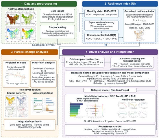
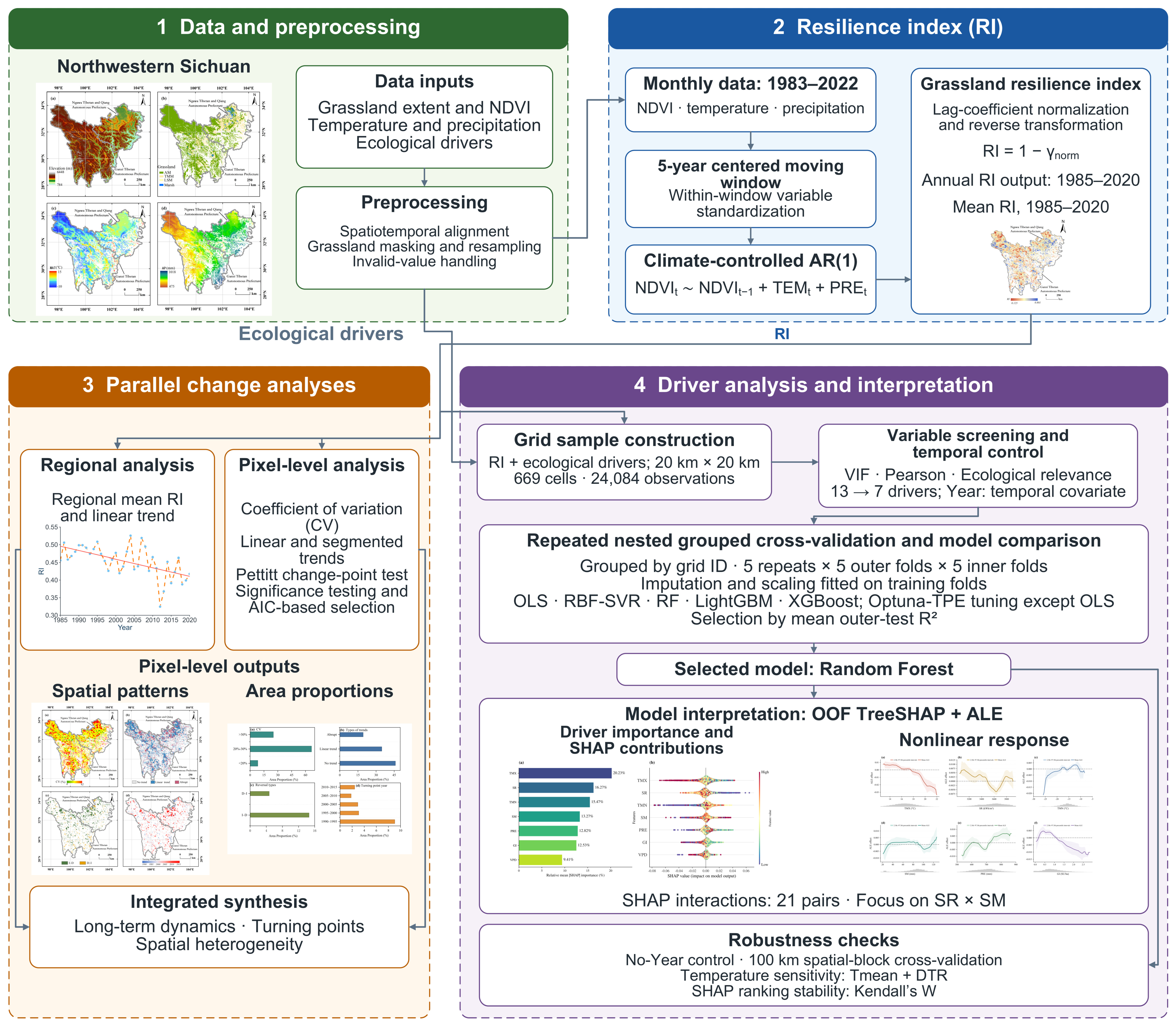
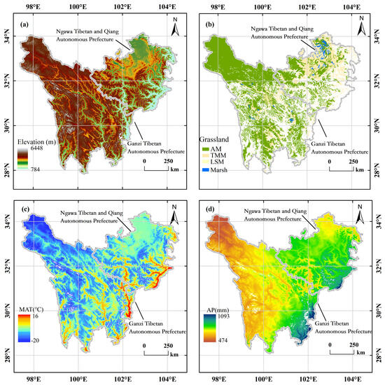
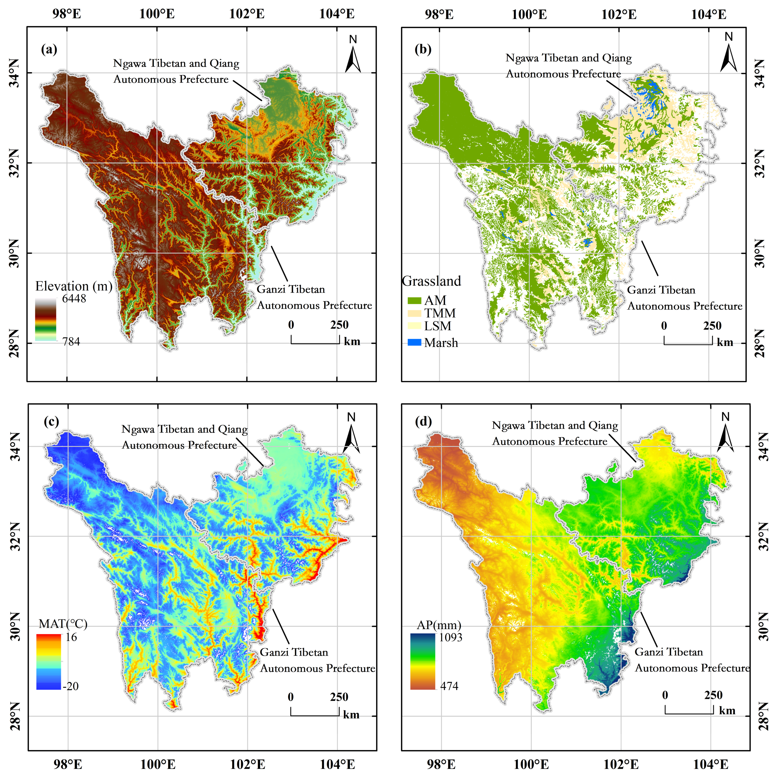
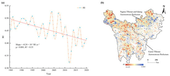
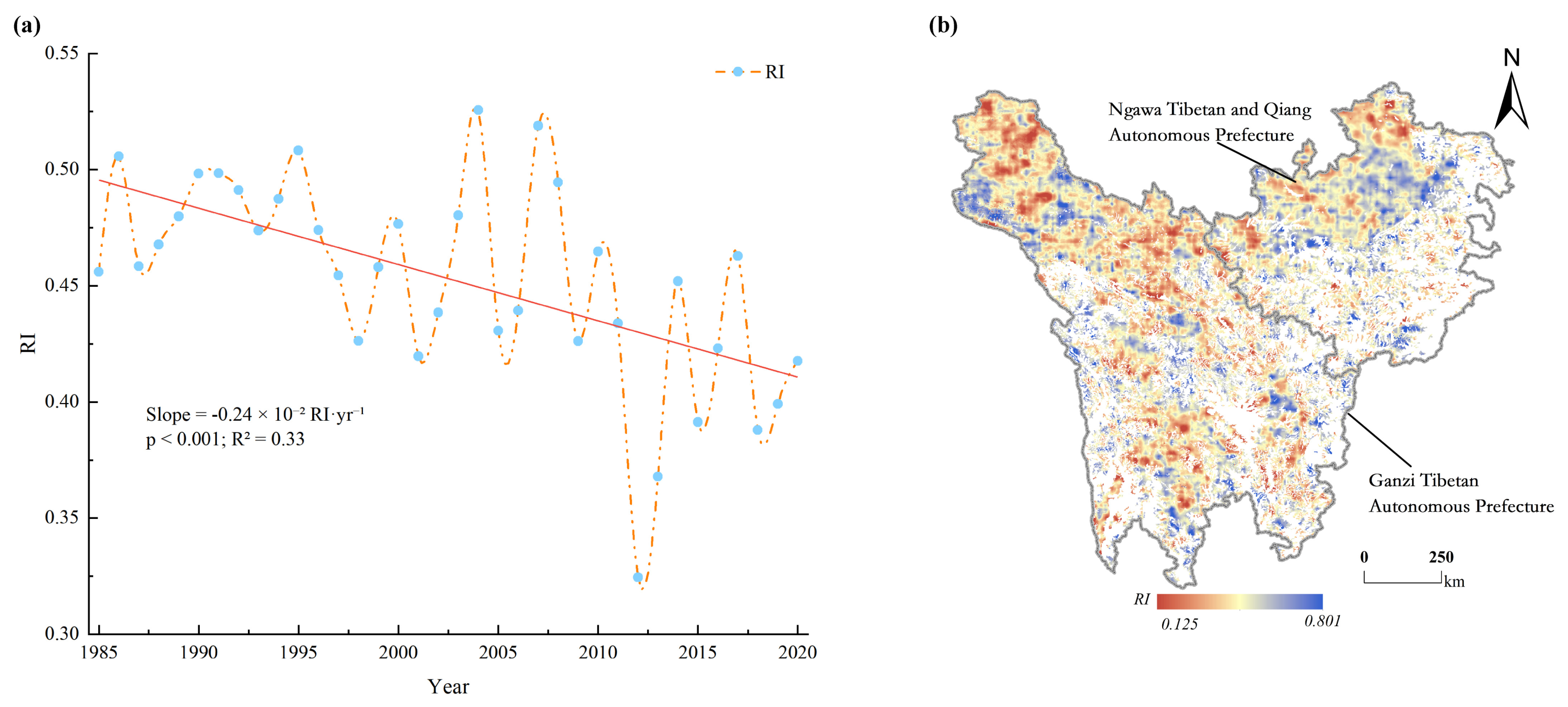
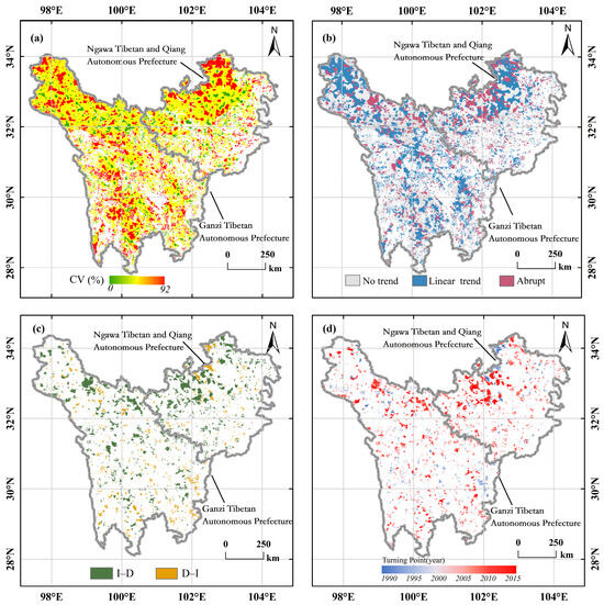
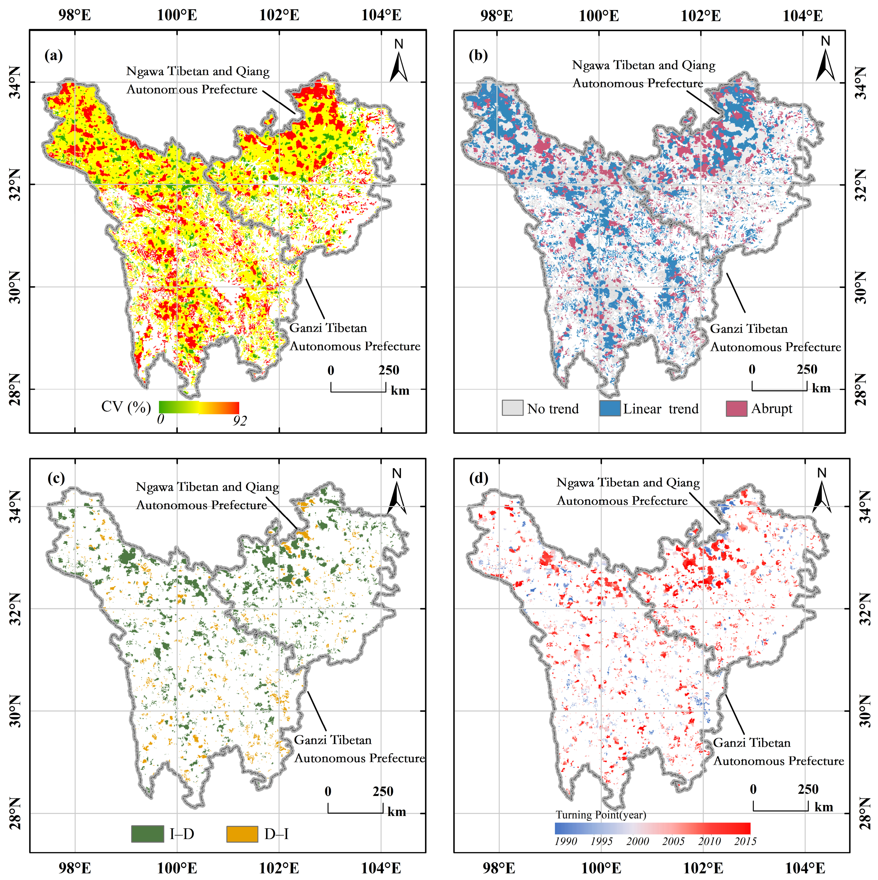
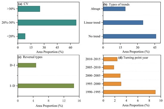
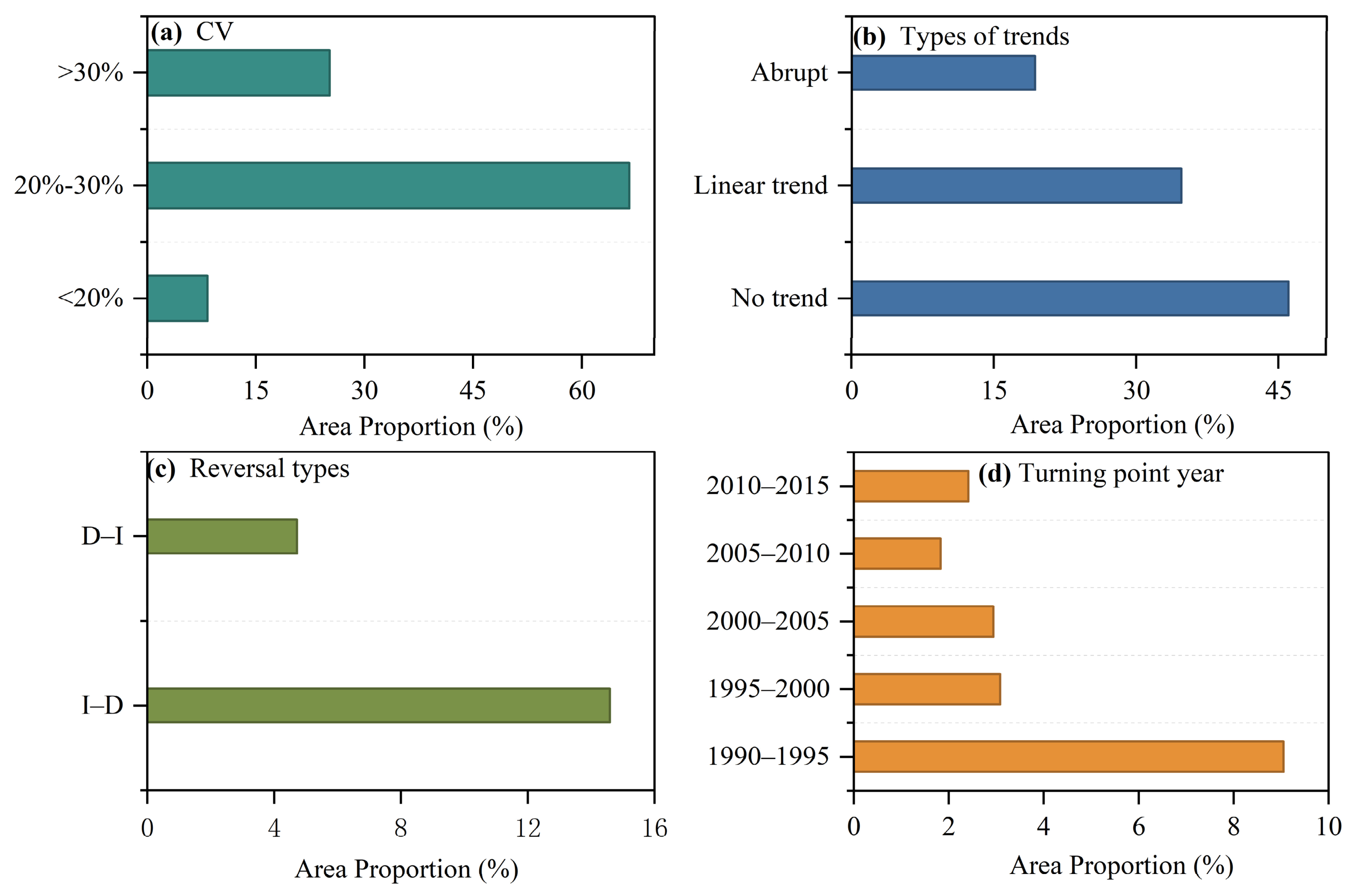
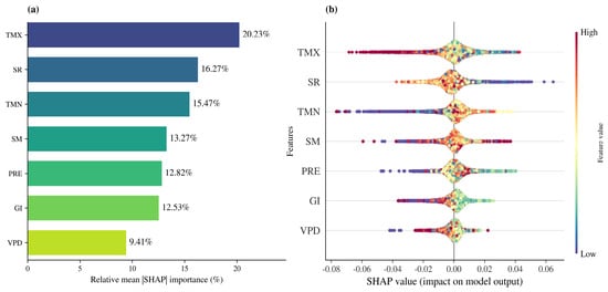
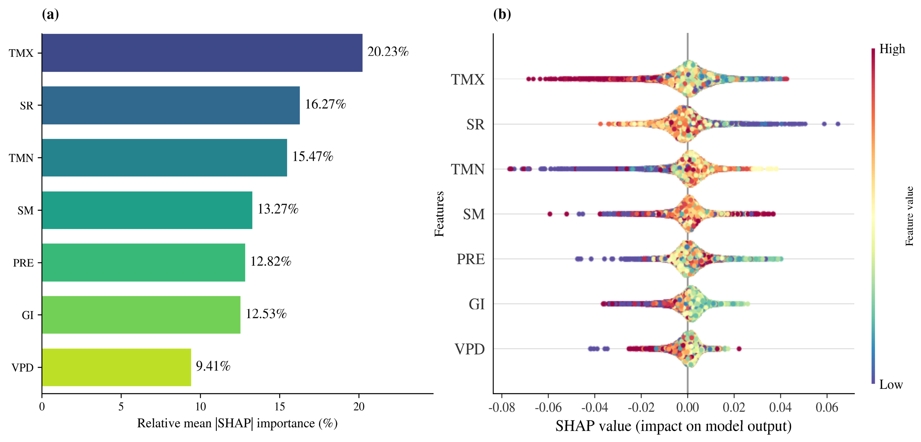
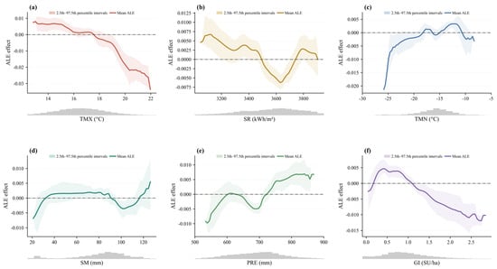
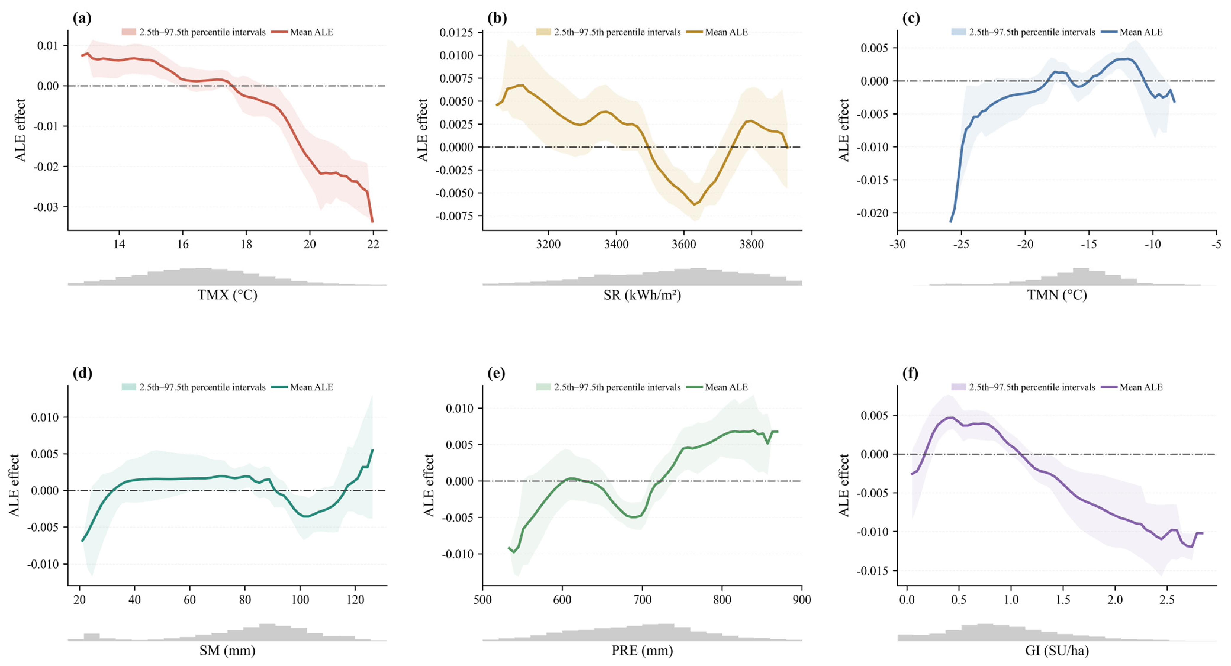

Disclaimer/Publisher’s Note: The statements, opinions and data contained in all publications are solely those of the individual author(s) and contributor(s) and not of MDPI and/or the editor(s). MDPI and/or the editor(s) disclaim responsibility for any injury to people or property resulting from any ideas, methods, instructions or products referred to in the content. |
© 2026 by the authors. Licensee MDPI, Basel, Switzerland. This article is an open access article distributed under the terms and conditions of the Creative Commons Attribution (CC BY) license.