


Abstract
Plant biologists routinely screen gene–metabolite correlations for regulatory hypotheses. Most such studies use ordered designs and carry two problems that are rarely addressed. Reported statistics often omit the sample basis, and two variables drifting with time correlate regardless of regulatory links. We re-analyzed public supplementary data of a published rubber tree (Hevea brasiliensis) genome study. Inverting one published r–p pair recovered a sample size of n = 9. Merging 70 of the 663 entries left 593 unique key. A null benchmark from 400,000 Monte Carlo trials put the expected p < 0.05 rate at 5.03%. The published ordered-design matrix returned 34.3% of its 16,560 pairs with p < 0.05, 6.8-fold above expectation, consistent with shared time trends. Our six-step protocol removed 96.56% of original calls among 26,520 gene–metabolite pairs: 179 of the 5197 original calls (3.44%) retained support, and 2.76% of the 26,520 pairs (731 pairs) passed the within-stage permutation screen, below the 4.61% null expectation. We provide a self-check, benchmarks and a minimal reporting standard; centering can remove genuine responses, so the protocol is a prioritization step rather than an exclusion criterion. For nuisance-trend designs, significant entries from an un-de-trended matrix should not be cited as regulatory evidence.
1. Introduction
Plant biologists routinely pair a metabolome with a transcriptome, then screen the gene–metabolite correlations for regulatory hypotheses [1,2]. For each pair, a Pearson correlation is computed across samples, and pairs that pass a p value or adjusted q value cutoff are advanced as candidate regulatory relationships [3,4,5,6,7,8]. Ordered designs dominate this literature, whether developmental stage series, drought and cold time courses, fruit ripening stages, or the successive tapping events in the example below. The samples sit in a fixed time order, and the metabolic reprogramming that tracks that order is usually what the investigator set out to capture. These designs differ in how time enters the biology. Developmental and ripening series are often the object of study, whereas in stress and tapping series the time-ordered treatment is frequently a nuisance factor; the protocol below is intended for the latter situation, while still reporting both versions of every result so that genuinely stage-associated responses remain visible.
Ordered designs bring two problems. b One is reporting. Plant omics papers often publish r and p values in long supplementary tables but omit the sample size n, the test used and the scope of the multiple-testing correction. Minimum reporting standards for metabolomics have existed for years [9], yet these details are still frequently missing. Without those details, a reader cannot check whether a reported p-value is consistent with its degrees of freedom. The other problem is spurious correlation, which the design itself creates. When samples are ordered in time, many genes and metabolites drift along monotonic or near-monotonic paths, and two of them can correlate at close to ±1 for no biological reason. Statisticians have known about this for over a century [10,11,12]. Routine plant omics integration still rarely measures it and almost never corrects it with an explicit protocol, so candidate lists driven by a shared time component keep showing up in the literature. Established alternatives do not close this gap at these sample sizes. Partial correlation with time as a covariate removes only the linear component of the trend [13], and time-course modeling frameworks [14,15] are designed for longer series with more time points; neither supplies an auditable, replicate-aware permutation test for three-stage, three-replicate designs.
To quantify the bias and to offer a remedy, we needed a public plant multi-omics dataset built on a typical ordered design. A telomere-to-telomere (T2T) genome study of rubber tree [16], hereafter the source study, supplied one. Its supplements carry quantitative values for 663 metabolite entries measured in nine latex samples drawn from three stages, the tapping stages T1 and T7 and the untapped control TN, each with three biological replicates. The same nine samples also produced latex transcriptome libraries, and the study releases a correlation matrix of 92 candidate transcription factors against 180 metabolites. The main text singles out one representative correlation, between mevalonic acid (MVA) and HbMVK1, at r = 0.921212834 and p = 0.000418. Its sampling structure is typical of plant omics integration studies: three ordered stages with three replicates each, the smallest design at which within-stage permutation remains possible, and paired metabolite and transcript measurements on the same nine latex samples. It is therefore a stringent test case rather than an unusually favorable one. The protocol acts on the ordered design structure rather than on any tissue- or species-specific biology, so the demonstration does not hinge on latex metabolism being typical of plant systems.
We use this dataset as a worked example, not as an object of study, and we ask one methodological question: how much of a published ordered-design correlation matrix survives once its sample basis is established and its shared time trend removed? We answer in four steps. First, we invert one published r-p pair to recover and confirm the sample basis of the correlation analysis. We then build a metabolite quality-control step on five-tuple deduplication of isomeric and synonym duplicates. Next, we derive the null benchmark for correlation testing at n = 9 by Monte Carlo simulation and measure how far the observed correlations depart from it. Last, we propose a six-step de-trending protocol, run it end to end on the gene side, and supply benchmark values and code that others can reuse.Every number we report can be recomputed from the public supplementary files of the source study [16], together with the analysis code and reference tables provided with this article (see the Data Availability Statement).. The new element is the integration rather than the individual statistics: an exact sample-basis check, domain-keyed metabolite deduplication, a Monte Carlo null, and within-stage permutation of a centered matrix are combined into one auditable workflow with paired before-and-after reporting. The 71 MADS-box members serve as the worked gene family because they are a clearly annotated regulatory family in this genome, not because of any special link to latex biology.
2. Results
2.1. Sample Basis: Confirmation and Uniqueness of n = 9
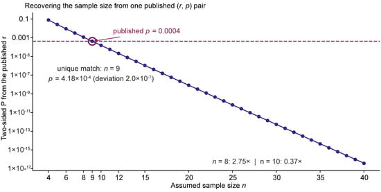
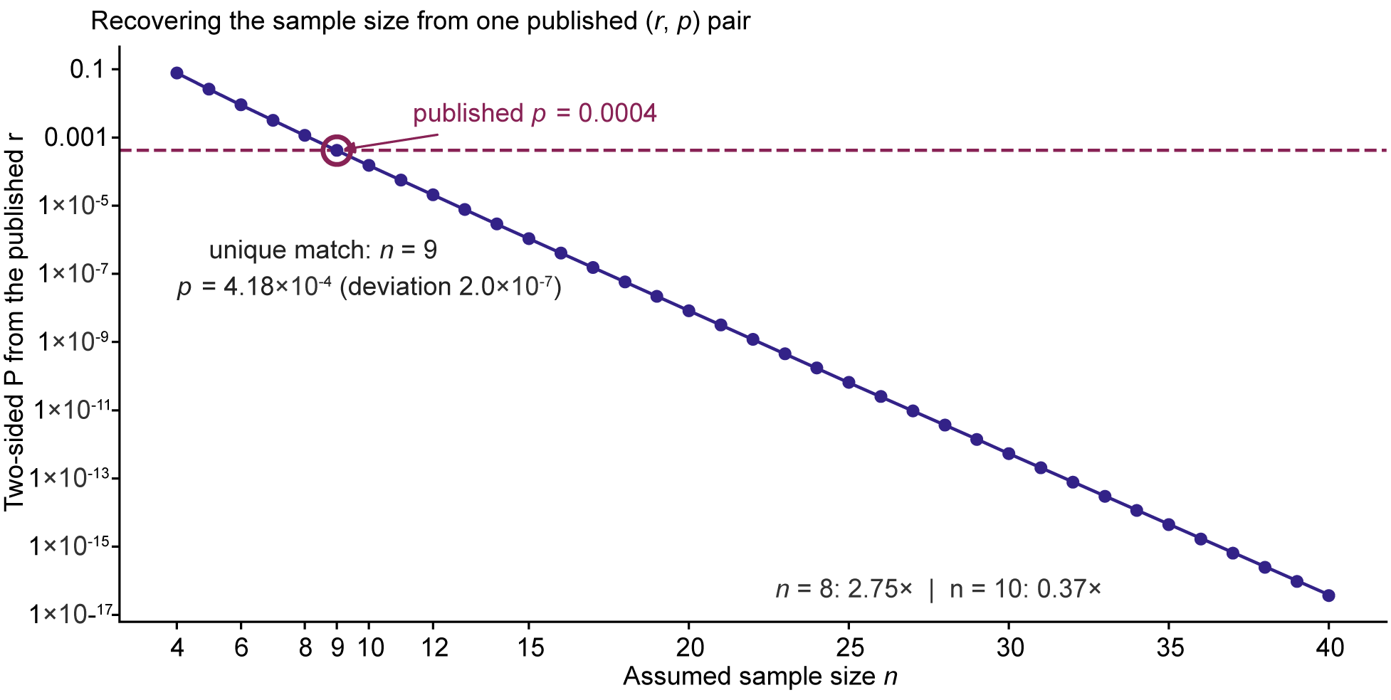
We inverted the MVA-HbMVK1 correlation reported in the source study (r = 0.921212834, p = 0.000418) and obtained t = 6.2646 with seven degrees of freedom, hence p = 0.00041820 at n = 9. That value lies 2.0 × 10⁻⁷ from the published one, a relative deviation of 0.05%. We then scanned the control range from n = 4 to n = 40 (Table 1; the full range is given in Table S1). Only n = 9 reproduces the published p (Figure 1): at n = 8, the computed p is 2.75 times the published value, and at n = 10, it is 0.37 times, both far outside any rounding tolerance. The correlation analysis of the source study therefore rests on nine samples, three tapping stages with three biological replicates each, and every recalculation below uses that basis. The same nine samples underlie the full correlation matrix in Supplementary Data 27of the source study [16].
Table 1.
Sample-size back-calculation from the published r-p pair (r = 0.921212834; two-sided t test; computed in this study).
Figure 1.
Back-calculation of the sample basis. Two-sided p computed from the published r = 0.921212834 over assumed sample sizes n = 4 to 40 (logarithmic vertical axis). The dashed line marks the published p = 0.000418, and the open circle marks the unique match at n = 9, where the recomputed p is 4.18 × 10⁻⁴ (deviation 2.0 × 10⁻⁷, or 0.05%). Ratios at n = 8 (2.75×) and n = 10 (0.37×) are annotated.
2.2. Five-Tuple Deduplication: 663 Entries to 593 Keys, with 12 Contradictory Groups
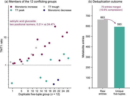
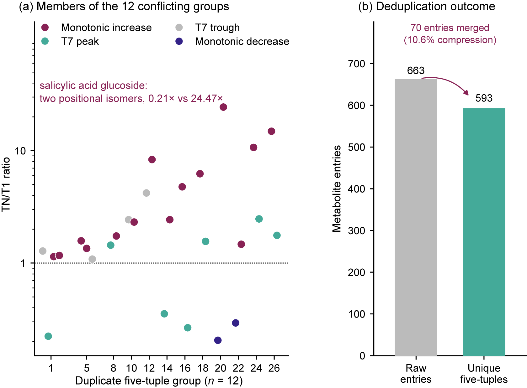
De-duplicating the 663 metabolite entries on a five-tuple key (molecular formula, molecular weight, precursor ion m/z, product ion m/z, ion mode) collapsed them to 593 unique keys and left 70 redundant entries, about 10.6% of the total (Figure 2). The merge also surfaced 12 groups whose members match on every parameter but move in opposite kinetic directions (Table 2 and Table S2). If left unmerged, entries like these reach a correlation matrix as near-identical rows, return near-identical r values, and let one biological signal be counted several times by any downstream test that works off member counts. The 12 groups are heterogeneous in kind. Group 20 separates two positional isomers of salicylic acid glucoside, the 2-O-glucoside and the 1-O-acyl glucoside, whose TN/T1 ratios differ about 100-fold (0.21 and 24.47; Figure 2). Group 22 is a nomenclatural duplicate rather than an isomeric collision: one entry carries the trivial name inosine and the other its systematic name, yet the source table files them under different chemical classes with opposite trajectories (TN/T1 0.29 and 1.47). The remaining groups are isomer merges (positional or structural), which the five-tuple key cannot resolve; Table 2 classifies each group, and the merged set is reported as candidate duplicates rather than confirmed chemical identities.
Figure 2.
Five-tuple deduplication of 663 metabolite entries. (a) TN/T1 ratios of the 27 entries that form the 12 directionally contradictory five-tuple groups, plotted on a logarithmic axis by group; colors denote trajectory class (monotonic increase, monotonic decrease, T7 peak and T7 trough). The salicylic acid glucoside group, in which two positional isomers differ by roughly 100-fold, is annotated. dotted line, TN/T1 = 1. (b) Entry counts before (663) and after (593) merging; 70 entries were merged, a compression of 10.6%.
Table 2.
The 12 five-tuple groups whose members share every key field but disagree in kinetic direction.
2.3. Null Benchmark: The Background Rate of Significance at n = 9
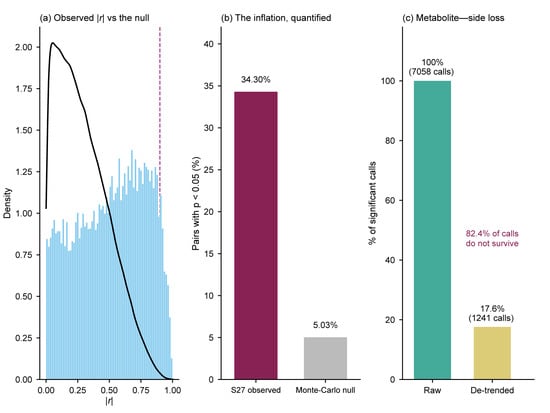
For pure-noise series of length 9, the 400,000 Monte Carlo trials returned p < 0.05 in 5.03% of cases and |r| > 0.9 in 0.098%. Both are close to the nominal 5% and 0.1%, a good sign that the simulation is working as intended. The source correlation matrix (92 genes × 180 metabolites, 16,560 pairs; Pearson r at n = 9, Section 4.1) is another matter. There 34.3% of pairs had p < 0.05, 6.8 times the null expectation, and |r| > 0.9 in 5.7% of pairs, a 58-fold excess (Figure 3a,b). In this ordered design, the excess of significant pairs is consistent with a shared time trend, although the generic null cannot exclude contributions from other structure in the biological data; no regulatory relationship is required to explain it.
Figure 3.
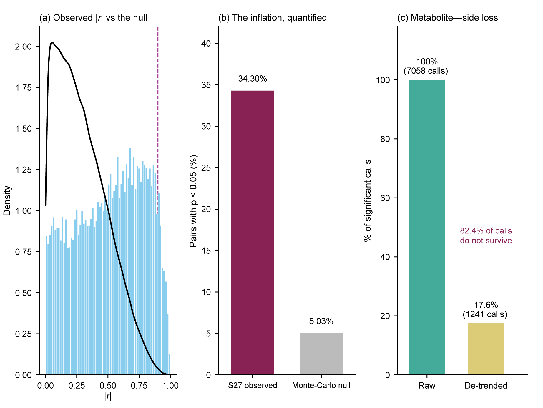
Observed correlation strength against the null, and metabolite-side de-trending. (a) Distribution of |r| for the 16,560 entries of the source correlation matrix (92 genes × 180 metabolites), with the n = 9 Monte Carlo null overlaid; the dashed line marks |r| = 0.9. (b) Fraction of pairs with p < 0.05 in the observed matrix (34.3%) and under the null (5.03%). (c) Metabolite-side calls before and after de-trending, expressed as a percentage of the calls identified before de-trending (19,966 draws tested; 7058 calls before de-trending, of which 1241, or 17.6%, survived).
2.4. Metabolite-Side De-Trending
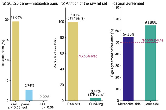
We ran the same check on the metabolite side to confirm that the inflation comes from the design rather than from the gene–metabolite matrix. We drew 20,000 metabolite pairs at random with replacement, dropped 34 self-pairs and kept 19,966. We computed correlations on the raw values and again after within-stage centering, then tested both sets with a two-sided t test (df = 7). Before centering, 35.4% of the draws (7058) had p < 0.05. After centering, 17.6% of those calls (1241) survived, so 82.4% were lost (Figure 3c). Applying the degrees-of-freedom correction of the full protocol (df = 5 after centering) strengthens the effect: only 808 calls (11.4%) survived; The main comparison uses a two-sided t test with df = 7 on both sides. On the 19,122 distinct pairs the corresponding figures are 6752 raw calls and 1181 survivors (82.5% lost), showing that duplicate sampling does not drive the result. The sign of r agreed before and after centering for 54.8% of the 19,966 draws, close to the 50% expected when the between-stage trend is removed and no within-stage association exists. The main comparison applies a single t test with df = 7 on both sides so that centering is the only change; the df-corrected comparison is reported alongside (11.4% survival, 88.6% lost). Figure 3c shows the df = 7 comparison.
2.5. Full Gene-Side Execution: 40 MADS-Box Members Against 663 Metabolites
We applied the six steps to the 40 MADS-box members that retained within-group variance in latex, against 663 metabolite entries, which gave 26,520 pairs. This matrix differs from the 92-gene S27 matrix analyzed in Section 2.3: the S27 matrix quantifies the inflation in the published source analysis, whereas the 40-member matrix is our own from-scratch demonstration, so the percentages describe different pair sets and are not a before-and-after comparison of one matrix. The other 31 members had no residual variance after centering, so their 20,553 pairs cannot be tested at all; they are not failed tests. All 31 had TPM = 0 in all nine latex samples (no detectable expression, hence no residual variance). Within the 40 testable members, 23 had low but nonzero expression (mean TPM ≤ 1) and measurable variance. Exclusion therefore restricts the analysis to members with measurable, variable latex expression, which is the relevant population for a correlation screen. Before de-trending, 19.60% of the 26,520 pairs reached parametric p < 0.05. After within-stage centering, 2.76% passed the within-stage permutation test (Figure 4a). Under the restricted permutation null, the expected pass rate is 4.61%, because (b + 1)/217 ≤ 0.05 corresponds to b ≤ 9, so the rejection region has probability 10/217 = 4.61%. The observed 2.76% (731 of 26,520; 95% CI 2.56–2.96%) lies below this expectation, the conservative direction produced by centering. The parametric reference at df = 5 gives 6.21% (|r| > 0.7545), above the nominal 5% level, so the parametric test is mildly liberal on centered residuals and inference rests on the permutation test; 96.56% of the 5197 original calls lost significance, which left 179 survivors. The remaining 552 of the 731 passing pairs had not been significant before de-trending, which follows because centering shifts both |r| and its sign. No pair survived dual Benjamini–Hochberg correction (Figure 4a). Among the 5197 original calls, the sign of r was unchanged before and after de-trending for 64.86% of pairs (Figure 4c).
Figure 4.
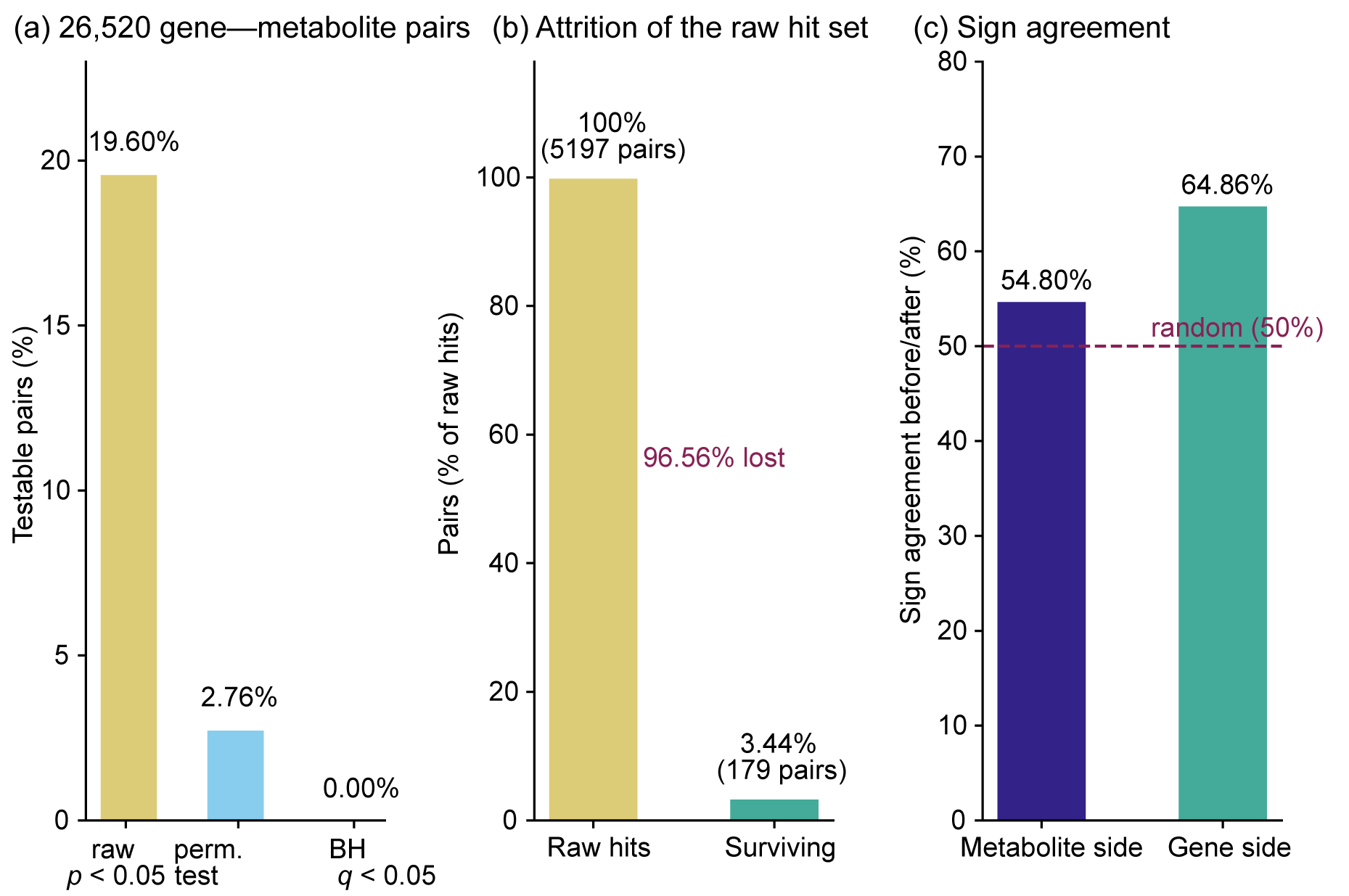
Gene-side execution of the six-step protocol on 26,520 gene–metabolite pairs. (a) Three different statistical procedures are shown separately: the parametric t test before de-trending (19.60%), the within-stage permutation test after de-trending (2.76%) and dual Benjamini–Hochberg correction (0.00%). (b) Attrition of the 5197 original calls: 179 pairs (3.44%) remain significant, so 96.56% are lost. (c) Agreement in the sign of r before and after de-trending, with the two sides computed on different denominators: all 19,966 metabolite draws (54.8%) and the 5197 originally significant gene–metabolite pairs (64.86%). The dashed line marks the 50% expected for random sign.
2.6. Sensitivity: The Resolution Limit of 216 Permutations
Within-stage permutation of three replicates across three stages allows (3!)3 = 216 arrangements, so no pair can have a permutation p below 1/217 ≈ 0.0046. No single pair can therefore be shown to be significant below that level, and dual BH correction across 26,520 pairs would need a p near 1.9 × 10⁻⁶ for rank one, which this permutation scheme cannot reach. The zero count in Figure 4 reflects that resolution limit; it does not mean that no association exists. Our inference rests instead on the set-level statistic, the fraction of pairs that pass. That statistic still carries information because 2.76% shows no excess over the within-stage null (expected 4.61%). If single-pair resolution is needed, add a parametric null or a bootstrap with more resamples. For example, four replicates per stage expand the within-stage permutation space from (3!)3 = 216 to (4!)3 = 13,824, which permits much finer empirical p-value resolution; empirical-Bayes shrinkage is an alternative when the design cannot be enlarged.
2.7. Benchmark Summary
Table 3 gathers the numbers readers can reuse directly: the null expectations at n = 9, the two excess ratios, the loss and sign-concordance figures for both sides of the analysis, and the resolution limit of the permutation scheme. Together, they set expectations for a matrix built on three time points with three replicates each.
Table 3.
Quantitative benchmarks for correlation analysis under an ordered time-point design (n = 9, this study).
3. Discussion
3.1. A Thirty-Second Check on the Sample Size
Take any r-p pair from the supplement of a plant omics paper, provided the study used the standard t test. Substitute the pair into t = r√[(n − 2)/(1 − r2)] and p = 2Pr(Tn−2 > |t|), then scan n from 4 to 40 for the value that reproduces the published p (Table S1). If exactly one value matches within rounding, the sample size is confirmed, and you can compute the study’s statistical power. If none does, r and p are inconsistent, most likely because a different test was used, or adjusted p-values were reported as raw ones. If several values match, as happens when r is near zero, the pair says nothing about n. The check is not restricted to metabolomes or to rubber tree; any omics dataset will do.
3.2. Deciding Whether a Matrix Is Contaminated
Our simulation puts the n = 9 expectation at 5.03% of pairs for p < 0.05 and 0.098% for |r| > 0.9. Count the same two fractions in your own matrix and compare. Close agreement argues against serious contamination. An excess of several-fold, as here (6.8-fold), makes time-trend confounding the first suspect. The same recipe gives benchmarks for other sample sizes: draw two independent standard normal series of length n and repeat 105 to 106 times.
3.3. Minimal Execution Set and a Reporting Standard
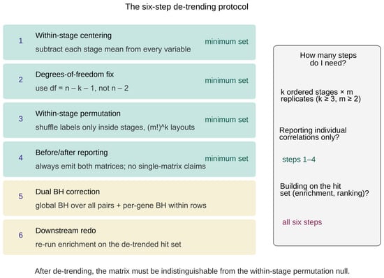
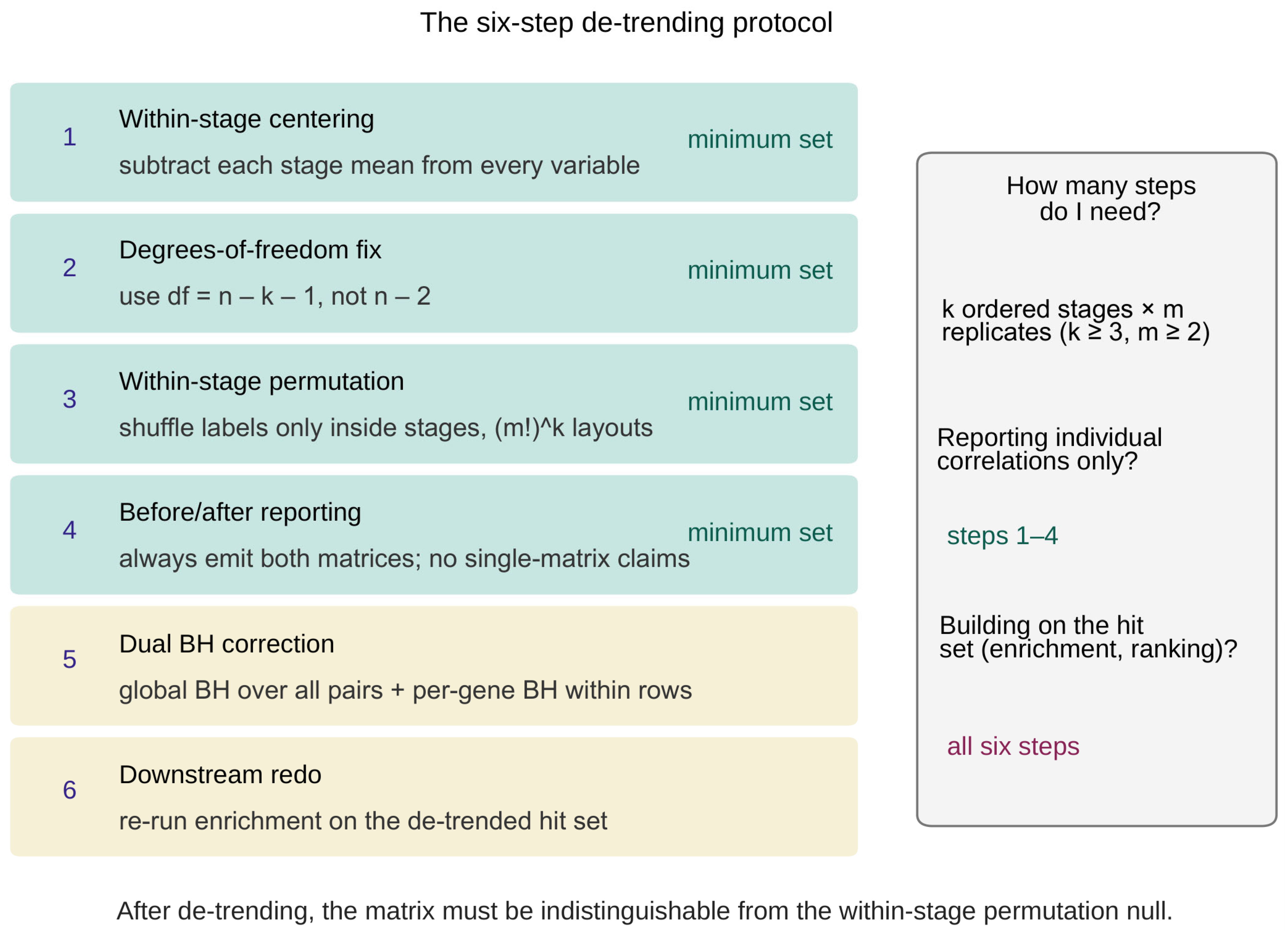
For a design of k ordered time points with m replicates each (k ≥ 3, m ≥ 2), four steps are the minimum. First, subtract the stage mean of every variable within every stage. Second, test correlations with = n − k − 1 instead of n − 2; the permutation test in step 3 does not use this value. Third, assess significance by permuting labels only inside stage blocks, (m!)ᵏ arrangements in total, so that temporal order survives. Fourth, report raw and de-trended values side by side. Two more steps matter when the significant set feeds enrichment of categories or pathways, or a candidate ranking. Apply dual BH correction globally and within each gene row, then re-run the downstream analysis on the de-trended set (Figure 5). Deposit both matrices, raw and de-trended, in the supplement or a public repository such as MetaboLights [17]; record the sample size, the test, degrees of freedom and correction scope in the table or its legend. A series with m = 1 has no within-stage variance and falls outside the protocol [18].
Figure 5.
The six-step de-trending protocol. Steps 1 to 4 (within-stage centering, degrees-of-freedom correction, within-stage permutation and paired reporting) form the minimal execution set. Steps 5 and 6 (dual Benjamini–Hochberg correction and re-analysis of downstream results) are required when the significant set feeds category enrichment, pathway enrichment or candidate ranking.
3.4. Alternatives, Boundaries and Limitations
Each alternative has a cost. Model-based de-trending with splines, local regression or mixed models [14,15,19,20,21] needs more than three time points. Surrogate-variable and factor-based normalization [20,21] target latent technical structure, which is not the same problem as a trend built into the design. Non-regulatory sources of correlation in metabolomic data are well documented [13,22,23,24]. The obvious fix for a trend is partial correlation with time as a covariate [13]. At n = 9 it pays the same degrees-of-freedom penalty as centering, but it strips out only the linear part of the trend; within-stage centering handles any between-stage mean structure, linear or not. The four-step minimum therefore fits a narrow but common niche: few time points, several replicates per point, and a trend that is a nuisance rather than the signal. A partialling out stage as a categorical factor is algebraically equivalent to within-stage centering and carries the same loss of degrees of freedom; the contribution here is not the centering itself but the exact sample-basis check, the permutation-based inference and the paired reporting that make the correction auditable at n = 9.
The protocol has limits too. With m = 1, centering leaves nothing, so differencing or a model-based trend is needed instead [14,15,19,20,21]. As k grows, the shared trend contributes less to the correlation, but the permutation space grows as (m!)k, so a bootstrap or a parametric null becomes the practical choice. Centering also removes any true monotonic dose-response that runs with the trend, which is why paired reporting is not optional. The benchmark itself is one limit: it comes from a single dataset, and the 6.8-fold and 58-fold ratios reflect that dataset’s particular trend structure, so other studies should run their own simulations rather than cite these numbers. Resolution is another: with only 216 permutations, single-pair resolution stops at 0.0046, leaving dual BH correction uninformative across 26,520 pairs. The gene-level analysis lost 31 of the 71 MADS-box members to zero residual variance, so its conclusions cover only the 40 testable members. Finally, the five-tuple key inherits the annotation quality of the source table because we did not re-examine the underlying peak areas. De-trending should therefore be read as a hypothesis-prioritization filter, not an exclusion criterion: candidates that survive it warrant follow-up by targeted functional assays, such as transient overexpression, CRISPR knockout or metabolic perturbation, rather than being accepted on statistical grounds alone. One further assumption is not testable from the source files: the coefficients in Supplementary Data 27 are taken to be Pearson r because Supplementary Data 19 names Pearson correlation and the source Methods cite corrplot, whose default is Pearson’s r. corrplot is a visualization package, so this remains an inference; if a rank-based coefficient had been used, individual |r| values would differ, but the excess over the null and the effect of centering would remain. With three replicates per stage the design fixes the resolution of the permutation test rather than the precision of the stage means; our inference is therefore set-level (the share of pairs passing the screen), and single-pair calls at this design are reported only as descriptive. Beyond this dataset, the correction uses only stage labels and replicate membership, so it transfers directly to any ordered design (developmental series, dose gradients or stress time courses) in any species or platform, and larger replicate numbers can only improve permutation resolution and power.
3.5. What This Means for Published Correlation Matrices
A 6.8-fold excess of p < 0.05 calls and a 58-fold excess of |r| > 0.9 are large enough to change how one reads the literature. In matrices built on three time points with three replicates per point, as here, a shared time trend can account for a substantial share of the reported associations. None of these limitations undermines relationships that independent experiments have validated.. The JA-MYC2-HbMVK1 axis in the source study [16] is supported by dual-luciferase and yeast one-hybrid assays, independent of any matrix value; the same applies to the broader MYC2 literature on jasmonate signaling [25]. These caveats do, however, affect candidate lists derived solely from matrix significance. Such lists should be treated strictly as hypothesis-generating until the underlying trend is removed, unless the temporal variation is itself the biological response of interest; in that case within-stage centering is the wrong tool because it removes the very signal the experiment was designed to detect.
4. Materials and Methods
4.1. Data Sources
All inputs are drawn from public supplementary files of the source study [16]. Supplementary Data 18 contains the quantitative matrix of 663 metabolites across nine latex samples from stages T1, T7 and TN, while Supplementary Data 13 provides the sample-to-stage mapping. Supplementary Data 21 lists 91 candidate transcription factors. Supplementary Data 27 contains a correlation matrix for 92 genes against 180 metabolites; notably, the additional gene HbAchr1M0001995 is not among the 91 candidates. Supplementary Data 19 offers a similar matrix, described as a Pearson correlation analysis between rubber biosynthesis genes and differentially accumulated metabolites. However, Supplementary Data 27 reports coefficients only, without sample sizes or statistical tests, and the parenthetical note in its title refers to the GO enrichment used for gene selection rather than to the correlation test itself. The test itself is the standard Pearson t test: Supplementary Data 19 states Pearson correlation explicitly, and the source Methods name corrplot v0.92, whose default is Pearson’s r. The sample basis is n = 9, the nine matched latex samples that carry both omics layers, the same value we recovered uniquely from the MVA-HbMVK1 pair in Section 2.1. The nine latex transcriptome libraries (CRR998972 to CRR998980) are archived at the National Genomics Data Center under PRJCA022207. We aligned reads with STAR 2.7.11b (Cold Spring Harbor Laboratory, Cold Spring Harbor, NY, USA) [26] to the chromosome-level GT1 reference genome [27] (GCA_010458925.1), counted them with--quantMode GeneCounts, and converted the counts to transcripts per million (TPM). No expression threshold was applied to the MADS-box expression values; exclusion from the correlation analysis was based solely on residual variance after within-stage centering (Section 2.5). The three stages used here are the tapping stages T1 and T7 and the untapped control TN, each with three biological replicates. We identified the 71 MADS-box family members with pyhmmer 0.12.3 hmmsearch [28] against PF00319.24 and PF01486.23, with inclusion at the Pfam gathering threshold [29]: candidates were retained only when the PF00319 alignment itself met the threshold, truncated domains that failed it were excluded, and proteins with multiple domain matches were assigned by the highest-scoring match. PF01486 (K-box) was used only for type II classification, not as an inclusion requirement; locus identifiers, closest homologues, clades and unified names are listed in Table S4. The MADS-box list was derived from the proteome independently of expression: 31 of the 71 members had no detectable latex expression (TPM = 0 in all nine samples) and therefore no residual variance after centering, which left 40 testable members; 23 of the 40 had low but nonzero expression (mean TPM ≤ 1) and were retained. TPM values were computed from effective gene lengths taken from the GT1 annotation GTF (GCA_010458925.1, genomic.gff) and scaled to library size, so that each library sums to one million. Because corrplot is a visualization package, this assignment remains an inference; we therefore treat the Pearson basis as a documented assumption and note it as a limitation in Section 3.4.
4.2. Back-Calculation of the Sample Basis
We inverted the Pearson t test for the published r-p pair: t = r√[(n − 2)/(1 − r2)], with two-sided p = 2Pr(Tn−2 > |t|). We evaluated candidate values of n one at a time and accepted the value whose relative deviation fell below 1%. A control table over n = 4 to 40 tested uniqueness. All computation used the Python 3.12 (Python Software Foundation, Wilmington, DE, USA) standard library, with the t survival function evaluated from a continued-fraction expansion of the incomplete beta function, and the published p served as an inline check.
4.3. Five-Tuple Deduplication
We merged the entries of Supplementary Data 18 on a key of five fields: molecular formula, molecular weight, precursor ion m/z, product ion m/z and ion mode. We collapsed duplicate identifications of the same compound at this level, including isomeric entries flagged 2n and synonyms [30,31,32]. After merging, we checked each group for directional consistency across the three stages and listed the groups that disagreed rather than averaging them. Trajectory classes were assigned from the stage means: monotonic increase (T1 < T7 < TN), monotonic decrease (T1 > T7 > TN), T7 peak (T7 above both T1 and TN) and T7 trough (T7 below both). A group was counted as contradictory if it held at least one monotonic increase alongside members of any other class. The three numeric fields of the key were rounded to three decimals by design, not for appearance: on the reference data, this gave 593 unique keys, against 594 at four decimals and 595 unrounded. An explicit rounding function enforces the convention, which stops floating-point representation from splitting keys. The key establishes shared annotation parameters, not chemical identity: structural or positional isomers can coincide on all five fields, so merged groups are reported as candidate duplicates rather than confirmed synonyms. Retention time and MS/MS spectral similarity were not available in the source table and would be required to confirm chemical identity. Three decimals (1 mDa) is far coarser than the mass accuracy of the high-resolution platform (parts per million), so true replicate measurements of one compound fall on the same key, while entries differing by ≥2 mDa remain separate; the sensitivity is small in any case because four decimals yield 594 keys and unrounded values 595.
4.4. Monte Carlo Null
We benchmarked correlation significance on pure noise at n = 9 with 400,000 Monte Carlo trials (random seed 20261005). Each trial drew two independent standard normal series of length 9 and recorded the Pearson r and its p-value. We then compared the empirical fractions of p < 0.05 and of |r| beyond the chosen thresholds against the values measured across the matrix. Block-mean stability checked convergence (Table S3): across ten blocks of 40,000 trials, the block means of the p < 0.05 fraction averaged 5.031% with a standard deviation of 0.096 percentage points (range 4.877 to 5.190); |r| > 0.667 gave 5.000% ± 0.096 and |r| > 0.8 gave 0.969% ± 0.043. The null is deliberately generic: it reproduces the nominal significance rate but not the stage-dependent distributions, within-stage variability or dependence structure of real omics data. We therefore use it only to quantify the excess over random expectation. Design-matched inference comes from the within-stage permutation (Section 4.5), which is nonparametric: randomizing only the pairing of replicates within each stage preserves the stage-dependent distributions and the within-stage variability of the actual measurements exactly, by construction. The attribution of the observed excess to between-stage mean structure, rather than to within-stage dependence, rests on the before-and-after de-trending contrast (Section 2.4 and Section 2.5).
4.5. The Six-Step De-Trending Protocol
What follows assumes three ordered stages with three replicates each, though nothing in it depends on those numbers: with k stages and m replicates, the steps are the same.
1. Within-stage centering. Subtract the stage mean of each variable. What is left is within-group variation only.
2. Degrees-of-freedom correction. Centering uses one degree of freedom per stage and the correlation one more, so a parametric test on the centered residuals has df = n − k − 1 = 9 − 3 − 1 = 5, not n − 2 = 7.
3. Within-stage permutation. Shuffle the sample labels inside stage blocks [33,34], never across them. That gives 3! = 6 arrangements per block, 63 = 216 in total, and keeps the time order intact. Permutation P-values use the add-one convention (b + 1)/(216 + 1), which includes the observed arrangement, so the smallest attainable p is 1/217 rather than 1/216; the test is therefore marginally conservative (1/217 = 0.00461 versus 1/216 = 0.00463), and no conclusion depends on the choice.
4. Paired reporting. Report the pre- and post-de-trending values together. One without the other tells the reader little.
5. Dual Benjamini–Hochberg correction. Run BH correction [35,36] on all pairs globally and again within each gene row, then report both adjusted columns side by side, each labeled with its testing family. If you prefer a q-value or a dependency-aware estimate, those are available [37,38,39]. The global correction controls the false discovery rate across the entire 26,520-pair family, whereas the per-gene correction controls it within each gene’s 663 tests, a much smaller family; the two therefore answer different questions, are not equivalent levels of control, and each guarantee holds only within its own family. The two levels serve different downstream uses. The global level backs matrix-wide claims and is the conservative default for any statement about the dataset as a whole; the per-gene level backs gene-centric shortlists because a gene whose correlations are genuinely concentrated can lose every pair under the global family even though several pairs stand out within its own row. Reporting only the per-gene level would overstate matrix-wide evidence since each row carries its own false-discovery budget; reporting only the global level would discard signals concentrated in single genes. Reporting both, labeled by family, lets a reader match the correction to the claim being made, and neither column is used to re-select from the other. Bonferroni correction controls the family-wise error rate and is unnecessarily conservative for 26,520 correlated tests, whereas BH controls the false discovery rate, which matches the exploratory purpose of a correlation screen.
6. Downstream re-analysis. Anything that takes the hit set as input, enrichment tests for instance, must be re-run on the de-trended set. Earlier conclusions do not carry over.
Steps 1–4 are the minimum; they still apply when only one coefficient is reported. Steps 5 and 6 become mandatory once the hit set feeds category enrichment, pathway enrichment or candidate ranking.
For the metabolite-side check, we drew 20,000 entry pairs at random with replacement from Supplementary Data 18 (seed 20261005). Dropping 34 self-pairs left 19,966 draws, which cover 19,122 distinct pairs. Raw and centered correlations both went through a two-sided t test. The main comparison used df = 7 on both sides to isolate the effect of centering alone; a corrected comparison with df = 5 after centering is also reported. In addition, results were recomputed on the 19,122 distinct pairs as a sensitivity analysis for duplicate sampling.
4.6. Software and Reproducibility
The whole protocol is written in plain Python 3.12 with the standard library only; there are no third-party dependencies, so the code can be audited line by line and run without a general-purpose pipeline platform [40]. p-values for the t distribution come from a continued-fraction evaluation of the incomplete beta function, with the random seed fixed at 20261005. The package comprises four files: detrend_protocol.py, which provides four subcommands (backcalc, dedup, null, and selfcheck); validate.py, which performs 24 automated checks and passes all on the reference table; test_protocol_synthetic.py, which executes unit tests on synthetic data; and S18_reference.tsv, the exported reference table consumed by validate.py. The code is archived at Zenodo under an MIT license (DOI: 10.5281/zenodo.24157102). The df convention is n − k − 1 throughout the gene-side protocol; the metabolite-side demonstration compares df = 7 on both sides (Section 2.4)..
5. Conclusions
In plant multi-omics studies based on ordered time points, gene–metabolite correlation matrices exhibit two correctable defects: a missing sample basis and time-trend confounding. A published r–p pair can address the former; a null benchmark quantifies the latter; and the protocol presented here reduces it substantially in the three-stage, three-replicate setting demonstrated here. The first four steps form the minimum requirement; effectiveness in other designs remains to be validated. Applied to public rubber tree data, de-trending reduced the gene-side call rate from 19.60% to 2.76%. This rate shows no excess over the within-stage permutation null (expected 4.61%), indicating that residual calls cannot be distinguished from within-stage noise at the resolution afforded by 216 permutations, which does not by itself prove the absence of genuine gene–metabolite relationships.
Practitioners are advised to take three actions. First, verify the sample basis of any matrix using the self-check described in Section 3.1. Second, assess whether a matrix is contaminated against the benchmark in Section 3.2. Third, report raw and de-trended results side by side, as outlined in Section 3.3. For designs in which the time trend is a nuisance rather than the object of study, a matrix that has not been de-trended generates hypotheses rather than regulatory evidence.
Supplementary Materials
The following supporting information can be downloaded at: https://www.mdpi.com/article/doi/s1.
Author Contributions
Conceptualization, B.G.; methodology, B.G.; software, B.G. and Y.N.; validation, B.G. and Y.L.; formal analysis, B.G. and Y.N.; investigation, B.G.; data curation, B.G., Y.L. and J.A.; writing of the original draft, B.G.; writing of the review and editing, B.G., C.M. and J.L.; visualization, B.G.; supervision, C.M. and J.L.; project administration, J.L.; funding acquisition, J.L. All authors have read and agreed to the published version of the manuscript.
Funding
This research was funded by the Yunnan Technology Innovation Center of Natural Rubber (202605AK340010);Yunnan Provincial Basic Research Program (202401AS070083, 202601AS070002 and 202501CF070188);Yunnan Provincial Major Science and Technology Special Plan Projects (202602AE090106), Yunnan Academician & Expert Workstation Project (202605AF350029), the Yunnan Key Laboratory of Sustainable Utilization Research on Rubber Tree (202605AV340001), the Start-up Grant from Yunnan Institute of Tropical Crops (YITC2025-2) and the Yunnan Special Fund for Scientific and Technological Innovation of Tropical Crops (RF2026-2).
Institutional Review Board Statement
Not applicable.
Informed Consent Statement
Not applicable.
Data Availability Statement
All input data are the public supplementary files of the source study [16] (Section 4.1). The analysis code, the reference table and the benchmark outputs are openly available at Zenodo [41].
Acknowledgments
We thank Yuanyuan Zhang and Fei Li for responding to our inquiries about the sampling design and metadata of the public datasets used in this study. During the preparation of this work, the authors used DeepSeek (v 4.1)for language polishing and format checking only. The authors reviewed and edited all content and take full responsibility for the content of the publication. During the preparation of this work, the authors used DeepSeek for language polishing and format checking only. The authors reviewed and edited all content after using this tool and take full responsibility for the content of the publication.
Conflicts of Interest
The authors declare no conflicts of interest. The funders had no role in the design of the study, in the collection, analyses or interpretation of data, in the writing of the manuscript, or in the decision to publish the results.
References
- Fiehn, O. Metabolomics: The link between genotypes and phenotypes. Plant Mol. Biol. 2002, 48, 155–171. [Google Scholar] [CrossRef] [Scilit]
- Pinu, F.R.; Beale, D.J.; Paten, A.M.; Kouremenos, K.; Swarup, S.; Schirra, H.J.; Wishart, D. Systems biology and multi-omics integration: Viewpoints from the metabolomics research community. Metabolites 2019, 9, 76. [Google Scholar] [CrossRef] [Scilit] [PubMed]
- Urbanczyk-Wochniak, E.; Luedemann, A.; Kopka, J.; Selbig, J.; Roessner-Tunali, U.; Willmitzer, L.; Fernie, A.R. Parallel analysis of transcript and metabolic profiles: A new approach in systems biology. EMBO Rep. 2003, 4, 989–993. [Google Scholar] [CrossRef] [Scilit] [PubMed]
- Weckwerth, W.; Loureiro, M.E.; Wenzel, K.; Fiehn, O. Differential metabolic networks unravel the effects of silent plant phenotypes. Proc. Natl. Acad. Sci. USA 2004, 101, 7809–7814. [Google Scholar] [CrossRef] [Scilit] [PubMed]
- Tohge, T.; Fernie, A.R. Combining genetic diversity, informatics and metabolomics to facilitate annotation of plant gene function. Nat. Protoc. 2010, 5, 1210–1227. [Google Scholar] [CrossRef] [Scilit] [PubMed]
- Raamsdonk, L.M.; Teusink, B.; Broadhurst, D.; Zhang, N.; Hayes, A.; Walsh, M.C.; Berden, J.A.; Brindle, K.M.; Kell, D.B.; Rowland, J.J.; et al. A functional genomics strategy that uses metabolome data to reveal the phenotype of silent mutations. Nat. Biotechnol. 2001, 19, 45–50. [Google Scholar] [CrossRef] [Scilit] [PubMed]
- Wen, W.; Li, D.; Li, X.; Gao, Y.; Li, W.; Li, H.; Liu, J.; Liu, H.; Chen, W.; Luo, J.; et al. Metabolome-based genome-wide association study of maize kernel leads to novel biochemical insights. Nat. Commun. 2014, 5, 3438. [Google Scholar] [CrossRef] [Scilit] [PubMed]
- Zhu, G.; Wang, S.; Huang, Z.; Zhang, S.; Liao, Q.; Zhang, C.; Lin, T.; Qin, M.; Peng, M.; Yang, C.; et al. Rewiring of the fruit metabolome in tomato breeding. Cell 2018, 172, 249–261.e12. [Google Scholar] [CrossRef] [Scilit] [PubMed]
- Sumner, L.W.; Amberg, A.; Barrett, D.; Beale, M.H.; Beger, R.; Daykin, C.A.; Fan, T.W.-M.; Fiehn, O.; Goodacre, R.; Griffin, J.L.; et al. Proposed minimum reporting standards for chemical analysis. Metabolomics 2007, 3, 211–221. [Google Scholar] [CrossRef] [Scilit] [PubMed]
- Pearson, K. Mathematical contributions to the theory of evolution. On a form of spurious correlation which may arise when indices are used in the measurement of organs. Proc. R. Soc. Lond. 1897, 60, 489–498. [Google Scholar] [CrossRef] [Scilit]
- Yule, G.U. Why do we sometimes get nonsense-correlations between time-series? A study in sampling and the nature of time-series. J. R. Stat. Soc. 1926, 89, 1–63. [Google Scholar] [CrossRef] [Scilit] [PubMed]
- Granger, C.W.J.; Newbold, P. Spurious regressions in econometrics. J. Econom. 1974, 2, 111–120. [Google Scholar] [CrossRef] [Scilit]
- de la Fuente, A.; Bing, N.; Hoeschele, I.; Mendes, P. Discovery of meaningful associations in genomic data using partial correlation coefficients. Bioinformatics 2004, 20, 3565–3574. [Google Scholar] [CrossRef] [Scilit] [PubMed]
- Storey, J.D.; Xiao, W.; Leek, J.T.; Tompkins, R.G.; Davis, R.W. Significance analysis of time course microarray experiments. Proc. Natl. Acad. Sci. USA 2005, 102, 12837–12842. [Google Scholar] [CrossRef] [Scilit] [PubMed]
- Conesa, A.; Nueda, M.J.; Ferrer, A.; Talón, M. maSigPro: A method to identify significantly differential expression profiles in time-course microarray experiments. Bioinformatics 2006, 22, 1096–1102. [Google Scholar] [CrossRef] [Scilit] [PubMed]
- Li, C.; Yuan, Y.; Nie, Z.; Wu, T.; Wang, Z.; Qiao, J.; Deng, Z.; Wang, X.; Xu, D.; Wang, X.; et al. The haplotype-resolved telomere-to-telomere genome and omics analyses reveal genetic responses to tapping in rubber tree. Nat. Commun. 2025, 16, 6255. [Google Scholar] [CrossRef] [Scilit] [PubMed]
- Haug, K.; Cochrane, K.; Nainala, V.C.; Williams, M.; Chang, J.; Jayaseelan, K.V.; O’Donovan, C. MetaboLights: A resource evolving in response to the needs of its scientific community. Nucleic Acids Res. 2020, 48, D440–D444. [Google Scholar] [CrossRef] [Scilit] [PubMed]
- Hurlbert, S.H. Pseudoreplication and the design of ecological field experiments. Ecol. Monogr. 1984, 54, 187–211. [Google Scholar] [CrossRef] [Scilit]
- Cleveland, W.S. Robust locally weighted regression and smoothing scatterplots. J. Am. Stat. Assoc. 1979, 74, 829–836. [Google Scholar] [CrossRef]
- Leek, J.T.; Storey, J.D. Capturing heterogeneity in gene expression studies by surrogate variable analysis. PLoS Genet. 2007, 3, e161. [Google Scholar] [CrossRef] [Scilit] [PubMed]
- Risso, D.; Ngai, J.; Speed, T.P.; Dudoit, S. Normalization of RNA-seq data using factor analysis of control genes or samples. Nat. Biotechnol. 2014, 32, 896–902. [Google Scholar] [CrossRef] [Scilit] [PubMed]
- Camacho, D.; de la Fuente, A.; Mendes, P. The origin of correlations in metabolomics data. Metabolomics 2005, 1, 53–63. [Google Scholar] [CrossRef] [Scilit]
- Steuer, R. On the analysis and interpretation of correlations in metabolomic data. Brief. Bioinform. 2006, 7, 151–158. [Google Scholar] [CrossRef] [Scilit] [PubMed]
- Langfelder, P.; Horvath, S. WGCNA: An R package for weighted correlation network analysis. BMC Bioinform. 2008, 9, 559. [Google Scholar] [CrossRef] [Scilit] [PubMed]
- Kazan, K.; Manners, J.M. MYC2: The master in action. Mol. Plant 2013, 6, 686–703. [Google Scholar] [CrossRef] [Scilit] [PubMed]
- Dobin, A.; Davis, C.A.; Schlesinger, F.; Drenkow, J.; Zaleski, C.; Jha, S.; Batut, P.; Chaisson, M.; Gingeras, T.R. STAR: Ultrafast universal RNA-seq aligner. Bioinformatics 2013, 29, 15–21. [Google Scholar] [CrossRef] [Scilit] [PubMed]
- Liu, J.; Shi, C.; Shi, C.C.; Li, W.; Zhang, Q.J.; Zhang, Y.; Li, K.; Lu, H.F.; Shi, C.; Zhu, S.T.; et al. The chromosome-based rubber tree genome provides new insights into spurge genome evolution and rubber biosynthesis. Mol. Plant 2020, 13, 336–350. [Google Scholar] [CrossRef] [Scilit] [PubMed]
- Eddy, S.R. Accelerated profile HMM searches. PLoS Comput. Biol. 2011, 7, e1002195. [Google Scholar] [CrossRef] [Scilit] [PubMed]
- Mistry, J.; Chuguransky, S.; Williams, L.; Qureshi, M.; Salazar, G.A.; Sonnhammer, E.L.L.; Tosatto, S.C.E.; Paladin, L.; Raj, S.; Richardson, L.J.; et al. Pfam: The protein families database in 2021. Nucleic Acids Res. 2021, 49, D412–D419. [Google Scholar] [CrossRef] [Scilit] [PubMed]
- Smith, C.A.; Want, E.J.; O’Maille, G.; Abagyan, R.; Siuzdak, G. XCMS: Processing mass spectrometry data for metabolite profiling using nonlinear peak alignment, matching, and identification. Anal. Chem. 2006, 78, 779–787. [Google Scholar] [CrossRef] [Scilit] [PubMed]
- Dunn, W.B.; Broadhurst, D.; Begley, P.; Zelena, E.; Francis-McIntyre, S.; Anderson, N.; Brown, M.; Knowles, J.D.; Halsall, A.; Haselden, J.N.; et al. Procedures for large-scale metabolic profiling of serum and plasma using gas chromatography and liquid chromatography coupled to mass spectrometry. Nat. Protoc. 2011, 6, 1060–1083. [Google Scholar] [CrossRef] [Scilit] [PubMed]
- Schymanski, E.L.; Jeon, J.; Gulde, R.; Fenner, K.; Ruff, M.; Singer, H.P.; Hollender, J. Identifying small molecules via high resolution mass spectrometry: Communicating confidence. Environ. Sci. Technol. 2014, 48, 2097–2098. [Google Scholar] [CrossRef] [Scilit] [PubMed]
- Churchill, G.A.; Doerge, R.W. Empirical threshold values for quantitative trait mapping. Genetics 1994, 138, 963–971. [Google Scholar] [CrossRef] [Scilit] [PubMed]
- Anderson, M.J.; Legendre, P. An empirical comparison of permutation methods for tests of partial regression coefficients in a linear model. J. Stat. Comput. Simul. 1999, 62, 271–303. [Google Scholar] [CrossRef] [Scilit]
- Benjamini, Y.; Hochberg, Y. Controlling the false discovery rate: A practical and powerful approach to multiple testing. J. R. Stat. Soc. B 1995, 57, 289–300. [Google Scholar] [CrossRef] [Scilit]
- Benjamini, Y.; Yekutieli, D. The control of the false discovery rate in multiple testing under dependency. Ann. Stat. 2001, 29, 1165–1188. [Google Scholar] [CrossRef] [Scilit]
- Storey, J.D. A direct approach to false discovery rates. J. R. Stat. Soc. B 2002, 64, 479–498. [Google Scholar] [CrossRef] [Scilit]
- Storey, J.D.; Tibshirani, R. Statistical significance for genomewide studies. Proc. Natl. Acad. Sci. USA 2003, 100, 9440–9445. [Google Scholar] [CrossRef] [Scilit] [PubMed]
- Efron, B. Microarrays, empirical Bayes and the two-groups model. Stat. Sci. 2008, 23, 1–22. [Google Scholar] [CrossRef] [Scilit]
- Pang, Z.; Chong, J.; Zhou, G.; de Lima Morais, D.A.; Chang, L.; Barrette, M.; Gauthier, C.; Jacques, P.-É.; Li, S.; Xia, J. MetaboAnalyst 5.0: Narrowing the gap between raw spectra and functional insights. Nucleic Acids Res. 2021, 49, W388–W396. [Google Scholar] [CrossRef] [Scilit] [PubMed]
- Gao, B. Rubber-Latex-Detrend-Protocol: A Reproducible De-Trending Protocol for Ordered Time-Course Correlation Matrices, Zenodo: Geneva, Switzerland, 2026; Version 1.0.2. [CrossRef]

Disclaimer/Publisher’s Note: The statements, opinions and data contained in all publications are solely those of the individual author(s) and contributor(s) and not of MDPI and/or the editor(s). MDPI and/or the editor(s) disclaim responsibility for any injury to people or property resulting from any ideas, methods, instructions or products referred to in the content. |
© 2026 by the authors. Licensee MDPI, Basel, Switzerland. This article is an open access article distributed under the terms and conditions of the Creative Commons Attribution (CC BY) license.