


Abstract
Blood–brain barrier permeability (BBBP) prediction is important for central nervous system (CNS) drug discovery, yet the relative performance of traditional molecular feature-based models and graph neural networks (GNNs), as well as the sensitivity of BBBP predictions to molecular protonation states, remains insufficiently characterized. Here, we curated the public OmniBBBP dataset through structural deduplication, label-conflict resolution, and removal of compounds overlapping with an external benchmark, yielding 8836 compounds for model development. Four traditional machine learning (ML) models and three GNN architectures (GCN, GAT, and PNA) were evaluated using repeated similarity-cluster cross-validation (CV). XGBoost combining 173 RDKit descriptors with a 1024-bit Morgan fingerprint achieved the strongest overall performance, with accuracies of 0.893 and 0.860 and Matthews correlation coefficients (MCCs) of 0.765 and 0.720 on the fixed test set and 200-compound external benchmark, respectively. Its benchmark performance was comparable to that reported for the deep learning model BBBP-Atlas, whereas PNA showed complementary performance among compounds with low structural similarity to the training set. To investigate protonation-state sensitivity, benchmark compounds were expanded into 962 protomeric structures, and XGBoost was retrained using a protomer-expanded training set while retaining the same molecular features and hyperparameters. Protomer-expanded training increased benchmark accuracy from 0.830 to 0.850 and MCC from 0.660 to 0.701, indicating improved robustness to alternative protonation-state representations. Overall, these results demonstrate that descriptor- and fingerprint-based XGBoost provides a competitive BBBP classification baseline under the present data and evaluation conditions and that incorporating alternative protomeric representations during training can further improve prediction robustness.
1. Introduction
Blood–brain barrier permeability (BBBP) is a critical property in central nervous system (CNS) drug discovery and in the assessment of potential neurotoxicity of peripherally acting compounds [1]. The blood–brain barrier (BBB), formed primarily by tightly connected brain microvascular endothelial cells, restricts the entry of many small molecules into the CNS and helps maintain brain homeostasis [2,3]. Small-molecule brain penetration is influenced by physicochemical properties such as lipophilicity, polarity, molecular size, hydrogen-bonding capacity, and ionization state, as well as by transporter-mediated influx and efflux [4]. Experimental determination of BBBP, however, can be costly, time-consuming, and variable across assay systems and experimental conditions. Therefore, computational prediction from molecular structure has become an important tool for early-stage compound screening and prioritization [5,6,7,8,9].
Early computational approaches to BBBP prediction relied primarily on molecular descriptors, structural fingerprints, and traditional machine learning (ML) methods. Martins et al. established a widely used BBBP dataset and evaluated random forest (RF) and support vector machine (SVM) models within a Bayesian modeling framework [5]. MoleculeNet subsequently incorporated BBBP into its molecular ML benchmark suite and adopted scaffold-based splitting to provide a more stringent assessment of generalization to structurally distinct compounds [9]. LightBBB later compiled a substantially larger dataset of 7162 compounds and developed a LightGBM-based model using molecular features [10]. Collectively, these studies demonstrated that molecular descriptors and fingerprints can capture physicochemical and local structural characteristics relevant to BBB permeability. Subsequent studies employing LightGBM, kernel-based models, and dynamic consensus approaches further showed that traditional ML methods remain competitive on medium-sized BBBP datasets [11].
Advances in molecular representation learning have motivated the use of graph neural networks (GNNs), which learn task-relevant representations directly from atoms, bonds, and molecular topology [7]. Architectures such as graph convolutional networks (GCNs), graph attention networks (GATs), directed message-passing neural networks (D-MPNNs), and graph transformers have been increasingly applied to molecular property prediction. D-MPNNs learn molecular representations through directed bond message passing and have been systematically evaluated across multiple molecular property prediction tasks, including BBBP [12]. AttentiveFP further incorporates attention mechanisms to capture the relative importance of atomic environments and nonlocal structural information [13]. However, benchmarking studies have shown that GNNs are not uniformly superior to descriptor-based models [14,15]. Across multiple public molecular property datasets, methods such as random forests, support vector machines, and XGBoost (XGB) retain strong predictive performance and computational efficiency, whereas the relative advantages of GNNs depend on task type, dataset size, and model configuration [15]. More recent studies, including graphB3 [16], have applied graph convolution and interpretability analysis to BBBP prediction, while masked graph transformers have further extended graph-based representation learning [17]. OmniBBBP integrates small-molecule and peptide data and emphasizes structural deduplication, atom-level graph representations, and external evaluation [18]. Other studies combining relational graph convolution, large language models, and traditional ML have further broadened the range of computational strategies [19,20,21,22,23]. These developments motivate a systematic comparison of traditional feature-based models and multiple GNN architectures under unified data and evaluation conditions.
A central challenge in such comparisons is structural leakage between training and evaluation sets [24]. Random partitioning may place closely related molecules in different subsets, allowing models to benefit from structural redundancy rather than demonstrating genuine generalization to new chemical space. Scaffold-based and similarity-aware splitting strategies therefore provide more stringent tests of model transferability to structurally distinct compounds. MoleculeNet explicitly adopted scaffold splitting for BBBP and other molecular benchmarks for this reason [9]. These concerns are particularly relevant for BBBP datasets aggregated from heterogeneous literature sources, where duplicate structures, inconsistent labels, and overlap between training data and external benchmark compounds may further inflate performance estimates. Previous BBBP studies have also shown that data preprocessing, structural standardization, and molecular representation choices can materially affect model performance [25,26].
Another underexplored source of uncertainty is molecular protonation state. A single SMILES [27] representation typically corresponds to one specific charge and protonation state, whereas an ionizable molecule may exist as multiple protomeric forms depending on its ionizable groups and local environment. Proton gain or loss alters formal charge, hydrogen-bond donor and acceptor patterns, polarity, and local atomic environments, thereby changing both physicochemical descriptors and fingerprint representations. As a result, alternative protomer representations of the same parent compound may yield substantially different predicted BBBP probabilities. Although protonation and pKa modeling have been extensively studied using machine learning and graph-based approaches [28,29,30,31,32,33], the sensitivity of BBBP prediction models to alternative protonation-state representations has received limited attention. Systematically evaluating this sensitivity is therefore important for distinguishing intrinsic model performance from variability introduced by molecular representation and for assessing the robustness of BBBP predictions for ionizable compounds.
In this study, we established a unified workflow for BBBP classification that integrates data curation, leakage control, traditional ML, GNNs, structural similarity analysis, and protonation-state sensitivity assessment. Qualitative and quantitative small-molecule data from OmniBBBP were curated using InChIKeys and canonical SMILES to remove duplicates, resolve label conflicts, and exclude overlap with the external benchmark. Four traditional ML models and three GNN architectures, GCN, GAT, and principal neighbourhood aggregation (PNA), were evaluated using fixed outer data splits and repeated similarity-cluster CV. XGBoost was further optimized with respect to molecular feature representation and hyperparameters, and performance was examined as a function of structural similarity to the training set. Finally, the influence of protonation-state representation was investigated by expanding benchmark and training compounds into multiple protomer structures while keeping the feature scheme, model hyperparameters, and fixed test set unchanged. This framework was designed to assess not only predictive performance, but also generalization to a less similar chemical space and robustness to alternative molecular charge and protonation representations.
2. Materials and Methods
2.1. Construction of Modeling Subsets and Data Split
This study used the OmniBBBP small-molecule dataset from BBBP-Atlas [18]. According to the original paper, OmniBBBP was constructed by integrating data from multiple specialized databases. Data on blood–brain barrier permeability and logBB values were also added based on relevant literature published between January 2000 and December 2025, identified through searches of PubMed and Google Scholar. Inclusion criteria required that molecules be clearly characterized and that their BBB-related annotations be determinable. Qualitative labels from different sources were standardized into binary categories (i.e., BBB+ or BBB−), whereas quantitative records were binarized using a specific logBB threshold. In cases of conflicting annotations across sources, the authors prioritized peer-reviewed experimental measurements; records that could not be reconciled were excluded. Canonical SMILES strings were generated using RDKit (2022.09.05) [34]. For this study, the small-molecule qualitative and quantitative records underwent further processing, including deduplication, label integration, and the removal of entries overlapping with existing benchmarks, to form the final dataset used for subsequent modeling.
This study integrates qualitative BBBP data and quantitative logBB data from OmniBBBP, and uses an independent benchmark consisting of 200 unique compounds for external evaluation. When multiple logBB measurements were available for the same compound, the records were sorted by logBB value, and the observed value at the median position was retained. For an odd number of measurements, the middle value was selected; for an even number, the lower of the two middle values was chosen. Ties were resolved using the original record index. This deterministic procedure preserves an observed measurement rather than introducing an averaged value, without implying superior experimental reliability. For compounds appearing in both qualitative and quantitative sources, records with explicit logBB values were prioritized to ensure numerical traceability and consistent classification using a standardized threshold. This prioritization represents a data-integration strategy rather than an assessment of experimental quality, and no experiment-specific quality weighting was applied.
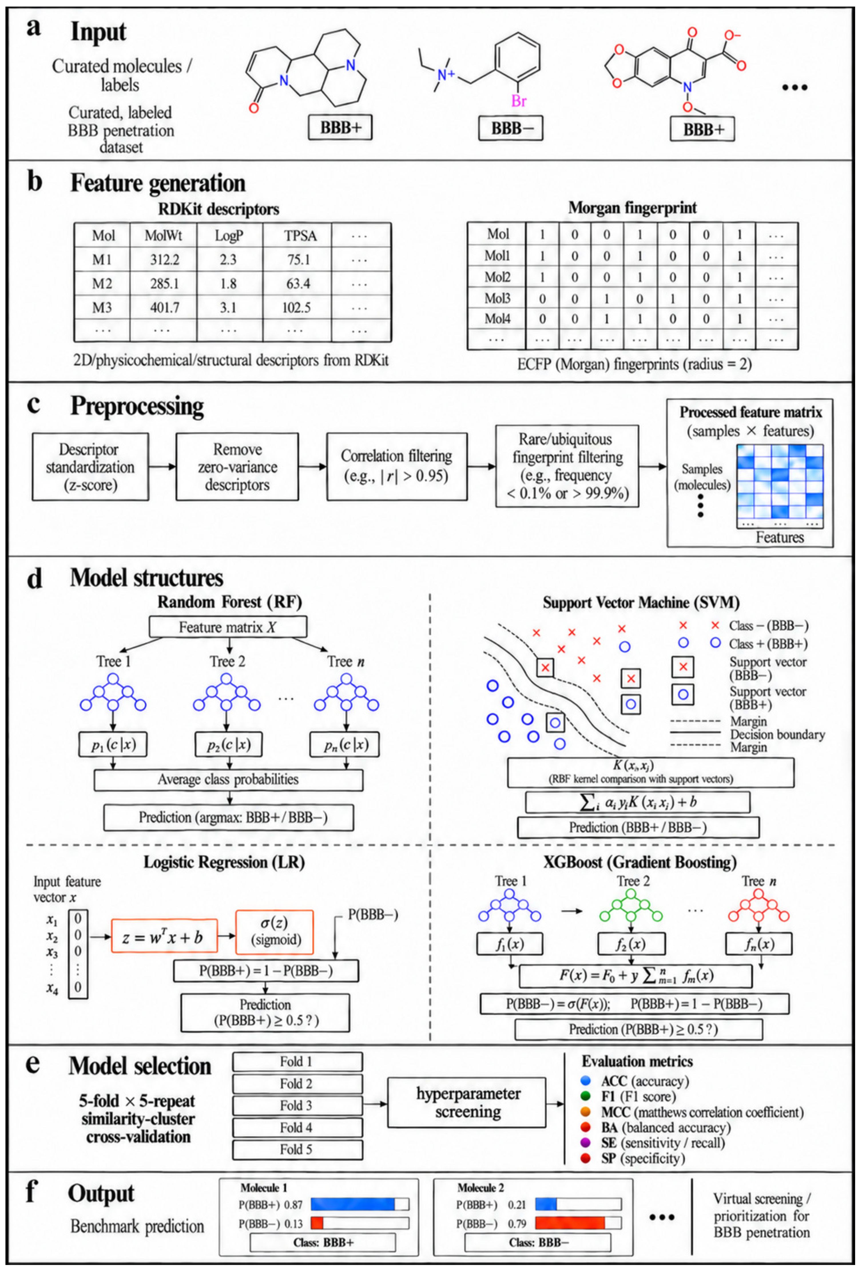
During the model-building phase (Figure 1), RDKit is used to generate Morgan fingerprints [34] with a radius of 2, a length of 2048 bits, and containing chiral information; the Tanimoto similarity is used to evaluate intermolecular structural similarity [35]. The Tanimoto similarity is defined as:
Figure 1.
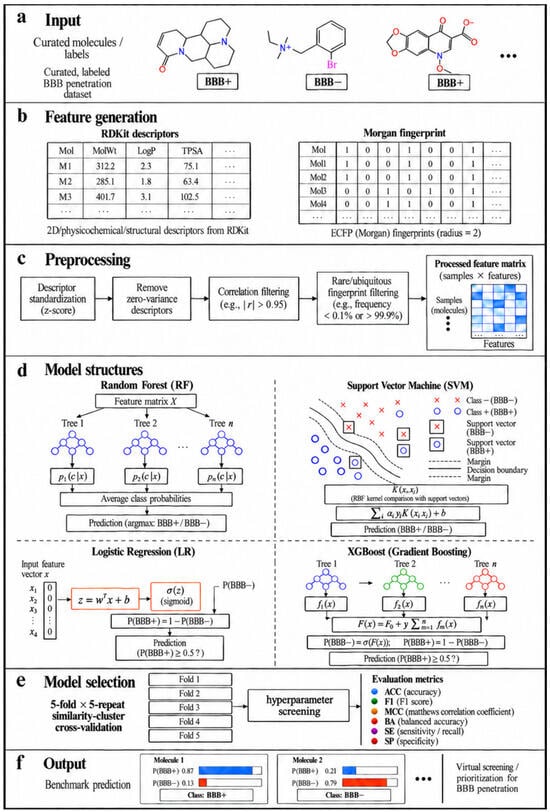
Machine learning workflow for blood–brain barrier permeability prediction. (a) Experimentally annotated molecules were curated and encoded as BBB+ or BBB−. (b) Molecular structures were converted into RDKit physicochemical and structural descriptors and Morgan fingerprints. (c) Preprocessing was fitted using training data only: descriptors were standardized, zero-variance descriptors were removed, highly correlated descriptors were filtered at |r| ≥ 0.95, and Morgan bits with prevalence below 0.1% or above 99.9% were excluded. (d) Random forest, support vector machine, logistic regression, and XGBoost classifiers were compared. (e) Model selection and parameter optimization were confined to the outer training partition using 5-fold × 5-repeat similarity-cluster CV; molecules connected at a Morgan Tanimoto similarity of ≥0.70 were kept within the same fold. ACC, F1, MCC, BA, SE, and SP were calculated, with mean MCC and BA prioritized for model selection. (f) The fixed 20% test set and the independent benchmark set were reserved for final evaluation.
In this equation, a and b represent the number of on bits in the fingerprints of the two molecules, respectively, and c is the number of on bits shared by both fingerprints.
During model execution, a “similarity-based near-duplicate filtering” process is first performed in memory. Within any given near-duplicate cluster, the Tanimoto similarity between molecules must be at least 0.95; for clusters with consistent labels, only a single representative molecule (the “cluster representative”) is retained, with priority given to retaining the quantitative representative molecule. Finally, clusters exhibiting label conflicts that cannot be resolved via quantitative data are discarded. Following this cleanup, compounds for which valid descriptors cannot be obtained are further removed.
Subsequently, the modeling subset undergoes stratified random splitting, with 80% designated as the outer training set and 20% as the fixed final test set. To mitigate data leakage caused by structurally similar molecules appearing in both training and validation folds, similarity clusters are constructed within the outer training set using a single-linkage approach with a Tanimoto similarity threshold of 0.70; this is followed by a 5-fold CV procedure based on these similar clusters, repeated five times.
2.2. Machine Learning Model Development and Comparison
The initial input for the traditional ML models consists of 208 RDKit 2D molecular descriptors and 2048-bit Morgan fingerprints. The RDKit descriptors characterize local or global features such as molecular weight, lipophilicity, topological polar surface area, and hydrogen-bond donor counts, while the Morgan fingerprints represent local chemical structural fragments within the molecules. During initial model development (Figure 1), we compared four classifiers: RF, SVM, logistic regression (LR), and XGB [36]. All four models employ the same outer training set and the same internal CV procedure (5-fold CV repeated 5 times). BBB+ was defined as the positive class and BBB− as the negative class. Evaluation was performed using accuracy (ACC), F1-score (F1), Matthews correlation coefficient (MCC) [37], balanced accuracy (BA), sensitivity (SE), and specificity (SP). The formulas for each metric are as follows:
In these equations, TP represents true positives, TN represents true negatives, FP represents false positives, and FN represents false negatives. ACC measures the proportion of correctly classified samples. The F1 combines precision and recall for the BBB+ class. The MCC considers TP, TN, FP, and FN together. It is therefore reliable for imbalanced datasets. BA gives equal weight to the two classes and evaluates their classification performance more evenly. SE, also called recall, measures the model’s ability to identify positive samples. SP measures the model’s ability to identify negative samples. For model selection, the mean MCC is used as the primary criterion, with the average BA serving as the secondary criterion. The fixed final test set and benchmark dataset are strictly excluded from model comparison, feature selection, and hyperparameter tuning.
2.3. XGBoost Feature Reduction and Hyperparameter Optimization
Prior to the dimensionality reduction experiments, a preliminary experimental phase was conducted, in which 10 descriptors were randomly selected from the 208 RDKit descriptors [38] and combined with 2048-bit Morgan fingerprints [34] in each trial; across 100 randomly sampled candidate inputs into the model, model performance declined to a certain extent. Subsequently, attempts were made to decrease the 2048-bit Morgan fingerprints to 1024 bits while retaining all 208 RDKit descriptors, whereas the fingerprints used for near-duplicate molecule cleaning, similarity cluster grouping, and applicability domain (AD) analysis remained fixed at 2048 bits. On the basis of ensuring performance, zero-variance descriptors in the training data were further removed, followed by retaining only one of the descriptors when the absolute value of the Pearson correlation coefficient between two descriptors was not less than 0.95; finally, Morgan bits with an occurrence frequency of less than 0.1% or greater than 99.9% in the training fold were removed. All filtering rules were independently determined within each CV training fold and then applied to the corresponding validation fold.
XGB hyperparameter optimization employs a two-stage search within the training set. In the first stage, 40 sets of candidate parameters are generated, including baseline parameters, combinations of single-parameter changes, and random parameter combinations generated using a fixed random seed. The parameters adjusted include the number of trees, maximum tree depth, learning rate, minimum child node weight, split loss threshold, row sampling rate, column sampling rate, L1 regularization coefficient, L2 regularization coefficient, and class weights. The 40 sets of candidate parameters first undergo a 5-fold CV on similar clusters. The candidate parameters and baseline parameters that perform well then proceed to the second stage, a full 5-fold CV repeated five times. In both stages, parameters are ranked primarily based on the average MCC, with the average BA used as a secondary selection criterion. The hyperparameter search spaces, evaluated configurations, and screening protocols are detailed in Table S5.
2.4. GNN Construction, Comparison, and Optimization
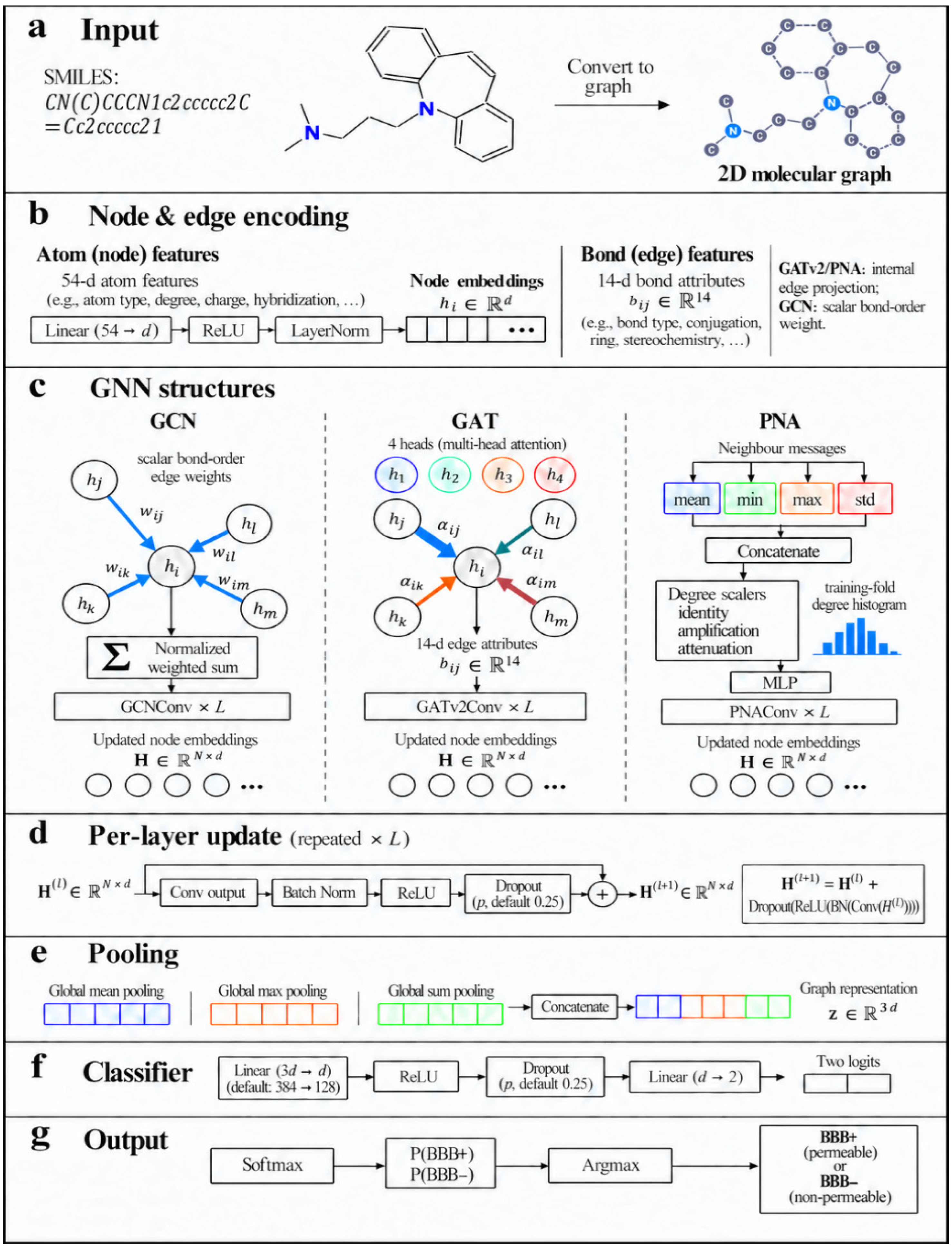
To compare traditional ML and deep learning methods, this study constructed three GNN architectures: GCN, GAT, and PNA. As shown in Figure 2, the GNN models take 2D molecular graphs directly as input, where atoms in a molecule are represented as nodes and each chemical bond is encoded as two directed edges in opposite directions. Each atom is characterized by a 54-dimensional node feature representation, including atomic number, atomic degree, and formal charge. Each chemical bond is characterized by a 14-dimensional edge feature representation, covering single bonds, double bonds, and aromatic bonds. All three architectures (Figure S1) incorporate node encoding, graph convolution, batch normalization, non-linear activation, residual connections, and dropout, and the molecular-level representations derived from global average pooling, max-pooling, and sum pooling are concatenated and fed into a fully connected classifier.
Figure 2.
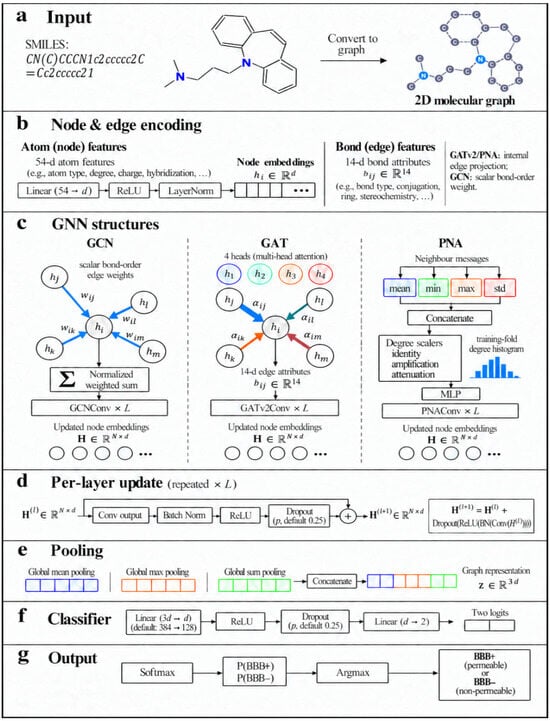
GNN workflow for blood–brain barrier permeability prediction. (a) Each SMILES string was parsed with RDKit and converted into a two-dimensional molecular graph. (b) Atoms were represented by 54-dimensional feature vectors encoding atom type, degree, formal charge, hydrogen count, valence, hybridization, chirality, aromaticity, ring membership, radical electrons, and atomic mass. Each chemical bond was represented by two directed edges with 14-dimensional features encoding bond type, conjugation, ring membership, and stereochemistry. (c) The GCN backbone used chemically defined scalar bond-order weights, GAT used multi-head GATv2 attention with full edge attributes, and PNA combined mean, minimum, maximum, and standard-deviation aggregators with identity, amplification, and attenuation degree scalers; the PNA degree histogram was estimated from each training fold only. (d) Every message-passing layer was followed by BatchNorm, ReLU, dropout, and a residual connection. (e) Global mean, maximum, and sum pooling were concatenated into a graph-level vector. (f) A multilayer perceptron generated two class logits, and (g) softmax probabilities and the maximum-probability class provided the BBB+ or BBB− prediction.
GCN converts different types of chemical bonds into corresponding scalar edge weights, where the weights for single, double, triple, and aromatic bonds are 1.0, 2.0, 3.0, and 1.5, respectively; the graph convolution approach is based on the classic GCN framework [39]. GAT employs a multi-head attention mechanism capable of processing edge features to learn the relative importance of different adjacent atoms and chemical bonds to the target atom [40]. PNA simultaneously utilizes four information aggregation methods—mean, minimum, maximum, and standard deviation—and combines three scaling methods—identity, amplification, and attenuation—to handle different node degrees [41]. The node degree distribution required by PNA is calculated solely from the current training fold, thereby preventing validation data from being used in network construction.
The three GNN architectures use the same outer training set, fixed test set, and similar cluster grouping as the ML models. Formal candidate confirmation at each stage was performed using 5-fold CV repeated five times, with the average MCC as the primary selection criterion and BA as a supplementary metric, while also examining the overall performance and class identification bias reflected by ACC, F1, SE, and SP. Within each CV training fold, a separate early-stopping subset isolated by similarity clusters was established, ensuring that the early-stopping process did not interact with the corresponding CV fold. Models were trained for a minimum of 30 epochs and a maximum of 300 epochs. Training was terminated when no improvement in results was observed for 30 consecutive epochs. The optimal number of epochs was determined sequentially based on the MCC, BA, and validation loss on the early-stopping subsets:
where e denotes the training epoch and Ebest denotes the selected optimal epoch. MCC was used as the primary criterion, BA as the secondary criterion, and validation loss as the final tie-breaking criterion.
After determining the optimal epoch, the model is reinitialized and trained for the same number of epochs on the complete CV training folds, followed by the calculation of the six-evaluation metrics on the validation folds that were not involved in early stopping. The final number of training epochs for the model is set to the median of the 25 best epochs from the selected architecture. The GNN uses the AdamW optimizer and weighted cross-entropy loss [42]. In subsequent GNN training, the BBB+ weight adjustment coefficient α is introduced to increase the contribution of BBB+ in the loss function, thereby improving the balance between SE and SP. For each training subset, inverse frequency weights are first calculated based on class frequencies, and then the loss contribution of BBB+ is adjusted using the coefficient α. The class weights for BBB+ and BBB− are expressed as follows:
In these equations, WBBB+ represents the weight of the BBB+ class in the cross-entropy loss function, and WBBB− represents the weight of the BBB− class in the cross-entropy loss function. N denotes the total number of samples in the current training subset. α denotes the weight adjustment coefficient for BBB+.
For the i-th sample, its weighted cross-entropy loss is:
In this equation, Li denotes the loss value generated by the i-th sample; Wyi denotes the class weight corresponding to the true class of that sample; and pi,yi denotes the predicted probability assigned by the model to the true class yi of the i-th sample, with values ranging from 0 to 1.
During training, GCN uses a BBB+ weight adjustment coefficient of 1.8, while GAT and PNA use 1.6. Gradient norms are clipped during training, and the learning rate is dynamically reduced based on the validation loss. Random seeds for Python (3.10.20), NumPy (1.26.4), PyTorch (2.11.0 + cu128), and CUDA (13.1) are all fixed, and deterministic computation is enabled to improve reproducibility across different training runs.
In the initial comparison, GCN, GAT, and PNA uniformly used a 128-dimensional hidden layer, 3 layers of graph convolutions, and a dropout rate of 0.25; GAT used 4 attention heads. Subsequently, architecture-specific adjustments were conducted, exploring hidden layer width, network depth, dropout probability, learning rate, weight decay, the number of GAT attention heads, and class weights.
In further hyperparameter screening, six sets of candidate configurations were set for each architecture, resulting in a total of 18 parameter sets for comparison. The initial screening employed 5-fold similar-cluster CV, with a maximum of 120 training epochs and a minimum of 15 epochs; training was terminated early if no performance improvement was observed for 15 consecutive epochs. The screening does not use a fixed final test set or benchmark; its sole purpose is to identify candidate configurations worthy of advancing to full repeated CV. The optimal candidate for each architecture must still be confirmed through the same 5-fold × 5-repetition similar-cluster CV before it can be used for final architecture selection and independent evaluation. The hyperparameter search spaces, evaluated configurations, and screening protocols are detailed in Tables S5–S7.
2.5. Protomer Sensitivity Analysis and Augmented Training
Using the original benchmark comprising 100 BBB+ and 100 BBB− compounds as the parent set, possible protomers were enumerated for each parent compound while retaining the mapping between parents and protomeric structures. Simultaneously, the protomeric structures inherited the binary classification labels of their parent compounds, and the formal charges calculated by RDKit were recorded, yielding a total of 962 enumerated ionization and tautomeric states. Each of the 962 enumerated ionization and tautomeric structures was individually input into the model to obtain its BBB+ probability, and binary classification was performed after calculating the average probability within each parent group. After the optimal model was selected in the preceding steps, this extended benchmark evaluation was conducted to test whether the model could maintain performance when applied to datasets characterized by multiple protonation states and diverse formal charges.
All molecular structures were parsed and validated for valence using RDKit; atomic formal charges and net formal charges were then calculated based on the molecular graphs. For entries that include charge annotations, the stated values were cross-checked against the recalculated net charges to ensure consistency. Structures with potential issues in their chemical representation were flagged for manual review.
No independent, state-specific experimental BBB permeability measurements were available for the enumerated protomers in this study. In both the training and benchmark expansions, each protomer inherited its parent compound’s reference BBB classification. This label inheritance served as an annotation assumption for representation-based augmentation and did not establish identical experimental permeability across individual states. Benchmark evaluation was performed at the parent level: predicted BBB+ probabilities were averaged without population weighting across the enumerated states of each parent, thresholded at 0.5, and compared with the original parent label. The six-performance metrics therefore assessed 200 parent-level predictions rather than 962 independently measured protomer outcomes.
Subsequently, protomer enumeration expansion was performed on the training set, and the corresponding ligand_id mapping was established according to the order of parent compounds in the original training table. RDKit was utilized to canonicalize the isomeric SMILES of parent compounds and protomers and recalculate their formal charges. Each valid parent compound was retained once, records in the protomer subset identical to their corresponding parent compounds in both canonical structure and formal charge were removed, and duplicate canonical SMILES within the same parent compound group were deleted. Conflicting permeability records sharing identical canonical structures across different parent compounds were removed, and invalid SMILES as well as structures generating non-finite descriptors were excluded. To maintain the integrity of the benchmark, overlap processing was consistently executed on the training data side, meaning that the original 200 parent compounds and 962 enumerated benchmark structures were preserved intact, whereas structures in the expanded training table that were completely identical to the expanded benchmark after canonicalization were removed. The optimized, newly expanded training set was used to retrain the selected models, whose performance was evaluated using the expanded benchmark. During retraining, the feature inputs, parameter settings, internal repeated CV, fixed test set, and evaluation metric calculations remained unchanged. Following retraining, the fixed test set and the 962 protomers corresponding to the original 200 parent compounds were evaluated separately and compared with the optimal model selected prior to protomer expansion to assess the effectiveness of incorporating protonation information into the model.
Protomer enumeration was performed using Epik Classic (version 7.6121; Schrödinger, LLC, New York, NY, USA) [32], integrated into Schrödinger LigPrep. Taking canonical SMILES as input, Epik Classic was invoked via LigPrep’s -epik option to generate possible ionization and tautomeric states at a target pH of 7.4 and a pH tolerance of 1.0, thereby examining molecular states potentially existing within the pH range of approximately 6.4–8.4. The enumeration results were output in SMILES format and mapped to their original parent compounds via a unique ‘ligand_id’.
3. Results and Discussion
3.1. Curation and Chemical-Space Characterization of the Modeling Dataset
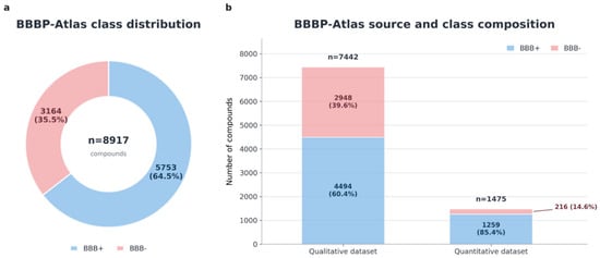
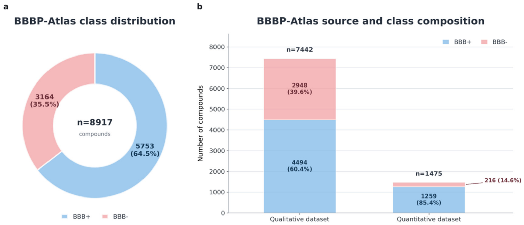
Curation of the qualitative and quantitative records from OmniBBBP resolved duplicate identities and conflicting annotations, prioritized quantitative records where the sources overlapped, and excluded benchmark overlaps. This yielded 8917 compounds with unique InChIKeys and canonical SMILES. Qualitative records constituted the larger source subset, and BBB+ compounds predominated overall, with stronger BBB+ enrichment in the quantitative subset (Figure 3). The proportion of BBB+ compounds is higher in the quantitative subset than in the qualitative subset, indicating that the two data sources differ in their compositional makeup. While this disparity does not, in itself, prove the existence of bias, the data coverage in literature compilations is contingent upon which compounds were selected for study, subjected to brain distribution analysis, and subsequently reported in the public domain; consequently, such datasets may be enriched with CNS-active drugs or compounds already flagged for their potential to penetrate the brain. The observed class distribution should therefore be interpreted as a reflection of the specific studies collected, rather than as the true ratio of BBB+ to BBB− compounds within the broader chemical space. Although structural de-duplication and similarity-based filtering help mitigate redundancy and data leakage, they cannot eliminate the representational limitations inherent in the initial selection of compounds for study. Furthermore, while a balanced benchmark facilitates the comparison of recognition capabilities across different categories, class balance does not equate to representativeness regarding the data source. Since this benchmark and the development data are drawn from the same integrated dataset, the results reflect performance on held-out compounds; they do not, by themselves, demonstrate that a model can generalize in an unbiased manner to unscreened candidate compound libraries.
Figure 3.
Class distribution and source composition of the curated BBBP-Atlas dataset before training-time similarity cleaning and data splitting. (a) Of 8917 compounds, 5753 (64.5%) were BBB+ and 3164 (35.5%) were BBB−. (b) The qualitative subset contained 7442 compounds, comprising 4494 BBB+ (60.4%) and 2948 BBB− (39.6%), whereas the quantitative subset contained 1475 compounds, comprising 1259 BBB+ (85.4%) and 216 BBB− (14.6%). The plot therefore shows both the moderate overall class imbalance and the stronger enrichment of BBB+ compounds in the quantitative source data.
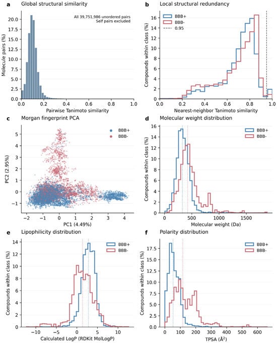
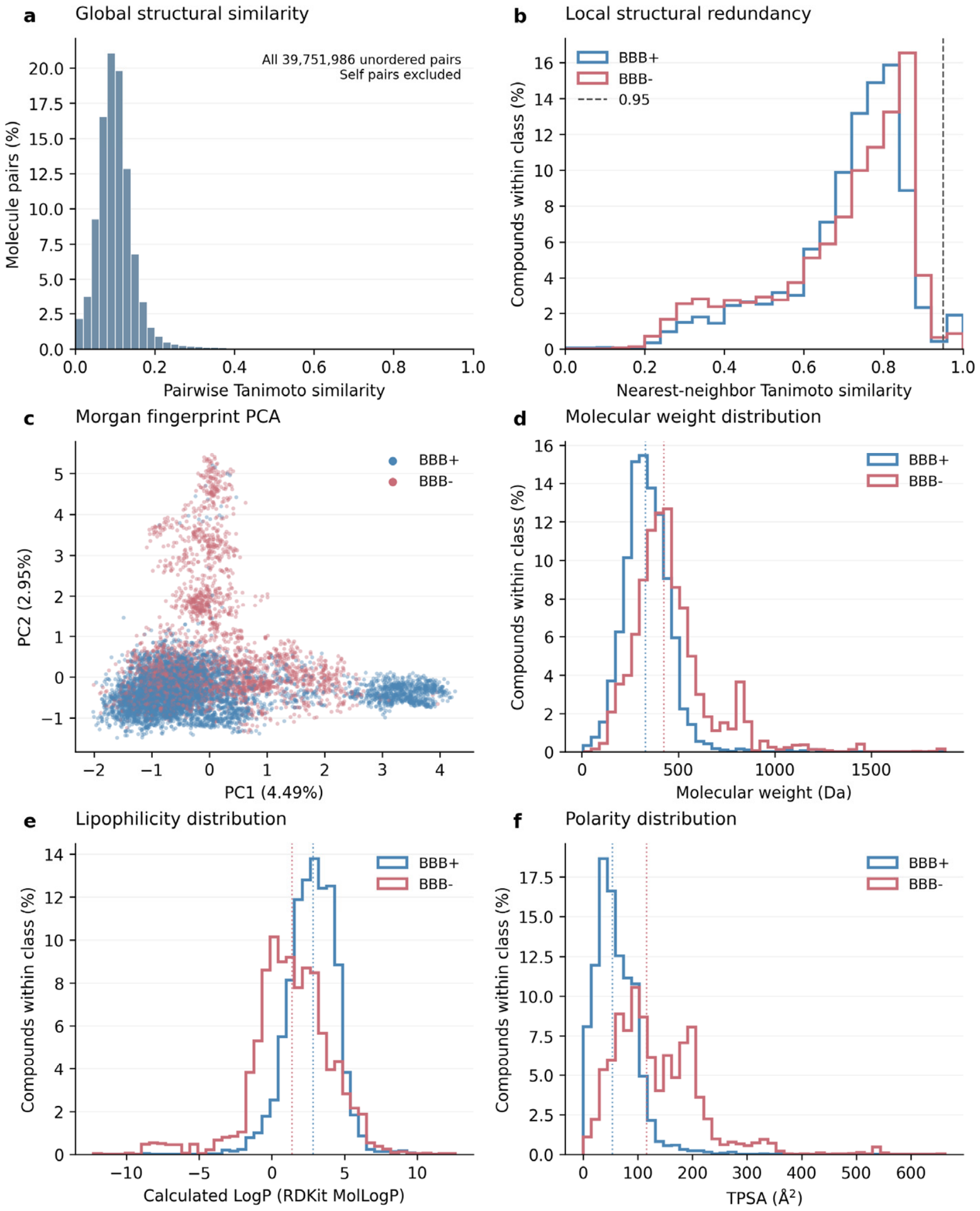
Chemical-space analysis of the curated parent dataset, prior to similarity-based filtering and protomer expansion, revealed substantial structural diversity, with a low median pairwise Tanimoto similarity (0.097) but a considerably higher median nearest-neighbor similarity (0.744; Figure 4a,b). These findings suggest broad structural heterogeneity alongside the presence of structurally related compounds. Principal component analysis (PCA) of Morgan fingerprints showed substantial overlap between BBB+ and BBB− compounds, with some localized class enrichment (Figure 4c). However, as the first two principal components explained only a small fraction of the total variance, the projection provides a qualitative overview of the chemical space.
Figure 4.
Chemical-space characterization of the curated parent dataset (n = 8917) before similarity-based filtering and protomer expansion. (a) Distribution of pairwise Tanimoto similarities among all unique molecular pairs. (b) Distribution of nearest-neighbor Tanimoto similarities, defined as the maximum similarity of each molecule to any other molecule in the dataset. Self-comparisons were excluded from both analyses, and similarities were calculated using chirality-aware Morgan fingerprints (radius = 2, 2048 bits). The dashed line in (b) marks the similarity threshold of 0.95 used for near-duplicate filtering. (c) Principal component analysis (PCA) projection of mean-centered Morgan fingerprints, with the explained variance indicated on each axis. Each point represents one molecule. (d–f) Distributions of molecular weight (MW), calculated lipophilicity (LogP), and topological polar surface area (TPSA), respectively. BBB+ and BBB− compounds are shown in blue and red, respectively. Histograms in (b,d–f) are normalized within each class, and dotted vertical lines in (d–f) indicate the corresponding class medians. All observed property values are retained.
The physicochemical distributions further revealed differences between BBB+ and BBB− compounds (Figure 4d–f). BBB+ compounds generally exhibited lower molecular weight and topological polar surface area (TPSA), along with higher calculated lipophilicity (LogP), than BBB− compounds. Nevertheless, the substantial overlap between the distributions highlights the physicochemical diversity of the dataset and indicates that these properties alone do not clearly separate the two classes.
Across the training set, fixed test set, and external benchmark datasets, BBB+ and BBB− molecules exhibited consistent differences in physicochemical properties, with TPSA showing a particularly pronounced difference between the two classes. Overall, BBB+ molecules tended to have lower molecular weights, lower polarity, fewer hydrogen-bond donors and acceptors, and higher calculated LogP values (Figure S2). In contrast, BBB− molecules were more likely to violate multiple Lipinski’s rule of five (Ro5) thresholds (Table S10). These findings highlight the association between physicochemical properties and BBBP classification, although substantial overlap between the classes remains.
Following training-time near-duplicate filtering and exclusion of structures with non-finite descriptors, the final modeling dataset contained 8836 compounds. Fixed stratified splitting yielded 7068 outer-training compounds and 1768 final-test compounds while preserving the overall class balance. The outer-training set was organized into 4047 similarity clusters for subsequent repeated grouped CV.
In this study, logBB > −1 was adopted as an operational threshold for consistent BBB classification rather than as an indicator of favorable brain exposure for CNS drug development. As logBB represents the logarithm of the ratio of total brain concentration to total blood or plasma concentration, this threshold corresponds to a concentration ratio greater than 0.1 but does not necessarily indicate sufficient unbound drug exposure in the brain to achieve a pharmacological effect. Moreover, total brain distribution is influenced by tissue binding, blood or plasma protein binding, and active transport processes, and therefore does not directly measure passive permeability across the blood–brain barrier. Integrating qualitative BBB annotations with thresholded logBB measurements broadens the chemical coverage of the dataset but does not eliminate heterogeneity in experimental endpoints and measurement conditions. Differences in reference matrices (whole blood versus plasma), sampling times, and steady-state conditions may affect the reported distribution ratios, while qualitative BBB annotations may be based on different experimental criteria. Therefore, the combined dataset was used for BBB classification without assuming that all records represent equivalent measurements of passive permeability. The reported model performance reflects predictions under this integrated labeling framework, and further validation using independent datasets with well-defined experimental conditions remains necessary.
3.2. Comparison of ML Models and BBBP-Atlas
XGB provided the strongest balanced discrimination among the four traditional ML models under the shared internal validation protocol and was selected for further optimization (Table 1). RF favored BBB+ sensitivity at the expense of specificity, whereas XGB offered a more favorable balance between the two classes. This distinction supports model selection based on MCC and BA rather than sensitivity alone.
Table 1.
Internal CV comparison of baseline ML models and XGBoost feature sets. Bold values indicate the best performance for each evaluation metric.
Reducing the Morgan fingerprint from 2048 to 1024 bits and subsequently filtering the RDKit descriptors from 208 to 173 preserved essentially the same internal CV performance (Table 1). Thus, the smaller feature set retained predictive performance while reducing input redundancy; dimensionality reduction alone did not produce a marked improvement in classification.
Hyperparameter tuning mainly improved specificity and balanced discrimination, with only a modest change in overall accuracy. The full and filtered descriptor sets performed similarly under the selected settings (Table 2). The more compact 173-descriptor + 1024-bit fingerprint representation was therefore retained; the selected hyperparameters are listed in Table S3.
Table 2.
Two-tuned XGBoost and BBBP-Atlas performance comparison. Bold values indicate the best performance for each evaluation metric.
The selected XGB model retained strong predictive performance on the fixed test set and the external benchmark (Table 2). Benchmark performance was lower than test-set performance, emphasizing the need for an external assessment in addition to internal model selection. The model choice was determined from internal validation before these evaluation results were examined.
On the balanced external benchmark, XGB performed comparably to the reported BBBP-Atlas model, with the same sensitivity and small numerical advantages in several other metrics (Table 2). These results demonstrate the competitiveness of the descriptor-based approach under the present evaluation conditions, without implying overall superiority over the deep-learning model.
3.3. Comparison and Optimization of Three GNN Architectures
GNN development progressed from a shared initial configuration through PNA capacity reduction, class-weight adjustment, and architecture-specific hyperparameter screening. This sequence distinguished changes in network capacity from changes in the balance of class-specific errors.
Under the shared initial configuration, GAT ranked highest by MCC and BA, although PNA achieved the highest accuracy (Table 3). Specificity exceeded sensitivity for all three architectures, indicating stronger recognition of BBB− than BBB+ compounds. Accuracy alone therefore did not identify the most balanced candidate.
Table 3.
Internal CV comparison of initial GNN architectures and capacity-reduced PNA. Bold values indicate the best performance for each evaluation metric.
Reducing PNA capacity modestly improved MCC and BA, but further increased specificity while reducing sensitivity (Table 3). A smaller network therefore improved some summary metrics without resolving the initial imbalance in class recognition.
Class-weight adjustment increased BBB+ sensitivity in GCN and GAT and brought their class-specific recall rates into closer balance (Table 4). PNA showed little change at this stage, and GAT remained the strongest candidate by mean MCC. The differing responses indicate that loss weighting and network architecture needed to be considered together.
Table 4.
Internal CV performance of GNN architectures after class weighting. Bold values indicate the best performance for each evaluation metric.
Architecture-specific screening identified promising configurations for each backbone, including a lightweight PNA. Because screening used a single grouped 5-fold run, its rankings were treated as provisional and the selected configurations were evaluated again using the full repeated CV protocol.
In the repeated CV confirmation, PNA achieved the highest mean MCC and BA and the closest balance between sensitivity and specificity (Table 5). GCN and GAT had slightly higher F1 scores but less balanced class-specific recall. The preferred architecture consequently changed from GAT in the earlier stages to PNA after architecture-specific optimization.
Table 5.
Internal CV performance of GNN architectures after hyperparameter tuning. Bold values indicate the best performance for each evaluation metric.
PNA was selected as the representative GNN using internal validation, before the fixed test and benchmark results were examined. The final outer-training fit used 33 epochs, the median fold-specific stopping epoch. This provided a common final-training rule without selecting the epoch on either evaluation set.
3.4. Comparison of Final Model Performance Across Structural Similarity Levels
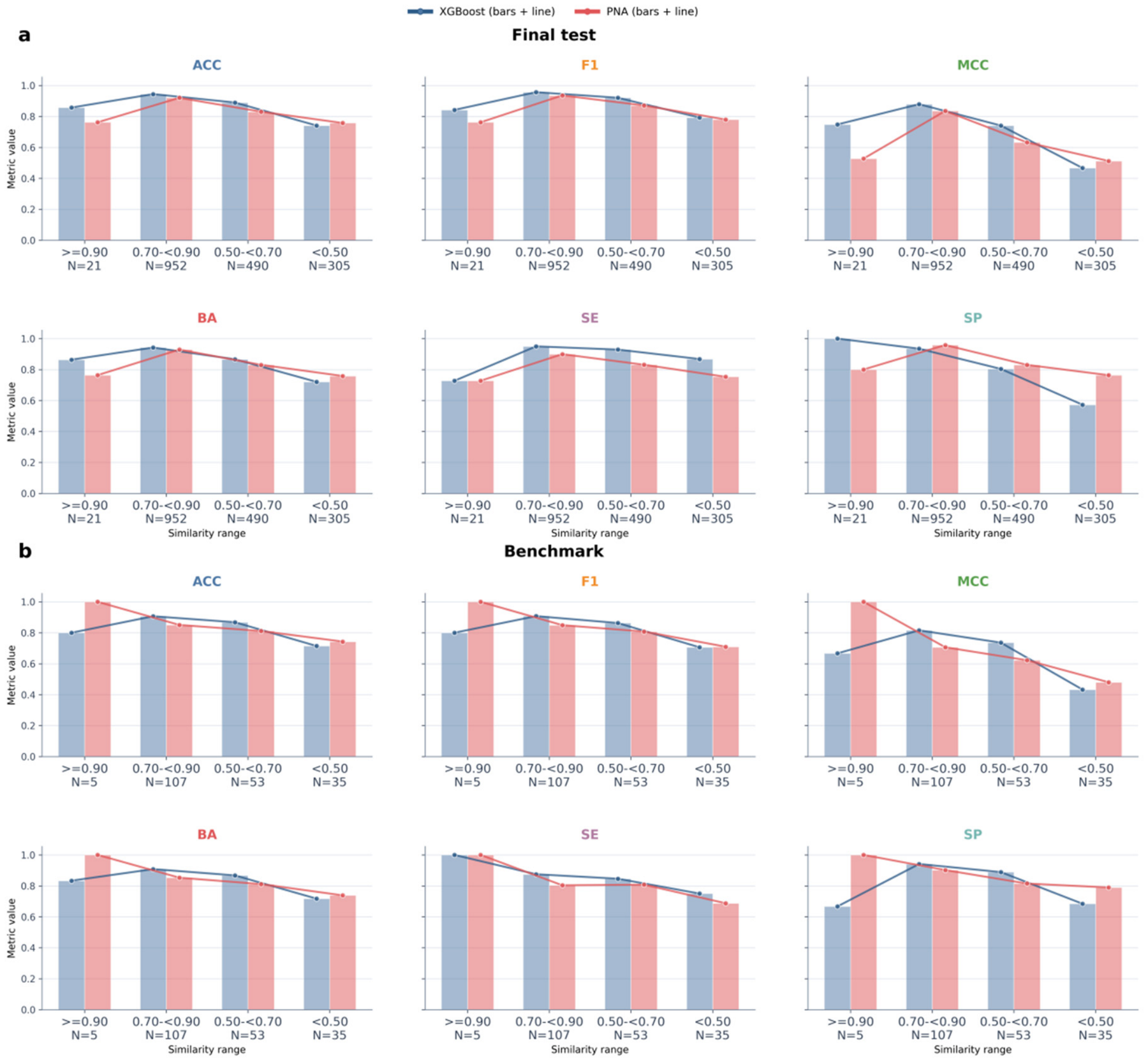
The optimized XGB outperformed the representative PNA overall on both evaluation sets. The fixed-test MCCs were 0.765 and 0.720, respectively, and the benchmark MCCs were 0.720 and 0.652 (Table S1). PNA nevertheless had higher specificity on the fixed test set, showing that the models differed in their error profiles rather than simply shifting all metrics together.
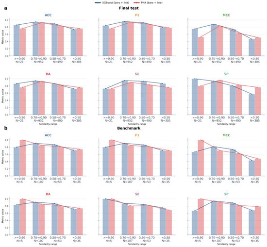
Similarity stratification showed that both models performed less well on compounds most dissimilar to the outer-training set (Figure 5; Table S1). The well-represented intermediate-to-high similarity strata generally supported stronger predictions, whereas the low-similarity stratum exposed a greater dependence on model architecture.
Figure 5.
Similarity-stratified comparison of the tuned 173 + 1024 XGBoost and optimized PNA models. Performance is shown for (a) the fixed final test set and (b) the independent 200-compound benchmark set. For each molecule, similarity was defined as the maximum Tanimoto coefficient to the outer-training reference calculated from chirality-aware, radius-2, 2048-bit Morgan fingerprints. Molecules were grouped into ≥0.90, 0.70–<0.90, 0.50–<0.70, and <0.50 strata; the number of molecules in each stratum is shown below the x-axis. Bars and overlaid lines display the same ACC, F1, MCC, BA, SE, and SP values for XGBoost (blue) and PNA (red). XGBoost was generally superior in the medium- and high-similarity strata, whereas PNA showed higher ACC, MCC, BA, and SP in the <0.50 strata, accompanied by lower SE. The decline observed for both models at low similarity reflects the greater difficulty of predicting chemically dissimilar compounds.
For compounds with maximum training-set Tanimoto similarity below 0.50, PNA achieved higher ACC, MCC, BA, and specificity than XGB in both the fixed test and benchmark subsets (Figure 5). This advantage was accompanied by lower sensitivity, indicating better recognition of BBB− compounds rather than a uniform improvement across both classes.
Additional fixed-test analysis confirmed that low training-set similarity was associated with more prediction errors. The main loss was in BBB− recognition, rather than an equivalent decline in both class recalls. Correct predictions nevertheless remained common among the low-similarity molecules, so the existing 0.50 cutoff should be interpreted as a cautionary stratum rather than a deterministic boundary between correct and incorrect predictions. The secondary training-derived threshold identified a more structurally remote subset with a further reduction in performance (Table S8).
The model’s applicability is constrained by the structural and physicochemical coverage of the training data. Low structural similarity to the training set indicates limited empirical support, and a high predicted probability does not necessarily imply a reliable prediction. The additional nearest-neighbor similarity threshold, derived exclusively from the training data without using test labels, serves as a structural-domain diagnostic rather than a validated applicability domain (AD). Molecular weight, calculated LogP, and TPSA provide complementary information on physicochemical coverage, but their individual ranges cannot capture sparsely represented regions or unfamiliar combinations of molecular properties. Notably, all fixed-test compounds fell within the corresponding training ranges, despite differences in prediction performance. Therefore, predictions for compounds with limited training support should be interpreted cautiously and subjected to further evaluation. Establishing a comprehensive, validated multivariate AD remains an important direction for future work.
3.5. Impact of Protomer Representation on Model Predictions and the Effect of Expanded Retraining
Enumeration expanded the 200 benchmark parents into 962 protomeric structures. After deduplication, benchmark-overlap exclusion, and separation of the fixed test parents and their protomers, the expanded training set comprised 34,671 unique structures.
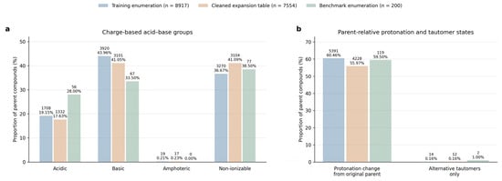
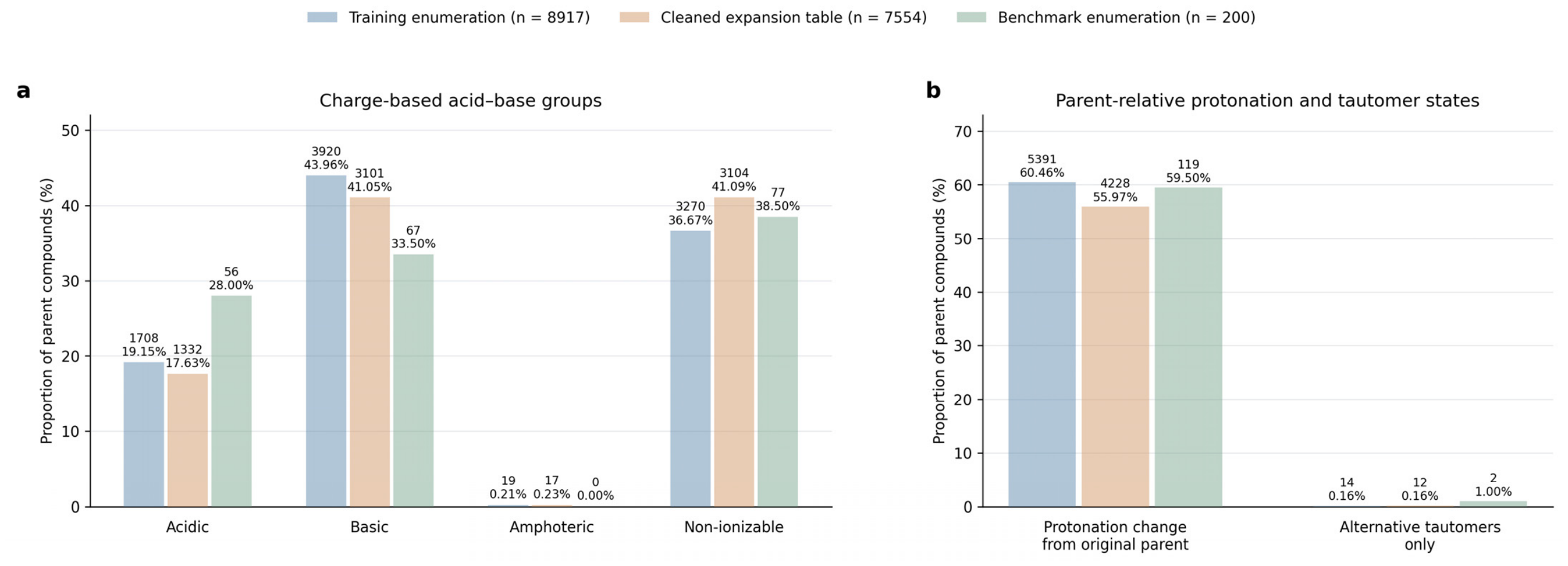
Analysis of the enumerated structures showed that basic and non-ionizable compounds predominated in the training set, whereas acidic compounds were relatively more prevalent in the benchmark and amphoteric compounds were uncommon (Figure 6a). The overall acid–base group composition remained largely unchanged after data cleaning. Comparison with the original parent structures further revealed that approximately three-fifths of compounds in both the training and benchmark sets generated at least one enumerated state with a different net charge, with a slightly lower proportion observed after cleaning. In contrast, only a small fraction of parent compounds generated alternative tautomers without a change in net charge relative to the original structure (Figure 6b). In the parent-level evaluation of the expanded benchmark, protomer-expanded training improved MCC from 0.607 to 0.658 in the charge-defined ionizable subset, compared with a smaller increase from 0.738 to 0.763 in the non-ionizable subset. These findings suggest a greater performance improvement among compounds exhibiting alternative charge states.
Figure 6.
Charge-based composition and parent-relative protonation-state changes in the enumerated datasets. (a) Proportions of compounds classified as acidic, basic, amphoteric, or non-ionizable based on their enumerated charge states. (b) Proportions of parent compounds generating at least one enumerated state with a net charge different from the original parent structure, or generating only alternative tautomers without a change in net charge relative to the parent.
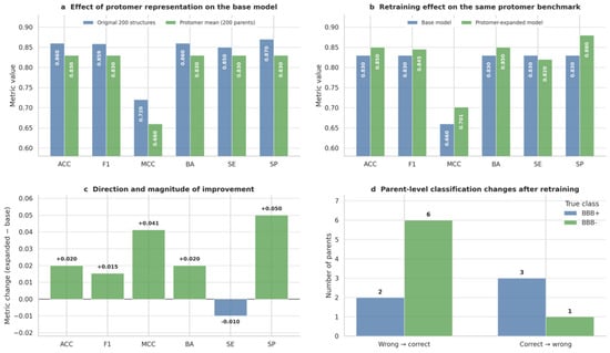
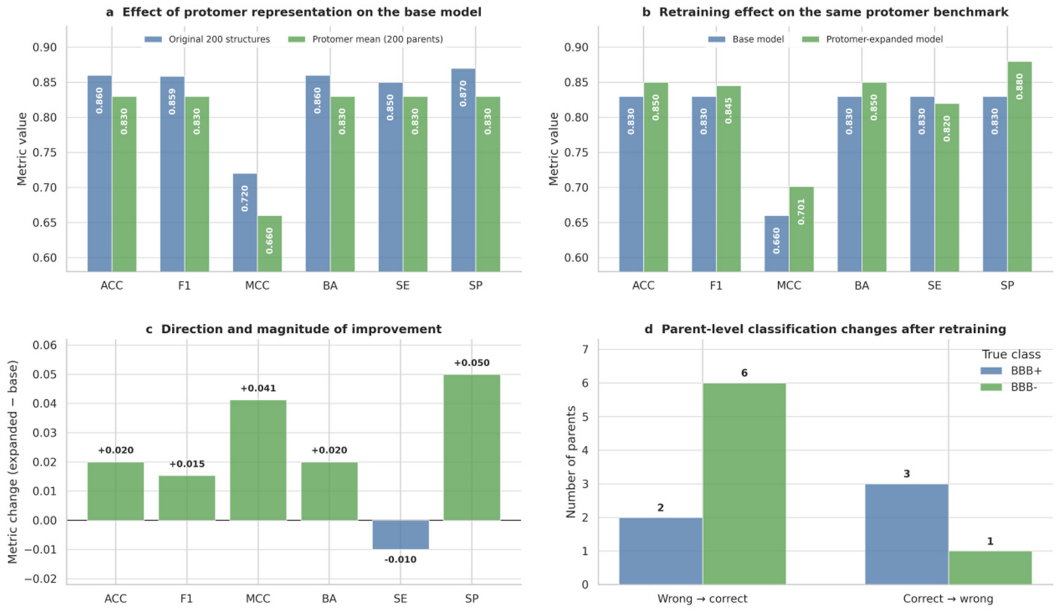
Applying the baseline XGB to alternative protomer representations reduced parent-level benchmark performance relative to the original input structures (Figure 7a). MCC decreased from 0.720 to 0.660, showing that changing the representation of the same parents could alter classification performance without changing their reference labels.
Figure 7.
Effect of protomer representation and protomer-expanded retraining on the benchmark set. The 200 benchmark parent compounds were expanded to 962 protomer structures, and parent-level predictions were obtained by averaging P(BBB+) across all protomers assigned to the same ligand ID; a threshold of 0.5 was then used for classification. (a) Performance of the original tuned 173 + 1024 XGBoost model on the 200 original parent structures versus parent-mean predictions from their enumerated protomers. (b) On the same protomer-expanded benchmark, retraining the XGBoost model with the protomer-expanded training set. (c) Metric differences between the expanded and base models summarize the direction and magnitude of these changes. (d) At the parent level, retraining corrected eight predictions (two BBB+ and six BBB−, see Table S2), but changed four previously correct predictions to incorrect ones (three BBB+ and one BBB−). These results indicate a net improvement, driven primarily by better recognition of BBB− parents.
Protomer-expanded retraining partly recovered this loss, increasing parent-level MCC to 0.701 (Figure 7b,c). The gain was driven mainly by improved specificity, with a slight decrease in sensitivity. Internal CV and fixed-test performance remained close to the base model rather than improving uniformly (Table S4). Retraining corrected more parent predictions than it disrupted, with most corrections occurring among BBB− parents (Figure 7d). Thus, the main benefit was improved robustness to enumerated representations, not an across-the-board increase in predictive performance.
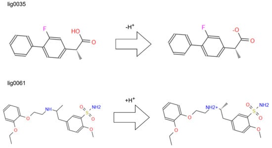
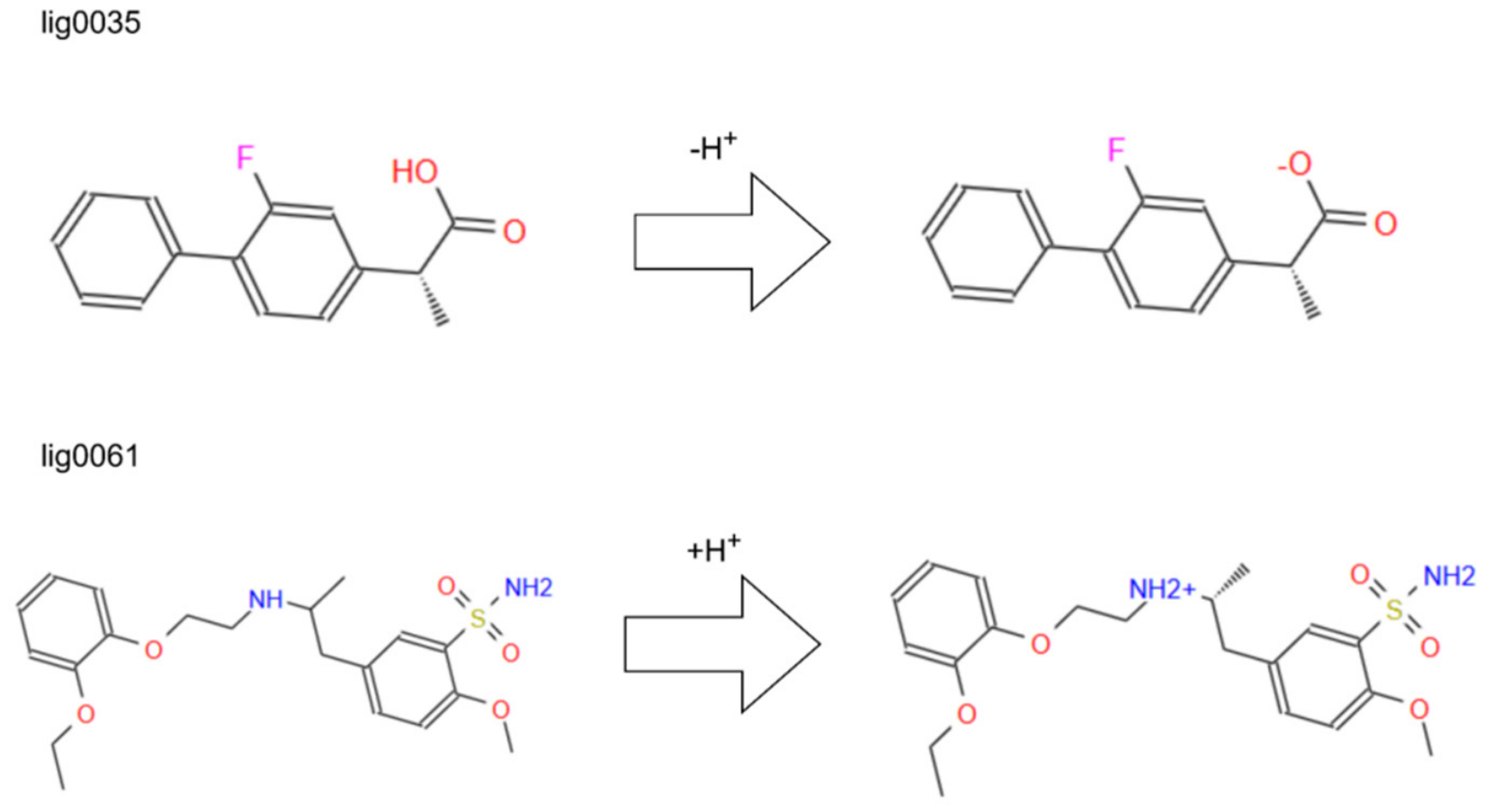
The corrected predictions for lig0035 and lig0061 illustrate this change in model behavior (Figure 8; Table S2). The former was represented by a deprotonated carboxylate and the latter by a protonated amine; both are BBB− compounds. For the same enumerated structures, retraining shifted their predicted BBB+ probabilities across the classification threshold in the correct direction. These examples illustrate changes in the model’s response to ionized molecular representations rather than providing experimental evidence that protonation necessarily reduces BBB permeability.
Figure 8.
Representative charge-state transformations associated with corrected benchmark predictions after protomer-expanded retraining. Ligand IDs were assigned according to the row order of the original benchmark, and all enumerated protomers inherited the corresponding parent ID. For lig0035 (upper), deprotonation of the carboxylic acid generated a carboxylate and changed the net formal charge from 0 to −1; the charge-specific P(BBB+) decreased from 0.659 with the base model to 0.425 with the protomer-expanded model. For lig0061 (lower), protonation of the secondary amine generated an ammonium center and changed the net formal charge from 0 to +1; P(BBB+) decreased from 0.831 to 0.417. Both compounds were experimentally labelled BBB−, so the probability shifts crossed the 0.5 threshold and corrected the classifications.
The observed improvement should be interpreted in the context of the augmentation strategy. Protomer-expanded training altered molecular representation coverage as well as the size and composition of the training set, making it difficult to isolate the contribution of charge alone. Furthermore, the enumerated protomers inherited their parent-compound labels, and their predicted probabilities were averaged without accounting for physiological state populations. As state-specific pKa estimates and relative populations at pH 7.4 were not available in the present Epik Classic workflow, population-weighted evaluation could not be performed. Therefore, these findings suggest improved robustness to alternative molecular representations rather than experimentally validated permeability differences among individual protonation states. Future work could incorporate predicted pKa values and physiological protonation-state populations to further investigate the influence of ionization on BBBP predictions.
3.6. Sensitivity to the logBB Classification Boundary and Training Labels
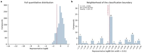
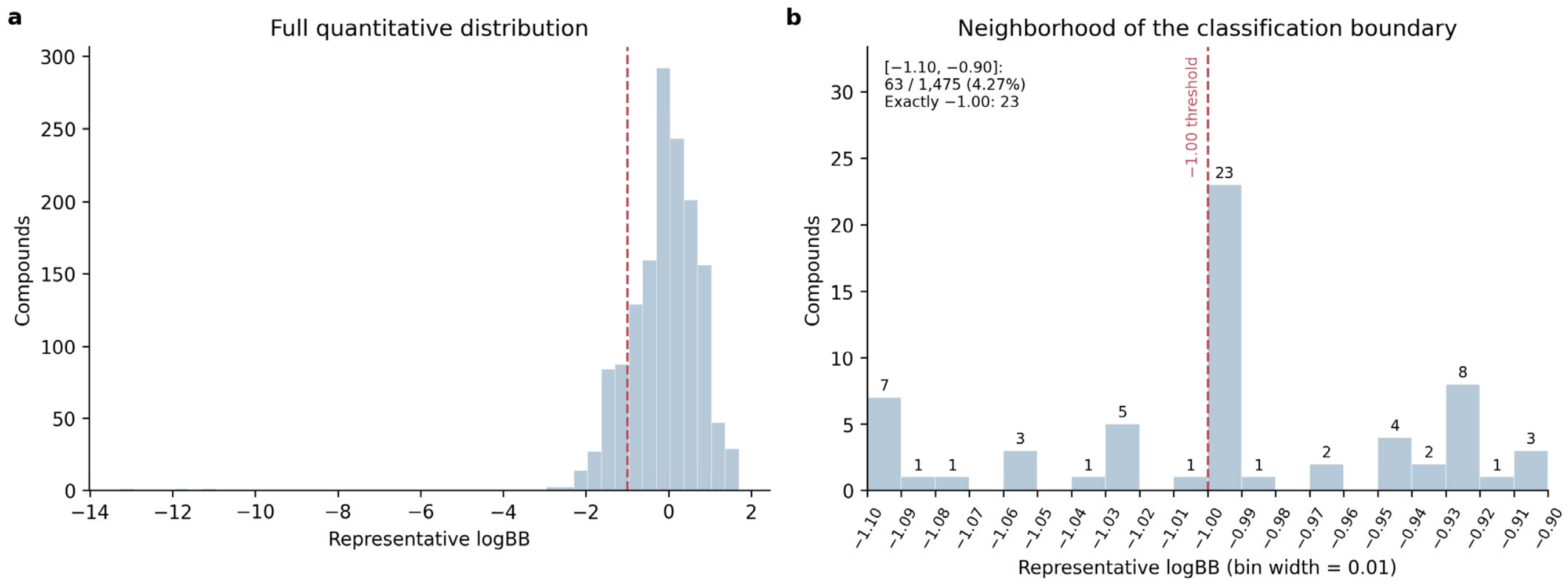
Using a fixed logBB threshold allows quantitative records to be incorporated into a unified binary classification task. However, small numerical differences near the threshold can result in opposite labels, an inherent limitation of the training labels used by this model. To investigate this boundary effect, we first analyzed the logBB distribution in the integrated quantitative dataset, focusing on the local distribution around −1 (Figure 9). In this interval, records classified as “BBB−” accounted for 19.44% of all quantitative “BBB−” entries. Although this proportion was relatively small overall, its impact on the minority class warrants further investigation.
Figure 9.
Distribution of logBB values in the curated quantitative subset (n = 1475). (a) Overall distribution of representative logBB values. (b) Enlarged view of the classification boundary (logBB = −1.00), showing values within the interval [−1.10, −0.90] using a bin width of 0.01.
Next, we adjusted the threshold for the “BBB+” classification in the quantitative training data from logBB > −1 to logBB > −1.01 to assess the model’s sensitivity to local perturbations in the training labels. This adjustment changed the classifications of 17 molecules with logBB values exactly equal to −1 from “BBB−” to “BBB+”; these data accounted for 0.24% of the entire training set. The qualitative labels, final test set, and benchmark reference labels remained unchanged. We then retrained the model on this revised dataset and reevaluated it against the benchmark. We also considered a threshold of −0.99. However, because no compounds in the quantitative training set had logBB values in the range −1 < logBB ≤ −0.99, this threshold would not change any training labels. Accordingly, no additional model training was needed for this scenario because it introduced no new perturbation.
When evaluated on the same 200 benchmark compounds, the model’s MCC and other performance metrics showed a slight decline (Table 6). Classification results remained unchanged for 198 compounds, while the classifications of the other 2 changed from correct to incorrect. Overall, this local perturbation of the training labels did not substantially affect benchmark classification results, but it also indicates that the model is not entirely insensitive to labels in borderline cases. Within the range of this adjustment, from −1 to −1.01, the model showed some classification robustness while remaining sensitive to labels near the threshold. Future studies, including the incorporation of measurement conditions and error data and expansion of the sensitivity analysis, will help more accurately characterize the extent to which label uncertainty affects the model’s conclusions.
Table 6.
Benchmark performance under training-label threshold perturbation.
4. Conclusions
This study established a BBBP classification workflow that integrates data cleaning and leakage control, comparisons between traditional ML and GNNs, similarity-based evaluation, and protomer sensitivity analysis. Among the models evaluated, XGB using 173 selected RDKit descriptors and a 1024-bit Morgan fingerprint showed the strongest overall performance, achieving MCC values of 0.765 on the fixed test set and 0.720 on the external benchmark. Its performance was comparable to that reported for BBBP-Atlas (MCC of 0.700), supporting the continued competitiveness of descriptor- and fingerprint-based ML for medium-scale BBBP prediction. Although the lightweight PNA model did not outperform XGB overall, its performance on low-similarity subsets demonstrated its complementary value.
The protonation-state analysis further showed that BBBP predictions can be sensitive to alternative molecular representations. When predictions were evaluated across enumerated protomeric states, model performance decreased relative to evaluation using the original structures, whereas retraining with protomer-expanded data partially recovered this loss, increasing the parent-level MCC from 0.660 to 0.701. These results indicate that protomer-expanded training can improve robustness to protonation-state variation. Overall, the findings highlight the importance of data quality, structural leakage control, and molecular representation in BBBP model evaluation. Future work should incorporate physiologically weighted protonation states and statistical uncertainty analysis to further assess model generalizability and representation robustness.
Supplementary Materials
The following supporting information can be downloaded at: https://www.mdpi.com/article/10.3390/molecules31224164/s1, Table S1. Overall and similarity-stratified predictive performance of the tuned 173-descriptor + 1024-bit Morgan-fingerprint XGBoost model and the optimized PNA model on the fixed final test set and the independent 200-compound benchmark set. Table S2. Charge-specific BBB+ probabilities for benchmark parent compounds whose initially incorrect parent-level predictions were corrected after protomer-expanded XGBoost retraining. Table S3. Selected XGBoost yperparameters. Table S4. Evaluation of base and protomer-expanded XGBoost models. Table S5. Discrete XGBoost hyperparameter search space. Table S6. Architecture-specific GNN search values. Table S7. Exact GNN configurations evaluated in initial HPO screening. Table S8. Fixed-test performance under structural-similarity diagnostics. Table S9. Illustrative low-similarity test predictions and their closest training references. Table S10. Rule-of-Five violation counts by dataset and permeability class. Figure S1. Architectures of the optimized (a) graph convolutional network (GCN), (b) graph attention network (GAT), and (c) principal neighbourhood aggregation (PNA) classifiers. Figure S2. Physicochemical distributions of BBB+ and BBB− compounds across the frozen training (n = 7068), fixed final-test (n = 1768) and original external-benchmark (n = 200) sets.
Author Contributions
Conceptualization, P.X. and C.Y.; methodology, B.X., D.Y., X.D., P.X. and C.Y.; software, B.X. and D.Y.; validation, B.X., D.Y. and X.D.; formal analysis, B.X., D.Y. and X.D.; investigation, B.X., D.Y. and X.D.; data curation, B.X.; visualization, B.X.; writing—original draft preparation, B.X.; writing—review and editing, B.X. and C.Y.; supervision, P.X. and C.Y.; project administration, P.X. and C.Y. All authors have read and agreed to the published version of the manuscript.
Funding
This research received no external funding.
Institutional Review Board Statement
Not applicable.
Informed Consent Statement
Not applicable.
Data Availability Statement
The datasets and code used in this study are publicly available. The BBBP workflow and source code are available at GitHub (3.22.1) at www.github.com/xiebc66/BBBP-Prediction-ML-DL-workflows (accessed on 29 September 2026). The BBBP datasets analyzed in this study were obtained from publicly available datasets as described in the Section 2. Data processing and model development were performed in a Python 3.10.20 conda environment. Traditional machine learning analyses primarily used RDKit 2022.09.5, NumPy 1.26.4, pandas 2.1.4, SciPy 1.11.4, scikit-learn 1.3.2, and XGBoost 3.2.0. Results were visualized using Matplotlib 3.7.5 and Seaborn 0.13.2. The graph neural network models were implemented using PyTorch 2.11.0 + cu128, PyTorch Geometric 2.8.0.post1, and torch-scatter 2.1.2 + pt211cu128. Protomer enumeration was performed using Epik Classic (version 7.6121; Schrödinger, LLC, New York, NY, USA), integrated into Schrödinger LigPrep.
Acknowledgments
The authors acknowledge the Shenzhen AI-Driven Public Service Platform for Pharmaceutical R&D (XMHT20251128002) for providing research support and computational resources. We thank Schrödinger for a license to LigPrep.
Conflicts of Interest
The authors declare no conflicts of interest.
References
- Pardridge, W.M. The blood-brain barrier: Bottleneck in brain drug development. NeuroRx 2005, 2, 3–14. [Google Scholar] [CrossRef] [Scilit]
- Abbott, N.J.; Patabendige, A.A.; Dolman, D.E.; Yusof, S.R.; Begley, D.J. Structure and function of the blood–brain barrier. Neurobiol. Dis. 2010, 37, 13–25. [Google Scholar] [CrossRef] [Scilit] [PubMed]
- Daneman, R.; Prat, A. The blood–brain barrier. Cold Spring Harb. Perspect. Biol. 2015, 7, a020412. [Google Scholar] [CrossRef] [Scilit] [PubMed]
- Rankovic, Z. CNS drug design: Balancing physicochemical properties for optimal brain exposure. J. Med. Chem. 2015, 58, 2584–2608. [Google Scholar] [CrossRef] [Scilit] [PubMed]
- Martins, I.F.; Teixeira, A.L.; Pinheiro, L.; Falcao, A.O. A Bayesian approach to in silico blood-brain barrier penetration modeling. J. Chem. Inf. Model. 2012, 52, 1686–1697. [Google Scholar] [CrossRef] [Scilit] [PubMed]
- Meng, F.; Xi, Y.; Huang, J.; Ayers, P.W. A curated diverse molecular database of blood-brain barrier permeability with chemical descriptors. Sci. Data 2021, 8, 289. [Google Scholar] [CrossRef] [Scilit] [PubMed]
- Kumar, R.; Sharma, A.; Alexiou, A.; Bilgrami, A.L.; Kamal, M.A.; Ashraf, G.M. DeePred-BBB: A blood brain barrier permeability prediction model with improved accuracy. Front. Neurosci. 2022, 16, 858126. [Google Scholar] [CrossRef] [Scilit] [PubMed]
- Mensch, J.; Oyarzabal, J.; Mackie, C.; Augustijns, P. In vivo, in vitro and in silico methods for small molecule transfer across the BBB. J. Pharm. Sci. 2009, 98, 4429–4468. [Google Scholar] [CrossRef] [Scilit] [PubMed]
- Wu, Z.; Ramsundar, B.; Feinberg, E.N.; Gomes, J.; Geniesse, C.; Pappu, A.S.; Leswing, K.; Pande, V. MoleculeNet: A benchmark for molecular machine learning. Chem. Sci. 2018, 9, 513–530. [Google Scholar] [CrossRef] [Scilit] [PubMed]
- Shaker, B.; Yu, M.-S.; Song, J.S.; Ahn, S.; Ryu, J.Y.; Oh, K.-S.; Na, D. LightBBB: Computational prediction model of blood–brain-barrier penetration based on LightGBM. Bioinformatics 2021, 37, 1135–1139. [Google Scholar] [CrossRef] [Scilit] [PubMed]
- Mazumdar, B.; Sarma, P.K.D.; Mahanta, H.J.; Sastry, G.N. Machine learning based dynamic consensus model for predicting blood-brain barrier permeability. Comput. Biol. Med. 2023, 160, 106984. [Google Scholar] [CrossRef] [Scilit] [PubMed]
- Yang, K.; Swanson, K.; Jin, W.; Coley, C.; Eiden, P.; Gao, H.; Guzman-Perez, A.; Hopper, T.; Kelley, B.; Mathea, M. Analyzing learned molecular representations for property prediction. J. Chem. Inf. Model. 2019, 59, 3370. [Google Scholar] [CrossRef] [Scilit] [PubMed]
- Xiong, Z.; Wang, D.; Liu, X.; Zhong, F.; Wan, X.; Li, X.; Li, Z.; Luo, X.; Chen, K.; Jiang, H. Pushing the boundaries of molecular representation for drug discovery with the graph attention mechanism. J. Med. Chem. 2020, 63, 8749–8760. [Google Scholar] [CrossRef] [Scilit] [PubMed]
- Jia, H.; Sosso, G.C. Transparent machine learning model to understand drug permeability through the blood–brain barrier. J. Chem. Inf. Model. 2024, 64, 8718. [Google Scholar] [CrossRef] [Scilit] [PubMed]
- Jiang, D.; Wu, Z.; Hsieh, C.-Y.; Chen, G.; Liao, B.; Wang, Z.; Shen, C.; Cao, D.; Wu, J.; Hou, T. Could graph neural networks learn better molecular representation for drug discovery? A comparison study of descriptor-based and graph-based models. J. Cheminform. 2021, 13, 12. [Google Scholar] [CrossRef] [Scilit] [PubMed]
- Kumar, S.; Yadav, S.; Vora, D.S.; Paul, P.; Dhanjal, J.K. graphB3—An interpretable graph learning approach for predicting blood–brain barrier permeability. Brief. Bioinform. 2025, 26, bbaf679. [Google Scholar] [CrossRef] [Scilit] [PubMed]
- Vinh, T.; Le, P.H.; Nguyen, B.P.; Nguyen-Vo, T.-H. Masked graph transformer for blood-brain barrier permeability prediction. J. Mol. Biol. 2025, 437, 168983. [Google Scholar] [CrossRef] [Scilit] [PubMed]
- Shen, X.; Su, Q.; Luo, H.; Gou, Q.; Ge, J.; Hou, T.; Wang, J.; Kang, Y. BBBP_Atlas: Unified Interpretable Modeling of Blood Brain Barrier Permeability across Small Molecules and Peptides. bioRxiv 2026. [Google Scholar] [CrossRef] [Scilit]
- Ding, Y.; Jiang, X.; Kim, Y. Relational graph convolutional networks for predicting blood–brain barrier penetration of drug molecules. Bioinformatics 2022, 38, 2826–2831. [Google Scholar] [CrossRef] [Scilit] [PubMed]
- Huang, E.T.; Yang, J.-S.; Liao, K.Y.; Tseng, W.C.; Lee, C.; Gill, M.; Compas, C.; See, S.; Tsai, F.-J. Predicting blood–brain barrier permeability of molecules with a large language model and machine learning. Sci. Rep. 2024, 14, 15844. [Google Scholar] [CrossRef] [Scilit] [PubMed]
- Chushak, Y.; Sterner, T.R.; Clewell, R.A. Predicting Blood-Brain Barrier Permeability of Chemicals by Machine Learning Modeling. NAM J. 2026, 2, 100121. [Google Scholar] [CrossRef] [Scilit] [PubMed]
- Tang, Q.; Nie, F.; Zhao, Q.; Chen, W. A merged molecular representation deep learning method for blood–brain barrier permeability prediction. Brief. Bioinform. 2022, 23, bbac357. [Google Scholar] [CrossRef] [Scilit] [PubMed]
- Rosa, L.C.S.; Argolo, C.O.; Nascimento, C.M.C.; Pimentel, A.S. Identifying substructures that facilitate compounds to penetrate the blood–brain barrier via passive transport using machine learning explainer models. ACS Chem. Neurosci. 2024, 15, 2144. [Google Scholar] [CrossRef] [Scilit] [PubMed]
- Wallach, I.; Heifets, A. Most ligand-based classification benchmarks reward memorization rather than generalization. J. Chem. Inf. Model. 2018, 58, 916–932. [Google Scholar] [CrossRef] [Scilit] [PubMed]
- Walsh, I.; Fishman, D.; Garcia-Gasulla, D.; Titma, T.; Pollastri, G.; Harrow, J.; Psomopoulos, F.E.; Tosatto, S.C. DOME: Recommendations for supervised machine learning validation in biology. Nat. Methods 2021, 18, 1122–1127. [Google Scholar] [CrossRef] [Scilit] [PubMed]
- Kretschmer, F.; Seipp, J.; Ludwig, M.; Klau, G.W.; Böcker, S. Coverage bias in small molecule machine learning. Nat. Commun. 2025, 16, 554. [Google Scholar] [CrossRef] [Scilit] [PubMed]
- Weininger, D. SMILES, a chemical language and information system. 1. Introduction to methodology and encoding rules. J. Chem. Inf. Comput. Sci. 1988, 28, 31–36. [Google Scholar] [CrossRef] [Scilit]
- Mayr, F.; Wieder, M.; Wieder, O.; Langer, T. Improving small molecule pka prediction using transfer learning with graph neural networks. Front. Chem. 2022, 10, 866585. [Google Scholar] [CrossRef] [Scilit] [PubMed]
- Wu, J.; Kang, Y.; Pan, P.; Hou, T. Machine learning methods for pKa prediction of small molecules: Advances and challenges. Drug Discov. Today 2022, 27, 103372. [Google Scholar] [CrossRef] [Scilit] [PubMed]
- Pan, X.; Wang, H.; Li, C.; Zhang, J.Z.; Ji, C. MolGpka: A web server for small molecule pKa prediction using a graph-convolutional neural network. J. Chem. Inf. Model. 2021, 61, 3159–3165. [Google Scholar] [CrossRef] [Scilit] [PubMed]
- Xiong, J.; Li, Z.; Wang, G.; Fu, Z.; Zhong, F.; Xu, T.; Liu, X.; Huang, Z.; Liu, X.; Chen, K. Multi-instance learning of graph neural networks for aqueous p K a prediction. Bioinformatics 2022, 3, 792–798. [Google Scholar] [CrossRef] [Scilit] [PubMed]
- Johnston, R.C.; Yao, K.; Kaplan, Z.; Chelliah, M.; Leswing, K.; Seekins, S.; Watts, S.; Calkins, D.; Chief Elk, J.; Jerome, S.V. Epik: P K a and protonation state prediction through machine learning. J. Chem. Theory Comput. 2023, 19, 2380–2388. [Google Scholar] [CrossRef] [Scilit] [PubMed]
- Sipos-Szabó, L.; Bajusz, D.; Balogh, G.T.; Keserű, G.M. Benchmarking pKa Prediction Algorithms against an Extensive, Public Data Set. J. Chem. Inf. Model. 2026, 66, 4607–4619. [Google Scholar] [CrossRef] [Scilit] [PubMed]
- Rogers, D.; Hahn, M. Extended-connectivity fingerprints. J. Chem. Inf. Model. 2010, 50, 742–754. [Google Scholar] [CrossRef] [Scilit] [PubMed]
- Bajusz, D.; Rácz, A.; Héberger, K. Why is Tanimoto index an appropriate choice for fingerprint-based similarity calculations? J. Cheminform. 2015, 7, 20. [Google Scholar] [CrossRef] [Scilit] [PubMed]
- Chen, T.; Guestrin, C. Xgboost: A scalable tree boosting system. In Proceedings of the 22nd ACM SIGKDD International Conference on Knowledge Discovery and Data Mining, San Francisco, CA, USA, 13–17 August 2016; pp. 785–794. [Google Scholar]
- Chicco, D.; Jurman, G. The advantages of the Matthews correlation coefficient (MCC) over F1 score and accuracy in binary classification evaluation. BMC Genomics 2020, 21, 6. [Google Scholar] [CrossRef] [Scilit] [PubMed]
- Bento, A.P.; Hersey, A.; Félix, E.; Landrum, G.; Gaulton, A.; Atkinson, F.; Bellis, L.J.; De Veij, M.; Leach, A.R. An open source chemical structure curation pipeline using RDKit. J. Cheminform. 2020, 12, 51. [Google Scholar] [CrossRef] [Scilit] [PubMed]
- Kipf, T.N.; Welling, M. Semi-supervised classification with graph convolutional networks. arXiv 2016, arXiv:1609.02907. [Google Scholar]
- Veličković, P.; Cucurull, G.; Casanova, A.; Romero, A.; Lio, P.; Bengio, Y. Graph attention networks. arXiv 2017, arXiv:1710.10903. [Google Scholar]
- Corso, G.; Cavalleri, L.; Beaini, D.; Liò, P.; Veličković, P. Principal neighbourhood aggregation for graph nets. Adv. Neural Inf. Process. Syst. 2020, 33, 13260–13271. [Google Scholar]
- Loshchilov, I.; Hutter, F. Decoupled weight decay regularization. arXiv 2017, arXiv:1711.05101. [Google Scholar]

Disclaimer/Publisher’s Note: The statements, opinions and data contained in all publications are solely those of the individual author(s) and contributor(s) and not of MDPI and/or the editor(s). MDPI and/or the editor(s) disclaim responsibility for any injury to people or property resulting from any ideas, methods, instructions or products referred to in the content. |
© 2026 by the authors. Licensee MDPI, Basel, Switzerland. This article is an open access article distributed under the terms and conditions of the Creative Commons Attribution (CC BY) license.