Specifics of Classical Molecular Dynamics Simulation of the Raman Spectrum of the CO₂ Fermi Dyad

Abstract

Classical molecular dynamics is widely used to interpret the Raman and CARS spectra of supercritical CO₂. However, the published positions of the Fermi dyad can differ by tens of cm⁻¹. We show that the main cause of this scatter is the state preparation rather than the force field. A global Nosé–Hoover thermostat leaves the vibrational subsystem 40 to 100 K below the target temperature for hundreds of picoseconds, which shifts the dyad splitting by up to 20 cm⁻¹ and the NPT-ensemble density by 50 to 70%, whereas a per-atom Langevin thermostat eliminates both errors. With equilibrated vibrations, the TraPPE model with two intramolecular force constants rederived from the gas-phase frequencies ν₁ and ν₂ reproduces the dyad at 1285.4 and 1389.4 cm⁻¹ (experimental values of 1285.4 and 1388.2 cm⁻¹) and a Fermi resonance constant W = 52.0 cm⁻¹ (51.4 cm⁻¹) with no fitting to the dyad itself. Our CARS measurements in five states of the dense fluid confirm the band positions, whereas the computed bands remain three to four times broader than the measured ones. Analysis of individual-molecule trajectories shows that this broadening results from the classical distribution of vibrational energy. The energy of a molecule follows an Erlang distribution, and its frequency tracks its own vibrational temperature with the same slope as the ensemble. Deconvolution of this inhomogeneous contribution with a Voigt profile reduces the width discrepancy to about a factor of one and a half without changing the band positions.

1. Introduction

Supercritical CO₂ serves as the working medium in power cycles [1,2], in the extraction of pharmacological raw materials [3], in catalytic reactions [4], in the synthesis of nanomaterials [5], and in many other processes. This popularity arises from its availability, low cost, and readily accessible critical point (T_cr = 31.1 °C, p_cr = 73.8 bar). Near the critical point its physicochemical properties can vary within one to two orders of magnitude. They change most strongly in the Widom delta, the region of the p–T diagram where the anomalous behavior of most properties is caused by cluster formation [6,7,8,9,10]. Raman spectroscopy is convenient for monitoring the state of a supercritical substance, but by itself it provides no precise information on the structure of the substance. Raman spectra, however, can be computed by molecular dynamics and compared with the measured ones. If computation and experiment agree, the microscopic structure of the medium can be inferred from macroscopic properties. The Raman spectrum of CO₂ features the Fermi dyad [11], a pair of bands near 1285 and 1388 cm⁻¹ arising from the nearly degenerate fundamental ν₁ and the overtone 2ν₂. The dyad splitting is inherently suited to serve as a calibrated densimeter. At near-room temperatures it grows in proportion to density at a rate of 2.2 to 3.2 cm⁻¹/(g·cm⁻³), and the calibrations of independent groups, built on different instruments and by different methods, agree over the entire supercritical range [12,13,14,15,16,17]. The component positions reflect the local environment of the molecule [18,19], and the same two bands are used to diagnose supercritical media by coherent anti-Stokes Raman scattering (CARS) [20,21].

The classical tool for interpreting these spectra is molecular dynamics. Within this approach, vibrational spectra can be obtained by integrating the autocorrelation function of one of the ensemble parameters of the molecules (velocity, dipole moment, or polarizability) [22,23,24]. However, the gap in spectral-line positions between experiment and simulation often exceeds a few wavenumbers. At present, carbon dioxide modeling often employs force fields for rigid linear molecules [25,26,27], but a rigid model has no vibrations, and a vibrational spectrum cannot be computed from it [28,29]. Therefore, to recover the spectrum correctly one must use flexible models; however, for these it has been claimed that a classical force field reproduces the Fermi resonance incorrectly [30]. Ab initio molecular dynamics can successfully recover the Fermi dyad but often gives a shift of 50–70 cm⁻¹ relative to experimental values [31,32]. One therefore first needs to understand which part of the force field is responsible for the appearance of the dyad at all and how the band positions depend on the field parameters. In the present work we show that the key state variable is in fact the vibrational temperature, which in a standard simulation with a global thermostat is not identically equal to the target one, and that it is the difference between the target and vibrational temperatures that often explains density errors of 50–70% and dyad errors of about 20 cm⁻¹.

2. Results and Discussion

2.1. Spectral Channels and the Mutual Exclusion Rule

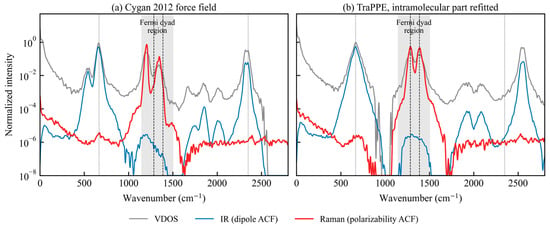
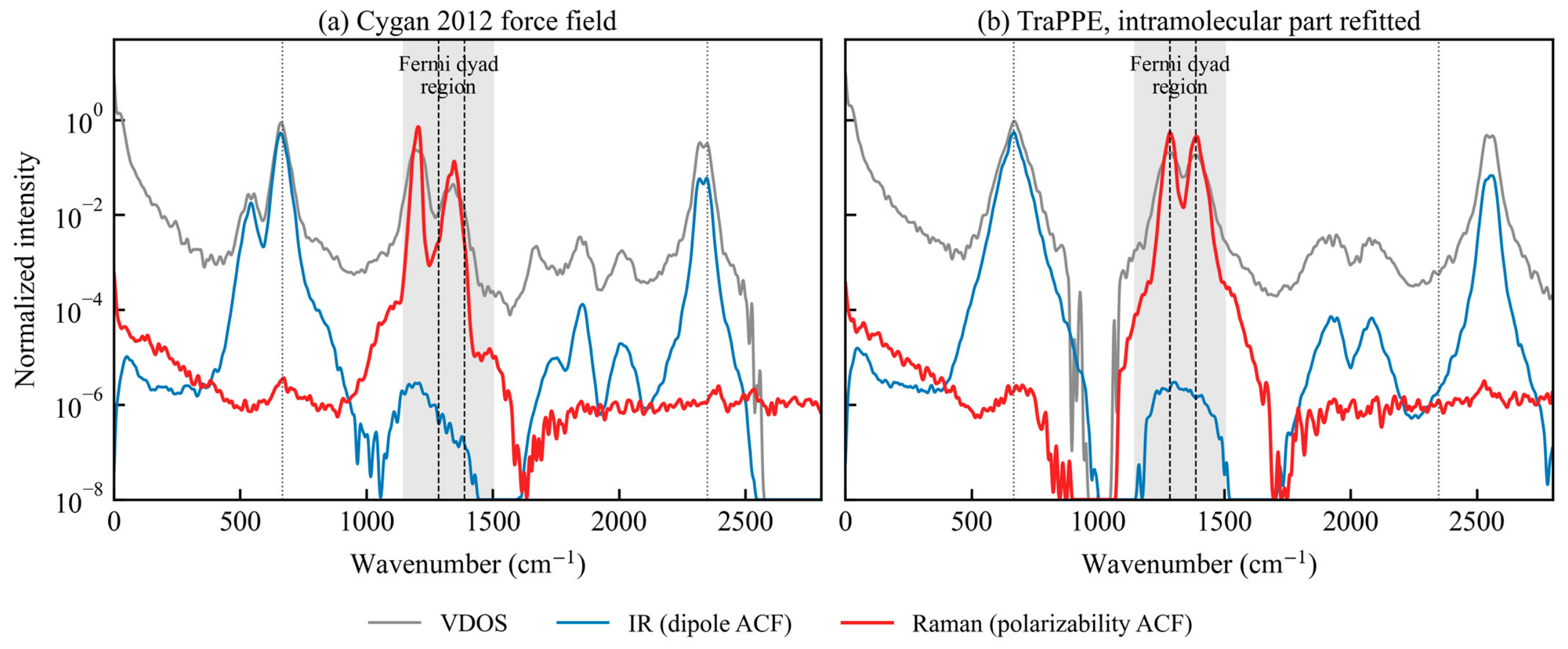
The CO₂ molecule is centrosymmetric, and in a model with fixed point charges the mutual exclusion rule holds. The dipole moment M = Σq_ir_i does not change during the symmetric stretch, because the carbon remains stationary and the sum of the coordinates of the two oxygen atoms is constant. Hence ∂M/∂Q₁ ≡ 0 identically. Figure 1 shows the three channels computed from a single MD run for two force fields. The density of states is sensitive to all modes; the dipole channel correctly recovers ν₂ and ν₃. The polarizability channel gives the mirror image. It is dominated by the Fermi dyad, while ν₂ and ν₃ are suppressed by five to six orders of magnitude.

Figure 1. Three spectral channels from a single trajectory (310 K, ρ = 0.5149 g·cm⁻³; according to [33], this is 8.5 MPa). Shown are the vibrational density of states (VDOS), the infrared response from the dipole moment autocorrelation function, and the Raman response from the polarizability autocorrelation function, each normalized to its own maximum. (a) Force field of Cygan and co-workers [30]. (b) TraPPE with the rederived intramolecular part. Dashed lines mark the observed dyad; dotted lines mark ν₂ and ν₃. For clarity, the curves were median-filtered over five points (10 cm⁻¹) and lightly smoothed on the logarithmic scale.

2.2. Detuning and Coupling Constant

Table 1 lists the harmonic frequencies calculated analytically from the force field coefficients and the dyad obtained from trajectories at 298 K and ρ = 0.8189 g·cm⁻³. For each model the detuning δ = |ν₁−2ν₂| is given. For the rederived TraPPE model δ = 1.9 cm⁻¹, for the real molecule 1.8 cm⁻¹, and the dyad appears at 1285.4 and 1389.4 cm⁻¹ versus the observed 1285.4 and 1388.2 [34,35]. For the Cygan model δ = 95 cm⁻¹, for flexible EPM2 δ = 823 cm⁻¹, and both give a single band with no dyad. The coupling constant found from the splitting and the detuning via W = ½√(Δν²−δ²) equals 52.0 cm⁻¹; the spectroscopic value is 51.4 cm⁻¹. This coupling arises by itself when the equations of motion are integrated in Cartesian coordinates, where the reduced mass of the bending vibration depends on the instantaneous bond length. In normal coordinates this is exactly the Q₁Q₂² term [36], and classical dynamics reproduces its magnitude to within 1%.

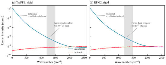
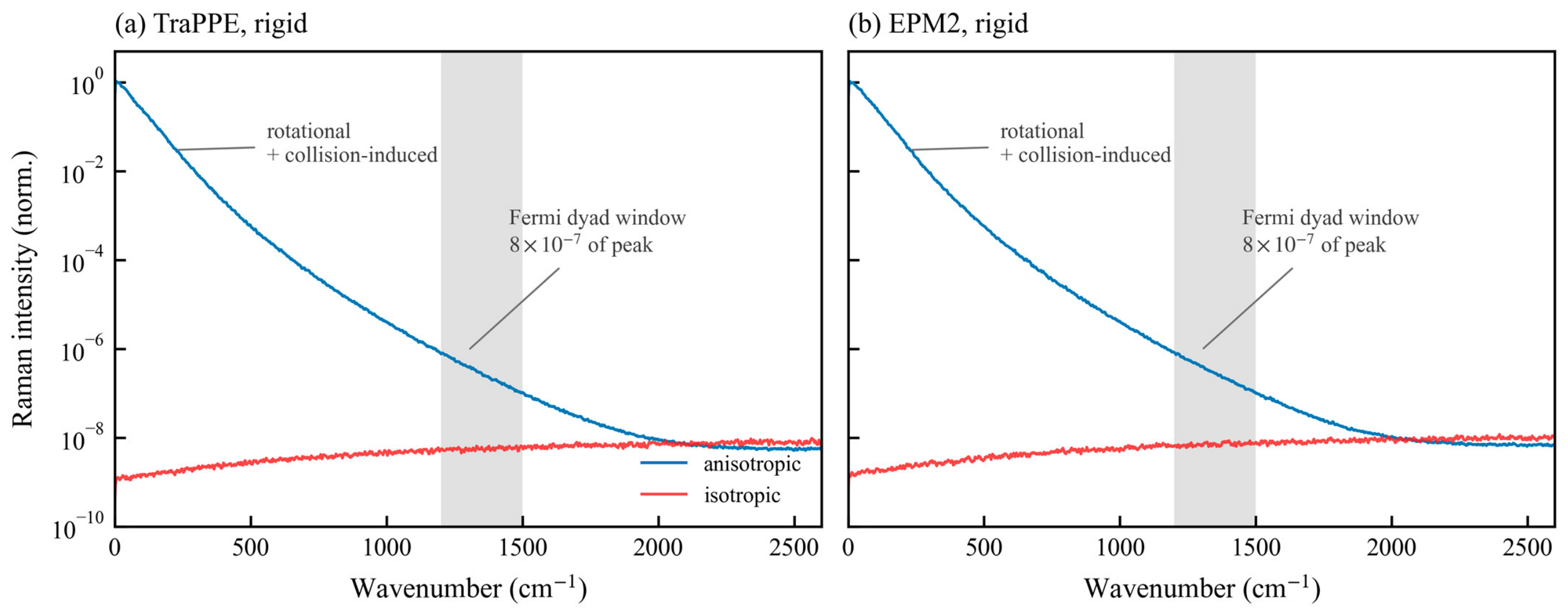
In rigid models the bond lengths are fixed, and the isotropic polarizability is constant to a relative accuracy of 3 × 10⁻⁶. Their isotropic channel reduces to numerical noise; the entire response is anisotropic and gathers into the rotational and collision-induced band below 400 cm⁻¹ (Figure 2). A molecule that cannot vibrate gives no dyad under any preparation and at any density, so the dyad of the flexible models has an intramolecular origin. In this state the rigid models reproduce the reference density to within −0.21% (TraPPE) and −1.23% (EPM2), so the absence of the dyad cannot be attributed to an incorrectly prepared state.

Figure 2. Raman response of the two rigid models at 298 K and 100 bar: (a) TraPPE; (b) EPM2. Shown are the isotropic (red) and anisotropic (blue) channels, each normalized to the maximum of the rotational band. The shaded strip marks the Fermi dyad window. With fixed bond lengths the isotropic channel is numerical noise. The anisotropic response is concentrated in the rotational and collision-induced band; in the dyad window it amounts to about 8 × 10⁻⁷ of its maximum.

Table 1. Harmonic frequencies from the force field coefficients, detuning δ = |ν₁−2ν₂|, Fermi dyad from trajectories at 298 K and ρ = 0.8189 g·cm⁻³ (T_vib in all runs 299–302 K), and the NPT density error relative to the reference equation of state [33] in three reference states (280 K/150 bar, 320 K/250 bar, and 350 K/80 bar). The flexible models were equilibrated with the Langevin thermostat and the Nosé–Hoover barostat, the rigid ones with the standard NPT integrator, for which there is no equipartition problem. The reference states are chosen where the isotherm is steep. At the point on the Widom line (310 K, 8.5 MPa), a 57% change in density shifts the model pressure by only 1%, and NPT measures nothing there.

Model	Ν1	Ν2	δ	ν1−	ν1+	Δν	W	Δρ (%), Three States
TraPPE, rederived intramol. part (this work) [26]	1332.8	667.4	1.9	1285.4	1389.4	103.9	52.0	+0.37/+0.15/−1.30
class2 + bond–bond [37]	1281.2	667.4	53.6	1281.2	1385.6	104.3	44.7	−0.47/−0.58/−3.07
Cygan et al., 2012 [30]	1219.5	657.3	95.1	1200.8	—	—	—	−0.41/−0.50/−3.06
EPM2, flexible [27]	1375.4	1099.3	823.2	1377.0	—	—	—	−0.95/−13.08/−3.65
ReaxFF C/H/O [38]	reactive	—	—	—	—	—	—	−65.3/−51.8/−23.1
TraPPE, rigid [26]	no internal modes	—	—	—	—	—	—	−0.38/−0.83/−3.15
EPM2, rigid [27]	no internal modes	—	—	—	—	—	—	−1.45/−2.01/−4.95
Experiment [35]	1333.0	667.4	1.8	1285.4	1388.2	102.8	51.4	source [33]

All values are in cm⁻¹ except the last column.

Table 1. Harmonic frequencies from the force field coefficients, detuning δ = |ν₁−2ν₂|, Fermi dyad from trajectories at 298 K and ρ = 0.8189 g·cm⁻³ (T_vib in all runs 299–302 K), and the NPT density error relative to the reference equation of state [33] in three reference states (280 K/150 bar, 320 K/250 bar, and 350 K/80 bar). The flexible models were equilibrated with the Langevin thermostat and the Nosé–Hoover barostat, the rigid ones with the standard NPT integrator, for which there is no equipartition problem. The reference states are chosen where the isotherm is steep. At the point on the Widom line (310 K, 8.5 MPa), a 57% change in density shifts the model pressure by only 1%, and NPT measures nothing there.

Model	Ν1	Ν2	δ	ν1−	ν1+	Δν	W	Δρ (%), Three States
TraPPE, rederived intramol. part (this work) [26]	1332.8	667.4	1.9	1285.4	1389.4	103.9	52.0	+0.37/+0.15/−1.30
class2 + bond–bond [37]	1281.2	667.4	53.6	1281.2	1385.6	104.3	44.7	−0.47/−0.58/−3.07
Cygan et al., 2012 [30]	1219.5	657.3	95.1	1200.8	—	—	—	−0.41/−0.50/−3.06
EPM2, flexible [27]	1375.4	1099.3	823.2	1377.0	—	—	—	−0.95/−13.08/−3.65
ReaxFF C/H/O [38]	reactive	—	—	—	—	—	—	−65.3/−51.8/−23.1
TraPPE, rigid [26]	no internal modes	—	—	—	—	—	—	−0.38/−0.83/−3.15
EPM2, rigid [27]	no internal modes	—	—	—	—	—	—	−1.45/−2.01/−4.95
Experiment [35]	1333.0	667.4	1.8	1285.4	1388.2	102.8	51.4	source [33]

All values are in cm⁻¹ except the last column.

2.3. Thermostat and Vibrational Temperature

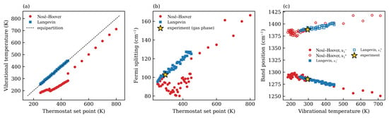
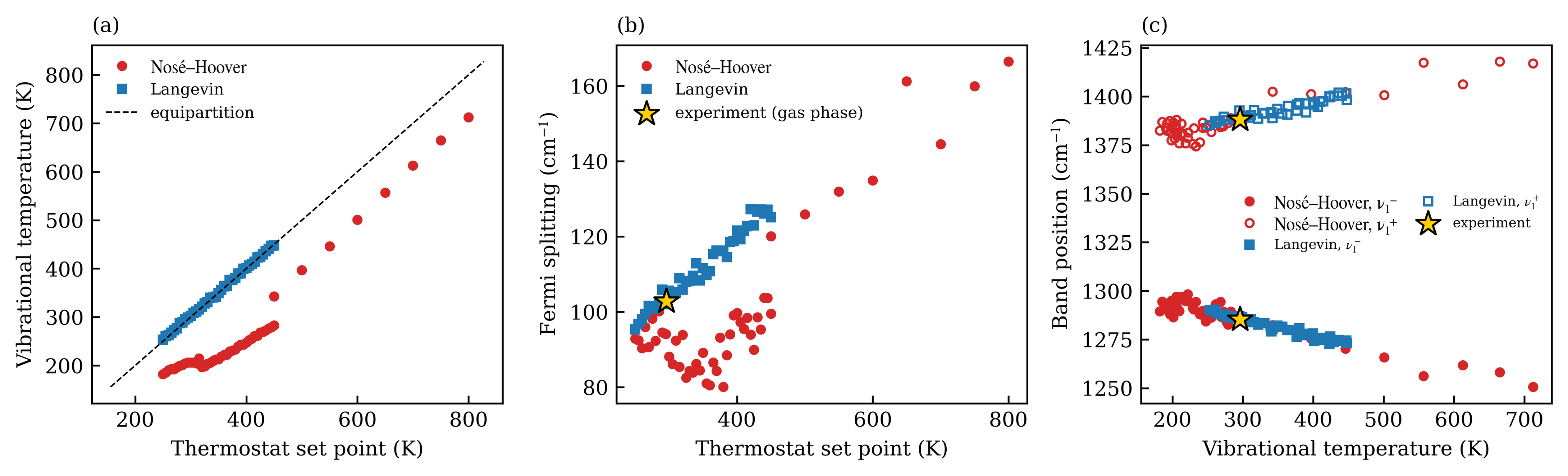
The global Nosé–Hoover thermostat [39,40] controls the total kinetic temperature through a single variable and assumes that the system will distribute the energy among the modes by itself. In CO₂ this assumption fails. The fundamental frequencies lie in the 667–2350 cm⁻¹ range, far above the collision frequencies, and vibrational–translational exchange is slow. Indeed, it is so slow that even the kinetics of the real gas is described by separate vibrational temperatures [41,42]. From four 1 ns runs, the relaxation time is ~390 ps at 310 K and ~180 ps at 450 K. Even after one nanosecond the vibrational temperature is 267.8 K at a target of 310 K and 419.3 K at a target of 450 K. The per-atom Langevin thermostat acts on every Cartesian degree of freedom, its projection onto any vibrational mode is nonzero, and the modes are filled directly. In the same runs it gives 312.4 K at a target of 310 K and 453.0 K at a target of 450 K, starting from the first sample. In NPT, the deficit of vibrational energy is compensated by overheated translational degrees of freedom. Their pressure is higher, the barostat responds by expanding the cell, and the density comes out underestimated. With the same force fields, changing only the thermostat reduces the density error of the flexible models from −66%, −50%, and −34% in the three reference states to +0.4%, +0.2%, and −1.3%. The spectra change strongly as well. For instance, our own earlier simulation [22] along an isobar ran at T_vib = 182–283 K, although the target temperatures were 250–450 K, and the splitting therefore shifted by about twenty wavenumbers. To demonstrate this effect, Figure 3 compares two series of simulations with the same model, the same code, and the same density, differing only in the thermostat (Figure 3a). In target-temperature coordinates the series diverge (Figure 3b), whereas in vibrational temperature coordinates they fall on a single curve (Figure 3c). The damping time determines how rapidly the Langevin thermostat removes the vibrational temperature deficit. Since no Langevin friction is applied during NVE production, it cannot directly broaden the calculated bands. A parametric study of equilibration times was outside the scope of this work. The spectral comparison relies instead on the direct check that the target T_vib was reached before production.

Figure 3. Simulations with the same model, code, and density at different thermostats. (a) Vibrational temperature versus the target temperature. (b) Dyad splitting versus the target temperature; the star marks the experimental point. (c) Component positions versus the vibrational temperature.

2.4. Response of the Dyad to Vibrational Temperature and Density

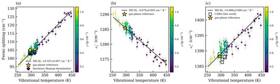
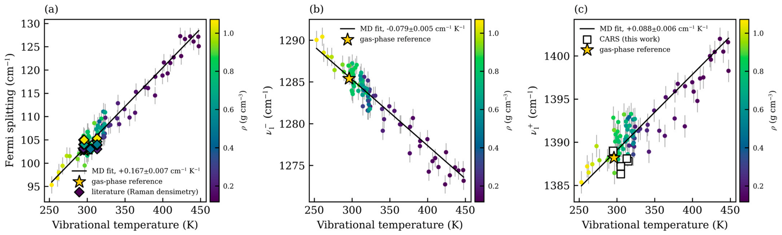
Figure 4 collects the results for 86 states (three isotherms at 298, 311, and 320 K with thirteen pressures each, plus a run along an isobar); density is encoded by color. A joint regression over T_vib and ρ gives ∂(Δν)/∂T_vib = +0.167 ± 0.007 cm⁻¹ K⁻¹ and ∂(Δν)/∂ρ = +1.8 ± 1.0 cm⁻¹/(g·cm⁻³). The dyad components shift in opposite directions, the lower one with a slope of −0.079 ± 0.005 cm⁻¹ K⁻¹ and the upper one with +0.088 ± 0.006 cm⁻¹ K⁻¹. Anharmonicity shifts the overtone 2ν₂ more strongly than the fundamental ν₁ as T_vib grows, and the detuning δ becomes a function of vibrational temperature. The component positions are given by the two-level resonance model E± = (E₁ + E₂)/2 ± ½√(δ² + 4W²), where E₁ and E₂ denote the unperturbed ν₁ and 2ν₂ levels. The first term sets the center of the pair, the second half the splitting. From the measured slopes, the pair center shifts by only +0.005 cm⁻¹ K⁻¹, while the half-splitting grows with |δ| by 0.083 cm⁻¹ K⁻¹. The upper component therefore moves up and the lower one down, and their slopes are almost equal in magnitude. With growing |δ|, the ν₁ and 2ν₂ states also mix more weakly. This is the response of the classical MD model, and for real CO₂ it is anomalously large. Heating CO₂ at constant density gives ∂Δ/∂T = +0.0011 ± 0.0042 cm⁻¹ K⁻¹ [17]; that is, over the 20–200 °C interval the slope is zero within the uncertainty. The computed slope of 0.167 cm⁻¹ K⁻¹ over our 250–450 K range would shift the splitting by 33 cm⁻¹, roughly 13 times the entire 2.5 cm⁻¹ interval that the splitting traverses from rarefied gas to liquid-like density. Such a shift could not go unnoticed in the experiment.

Figure 4. Splitting and component positions versus vibrational temperature for 86 states (three isotherms and one isobar); density is encoded by color. Slopes +0.167, −0.079, and +0.088 cm⁻¹ K⁻¹. Points differing in density by a factor of nine lie on the same straight line. The diamonds in (a) show equilibrium Raman data—direct measurements and published densimeter calibrations—reduced to the calibration temperatures [12,14,15,16,17,43]. At equilibrium the vibrational temperature equals the thermodynamic temperature. Panels (a–c) show the dyad splitting, lower-component position, and upper-component position, respectively.

The apparent contradiction is explained by the population of vibrational levels. The fraction of molecules on a level with energy hcν is proportional to g × exp(−hcν/k_BT), where g denotes the degeneracy and hc/k_B = 1.4388 cm·K. At 298 K for ν₁ = 1333 cm⁻¹ the exponent equals 1.4388×1333/298 = 6.44, and the first excited ν₁; level is populated at 1.6 × 10⁻³, i.e., about 0.16% of the molecules. For the bending vibration (ν₂ = 667.4 cm⁻¹) the Boltzmann factor is exp(−3.22) = 0.040, and, accounting for the twofold degeneracy, about 7.4% of the molecules carry one bending quantum. For ν₃ = 2349 cm⁻¹ the factor is 1.2 × 10⁻⁵. The vibrational partition function Z = (1−x₁)⁻¹(1−x₂)⁻²(1−x₃)⁻¹, where xᵢ = exp(−hcνᵢ/k_BT), equals 1.087, so 1/Z ≈ 92% of the molecules are in the ground vibrational state. The vibrational temperature of a real ensemble therefore can hardly change. In a classical simulation the vibrations are populated continuously, and T_vib becomes a genuine control variable on which the spectrum depends. Within this interpretation one can attempt to recover the “true” spectrum (see Section 2.5). If a stationary MD trajectory is split into 8 ps windows and the dyad is fitted in each window separately, the splitting varies from window to window by 5.3 cm⁻¹. At a slope of 0.167 cm⁻¹ K⁻¹ this gives the vibrational temperature of a single window to within about ±32 K. This is enough to distinguish an equilibrated cell from one in which the vibrational subsystem has not yet reached the target temperature and continues to draw energy from the translational degrees of freedom. The same slope shows the cost of a state preparation error. “Underheating” the vibrational subsystem by 100 K underestimates the splitting by 17 cm⁻¹, an order of magnitude above the intrinsic noise of the splitting estimate, and this error carries over entirely into any comparison with the experiment. Including or excluding ν₃ does not change T_vib under equipartition, provided that the mode count in the denominator is adjusted accordingly, because each classical vibrational mode has the same mean energy. Away from equilibrium, a definition excluding ν₃ gives a different value if the stretching modes are not equilibrated. The bond energy used here does not separate ν₁ and ν₃, so a numerical mode-resolved sensitivity test was not performed. Rotational/vibrational coupling also prevents a unique decomposition of the full Hamiltonian into vibrational and rotational parts. Accordingly, T_vib is the operational potential-energy temperature defined in Section 3.1, not a rigorous canonical temperature of an isolated vibrational subsystem. At full canonical equilibrium it coincides with the thermodynamic temperature.

The density coefficient can be compared with the experiment directly, and it agrees with it within the uncertainty. In this work it equals +1.8 ± 1.0 cm⁻¹/(g·cm⁻³); the published densimeter calibrations give 2.2–3.2 cm⁻¹/(g·cm⁻³) [12,13,14,15,16,17], and a least-squares fit to the literature gives 2.2 cm⁻¹/(g·cm⁻³), as shown in Figure 4. In a real experiment the Raman spectrum responds primarily to density. Moving along the 100 bar isobar from 313 to 320 K, the density drops from 0.629 to 0.448 g·cm⁻³ [33], and at the 2.2 cm⁻¹/(g·cm⁻³) calibration the splitting shifts by 0.40 cm⁻¹. The direct temperature response [17] over the same 7 K does not exceed 0.01 cm⁻¹, so about 98% of the shift comes from the density change.

2.5. Bandwidths and Inhomogeneous Broadening

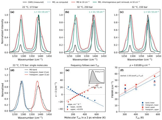
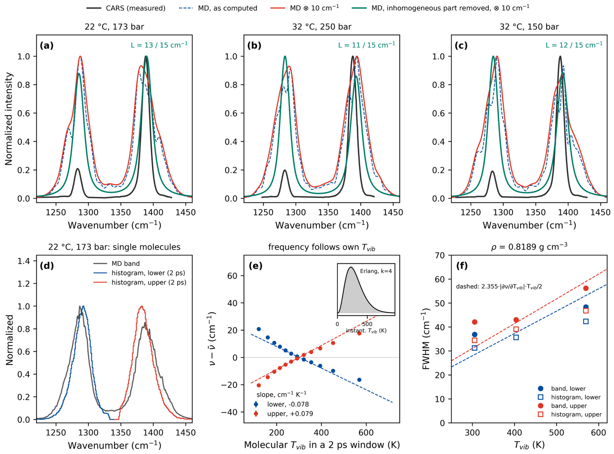
Figure 5a–c compare computed and measured spectra in three of the five states, before and after convolution with the 10 cm⁻¹ instrument function. Across all five states the computed upper component falls within 1386 to 1393 cm⁻¹ (experiment: 1386 to 1389 cm⁻¹) and the lower one within 1284 to 1287 cm⁻¹ (experiment: about 1284 cm⁻¹). The peak positions agree within the experimental error, while the linewidths differ strongly. The computed bands are 30 to 36 cm⁻¹ wide, the measured ones 13 cm⁻¹, and about 8 cm⁻¹ after accounting for the instrument function. The instrumental contribution is substantial for the measured widths. For Gaussian profiles, a measured FWHM of 13 cm⁻¹ and an instrumental FWHM of 10 cm⁻¹ correspond to an intrinsic width of (13²−10²)^1/2 = 8.3 cm⁻¹. Thus, the raw measured width is not used as the intrinsic linewidth. For the two states not shown in Figure 5, the computed positions and widths fall within the same ranges, and the comparison leads to the same conclusion. This overestimation of the widths is a manifestation of the classical limit of MD. In MD, the vibrational energy of a molecule is a continuous random variable, and for four vibrational modes it follows an Erlang distribution with a mean of 4kT and standard deviation of 2kT. Each molecule carries its own effective vibrational temperature with a spread σ_T ≈ T/2, about 149 K at room temperature. The band position depends on vibrational temperature with the measured slopes, so the ensemble is inhomogeneously broadened by 2.355 × (∂ν/∂T_vib) × σ_T. Without a single free parameter this gives 28 cm⁻¹ for the lower and 31 cm⁻¹ for the upper component, close to the computed widths. No such spread exists in the real system. As shown in Section 2.4, at 298 K about 92% of the molecules are in the ground vibrational state, and the observed width is homogeneous, set by dephasing and the rotational envelope.

Figure 5. (a–c) Computed and measured spectra in three states of dense CO₂: (a) compressed liquid, 22 °C, 173 bar; (b) supercritical fluid, 32 °C, 250 bar; (c) supercritical fluid, 32 °C, 150 bar. The black curve shows the CARS measurement, the blue dashed line the raw computation, the red curve the computation after convolution with the 10 cm⁻¹ instrument function, and the green curve the computation after removal of the inhomogeneous (Gaussian) contribution and convolution with the same function. L denotes the recovered homogeneous width of the lower and upper components. Each curve is normalized to its maximum. (d–f) Single-molecule check. (d) Computed band (gray curve, average of the spectra of 1000 molecules at 22 °C and 173 bar) and histograms of the instantaneous frequencies of molecules in 2 ps windows, blue for the lower and red for the upper component. About 4% of windows, where the maximum fell on the boundary of the search interval, were excluded. (e) Frequency shift of a molecule versus its own vibrational temperature in the same window. Dashed straight lines correspond to the ensemble regression slopes of Figure 4; the inset shows the distribution of the instantaneous vibrational temperature of a molecule and the Erlang distribution (k = 4). (f) Widths of the band and of the histogram along the 0.8189 g·cm⁻³ isochore versus vibrational temperature; dashed lines show the estimate 2.355 × |∂ν/∂T_vib| × T_vib/2.

We checked this explanation in two independent ways. First, each computed component was fitted with a Voigt profile whose Gaussian part describes the spread of molecular vibrational temperatures and whose Lorentzian part describes the homogeneous width. If the Gaussian width G is left free, the fit in all five states chooses G = 30 to 42 cm⁻¹, no less than the 28 to 33 cm⁻¹ estimate. With G fixed at this estimate, the homogeneous width L is 11 to 13 cm⁻¹ for the lower and 12 to 16 cm⁻¹ for the upper component (the L values are given in Figure 5a–c). The recovered band after convolution with the instrument function is 17 to 21 cm⁻¹ wide versus the measured 10 to 14 cm⁻¹ (Figure 5a–c, green curves), and the component positions do not change. Removing the inhomogeneous contribution reduces the width discrepancy from a factor of three to four to about one and a half. The Voigt analysis assumes a linear relation between frequency and T_vib over the molecular distribution, an approximately Gaussian distribution of molecular frequencies, and a quasistatic Gaussian contribution on the timescale of homogeneous dephasing. The Lorentzian component is assumed to be common to all molecules, and the two contributions are combined by convolution. These assumptions are approximate because the bending/energy correlation decays within 1 to 3 ps and the frequency/temperature slope varies at high T_vib. The Voigt fit therefore estimates the inhomogeneous contribution rather than providing a unique decomposition of the line shape.

The second check required separate simulations storing the trajectories of 1000 molecules (50 ps, saved every 4 fs) at 22 °C and 173 bar and along the 0.8189 g·cm⁻³ isochore at 298, 400, and 550 K. In the bond polarizability model, the isotropic polarizability of a molecule is proportional to the sum of the bond lengths r₁ + r₂. A windowed Fourier transform of this quantity (2 ps Hann window, 1 ps step) gives the instantaneous frequencies of both components of an individual molecule, and the window-averaged potential vibrational energy gives its own vibrational temperature. The instantaneous vibrational temperature of a molecule is indeed gamma-distributed with shape parameter k = 4.1–4.2 and a standard deviation of 146 K at T_vib = 300 K (inset in Figure 5e), i.e., it follows the Erlang law. The frequency of each molecule tracks its own vibrational temperature with slopes of −0.078 and +0.079 cm⁻¹ K⁻¹ (Figure 5e), almost the same as the ensemble regression over 86 states, which gave (−0.079 and +0.088 cm⁻¹ K⁻¹). The histogram of instantaneous frequencies reproduces the computed band shape (Figure 5d); its width is 31 and 33 cm⁻¹ versus the band width of 31 and 37 cm⁻¹. As T_vib grows from 300 to 570 K, the widths of the band and of the histogram grow monotonically from 31–37 to 42–56 cm⁻¹ (Figure 5f), but more slowly than in proportion to T. The slope of frequency against the molecular vibrational temperature drops to 0.051 cm⁻¹ K⁻¹ at 570 K, and the linear law holds only approximately. Under such conditions the stretching-vibration energy of a molecule persists for a long time. Its autocorrelation function decays to 0.6 in 10 ps and to 0.3–0.4 in 40 ps, so this contribution is quasistatic and broadens the band inhomogeneously. The bending-vibration energy loses correlation within 1–3 ps, so its contribution is partially motionally averaged and adds to the homogeneous width. This is how we explain the residual homogeneous width, but what fraction of the residual 11–16 cm⁻¹ this mechanism provides was not checked quantitatively. Both contributions arise from the continuous classical distribution of vibrational energy and are absent in the vibrationally frozen real ensemble. Classical molecular dynamics therefore systematically over-broadens anharmonic vibrational bands while hardly shifting them.

2.6. Component Intensities

Classical molecular dynamics does not reproduce the intensity ratio within the dyad. In the CARS measurement the upper component is about 4.8 times stronger than the lower one, which at I ∝ |χ⁽³⁾|² corresponds to a ratio of about 2.2 in spontaneous Raman scattering; the computation gives only 1.05. The Raman intensity recovered from the trajectory is limited by the polarizability model [44,45], and the derivatives of polarizability with respect to the bond lengths in this model are taken as order-of-magnitude estimates and have never been calibrated. The 2ν₂ overtone gains intensity through the second derivative of polarizability with respect to the bending coordinate, and it is defined as the worst. Calibrating these derivatives against density functional calculations requires separate work.

3. Materials and Methods

3.1. Models and Simulation Protocol

In this work we compared seven CO₂ models (Table 2): rigid TraPPE [26] and EPM2 [27], flexible EPM2, the flexible model of Cygan and co-workers [30], the class2 model with a bond–bond interaction [37], the ReaxFF C/H/O reactive force field [38], and a TraPPE variant in which only the intramolecular part was rederived.

Table 2. Parameters of the CO₂ models. Listed are the Lennard-Jones parameters ε/k_B and σ for the C and O atoms, the carbon charge q_C (the oxygen charge q_O = −q_C/2), the equilibrium bond length r₀, and the bond and angle force constants k_r and k_θ in the convention E = ½k(x–x₀)². Cross parameters were obtained by the Lorentz–Berthelot rule; intramolecular Lennard-Jones and Coulomb interactions are excluded; equilibrium angle 180°.

Model	εC/kB, K	σC, Å	εO/kB, K	σO, Å	qC, e	r0, Å	kr, N/m	kθ, kcal/(Mol·Rad2)
TraPPE, rigid [26]	27.0	2.800	79.0	3.050	+0.700	1.160	—	—
EPM2, rigid [27]	28.13	2.757	80.51	3.033	+0.6512	1.149	—	—
EPM2, flexible [27]	28.13	2.757	80.51	3.033	+0.6512	1.149	1783.3	295.4
Cygan et al. [30]	28.14	2.800	80.38	3.028	+0.6512	1.162	1402.0	108.0
class2 + bond–bond [37] a	28.14	2.800	80.38	3.028	+0.6512	1.162	1547.3	111.3
ReaxFF C/H/O [38] b	—	—	—	—	—	—	—	—
TraPPE, rederived intramolecular part (this work)	27.0	2.800	79.0	3.050	+0.700	1.160	1674.8	110.96

^a An additional cross bond–bond constant k_rr’ = 127.5 N/m and third- and fourth-order terms in the bond potential. ^b Parameters are taken from the field file [38]; the charges are recomputed at each step by the electronegativity equalization method (QEq).

Table 2. Parameters of the CO₂ models. Listed are the Lennard-Jones parameters ε/k_B and σ for the C and O atoms, the carbon charge q_C (the oxygen charge q_O = −q_C/2), the equilibrium bond length r₀, and the bond and angle force constants k_r and k_θ in the convention E = ½k(x–x₀)². Cross parameters were obtained by the Lorentz–Berthelot rule; intramolecular Lennard-Jones and Coulomb interactions are excluded; equilibrium angle 180°.

Model	εC/kB, K	σC, Å	εO/kB, K	σO, Å	qC, e	r0, Å	kr, N/m	kθ, kcal/(Mol·Rad2)
TraPPE, rigid [26]	27.0	2.800	79.0	3.050	+0.700	1.160	—	—
EPM2, rigid [27]	28.13	2.757	80.51	3.033	+0.6512	1.149	—	—
EPM2, flexible [27]	28.13	2.757	80.51	3.033	+0.6512	1.149	1783.3	295.4
Cygan et al. [30]	28.14	2.800	80.38	3.028	+0.6512	1.162	1402.0	108.0
class2 + bond–bond [37] a	28.14	2.800	80.38	3.028	+0.6512	1.162	1547.3	111.3
ReaxFF C/H/O [38] b	—	—	—	—	—	—	—	—
TraPPE, rederived intramolecular part (this work)	27.0	2.800	79.0	3.050	+0.700	1.160	1674.8	110.96

^a An additional cross bond–bond constant k_rr’ = 127.5 N/m and third- and fourth-order terms in the bond potential. ^b Parameters are taken from the field file [38]; the charges are recomputed at each step by the electronegativity equalization method (QEq).

In this variant the Lennard-Jones parameters and charges of TraPPE were left unchanged, and the bond and angle force constants k_r and k_θ were found from the gas-phase fundamental frequencies of the isolated molecule ν₁ = 1333.0 cm⁻¹ and ν₂ = 667.4 cm⁻¹. In the harmonic approximation ν₁ = (2πc)⁻¹(k_r/m_O)^1/2 and ν₂ = (2πc)⁻¹[2k_θ(1/m_O + 2/m_C)]^1/2/r₀, from which at r₀ = 1.16 Å we obtain k_r = 1674.8 N/m and k_θ = 110.96 kcal·mol⁻¹·rad⁻². The near degeneracy ν₁ ≈ 2ν₂ follows directly from these two constants. The coupling constant W requires no separate parameter and arises from the kinematics of the molecule (Section 2.2). The model was not fitted to the dyad positions, the splitting, the bandwidths, or any condensed-phase properties. The gas-phase parameterization determines the harmonic intramolecular potential and contains no explicit temperature or density dependence. Its use in the dense fluid assumes that intermolecular interactions do not strongly perturb the local intramolecular potential. The Lennard-Jones parameters and charges remain those of TraPPE, so the condensed-phase interactions are unchanged. The present calculations test this approximation for the dyad up to 450 K and for NPT density at the three states listed in Table 2, where the density errors are +0.37%, +0.15%, and −1.30%. At higher temperatures, anharmonicity and rotational/vibrational coupling become increasingly important. The gas-phase frequencies therefore do not guarantee the same accuracy outside the investigated range.

The main simulations were performed in the microcanonical ensemble on 8000 molecules (24,000 atoms; 1000 molecules for ReaxFF) with the LAMMPS package (https://www.lammps.org/, accessed on 8 November 2026) [46]. The Raman response was obtained from the autocorrelation function of the system polarizability [47,48], which was recovered from the trajectory within the bond polarizability model [44,45]. The infrared response is given by the autocorrelation function of the dipole moment, the vibrational density of states by the autocorrelation function of velocities, and all three spectra are recovered from a single run. The main 50–100 ps cycle gives a resolution of 0.33–0.67 cm⁻¹, an order of magnitude better than the width of the narrowest band of interest. The spectra were averaged over eight independent groups of molecules and over Welch windows, and the dyad was fitted with two Lorentzians. Each state was simulated in several stages. First, the system was heated in the NVT ensemble on the initial lattice, and the cell was deformed to the target density taken from the reference equation of state [33]. Then followed an equilibration with the per-atom Langevin thermostat, a check of energy conservation in the NVE ensemble, and the final production run in the NVE ensemble. The thermostat parameters control the rate of equilibration. They do not enter the spectral calculation because the production trajectory is generated in NVE with the thermostat switched off. We did not perform a systematic sweep of the Nosé–Hoover relaxation time or the Langevin damping time. Instead, the vibrational temperature was checked before the production run to verify equilibration.

The vibrational temperature was monitored at all stages as T_vib = (E_bond + E_bend)/(2Nk_B), where N is the number of CO₂ molecules, k_B is Boltzmann’s constant, and E_bond and E_bend are the total potential energies of the bond and angle terms. The denominator accounts for four classical vibrational modes per molecule: the symmetric stretch ν₁, the asymmetric stretch ν₃, and the doubly degenerate bend ν₂. The bond terms contain ν₁ and ν₃, while the angle term represents the two bending components in Cartesian dynamics. For a harmonic system, the mean potential energy of each mode is k_BT/2, which gives the factor 2Nk_B for four modes. Thus, T_vib is an operational potential-energy temperature that includes all four vibrational modes.

3.2. CARS Measurements

CARS spectra of dense CO₂ were measured in five states at 22 to 42 °C and 100 to 250 bar, four of them supercritical and one in a compressed liquid (22 °C, 173 bar). The sample was held in a high-pressure cell; the measurements were performed on the custom-built two-pulse collinear broadband femtosecond CARS setup of the laser complex of the Shared Research Facilities of the Federal Research Center of Chemical Physics, Russian Academy of Sciences. The pump pulse (λ = 719 nm, τ ≈ 40 fs, from an optical parametric amplifier) was narrowed by a slit filter to FWHM ≤ 10 cm⁻¹, and this width sets the spectral resolution. The pump energy before the cell was about 50 nJ. The broadband Stokes pulse (λ ≈ 800 nm, τ ≈ 60 fs, ν ≈ 500 cm⁻¹) received a quadratic chirp from a spatial light modulator (SLM); its energy was about 300 nJ. The beams at a repetition rate of 1 kHz were focused into the cell by f = 50 mm lenses. The anti-Stokes signal was collected in the forward phase-matching direction, dispersed by a spectrograph with a 300 mm focal length, and recorded by a camera cooled to −50 °C with a 100 ms exposure. For linewidth analysis, the instrument function was approximated by a Gaussian FWHM of 10 cm⁻¹. Before any comparison of widths, the computed spectra were convolved with this instrument function.

3.3. Use of Generative AI

The generative model Qwen 3.8-27b, deployed on a local Nvidia DGX Spark server (NVIDIA Corporate, Santa Clara, CA, USA), was used for writing and debugging trajectory-processing scripts, statistical analysis, and editing the manuscript text, and translation to English. All results, code, and wording were verified by the authors, who bear full responsibility for them.

4. Conclusions

Classical molecular dynamics quantitatively reproduces the Fermi dyad of carbon dioxide through Fourier analysis of the polarizability autocorrelation function. The positions of the Raman-active lines are recovered to within 1–3 cm⁻¹, and the Fermi resonance constant to about 1%. For this, the vibrations must be truly equilibrated, which the global Nosé–Hoover thermostat does not ensure on practical timescales. The computed bands remain three to four times broader than the measured ones, and this is a property of classical modeling. From individual-molecule trajectories, the vibrational energy of each molecule follows an Erlang distribution, and the frequency of a molecule tracks its own vibrational temperature. The real ensemble at near-room temperatures is vibrationally frozen. Removing this inhomogeneous contribution reduces the width discrepancy to about a factor of one and a half.

References

- Crespi, F.; Gavagnin, G.; Sánchez, D.; Martínez, G.S. Supercritical carbon dioxide cycles for power generation: A review. Appl. Energy 2017, 195, 152–183. [Google Scholar] [CrossRef] [Scilit]
- Guo, J.-Q.; Li, M.-J.; He, Y.-L.; Jiang, T.; Ma, T.; Xu, J.-L.; Cao, F. A systematic review of supercritical carbon dioxide (S-CO2) power cycle for energy industries: Technologies, key issues, and potential prospects. Energy Convers. Manag. 2022, 258, 115437. [Google Scholar] [CrossRef] [Scilit]
- Reverchon, E.; De Marco, I. Supercritical fluid extraction and fractionation of natural matter. J. Supercrit. Fluids 2006, 38, 146–166. [Google Scholar] [CrossRef] [Scilit]
- Jessop, P.G.; Ikariya, T.; Noyori, R. Homogeneous Catalysis in Supercritical Fluids. Chem. Rev. 1999, 99, 475–494. [Google Scholar] [CrossRef] [Scilit] [PubMed]
- Reverchon, E.; Adami, R. Nanomaterials and supercritical fluids. J. Supercrit. Fluids 2006, 37, 1–22. [Google Scholar] [CrossRef] [Scilit]
- Simeoni, G.G.; Bryk, T.; Gorelli, F.A.; Krisch, M.; Ruocco, G.; Santoro, M.; Scopigno, T. The Widom line as the crossover between liquid-like and gas-like behaviour in supercritical fluids. Nat. Phys. 2010, 6, 503–507. [Google Scholar] [CrossRef] [Scilit]
- Asharchuk, N.M.; Yusupov, V.I.; Mareev, E.I. Role of clustering in the anomalous properties of supercritical fluids. Mater. Today 2025, 82, 49–56. [Google Scholar] [CrossRef] [Scilit]
- Fan, J.; Ly, N.; Ihme, M. Heterogeneous Cluster Energetics and Nonlinear Thermodynamic Response in Supercritical Fluids. Phys. Rev. Lett. 2024, 133, 248001. [Google Scholar] [CrossRef] [Scilit] [PubMed]
- Banuti, D.T.; Raju, M.; Ihme, M. Between supercritical liquids and gases—Reconciling dynamic and thermodynamic state transitions. J. Supercrit. Fluids 2020, 165, 104895. [Google Scholar] [CrossRef] [Scilit]
- Fomin, Y.D.; Ryzhov, V.N.; Tsiok, E.N.; Brazhkin, V.V. Thermodynamic properties of supercritical carbon dioxide: Widom and Frenkel lines. Phys. Rev. E 2015, 91, 022111. [Google Scholar] [CrossRef] [Scilit] [PubMed]
- Fermi, E. Über den Ramaneffekt des Kohlendioxyds. Z. Phys. 1931, 71, 250–259. [Google Scholar] [CrossRef] [Scilit]
- Garrabos, Y.; Tufeu, R.; Le Neindre, B.; Zalczer, G.; Beysens, D. Rayleigh and Raman scattering near the critical point of carbon dioxide. J. Chem. Phys. 1980, 72, 4637–4651. [Google Scholar] [CrossRef] [Scilit]
- Wright, R.B.; Wang, C.H. Density effect on the Fermi resonance in gaseous CO2 by Raman scattering. J. Chem. Phys. 1973, 58, 2893–2895. [Google Scholar] [CrossRef] [Scilit]
- Kawakami, Y.; Yamamoto, J.; Kagi, H. Micro-Raman densimeter for CO2 inclusions in mantle-derived minerals. Appl. Spectrosc. 2003, 57, 1333–1339. [Google Scholar] [CrossRef] [Scilit] [PubMed]
- Wang, X.; Chou, I.-M.; Hu, W.; Burruss, R.C.; Sun, Q.; Song, Y. Raman spectroscopic measurements of CO2 density: Experimental calibration with high-pressure optical cell (HPOC) and fused silica capillary capsule (FSCC) with application to fluid inclusion observations. Geochim. Cosmochim. Acta 2011, 75, 4080–4093. [Google Scholar] [CrossRef] [Scilit]
- Lamadrid, H.M.; Moore, L.R.; Moncada, D.; Rimstidt, J.D.; Burruss, R.C.; Bodnar, R.J. Reassessment of the Raman CO2 densimeter. Chem. Geol. 2017, 450, 210–222. [Google Scholar] [CrossRef] [Scilit]
- Hagiwara, Y.; Sogo, Y.; Takahata, K.; Yamamoto, J. Temperature dependence of CO2 densimetry using micro-Raman spectrometry at laboratory conditions. Geochem. J. 2018, 52, 379–383. [Google Scholar] [CrossRef] [Scilit]
- Cabaço, M.I.; Longelin, S.; Danten, Y.; Besnard, M. Transient dimer formation in supercritical carbon dioxide as seen from Raman scattering. J. Chem. Phys. 2008, 128, 074507. [Google Scholar] [CrossRef] [Scilit] [PubMed]
- Idrissi, A.; Ruckebusch, C.; Debus, B.; Boussekey, L.; Damay, P. Probing local structure of sub and supercritical CO2 by using two-dimensional Raman correlation spectroscopy. J. Mol. Liq. 2011, 164, 11–16. [Google Scholar] [CrossRef] [Scilit]
- Mareev, E.; Semenov, T.; Lazarev, A.; Minaev, N.; Sviridov, A.; Potemkin, F.; Gordienko, V. Optical diagnostics of supercritical CO2 and CO2–ethanol mixture in the Widom delta. Molecules 2020, 25, 5424. [Google Scholar] [CrossRef] [Scilit] [PubMed]
- Mazza, F.; Griffioen, N.; Castellanos, L.; Kliukin, D.; Bohlin, A. High-temperature rotational-vibrational O2–CO2 coherent Raman spectroscopy with ultrabroadband femtosecond laser excitation generated in-situ. Combust. Flame 2022, 237, 111738. [Google Scholar] [CrossRef] [Scilit]
- Asharchuk, N.M.; Mareev, E.I. Molecular Dynamics Simulation of the Raman Spectra of Supercritical Carbon Dioxide. Russ. J. Phys. Chem. B 2024, 18, 1729–1736. [Google Scholar] [CrossRef] [Scilit]
- Berens, P.H.; Wilson, K.R. Molecular dynamics and spectra. I. Diatomic rotation and vibration. J. Chem. Phys. 1981, 74, 4872–4882. [Google Scholar] [CrossRef] [Scilit]
- Thomas, M.; Brehm, M.; Fligg, R.; Vöhringer, P.; Kirchner, B. Computing vibrational spectra from ab initio molecular dynamics. Phys. Chem. Chem. Phys. 2013, 15, 6608–6626. [Google Scholar] [CrossRef] [Scilit] [PubMed]
- Jiang, H.; Economou, I.G.; Panagiotopoulos, A.Z. Molecular modeling of thermodynamic and transport properties for CO2 and aqueous brines. Acc. Chem. Res. 2017, 50, 751–758. [Google Scholar] [CrossRef] [Scilit] [PubMed]
- Potoff, J.J.; Siepmann, J.I. Vapor–liquid equilibria of mixtures containing alkanes, carbon dioxide, and nitrogen. AIChE J. 2001, 47, 1676–1682. [Google Scholar] [CrossRef] [Scilit]
- Harris, J.G.; Yung, K.H. Carbon Dioxide’s Liquid-Vapor Coexistence Curve And Critical Properties as Predicted by a Simple Molecular Model. J. Phys. Chem. 1995, 99, 12021–12024. [Google Scholar] [CrossRef] [Scilit]
- Persson, R.A.X. Gaussian charge polarizable interaction potential for carbon dioxide. J. Chem. Phys. 2011, 134, 034312. [Google Scholar] [CrossRef] [Scilit] [PubMed]
- Wang, F.-F.; Kumar, R.; Jordan, K.D. A distributed point polarizable force field for carbon dioxide. Theor. Chem. Acc. 2012, 131, 1132. [Google Scholar] [CrossRef] [Scilit]
- Cygan, R.T.; Romanov, V.N.; Myshakin, E.M. Molecular Simulation of Carbon Dioxide Capture by Montmorillonite Using an Accurate and Flexible Force Field. J. Phys. Chem. C 2012, 116, 13079–13091. [Google Scholar] [CrossRef] [Scilit]
- Saharay, M.; Balasubramanian, S. Ab initio molecular-dynamics study of supercritical carbon dioxide. J. Chem. Phys. 2004, 120, 9694–9702. [Google Scholar] [CrossRef] [Scilit] [PubMed]
- Glezakou, V.-A.; Rousseau, R.; Dang, L.X.; McGrail, B.P. Structure, dynamics and vibrational spectrum of supercritical CO2/H2O mixtures from ab initio molecular dynamics as a function of water cluster formation. Phys. Chem. Chem. Phys. 2010, 12, 8759–8771. [Google Scholar] [CrossRef] [Scilit] [PubMed]
- Span, R.; Wagner, W. A New Equation of State for Carbon Dioxide Covering the Fluid Region from the Triple-Point Temperature to 1100 K at Pressures up to 800 MPa. J. Phys. Chem. Ref. Data 1996, 25, 1509–1596. [Google Scholar] [CrossRef] [Scilit]
- Stoicheff, B.P. High resolution Raman spectroscopy of gases: XI. Spectra of CS2 and CO2. Can. J. Phys. 1958, 36, 218–230. [Google Scholar] [CrossRef] [Scilit]
- Howard-Lock, H.E.; Stoicheff, B.P. Raman intensity measurements of the Fermi diad ν1, 2ν2 in 12CO2 and 13CO2. J. Mol. Spectrosc. 1971, 37, 321–326. [Google Scholar] [CrossRef] [Scilit]
- Herzberg, G. Molecular Spectra and Molecular Structure. II. Infrared and Raman Spectra of Polyatomic Molecules; Van Nostrand: New York, NY, USA, 1945. [Google Scholar]
- Hwang, M.J.; Stockfisch, T.P.; Hagler, A.T. Derivation of Class II Force Fields. 2. Derivation and Characterization of a Class II Force Field, CFF93, for the Alkyl Functional Group and Alkane Molecules. J. Am. Chem. Soc. 1994, 116, 2515–2525. [Google Scholar] [CrossRef] [Scilit]
- Chenoweth, K.; van Duin, A.C.T.; Goddard, W.A. ReaxFF Reactive Force Field for Molecular Dynamics Simulations of Hydrocarbon Oxidation. J. Phys. Chem. A 2008, 112, 1040–1053. [Google Scholar] [CrossRef] [Scilit] [PubMed]
- Nosé, S. A unified formulation of the constant temperature molecular dynamics methods. J. Chem. Phys. 1984, 81, 511–519. [Google Scholar] [CrossRef] [Scilit]
- Hoover, W.G. Canonical dynamics: Equilibrium phase-space distributions. Phys. Rev. A 1985, 31, 1695–1697. [Google Scholar] [CrossRef] [Scilit] [PubMed]
- Treanor, C.E.; Rich, J.W.; Rehm, R.G. Vibrational Relaxation of Anharmonic Oscillators with Exchange-Dominated Collisions. J. Chem. Phys. 1968, 48, 1798–1807. [Google Scholar] [CrossRef] [Scilit]
- Kustova, E.; Mekhonoshina, M. Novel approach for evaluation of CO2 vibrational relaxation times. Chem. Phys. Lett. 2021, 764, 138288. [Google Scholar] [CrossRef] [Scilit]
- Windisch, C.F.; Glezakou, V.-A.; Martin, P.F.; McGrail, B.P.; Schaef, H.T. Raman spectrum of supercritical C18O2 and re-evaluation of the Fermi resonance. Phys. Chem. Chem. Phys. 2012, 14, 2560–2566. [Google Scholar] [CrossRef] [Scilit] [PubMed]
- Paul, A.; Rubenstein, M.; Ruffino, A.; Masiuk, S.; Spanier, J.E.; Grinberg, I. Accuracy and limitations of the bond polarizability model in modeling of Raman scattering from molecular dynamics simulations. J. Chem. Phys. 2024, 161, 064305. [Google Scholar] [CrossRef] [Scilit] [PubMed]
- Paul, A.; Samala, N.R.; Grinberg, I. Generalized bond polarizability model for more accurate atomistic modeling of Raman spectra. J. Chem. Phys. 2025, 162, 054711. [Google Scholar] [CrossRef] [Scilit] [PubMed]
- Plimpton, S. Fast Parallel Algorithms for Short-Range Molecular Dynamics. J. Comput. Phys. 1995, 117, 1–19. [Google Scholar] [CrossRef] [Scilit]
- Schneider, T.; Stoll, E. Molecular-dynamics study of a three-dimensional one-component model for distortive phase transitions. Phys. Rev. B 1978, 17, 1302–1322. [Google Scholar] [CrossRef] [Scilit]
- Hartmann, J.M.; Boulet, C. Molecular dynamics simulations for CO2 spectra. III. Permanent and collision-induced tensors contributions to light absorption and scattering. J. Chem. Phys. 2011, 134, 184312. [Google Scholar] [CrossRef] [Scilit] [PubMed]
Disclaimer/Publisher’s Note: The statements, opinions and data contained in all publications are solely those of the individual author(s) and contributor(s) and not of MDPI and/or the editor(s). MDPI and/or the editor(s) disclaim responsibility for any injury to people or property resulting from any ideas, methods, instructions or products referred to in the content. |
© 2026 by the authors. Licensee MDPI, Basel, Switzerland. This article is an open access article distributed under the terms and conditions of the Creative Commons Attribution (CC BY) license.